RF simulations with COMSOL - ICPS · PDF file• Any structure that guides electromagnetic...
33
© Copyright 2017 COMSOL. Any of the images, text, and equations here may be copied and modified for your own internal use. All trademarks are the property of their respective owners. See www.comsol.com/trademarks. RF simulations with COMSOL ICPS 2017 Politecnico di Torino Aug. 10 th , 2017 Gabriele Rosati [email protected] 030 37.93.800
Transcript of RF simulations with COMSOL - ICPS · PDF file• Any structure that guides electromagnetic...
© Copyright 2017 COMSOL. Any of the images, text, and equations here may be copied and modified for your own internal use. All trademarks are the property of their respective owners. See www.comsol.com/trademarks.
RF simulations with COMSOL ICPS 2017
Politecnico di Torino
Aug. 10th, 2017 Gabriele Rosati
[email protected] 030 37.93.800
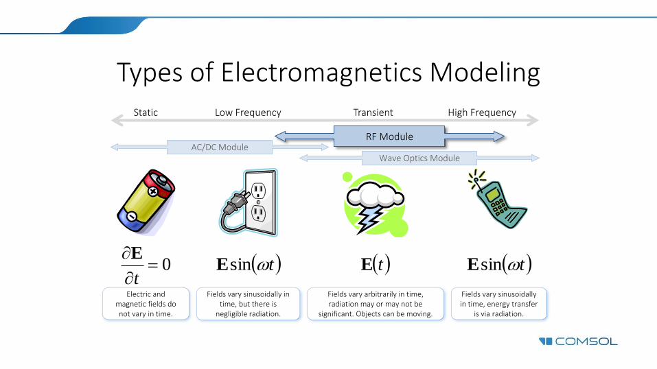
Types of Electromagnetics Modeling Static Low Frequency Transient High Frequency
0
t
E tsinE tE tsinE
Electric and magnetic fields do not vary in time.
Fields vary sinusoidally in time, energy transfer
is via radiation.
Fields vary arbitrarily in time, radiation may or may not be
significant. Objects can be moving.
Fields vary sinusoidally in time, but there is
negligible radiation.
AC/DC Module RF Module
Wave Optics Module
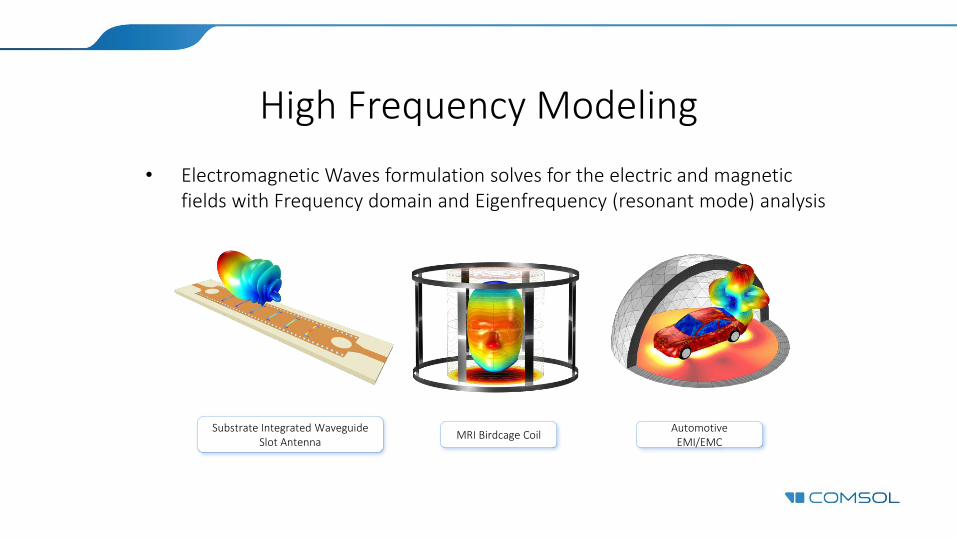
High Frequency Modeling
• Electromagnetic Waves formulation solves for the electric and magnetic fields with Frequency domain and Eigenfrequency (resonant mode) analysis
Substrate Integrated Waveguide Slot Antenna
Automotive EMI/EMC
MRI Birdcage Coil
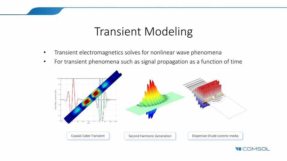
Transient Modeling
• Transient electromagnetics solves for nonlinear wave phenomena
• For transient phenomena such as signal propagation as a function of time
Second Harmonic Generation Coaxial Cable Transient Dispersive Drude-Lorentz media

Additional Formulations: Transmission Line Equations
• The Transmission Line Equation formulation solves for the electric potential along transmission lines
• For fast prototyping of transmission line circuits
0.5dB Equal-ripple Low Pass Filter
rr
r
BHB
MHB
HB
0
00
0
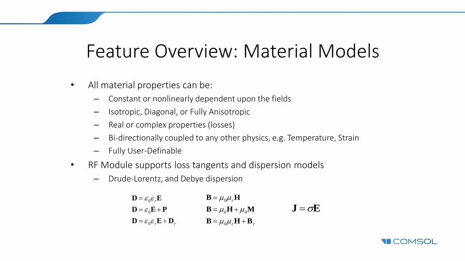
Feature Overview: Material Models
• All material properties can be:
– Constant or nonlinearly dependent upon the fields
– Isotropic, Diagonal, or Fully Anisotropic
– Real or complex properties (losses)
– Bi-directionally coupled to any other physics, e.g. Temperature, Strain
– Fully User-Definable
• RF Module supports loss tangents and dispersion models
– Drude-Lorentz, and Debye dispersion
rr
r
DED
PED
ED
0
0
0
EJ

rr
r
BHB
MHB
HB
0
00
0
Feature Overview: Material Models
• All material properties can be:
– Constant or nonlinearly dependent upon the fields
– Isotropic, Diagonal, or Fully Anisotropic
– Real or complex properties (losses)
– Bi-directionally coupled to any other physics, e.g. Temperature, Strain
– Fully User-Definable
• RF Module supports loss tangents and dispersion models
– Drude-Lorentz, and Debye dispersion
rr
r
DED
PED
ED
0
0
0
EJ
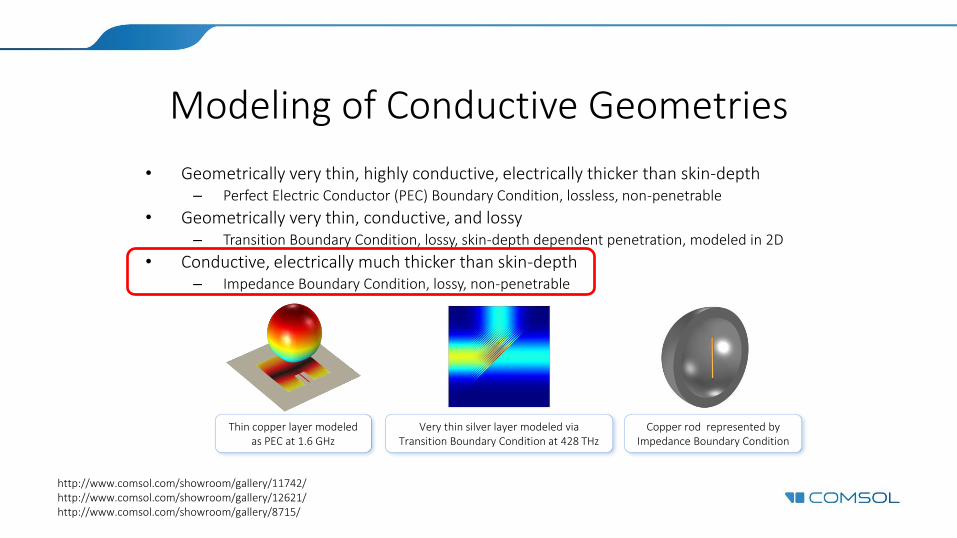
Modeling of Conductive Geometries
• Geometrically very thin, highly conductive, electrically thicker than skin-depth – Perfect Electric Conductor (PEC) Boundary Condition, lossless, non-penetrable
• Geometrically very thin, conductive, and lossy – Transition Boundary Condition, lossy, skin-depth dependent penetration, modeled in 2D
• Conductive, electrically much thicker than skin-depth – Impedance Boundary Condition, lossy, non-penetrable
http://www.comsol.com/showroom/gallery/11742/ http://www.comsol.com/showroom/gallery/12621/ http://www.comsol.com/showroom/gallery/8715/
Thin copper layer modeled as PEC at 1.6 GHz
Very thin silver layer modeled via Transition Boundary Condition at 428 THz
Copper rod represented by Impedance Boundary Condition
Feature Overview: Boundary Conditions
• Voltage source, Current source, & Insulating surfaces
• Thick volumes of electrically resistive, or conductive, material
• Thin layers of electrically resistive, or conductive, material
• Perfectly conducting boundaries
• Periodicity conditions
• Connections to external circuit models
• Lumped, Coaxial, and other Waveguide feeds
• Electromagnetic wave excitations
• Absorbing (Radiating) boundaries
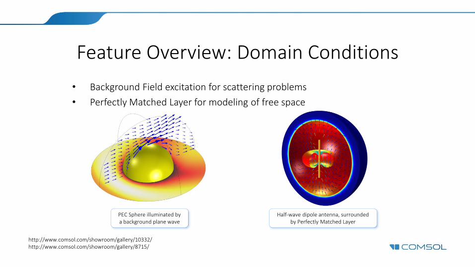
Feature Overview: Domain Conditions
• Background Field excitation for scattering problems
• Perfectly Matched Layer for modeling of free space
http://www.comsol.com/showroom/gallery/10332/ http://www.comsol.com/showroom/gallery/8715/
PEC Sphere illuminated by a background plane wave
Half-wave dipole antenna, surrounded by Perfectly Matched Layer

Feature Overview: Data Extraction
• Impedance, Admittance, and S-parameters
• Smith plot
• Touchstone file export
• Far-field plots for radiation
2221
1211
SS
SS
Lumped Parameters
Touchstone File Export Far-Field Radiation Pattern Smith Plot

• Any structure that guides electromagnetic waves along its structure can be considered a waveguide
• COMSOL can compute propagation constants, impedance, S-parameters
• COMSOL also solves the time-harmonic transmission line equation for the electric potential for electromagnetic wave propagation along one-dimensional transmission lines.
Typical examples Coaxial cable
Optical fibers and waveguides
Waveguides and Transmission Lines
z
rr
j
yx
jk
z)exp( ,
0
2
0
1
EE
0EE
01
VCiG
x
V
LiRx
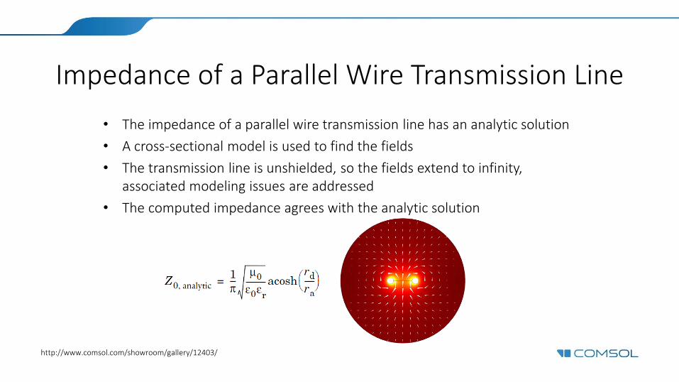
Impedance of a Parallel Wire Transmission Line
http://www.comsol.com/showroom/gallery/12403/
• The impedance of a parallel wire transmission line has an analytic solution
• A cross-sectional model is used to find the fields
• The transmission line is unshielded, so the fields extend to infinity, associated modeling issues are addressed
• The computed impedance agrees with the analytic solution

H-bend Waveguide 2D & 3D Model
• The transmission of a TE10 wave through a 90 ° bend in a waveguide is modeled
http://www.comsol.com/showroom/gallery/1421/

• Passive devices like couplers, power dividers, and filters can be realized by combining resonant structures and transmission lines. COMSOL calculates the fields distribution, impedance, and S-parameters
Typical examples 3dB Couplers and Power Dividers
Band-pass Filters
Passive Devices Example Models
nnn
n
rr
SS
SS
SSS
S
jk
...
:::::
...
..
1
2221
11211
0
2
0
10EE
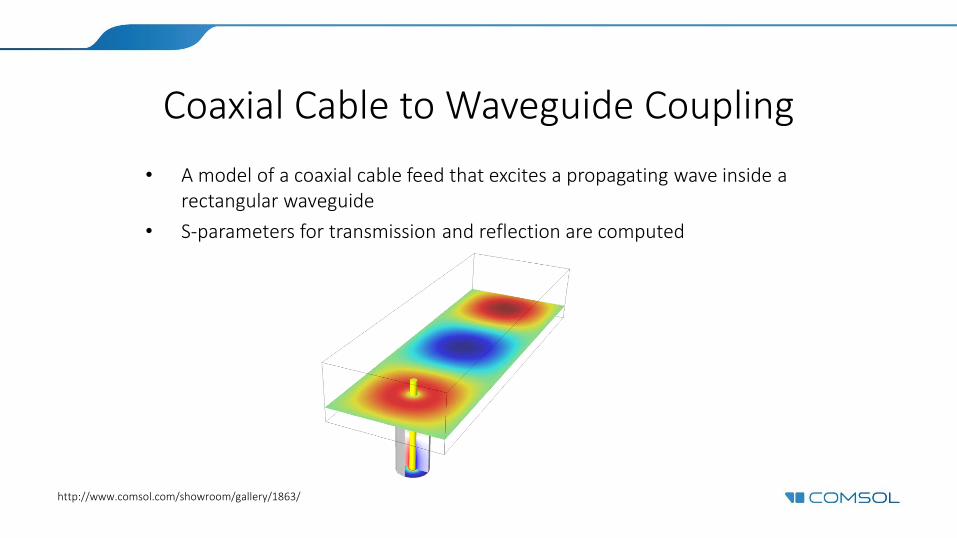
Coaxial Cable to Waveguide Coupling
• A model of a coaxial cable feed that excites a propagating wave inside a rectangular waveguide
• S-parameters for transmission and reflection are computed
http://www.comsol.com/showroom/gallery/1863/

Wilkinson Power Divider
• A Wilkinson power divider is a three-port lossless device and outperforms a T-junction divider and a resistive divider
• Computed S-parameters show good input matching and -3 dB evenly split output
• 100 Ohm resistor modeled via lumped element feature
http://www.comsol.com/showroom/gallery/12303/

Coplanar Waveguide (CPW) Bandpass Filter
• Excite and terminate two slots equally using multi-element uniform lumped ports
• Combination of interdigital capacitors (IDCs) and short-circuited stub inductors (SSIs)
http://www.comsol.com/showroom/gallery/12099/
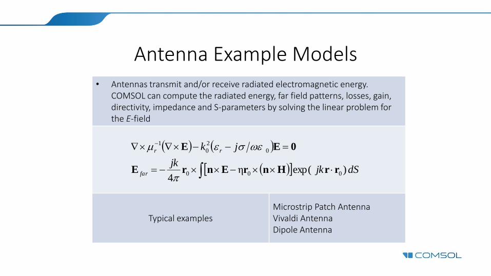
• Antennas transmit and/or receive radiated electromagnetic energy. COMSOL can compute the radiated energy, far field patterns, losses, gain, directivity, impedance and S-parameters by solving the linear problem for the E-field
Typical examples Microstrip Patch Antenna Vivaldi Antenna Dipole Antenna
Antenna Example Models
dSjkjk
jk
far
rr
)exp(η4
000
0
2
0
1
rrHnrEnrE
0EE

Corrugated Circular Horn Antenna
• Designed using a 2D axisymmetric model
• Low cross-polarization at the antenna aperture by combining TE mode excited at the circular waveguide feed and TM mode generated from the corrugated inner surface
http://www.comsol.com/showroom/gallery/15677/

Corrugated Circular Horn Antenna Simulator
• Enhance cross polarization ratio at the antenna aperture
• Various result analyses, simulation report, and documentation
• Very fast 2D axisymmetric simulation
• Customized intuitive GUI
http://www.comsol.com/showroom/gallery/22101/

4 x 2 Microstrip Patch Antenna Array
• Slot-coupled 4x2 array of patch antennas
• Controlling the phase and magnitude assigned to each element can steer the beam
• Far-Field radiation pattern is computed
http://www.comsol.com/showroom/gallery/12021/
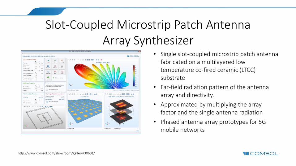
Slot-Coupled Microstrip Patch Antenna Array Synthesizer
• Single slot-coupled microstrip patch antenna fabricated on a multilayered low temperature co-fired ceramic (LTCC) substrate
• Far-field radiation pattern of the antenna array and directivity.
• Approximated by multiplying the array factor and the single antenna radiation
• Phased antenna array prototypes for 5G mobile networks
http://www.comsol.com/showroom/gallery/30601/
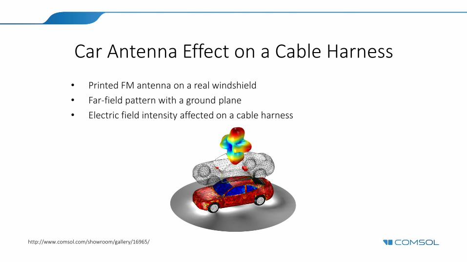
Car Antenna Effect on a Cable Harness
• Printed FM antenna on a real windshield
• Far-field pattern with a ground plane
• Electric field intensity affected on a cable harness
http://www.comsol.com/showroom/gallery/16965/

• Any structure that repeats in one, two, or all three dimensions can be treated as periodic, which allows for the analysis of a single unit cell, with Floquet Periodic boundary conditions
Typical examples Optical Gratings
Frequency Selective Surfaces Electromagnetic Band Gap Structures
Examples of Periodic Problems
))(exp( sdFsd j rrkEE
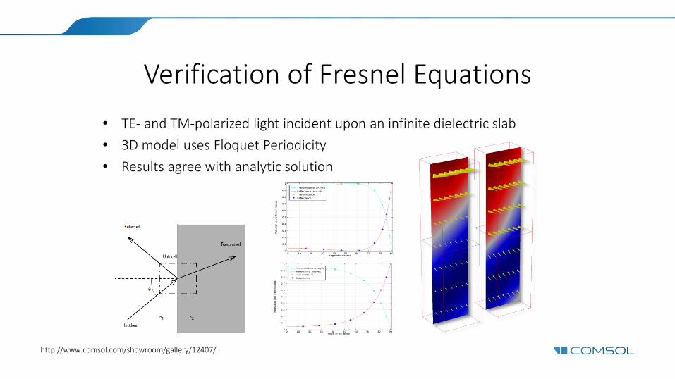
Verification of Fresnel Equations
http://www.comsol.com/showroom/gallery/12407/
• TE- and TM-polarized light incident upon an infinite dielectric slab
• 3D model uses Floquet Periodicity
• Results agree with analytic solution
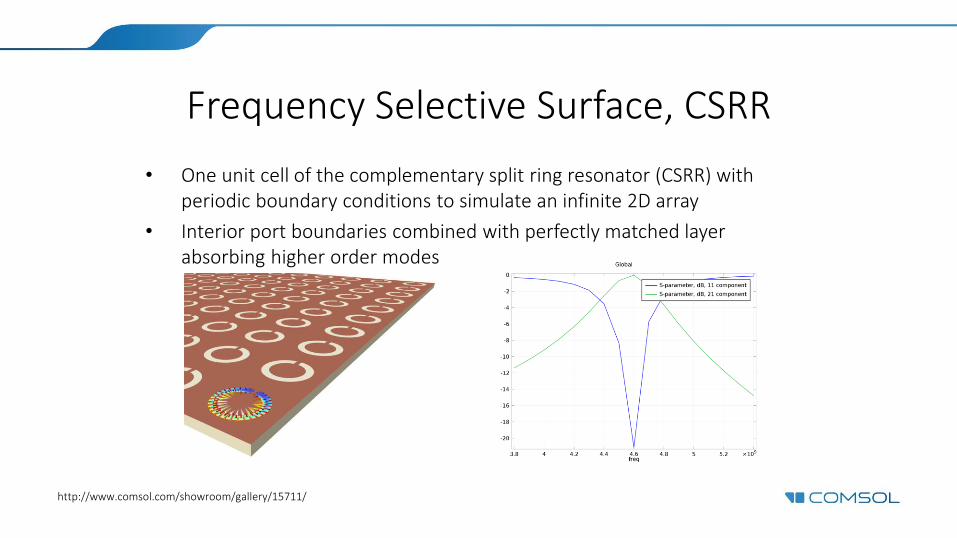
Frequency Selective Surface, CSRR
• One unit cell of the complementary split ring resonator (CSRR) with periodic boundary conditions to simulate an infinite 2D array
• Interior port boundaries combined with perfectly matched layer absorbing higher order modes
http://www.comsol.com/showroom/gallery/15711/

Frequency Selective Surface Simulator
• Periodic structures that generate a bandpass or a bandstop frequency response
• Built-in unit cell types: five popular FSS types, with two predefined polarizations and propagation at normal incidence
• The reflection and transmission spectra, the electric field norm on the top surface of the unit cell, and the dB-scaled electric field norm
http://www.comsol.com/showroom/gallery/24371/
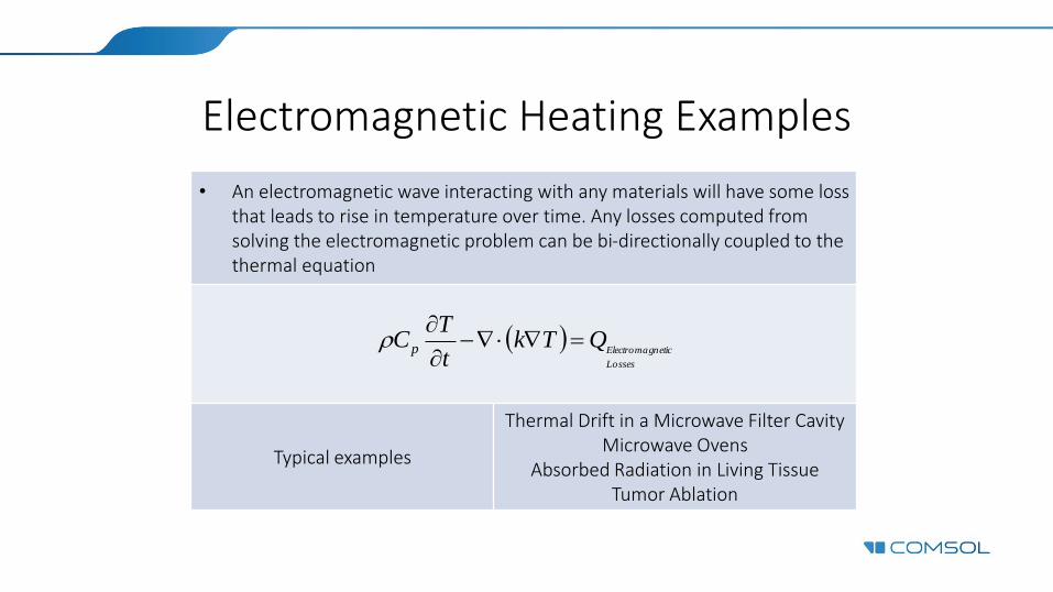
• An electromagnetic wave interacting with any materials will have some loss that leads to rise in temperature over time. Any losses computed from solving the electromagnetic problem can be bi-directionally coupled to the thermal equation
Typical examples
Thermal Drift in a Microwave Filter Cavity Microwave Ovens
Absorbed Radiation in Living Tissue Tumor Ablation
Electromagnetic Heating Examples
Losses
neticElectromagQTk
t
TCp
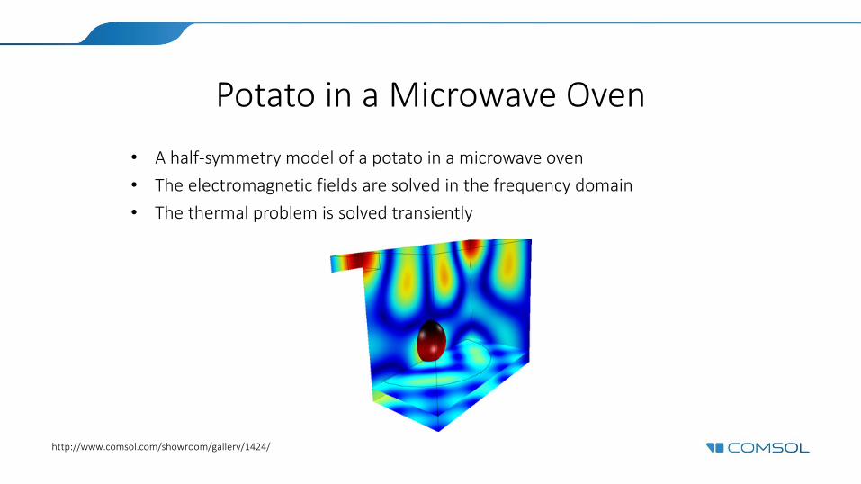
Potato in a Microwave Oven
• A half-symmetry model of a potato in a microwave oven
• The electromagnetic fields are solved in the frequency domain
• The thermal problem is solved transiently
http://www.comsol.com/showroom/gallery/1424/
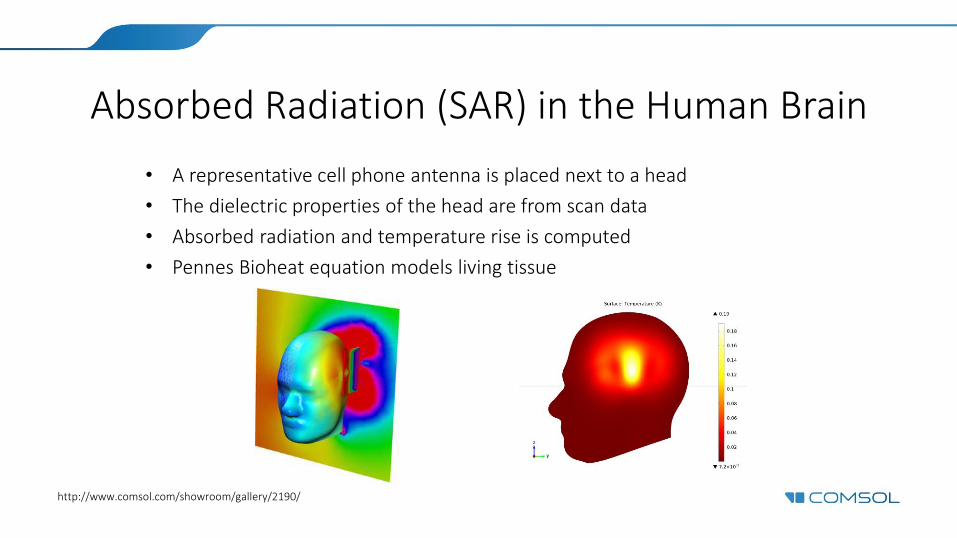
Absorbed Radiation (SAR) in the Human Brain
• A representative cell phone antenna is placed next to a head
• The dielectric properties of the head are from scan data
• Absorbed radiation and temperature rise is computed
• Pennes Bioheat equation models living tissue
http://www.comsol.com/showroom/gallery/2190/
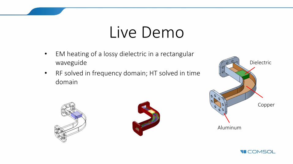
Live Demo • EM heating of a lossy dielectric in a rectangular
waveguide
• RF solved in frequency domain; HT solved in time domain
Aluminum
Copper
Dielectric

Contact Us
• Questions? www.comsol.com/contact
• www.comsol.com
– User Stories – Videos – Application Gallery – Discussion Forum – Blog – Product News


![[1314][ogx][gip] icps lead](https://static.fdocuments.net/doc/165x107/554c6919b4c905f76f8b4b6b/1314ogxgip-icps-lead.jpg)


![[1314][ogx] winter icps openning&lead&closing](https://static.fdocuments.net/doc/165x107/54543e28b1af9f99228b4902/1314ogx-winter-icps-openningleadclosing.jpg)