RF-powered internet of things - DRScj82kv96h/... · RF-Powered Internet of Things A Dissertation...
178
RF-Powered Internet of Things A Dissertation Presented by M. Yousof Naderi to The Department of Electrical and Computer Engineering in partial fulfillment of the requirements for the degree of Doctor of Philosophy in Computer Engineering Northeastern University Boston, Massachusetts December 2015
Transcript of RF-powered internet of things - DRScj82kv96h/... · RF-Powered Internet of Things A Dissertation...

RF-Powered Internet of Things
A Dissertation Presented
by
M. Yousof Naderi
to
The Department of Electrical and Computer Engineering
in partial fulfillment of the requirements
for the degree of
Doctor of Philosophy
in
Computer Engineering
Northeastern University
Boston, Massachusetts
December 2015

To my parents, Masoumeh and Gholamali,
for their endless love, encouragement, and support
ii

Contents
List of Figures vi
List of Tables ix
Acknowledgments x
Abstract of the Dissertation xi
1 Introduction 11.1 Research Challenges . . . . . . . . . . . . . . . . . . . . . . . . . . . . . . . . . 11.2 Organization and Contributions of the Thesis . . . . . . . . . . . . . . . . . . . . 2
2 Energy Harvesting Wireless Sensor Networks 52.1 Introduction . . . . . . . . . . . . . . . . . . . . . . . . . . . . . . . . . . . . . . 52.2 Node Platforms . . . . . . . . . . . . . . . . . . . . . . . . . . . . . . . . . . . . 6
2.2.1 Architecture of a Sensor Node with Harvesting Capabilities . . . . . . . . 62.2.2 Harvesting Hardware Models . . . . . . . . . . . . . . . . . . . . . . . . 72.2.3 Battery Models . . . . . . . . . . . . . . . . . . . . . . . . . . . . . . . . 10
2.3 Techniques of Energy Harvesting . . . . . . . . . . . . . . . . . . . . . . . . . . . 112.4 Prediction Models . . . . . . . . . . . . . . . . . . . . . . . . . . . . . . . . . . . 162.5 Protocols . . . . . . . . . . . . . . . . . . . . . . . . . . . . . . . . . . . . . . . 19
2.5.1 Task Allocation . . . . . . . . . . . . . . . . . . . . . . . . . . . . . . . . 192.5.2 Harvesting-aware Communication Protocols: MAC and Routing . . . . . . 25
2.6 Final Remarks . . . . . . . . . . . . . . . . . . . . . . . . . . . . . . . . . . . . . 31
3 Reliability Modeling of Energy Harvesting Sensor Nodes 333.1 Introduction . . . . . . . . . . . . . . . . . . . . . . . . . . . . . . . . . . . . . . 333.2 The SAVE Analytical Framework . . . . . . . . . . . . . . . . . . . . . . . . . . 34
3.2.1 Residual Energy Distribution . . . . . . . . . . . . . . . . . . . . . . . . . 363.2.2 Node Lifetime Distribution . . . . . . . . . . . . . . . . . . . . . . . . . . 40
3.3 Framework Analysis: A Case Study . . . . . . . . . . . . . . . . . . . . . . . . . 413.3.1 Semi-Markov Chain Overview . . . . . . . . . . . . . . . . . . . . . . . . 423.3.2 Constructing the SMP Kernel . . . . . . . . . . . . . . . . . . . . . . . . 43
3.4 Performance Evaluation . . . . . . . . . . . . . . . . . . . . . . . . . . . . . . . . 47
iii

3.5 Final Remarks . . . . . . . . . . . . . . . . . . . . . . . . . . . . . . . . . . . . . 49
4 Medium Access Control for Integrated Data and Energy Trasnfer 504.1 Introduction . . . . . . . . . . . . . . . . . . . . . . . . . . . . . . . . . . . . . . 504.2 Related Works . . . . . . . . . . . . . . . . . . . . . . . . . . . . . . . . . . . . . 52
4.2.1 General Energy Harvesting Sensor Networks . . . . . . . . . . . . . . . . 524.2.2 Sensor Networks with Wireless Energy Transfer . . . . . . . . . . . . . . 52
4.3 Design Challenges and Preliminary Experiments . . . . . . . . . . . . . . . . . . 534.3.1 Energy Interference and Cancellation . . . . . . . . . . . . . . . . . . . . 534.3.2 Optimal Frequency and Distance Separation . . . . . . . . . . . . . . . . . 554.3.3 Energy Charging Time . . . . . . . . . . . . . . . . . . . . . . . . . . . . 574.3.4 Requesting and Granting Energy . . . . . . . . . . . . . . . . . . . . . . . 574.3.5 Data vs. Energy Channel Access . . . . . . . . . . . . . . . . . . . . . . . 57
4.4 RF-MAC Protocol Overview . . . . . . . . . . . . . . . . . . . . . . . . . . . . . 574.4.1 Example Operation of RF-MAC . . . . . . . . . . . . . . . . . . . . . . . 59
4.5 Detailed RF-MAC Protocol Description . . . . . . . . . . . . . . . . . . . . . . . 604.5.1 Joint ET-spectrum Selection . . . . . . . . . . . . . . . . . . . . . . . . . 604.5.2 Adaptive Charging Threshold . . . . . . . . . . . . . . . . . . . . . . . . 644.5.3 Energy-aware Access Priority . . . . . . . . . . . . . . . . . . . . . . . . 65
4.6 Simulation Results . . . . . . . . . . . . . . . . . . . . . . . . . . . . . . . . . . 674.6.1 Impact of the Number of ETs . . . . . . . . . . . . . . . . . . . . . . . . 694.6.2 Impact of Multiple Flows . . . . . . . . . . . . . . . . . . . . . . . . . . . 704.6.3 Impact of the Number of Sensor Nodes . . . . . . . . . . . . . . . . . . . 714.6.4 Impact of Packet Size . . . . . . . . . . . . . . . . . . . . . . . . . . . . . 71
4.7 Experimental Study . . . . . . . . . . . . . . . . . . . . . . . . . . . . . . . . . . 724.8 Final Remarks . . . . . . . . . . . . . . . . . . . . . . . . . . . . . . . . . . . . . 75
5 Omnidirectional RF-Powered Wireless Sensor Network 785.1 Introduction . . . . . . . . . . . . . . . . . . . . . . . . . . . . . . . . . . . . . . 785.2 Concurrent Data and Wireless Energy Transfer . . . . . . . . . . . . . . . . . . . 78
5.2.1 Experimental Setup . . . . . . . . . . . . . . . . . . . . . . . . . . . . . . 805.2.2 Ranges for Coexistent WSNs and ETs . . . . . . . . . . . . . . . . . . . . 805.2.3 Concurrent Data and Energy Transmissions . . . . . . . . . . . . . . . . . 845.2.4 Concurrent Energy Transmissions: Same Frequency . . . . . . . . . . . . 865.2.5 Concurrent Energy Transmissions: Multi-Frequency . . . . . . . . . . . . 90
5.3 Surviving Wireless Energy Interference . . . . . . . . . . . . . . . . . . . . . . . 925.3.1 Experimental Platform and Methodology . . . . . . . . . . . . . . . . . . 945.3.2 Packet Reception Rate . . . . . . . . . . . . . . . . . . . . . . . . . . . . 955.3.3 Energy Interference . . . . . . . . . . . . . . . . . . . . . . . . . . . . . . 975.3.4 Temporal Change in Energy Interference . . . . . . . . . . . . . . . . . . 101
5.4 Energy Models and Analysis . . . . . . . . . . . . . . . . . . . . . . . . . . . . . 1025.4.1 2D RF Energy Model . . . . . . . . . . . . . . . . . . . . . . . . . . . . . 1035.4.2 3D RF Energy Model . . . . . . . . . . . . . . . . . . . . . . . . . . . . . 1065.4.3 Analysis and Simulation Results . . . . . . . . . . . . . . . . . . . . . . . 110
5.5 Final Remarks . . . . . . . . . . . . . . . . . . . . . . . . . . . . . . . . . . . . . 113
iv

6 Energy Harvesting from Direct RF Beamforming and Ambient Sources 1156.1 Introduction . . . . . . . . . . . . . . . . . . . . . . . . . . . . . . . . . . . . . . 115
6.1.1 Using Beamforming vs. Omnidirectional Radiation . . . . . . . . . . . . . 1156.1.2 A “cognitive” Approach to Ambient Energy Harvesting . . . . . . . . . . 1166.1.3 Dynamic and Anticipatory Energy Scheduling . . . . . . . . . . . . . . . 117
6.2 Architecture and System Operation . . . . . . . . . . . . . . . . . . . . . . . . . . 1186.2.1 Architecture Description . . . . . . . . . . . . . . . . . . . . . . . . . . . 1186.2.2 System Operation Overview . . . . . . . . . . . . . . . . . . . . . . . . . 119
6.3 HYDRA Functional Blocks . . . . . . . . . . . . . . . . . . . . . . . . . . . . . . 1206.3.1 ET Placement Optimization . . . . . . . . . . . . . . . . . . . . . . . . . 1216.3.2 Integrated Energy and Data Duty-cycling . . . . . . . . . . . . . . . . . . 1246.3.3 Adaptive Resource Allocation . . . . . . . . . . . . . . . . . . . . . . . . 132
6.4 Performance Evaluation . . . . . . . . . . . . . . . . . . . . . . . . . . . . . . . . 1336.4.1 Ambient RF Preliminary Experiments . . . . . . . . . . . . . . . . . . . . 1346.4.2 Optimal ET Placement Evaluation . . . . . . . . . . . . . . . . . . . . . . 1356.4.3 Adaptive Resource Allocation Evaluation . . . . . . . . . . . . . . . . . . 137
6.5 Related Works . . . . . . . . . . . . . . . . . . . . . . . . . . . . . . . . . . . . . 1426.6 Final Remarks . . . . . . . . . . . . . . . . . . . . . . . . . . . . . . . . . . . . . 143
7 Conclusion 146
Bibliography 148
v

List of Figures
2.1 System architecture of a wireless node with energy harvesters. . . . . . . . . . . . 72.2 General architecture of the energy subsystem of a wireless sensor node with energy
harvesting capabilities. . . . . . . . . . . . . . . . . . . . . . . . . . . . . . . . . 82.3 Different energy types (rectangles) and sources (ovals). . . . . . . . . . . . . . . . 112.4 Pro-Energy predictions. . . . . . . . . . . . . . . . . . . . . . . . . . . . . . . . . 192.5 ODMAC: data packet transmission. . . . . . . . . . . . . . . . . . . . . . . . . . 262.6 Overview of MTTP multi-tier EHWSN architecture. . . . . . . . . . . . . . . . . 27
3.1 A harvesting node as a semi-Markov process. . . . . . . . . . . . . . . . . . . . . 363.2 Semi-Markov Chain of a harvesting sensor node . . . . . . . . . . . . . . . . . . . 423.3 Probability density functions of net consumed energy for different operational cycles
n=10 and n=30. . . . . . . . . . . . . . . . . . . . . . . . . . . . . . . . . . . . . 473.4 Distribution of node lifetime with E0 = 10 Joules. . . . . . . . . . . . . . . . . . 48
4.1 Example network architecture with energy transmitters (x, y, z) and RF harvestingsensors (S1,S2). The energy transmitters can cancel emitted energy waves of eachothers (a). Phase difference effect on the received signal power at 915 MHz (b). . . 54
4.2 Effect of energy waves phase difference on the received signal power at different fre-quencies. The power of resulting wave drops significantly after π/2 phase separation(a). The scheme for two-tone wireless energy transfer (b). . . . . . . . . . . . . . . 56
4.3 Example scenario for overview of RF-MAC protocol with three RF energy harvestingsensor nodes. . . . . . . . . . . . . . . . . . . . . . . . . . . . . . . . . . . . . . 58
4.4 Five stages of joint ET-spectrum selection component in RF-MAC protocol. . . . . 594.5 Grouping and selection of ETs based on the destructive interference of energy waves
(a), the timing diagram for requesting and granting energy in the RF-MAC protocol (b). 604.6 Energy-aware data exchange process in RF-MAC protocol with three transmitter
nodes S1, S2, and S4 and the receiver node S3. . . . . . . . . . . . . . . . . . . . 674.7 Effect of the number of ETs on the average harvested energy. . . . . . . . . . . . . 694.8 Effect of the number of ETs on the average network throughput. . . . . . . . . . . 704.9 Effect of multiple flows on the average harvested energy. . . . . . . . . . . . . . . 714.10 Effect of multiple flows on the average network throughput. . . . . . . . . . . . . . 724.11 Effect of the number of nodes on the average harvested energy. . . . . . . . . . . . 734.12 Effect of the number of nodes on the average network throughput. . . . . . . . . . 74
vi

4.13 Effect of the packet size on the average harvested energy. . . . . . . . . . . . . . . 754.14 Effect of the packet size on the average network throughput. . . . . . . . . . . . . 764.15 Our fabricated RF energy harvester [1] powers Mica2 mote by converting the received
RF power to electrical energy. . . . . . . . . . . . . . . . . . . . . . . . . . . . . 764.16 Schematic of our experimental setup for transmission of wireless RF power. . . . . 774.17 Effect of ET2 position on the average harvested energy. . . . . . . . . . . . . . . . 774.18 Effect of ET2 position on the average network throughput. . . . . . . . . . . . . . 77
5.1 The wireless charging (C1), communication (C2) and interference (C3) ranges. . . 815.2 Charging ranges: experiments vs. theory. . . . . . . . . . . . . . . . . . . . . . . . 825.3 (a) Communication ranges for different data transmit powers. (a) Energy transmission
interference for different ET powers. (c) RSS for concurrent data and energy transferat the same frequency. . . . . . . . . . . . . . . . . . . . . . . . . . . . . . . . . . 82
5.4 The average PRR for varying energy transmission frequencies. . . . . . . . . . . . 855.5 The 95% confidence interval of PRR over different distances and frequencies. . . . 875.6 Multiple energy transmitters at the same frequency cancel transferred energy in
destructive areas and aggregate energy in constructive areas. . . . . . . . . . . . . 885.7 Effect of destructive and constructive energy interference for two ETs. The distance
between ET1 and the receiver is set to (a) 1 m, (b) 2 m, and (c) 3 m. . . . . . . . . 895.8 RF harvesting efficiency between the RF harvester and the ET for Powercast P2110
(a) and P1110 (b) harvesting boards. . . . . . . . . . . . . . . . . . . . . . . . . . 915.9 Effects of varying wireless ET frequencies on PRR (a) indoor and (b) outdoor. . . 955.10 Effects of ET distance on the PRR at gray, white, and black energy frequencies (a)
indoor and (b) outdoor. . . . . . . . . . . . . . . . . . . . . . . . . . . . . . . . . 955.11 Distribution of RSSI for energy interference indoor for varying ET frequencies in
gray, white, and black regions. . . . . . . . . . . . . . . . . . . . . . . . . . . . . 975.12 Distribution of RSSI for energy interference outdoor for varying ET frequencies in
gray, white, and black regions. . . . . . . . . . . . . . . . . . . . . . . . . . . . . 985.13 Effects of different ET distances on distributions of energy interference for (a) indoor
gray region, (b) outdoor gray region, and (c) outdoor white region. . . . . . . . . . 1005.14 Temporal characteristics of energy interference power in indoor (a, c, e) and outdoor
(b, d, f) environments for gray, black, and white frequency regions. . . . . . . . . . 1015.15 Two ETs transferring power on the same frequency to a receiver node at distance R1
and R2. . . . . . . . . . . . . . . . . . . . . . . . . . . . . . . . . . . . . . . . . 1045.16 Geometrical parameters of an ETn transferring wireless energy to a receiver at
far-field point M. . . . . . . . . . . . . . . . . . . . . . . . . . . . . . . . . . . . 1075.17 (a) Received power samples over the WSN space with 40 ETs. (b) Log-Normal
distributions of the network wide received power from multiple ETs. (c) Poweroutage probability based on CDF of the received power from multiple ETs. . . . . 108
5.18 (a) Comparison of received power with energy interference and without interference.(b) Energy interference samples over the sensor network with 40 ETs. (c) Log-Normal distributions of energy interference for multiple ETs. . . . . . . . . . . . . 111
5.19 (a) Dual-stage distributions of the harvested power (dBm) over the sensor networkwith different number of ETs. (b) Rayleigh distributions of the harvested voltageover the network. (c) CDFs of the harvested voltage over the network. . . . . . . . 112
vii

5.20 Intensity and patterns of harvested voltage. . . . . . . . . . . . . . . . . . . . . . . 113
6.1 HYDRA: Sensors are powered by ETs with beamforming capabilities and ambientenergy sources. . . . . . . . . . . . . . . . . . . . . . . . . . . . . . . . . . . . . 116
6.2 Functional blocks for HYDRA. . . . . . . . . . . . . . . . . . . . . . . . . . . . . 1206.3 Model of data and energy duty-cycle planes. RF energy harvesting follows Eintrv
duty-cycling and data communications have the offered traffic rate Tdc over Dintrv. 1216.4 Calculating time-varying total traffic rate at each node based on the given active
paths and local traffic rates. . . . . . . . . . . . . . . . . . . . . . . . . . . . . . 1256.5 The sequence of energy beams and durations over a data interval at sensor Si. Each
traffic update duration consists of multiple data interval and each data intervalsconsists of multiple energy epochs. . . . . . . . . . . . . . . . . . . . . . . . . . . 126
6.6 Depicting the energy-in-advance transfer policy for maximizing the harvested power,minimizing energy dissipation from ETs, and load balancing. . . . . . . . . . . . . 131
6.7 The optimal number of ETs in the HYDRA planning phase for different offeredloads, number of nodes, and ambient powers. . . . . . . . . . . . . . . . . . . . . 136
6.8 Comparing HYDRA planning with random placed beamforming and omnidirectionalschemes for N=10 and Pamb equals to (a) 0.0362 mW, (b) 0.0821 mW. . . . . . . . 138
6.9 Optimal number of ETs is shown for varying number of ET transmission power,number of nodes, and ambient power. . . . . . . . . . . . . . . . . . . . . . . . . 139
6.10 Comparing HYDRA variants and static beamforming for varying packet input ratesover entire simulation time. . . . . . . . . . . . . . . . . . . . . . . . . . . . . . . 140
6.11 Effect of different event interval rates for HYDRA variants and static beamformingover network simulation time. . . . . . . . . . . . . . . . . . . . . . . . . . . . . 141
6.12 Effect of different number of sensors on the performance of HYDRA for three setsof α and γ. . . . . . . . . . . . . . . . . . . . . . . . . . . . . . . . . . . . . . . 142
viii

List of Tables
2.1 Comparison of MAC protocols for EHWSNs. . . . . . . . . . . . . . . . . . . . . 282.2 Comparison of power density and efficiency of different energy harvesting techniques 32
3.1 Parameters of SAVE Framework for the case study . . . . . . . . . . . . . . . . . 41
4.1 Parameters used in RF-MAC . . . . . . . . . . . . . . . . . . . . . . . . . . . . . 66
5.1 Summary of measured coexistence ranges in wireless-powered sensor network. . . 845.2 Energy spectral ranges in concurrent energy and data transmission. . . . . . . . . . 875.3 Map of energy interference power and associated PRR. . . . . . . . . . . . . . . . 99
6.1 Important Symbols Used for HYDRA Description . . . . . . . . . . . . . . . . . . 1446.2 HYDRA simulation parameters in ns-2. . . . . . . . . . . . . . . . . . . . . . . . 1456.3 Summary of Boston ambient RF power measurements over 40 subway stations. . . 145
ix

Acknowledgments
Working towards a Ph.D. has been a deeply enriching and rewarding experience for me.Looking back, it becomes obvious to me many people have helped shape this journey. In the limitedspace I have here, I would like to extend them my thanks.
First and foremost, I would like to thank my advisors Dr. Kaushik Chowdhury and Dr.Stefano Basagni for supporting me over the years. My work would not have been possible withouttheir constant guidance and unwavering encouragement. I am grateful to them for putting their trustin me, and for providing valuable insights, suggestions, resources, and opportunities of all kindsin order for me to pursue my passions and conduct research throughout my PhD. I have been veryfortunate to have had advisors who taught me not only how to research and be innovative but alsomany life lessons through their experience and our interaction. Over and above our research, I havelearnt about the power of collaboration and balance, how you should remain true to your passions,constant focus on outcomes and creating value, setting right priorities in life, and the careful craftingof even the simplest assignments. For all of your support, inspiration, and teachings, Kaushik andStefano, thank you.
I am also grateful to Dr. Tommaso Melodia for agreeing to be on my defense committee aswell as his excellent advice and feedback that have been invaluable.
Also, I have been fortunate to work closely with some wonderful colleagues and peersoutside Northeastern University, both here in the United States and from India, Italy, and Spain. Iwould like to thank Dr. Wendi Heinzelman from University of Rochester, Dr. Swades De and Dr.Soumya Jana from Indian Institute of Technology, India, Dr. Chiara Petrioli and Dora Spenza fromUniversit‘a di Roma ”La Sapienza” Roma, Italy, and Raul G. Cid-Fuentes, Dr. Albert Cabellos-Aparicio, and Dr. Eduard Alarcon from Universitat Politecnica de Catalunya, Spain, with all ofwhom I have enjoyed collaborating on different projects.
I am thankful to all the members of the Next GEneration NEtworks and SYStems(GENESYS) Lab, both past and present, for the help they provided during my research, and alsofor their support and encouragement. I would specifically thank Dr. Prusayon Nintanavongsa, Dr.Rahman Doost, and Ufuk Muncuk, who have served as my collaborators and friends over the pastfew years, and with whom I have had fruitful discussions on different parts of this dissertation.
Last but not least, I would like to thank my family, Masoumeh and Gholamali. You raisedme, loved me, taught me right from wrong, and gave me all that I needed. This is dedicated to youwith love.
x

Abstract of the Dissertation
RF-Powered Internet of Things
by
M. Yousof Naderi
Doctor of Philosophy in Computer Engineering
Northeastern University, December 2015
Dr. Kaushik Chowdhury& Dr. Stefano Basagni, Advisers
Wireless charging through directed radio frequency (RF) waves and ambient RF energysources is an attractive solution to power small wireless devices. RF-based wireless charging canpotentially realize battery-less sensor networks and eliminate the need for external power cables orperiodic battery replacements. However, the coexistence of data communication and energy comes atthe cost of new challenges, which this research tackles holistically through a combination of systemlevel design, experimentation, analysis and protocol formulation.
First, a stochastic tool for analyzing nodal residual energy and lifetime distribution isproposed. Our analytical framework models an energy harvesting sensor as a stochastic semi-Markovprocess and introduces a new analysis technique, called energy transient analysis. The frameworkreturns, with fine granularity, the energy consumed during various protocol-related functions, as wellas the incoming energy via harvesting. As a second contribution, the opportunities and challenges ofRF energy harvesting are identified through extensive practical testing. This study lays out essentialnetwork design guidelines for separating energy transmitter (ET) operations and those of the RFenergy harvesting nodes in the spatio-temporal and frequency domains. It also examines the energyinterference among concurrent RF waves that may result in destructive combinations of the net signalenergy if the ETs are randomly placed. To verify the experimental findings, a set of closed formequations for omni-directional ETs is developed that accurately captures the locations where the ETaction is cumulative. Next, a medium access control called RF-MAC is designed for ET and sensorcoordination that jointly selects energy transmitters and their frequencies based on the collectiveimpact on charging time and energy interference, sets the maximum energy charging threshold,requests and grants energy, and decides the access priority of both data and energy.
Finally, a planning and network resource management framework for powering smallform factor sensor node called HYDRA is introduced that uses distributed ad hoc beamforming-capable ETs and leverages cognitive ambient energy harvesting from cellular and TV spectrum bands.
xi

HYDRA proposes a new strategy for supplying energy called energy-in-advance transfer (EIA)which provides nodes in advance with the energy they will need for current and future operations. Inthe planning phase, it determines the locations of ETs that jointly maximizes energy from ambientsources and minimizes the number of ETs to reduce costs and overhead. In the resource managementphase, through novel mathematical formulations for optimal radiating power levels and phases ofthe ETs, HYDRA determines the spatial scheduling of the energy beams mapping ET operationsto changing network requirements and available ambient energy, while minimizing the energyexpenditures of ETs.
The results of this work can all be integrated to address real-world wireless poweredsystems, such as the design of the next generation RF-powered Internet of Things (IoT).
xii

Chapter 1
Introduction
Wireless Sensor Networks (WSNs) are a fundamental building block of the Internet of
Things (IoT) and a key enabler for cyber physical and pervasive computing systems. However, sensor
nodes are typically battery-powered, and their limited energy affects protocol design, sacrificing
throughput, bandwidth usage, and reliability to the need for extended network lifetime through
judicious use of energy. Since it is often difficult, if not impossible, to access the sensor nodes and
replace their batteries, most research efforts have focused on intelligent duty cycling and energy
saving techniques at all layers of the protocol stack. Recent developments in energy harvesting
technology from ambient sources promise to alleviate some of these concerns. Among sources of
energy, electromagnetic waves carry energy in the form of electric and magnetic fields, which can be
converted (with some losses) and stored as energy at the receiving front-end, and used to power the
processing and communication circuits of the nodes of a wireless sensor network (WSN). The ability
of transferring energy via contact-less radio frequency (RF) will ensure the sensor nodes to remain
operational for long times, without the need of costly battery replacement efforts.
1.1 Research Challenges
Sensor nodes powered by rechargeable batteries would replenish through energy scavenged
from controlled or ambient sources. Such a charging paradigm extends the network lifetime by
reducing the charge drawn from the battery, prevents disruptions owing to battery replacement, and
ensures environmentally friendly operation. However, as the residual energy at the node is time
varying, and is subject to a variety of other factors, it is a challenge for the network designer to
formulate closed form expressions that indicate future energy levels and lifetime of a EHWSN node.
1

CHAPTER 1. INTRODUCTION
Moreover, current prototypes of RF transfer have limited charging range (few meters) and
efficiency (40 to 60%). This imposes the concurrent and coordinated use of multiple ETs to power
an entire WSN. While multiple ETs are needed to ensure high energy transfer rates, they introduce
interference among RF waves from different ETs, leading to significant and various constructive
and destructive combinations over the network deployment area. Being able to compute the energy
harvestable at a given point in space is a non-trivial task, as it depends on the relative locations of
active ETs, path loss information, and on the different distances from the ETs and a receiver at that
point.
The integration of data and energy communications also results into several challenges at
the protocol level such as: (i) how and when should the energy transfer occur, (ii) its priority over,
and the resulting impact on the process of data communication, (iii) the challenges in aggregating the
charging action of multiple transmitters, and (iv) impact of the choice of frequency. Thus, the act of
energy transfer becomes a complex medium access problem, which must embrace a cross-disciplinary
approach incorporating wave propagation effects and device characteristics, apart from the classical
link layer problem of achieving fairness in accessing the channel.
While ambient energy harvesting has the advantage of scavenging existing pervasive
radiation without any need of dedicated transmitter, its power density is subject to the surrounding
environments, schedule followed by the base stations and mobile users, underlying dynamic channel
characteristics, the line of sight, and distance to the ambient sources. Moreover, the wireless power
transfer can be carefully controlled through dedicated ETs, though this needs distributed coordination
among multiple ETs, energy load distribution, adaptive power control and scheduling of energy
transmissions based on the dynamic traffic and energy requirements of the sensor nodes for effective
energy transfer.
In this dissertation in order to address these problems we propose a set of analytical
frameworks, communication protocols, and resource allocation algorithms along comprehensive
simulations and experimental studies.
1.2 Organization and Contributions of the Thesis
Chapter 2 explores the opportunities and challenges of energy harvesting wireless sensor
networks (EHWSNs), explaining why the design of protocol stacks for traditional WSNs has to be
radically revisited. It describes the architecture of a EHWSN node, and especially that of its energy
subsystem and presents the various forms of energy that are available and ways for harvesting them.
2

CHAPTER 1. INTRODUCTION
Models for predicting availability of energy as well as task allocation, MAC and routing protocols
are discussed.
Chapter 3 introduces a stochastic tool called SAVE, Stochastic Analysis and aVailability of
Energy, for the analysis of the residual energy and the lifetime distribution of nodes. It models the
energy harvesting wireless sensor node as a stochastic semi-Markov process and introduce a new
analysis technique, called energy transient analysis, for the computation of the net consumed energy
distribution. The amount of consumed and harvested energy in each state of a node are modeled as
random variables, depending on discharging and recharging rates and on the holding time distribution
of that state. SAVE captures a wide umbrella of input factors through its kernel, including channel
characteristics, different energy sources and harvesting policies, link layer parameters (e.g., error
control and duty cycling) and data traffic generation models.
Chapter 4 proposes a medium access control for integrated data and energy transfer. It
addresses the problems of the joint selection of energy transmitters and their frequencies based on the
collective impact on charging time and energy interference, setting the maximum energy charging
threshold, requesting and granting energy, and energy-aware access priority. It optimizes energy
delivery to sensor nodes, while minimizing disruption to data communication. The grouping of
the ETs into two sets with varying transmission frequencies, and the minimal control overhead are
both geared to keep the hardware requirements simple, and the protocol easier to implement. Both
simulation and experimental testbed results provide the performance of this protocol in terms of the
average harvested energy and average network throughput.
Chapter 5 studies the omnidirectional RF-powered wireless sensor network and propose
analytical models to capture the behavior and energy interference in such networks. In particular, it
first provides the experimental study to quantify the rate of charging, packet loss due to interference,
and suitable ranges for charging and data communication of the ETs. It explores how the placement
and relative distances of multiple ETs affect the charging process, demonstrating constructive and
destructive energy aggregation at the sensor nodes. In addition, it investigates the impact of the
separation in frequency between data and energy transmissions, as well as among multiple concurrent
energy transmissions, and demonstrates how separating the energy and data transfer gives rise to
black (high loss), gray (moderate loss), and white (low loss) regions with respect to packet errors.
Then it shows safe frequency separation for concurrent data and energy transmission and measures
the impact of energy cancellation on the amount of harvested power. Finally, chapter 5 introduces
closed form expressions of the energy harvestable at any point in the deployment space of the WSN
capturing low-power data communications, RF energy harvesting circuit, and interference among
3

CHAPTER 1. INTRODUCTION
energy signals.
Chapter 6 proposes a planning and resource management framework for jointly harvesting
RF energy from directional beams and ambient sources. It first introduces a mathematical model
for the task of optimal ET placement that jointly optimizes direct and ambient energy harvesting.
Furthermore, it formulates strategies for dynamically adjusting the transmission power and phase
of the ETs and for determining the spatial scheduling of the energy beams, mapping ET energy
provisioning to the changing demands of the nodes while considering available ambient energy and
minimizing the energy expenditures of ETs. To this end, it formalizes the necessary traffic and energy
models for the nodes based on the volume of transferred data. Moreover, it proposes a new strategy
for supplying energy called energy-in-advance transfer that provides nodes with the energy they
will need for current and future operations, while minimizing the power from the ETs. It leverages
the hardware-centric properties of typical RF harvesting circuits and strict convexity of harvested
power as a function of input power. Then the potential and benefits of cognitive ambient RF energy
harvesting are demonstrated through a set of experiments conducted in Boston subway stations
for digital TV, and the 3G, GSM, and LTE bands. Finally, the proposed models, algorithms, and
framework are evaluated through comprehensive network simulations.
Chapter 7 draws the main conclusions of this thesis and outline future research directions.
4

Chapter 2
Energy Harvesting Wireless Sensor
Networks
2.1 Introduction
Wireless Sensor Networks (WSNs) have played a major role in the research field of
multi-hop wireless networks as enablers of applications ranging from environmental and structural
monitoring to border security and human health control. Research within this field has covered a
wide spectrum of topics, leading to advances in node hardware, protocol stack design, localization
and tracking techniques and energy management [2].
Research on WSNs has been driven (and somewhat limited) by a common focus: Energy
efficiency. Nodes of a WSN are typically powered by batteries. Once their energy is depleted, the
node is “dead.” Only in very particular applications batteries can be replaced or recharged. However,
even when this is possible, the replacement/recharging operation is slow and expensive, and decreases
network performance. Different techniques have therefore been proposed to slow down the depletion
of battery energy, which include power control and the use of duty cycle-based operation. The
latter technique exploits the low power modes of wireless transceivers, whose components can be
switched off for energy saving. When the node is in a low power (or “sleep”) mode its consumption
is significantly lower than when the transceiver is on. However, when asleep the node cannot transmit
or receive packets. The duty cycle expresses the ratio between the time when the node is on and the
sum of the times when the node is on and asleep. Adopting protocols that operate at very low duty
cycles is the leading type of solution for enabling long lasting WSNs [3]. However, this approach
5

CHAPTER 2. ENERGY HARVESTING WIRELESS SENSOR NETWORKS
suffers from two main drawbacks. 1) There is an inherent tradeoff between energy efficiency (i.e.,
low duty cycling) and data latency, and 2) battery operated WSNs fail to provide the needed answer
to the requirements of many emerging applications that demand network lifetimes of decades or
more. Battery leakage depletes batteries within a few years even if they are seldom used [4, 5]. For
these reasons recent research on long-lasting WSNs is taking a different approach, proposing energy
harvesters combined with the use of rechargeable batteries and super capacitors (for energy storage)
as the key enabler to “perpetual” WSN operations.
Energy Harvesting-based WSNs (EHWSNs) are the result of endowing WSN nodes with
the capability of extracting energy from the surrounding environment. Energy harvesting can exploit
different sources of energy, such as solar power, wind, mechanical vibrations, temperature variations,
magnetic fields, etc. Continuously providing energy, and storing it for future use, energy harvesting
subsystems enable WSN nodes to last potentially for ever.
This chapter explores the opportunities and challenges of EHWSNs, explaining why the
design of protocol stacks for traditional WSNs has to be radically revisited. We start by describing
the architecture of a EHWSN node, and especially that of its energy subsystem (Section 2.2). We
then present the various forms of energy that are available and ways for harvesting them (Section 2.3).
Models for predicting availability of wind and solar energy are described in Section 2.4. We then
survey task allocation, MAC and routing protocols proposed so far for EHWSNs in Section 2.5.
Conclusions are drawn in Section 6.6
2.2 Node platforms
EHWSNs are composed of individual nodes that in addition to sensing and wireless
communications are capable of extracting energy from multiple sources and converting it into usable
electrical power. In this section we describe in details the architecture of a wireless sensor node with
energy harvesting capabilities, including models for the harvesting hardware and for batteries.
2.2.1 Architecture of a Sensor Node with Harvesting Capabilities
An EHWSN platform typically consists of one or more energy harvesting boards (the
harvesters) attached to the wireless sensor node (Figure 2.1). The harvesting board uses one or more
energy harvesting techniques and is responsible for capturing and converting the external energy into
electrical power and for storing it.
6

CHAPTER 2. ENERGY HARVESTING WIRELESS SENSOR NETWORKS
External
Energy
Source(s)
Energy Harvester(s) Power Management
A/D ConverterLow Power
Microcontroller Unit
Low Power RF
Transceiver
Energy Storage
Sensor(s)
Memory
Figure 2.1: System architecture of a wireless node with energy harvesters.
The system architecture of a wireless sensor node includes the following components: 1)
The energy harvester(s), in charge of converting external ambient or human-generated energy to
electricity; 2) a power management module, that collects electrical energy from the harvester and
either stores it or delivers it to the other system components for immediate usage; 3) energy storage,
for conserving the harvested energy for future usage; 4) a microcontroller, for communication control
and other functions; 5) a radio transceiver, for transmitting and receiving information; 6) sensory
equipment, for sensing; 7) an A/D converter to digitize the analog signal generated by the sensors
and makes it available to the microcontroller for further processing, and 8) memory to store sensed
information, application-related data, and code.
In the next section we focus on the energy harvesting components (the energy subsystem)
of a EHWSN node, describing abstractions that have been proposed for modeling them.
2.2.2 Harvesting Hardware Models
The general architecture of the energy subsystem of a wireless sensor node with energy
harvesting capabilities is shown in Figure 2.2.
The energy subsystem includes one or multiple harvesters that convert energy available
from the environment to electrical energy. The energy obtained by the harvester may be used to
directly supply energy to the node or it may be stored for later use. Although in some application it is
possible to directly power the sensor node using the harvested energy (Harvest-use architecture [6]),
in general this is not a viable solution: The energy source needs to be available when the device is
operational, which can be an unrealistic assumption.
A more reasonable architecture enables the node to directly use the harvested energy, but
also includes a storage component that acts as an energy buffer for the system, with the main purpose
7

CHAPTER 2. ENERGY HARVESTING WIRELESS SENSOR NETWORKS
Energy Harvesters
PV cell
Wind turbin
RF
Storage
Power Conditioning Battery Manager
Energy Predictor
Power Manager
Loaddirect supply
......
Figure 2.2: General architecture of the energy subsystem of a wireless sensor node with energy
harvesting capabilities.
of accumulating and preserving the harvested energy. When the harvesting rate is greater than the
current usage, the buffer component can store excess energy for later use (e.g., when harvesting
opportunities do not exist), thus supporting variations in the power level emitted by the environmental
source.
The two alternatives commonly used for energy storage are secondary rechargeable
batteries and supercapacitors (also known as ultracapacitors). Supercapacitors are similar to regular
capacitors, but they offer very high capacitance in a small size. They offer several advantages with
respect to rechargeable batteries [7]. First of all, supercapacitors can be recharged and discharged
virtually an unlimited number of times, while typical lifetimes of an electrochemical battery is less
than 1000 cycles [4]. Second, they can be charged using simple charging circuits, thus reducing
system complexity, and do not need full-charge nor deep-discharge protection circuits. They also
have higher charging and discharging efficiency than electrochemical batteries [7]. Finally, due
to high power density, they can be charged quickly. Another additional benefit is the reduction of
environmental issues related to battery disposal. The major limitations of ultracapacitors are the
lower energy density and the higher self-discharge with respect to electrochemical batteries. They
also experience linear discharge, which makes them unable to deliver the full charge. However,
the leakage effect can be compensated quite well in case of solar energy harvesting, due to the
periodic and unlimited nature of this power source [8]. Thanks to this characteristics, many platforms
with harvesting capabilities use supercapacitors as energy storage, either by themselves [9, 10] or
in combination with batteries [11, 12, 13]. Other systems, instead, focus on platforms using only
rechargeable batteries [14, 15, 16].
8

CHAPTER 2. ENERGY HARVESTING WIRELESS SENSOR NETWORKS
Real energy storage devices, such as supercapacitors and rechargeable batteries, deviate
from ideal energy buffers in a number of ways: They have a finite size BMax and can hold a finite
amount of energy; they have a charging efficiency ηc < 1 and a discharging efficiency ηd < 1, i.e.,
some energy is lost while charging and discharging the buffer, and they suffer from leakage and
self-discharge, i.e., some stored energy is lost even if the buffer is not in use. Leakage and self-
discharge are phenomenons that affect both batteries and supercapacitors. All batteries suffer from
self-discharge: A cell that simply sits on the shelf, without any connection between the electrodes,
experiences a reduction in its stored charge due to internal chemical reactions, at a rate depending
on the cell chemistry and the temperature. A similar phenomenon affects electrochemical super-
capacitors in charged state. They suffer gradual loss of energy and reduction of the inter-plate
voltage.
Considering leakage current is important while dealing with energy harvesting systems,
especially if the application scenario requires the harvested energy to be stored for long periods
of time. In general, if the energy source is sporadic or if it is only able to provide a small amount
of energy, the portion of the harvested energy lost due to leakage may be significant. The leakage
is of particular relevance for supercapacitors, because their energy density is about one orders of
magnitude lower than that of an electrochemical battery, but they suffer from considerably higher self-
discharge. A supercapacitor leakage is strongly variable and depends on several factors, including
the capacitance value of the supercapacitor, the amount of energy stored, the operating temperature,
the charge duration, etc. For this reason, the leakage pattern of a particular supercapacitor must often
be determined experimentally [12, 17, 18, 7]. Additionally, the leakage current varies with time: It is
considerably higher immediately after the supercapacitor has been charged, then it decreases to a
plateau.
Several model for the leakage from a charged supercapacitor have been proposed in the
literature, modeling the leakage as a constant current [19], or as an exponential function of the
current supercapacitor voltage [20], or by using a polynomial approximation of its empirical leakage
pattern [18], or, finally, by using a piecewise linear approximation of its empirical leakage pattern [7].
Another aspect to consider in the supercapacitors vs. battery comparison is that in many application
scenarios it is not possible to use the full energy stored in the supercapacitor. The voltage of a
supercapacitor drops from full voltage to zero linearly, without the flat curve that is typical of most
electrochemical batteries. The fraction of the charge available to the sensor node depends on the
voltage requirements of the platform. For example, a Telos B mote requires a minimal voltage
ranging from 1.8 V to 2.1 V. When the supercapacitor voltage drops below this threshold, its residual
9

CHAPTER 2. ENERGY HARVESTING WIRELESS SENSOR NETWORKS
energy can no longer be used to power the node. This aspect may be partially mitigated by using
a DC-DC converter to increase the voltage range, at the cost of introducing inefficiencies and an
additional source of power consumption.
In order to reduce the energy lost trough buffer inefficiencies, many platforms allow the
node to directly use the energy harvested. In particular, if the current energy consumption is greater
or equal than the energy currently harvested, then the node can use the harvested energy for its
operations. This is the most efficient way of using the environmental energy, because it is used
directly and there is no energy loss. Otherwise, if the amount of energy harvested is greater than
the current energy consumption, some energy is directly used to sustain the node operations, while
excess energy is stored in the buffer for later use.
2.2.3 Battery Models
Many existing network simulators provide very simple battery models. Batteries are seen
as ideal energy storage devices and are modeled as containers of finite capacity, containing a certain
amount of energy units. Executing a network operation, e.g., sending or receiving a packet, uses
a certain amount of energy units, depending on the energy cost of the operation. Real batteries,
however, operate differently. As mentioned earlier, all batteries suffer from self-discharge. Even a cell
that is not being used experience a charge reduction caused by internal chemical activity. Batteries
also have charge and discharge efficiency strictly < 1, i.e., some energy is lost when charging and
discharging the battery. Additionally, batteries have some non-linear properties [4, 21, 22]. These
are: Rate-dependent capacity, i.e., the delivered capacity of a battery decreases, in a non-linear
way, as the discharge rate increases; temperature effect, in that the operating temperature affects the
battery discharge behavior and directly impact the rate of self-discharge; recovery effect, for which
the lifetime and the delivered capacity of a battery increases if discharge and idle periods alternate
(pulse discharge). Furthermore, rechargeable batteries experience a reduction of their capacity at
each recharge cycle, and their voltage depends on the charging level of the battery and varies during
discharge. These characteristics should be taken into account when dimensioning and simulating
energy harvesting systems, because they can easily lead to wrong estimations of the battery lifetime.
For example, if the harvesting subsystem uses a rechargeable battery to store the energy harvested
from the environment, it is important to consider that the reduction in capacity experienced by the
battery at each recharge cycle is likely to reduce both its delivered capacity and its lifetime.
Many types of battery models have been proposed recently in the literature [22]. These
10

CHAPTER 2. ENERGY HARVESTING WIRELESS SENSOR NETWORKS
Figure 2.3: Different energy types (rectangles) and sources (ovals).
include: Physical models that simulate the physical processes that take place into an electrochemical
battery. These models are usually very accurate, but have high computational complexity and require
high configuration effort [23, 24]. Empirical models that approximate the discharge behavior of a
battery with simple equations. They are generally the least accurate. However, they require low
computational resources and configuration effort [25, 26]. Abstract models that emulate battery
behavior by using simplified equivalent representation, such as stochastic system [27], electrical-
circuit models [28, 29], and discrete-time VHDL specification [30], and mixed models that use both
a high-level representation of a battery (simpler than a real battery) and analytical expressions based
on low-level analysis and physical laws [31].
2.3 Techniques of Energy Harvesting
Figure 2.3 shows the variety of energy types that can be harvested. In this section we
provide their brief description and relevant references.
Mechanical energy harvesting indicates the process of converting mechanical energy into electricity
by using vibrations, mechanical stress and pressure, strain from the surface of the sensor, high-
pressure motors, waste rotational movements, fluid, and force. The principle behind mechanical
energy harvesting is to convert the energy of the displacements and oscillations of a spring-mounted
mass component inside the harvester into electrical energy [32, 33]. Mechanical energy harvesting
can be: Piezoelectric, electrostatic and electromagnetic.
11

CHAPTER 2. ENERGY HARVESTING WIRELESS SENSOR NETWORKS
Piezoelectric energy harvesting is based on the piezoelectric effect for which mechan-
ical energy from pressure, force or vibrations is transformed into electrical power by straining a
piezoelectric material. The technology of a piezoelectric harvester is usually based on a cantilever
structure with a seismic mass attached into a piezoelectric beam that has contacts on both sides of
the piezoelectric material [33]. In particular, strains in the piezoelectric material produce charge
separation across the harvester, creating an electric field, and hence voltage, proportional to the stress
generated [34, 35]. Voltage varies depending on the strain and time, and an irregular AC signal is
produced. Piezoelectric energy conversion has the advantage that it generates the desired voltage
directly, without need for a separate voltage source. However, piezoelectric materials are breakable
and can suffer from charge leakage [36, 37, 33]. Examples of piezoelectric energy harvesters can be
found in [38, 39, 40, 41, 42] and references therein.
The principle of electrostatic energy harvesting is based on changing the capacitance of a
vibration dependent variable capacitor [43, 44]. In order to harvest the mechanical energy a variable
capacitor is created by opposing two plates, one fixed and one moving, and is initially charged.
When vibrations separate the plates, mechanical energy is transformed into electrical energy from
the capacitance change. This kind of harvesters can be incorporated into microelectronic-devices due
to their integrated circuit-compatible nature [45]. However, an additional voltage source is required
to initially charge the capacitor [37]. Recent efforts to prototype sensor-size electrostatic energy
harvesters can be found in [46, 47].
Electromagnetic energy harvesting is based on Faraday’s law of electromagnetic induction.
An electromagnetic harvester uses an inductive spring mass system for converting mechanical energy
to electrical. It induces voltage by moving a mass of magnetic material through a magnetic field
created by a stationary magnet. Specifically, vibration of the magnet attached to the spring inside a coil
changes the flux and produces an induced voltage [43, 33, 34]. The advantages of this method include
the absence of mechanical contact between parts and of a separate voltage source, which improves
the reliability and reduce the mechanical damping in this type of harvesters [36, 44]. However, it is
difficult to integrate them in sensor nodes because of the large size of electromagnetic materials [36].
Some examples of electromagnetic energy harvesting systems are presented in [48, 49].
Photovoltaic energy harvesting is the process of converting incoming photons from sources such
as solar or artificial light into electricity. Photovoltaic energy can be harnessed by using photovoltaic
(PV) cells. These consist of two different types of semiconducting materials called n-type and p-type.
An electrical field is formed in the area of contact between these two materials, called the P-N junction.
Upon exposure to light a photovoltaic cell releases electrons. Photovoltaic energy conversion is a
12

CHAPTER 2. ENERGY HARVESTING WIRELESS SENSOR NETWORKS
traditional, mature, and commercially established energy-harvesting technology. It provides higher
power output levels compared to other energy harvesting techniques and is suitable for larger-scale
energy harvesting systems. However, its generated power and the system efficiency strongly depend
on the availability of light and on environmental conditions. For example, in outdoor environment
power densities up to 100mW/cm2 are available, while indoor power levels are between 100 to
1000µW/cm2 [6, 50]. Other factors, including the materials used for the photovoltaic cell, affect
the efficiency and level of power produced by photovoltaic energy harvesters [36, 16]. Some recent
prototypes of photovoltaic harvesters are described in [51, 52, 53, 54]. Known implementations of
solar energy harvesting sensor nodes include Fleck [55], Enviromote [56], Trio [11], Everlast [10],
and Solar Biscuit [57].
Thermal energy harvesting is implemented by thermoelectric energy harvesting and pyroelectric
energy harvesting.
Thermoelectric energy harvesting is the process of creating electric energy from tem-
perature difference (thermal gradients) using thermoelectric power generators (TEGs). The core
element of a TEG is a thermopile formed by arrays of two dissimilar conductors, i.e., a p-type and
n-type semiconductor (thermocouple), placed between a hot and a cold plate and connected in series.
A thermoelectric harvester scavenges the energy based on the Seebeck effect, which states that
electrical voltage is produced when two dissimilar metals joined at two junctions are kept at different
temperatures [58]. This is because the metals respond differently to the temperature difference,
creating heat flow through the thermoelectric generator. This produces a voltage difference that is
proportional to the temperature difference between the hot and cold plates. The thermal energy is
converted into electrical power when a thermal gradient is created. Energy is harvested as long as the
temperature difference is maintained.
Pyroelectric energy harvesting is the process of generating voltage by heating or cooling
pyroelectric materials. These materials do not need a temperature gradient similar to a thermocouple.
Instead, they need time-varying temperature changes. Changes in temperature modify the locations
of the atoms in the crystal structure of the pyroelectric material, which produces voltage. To keep
generating power, the whole crystal should be continuously subject to temperature change. Otherwise,
the produced pyroelectric voltage gradually disappears due to leakage current [59].
Pyroelectric energy harvesting achieves greater efficiency compared to thermoelectric
harvesting. It supports harvesting from high temperature sources, and is much easier to get to work
using limited surface heat exchange. On the other hand, thermoelectric energy harvesting provides
higher harvested energy levels. The maximum efficiency of thermal energy harvesting is limited by
13

CHAPTER 2. ENERGY HARVESTING WIRELESS SENSOR NETWORKS
the Carnot cycle [43]. Because of the various sizes of thermal harvesters, they can be placed on the
human body, on structures and equipment. Some example of this kind of harvesters for WSN nodes
are described in [60, 61].
Wireless energy harvesting techniques can be categorized into two main categories: RF energy
harvesting and resonant energy harvesting.
RF energy harvesting is the process of converting electromagnetic waves into electricity
by a rectifying antenna, or rectenna. Energy can be harvested from either ambient RF power from
sources such as radio and television broadcasting, cellphones, WiFi communications and microwaves,
or from EM signals generated at a specific wavelength. Although there is a large number of potential
ambient RF power, the energy of existing EM waves are extremely low because energy rapidly
decreases as the signal spreads farther from the source. Therefore, in order to scavenge RF energy
efficiently from existing ambient waves, the harvester must remain close to the RF source. Another
possible solution is to use a dedicated RF transmitter to generate more powerful EM signals merely
for the purpose of powering sensor nodes. Such RF energy harvesting is able to efficiently delivers
powers from micro-watts to few milliwatts, depending on the distance between the RF transmitter
and the harvester.
Resonant energy harvesting, also called resonant inductive coupling, is the process of
transferring and harvesting electrical energy between two coils, which are highly resonant at the
same frequency. Specifically, an external inductive transformer device, coupled to a primary coil,
can send power through the air to a device equipped with a secondary coil. The primary coil
produces a time-varying magnetic flux that crosses the secondary coil, inducing a voltage. In
general, there are two possible implementations of resonant inductive coupling: Weak inductive
coupling and strong inductive coupling. In the first case, the distance between the coils must be
very small (few centimeters). However, if the receiving coil is properly tuned to match the external
powered coil, a “strong coupling” between electromagnetic resonant devices can be established
and powering is possible over longer distances. Note that since the primary and secondary coil are
not physically connected, resonant inductive coupling is considered a wireless energy harvesting
technique. Some recent implementations of wireless energy harvesting techniques for WSNs can be
found in [62, 63, 64].
Wind energy harvesting is the process of converting air flow (e.g., wind) energy into electrical
energy. A properly sized wind turbine is used to exploit linear motion coming from wind for
generating electrical energy. Miniature wind turbines exists that are capable of producing enough
energy to power WSN nodes [65]. However, efficient design of small-scale wind energy harvesting
14

CHAPTER 2. ENERGY HARVESTING WIRELESS SENSOR NETWORKS
is still an ongoing research, challenged by very low flow rates, fluctuations in wind strength, the
unpredictability of flow sources, etc. Furthermore, even though the performance of large-scale wind
turbines is highly efficient, small-scale wind turbines show inferior efficiency due to the relatively
high viscous drag on the blades at low Reynolds numbers [66, 32]. Recent examples of wind energy
harvesting systems designed for WSNs include [65, 67, 68, 69].
Biochemical energy harvesting is the process of converting oxygen and endogenous substances
into electricity via electrochemical reactions [70, 71]. In particular, biofuel cells acting as active
enzymes and catalysts can be used to harvest the biochemical energy in biofluid into electrical energy.
Human body fluids include many kinds of substances that have harvesting potential [72]. Among
these, glucose is the most common used fuel source. It theoretically releases 24 free electrons per
molecule when oxidized into carbon dioxide and water. Even though biochemical energy harvesting
can be superior to other energy harvesting techniques in terms of continuous power output and
biocompatibility [70], its performance depends on the type and availability of fuel cells. Advantages
and disadvantages of using enzymatic fuel cells for energy production are described in [73]. Research
efforts such as [74, 70, 71] are examples of recent proposed prototypes that use biochemical energy
harvesting to power microelectronic devices.
Acoustic energy harvesting is the process of converting high and continuous acoustic waves from
the environment into electrical energy by using an acoustic transducer or resonator. The harvestable
acoustic emissions can be in the form of longitudinal, transverse, bending, and hydrostatic waves
ranging from very low to high frequencies [75]. Typically, acoustic energy harvesting is used
where local long term power is not available, as in the case of remote or isolated locations, or
where cabling and electrical commutations are difficult to use such as inside sealed or rotating
systems [76, 75]. However, the efficiency of harvested acoustic power is low and such energy can
only be harvested in very noisy environments. Harvestable energy from acoustic waves theoretically
yields 0.96µW/cm3 [77], which is much lower than what is achievable by other energy harvesting
techniques. As such, limited research has been performed to investigate this type of harvesters.
Examples of acoustic energy harvesting systems can be found in [78, 79].
All previously described harvesting techniques can be combined and concurrently used on
a single platform (hybrid energy harvesting).
15

CHAPTER 2. ENERGY HARVESTING WIRELESS SENSOR NETWORKS
2.4 Prediction Models
Practical use of energy harvesting technologies needs to deal with the variable behavior
of the energy sources, which impose the amount and the rate of the harvested energy over time. In
case of predictable, non controllable power sources, such as the solar one, energy prediction methods
can be used to forecast the source availability and estimate the expected energy intake [19]. Such a
predictor can alleviate the problem of the harvested power being neither constant nor continuous,
allowing the system to take critical decisions about the utilization of the available energy. In this
section, we give an overview of the different energy predictors proposed in the literature for two
popular forms of energy harvesters, namely, solar and wind harvesters.
EWMA. Kansal et al. [19] propose a solar energy prediction model based on an Exponentially
Weighted Moving-Average (EWMA) filter [80]. This method is based on the assumption that the
energy available at a given time of the day is similar to that available at the same time of previous
days. Time is discretized into N time slots of fixed length (usually 30 minutes each). The amount
of energy available in previous days is maintained as a weighted average where the contribution of
older data is exponentially decreasing. More formally, the EWMA model predicts that in time slot n
the amount of energy µ(d)n = α · xn + (1− α) · µ(d−1)
n will be available for harvesting, where xn is
the amount of energy harvested by the end of the nth slot; µ(d−1)n is the average over the previous
d− 1 days of the energy harvested in their nth slot, and α is a weighting factor, 0 ≤ α ≤ 1. EWMA
exploits the diurnal solar energy cycle and adapts to seasonal variations. The prediction results very
accurate in presence of scarce weather variability. However, when weather conditions are frequently
changing (e.g., a mix of sunny and cloudy days in a row) EWMA does not adapt well to the variations
in the solar energy profile.
WCMA. The prediction method Weather-Conditioned Moving Average, or WCMA for short, has
been proposed by Piorno et at. [81] for addressing the shortcomings of EWMA. Similarly to EWMA,
WCMA takes into account energy harvested in the previous days. However, it also consider the
weather conditions of the current and of the previous days. Specifically, WCMA stores a matrix E of
size D ×N , where D is the number of days considered and N is the number of time slots per day.
The entry Ed,n stores the energy harvested in day d at time slot n. Energy in the current day is kept
in a vector C of size N . In addition, WCMA keeps a vector M of size N whose nth entry Mn stores
the average energy observed during time slot n in the last D days:
16

CHAPTER 2. ENERGY HARVESTING WIRELESS SENSOR NETWORKS
Mn =1
D·D∑i=1
Ed−i,n.
At the end of each day M is updated with the energy just observed, overwriting the date of the
previous day. The amount of energy Pn+1 predicted by WCMA for the next time slot n+ 1 of the
current day is computed as α · Cn + (1− α) ·Mn+1 ·GAPKn , where Cn is the amount of energy
observed during time slot n of the current day; Mn+1 is the average of the energy harvested during
time slot n + 1 over the last D days; GAPKn is a weighting factor providing an indication of the
changing weather conditions during time slot n of the current day with respect to the previous D
days, and α is a weighting factor, 0 ≤ α ≤ 1. In case of frequently changing weather conditions,
WCMA is shown to obtain average prediction errors almost 20% smaller than EWMA.
An enhanced version of WCMA has been presented by Bergonzini et al. [82]. The authors
noticed that the prediction error of WCMA shows characteristics peaks at sunrise and at sunset,
especially for values of α > 0.5. This is due to the fact that WCMA considers the value observed
in the previous slot for energy predictions. Since at sunrise and sunset the solar conditions changes
significantly, this leads to higher prediction errors. In order to address the issue, the authors propose
to use a feedback mechanism, called phase displacement regulator, providing a sensible decrease of
the WCMA prediction error.
ETH predictor. Moser et al. [83] of Zurich ETH propose a prediction method based on a weighted
sum of historical data The ETH prediction algorithm assumes solar power to be periodic on a daily
basis. As in previous approaches time is partitioned into time slots of fixed length T (in practice
lasting from a few minutes to an hour). During time slot t the energy generated by the power source
is denoted as ES(t). The ETH estimator unit receives in input the amount of energy harvested
ES(t) for all times t ≥ 1 and outputs N future energy predictions. The prediction intervals are all
of equal length L, multiple of T . The overall prediction horizon is H = NL. At each time slot t
predictions about future energy availability PS(t, k) are computed for the next N prediction intervals
as PS(t, k) = PS(t+ kL), 0 ≤ k ≤ N . The prediction algorithm combines information about the
energy harvested during the current time interval with the energy availability obtained in the past.
Similar to EWMA the contribution of older data is exponentially decreasing.
The solution proposed by Noh and Kang [84] is similar to previous approaches. They use
the EWMA equation to keep track of the solar energy profile observed in the past. In order to account
for short-term varying weather conditions, they introduce a scaling factor ϕn to adjust future energy
expectations. This factor is computed as: ϕn = xn−1
µn−1, where xn−1 is the amount of energy harvested
17

CHAPTER 2. ENERGY HARVESTING WIRELESS SENSOR NETWORKS
by the end of slot n− 1, and µn−1 is the prediction of the amount of energy harvestable during slot
n− 1 according to the EWMA. Thus, ϕn expresses the ratio between the actual harvested energy at
time slot n and the energy predicted for the same time slot. This scaling factor is then used to adjust
future predictions.
Pro-Energy (PROfile energy prediction model) is an energy prediction model based on using past
energy observations for both solar and wind-based EHWSNs. The main idea of Pro-Energy is to
use harvested profiles representing the energy available during different types of “typical” days.
For example, days may be classified into sunny, cloudy or rainy and a characteristic profile may
be associated to each of these types. Each day is discretized into a certain number N of time slots.
Predictions are performed once per slot. The energy harvested in the current day is stored in a vector
C of length N . A pool of energy profiles observed in the past is also maintained in a D ×N matrix
E. These profiles represent the energy obtained during a given number D of typical days. Once
per time slot Pro-Energy estimates the expected energy availability during the next time slot by
looking at the stored profile that is the most similar to the current day. The similarity of two different
profiles is computed as the Euclidean distance between their two vectors, taking into account the first
t elements of the vectors, where t is the current time slot. The value predicted for the next time slot
is then computed based on the value for that slot from the stored profile, possibly scaled by a factor
that depends on the current weather conditions.
Pro-Energy maintains a pool of D typical profiles, each ideally representative of a different
weather condition. In order to adapt predictions to changing seasonal patterns, this pool has to be
periodically updated. To this aim, at the end of each day Pro-Energy checks if the current profile,
i.e., the one just observed, significantly differs from other profiles. In so, an old profile is discarded
and the current profile is stored in E. Statistics about profile usage are maintained, so that the
profile discarded from the pool is one that has been stored for a long time or that has been used
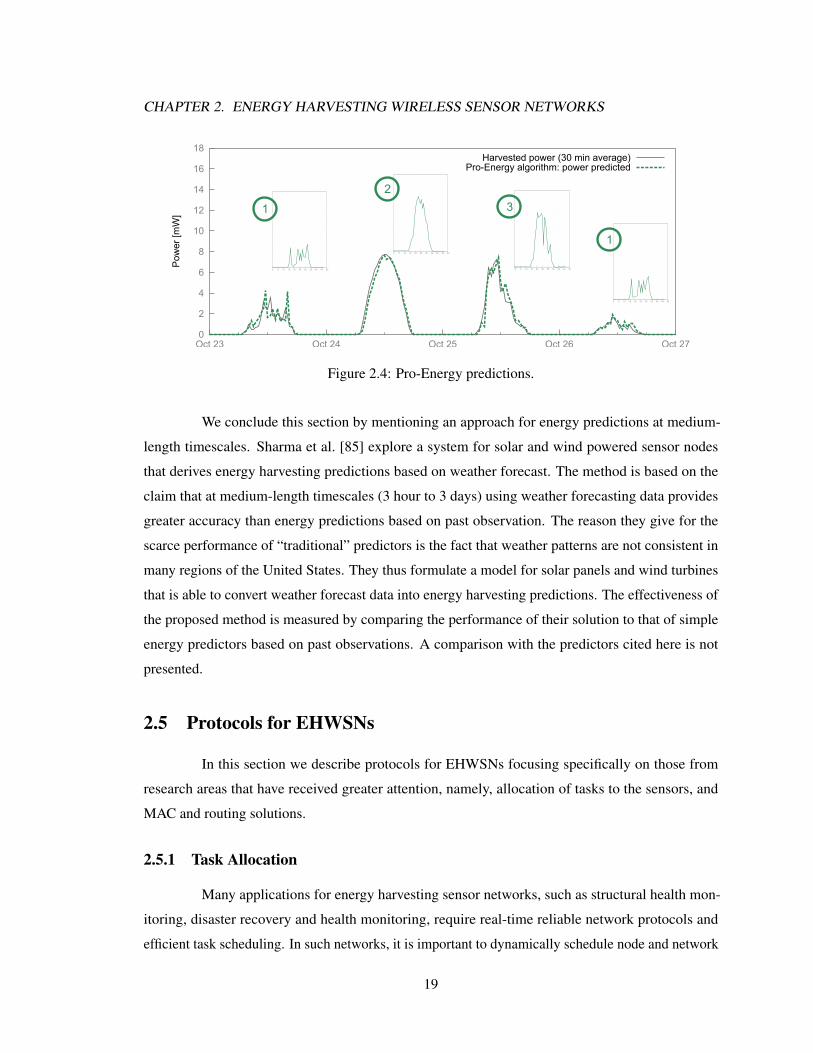
infrequently. Figure 2.4 shows an example of application of the Pro-Energy algorithm over 4 days
of solar predictions. During the initial time slots of October 23rd (day 1), the first stored profile is
selected among the typical ones, as it is the most similar to the portion of the current day observed so
far. As the day goes on, the shape of the profile changes according to the new observations. Two
further different profiles are used for predictions during days 2 and 3. Then, on the fourth day, the
first profile is selected again as the most similar to the current observations. Pro-Energy performance
compares favorably with respect to previous solutions. For instance, because of the use of energy
profiles of typical days, Pro-Energy is able to sensibly decrease prediction errors even in cases with a
variable mix of sunny and cloudy days, a case where EWMA instead exhibits poor performance.
18
CHAPTER 2. ENERGY HARVESTING WIRELESS SENSOR NETWORKS
0
2
4
6
8
10
12
14
16
18
Oct 23 Oct 24 Oct 25 Oct 26 Oct 27
Pow
er [m
W]
Harvested power (30 min average)Pro-Energy algorithm: power predicted
0 5 10 15 20 25 30 35 40 45 50
0 5 10 15 20 25 30 35 40 45 50
0 5 10 15 20 25 30 35 40 45 50
0 5 10 15 20 25 30 35 40 45 50
1
2
3
1
Figure 2.4: Pro-Energy predictions.
We conclude this section by mentioning an approach for energy predictions at medium-
length timescales. Sharma et al. [85] explore a system for solar and wind powered sensor nodes
that derives energy harvesting predictions based on weather forecast. The method is based on the
claim that at medium-length timescales (3 hour to 3 days) using weather forecasting data provides
greater accuracy than energy predictions based on past observation. The reason they give for the
scarce performance of “traditional” predictors is the fact that weather patterns are not consistent in
many regions of the United States. They thus formulate a model for solar panels and wind turbines
that is able to convert weather forecast data into energy harvesting predictions. The effectiveness of
the proposed method is measured by comparing the performance of their solution to that of simple
energy predictors based on past observations. A comparison with the predictors cited here is not
presented.
2.5 Protocols for EHWSNs
In this section we describe protocols for EHWSNs focusing specifically on those from
research areas that have received greater attention, namely, allocation of tasks to the sensors, and
MAC and routing solutions.
2.5.1 Task Allocation
Many applications for energy harvesting sensor networks, such as structural health mon-
itoring, disaster recovery and health monitoring, require real-time reliable network protocols and
efficient task scheduling. In such networks, it is important to dynamically schedule node and network
19

CHAPTER 2. ENERGY HARVESTING WIRELESS SENSOR NETWORKS
tasks based on remaining energy and current energy intake, as well as predictions about future energy
availability.
In this section, we first provide a classifications of tasks based on their type and character-
istics, and then we present an overview of task scheduling algorithms.
Tasks can be categorized as follows:
1. Periodic vs. Aperiodic. Depending on their arrival patterns over time, tasks are divided into
periodic and aperiodic. Periodic tasks arrive regularly and their inter-arrival time is fixed.
Aperiodic tasks, also called on-demand, have arbitrary arrival patterns.
2. Preemptive vs. Non-preemptive. A preemptive active task may be be preempted at any time,
while a non-preemptive task cannot be paused or stopped at any time during its execution.
3. Dependent vs. Independent. A task is defined to be independent if its execution does not
depend on the running or on the completion of other tasks. A dependent task cannot run until
some other tasks have completed their executions.
4. Multi-version tasks. Multi-version tasks have multiple versions, each with different character-
istics in terms of time, energy requirements and priority.
5. Node vs. Network tasks. Each EHWSN node can schedule two kind of tasks: Node and
network tasks. Tasks such as sensing, computing, and communication can be considered node
tasks. Examples of network tasks are routing, leader election, cooperative communication, etc.
Due to different characteristics of node and network tasks, they need different scheduling and
energy budgeting algorithms.
Each task is characterized by:
• Execution time. The amount of time during which a task is running on the CPU.
• Deadline: The time by which the task should be completed. If the task deadline passes before
completing the task, a deadline violation occurs.
• Power requirement: The amount of energy required by a task to be successfully completed.
This may include the energy necessary to perform sensing, computation, and communication
activities.
20

CHAPTER 2. ENERGY HARVESTING WIRELESS SENSOR NETWORKS
• Reward. Each task T may be associated with a value or reward r indicating its importance.
Rewards can be a function of a task priority [86, 87, 88, 89], invocation frequency [90],
utility [91], or any other metric. An instance of task i, Ti, contributes ri units to the total
system reward only if it completes by its deadline. The reward (priority) of each tasks may
change over time.
• Running speed: The speed of the task currently executing. Running speed can be adjusted by
employing Dynamic Voltage and Frequency Selection (DVFS) techniques, which lower the
operating frequency of the processor (CPU speed) and reduce its energy consumption [86]. As
the processor changes its operational frequency and voltage, the task execution speed varies
accordingly. Adjusting task speed is desirable because it allows a node to adapt the execution
speed of a task based on the energy source availability.
Task scheduling protocols for EHWSNs can be categorized depending on the type of tasks
they schedule. At the highest level, task scheduling solutions can be divided into protocols that
schedule node tasks and protocols that schedule network tasks.
Scheduling protocols for node tasks. The Lazy Scheduling algorithm (LSA) [92] is one of the
earliest work in EHWSN task scheduling. Tasks are dynamically scheduled depending on future
energy availability, the capacity of the energy storage, the residual energy, and the maximum power
consumption of the sensor node. In particular, LSA aims at keeping the energy storage level as high
as possible and starts executing a task T at time t only if the following conditions are met: T is ready
for execution; T has the earliest deadline among those of tasks that are ready; the sensor node will
not run out of energy if it executes T to completion (at its maximum power), and T will not miss its
deadline if the node starts executing it at time t. LSA introduces the concept of energy variability
characterization curve (EVCC), which captures the dynamics of the energy source. This concept
is used to determine the schedulability of a set of tasks. More specifically, the LSA uses an offline
schedulability test that, given the EVCC of the energy source, the capacity of the energy storage,
and the maximum power requirement of a running task, determines whether all the deadlines of
a given set of tasks can be met or not. LSA suffers several drawbacks. For instance, in realistic
application a task actual energy consumption does not depend on the worst case energy demand,
but rather on factors including the sensor operational state and the circuitry used to perform the
task. Furthermore, LSA does not consider dependency among tasks. Finally, the performance of
LSA is highly dependent on the accuracy of predicted available energy, which is challenging and, as
mentioned, prone to errors.
21

CHAPTER 2. ENERGY HARVESTING WIRELESS SENSOR NETWORKS
The STAM-STFU protocol by Audet et al. [93] combines the operation of two scheduling
algorithms, namely, Smooth to Average Method (STAM) and Smooth to Full Utilization (STFU),
for scheduling a set of tasks offline, with the aim of reducing the total task deadline violations.
STAM-STFU handles energy uncertainty and deadline constraints without relying on any energy
prediction model. STAM-STFU introduces the concept of virtual tasks to smooth out the energy
consumption in the long run. Each real (physical) task has a corresponding virtual task that has
the same arrival time, but equal or longer duration, and equal or smaller energy demand. Virtual
tasks are distributed over a longer execution time than their real counterparts, but each consumes the
same amount of energy as its corresponding real task. A scheduling for virtual tasks that meets the
deadline constraints will not violate the deadline of any real task. STAM-STFU smooths out real
task consumption to approximately the average power required by all tasks and then schedules them
by using the Earliest Deadline First algorithm. Simulation results show that STAM-STFU performs
better than non-energy-aware static scheduling algorithms. It is also shown that its performance is
similar to LSA that, with the additional benefit of not requiring a prediction model. It is important
to note that STAM-STFU is only suitable for offline scheduling, which requires that tasks and their
deadlines are known in advance.
The goal of the multi-version scheduling algorithm [90] is to execute the most important
and valuable periodic tasks while meeting all the timing and energy constraints. Each task is assumed
to have multiple versions, each with different characteristics and reward. “Easier” versions of
a task execute faster, require less energy, and produce less accurate and valuable results. This
static (offline) scheduling solution determines the best task versions and their execution speeds that
maximize rewards. Selection is based on worst case scenario assumptions, i.e., the worst-case task
execution times, worst-case number of speed changes, minimum harvesting rate, and worst-case
battery discharging rates, are assumed and known in advance. However, a system does not always
consume or harvest energy as in the worst-case, and often time the selection of tasks is not optimal.
To obviate to this problem, the authors propose dynamic algorithms according to which the node
periodically check the current energy storage and accordingly reschedule the tasks.
In [94] EL Ghor et al. describe an on-line scheduling algorithm, called EDeg (Earliest
Deadline with energy guarantee), a variant of the Earliest Deadline First algorithm. EDeg maintains
energy neutrality by making sure that before a task is started sufficient energy is in storage for all
future occurring tasks. This protocol assumes that future task arrival times are known. Task execution
is delayed until recharging has produced enough energy to meet the task deadline. When the stored
energy drops below a threshold EDeg stops the current tasks and starts recharging the battery up
22

CHAPTER 2. ENERGY HARVESTING WIRELESS SENSOR NETWORKS
to a level that support task completion. Thus, tasks never run in absence of enough energy. The
requirement to know in advance the arrival times, the deadlines, and the energy demands of the tasks,
seriously limits the applicability of this algorithm in real-life application scenarios.
Steck et al. [91] present a task utility scheduling protocol with two main goals: First, given
a certain level of utility, determine the expected execution time and energy consumption of a set
of tasks. Second, given a time constraint, find the maximum achievable utility for the set of tasks.
This algorithm schedules the tasks by balancing task utility and execution time subject to an energy
constraint aimed to ensure the energy neutrality of the system. The relationship among the tasks
is assumed to be known and modeled by a Directed Acyclic Graph (DAG). In addition, the task
execution times, past energy harvesting information, tasks qualities, and utility relationships are
given in advance. For most applications, the utility is modeled as accuracy and as a function of the
task priority. A task with higher priority is executed with the higher utility.
In [95], an energy-aware DVFS (EA-DVFS) scheduling algorithm is proposed that dynam-
ically matches its schedules to the stored energy and harvestable energy in the future. Specifically,
tasks are executed at full speed if the stored energy is sufficient. Execution speed is slowed down
when the stored energy is not sufficient. This work has been extended further in [87] by the adaptive
scheduling and DVFS algorithm (AS-DVFS). AS-DVFS adaptively tunes the operation voltage and
frequency of a node processor whenever possible while maintaining the time and energy constraints.
The goal of AS-DVFS is to reach a system-wide energy efficiency by scheduling and running the
tasks at the lowest possible speed and allocating the workload to the processor as evenly as possible.
Moreover, it decouples the timing and energy constraints, addressing them separately. A harvesting-
aware DVFS (HA-DVFS) algorithm is proposed in [86] to further improve the system performance
and energy efficiency of EA-DVFS and AS-DVFS. In particular, the main goals of HA-DVFS are to
keep the running speed of the tasks always at the lowest possible value and avoid wasting harvested
energy. Based on the prediction of the energy harvesting rate in the near future, HA-DVFS schedules
the tasks and tunes the speed and workload of the system to avoid energy overflow. Three different
time series prediction techniques, namely regression analysis, moving average, and exponential
smoothing, are used for predicting the harvested energy. Similar to AS-DVFS, HA-DVFS decouples
the energy constraints and timing constraints to reduce the complexity of scheduling algorithm.
Another DVFS-based task scheduling algorithm is presented in [88]. The basic DVFS
ideas are combined with a linear regression model. The model is used to associate the number of
tasks and their complexity to the execution time, energy consumption, and data accuracy. The main
objectives of this protocol are maximizing system performance given the current energy availability,
23

CHAPTER 2. ENERGY HARVESTING WIRELESS SENSOR NETWORKS
increasing the efficiency of energy utilization, and improving task accuracy. The protocol is deemed
specifically suitable for structural health monitoring applications, since the events generated by this
kind of applications concern mostly periodic tasks instead of sporadic externally triggered events.
Scheduling protocols for network tasks. Task allocation at the network level concerns matching
the sensing resources of a WSN to appropriate tasks (missions), which may come to the network
dynamically. This is a non trivial task, because a given node may offer support to different missions
with different levels of accuracy and fit (utility). Missions may vary in importance (profit) and amount
of resources they require (demand). They may also appear in the network at any time and may have
different duration. The goal of a sensor-missions assignment algorithm is to assign available nodes to
appropriate missions, maximizing the profit received by the network for mission execution. Although
solutions for WSNs with battery-operated nodes have been proposed for this problem [96, 97, 98, 99],
until recently [100] no attention has been given to networks whose nodes have energy harvesting
capabilities. For these networks, new paradigms for mission assignments are needed, which take into
account that nodes currently having little or no energy left might have enough in the future to carry
out new missions. These solutions should also consider that energy availability is time-dependent
and that energy storage is limited in size and time (due to leakage) so that energy usage should be
carefully planned to minimize waste of energy.
EN-MASSE [100] is a decentralized heuristic for sensor-mission assignment in energy-
harvesting wireless sensor networks, which effectively takes into account the characteristics of an
energy harvesting system to decide which node should be assigned to a particular mission at a
given time. It is able to handle hybrid storage systems consisting of multiple energy storage devices
(supercapacitor and battery) and to adapt its behavior according to the current and expected energy
availability of the node, while maximizing the efficient usage of the energy harvested. EN-MASSE
has been designed for sensing task assignment. Each mission arrives in the network at a specific
geographic location li. In EN-MASSE the sensor node closest to li is selected as the mission leader
and coordinates the process of assigning nodes to the mission. The communication protocol described
in [97, 98] is selected for exchanging information between the mission leader and the nearby nodes.
Each time a new mission arrives in the network, the leader advertises mission information, including
mission location, profit and demand, to its two-hop neighbors, starting the bidding phase for the
mission. During this bidding phase, each node receiving the mission advertisement message sent
by the leader, autonomously decides whether to bid for participating to the mission or not. Such a
decision is taken accordingly to the bidding scheme used by the node. EN-MASSE uses an energy
prediction model to estimate the energy a node will receive from the ambient source and to classify
24

CHAPTER 2. ENERGY HARVESTING WIRELESS SENSOR NETWORKS
missions. Different predictors, such as the ones described in Section 2.4, may be used in combination
with EN-MASSE.
2.5.2 Harvesting-aware Communication Protocols: MAC and Routing
Harvesting capabilities have changed the design objectives of communication protocols
for EHWSNs from energy conservation to opportunistic optimization of the use of the harvested
energy. This fundamental change calls for novel communication protocols. The aim of this section is
to explore the solutions proposed so far for EHWSN medium access control (MAC) and routing.
MAC protocols. We describe exemplary MAC protocols for EHWSNs, which include ODMAC [101],
EA-MAC [102, 103], MTTP [104], and PP-MAC [105].
ODMAC [101] is an on demand MAC protocol for EHWSNs. It is based on three basic
ideas: Minimizing wasting energy by moving the idle listening time from the receiver to the
transmitter; adapt the duty cycle of the node to operate in the energy neutral operation (ENO) state,
and reducing the end-to-end delay by employing an opportunistic forwarding scheme. In ODMAC,
transmission scheduling is accomplished by having available receivers broadcasting a beacon packet
periodically. Nodes wishing to transmit listen to the channel, waiting for a beacon. Upon receiving a
beacon, the transmitter attempts packet transmission to the source of the beacon. Setting the beacon
period imposes a trade-off between energy consumption and end-to-end latency: When the beacon
period is short, more energy is consumed for transmitting beacons. Longer beacon periods result in
higher energy conservation. Figure 2.5 shows the operation mechanism of the ODMAC protocol.
ODMAC supports a dynamic duty cycle mode, in which the sensing period and the beacon periods
of each node is periodically adjusted according to the current power harvesting rate. To this end, a
battery level threshold is selected and periodically compared the current battery level to determine if
the duty cycle should be increased or decreased. ODMAC also includes the concept of opportunistic
forwarding, in which, instead of waiting for a specific beacon, each frame is forwarded to the sender
of the first beacon received as long as it is included in a list of potential forwarders. In ODMAC it
is assumed that charging (harvesting) is independent of sensor node operations and thus a sensor
can harvest available energy during all operational states, i.e., irrespective of whether it is sleeping,
listening, transmitting, etc. ODMAC is not suitable to be used in lossy environment, as it does not
acknowledge and retransmits packets.
EA-MAC [102, 103] is a MAC protocol proposed for EHWSNs with RF energy transfer.
EA-MAC uses the node energy harvesting status as a control variable to tune the node duty cycles and
25

CHAPTER 2. ENERGY HARVESTING WIRELESS SENSOR NETWORKS
back-off
T_IFS Listen
(T<=T_tx)
Source
Beacon
Listen
(T<=T_tx)
Sensing / Wait for Beacon
Beacon
Listen
DataReceive
Beacon
Sleeping
Sleeping
Listen for DataListen for
DataReceive Data Beacon
Sleeping
T_IFS T_IFS
DestinationSleeping
Figure 2.5: ODMAC: data packet transmission.
back-off times. To this end, two adaptive methods, energy adaptive duty cycle and energy adaptive
contention algorithm, are proposed to manage the node duty cycle and back-off time depending
on the harvested power rate. EA-MAC is similar to the unslotted CSMA/CA algorithm in IEEE
802.15.4 [106], but its sleep duration, back-off times, and state transitions are controlled by the
average amount of harvestable energy. When a node harvested energy level is equal to the energy
required to transmit a packet, the node transitions from sleep state to active state. Then it follows a
CSMA/CA scheme to transmit the packet. If the channel is idle during the clear channel assessment
(CCA) period, the node transmits a data packet. If the channel is busy, the node decides to either
perform the random backoff procedure or terminate the CSMA/CA algorithm. The number of
backoff slots depends on the current energy harvesting rate. Analytical models for the throughput and
fairness of EA-MAC are provided and validated by simulations [103]. Similar to ODMAC, EA-MAC
assumes the sensor node can harvest energy in any operational states. EA-MAC does not consider
some important application requirements, such as end-to-end delay, and provides no mechanism to
optimize network performance and lifetime. In addition, EA-MAC suffers form the hidden terminal
problem, which results in increased collisions. Finally, its performance is not compared to any other
protocol, such as slotted or unslotted CSMA/CA.
The Probabilistic polling (PP-MAC) protocol [105] is a polling-based MAC mechanism
that leverages the energy characteristics of EHWSNs to enhance the performance of traditional
polling schemes in terms of throughput, fairness and scalability. PP-MAC is similar to the polling
protocol described in [107]: The sink broadcasts a polling packet and the polled sensor responds
26

CHAPTER 2. ENERGY HARVESTING WIRELESS SENSOR NETWORKS
Tire 1
Sensors
Sink
Tire 2
Sensors
Polling
PacketPolling
Packet
Polling
Packet
Data
Data
Polling
Packet
Figure 2.6: Overview of MTTP multi-tier EHWSN architecture.
with a packet transmission (single-hop topology). Instead of carrying the ID of a specific sensor,
the polling packet contains a contention probability that the receiving sensor nodes use to decide
whether to transmit their packet or not. The contention probability is computed based on current
energy harvesting rate, number of nodes, and packet collisions. The probabilistic polling protocol
increases the contention probability gradually when no sensor responds to the polling packet. It
decreases it whenever there is a collision between two or more sensor nodes. As a result, and based
on an additive-increase multiplicative-decrease (AIMD) mechanism, the contention probability is
decreased when more nodes are added to the EHWSN, and increased when nodes fail or are removed
from the network. Moreover, in case of increase/decrease of the average energy harvesting rates,
the contention probability is decreased/increased accordingly. PP-MAC uses the charge-and-spend
harvesting strategy in which it first accumulates enough energy and then goes to the receive state to
listen and receive the polling packet. Nodes return back to charging state either when their energy
falls below the energy required to transmit a data packet or after transmitting their packet. Energy
is assumed to be harvested only while in charging state. Analytical formulas and analysis of the
throughput performance of PP-MAC is presented and validated by simulations. PP-MAC does not
support multi-hop EHWSNs.
The multi-tier probabilistic polling (MTPP) protocol [104] extends probabilistic polling a
la PP-MAC to multi-hop data delivery in EHWSNs with no energy storage, i.e., whose operations
are powered solely by energy currently harvested (charge-and-spend harvesting policy). The polling
packets generated by the sink are sent to the immediate neighbors of the sink, and these nodes forward
them to nodes in following tiers, in a “wave-expanding” fashion (Figure 2.6). Polling packets and
27

CHAPTER 2. ENERGY HARVESTING WIRELESS SENSOR NETWORKS
data packets are broadcast and relayed, respectively, from tier to tier until they reach their destination.
As the number of tiers increases, the overhead of polling packets and packet collisions also increase,
imposing higher latencies. Analytical models for energy consumption, energy harvesting, energy
storage, and interference as well as the delivery probability are presented in [108] and validated by
numerical analysis.
A comparative summary of the characteristics of these presented MAC protocol is presented
in Table 2.1.
ODMAC EA-MAC PP-MAC MTTP
Topology Multi-hop Single-hop Single-hop Multi-hop
Harvesting policy Store Store Charge-and-spend Charge-and-spend
Harvesting technology Generic RF energy transfer Solar Solar
Latency Increases with traffic Fair Low High
Channel access type CSMA/CA CSMA/CA Polling Polling
Scalability Good Weak Good Good
Communication patterns All Convergecast Convergecast Convergecast & Broadcast
Performance evaluation OPNET simulations OPNET simulations Real-measurements & QualNet Real-testbed
Use of control packets Yes No Yes Yes
Adaptivity to changes Fair Good Good Good
Table 2.1: Comparison of MAC protocols for EHWSNs.
Routing protocols. Energy-efficient routing has been widely explored for battery operated WSNs.
EHWSNs exhibit unique characteristics and among their man objective there is not only extending
the network lifetime, but also the maximization of the workload that the network can sustain, given
the source-dependent energy availability of the nodes [109]. This is the rationale behind protocols
for routing in EHWSNs that we present in this section.
HESS. In [110], Pais et al. propose a routing protocol termed HESS for hybrid energy
storage systems combining a supercapacitor with a rechargeable battery. Their approach is to favor
routes that use more energy from supercapacitors and that go through nodes with higher harvesting
rates. Their work stems from the fact that a rechargeable battery can only sustain a limited amount of
recharge cycles before its capacity falls below 80% of its original capacity. The authors propose a
cost-benefit function that reflects the cost and revenue of choosing a specific node as a relay for a
packet. Such a function considers several factors, including the relay hop count, its residual battery
and supercapacitor energy, the energy it harvested previously, the remaining cycles of its battery and
its queue occupancy. Nodes with higher residual energy, harvesting rate and remaining battery cycles
are preferred as relays, while choosing nodes with higher hop count or lower transmission queue
28

CHAPTER 2. ENERGY HARVESTING WIRELESS SENSOR NETWORKS
availability is less desirable. These cost/benefit factors are combined together, opportunely weighted,
in order to account for both desirable and undesirable parameters. The overall goal of HESS is to
minimize the cost of each end-to-end transmission. A simulation-based performance evaluation
shows that HESS provides an average 10% increase of network residual energy with respect to the
Energy Aware Routing (EAR) protocol [111], without compromising the data packet delivery ratio.
DEHAR (Distributed Energy Harvesting Aware Routing Algorithm, Jakobsen et al. [112])
is an adaptive and distributed routing for EHWSNs that calculates the shortest paths to the sink based
on hop count and the energy availability of the nodes. To add energy-harvesting awareness to the
algorithm, a local penalty is assigned to each node. This penalty, dynamically updated, is inversely
proportional to the fraction of energy available to the node. When the energy buffer of the node is
fully charged, this penalty should ideally be zero, while it should tend to infinity when the node
has depleted its energy. When a change in the local penalty of a node occurs, it advertises it to its
immediate neighbors. For each node, the local penalty is combined with distance from the sink
to define the node energy distance, which is used by other nodes when choosing a potential relay.
The energy distance of a node may become a local minimum if the penalty of a node neighbor is
changed due to variations in its energy availability. To solve this problem, distributed penalties are
introduced. Each time a node receives an energy update from a neighbor, it checks if it has become a
local minimum. If this is the case, it increases its distributed distance penalty and advertises it to its
immediate neighbors. Distributed and local penalty of a node are finally merged in a total penalty
that is distributed to neighbor nodes.
EHOR: Energy Harvesting Opportunistic Routing (Eu et al. [113]) is an opportunistic
routing protocol for EHWSNs powered solely by energy harvesters (no batteries). Nodes of EHWSNs
powered only by harvested energy are normally awake for a short period of time, then they shut
down to recharge. To determine the best active relays in its neighborhood, a node partitions potential
relays in groups, or regions, based on their distance from the sink and on the residual energy of the
nodes in the region. After receiving a data packet, the potential relay that is the closest to the sink
rebroadcasts it. Each node in the network follows a charging cycle consisting of a charging phase,
during which the power consumption is minimal and the node waits to be recharged by the harvested
energy, a receive phase, to which the node switch when it is fully charged, and an optional transmit
phase. Simulation results show that EHOR achieves good performance and outperforms traditional
opportunistic routing protocols. EHOR, however, assumes that the network topology is linear, i.e.,
that nodes are uniformly deployed over a given interval and does not work in 2D topologies.
Noh and Yoon introduce D-APOLLO (Duty cycle-based Adaptive toPOLogical KR aLgO-
29

CHAPTER 2. ENERGY HARVESTING WIRELESS SENSOR NETWORKS
rithm [114]) a harvesting-aware geographic routing protocol. Their approach aims at maximizing
the utilization of the harvested energy and reduce latency by dynamically and periodically adapt
the duty-cycle and the knowledge range (KR) of each node. The knowledge range of each node is
the topological extent of the information that it collects. Dimensioning the KR involves a trade-off
between the optimality of the path produced by the routing algorithm and the energy needed to
collect and maintain a larger quantity of information about a node neighbors. The duty cycle of the
nodes and their knowledge range are usually fixed in battery-operated WSNs. D-APOLLO, instead,
periodically tries to find the duty cycle and the knowledge range that maximize utilization of the
harvested energy based on the expected harvesting power rate, the residual energy of the node and
the predicted energy consumption.
The Energy-opportunistic Weighted Minimum Energy (E-WME, Lin et al. [115]) calculates
the shortest path to the sink based on a cost function metric that considers the residual energy of
the node, its battery capacity, it harvesting power rate and the energy required for receiving and
transmitting packets. The cost of each node is an exponential function of the nodal residual energy, a
linear function of the transmit and receive energies, and an inversely linear function of the harvesting
power rate. The authors show that as an online protocol E-WME has an asymptotically optimal
competitive ratio and that it can lead in practice to significant improvements in the performance of
EHWSNs with respect to other harvesting-unaware routing protocols.
Bogliolo et al. present a modified version of the Ford-Fulkerson algorithm to determine the
maximum energetically-sustainable workload of an EHWSN [116]. Their Randomized Max-Flow
(R-MF) protocol, and its enhancement Randomized Minimum Path Recovery Time (R-MPRT) [109],
select the edge over which to route the packet with probability proportional to the maximum flow
through that edge. More specifically, in R-MF and R-MPRT the cost Cu,v of routing a packet through
a link (u, v) is expressed as
Cu,v =pu
eu,vrouting, (2.1)
where pu is the harvesting power rate of node u, and eu,vrouting is the energy needed to process or
generate a packet at node u and to transmit it to node v through the link (u, v).
Hasenfratz et al. analyze and compare three state-of-the-art routing protocols for EHWSNs:
R-MF, E-WME and R-MPRT [117]. In their work, they show the influence of various real-life
settings on their performance, namely, 1) the usage of a low-power MAC protocol instead of an
ideal one; 2) the effect of considering a realistic wireless channel, and 3) the influence of the
30

CHAPTER 2. ENERGY HARVESTING WIRELESS SENSOR NETWORKS
protocol overhead. They also propose a modified version of the R-MPRT algorithm, which is able
to outperform R-MPRT in scenarios where little energy is harvested from the environment. More
precisely, they suggest to modify Equation (2.1) as follows:
Cu,v =Eu
eu,vrouting, (2.2)
where Eu is the amount of energy available at node u, and eu,vrouting is the energy needed to process
or generate a packet at node u and transmit it to node v through the link (u, v).
In [118], Zeng et al. propose two geographic routing algorithms, called GREES-L and
GREES-M, which take into account energy harvesting conditions and link quality. Each node is
required to maintain its one-hop neighbor information including the neighbors location, residual
energy, energy harvesting rate, energy consuming rate, and wireless link quality. While forwarding
a packet towards its destination, the nodes in the network try to balance the energy consumption
across their neighbors, by minimizing a cost function combining the information they maintain.
Such cost function is defined based on two factors, namely, the geographical advance per packet
transmission and the energy availability of the receiving node. The difference between GREES-L
and GREES-M is in the way they combine the two factors: GREES-L uses a linear combination
of them, while GREES-M multiplies them. GREES-L and GREES-M only consider as potential
relay neighbor nodes that provide positive advancement towards the sink, which is typical of greedy
geographic forwarding. GREES-L and GREES-M have been shown to be more energy efficient than
the corresponding residual-energy-based protocols via simulations.
There are two important quality metrics to take into account while comparing energy
harvesting techniques. First is the power density and the second is conversion efficiency. The
power density is the rate of harvested energy per unit volume, area, or mass. The common metrics
of power density include: watts per square centimeter and watts per cubic centimeter. The other
important property of energy harvesting is the conversion efficiency, which is defined as the ratio of
the harvested electrical power to the harvestable input power. Note that energy conversion efficiency
is a dimensionless number between 0 to 100%. Table 2.2. compares the power density and conversion
efficiency of different energy harvesting techniques.
2.6 Final Remarks
This chapter covers the fundamental aspects of EHWSNs, ranging from the architecture
of a EHWSN node and of its energy subsystem to protocols for task allocation, MAC and rout-
31

CHAPTER 2. ENERGY HARVESTING WIRELESS SENSOR NETWORKS
Energy harvesting technique Power density Efficiency
Photovoltaic Outdoors(direct sun): 15 mW/cm2 Highest: 32± 1.5%
Outdoors(cloudy day): 0.15 mW/cm2 Typical: 25± 1.5% [119]
Indoors: <10 µW/cm2 [120, 36, 37, 50]
Thermoelectric Human: 30 µW/cm2 ±0.1%
Industrial: 1− 10 mW/cm2 [121, 50] ±3% [50]
Pyroelectric 8.64 µW/cm2 at temperature rate 8.5C/s [122] 3.5% [123]
Piezoelectric 250 µW/cm3 a
330 µW/cm3 (shoe inserts) [36, 37]
Electromagnetic Human motion: 1− 4 µW/cm3[124, 68] a
Industrial: 306 µW/cm3 [125], 800 µW/cm3 [68]
Electrostatic 50− 100 µW/cm3 [34] a
RF GSM 900/1800 MHz: 0.1 µW/cm2 50% b[126]
WiFi 2.4 GHz: 0.01 µW/cm2 [120]
Wind 380 µW/cm3 at speed 5 m/s [40, 127] 5% [40]
Acoustic Noise 0.96 µW/cm3 at 100 dB c
0.003 µW/cm3 at 75 dB [128, 16]
a Max power and the efficiency are source dependent.b Excluding the transmission efficiency.c Noise power densities are theoretical values.
Table 2.2: Comparison of power density and efficiency of different energy harvesting techniques
ing, passing through models for predicting energy availability. With the advancement on energy
harvesting techniques, and the development of small factor harvester for many different energy
sources, EHWSNs are poised to become the technology of choice for the host of applications that
require network functionalities for years or even decades. Through the definition of new hardware
and communication protocols specifically tailored to the fundamentally different models of energy
availability, new applications can also be conceived that rely on “perennial” functionalities from
networks that are truly self-sustaining and with low environmental impact.
32

Chapter 3
Reliability Modeling of Energy
Harvesting Sensor Nodes
3.1 Introduction
Energy harvesting wireless sensor networks (EHWSNs) are made up of wireless sensor
nodes powered by rechargeable batteries that are replenished through energy scavenged from re-
newable or ambient sources. Such a charging paradigm extends the network lifetime by reducing
the charge drawn from the battery, prevents disruptions owing to battery replacement, and ensures
environmentally friendly operation. However, as the residual energy at the node is time varying, and
is subject to a variety of other factors, it is a challenge for the network designer to formulate closed
form expressions that indicate future energy levels and lifetime of a EHWSN node. The analytical
framework proposed in this chapter, called Stochastic Analysis and aVailability of Energy (SAVE),
takes the first step towards this direction.
Recent research on analyzing the lifetime and energy consumption in “classical,” battery-
limited WSNs has been presented in [129, 130, 131] (average analysis) and [132, 133] (distribution
analysis). However, the key consideration of re-charging the energy reserve is not considered in
these works. Seyedi et al. present a Markov-based model for energy harvesting nodes in a body
sensor network [134]. The work provides an an analysis of the probability of event loss due to energy
depletion. Moreover, Ventura and Chowdhury present MAKERS, a Markov based model for one or
multiple-sources energy harvesting nodes in WSNs [135]. This work provides analytical model for
predicting the probability of a sensor running out of energy with very low computational complexity.
33

CHAPTER 3. RELIABILITY MODELING OF ENERGY HARVESTING SENSOR NODES
In addition, it can model energy harvesting sensors equipped with multiple energy harvesting boards.
Sus et al. present DTMC for environmentally powered sensor nodes for assessing statistical properties
such as the probability of achieving a given operation time and the expected downtime [136]. While
re-charging is considered, these models are examples of average analysis, where only the long term,
average behavior of the nodes is ascertained, and do not consider the stochastic nature of energy
availability.
SAVE is a general analytical framework that provides a stochastic tool for the analysis of
the residual energy and the lifetime distribution of EHWSN nodes. We model the energy harvesting
wireless sensor node (harvesting node, from now on) as a stochastic semi-Markov process and
introduce a new analysis technique, called energy transient analysis, for the computation of the net
consumed energy distribution. The amount of consumed and harvested energy in each state of a
node are modeled as random variables, depending on discharging and recharging rates and on the
holding time distribution of that state. The main contributions of this chapter include the following:
(i) We introduce SAVE for node residual energy and lifetime predictions at any time, based on the
distributions of harvested energy, net-consumed energy (by processing, wireless re/transmissions,
and sleep-awake cycles), and node lifetime. (ii) We show that SAVE is not limited to exponential or
fixed holding time distributions in each Markov state. The operational states can have general and
arbitrary holding time distributions, resulting in a more accurate and flexible analytical framework.
(iii) We present a new technique called energy transient analysis serving as a tool for deriving the
energy distributions based on the semi-Markov process of a harvesting node. This technique is
harvesting technology- and harvesting node-independent, thus being applicable in a wide variety of
practical settings.
3.2 The SAVE Analytical Framework
We consider nodes equipped with one or multiple energy harvesting modules, working
under different energy sources, each with their independent charging and discharging rates. SAVE
models a harvesting sensor node as a semi-Markov process (SMP) in which each state corresponds to
a node operational mode. A SMP is a type of stochastic process whose states change as in a Markov
chain, but where the permanence in a particular state happens for a random amount of the time (called
holding time), following a given distribution. The holding time depends on the current state and on
the next state to be visited. In a SMP, each state is associated with one or more reward variables
called reward rates. In the case of SAVE, every state i has two reward rates: Power discharging
34

CHAPTER 3. RELIABILITY MODELING OF ENERGY HARVESTING SENSOR NODES
(battery consumption) rate di and power recharging (energy replenishment) rate ri. The discharging
rate depends on the node hardware specifications and on the node operation of that state. The power
recharging rate depends on the renewable energy source.
With Xh = X(t) : t ≥ 0 we represents the SMP of the harvesting node h with
sample states S = 1, 2, ..,M, M being the number of a harvesting node operational states. The
random variable X(t) indicates the state of the system at time t. The Markov renewal process
Z = (Zn, Tn);n ≥ 0 is connected to the SMP Xh as follows:
X(t) = Zn, Tn ≤ t < Tn+1,
where n is the number of state transitions that has taken place by time t, Zn ∈ S is the state after
the nth transition and Tn is the time of the nth transition. The state transition probability Pij , which
governs the change from state i to state j, is defined as follows:
Pij = PrX(T1) = j|X(0) = i.
Accordingly, P = [pij ] is the transition probability matrix. The kernel of the semi-Markov
process is independent of the number n ≥ 0 of transitions, and it is defined as:
K(i, j, t) = Pr(Zn+1 = j, Tn+1 − Tn ≤ t|Zn = i),
or, equivalently:
K(i, j, t) = PijQij(t).
In the latter equationQij(t) denotes the holding time distribution of state i, after a transition
from state i to state j has occurred. More specifically:
Qij(t) = Pr(Tn+1 − Tn ≤ t|Zn+1 = j, Zn = i).
The state transition probabilities and holding time distributions depend on the specific
network and protocol parameters.
The matrix K(t) = [K(i, j, t)] is the kernel matrix of the harvesting node and stores
information on the harvesting node operations. This is the information we need for computing the
energy and node lifetime distributions. In other words, the stochastic nature of the harvesting node
is captured by the kernel of its SMP. The distribution of the holding time in a particular state i is
obtained from the kernel matrix of the SMP as follows:
35

CHAPTER 3. RELIABILITY MODELING OF ENERGY HARVESTING SENSOR NODES
Qi(t) =∑j∈S
K(i, j, t).
Fig. 3.1 shows two generic states of the SMP representing a harvesting node. The time-
varying behavior of a harvesting node from state i to state j is expressed by the transition probability
Pij and the holding time distribution Qij(t), while the power discharging and recharging rates
capturing the consumed and harvested energies.
power discharging rate:
Operationalstate i
Operationalstate j
ijP
P Qji
(t)Q
(t)
ij
ji
djr j
,
,di
power recharging rate: ri
Figure 3.1: A harvesting node as a semi-Markov process.
3.2.1 Residual Energy Distribution
The amount of residual energy at a harvesting nodes over time plays a key role in funda-
mental network functions, such as its connectivity, coverage and lifetime. In this section, we derive
the distribution of the energy available at a harvesting node at a given time T .
The amount of energy consumed in state i is a random variable Ei that depends on the
discharging rate di and on the probability distribution of the holding time in that state. Similarly, the
amount of harvested energy in state i is a random variable Hi that depends on the recharging rate ri
and the holding time distribution. The energy consumption distribution in state i when a transition
from state i to state j occurs, is as follows:
Eij(e) = Pr(Ei ≤ e|Zn+1 = j, Zn = i).
For example, if the discharging rate in state i is di andQij(t) is the holding time distribution
before the harvesting node moves into state j, the energy consumption distribution Eij(e) is:
Eij(e) = Qij(e
di).
36

CHAPTER 3. RELIABILITY MODELING OF ENERGY HARVESTING SENSOR NODES
Similarly, the energy harvesting distribution in state i when SMP moved from state i to j
is:
Hij(e) = Pr(Hi ≤ e|Zn+1 = j, Zn = i).
The unconditional energy consumption and harvesting distributions in state i when a
transitions form state i to state j occurs are:
E(i, j, e) = Pr(Zn+1 = j, Ei ≤ e|Zn = i) = PijEij(e)
and:
H(i, j, e) = Pr(Zn+1 = j,Hi ≤ e|Zn = i) = PijHij(e),
Clearly, considering the discharging and recharging rates, both of the two last distributions
could be computed based on the kernel of the semi-Markov process. The distribution of energy
consumption and harvesting in state i are finally obtained as follows:
E(i, e) =∑j∈S
E(i, j, e) and H(i, e) =∑j∈S
H(i, j, e).
We now describe a new energy transient analysis technique for computing the distributions
of the consumed and of the harvested energy. We assume that the harvesting node starts in state i
and after time T is in state k. Throughout time T the node might have transitioned through different
sequences of states (paths in the SMP). However, independently of the followed path, for each state
m in the path the harvesting node consumes a random amount of energy Em and harvests a random
amount of energy Hm. Both random values Em and Hm depend on the state holding time probability
distribution, and on the discharging and recharging rates associated to state m. Therefore, the total
amount of energy consumed and harvested over a path of N states from state i to state k during time
T can be obtained as the sum of N independent random variables:
Eik(T ) = Ei + Ei+1 + . . .+ Em + . . .+ Ek, and
Hik(T ) = Hi +Hi+1 + . . .+Hm + . . .+Hk,
where k = N + i− 1. The probability density function (pdf) feik(e, T ) of Eik is defined such that:
Pr(e1 ≤ Eik ≤ e2) =
∫ e2
e1
feik(e, T ).
37

CHAPTER 3. RELIABILITY MODELING OF ENERGY HARVESTING SENSOR NODES
The pdf fhik(e, T ) of Hik is defined similarly. Recall that the pdf of the sum of N indepen-
dent random variables is the N -fold convolution of their pdfs. Therefore, in order to determine the
joint conditional pdf of energy consumption (conditioned with respect to time T and initial state i) it
is necessary to convolve the energy consumption pdfs of the states, dEij(e)de , over all possible paths
starting from state i and finishing in state k throughout time T . To this end, we calculate the Laplace
transform of the convolutions over all possible paths with different state holding times. This is done
through the following theorem.
Theorem 1 For any given time T , the Laplace transform Leik(s, T ) of feik(e, T ) with respect to e, is
the solution of the following equation:
Leik(s, T ) = e−sdiT (1− E(i, diT ))
+∑m
∫ Tdi
0e−seLemk(s, T −
e
di)dE(i,m, e),
where m ranges over all states in the SMP X , and di is the discharging rate in state i.
Proof 1 Let E be a random variable with cumulative distribution function (CDF) F(e). The Laplace-
Stieltjes transform (LST) of F is defined as follows:
E(e−sE ;E ≤ e|Z0 = i) =
∫ ∞0
e−sedF (e).
The Laplace transform of feik(e, T ) is as follows:
Leik(s, T ) = E(e−sEik(T );Eik(T ) ≤ e|Z0 = i),
where the random variable Eik(T ) shows the total amount of consumed energy during
time T starting from state i. Conditioning on the initial state energy consumption Ei we have:
E(e−sEik(T );Eik(T ) ≤ e|Ei = c, Z0 = i) =e−sdiT c ≥ diT ,
e−sc∑
m Lemk(s, T −
cdi
) c < diT .
Now, unconditioning with respect to Ei, we obtain:
38

CHAPTER 3. RELIABILITY MODELING OF ENERGY HARVESTING SENSOR NODES
Leik(s, T ) =∫ Tdi
0e−se
∑m
Lemk(s, T −e
di)dE(i,m, e)
+e−sdiT (1− E(i, diT )) =∑m
∫ Tdi
0e−seLemk(s, T −
e
di)dE(i,m, e)
+e−sdiT (1− E(i, diT )).
Similarly, Lhik(s, T ) is calculated as follows:
Lhik(s, T ) =∑m
∫ Tri
0e−seLhmk(s, T −
e
ri)dH(i,m, e)
+e−sriT (1−H(i, riT )),
where ri is the recharging rate in state i. The energy available at the harvesting node at time
T is defined as the residual battery energy taking into account the net consumed energy until time T .
The net consumed energy includes both consumed and harvested energies. Since the consumption
process is stochastically independent of the harvesting process, we can derive the Laplace transform
of the net consumed energy during time T as
Li(s, T ) = Leik(s, T )Lhik(s, T ),
Thus, the pdf f(e, T ) of the net consumed energy e consumed through time T can be
calculated by numerically inverting the Laplace transform Li(s, T ). Then, the CDF E(e, T ) is found
by∫ e
0 f(e, T )de. Note that such distribution depends on the initial state i, which in this work is
assumed to be always the sleep state. Finally, the distribution of the energy available to harvesting
node, residual energy, after time T is given by:
PA(e, T ) = E(E0 − e, T ). (3.1)
which depends on the overall net consumed energy distribution E(e, T ) and the initial
energy of the primary battery E0. The set of transitions from one specific state (e.g., sleep state) to
the next visit to that state construct a harvesting node operational cycle. As a special case, the energy
39

CHAPTER 3. RELIABILITY MODELING OF ENERGY HARVESTING SENSOR NODES
distributions regarding the number of cycles can be found based on the steady-state probabilities
of the SMP, πi, and the average time spent in each state, µj . In particular, the average length of
one cycle is equal to∑
j πjµj , and accordingly one can compute the Laplace transform of the net
consumed energy and its equivalence residual energy for different number of cycles.
3.2.2 Node Lifetime Distribution
In this section, considering the sensor semi-Markov model X(t), we characterize the
harvesting node lifetime distribution as a function of time (or number of cycles). Let g be the power
consumption reward function which for any time t over the operation of the sensor defined as:
g(X(t)) = di ≥ 0, if X(t) = i,
where g(X(t)) indicates the power consumption per unit time in the state i (at time t). Similarly, we
consider f to be the charging reward function as:
f(X(t)) = ri ≥ 0, if X(t) = i,
ri represents the energy recharging rate of the harvesting sensor in state i. We define the net consumed
energy E(t) as a random variable which takes into consideration both accumulated charging and
discharging energies of a harvesting sensor node in time as follows:
E(t) =
∫ t
0[g(X(τ))− f(X(τ))]dτ
=
∫ t
0[dX(τ) − rX(τ)]dτ =
∫ t
0eX(τ)dτ.
where ei indicates the combined reward rate in state i whenX(t) = i and E(t) is a stochastic process
based on X(τ) for 0 < τ < t. The harvesting sensor node lifetime can be defined as a random
variable T representing the time to accumulate a combined reward requirement equal to a random
variable w which represents the initial energy of the sensor’s battery (w = E0) :
T (w) = mint ≥ 0 : E(t) = w,
Moreover, node lifetime T is the time instant at which the overall (net) consumed energy by the
sensor node reaches the value w for the first time. Given that the initial state is i, the probability that
harvesting node consumes more accumulated energy than w during sensor operation time t is :
Pr(E(t) > w|X(0) = i),
40

CHAPTER 3. RELIABILITY MODELING OF ENERGY HARVESTING SENSOR NODES
Table 3.1: Parameters of SAVE Framework for the case study
Parameter Meaning
E0 Initial energy of the on-board battery
G Maximum number of retransmissions
BER Channel bit error rate
Pe Packet error rate
PB Channel busy probability
K Maximum number of backoff occurrences
Ts Sleeping period
Tw Wakeup period
λe Average event arrival rate
Sp Data packet size
SM Data message size
SH Packet header size
Rtx Channel transmission rate
tch Average charging time
Psc Charging probability
B Average processing time per event
PI Event of interest probability
which is exactly the probability that the lifetime of the harvesting node is shorter than t. Correspond-
ingly, the conditional node lifetime distribution which is the probability distribution that the sensor
node achieves the desired lifetime t, when i is the given initial state, would be as :
Pr(T (w) ≤ t|X(0) = i) = Pr(E(t) > E0|X(0) = i),
3.3 Framework Analysis: A Case Study
In section II, we described a general analysis framework for any arbitrary state diagram
that defined the operation of an energy harvesting sensor. In this section, we take a specific example
of a sleep-awake duty cycled sensor that harvests energy with an exponential charging time, and uses
a CSMA-based MAC protocol with ARQ for error recovery at the link layer. A detailed description
of the variables used is given in Table I.
41

CHAPTER 3. RELIABILITY MODELING OF ENERGY HARVESTING SENSOR NODES
Sleeping(S)
Charging(C)
Listening(L)
Processing(P)
Transmitting(T)
P sc
Pcl
Plp
Ppt
Pts
Psl
Pls
Pps
Figure 3.2: Semi-Markov Chain of a harvesting sensor node
3.3.1 Semi-Markov Chain Overview
The functions of the harvesting sensor node is modeled as a semi-Markov chain consisting
of (i) charging (C), (ii) sleeping (S), (iii) listening (L), (iv) processing (P), and (v) transmitting (T)
operational states, which are represented in Fig. 3.2 with their corresponding abbreviations in the
parenthesis. The operation of the sensor for this example scenario is described in the following,
assuming the above states:
3.3.1.1 Energy Harvesting Policy
The initial energy of the primary battery is E0. During its reduced activity sleep time (i.e.,
in state S), the sensor may either transition into deep sleep and charge (i.e., enter state C) with the
probability Psc, which is equal to a given charging probability, for an exponentially distributed time
with the mean value of tch, or continue in its current state with probability 1−Psc for a fixed sleeping
period Ts. Note that while our framework supports any arbitrary harvesting policy, for the purpose of
tractability, we assume here an exponential charging time. After completing the sleeping period Ts,
the node switches to the listening state (i.e., state L) and starts sensing the environment.
3.3.1.2 Event Processing
The node returns back to the sleeping state when no event is detected, or else it processes
the detected events in the processing state (i.e., state P) to find out if any of them are the events of
interest. The processing time per event follows an exponential distribution with mean B, though our
42

CHAPTER 3. RELIABILITY MODELING OF ENERGY HARVESTING SENSOR NODES
general model supports arbitrary distributions. Consequently, the processing time of R events has
R-stage Erlang distribution.
3.3.1.3 MAC Protocol
After completion of the processing stage, if any desired event is detected, the node switches
to the transmitting state (i.e., state T) with probability Ppt, which is derived later in Section III-B. If
the sensor node finds the channel idle during its initial carrier sensing, it begins transmitting. But if
the channel is busy with probability PB , the node defers its transmission for a random amount of
time. It waits in the idle mode, and probes the wireless channel again after that time. A maximum
number of K backoff occurrences for each packet is assumed. Moreover, the path loss wireless
channel is modeled with a two-state discrete Markov chain known as Gilbert model in which Pe
indicates the average packet error probability and is computed based on the wireless channel bit error
rate. Finally, an ARQ error control mechanism with G maximum number of packet retransmissions
is considered.
3.3.2 Constructing the SMP Kernel
In this section, we construct the kernel matrix of our example. In particular, each kernel
has two elements: probability transition matrix (P) and holding time distribution matrix (Q). Next, we
derive the transition probabilities and holding time distributions of our SMP described in Figure 3.2.
Note that the matrix elements for non-existent transition paths in SMP are zero.
P =
Pss Psc Psl · · · Pst
Pcs Pcc Pcl · · · Pct...
......
. . ....
Pps Ppc Ppl · · · Ppt
Pts Ptc Ptl · · · Pts
Q =
Qss(t) Qsc(t) Qsl(t) · · · Qst(t)
Qcs(t) Qcc(t) Qcl(t) · · · Qct(t)...
......
. . ....
Qps(t) Qpc(t) Qpl(t) · · · Qpt(t)
Qts(t) Qtc(t) Qtl(t) · · · Qtt(t)
43

CHAPTER 3. RELIABILITY MODELING OF ENERGY HARVESTING SENSOR NODES
The holding time distributions of sleeping state is Qsl(t) = U(t − Ts) and Qsc(t) = 0, here U is
the unit step function. Furthermore, the holding time in charging state has exponential distribution
Qcl(t) = 1 − e−t
tch . Since the event arrivals occur during the awake period follow a Poisson
process with average rate λe, the transition probabilities of listening state are Pls = e−λeTw and
Plp = 1− e−λeTw , and staying time distribution is Qls(t) = Qlp(t) = U(t− Tw).
Assuming N lE is the number of received events during listening time, then the probability
that n events are detected and the average number of sensed events are:
f le(n) = Pr(N lE = n) =
(λeTw)ne−λeTw
n!,
E[N lE ] = λeTw.
Additionally, when n events are detected during the listening time, the total summation of the exponen-
tial processing time approaches the n-stage Erlang distribution with density function fErlang(n,B, t)
with the cumulative distribution HErlang(n,B, t). The probability that the processing state reveals
no event of interest is equal to transition probability Pps, and is calculated by:
Pps =
∞∑n=0
f le(n)(1− PI)n.
Here, PI is the probability of a single event being of interest. We approximate Pps = (1− PI)E[N lE ]
with the average number of detected events, without a significant loss of precision. Similarly, the
distribution of the holding time at the processing state can be computed by using the k-stage Erlang
distribution, with the average value E[N lE ] as follows:
Qps(t) = Qpt(t) = HErlang(dE[N lE ]e, B, t).
Let NTE indicate the number of events of interest detected after processing, having the
average value equal to λeTwPI . Thus, the probability of detecting i events of interest is:
gte(i) = Pr(NTE = i) =
∞∑n=0
f le(n)
(n
i
)(PI)
i(1− PI)n−i,
Considering the average number of desired events, this probability is approximated by:
gte(i) = Pr(NTE = i) =
(λeTwi
)(PI)
i(1− PI)λeTw−i. (3.2)
44

CHAPTER 3. RELIABILITY MODELING OF ENERGY HARVESTING SENSOR NODES
The transition probability from transmitting state to sleeping state is equal to one. Furthermore,
the staying time at the transmitting state is related to the back-off time, packet transmission time,
wireless channel error probability, and maximum allowable number of retransmissions. Accordingly,
we first compute the holding time distribution of transmitting one packet and then extend it to the
total number of packets sent in the burst (i.e., in state T of the current cycle).
Let TPT be holding time for one packet transmission in the state T . Then TPT and its pdf
fpt (t) can be represented as follows:
TPT = Tbackoff + TTx,
fpt (t) = fbackoff (t) ∗ fTx(t), (3.3)
where * represents a convolution operation. Accordingly, to compute the fpt (t), we need to find the
probability density of back-off time as well as the probability density of a packet transmission time.
Clearly, as the transmission time of a packet Tpacket is a constant value, fTx(t) is:
fTx(t) = δ(t− Tpacket), (3.4)
Tpacket =Spacket + Sheader
Rtx,
which based on the convolution property of delta function results in fpt (t) = fbackoff (t− Tpacket).
Next, assume Xi′ is a random variable that indicates the backoff time of i′ + 1-th attempt and Yi′ is
random variable of the total (sum) backoff time for i′ + 1 backoff attempts. The probability density
function of Yi′ can be calculated based on the pdf of Xi′ as shown:
fYm(t) = fX0(t) ∗ fX1(t) ∗ ..... ∗ fXm(t),
fYm(t) = fY (m, t) = fXm(t) ∗ fY (m− 1, t).
where:
fXi(t) = U(0, 2i+1) =
1
2i+10 ≤ t ≤ 2i+1,
0 t > 2i+1 or t < 0.
Consequently, the probability density function of total back-off time for one packet transmission
would be determined as follows:
fbackoff (t) = fY0(t)P0 + fY1(t)P1 + ......
......+ fYK−1(t)PK−1 + fYK (t)PK ,
(3.5)
45

CHAPTER 3. RELIABILITY MODELING OF ENERGY HARVESTING SENSOR NODES
Pi =
(PB)i(1− PB) 0 ≤ i ≤ K − 1,
(PB)i i = K.
where PB is the probability that the sensed channel is busy before transmission and where K is the
maximum number of allowable back-offs. Then the pdf of holding time in state T for one packet
transmission (Equation 3) can be computed based on the equations 4 and 5.
The above analysis considers a single packet transmission. However, the wireless channel
introduces an average packet error rate Pe and ARQ error recovery permits G number of packet
retransmissions. Moreover, for each detected event of interest, the sensor node packs its sensed
information into a data message and transmits to the base station. Therefore, there are a number of
packets sent per desired event, depending on the size of packet and data message, that is calculated
as α = dSMSP e, where SM and SP represent the sizes of the data message and packet, respectively.
Accordingly, next we extend this analysis for the case of multiple packet transmissions that result
from wireless channel errors and the message.
The expected number of transmissions for one packet E[γ] until it is successfully transmit-
ted or dropped is computed as follows:
fγ(i) =
(Pe)i−1(1− Pe) 1 ≤ i < G,
(Pe)i i = G.
E[γ] =G∑i=1
(i)fγ(i) =G−1∑i=1
[i(Pe)i−1(1− Pe)]
+G(Pe)G =
1− (pe)G
1− Pe.
(3.6)
where γ is a random variable of the number of transmissions per packet. The average number E[NT ]
of total transmitted packets NT (also considering retransmissions) in the state T in the current cycle
is:
E[NT ] = (α)E[γ]E[NTE ].
The probability density function of the holding time of the transmitting state can be derived by the
using equations 2, 3, and 6 as follows:
fts(t) =
∞∑j=1
gte(bj
αc)Gt(jE[γ], t),
46

CHAPTER 3. RELIABILITY MODELING OF ENERGY HARVESTING SENSOR NODES
0 1000 2000 3000 4000 5000 60000
0.1
0.2
0.3
0.4
0.5
0.6
0.7
0.8
0.9
1
x 10−3
Net Consumed Energy (mJ)
PD
F
n=30
n=10
(a) simulation results
1000 2000 3000 4000 5000 6000
0.0002
0.0002
0.0004
0.0006
Net Consumed Energy(mJ)
n=10
n=30
(b) analytical results
Figure 3.3: Probability density functions of net consumed energy for different operational cycles
n=10 and n=30.
Gt(n, t) = fpt (t) ∗Gt(n− 1, t),
which is also approximated by fts(t) = Gt(E[NT ], t). Then, the holding time distribution at state T
is computed from the density function by integrating fts(t) from 0 to t.
3.4 Performance Evaluation
In this section, we present the simulation and analytical results of the energy and lifetime
distributions evaluated through MATLAB. The packet data size is 140 bytes, with the data and header
sizes being Sp = 128 bytes and Sh = 12 bytes, respectively. The data message size SM is set to 1
kbyte. The event arrival rate is λe = 0.15. The wireless channel bit error rate (BER) is 10−3, and
channel busy probability is set to PB = 0.2. The packets are transmitted with a rate 250 Kbps and
the maximum number of retransmissions G = 3. Also, a CSMA-based MAC with maximum five
allowable backoff occurrences is employed. The sleeping and wakeup periods are simulated with
Ts = 0.2s and Tw = 1.8s, respectively. For the harvesting parameters, the charging probability is
equal to 0.3 and the average charging time is set as 2s, tch = 2. Each packet or event would be
47

CHAPTER 3. RELIABILITY MODELING OF ENERGY HARVESTING SENSOR NODES
50 100 150 200 2500
0.1
0.2
0.3
0.4
0.5
0.6
0.7
0.8
0.9
1
Number of Cycles
Cum
ula
tive p
robabili
ty
simulation
analytical
Figure 3.4: Distribution of node lifetime with E0 = 10 Joules.
processed for an average of 0.2s, while the probability of the event being of interest is 0.8. The
energy consumption rates are set based on the Imote2 sensor mote [129]. More specifically, the
discharging rates for sleeping, listening, processing, and transmitting are set to 1.8, 88, 237, 273
mW , respectively, and recharging rate is set to 50mW . The simulations are performed 200 times
for each node with different random number seeds. Fig. 5.3(a) shows the simulation and Fig. 5.3(b)
presents the corresponding analytical results of net consumed energy after 10 and 30 cycles. It is
shown that in both of simulation and analytical analysis, the density of net consumed energy is
converging to an asymptotic Normal distribution. Moreover, comparing the density functions of
simulation and analytical results in Fig. 5.3, the accuracy of the analysis in predicting the probability
of net consumed energy can be observed. Clearly, by knowing the net consumed and initial energy,
the residual energy is determined by using Equation 1. However, due to space limitations, here, we
have presented only the net consumed energy distributions. It noteworthy that since the number
of simulation runs are always finite, the histogram (pdf) of net consumed energy is computed by
employing discretization and bins.
Since the node lifetime is defined as the time until the residual energy drops below a
minimum energy requirement, the initial energy of the on-board primary battery directly affects
the distribution of lifetime. Fig. 3.4 depicts results for node lifetime, analysis and simulation, with
E0 = 10 Joules. We observe an accurate match between the simulated results for node lifetime and
the analytical model derived in this chapter.
48

CHAPTER 3. RELIABILITY MODELING OF ENERGY HARVESTING SENSOR NODES
3.5 Final Remarks
In this chapter, we proposed a generic framework for analysis of energy and lifetime
distributions in energy harvesting sensor nodes. The behavior of a harvesting sensor node is modeled
by a semi-Markov model, in which the discharging and recharging rates are assumed as the semi-
Markov state reward rates. The node lifetime is calculated through the energy transient analysis
approach. Finally, the simulation and analytical results for net consumed energy and node lifetime
distributions reveal a close match thereby verifying the correctness of our approach.
49

Chapter 4
Medium Access Control for Integrated
Data and Energy Trasnfer
4.1 Introduction
Wireless sensor networks (WSNs) are being increasingly used in a wide variety of applica-
tions including industrial and infrastructure monitoring, smart home, smart grid, medical systems,
and so on. One of the main challenges and performance bottleneck in these systems is the limited
lifetime of the sensor nodes due. Recent advances in the area of wireless energy transfer allow
sensors to recharge during network operation, thereby extending their lifetimes and minimizing
application downtime. Our recent research on powering Mica2 sensor motes by harvesting the energy
contained in radio frequency (RF) electromagnetic waves in [1] indicated the potential for large
scale deployment of this technology. However, at the protocol level, this form of in-band energy
replenishment is fraught with several challenges on: (i) how and when should the energy transfer
occur, (ii) its priority over, and the resulting impact on the process of data communication, (iii)
the challenges in aggregating the charging action of multiple transmitters, and (iv) impact of the
choice of frequency. Thus, the act of energy transfer becomes a complex medium access problem,
which must embrace a cross-disciplinary approach incorporating wave propagation effects and de-
vice characteristics, apart from the classical link layer problem of achieving fairness in accessing
the channel. We focus on in-band transmission since multiple separate frequencies for data and
energy transfer increases the complexity of the sensors, brings in numerous antennas and transceiver
related hardware requirements, and imposes additional spectrum availability needs. This chapter
50

CHAPTER 4. MEDIUM ACCESS CONTROL FOR INTEGRATED DATA AND ENERGY TRASNFER
is concerned with the design of a CSMA/CA based MAC protocol for such RF energy harvesting
sensors, inspired by experimental evaluations on our testbed.
Our MAC protocol that works with RF energy harvesting, called as RF-MAC, allows a
node to broadcast its request for energy (RFE) packet containing its ID, and then waits to hear from
the energy transmitters (ETs) in the neighborhood. These responses from ETs are called cleared
for energy (CFE) pulses, which are simple, time-separated energy beacons. These pulses maybe
transmitted by more than one ET concurrently as overlapping CFEs need not be distinguished.
Rather, the concurrent emission of the CFEs increases the received energy level at the sensor, and this
indicates a higher number of potential transmitters from the energy requesting sensor. The responding
ETs are then classified into two sets, based on rough estimates of their separation distance from the
energy requesting node to minimize the impact of destructive interference as much as possible. Each
set of ETs is assigned a slightly different peak transmission frequency (separated by only few KHz,
hence, still called in-band as the channel separation is typically 5 MHz for 802.11) so that each set of
ETs contributes constructively to the level of RF energy received at the node.
While we retain the essential concepts of the CSMA/CA mechanism for the data access
mechanism [137], there are several points of departure from the classical implementation. We
separately select and dynamically vary the slot time, the inter-frame spacing, and the contention
window size for both energy transfer and data communication.
The core contributions of our work can be summarized as follows:
• We experimentally identify the operating constraints of the RF energy transferring MAC
protocol using actual wireless energy harvesting circuits interfaced with Mica2 motes. We
demonstrate how two slightly separated energy transfer frequencies can be assigned to ETs to
improve the constructive interference of their collective action.
• We design a MAC protocol to balance the needs of efficient wireless energy delivery and data
exchange. We bridge these dissimilar concepts by establishing the importance of a node in the
data communication, which in turn quantifies how much should the node charge.
• We analytically establish optimality conditions for the energy transfer, and create a strongly
coupled protocol that operates on link layer metrics with the awareness of both the underlying
hardware and fundamental limits of RF energy harvesting.
The rest of this chapter is organized as follows: In Section 4.2, we give the related work.
The key design challenges are described in Section 4.3 with experimental studies. A brief overview of
51

CHAPTER 4. MEDIUM ACCESS CONTROL FOR INTEGRATED DATA AND ENERGY TRASNFER
our RF-MAC protocol in given in Section 4.4, with a comprehensive detailed description in Section
4.5. The simulation and experimental results are presented in Sections 4.6 and 4.7, respectively.
Finally, Section 4.8 concludes our work.
4.2 Related Works
MAC protocols that aim for energy conservation have been extensively explored in the
recent past, with a comprehensive classification and survey on this topic presented in [105, 138, 139,
140].
4.2.1 General Energy Harvesting Sensor Networks
In [101], the authors propose an on-demand medium access protocol (Fafoutis.Dragoni:11)
based on three basic ideas: minimizing wasting energy by moving the idle listening time from the
receiver to the transmitter; adapting the duty cycle of the node to operate in the energy neutral
operation (ENO) state (i.e. energy used by the system is less than the energy harvested from the
environment), and reducing the end-to-end delay by employing an opportunistic forwarding scheme.
In [105], a polling-based medium access mechanism (PP-MAC) is described for single-hop sensor
networks, which uses the charge-and-spend paradigm for harvesting strategy. In [141], we model a
CSMA-based MAC protocol with an ARQ error control mechanism for energy harvesting sensor
networks through an analytical framework leveraging stochastic semi-markov models. However, all
of the above protocols assume no impact of the energy harvesting process on data communication.
4.2.2 Sensor Networks with Wireless Energy Transfer
Specific to the scenario of RF energy transfer, an energy-adaptive MAC protocol (EA-
MAC) is proposed in [142], which adopts a duty-cycle based on the proportion of harvested energy.
However, this protocol requires a strict centralized base station control and relies on out-of-band RF
power transfer. In [108], conventional MAC protocols, such as the classical TDMA and variants of
ALOHA are evaluated assuming out-of-band RF transfer.
In [143], the authors present multiple concepts for multi-hop wireless energy transfer (such
as store and forward vs. directly single hop transfer) and derive the efficiency of each method using
magnetically coupled resonators for wireless power transfer demonstrated in [144]. However, this
52

CHAPTER 4. MEDIUM ACCESS CONTROL FOR INTEGRATED DATA AND ENERGY TRASNFER
non-radiative transfer is shown to work up to 2 m and requires perfectly aligned coils of 25 cm radius
among the source and receiver nodes.
RFID technology comes closest to the energy transferring paradigm, where a tag operates
using the incident RF power emitted by the transmitter [145]. The Token-MAC protocol for RFID
systems in [146] enables fair access to the medium for all tags requiring neither a-priori knowledge
of the tags nor synchronization. However, there are limitations in directly porting these approaches
to networking scenarios, since RFID is unable to generate enough energy to run the local processing
tasks on a typical node.
Some preliminary work on the energy transmitter grouping strategy appeared in [147],
which has been integrated in the current RF-MAC protocol design.
4.3 Design Challenges and Preliminary Experiments
In this section we describe the key challenges for RF-MAC that concern specific character-
istics of RF harvesting sensor networks, including (i) energy interference between emitted energy
waves that results in wireless charging cancellation, (ii) optimal frequency and distance separation
between ETs, (iii) energy charging time, (iv) requesting and granting energy, and (v) data vs. energy
channel access.
4.3.1 Energy Interference and Cancellation
When more than one ET transmits power in-band, the concurrent emitted energy waves
can combine either constructively or destructively, leading to variations in the amount of harvestable
power and a possible energy cancellation. In the case of constructive interference (in-phase), the
received power of the resulting wave at the RF energy harvester is greater than that of either of the
individual energy waves. Conversely, in the case of destructive interference (out-phase), the net
received power is less than that of the individual energy waves. This raises the question of which sets
of ETs must be concurrently allowed to transmit by the MAC protocol, which we answer below.
An example network architecture, with stationary, omnidirectional ETs x, y, and z, is
shown in Figure 4.1a. The sensor S1 can be charged either through a unilateral action of any of the
ETs, or through a coordinated transmission of multiple ETs. However, the joint action can only be
beneficial if the arriving waves at sensor S1 are aligned in phase. Hence, ETs x and z may together
transmit, both being at a multiple of the signal wavelength λ away (which translates in a phase
53
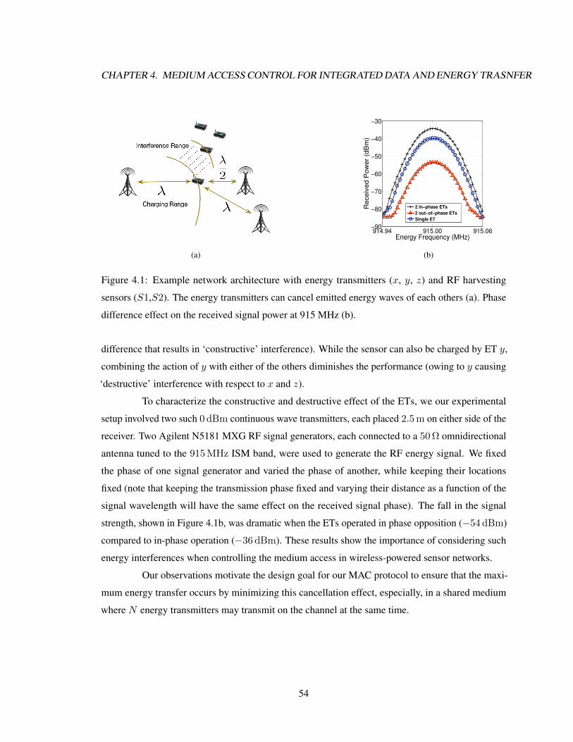
CHAPTER 4. MEDIUM ACCESS CONTROL FOR INTEGRATED DATA AND ENERGY TRASNFER
(a)
914.94 915.00 915.06−90
−80
−70
−60
−50
−40
−30
Energy Frequency (MHz)
Receiv
ed P
ow
er
(dB
m)
2 in−phase ETs
2 out−of−phase ETs
Single ET
(b)
Figure 4.1: Example network architecture with energy transmitters (x, y, z) and RF harvesting
sensors (S1,S2). The energy transmitters can cancel emitted energy waves of each others (a). Phase
difference effect on the received signal power at 915 MHz (b).
difference that results in ‘constructive’ interference). While the sensor can also be charged by ET y,
combining the action of y with either of the others diminishes the performance (owing to y causing
‘destructive’ interference with respect to x and z).
To characterize the constructive and destructive effect of the ETs, we our experimental
setup involved two such 0 dBm continuous wave transmitters, each placed 2.5 m on either side of the
receiver. Two Agilent N5181 MXG RF signal generators, each connected to a 50 Ω omnidirectional
antenna tuned to the 915 MHz ISM band, were used to generate the RF energy signal. We fixed
the phase of one signal generator and varied the phase of another, while keeping their locations
fixed (note that keeping the transmission phase fixed and varying their distance as a function of the
signal wavelength will have the same effect on the received signal phase). The fall in the signal
strength, shown in Figure 4.1b, was dramatic when the ETs operated in phase opposition (−54 dBm)
compared to in-phase operation (−36 dBm). These results show the importance of considering such
energy interferences when controlling the medium access in wireless-powered sensor networks.
Our observations motivate the design goal for our MAC protocol to ensure that the maxi-
mum energy transfer occurs by minimizing this cancellation effect, especially, in a shared medium
where N energy transmitters may transmit on the channel at the same time.
54

CHAPTER 4. MEDIUM ACCESS CONTROL FOR INTEGRATED DATA AND ENERGY TRASNFER
4.3.2 Optimal Frequency and Distance Separation
We next find the optimal frequency separation of the continuous wave ETs and their
respective distances from the energy requesting sensor. Our RF-MAC protocol will use these results
in setting the transmission frequency and activating only those ETs that result in out-phase energy
transfer. Our approach here is to group the ETs together into two sets. All ETs in a given set transmit
at the same center frequency. The two transmission frequencies corresponding to the two groups
are only slightly separated (the complete spectrum of an ET spans only a few KHz). We describe
next how to classify the ETs into separate groups using phase mismatch, such that their cumulative
spectrum spread is still contained within the bandwidth of the energy harvesting (EH) circuit of the
sensor node.
4.3.2.1 Optimal phase mismatch
We first perform a set of experiments to determine how much of the phase mismatch
between two ETs is actually harmful. If the ETs are not completely π radians separated in phase,
then some of them may even be allowed to transmit together. The resultant increase in the raw
emitted power in these cases compensates for the loss owing to the slight mismatch. Figure 4.2a
shows the effect of phase difference ∆φ between two energy transmitters on the received signal
power at 433 MHz and 915 MHz. The experimental setup is the same as for Fig. 1(b). Here, the
phase difference is varied from [0, π] radians. A phase difference of 0 or 2π for the received signal
(the emitted signals being in-phase), corresponds to a linear distance of one wavelength between the
two transmitters. Thus, depending upon the actual distance L between the ET x and receiver node,
we represent φx = Lλ · 2π. Here, λ is the wavelength of the transmitted radiation. From Figure 4.2a,
we observe that for small phase difference, i.e., for ∆φ ≤ π2 , the resultant signal signal strength is
not significantly lowered (i.e., the fall is only about 1− 2 dBm). This determines the optimal phase
separation that is an important parameter in the protocol level design. Accordingly, all those ETs
that are separated by ∆φ ≤ π2 can be grouped under one category (and center its transmissions at
frequency f1, say). Similarly, ETs that are separated by π2 ≤ ∆φ ≤ π fall in the second category (and
use frequency f2 as the center transmission). We call this method as the two-tone energy transfer.
4.3.2.2 Optimal distance separation
In Figure 4.2b, using the experimental results and the relationship between the phase and
distance, all the ETs separated by a multiple of the wavelength from each other, i.e., L = mλ,
55

CHAPTER 4. MEDIUM ACCESS CONTROL FOR INTEGRATED DATA AND ENERGY TRASNFER
0 π/4 π/2 3π/4 π−55
−50
−45
−40
−35
−30
−25
−20
Phase difference (radian)
Receiv
ed P
ow
er
(dB
m)
433 MHz
915 MHz
(a)
!"#$%#&'()*+,-)
.#'#/0#1)234#")*156-))
!"# !$#
∆!#
7+)'/"'%/89:)
;"#$%#&'()
"#:<3&:#=)%&!'#
234#"):<#'8">?)
1#&:/8(=)("&!'#
)*+,,+-.*#/+0123#γ#
234#"):<#'8">?)
1#&:/8(=)($&!'#
ε## ε##
(b)
Figure 4.2: Effect of energy waves phase difference on the received signal power at different
frequencies. The power of resulting wave drops significantly after π/2 phase separation (a). The
scheme for two-tone wireless energy transfer (b).
m = 1, 2, ... can transmit on f1, while the others separated by L = (m + 1/2)λ can transmit on
frequency f2. As there are two active transmission tones present concurrently during transmission,
each of these are separated in the frequency domain, one on each side of the center response point
of the harvesting circuit. Both these tones must be completely encompassed by the response of the
harvesting circuit at the receiver side.
We can potentially group the ETs into more than two categories. However, it can be
observed from Figure 2(a) that increasing the number of groups, results in a smaller phase difference
between ETs. This results in insignificant constructive effect (i.e. about 2 dBm) on the received
signal power. For example, if three groups of ETs are to be employed, the decision region will be
λ/3 and the received signal power is only slightly affected by π/3 phase mismatch. On the other
hand, increasing the number of groups will increases the chance of more destructive interference,
especially for EH circuit with narrow bandwidths. More groups also increase hardware complexity
and energy transfer delay, which are described later in Section 4.5.1. Also, it noteworthy that the
99% occupied bandwidth of the currently used Powercaster ET is relatively small, approximately
63 kHz, thereby allowing us to accommodate the entire transmission spectrum of the ET within the
900 MHz frequency response curve of the EH circuit we designed in [1].
56

CHAPTER 4. MEDIUM ACCESS CONTROL FOR INTEGRATED DATA AND ENERGY TRASNFER
4.3.3 Energy Charging Time
As ETs transmit at comparatively higher energy levels in the same band (34 dBm using
Powercaster transmitter [126] in our testbed, compared to −20 dBm for the Mica2), a much larger
area is rendered unusable for data communication. For example in Figure 4.1a, even if S2 is situated
at a considerable distance away from ET x, it will still fall within its interference band (shown by the
area with dotted lines) and unable to receive data. Thus, the sensor nodes need to balance between
the communication and charging times so that (i) prevent extend durations of communication outage
and (ii) allocate charging durations per energy request based on the traffic load to adaptively sync the
energy harvesting and consumption demands. Accordingly, the effective duration for which charging
is allowed plays an important role in the performance and design of a new MAC protocol.
4.3.4 Requesting and Granting Energy
In a network with multiple ETs, the process of requesting energy by the sensor nodes and
granting energy by the ETs require a timely coordination and cooperation. The MAC protocol must
decide (i) when and how a sensor should actually request energy from neighboring ETs, (ii) when
the ETs should start transferring energy, (iii) how ETs know about suitable charging duration and the
choice of frequency need to be addressed.
4.3.5 Data vs. Energy Channel Access
At the time the sensor node sends the RFE, the residual energy of the requesting node is
very low. Thus, the medium access control should give higher priority to energy requests over data in
the channel access. This design issue is not incorporated into the classical MAC protocols, and needs
to be carefully considered in the design of RF-MAC. Note that issues such as when, how long, and
how frequently ETs access to the channel are determined by charging time and energy requesting
and granting process.
4.4 RF-MAC Protocol Overview
At a high level, the medium access control mechanism in the RF-MAC protocol is organized
into three components - (i) joint ET-spectrum selection, (ii) adaptive charging threshold selection,
and (iii) energy-aware access priority. We now give an overview the RF-MAC protocol, and in the
next section, we describe its detailed operation.
57

CHAPTER 4. MEDIUM ACCESS CONTROL FOR INTEGRATED DATA AND ENERGY TRASNFER
S1(Eres=2.6 v)
BackoffS2S1(Eres=3.0 v) DATA
S1 frozen backoff time
BackoffS1
S2
(Eres=2.3 v) RFE
SIFS
RF MAC energy optimizationDIFSdata
DIFS SIFS
ACKACK
DATA
ACK
S3 remaining backoffB k ff
DIFSdata
DATA
S3(Eres=3.0 v)
SIFSdata
Charging period
S3(Eres=2.8 v)
DIFSenergy
BackoffS3 DIFSdata
SIFSdataS3 remaining backoff
BackoffS2
DIFSdata BackoffS3
S3 frozen backoff time S3 frozen backoff time
Figure 4.3: Example scenario for overview of RF-MAC protocol with three RF energy harvesting
sensor nodes.
• Joint ET-spectrum Selection: In this phase, the energy requesting node issues its request
for energy (RFE) packet. The ETs that receive this request independently separate themselves into
two groups slightly separated in the center frequency, but still contained within the transmission
band. The ETs use the signal strength of the RFE to estimate their (rough) individual distances to the
requesting sensor to identify in which group they belong (see Section 4.3.2) and reply with a cleared
for energy (CFE) pulse. Depending upon which group of ETs supplies higher level of energy, the
requesting sensor solves an optimization framework to assign center frequencies to these two groups.
This technique incorporates consideration of the (i) the destructive effect (i.e. energy cancellation)
of concurrent energy transmissions, and (ii) the spectrum response of the EH circuit, which is an
important physical layer characteristic.
• Adaptive Charging Threshold: In this phase, the energy requesting sensor node de-
termines its upper charging level threshold and the charging duration, based on its local network
conditions. This threshold is unique for a given node, and is derived from the ratio of its own data
communication activity to that observed in its neighborhood. The charging duration determines how
long the data communication should be disrupted.
• Energy-aware Access Priority: This phase has two main functionalities. First, it gives
higher priority to the energy request packets than the data packets for accessing the channel by
defining different durations for the slot time for data and energy access. The slot time is the
fundamental time unit for channel access and exponential back off calculations in CSMA/CA.
Second, it adapts the sensor’s back-off duration based on its residual energy. Thus, the sensor with
higher residual energy has a higher access priority for data communication.
58

CHAPTER 4. MEDIUM ACCESS CONTROL FOR INTEGRATED DATA AND ENERGY TRASNFER
Requesting for Energy
Grouping ETs
Computing Harvestable Power
Spectrum Selection Optimization
Spectrum Confirmation
Sensor Node
Residual Energy
RFE
CFEPackets
Energy Cancellation
Power Spectral Density
Spectrum Response
of EH Circuit
Energy Transfer Frequencies
ACK
Figure 4.4: Five stages of joint ET-spectrum selection component in RF-MAC protocol.
4.4.1 Example Operation of RF-MAC
As an example, in Figure 4.3, three sensors S1, S2, and S3 have residual voltages of 2.6,
2.3, and 3.0 V, respectively. Since the voltage of S2 is reached a pre-set threshold, 2.3 V, this node
sends out the RFE packet requesting for immediate charging. RF-MAC, through the access priority
mechanism (Section 4.5.3), ensures that S2 wins the channel access for energy transfer earlier than
S1 and S3 that have data packets to deliver. At this time, S1 and S3 are forced to freeze their backoff
timers and get into charging mode, as data communication is infeasible. Once RFE packet is received
by the ETs, they reply back with the CFE, which is a short energy pulse.
Node S2 identifies the two sets of ETs by measuring the received power of CFEs and
determines their associative optimal energy transfer frequencies (Section 4.5.1). How much should
S2 charge depends upon the adaptive charging threshold selection (Section 4.5.2). The node S2
then sends out an ACK packet to the ETs in which it includes the optimal frequencies as well as the
charging duration. Finally, when nodes S1 and S3 compete for data transfer, access priority ensures
their respective backoff windows are a function of the residual energy (Section 4.5.3). Assuming that
S1 has higher residual energy, it will likely get the data communication opportunity first, followed by
S3. The latter freezes the countdown timer in this duration, and resumes the remaining countdown
as soon as the channel is next available.
The details of the above three phases and the complete RF-MAC protocol description is
given in the next section.
59

CHAPTER 4. MEDIUM ACCESS CONTROL FOR INTEGRATED DATA AND ENERGY TRASNFER
!"#$%&'λ()("(*(+,($,(&,(-(
("λ()("(*(+,($,(&,(-(
./$(
./&(
./0(
./1(
./2(
./3(
./4(
./5(
./6(
(789:;:<=(><?=@ABC(
(a)
21
Charging time
S1
ET 1
ET 2
ET 3
ET 4
ET 5
ET 9
mλ : m = 0, 1, 2, !
(m+1/2)λ : m = 0, 1, 2, !
RFE ACK
Slot number
Energy pulses
Slot time
(b)
Figure 4.5: Grouping and selection of ETs based on the destructive interference of energy waves (a),
the timing diagram for requesting and granting energy in the RF-MAC protocol (b).
4.5 Detailed RF-MAC Protocol Description
4.5.1 Joint ET-spectrum Selection
As shown in Figure 4.4, the specific stages considered during the joint ET-spectrum
selection are (i) requesting for energy, (ii) grouping ETs based on destructive interference, (iii)
computing harvestable power, (iv) spectrum selection optimization, and (v) spectrum confirmation.
4.5.1.1 Requesting for energy
The sensor node broadcasts the RFE packet, requesting for energy, when its voltage falls
under a pre-set threshold (∼ 2.3 V, as minimum operating voltage of the Mica2 is 1.8 V). The RFE
contains the requesting sensor node’s ID, transmitted at constant signal strength. This RFE can
be sent when the channel is free, i.e., when there is no ongoing data transfer or energy charging
operation and the channel lies idle for the DIFSenergy duration (calculation of this channel sensing
duration is described later in Section 4.5.3). The ETs that receive this packet estimate roughly their
distances from the node, based upon the received signal strength (RSS). In the following, we define
that the distance measurement only needs to determine a band in which the ET lies, and not its exact
location.
60

CHAPTER 4. MEDIUM ACCESS CONTROL FOR INTEGRATED DATA AND ENERGY TRASNFER
4.5.1.2 Grouping ETs based on destructive interference
Recall from Section 4.3, the distance between the ET and the sensor node directly results
in a phase difference of the incoming wireless signals at the node. The ETs that identify themselves
to lie in the band [mλ− λ4 ,mλ+ λ
4 ], are grouped together, where m = 1, 2, .... We call this as
Group I. Similarly, the other ETs in the range [(m + 1/2)λ − λ4 , (m + 1/2)λ + λ
4 ] fall in the
second group, called Group II. Thus, on receiving the RFE, each ET knows which concentric
band it lies in centered around the requesting node, and the group in which it belongs. Figure 4.5a
shows a sample scenario. The shaded region depicts the ETs 4 and 5 that lie in the band of λ, i.e., in
Group I. This region extends up to λ4 on either side of the central bold line that lies at an exact
distance of λ with the requesting node placed at the center. Since we do not precisely require the
ET to calculate the distance from the requesting node, but only need to determine if it lies within
a concentric band-region, our approach is more robust to RSS fluctuations. Of course, using a
dedicated localization scheme or GPS hardware considerably eases this constraint, though adding to
the implementation cost and power requirement.
The ETs that hear the RFE reply back with a single and constant energy pulse. Each
concentric band has the choice of one of two time slots in which this pulse may be emitted, beginning
from the instant of completion of the RFE, as shown in Figure 4.5b. Referring again to the band
structure in Figure 4.5a, the first slot is allocated for CFE pulses sent by energy transmitter of Group
I (note: all Group I bands are shown shaded). Similarly, CFE pulses from energy transmitters of
Group II are sent during the second slot, i.e. ETs 1, 2 and 3 collectively lie in the second concentric
(Group II) band and simultaneously transmit their pulses in the second slot.
4.5.1.3 Computing harvestable power
The node that sent the initial RFE estimates the total energy that it will receive based on the
signal strength of the CFE pulses in the slot number in which they were received. This arrangement
of using the pulses allows the ETs to be simple in design, and removes the concern of collisions.
Unlike classical data communication, it is not important for the node to know which ET will transmit
energy. Rather, its energy calculations are based on how much energy is contributed by the two
groups of ETs separately. We define this cumulative energy as EGroup IRX and EGroup IIRX , respectively,
which are calculated by the RFE issuing node from the received pulses. Each slot time is 10µs in
our work, allowing a very fast response time. The purpose of differentiating the energy contribution
from the two groups is useful in the next stage, where an optimization function returns the center
61

CHAPTER 4. MEDIUM ACCESS CONTROL FOR INTEGRATED DATA AND ENERGY TRASNFER
frequencies of the ETs.
4.5.1.4 Spectrum selection optimization
Let Group I ETs be centered at frequency f1, and Group II ETs be centered at
frequency f2 so that they can concurrently transfer energy without destructively affecting each other.
How to select these frequencies f1 and f2 is explained next, which takes into account two important
physical layer characteristics of the energy transfer. The first is the spectrum response of the energy
harvesting circuit that is connected to the sensor nodes, shown by the envelope H(f) in the frequency
domain in Figure 4.2b. The physical bandwidth of energy harvesting circuit is denoted by BWEH .
The power spectral density (PSD) of the two groups of ETs is the other concern, represented by S1(f)
and S2(f), respectively, for Group I and Group II. The sensor node observes these shapes from
the incoming pulses from the ETs. Thus, the bandwidth 2ε of the transmission spectrum (centered
at f1 and f2) must be selected in such a way there is a minimum overlap between their individual
spectra, and yet contained within the envelope of H(f). We use the following optimization if the
transmission spectrum of the ETs occupies a bandwidth of 2ε.
The aim of the optimization formulation is to maximize the energy transfer EMaxRX =
EGroup IRX + EGroup IIRX , which at a given frequency point is the product of the power spectral density
and the circuit frequency response. Thus, the useful components that need to be maximized are the
first two terms of (4.2), which give the constructive energy contribution of the ETs of the two groups.
Given : S1(f), S2(f), BWEH , H(f)
To find : f1, f2, γ (4.1)
To Maximize :
EMaxRX =
∫ f1+ε
f1−εS1(f)H(f)df +
∫ f2+ε
f2−εS2(f)H(f)df
− (
∫ γ
f2−εS2(f)H(f) df +
∫ f1+ε
γ
S1(f)H(f) df)︸ ︷︷ ︸destructive interference
(4.2)
Subject to :
|f2 − f1| < BWEH (4.3)
d(S1(f)H(f))
df
∣∣∣f=γ
< 0 (4.4)
d(S2(f)H(f))
df
∣∣∣f=γ
> 0 (4.5)
62

CHAPTER 4. MEDIUM ACCESS CONTROL FOR INTEGRATED DATA AND ENERGY TRASNFER
The first constraint is to ensure that both frequency groups are contained within the
bandwidth of the energy harvesting circuit. The constraints 4.4 and 4.5 ensure that the spectrum
shapes of the Group I and Group II ETs does not overlap completely. We assign f1 to the left
of f2 on the frequency scale (see Figure 4.2b). At the point of the intersection of the PSD curves
S1(f) and S2(f), which we call the cross-over point γ, the slope of the curves must be positive and
negative, respectively. This is calculated by differentiating the respective PSD plots at γ, to ensure
that one of them increases (positive slope) while the other falls (negative slope). A problem is said
to have an optimal substructure if an optimal solution can be constructed efficiently from optimal
solutions to its sub-problems. We claim as follows that our proposed optimization also exhibits the
optimal substructure property.
Lemma 1: Given the power spectral density S1(f) and S2(f), the total energy transfer
(EMaxRX ) under the RF energy harvesting circuit’s frequency response H(f) is maximum.
EMaxRX =
∫ f1+ε
f1−εS1(f)H(f)df︸ ︷︷ ︸
(1)
+
∫ f2+ε
f2−εS2(f)H(f)df︸ ︷︷ ︸
(2)
− ∫ γ
f2−εS2(f)H(f)df︸ ︷︷ ︸
(3)
+
∫ f1+ε
γ
S1(f)H(f)df︸ ︷︷ ︸(4)
is maximum then∫ f1+ε
f1−εS1(f)H(f)df −
∫ γ
f2−εS2(f)H(f)df︸ ︷︷ ︸
X
and
+
∫ f2+ε
f2−εS2(f)H(f)df −
∫ f1+ε
γ
S1(f)H(f) df︸ ︷︷ ︸Y
are maximum as well
Proof: Let (1)−(3) give the area under the curve represented by X and (2)−(4), similarly,
return the area of Y, then (1) + (2)− (3) + (4) has the total area of X+Y. Assume we find α such
that α = (1)−(3)+ε ; ε > 0 then the total area = (1)+(2)−(3)+(4)+ε = X+Y +ε > X+Y .
This contradicts the supposition that (1) + (2)− (3) + (4) is maximum. (1)− (4) can be proved
in a similar fashion.
63

CHAPTER 4. MEDIUM ACCESS CONTROL FOR INTEGRATED DATA AND ENERGY TRASNFER
4.5.1.5 Spectrum confirmation
With the resulting dual-frequency wireless energy transfer, both groups of ETs can be
simultaneously active. The final part of this stage involves letting the ETs know that they are cleared
for energy transmission through an Acknowledgement (ACK) packet. This packet provides the ETs
the center point for the frequencies f1 and f2, according to the results of optimization. The ETs know
which group they belong to internally, based on the RSS-based band structure shown in Figure 4.5a.
Additionally, the ACK carries an estimated charging time T based on a target voltage level of the
capacitor (calculated in Section 4.5.2). This upper limit on the charging voltage is decided by the
node’s relative activity in the neighborhood.
After a short SIFS wait period following the ACK (using shorter slot times, for energy,
compared to those used for data communication), the ETs begin their transmission. In case of loss
of the RFE due to packet collision or bad channel conditions, the contention windows are re-set
to the minimum width, thereby initiating an immediate subsequent retry. The idea here is that (i)
time is critical when a node has extremely low voltage and (ii) nodes will require energy recharging
opportunities much less than the data communication opportunities [148]. Hence, the number of
energy request packets will be less than data packets and there will not be frequent collision related
losses of the RFE arising from the shorter contention window.
From our preliminary experimental results, we recall that increasing the number of groups
to more than two has negligible constructive effect on the received signal power (see Section 4.3.2.2).
In addition to this, we find that introducing an additional frequency group, say Group III with
PSD S3(f), increases the chance of more destructive interference, and in the optimization formula
the destructive interference term increases from 2 terms (all overlapping areas of S1(f) and S2(f))
to at least 4 terms (all overlapping areas of S1(f), S2(f), S3(f)). Furthermore, as the number of
groups increases the number of slot times for CFE pulses and computing the harvestable power also
increases. Clearly, this results in additional delay in granting energy to the sensor nodes. Finally,
more than two groups of energy transmitters mean tighter location detection requirement and hence
most likely more expensive hardware.
4.5.2 Adaptive Charging Threshold
As our energy transfer is in-band, each node needs to decide the charging time that maypossibly result in a reduced level of energy replenishment. Our proposed method defines this uppercharging level based on the level of participation in data communication activity for that node
64

CHAPTER 4. MEDIUM ACCESS CONTROL FOR INTEGRATED DATA AND ENERGY TRASNFER
with respect to its neighbors. Each node maintains a moving average of the time spent by itselfin transmitting and receiving data packets to the total time the channel is used or sensed as busy.Many nodes, hence, will never charge to their maximum capacity, and thereby, they sacrifice theircharging opportunity for the larger good of the network performance. The node’s importance index
(IDX) is shown in (4.6), where Tx represents the number of data packets that originate from it and Rx
denotes the number of packets destined for the node. Data transfer activity, overhead by the node,that neither originate nor end at it are expressed through Channel busy time. The upper chargingvoltage V threshold
max is calculated from (4.7).
IDX =Tx+Rx
Tx+Rx+ Channel busy time(4.6)
V thresholdmax = IDX × (Vmax − Vmin) + Vmin (4.7)
The charging time T that the node includes in the ACK is calculated as follows, using the standard
definitions of energy stored in the capacitor, (4.7) and the trigger voltage V thresholdmin under which the
RFE is set out by the node.
T =1
2C(V thresholdmax )2 − (V thresholdmin )2)2Slotenergy
EMaxRX
(4.8)
Here, the received energy during the CFE pulses is obtained from two successive time
slots, each of duration Slotenergy.
4.5.3 Energy-aware Access Priority
This channel access determining feature of the RF-MAC manifests in two ways: The first
is prioritizing between energy transfer and data communication, and secondly, identifying which
nodes within the network should send out the data packets first by winning the channel.
4.5.3.1 Energy transfer prioritization
The residual energy of the requesting node is below a threshold V thresholdmin when it sends
the RFE, and hence, it should have higher priority in channel access. This is ensured by separately
defining the DIFS duration for energy and data. Consequently, the specially formulated energy
request DIFS duration (DIFSenergy) is shorter than DIFS for data exchange (DIFSdata), achieved by
assigning a shorter slot time for energy request, while data exchange is provisioned with a longer
slot time. Hence, we use the slot time of 10µs for energy request and 20µs for data communication
as defined in the 802.11 standard [137]. Since DIFS is defined as SIFS + 2Slot timeenergy, we
65

CHAPTER 4. MEDIUM ACCESS CONTROL FOR INTEGRATED DATA AND ENERGY TRASNFER
derive 25 µs for DIFSenergy and 50 µs for DIFSdata. With the shorter DIFS duration and slot time,
RF-MAC prioritizes the energy request over data exchange. Note that DIFS and SIFS are defined
acronyms in 802.11 standard [137]. The time calculations for the protocol are given in Table I.
Parameter Value
slot time 10µs (energy), 20µs (data)
CWmin 32
CWmax 1024
DIFSenergy SIFSenergy + 2Slot timeenergy = 25 µs
DIFSdata SIFSdata + 2Slot timedata = 50 µs
SIFS 5 µs (energy), 10 µs (data)
Table 4.1: Parameters used in RF-MAC
4.5.3.2 Data transfer prioritization
In the data exchange phase, the sensor contends for a channel using the CSMA/CA
mechanism defined in 802.11 [137], i.e., it senses the channel for the DIFS duration before attempting
a transmission. Consequently, sensors with higher energy harvesting rate, owing to their position or
channel characteristics between the ETs and themselves, will have shorter charging durations. They
will be able to participate timely for data communication, without interruptions and packet drops for
frequent replenishment of energy, all of which contribute to the energy usage. We assign sensors with
higher residual energy level a correspondingly higher priority to transmit. [149] proves analytically
that this method results in an asymptotically optimal network lifetime. We design RF-MAC in such
a way that the sensor’s backoff duration is influenced by its residual energy, i.e., the node with
higher residual energy experiences a shorter backoff duration than the node with lower residual
energy. An example of the adaptive backoff mechanism for data exchange is described in (4.9). The
contention window for data exchange (CWdata) is randomly selected from the range between the
minimum CW and node’s current CW , [CWmin, CWcurrent]. We set the contention window of 32
for CWmin in this work. Further, (4.9) shows how the effective slot time is a scaled value based on
the residual energy. The capacitor voltage is used for scaling, where it is limited at the high end by
the rated voltage of the capacitor Vmax (note this is different from the upper charging threshold in
66

CHAPTER 4. MEDIUM ACCESS CONTROL FOR INTEGRATED DATA AND ENERGY TRASNFER
S1 (Eres= 2.8 v)
ACK
DATA 3 2 1
3
2 5 4
2 1
1
S2 (Eres= 3.0 v)
S3 (Eres= 3.0 v)
S4 (Eres= 2.6 v)
5 4
3 6
DATA
ACK
DATA
ACK
SIFSdata
Remaining backoff time
SIFSdata
SIFSdata DIFSdata
DIFSdata
DIFSdata
Frozen backoff time
Figure 4.6: Energy-aware data exchange process in RF-MAC protocol with three transmitter nodes
S1, S2, and S4 and the receiver node S3.
(4.7), current voltage Vcurrent, and the V thresholdmin that signals a critical point if the sensor needs to
be kept in operation.
Backoff = DIFSdata + CWdata × Slotenergy+
(Vmax − Vcurrent)(Slotdata − Slotenergy)
Vmax − V thresholdmin
︸ ︷︷ ︸adaptive slot time
(4.9)
The overall process of data exchange is explained using Figure 4.6. Sensors S1, S2, and
S4 all have packets to transmit to sensor S3 at the start (indicated by the arrow on the time axis).
They each sense the channel for DIFSdata. Intuitively from (4.9), sensor S2 with the residual energy
of 3.0 v, should experience the shortest backup duration, as opposed to S1 and S4. However, this
does not imply that the nodes with higher residual energy will always have a shorter back off duration,
as the random selection of the backoff slots within the window does contribute to the overall backoff
time. This selection of the window [CWmin, CWcurrent] is independent of node’s residual energy.
4.6 Simulation Results
In this section, we evaluate the performance of our RF-MAC protocol using the ns-2
network simulator, with experimental results presented in the next section. We demonstrate the
performance improvement with respect to the following metrics: (i) number of energy transmitters,
(ii) number of data flows, (iii) numbers of nodes, and (iv) packet size. The primary performance
metrics are the average network throughput and the average harvested energy. In particular, the first
67

CHAPTER 4. MEDIUM ACCESS CONTROL FOR INTEGRATED DATA AND ENERGY TRASNFER
metric shows the average per-node throughput of the sensor network, and the second metric gives the
average energy harvested per-node that is found by recording and averaging the harvested power by
nodes during the simulation.
The simulation parameters are set as follows. The EH circuit parameters are from [1].
We model the ETs on the Powercaster transmitter [126], which radiates continuous waves at 3 W.
The operational characteristics of the sensor, such as energy spent on transmission, reception, idle
listening, channel bandwidth, etc. are from Mica2 specifications [150]. Unless specifically stated,
250 sensor nodes and 100 ETs are deployed uniformly at random in 50 x 50 m2 grid. Traffic loads
are generated by constant bit rate (CBR) flows. Nodes have a full buffer and all data packets are 50
bytes in size. The sender/receiver pairs are chosen randomly, and the intermediate relaying nodes do
not aggregate or compress data. Additional parameters used in the simulation are presented in Table
I.
We compare three different protocols: 1) RF-MAC-opt, 2) RF-MAC-no-opt, and 3) modi-
fied unslotted CSMA. RF-MAC-opt is the full-featured RF-MAC, including the joint spectrum-ET
selection, adaptive charging threshold, and energy-aware channel access priority mechanisms, as
discussed in Section 4.4. The RF-MAC without the optimization (named RF-MAC-no-opt) has all
components of RF-MAC other than joint spectrum-ET selection component. In particular, it does not
assign different frequencies to the ETs and makes no attempt to identify and classify ETs based on
their phase mismatch. We evaluate the RF-MAC-opt against RF-MAC-no-opt in order to investigate
the effectiveness of the joint spectrum-ET selection feature incorporated in our RF-MAC protocol,
especially in avoiding energy interference and improving the network performance. Finally, the
modified CSMA is adapted from [105], which provides the baseline for our performance evaluations.
To have a fair baseline comparison, the modified CSMA (in which each sensor node may issue the
RFEs and receive the CFEs) is compared against both RF-MAC-opt and RF-MAC-no-opt. In the
modified CSMA, there is no attempt made to calculate the optimal charging time, and it has none of
the features of the RF-MAC protocol. Once an RFE is sent out, the node charges to its maximum
capacity and does not take into consideration the impact on data traffic, energy cancellation, and the
residual level of the sensor nodes. Data points in each graph represent the mean of twenty scenarios
and the corresponding 95% confidence intervals are plotted as error bars in the figures.
68

CHAPTER 4. MEDIUM ACCESS CONTROL FOR INTEGRATED DATA AND ENERGY TRASNFER
0
2
4
6
8
10
12
14
16
18
1 2 3 4 5 6 7 8 9 10 11 12
Avera
ge H
arv
este
d E
nerg
y (
Joule
s)
ET Density (n)
RF-MAC-optRF-MAC-no-optModified CSMA
Figure 4.7: Effect of the number of ETs on the average harvested energy.
4.6.1 Impact of the Number of ETs
In the first set of experiments, we investigate the effect of the number of ETs for different
MAC protocols. Figure 4.7 shows the effect of the ET density on the average harvested energy of two
RF-MAC variants. The ET density, defined as the average number of ETs located within the radio
range of a sensor node, varies from 1 to 12. It is clear that both RF-MAC variants dominate over the
modified CSMA. As shown in Figure 4.7, RF-MAC-opt delivers monotonically increasing average
harvested energy with increasing the number of ET density. The benefit of frequency optimization
greatly improves the performance as it maximizes the energy transfer by separating two transmission
spectrum and ensuring the highest level of energy delivery. Without this optimization, ETs enter the
charging process and do not take into account the possibility of destructive interference, resulting in
sub-optimal energy transfer.
The average network throughput is shown in Figure 4.8 and the trend is observed to be very
similar to the average harvested energy plot. Both variants of RF-MAC yield higher average network
throughput as ET density increases. However, the throughput of RF-MAC-opt is significantly higher
that RF-MAC-no-opt, with a 62% increase on average. Both the average harvested energy and
average network throughput of modified CSMA are the lowest among protocols under study. This
is because modified CSMA does not have the adaptive charging features included in the RF-MAC
protocol. In this case, RF-MAC-opt yields over 100% and 300% more than the modified CSMA in
terms of the average harvested energy and average throughput, respectively.
69

CHAPTER 4. MEDIUM ACCESS CONTROL FOR INTEGRATED DATA AND ENERGY TRASNFER
0
50
100
150
200
250
300
350
400
450
500
1 2 3 4 5 6 7 8 9 10 11 12
Avera
ge N
etw
ork
Thro
ughput
(Byte
s/s
)
ET Density (n)
RF-MAC-optRF-MAC-no-optModified CSMA
Figure 4.8: Effect of the number of ETs on the average network throughput.
4.6.2 Impact of Multiple Flows
The effect of multiple simultaneous flows in the sensor network is investigated next, with
random selection of source and destination nodes, while the number of flows is varied from 1
to 6. Again, we observe the behavior of RF-MAC on two energy and throughput metrics, when
nodes experience different levels of channel usage and traffic loads. Figure 4.9 shows a smooth
and monotonic increase in the average harvested energy of RF-MAC-opt as the number of flows
increases. Even though the RF-MAC-no-opt exhibits a similar pattern, the increase is not as smooth
as one with the frequency optimization. Evidently, the amount of average harvested energy yield
could be almost 150% less than RF-MAC-opt. Figure 4.10 depicts the average network throughput
of RF-MAC with various numbers of data flows. Interestingly, the average network throughput
of both RF-MAC variants gracefully drops as the number of data flow increases. This reduction
in the throughput is a result of more nodes sending out RFEs as they deplete their energy faster
with increasing number of data flows. Consequently, the network spends more time in the charging
state and less time spent in the data exchange state. However, RF-MAC-opt yields higher average
network throughput, approximately 20% more in this case. Again, both variants of RF-MAC largely
outperform the modified CSMA. Especially, RF-MAC-opt yields approximately 112% increase in
terms of throughput.
70

CHAPTER 4. MEDIUM ACCESS CONTROL FOR INTEGRATED DATA AND ENERGY TRASNFER
5
6
7
8
9
10
11
12
13
14
1 2 3 4 5 6
Avera
ge H
arv
este
d E
nerg
y (
Joule
s)
Number of Flows
RF-MAC-optRF-MAC-no-optModified CSMA
Figure 4.9: Effect of multiple flows on the average harvested energy.
4.6.3 Impact of the Number of Sensor Nodes
We investigate how RF-MAC protocol behaves when the number of sensor nodes in the
topology changes. We randomly deploy various numbers of sensor nodes in the topology, ranging
from 60 to 240. The average harvested energy is shown in Figure 4.11, wherein the performance of
RF-MAC-opt smoothly drops and tends to stabilize when 120 sensor nodes or more are present. On
the other hand, RF-MAC-no-opt yields a similar pattern to the modified CSMA, a rather constant
average harvested energy with fluctuations around the mean trend. Again, RF-MAC-opt offers
higher average harvested energy when compared to RF-MAC-no-opt. Figure 4.12 depicts the
average network throughput of RF-MAC with different numbers of sensor nodes. Similar to the
earlier case with the average harvested energy, both RF-MAC variants experience the reduction in
average network throughput even RF-MAC-opt displays marginally higher throughput. Moreover,
the modified CSMA performs significantly lower than RF-MAC-opt and RF-MAC-no-opt in both
harvested energy and network throughput.
4.6.4 Impact of Packet Size
The packet size is varied from 30 to 90 bytes with an increment of 20 bytes, while other
parameters are kept to their default settings. The impact of packet size on the average harvested
energy of RF-MAC is shown in Figure 4.13. It is clear that the average harvested energy of RF-
MAC-opt is monotonically increasing with an increasing packet size, and offers up to 25% gain over
71

CHAPTER 4. MEDIUM ACCESS CONTROL FOR INTEGRATED DATA AND ENERGY TRASNFER
0
20
40
60
80
100
120
140
1 2 3 4 5 6
Avera
ge N
etw
ork
Thro
ughput
(Byte
s/s
)
Number of Flows
RF-MAC-optRF-MAC-no-optModified CSMA
Figure 4.10: Effect of multiple flows on the average network throughput.
RF-MAC-no-opt at the packet size of 90 bytes. On the other hand, the average harvested energy
of RF-MAC-no-opt tends to stabilize for packet sizes larger than 50 bytes. The average network
throughput of RF-MAC is shown in Figure 4.14. Both RF-MAC variants offer an increase in average
network throughput with increasing packet size. Again, the RF-MAC-opt outperforms, in terms of
the average network throughput, its non-optimized variant and the modified CSMA throughout the
study range.
4.7 Experimental Study
Our testbed consists of 4 parts, signal generators (Agilent N5181 MXG RF signal gener-
ators), RF switches, RF amplifiers of 3W EIRP (to emulate two ETs), and three wireless sensors.
We implemented the RF-MAC protocol in Mica2 motes equipped with Chipcon CC1000 radios
and connected to our in-house fabricated RF energy harvester [1] operating at 915MHz shown in
Figure 4.15. The sender motes are programmed to continuously transmit 30 Byte packets to the sink.
We use the following setup to build the two ETs for the transmission of wireless RF power, whose
schematic is shown in Figure 4.16. The signal generators produce two energy waves with bandwidth
63 kHz (similar to Powercaster transmitter [126]) that are slightly shifted, corresponding to the
frequencies f1 and f2 obtained in frequency assignment optimization earlier. These frequencies
for our energy harvesting setup are found as f1 = 915 MHz and f2 = 916 MHz. This assures that
transmission of the ETs and the sensor motes are in-band and mechanisms such as data vs. energy
72

CHAPTER 4. MEDIUM ACCESS CONTROL FOR INTEGRATED DATA AND ENERGY TRASNFER
0
2
4
6
8
10
12
14
16
60 80 100 120 140 160 180 200 220 240
Avera
ge H
arv
este
d E
nerg
y (
Joule
s)
Number of Sensor Nodes (m)
RF-MAC-optRF-MAC-no-optModified CSMA
Figure 4.11: Effect of the number of nodes on the average harvested energy.
channel access can be verified correctly through the experiments. The ET controller sends appropriate
interrupt signal to the RF switch upon receiving the ACK packet from the energy requesting node.
We also programmed Mica2 mote to function as an ET controller by using three interrupt pins of the
mote’s expansion connector based on the MPR/MIB User’s Manual[150]. Specifically, INT0 is used
to disable and enable the RF switch, INT1 is used to select output frequency f1, and INT2 is used for
selecting output frequency f2. Accordingly, the RF switch passes the selected input signal to the RF
amplifier which then transmits with output power 3W EIRP. Note that in the testbed both ET1 and
ET2 have the same configurations, with the interior working of one of them expanded for brevity.
In order to verify the benefit of RF-MAC variants (two-tone and single-tone energy transfer)
over the modified CSMA, the RF harvester is fixed at the location 0λ, ET1 is fixed in location 3λ
away from the harvester, while the location of ET2 is varied between location 0λ to 3λ. We evaluate
the testbed under three different scenarios as follows:
• Both ET1 and ET2 adopt RF-MAC with two-tone energy transfer (f1 at 915 MHz and f2 at
916 MHz).
• Both ET1 and ET2 adopt RF-MAC with single-tone energy transfer (only one group is
transmitted on f1 at 915 MHz).
• Both ET1 and ET2 adopt the modified CSMA that does not employ frequency assignment
optimization.
73

CHAPTER 4. MEDIUM ACCESS CONTROL FOR INTEGRATED DATA AND ENERGY TRASNFER
100
110
120
130
140
150
160
170
180
60 80 100 120 140 160 180 200 220 240
Avera
ge N
etw
ork
Thro
ughput
(Byte
s/s
)
Number of Sensor Nodes (m)
RF-MAC-optRF-MAC-no-optModified CSMA
Figure 4.12: Effect of the number of nodes on the average network throughput.
The average charging time and the network throughput of the testbed under various MAC
protocols are shown in Figures 4.17 and 4.18. Each point in the experimental results represents
an average of ten independent experiments for 95% confidence interval with 5% precision. It is
clear that the RF-MAC with two-tone energy transfer not only yields the highest average network
throughput and the lowest charging time but also it experiences minimal fluctuations. On the other
hand, the modified CSMA gives the highest charging time and the lowest network throughput
when ET2 is not located at the position that results in in-phase combination of energy waves at the
harvester. The RF-MAC protocol prevents destructive effect by out-of-phase combination of energy
waves, and consequently achieves higher average network throughput. Moreover, the RF-MAC with
two-tone energy transfer provides additional improvements in the receiving power when compared
to single-tone energy transfer since both ET1 and ET2 can operate simultaneously. There exists a
region where destructive effect is less pronounced, i.e., when ET2 is varied from location 0λ to 1λ.
This is because the power provided by ET2 is much higher when compared to the one provided by
ET1. ET2 power and phase simply dominates the behavioral outcome. However, it can be observed
that the destructive effect is more pronounced when ETs are distanced equally, i.e. ET2 at 2.5λ or
3.5λ when ET1 is at 3λ.
74

CHAPTER 4. MEDIUM ACCESS CONTROL FOR INTEGRATED DATA AND ENERGY TRASNFER
30 50 70 900
2
4
6
8
10
12
Packet Size (Bytes)
Avera
ge H
arv
este
d E
nerg
y (
Joule
s)
RF−MAC−optRF−MAC−no−optUnslotted CSMA
Figure 4.13: Effect of the packet size on the average harvested energy.
4.8 Final Remarks
In this chapter, we proposed the RF-MAC protocol that specifically addresses the problems
of joint selection of energy transmitters and their frequencies based on the collective impact on
charging time and energy interference, setting the maximum energy charging threshold, requesting
and granting energy, and energy-aware access priority. The grouping of the ETs into two sets with
varying transmission frequencies, and the minimal control overhead are both geared to keep the
hardware requirements simple, and the protocol easier to implement. Our protocol delves on the
important issue of how to determine the energy vs. data communication tradeoff, especially as one
occurs as the cost of the other. Finally, simulation and testbed results reveal that RF-MAC largely
outperforms the modified CSMA in both average harvested energy and average network throughput.
75

CHAPTER 4. MEDIUM ACCESS CONTROL FOR INTEGRATED DATA AND ENERGY TRASNFER
30 50 70 900
20
40
60
80
100
120
140
160
180
200
Packet Size (Bytes)
Avera
ge N
etw
ork
Thro
ughput (B
yte
s/s
)
RF−MAC−optRF−MAC−no−optUnslotted CSMA
Figure 4.14: Effect of the packet size on the average network throughput.
Figure 4.15: Our fabricated RF energy harvester [1] powers Mica2 mote by converting the received
RF power to electrical energy.
76

CHAPTER 4. MEDIUM ACCESS CONTROL FOR INTEGRATED DATA AND ENERGY TRASNFER
Agilent N5181 MXG
RF signal generator
Agilent N5181 MXG
RF signal generator
RF Switch
Amplifier
ET2
ET Controller(Mica2)
INT0
INT1
ET1
f1 f2
INT2
Figure 4.16: Schematic of our experimental setup for transmission of wireless RF power.
0 0.5 1 1.5 2 2.5 30
10
20
30
40
50
ET#2 location (Lambda)
Ch
arg
ing
Tim
e (
Se
co
nd
s)
Dual ETs, RF−MAC Two−toneDual ETs, Modified CSMASingle ET, RF−MAC Single
Figure 4.17: Effect of ET2 position on the average harvested energy.
0 0.5 1 1.5 2 2.5 30.2
0.4
0.6
0.8
1
1.2
1.4
1.6
1.8
ET#2 location (Lambda)
Th
rou
gh
pu
t (K
byte
/s)
Dual ETs, RF−MAC Two−tone
Dual ETs, Modified CSMA
Single ET, RF−MAC Single−tone
Figure 4.18: Effect of ET2 position on the average network throughput.
77

Chapter 5
Omnidirectional RF-Powered Wireless
Sensor Network
5.1 Introduction
In this chapter, we study the omnidirectional RF-powered wireless sensor network and
propose analytical models to capture the behavior and energy interference in such networks. In
particular, we investigate the possibility and effects of concurrent data and energy transfer in the
first section. It follows with an experimental section to show how practically low-power data
communications can survive the presence of high-power energy signals. The last section introduces
an analytical framework to calculate the received and harvestable power from multiple wireless
chargers at each point of space taking into account low-power data communications, RF energy
harvesting circuit, and interference among energy signals.
5.2 Concurrent Data and Wireless Energy Transfer
Wireless Sensor Networks (WSNs) are a fundamental building block of the Internet of
Things (IoT) and a key enabler for cyber physical and pervasive computing systems. However, sensor
nodes are typically battery-powered, and their limited energy affects protocol design, sacrificing
throughput, bandwidth usage, and reliability to the need for extended network lifetime through
judicious use of energy. Since it is often difficult, if not impossible, to access the sensor nodes and
replace their batteries, most research efforts have focused on intelligent duty cycling and energy
78

CHAPTER 5. OMNIDIRECTIONAL RF-POWERED WIRELESS SENSOR NETWORK
saving techniques at all layers of the protocol stack. Recent developments in energy harvesting
technology from ambient sources promise to alleviate some of these concerns [138].
This section explores the scenario where radio frequency (RF)-based technology is used
to charge the sensors through dedicated energy transmitters (ETs). However, the high broadcast
power of the ETs, emitting energy waves up to 3 Watts, introduces additional interference in data
communication. Through detailed experimentation, this section aims at quantifying the impact
of selecting network parameters relevant to RF energy transfer and data communication on the
coexistence of ETs and sensor nodes. In particular, we are interested in determining values of
those parameters that enable fruitful coexistence, considering the challenges imposed by the low
transmission power of the sensor nodes (e.g., the output power of 802.15.4 devices, which is typically
as low as 0 dBm) and the high-power energy waves (possibly above 30 dBm), causing interference
and significant packet loss.
Our experiments involve both the physical layer and the link layer by measuring the
received signal strength, packet reception rate, and the amount of harvested power under carefully-
designed scenarios with single and multiple ETs. Previous empirical studies in WSNs focused
on complex, non-ideal behavior of low-power wireless links [151, 152], concurrent data transmis-
sions [153], and the coexistence between WSNs and WiFi [154, 155], microwave ovens [156] and the
smart grid [157]. To the best of our knowledge, this work provides the first study on interference and
coexistence issues in RF energy-powered WSNs. In so doing, we identify the boundary conditions
that allow nodes equipped with RF energy harvesters to transfer data with high throughput and with
limited interference from transmitting ETs.
The key contributions of our work include the following.
• We investigate the effect of data transmissions and energy transfer in the same frequency
band, quantifying the impact of long-range interference of energy transmitters, and the energy
charging range required to effectively recharge nodes.
• We show the interference between RF energy transmitters and wireless nodes when they occur
simultaneously as a function of the separation of frequency of use. We also identify safe
frequency separation for concurrent data and energy transmission.
• We demonstrate the destructive interference effect of multiple energy transmissions on the
same frequency, and measure the impact of energy cancellation on the amount of harvested
power.
79

CHAPTER 5. OMNIDIRECTIONAL RF-POWERED WIRELESS SENSOR NETWORK
• We show the viability and efficiency of multi-frequency band RF energy harvesting for RF
energy circuits with a wide frequency response range.
The rest of this part is organized as follows. In Section 5.3.1 we describe our experimental
setup. Section 5.2.2 presents results on determining viable ranges for coexistent WSNs and ETs. Re-
sults on concurrent data and energy transmissions are discussed in Section 5.2.3. Results concerning
concurrent energy transmissions from multiple ETs are illustrated in Section 5.2.4 and 5.2.5.
5.2.1 Experimental Setup
We selected a controlled environment with four plain walls and no other intermediate
reflective objects to limit time-varying changes in the wireless channel due to multi-path fading and
shadowing. We use a pair of Mica2 motes equipped with Chipcon CC1000 radios [158] operating
at 915 MHz for the sensor nodes with a default RF (data) transmission power of 0 dBm. The
receiver sensitivity is −98 dBm. Motes use a 38.4 Kbps data rate with Manchester encoding and a
non-coherent FSK modulation scheme. For the RF frequency-tunable ET, we use an Agilent N5181
MXG RF signal generator [159] connected to an amplifier with a 50 Ω omnidirectional antenna in
the 902–928 MHz band. Our setup also deploys commercially available P2110 RF energy harvesters
from Powercast Co. [160], connected to the motes. The Agilent E5061B vector network analyzer
is used to measure the strength of interfering signals caused by the ETs. The motes and ETs are
placed on a flat table, 0.5 m from the floor. The sender and receiver nodes are placed one meter from
each other, and they are equidistant from the ET. We use a total of 360 packet transmission epochs to
estimate the packet reception rate (PRR) with a precision of 1.2% for each particular combination of
energy transmission frequency and distance between the ET and the motes.
5.2.2 Ranges for Coexistent WSNs and ETs
In this section we determine ET ranges that affect mote charging and data communications.
We are concerned about data communication among motes, as well as communications between
motes and the ETs, for energy requests, control packet exchange and to relay traffic. More precisely,
we are interested in determining: C1: The charging range within which a mote can harvest RF energy
and recharge its batteries. C2: The data communication range within which a mote can communicate
with the ET. However, motes in the circular area determined by C2 − C1 cannot be charged. C3:
The interference range. Motes in the circular area determined by C3 − C2 cannot be charged or
communicate with the ET. Motes within the C3 range experience interference from the ET energy
80

CHAPTER 5. OMNIDIRECTIONAL RF-POWERED WIRELESS SENSOR NETWORK
ET
C2
C3
C1
Sensor Node
Figure 5.1: The wireless charging (C1), communication (C2) and interference (C3) ranges.
transmission and therefore data communications among them is affected when the ET is charging the
motes. These ranges are depicted in Fig. 5.1.
In the rest of this section we introduce the RF wireless charging model, and perform
experiments to determine the maximum ranges for charging, communication and interference.
5.2.2.1 RF wireless charging model
According to Friis’ free space model, the amount of RF power received by the energy
harvesting circuit of the mote decreases with the square of the distance between the transmitter
and the receiver. As a consequence, the available power and charging rate decreases for increasing
distances between the ET and a mote. This means that after a certain distance, there would not be
enough input power for the energy harvesting circuit to charge the node. Moreover, the incident
RF radiation on the energy harvesting antenna is converted to a DC voltage using the RF energy
harvester. The total RF-to-DC conversion efficiency of a node, which is defined as the ratio of output
DC power to the incident RF power, depends on the design of the energy harvesting circuit and on
the received RF power. The output voltage from the harvester (i.e., the available DC power after
conversion) is then either stored in an energy storage component or delivered to the sensor node for
immediate usage. Based on the Friis’ free space model, the following formula provides a first-order
estimate of the amount of power that may be harvested:
Pr = ηGETGr(λ
4πD)2PET , (5.1)
where PET is the output power of the ET, η is the RF-to-DC conversion efficiency, GET is the
antenna gain of the ET, and Gr is the antenna gain of the RF energy harvester. Also, D indicates the
81

CHAPTER 5. OMNIDIRECTIONAL RF-POWERED WIRELESS SENSOR NETWORK
0
2
4
6
8
10
12
1 2 3 4 5 6 7
Ha
rve
ste
d P
ow
er
(mW
)
Charging Distance (m)
Theory: 3 WattsExperiment: 3 Watts
Theory: 2 WattsExperiment: 2 Watts
Theory: 1 WattsExperiment: 1 Watts
Figure 5.2: Charging ranges: experiments vs. theory.
0
20
40
60
80
100
120
10 20 30 40 50 60 70 80 90 100
Avera
ge P
acket R
eception R
ate
(%
)
Communication Range (m)
Data Power = +5 dBmData Power = 0 dBm
Data Power = -5 dBmData Power = -10 dBm
(a)
0
20
40
60
80
100
120
140 160 180 200 220 240 260 280
Avera
ge P
acket R
eception R
ate
(%
)
ET Distance (m)
ET Power = 3 WattsET Power = 2 WattsET Power = 1 Watts
(b)
ET on ET offET on ET off
(c)
Figure 5.3: (a) Communication ranges for different data transmit powers. (a) Energy transmission
interference for different ET powers. (c) RSS for concurrent data and energy transfer at the same
frequency.
distance between the ET and the mote, and λ = c/fc is the wavelength of the radiated power, with c
indicating the velocity of light and fc the frequency chosen for energy transmission.
5.2.2.2 Charging range
We perform experiments to determine the maximum charging range and demonstrate the
accuracy of Equation (5.1). We use the Powercast P2110 evaluation board [160]. The average
wavelength of the energy signals transmitted at fc = 915 MHz is 0.328 m, and the energy transmitter
and RF energy harvesting circuit have antenna gains of 1 dBi and 6.1 dBi, respectively. The harvested
energy is stored in a capacitor with capacitance rating C = 100 mF. We set the energy transmitter
output power to 3, 2, and 1 Watts. The Federal Communications Commission (FCC) in the US limits
the output power of radios using unlicensed frequency bands to 4 Watts effective isotropic radiated
82

CHAPTER 5. OMNIDIRECTIONAL RF-POWERED WIRELESS SENSOR NETWORK
power (EIRP), and, accordingly, the ETs usually send power at maximum level of 3 Watts. We vary
the distance between the antennas of the harvester and that of the ET from 0.5 to 7 m, in increments
of 0.5 m. At each location, we measure the wireless charging duration ∆T starting from an initial
voltage V1 = 1.8 V, as minimum operating voltage of the Mica2, to V2 = 3.3 V, as the maximum
voltage of the capacitor, and calculate the harvested power using the relation: C(V 22 − V 2
1 )/2∆T .
Fig. 5.2 shows curves for the experimental and theoretical results (Equation (5.1)) on the
average harvested power as a function of the distance between the ET and the mote for three different
transmit power settings. The theoretical and experimental curves are remarkably close. It can be
observed that the measured harvested power significantly depends on the charging distance as well
as on the ET transmission power. Furthermore, it is shown that when the mote is far away from the
ET, the harvested RF power is negligible, and after a threshold the sensor node cannot effectively
harvest any amount of useful energy. As depicted in Fig. 5.2, at the highest transmit power (3 Watts)
the measured maximum charging range C1 is about 5 m. The charging ranges for energy powers of 2
and 1 Watts are 3 and 1.5 m, respectively. The RF-to-DC conversion efficiency (η) in Equation (5.1),
which depends on the received input RF power at a given location, is obtained from the Powercast
P2110 harvester data-sheet [160].
5.2.2.3 Communication range
The data communication range between the mote and the ET and among sensor motes in
an RF-powered WSN may be influenced by several factors such as the data transmission power, the
sensitivity of the receiver node, the gain and efficiency of the antennas, and the transmission rate.
To quantify the communication range, we assume the ET uses the same RF transceiver chip as the
motes. We plot packet reception rate for different combinations of data transmission power and the
separation distance between the sender and the receiver when the ETs are turned off. Specifically,
we vary the straight line distance between two Mica2 motes and obtain PRR measurements at
transmission power levels of 5, 0, −5, and −10 dBm, as shown in Fig. 5.3a. We observe that for
each data transmit power, when the distance increases beyond a threshold, the packet reception rate
decreases dramatically. We consider the threshold at which the percentage of received packets drops
below 85% as an estimate of the communication range. Accordingly, from Fig. 5.3a we observe
that the maximum communication ranges C2 are approximately 75 m, 50 m, 20 m, and 12 m for
data transmit powers of 5, 0, −5, and −10 dBm, respectively. It can be observed that the measured
communication ranges are relatively longer than the charging ranges.
83

CHAPTER 5. OMNIDIRECTIONAL RF-POWERED WIRELESS SENSOR NETWORK
ET Power Charging Range (C1) Interference Range (C3)
1 Watts 1.5 m 160 m
2 Watts 3 m 230 m
3 Watts 5 m 275 m
Data Power Communication Range (C2)
+5 dBm 75m
0 dBm 50m
−5 dBm 20m
−10 dBm 12m
Table 5.1: Summary of measured coexistence ranges in wireless-powered sensor network.
5.2.2.4 Interference range
We investigate the interference range C3 of the ETs and how different energy transmission
powers affect it. To this end, we use a pair of communicating Mica2 motes and vary the distance
between the receiver mote and the ET under different output power levels. In particular, at each
location, we measure the PRR over 360 packet transmission epochs for each of the three energy
transmission values. From Fig. 5.3b, we observe that for each transmit power there is a threshold
distance at which the percentage of correctly received packets reaches zero. When the distance
increases beyond that threshold, the percentage of received packets starts to increase gradually. This
threshold is the interference range C3. We observe that the interference ranges are significantly
larger than both of the communication and the charging ranges obtained from Fig. 5.2 and 5.3a. We
see in Fig. 5.3b that the maximum interference range is 160 m, 230 m, and 275 m when the ET
transmits at 1, 2 and 3 Watts, respectively. Table 5.1 compares all the measured ranges for charging,
communication, and interference.
5.2.3 Concurrent Data and Energy Transmissions
In this section, we investigate how high power energy transfer affects concurrent low
power data transmissions among motes. We perform two different sets of experiments depending on
whether energy and data transmissions happen at the same or at different frequencies.
84

CHAPTER 5. OMNIDIRECTIONAL RF-POWERED WIRELESS SENSOR NETWORK
0
20
40
60
80
100
911.400
911.800
912 912.400
912.800
913 913.400
913.800
914 914.400
914.800
915915.400
915.800
916 916.400
916.800
917 917.400
917.800
918 918.400
918.800
Ave
rag
e P
acke
t R
ece
ptio
n R
ate
Energy Frequency (MHz)
Figure 5.4: The average PRR for varying energy transmission frequencies.
5.2.3.1 Transmissions at the same frequency
We set the distance between the receiver mote and the ET to 5 m, the value of the maximum
charging range. Packets are transmitted back to back from the sender to the receiver mote. The ET
transfers power at 915 MHz, with an output power of 3 Watts. The ET is switched on at 30 s from
the start of the experiment, turned off at 50 s, turned on again at 100 s and finally turned off at 140
s. The experiment terminated after 180 s. The level of interference in a channel is determined by
measuring the received signal strength (RSS) values in the receiver, with the measured ambient noise
having a standard deviation of less than 1 dBm.
Fig. 5.3c shows that without interference, the sender node has reliable communication with
the destination. However, when the ET is turned on, the received power at the receiver mote increases
noticeably from −50 dBm (data plus noise floor) to −6 dBm (joint data, noise, and interference).
This leads to no packet reception during the transmission of energy signals.
5.2.3.2 Transmissions at different frequencies
The long interference ranges of ETs motivates us to investigate how PRR is affected by
energy waves at frequencies different than those used for data communication. Interference may
still occur because the transmission power of high radiative energy signals may leak into the data
communication channel. This leakage power is a function of the separation between two channels
used for energy and data transmission.
For this investigation we set the operating frequency for data communications to 915 MHz,
and we vary the energy transfer frequency from 911 MHz to 919 MHz, while the power output of the
85

CHAPTER 5. OMNIDIRECTIONAL RF-POWERED WIRELESS SENSOR NETWORK
ET is set to 3 Watts. For each frequency, we change the distance between the ET and the receiver
mote from 1 m to 5 m (the maximum charging range), and measure the average PRR over all ranges.
Note that these short ET ranges represent the worst case of interference, and as the ET distance
increases, the packet reception rate improves. In Fig. 5.4 the bars indicate the average PRR over all
ET ranges, and the error bars show the maximum and minimum PRRs among all distances as the
frequency of energy transfer varies.
The results reveal the interference patterns between the ET and the mote when concurrent
energy and data transmission happens at different frequencies, regardless of their distance. We find
that the energy spectrum can be divided into three different areas: The one characterized by severe
interference, the one by moderate packet reception, and the one with no packet loss. Table 5.2
summarizes these frequency areas. From Fig. 5.4, it can be observed that any energy transmission
from 914.400 MHz to 915.800 MHz results in corruption of all data packets. In fact, the sensor data
channel is still affected by the leakage power of energy signals transmitting on these frequencies,
which results in 0% PRR. However, there are two spectral ranges, namely, from 913 MHz to 914
MHz and from 916 MHz to 917 MHz, where the average PRR is between 40% to 90%. This means
that when the ET transfers energy over these frequency ranges, data transmissions will not always
be successful, though at some frequencies high PRR is achieved. Fig. 5.4 shows that any energy
transmission at frequencies less that 913 MHz or larger than 917 MHz does not affect the PRR
significantly. We observe that the average PRR in this case is always ≥ 90%.
Based on our experiments, we are able to determine a safe frequency separation distance
∆f(e, d) between energy and data signals such that if energy transmission and data transmission
happen concurrently at frequencies that are separated more than ∆f(e, d), data transmission occurs
without considerable interference.
In our testbed we find that the value of ∆f(e, d) is 2 MHz. Knowing this value can
be useful for designing communication protocols for RF-powered sensor networks to guarantee
concurrent data and energy transmissions over different frequencies without packet losses. Finally,
Fig. 5.5 shows the 95% confidence interval of the average PRR for all selected distances between the
ET and the receiving mote.
5.2.4 Concurrent Energy Transmissions: Same Frequency
In this section we study the feasibility and the effects of energy transmissions from multiple
ETs operating at the same frequency. We first investigate the constructive and destructive interference
86

CHAPTER 5. OMNIDIRECTIONAL RF-POWERED WIRELESS SENSOR NETWORK
0
0.2
0.4
0.6
0.8
1
1.2
1.4
1.6
1.8
2
912912.400
912.800
913913.400
913.800
914914.400
914.800
915915.400
915.800
916916.400
916.800
917917.400
917.800
918
95
% C
on
fid
en
ce
In
terv
al L
en
gth
(P
RR
)
Energy Frequency (MHz)
ET Distance = 1mET Distance = 3mET Distance = 5m
Figure 5.5: The 95% confidence interval of PRR over different distances and frequencies.
Average PRR Range Energy Frequency Range ∆f(e, d)
0% 914.400− 915.800 MHz less than 1 MHz
40%− 90% 913− 914 MHz 1 to 2 MHz
916− 917 MHz
90%− 100% fe < 913 MHz 2MHz
fe > 917 MHz
Table 5.2: Energy spectral ranges in concurrent energy and data transmission.
of concurrent energy transmissions and determine the energy cancellation range for concurrently
transmitting ETs.
A sensor node can be charged either through a unilateral energy transfer of one ET, or
through the coordinated transmission of multiple ETs. When a node requests energy from neighboring
ETs, other nodes within the ET charging range also benefit from the energy transmission and can
be recharged. In the case of multiple ETs, concurrent energy transmissions can only be beneficial
if the arriving energy waves at the node are aligned in phase [161]. More specifically, the multiple
energy waves can combine constructively or destructively according to their relative phases or path
lengths between the energy transmitters and the receiver node, leading to variations in the amount of
harvestable power. In constructive interference (in-phase), the received power of the resulting wave
at the RF energy harvester is greater than that of either of the individual energy waves. In the case of
destructive interference (out-phase), the net received power is less than that of the individual energy
87

CHAPTER 5. OMNIDIRECTIONAL RF-POWERED WIRELESS SENSOR NETWORK
constructive
constructive
destructive
ET
destructive
crest of energy wave
trough of energy wave
Figure 5.6: Multiple energy transmitters at the same frequency cancel transferred energy in destructive
areas and aggregate energy in constructive areas.
waves. Constructive and destructive interference depend on the relative distance from the ETs and
the receiving nodes. Therefore, there will be areas where energy combines constructively and areas
where energy waves cancel each other.
Fig. 5.6 depicts examples of constructive and destructive areas when two and three ETs
transmit at the same frequency. These areas map out the way in which the phase difference between
the energy waves varies in space. Here, the middle of the black circles represents crests of energy
waves and the middle of the white circles represents the troughs. The energy waves interfere and
cancel each other to some degree in the destructive areas (wedges of white) and strengthen each other
within the constructive areas (wedges of dark). The patterns of constructive and destructive areas
depend on the number and the separation of energy transmitters. As the number of ETs increases, it
becomes quite involved to accurately estimate the power intensity distribution, and the pattern of the
constructive and destructive areas.
Next, we perform a set of experiments to better understand and illustrate the effects of
destructive and constructive interference. We consider two energy transmitters, ET1 and ET2, with
the same configuration used for the charging range measurements in Section 5.2.2.2. The ETs transfer
energy at 915 MHz (i.e., λ = 0.328 m) each with an output power of 3 Watts. The ET and RF
energy harvesting circuits have antenna gains of 1 dBi and 6.1 dBi, respectively, and the capacitor
storage of the receiver node is C = 100 mF. We measure the total harvested power while varying the
distances between energy transmitters and the receiver, which leads to the different phase separations
of the arriving energy waves. In particular, we fix the path length between ET1 and the receiver mote
at distances of 1, 2, and 3 meters, and at each location we vary the distance between ET2 and the
antennas of the RF harvester from 0.5 to 6 meters. We repeat each experiment 10 times, and for each
we record the wireless recharge duration and calculate the total harvested power (see Section 5.2.2.2).
Fig. 5.7 compares our measurement results for different distances of ET1 and ET2. It can
88
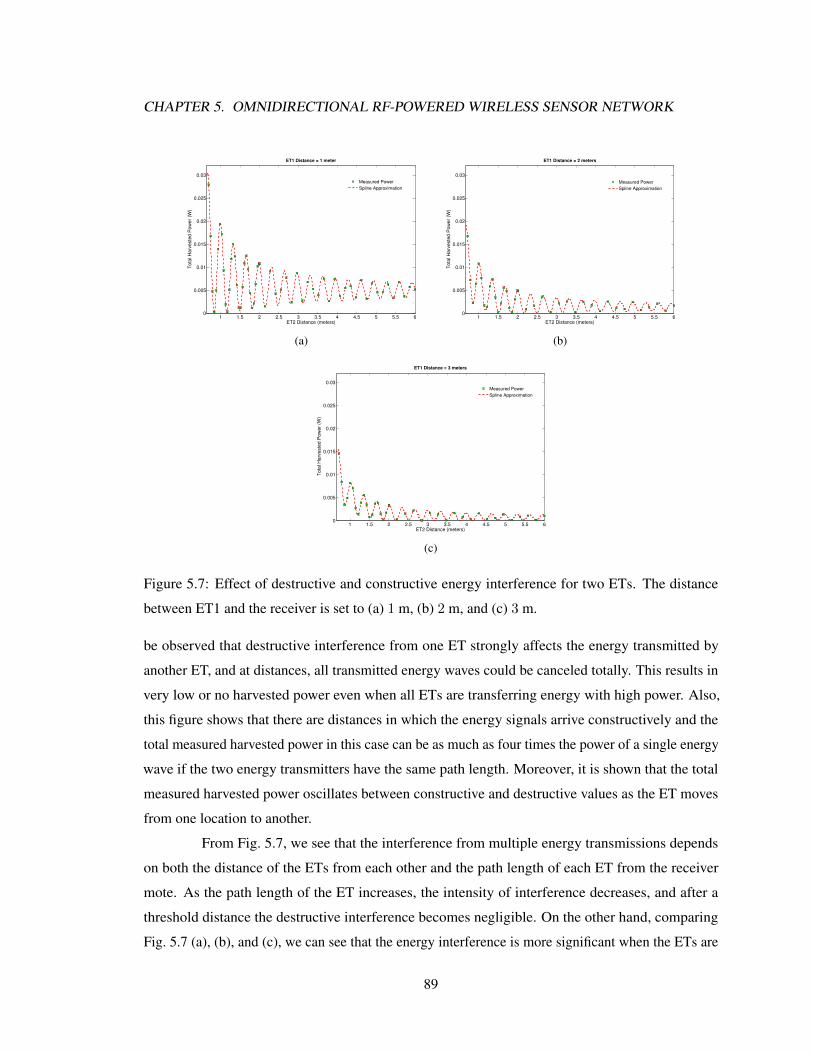
CHAPTER 5. OMNIDIRECTIONAL RF-POWERED WIRELESS SENSOR NETWORK
1 1.5 2 2.5 3 3.5 4 4.5 5 5.5 60
0.005
0.01
0.015
0.02
0.025
0.03
ET2 Distance (meters)
To
tal H
arv
este
d P
ow
er
(W)
ET1 Distance = 1 meter
Measured Power
Spline Approximation
(a)
1 1.5 2 2.5 3 3.5 4 4.5 5 5.5 60
0.005
0.01
0.015
0.02
0.025
0.03
ET2 Distance (meters)
To
tal H
arv
este
d P
ow
er
(W)
ET1 Distance = 2 meters
Measured Power
Spline Approximation
(b)
1 1.5 2 2.5 3 3.5 4 4.5 5 5.5 60
0.005
0.01
0.015
0.02
0.025
0.03
ET2 Distance (meters)
To
tal H
arv
este
d P
ow
er
(W)
ET1 Distance = 3 meters
Measured Power
Spline Approximation
(c)
Figure 5.7: Effect of destructive and constructive energy interference for two ETs. The distance
between ET1 and the receiver is set to (a) 1 m, (b) 2 m, and (c) 3 m.
be observed that destructive interference from one ET strongly affects the energy transmitted by
another ET, and at distances, all transmitted energy waves could be canceled totally. This results in
very low or no harvested power even when all ETs are transferring energy with high power. Also,
this figure shows that there are distances in which the energy signals arrive constructively and the
total measured harvested power in this case can be as much as four times the power of a single energy
wave if the two energy transmitters have the same path length. Moreover, it is shown that the total
measured harvested power oscillates between constructive and destructive values as the ET moves
from one location to another.
From Fig. 5.7, we see that the interference from multiple energy transmissions depends
on both the distance of the ETs from each other and the path length of each ET from the receiver
mote. As the path length of the ET increases, the intensity of interference decreases, and after a
threshold distance the destructive interference becomes negligible. On the other hand, comparing
Fig. 5.7 (a), (b), and (c), we can see that the energy interference is more significant when the ETs are
89

CHAPTER 5. OMNIDIRECTIONAL RF-POWERED WIRELESS SENSOR NETWORK
closer to the receiver. For example, the energy interference is higher when ET1 is 2 m away from
the mote compared to when it is 3 m away. It is lower compared to when ET1 is 1 m away. Thus,
interestingly, even though the ETs that are closer to the receiver provide higher levels of energy, they
can result in higher levels of energy cancellation. This shows the importance of energy interference
in the design of network protocols for RF-powered WSNs with multiple ETs.
The destructive and constructive interference of two incident energy waves are less pro-
nounced when the power of one wave dominates the other, or when the power of both waves are very
low. Let R1 and R2 denote the distances of ET1 and ET2 from the receiver mote, respectively. Based
on our experimental results, we define the energy cancellation range as the minimum path length
difference of the two ETs ∆Rmin with respect to the ET closer to the receiver and such that for all
values of R1 and R2 for which |R2 −R1| ≥ ∆Rmin the joint energy interference has negligible
effect on the amount of the total harvested power. The energy cancellation range could be useful in
the design of routing protocols, for managing energy cancellation effects, and for channel assignment
algorithms. The energy cancellation range is determined as follows. From Fig. 5.7, we see that when
the first ET is located at distance 1 meter from the receiver, the effect of constructive and destructive
energy interference in terms of fluctuations in the harvested power would be significant till ET2 is 2
m from the receiver. The energy interference decreases as the distance between ETs and the receiver
increases, and the interference becomes negligible when ET2 is 5 m away. Accordingly, the energy
cancellation range when ET1 is 1 m away from the receiver is found to be 4 meters. Similarly, the
energy cancellation range when ET1 is to 2 and 3 meters away is be found to be 0 m, when ET2 is 2
m away, and 1.5 m when ET2 is 1.5 m away, respectively.
5.2.5 Concurrent Energy Transmissions: Multi-Frequency
In this section, we show the feasibility and efficiency of RF energy harvesting at multiple
frequencies (multi-band RF harvesting).
Fig. 5.8a and 5.8b show the harvesting efficiency of the P2110 and P1110 energy har-
vesters [160] over the full ISM frequency range for 902 MHz to 928 MHz, for various ET-to-harvester
distances. These results are obtained from the powercast RF harvester data-sheets as well as the pow-
ercast wireless charging calculator [160] that contains the RF-to-DC conversion efficiency at different
frequencies and input powers. We can see that the efficiency of RF energy harvesting depends on the
input power, which is a function of the distance between the ET and the RF harvester. Moreover,
both pictures in Fig. 5.8 show that the design of the harvesting circuit has a significant impact on the
90

CHAPTER 5. OMNIDIRECTIONAL RF-POWERED WIRELESS SENSOR NETWORK
0
20
40
60
80
100
900 905 910 915 920 925 930
RF
-DC
Co
nve
rsio
n E
ffic
ien
cy %
Frequency (MHz)
ET distance= 1mET distance= 2mET distance= 3mET distance= 4mET distance= 5m
(a)
0
20
40
60
80
100
900 905 910 915 920 925 930
RF
-DC
Co
nve
rsio
n E
ffic
ien
cy %
Frequency (MHz)
ET distance= 1mET distance= 2mET distance= 3mET distance= 4mET distance= 5m
(b)
Figure 5.8: RF harvesting efficiency between the RF harvester and the ET for Powercast P2110 (a)
and P1110 (b) harvesting boards.
efficiency of harvesting. Specifically, the P2110 powerharvester outperforms the P1110 harvesting
board over long charging distances, while the P1110 harvesting board has better performance over
short charging distances. Most important, at each distance the RF energy harvesting circuit provides
almost the same performance and efficiency over a range of frequencies. As the bandwidth of the
energy signal is relatively small (i.e., 99% of the occupied bandwidth is approximately 63 kHz [161]),
our results demonstrate that if the RF harvester is optimized for a frequency range transferring energy
at different frequencies will not decrease the amount of harvested power when using multiple ETs,
independent of the distance between the energy transmitters and the receivers. Consequently, the RF
harvester can simultaneously and effectively harvest RF power over a range of different frequencies
within the bandwidth of its harvesting circuit.
91

CHAPTER 5. OMNIDIRECTIONAL RF-POWERED WIRELESS SENSOR NETWORK
5.3 Surviving Wireless Energy Interference
Recent advancements in energy harvesting and wireless energy transfer through radio
frequency (RF) waves have opened up new possibilities for powering the nodes of a wireless sensor
network (WSN) wirelessly. This not only extends the network lifetime, but also obviates the problem
of retrieving sensors and physically replacing batteries. The RF energy harvesting sensors convert
the energy contained in incident electromagnetic radiation emitted by wireless energy transmitters
(ETs) into stored electrical charge within a capacitor or re-chargeable battery. This limited stored
energy can then be used for sensing, processing and communication. However, the high power of RF
waves emitted from ETs interfere with low-power data communications among sensor nodes. This
leads to interference and packet loss. The objective of this experimental study is to quantify this loss
under various placements of ETs, including choice of frequencies and separation distances.
Motivation. The Federal Communications Commission (FCC) permits up to 4 Watts effective
isotropic radiated power (EIRP) for wireless energy transfer. Most Commercial Off-The-Shelf
(COTS) ETs (e.g., Powercaster [160]) generate 3 Watts energy waves. These high levels of radiation
are much higher than those of typical sensors, such as the MicaZ, whose maximum transmission
power is limited to 1mW. Thus, the adverse impact of continuous RF energy transfer on sensor
communication should be quantified. One approach could be using duty-cycle based energy and
data transfer, resulting in controlled and pre-decided trade-offs between data throughput and energy
harvesting levels [138]. At the hardware level, the state-of-the-art RF energy harvesting circuits can
operate over a range of frequencies [162, 163]. Thus, if the ET frequencies can be separated from data
frequencies then the packet losses caused by simultaneous data and energy transfer may be minimized.
Previous empirical studies in WSNs have focused on understanding the coexistence between WSNs
and WiFi [154, 155], microwave ovens [156], and smart grids [157]. There are also experimental
studies on concurrent data transmissions on low-power wireless links [152, 151]. However, none
of them have studied the interference issues in WSNs with wireless energy transfer. Moreover, the
power difference between interfered signals (i.e. high power energy signal and low-power data) in
RF-harvesting sensor networks is much higher than those in the previous studies, which necessitates
to study the adjacent-channel interference of energy signals on low-power data communications in
practice. To fill these gaps, this study is looking to find what are the observable impacts of energy
interference, how to survive such interference, and leverage the interference level at each node for
reliable data and energy transfer.
Experimental methodology. We conduct a series of experiments at indoor and outdoor locations to
92

CHAPTER 5. OMNIDIRECTIONAL RF-POWERED WIRELESS SENSOR NETWORK
study the effects of (i) RF energy interference on data communication, (ii) the benefits of energy
transfer when spread over different frequencies (i.e., under various separation levels of energy and
data frequencies), and (iii) the location of ETs on packet delivery. We present the distributions of
energy interference measured by sensor nodes for different energy frequencies. Our experiments
involve both statistical and time-trace measurements of packet reception rates, as well as the received
interferer power under carefully-designed conditions. We use Mica2 motes and RF frequency-tunable
ETs. To the best of our knowledge, this is the first empirical study on RF energy harvesting sensor
networks.
Summary of findings. Our measurements indicate the presence of hard separation thresholds in the
frequency domain that guarantee successful data packet reception among sensor nodes when ETs are
transferring energy. This threshold changes with indoor/outdoor locations and separation distance
of the ETs from the sensors. We identify three regions based on the separation of the energy and
data transfer channels on the frequency scale, which we name as black, gray, and white, with high,
moderate and low packet error rates, respectively.For example, the packet reception rate (PRR) when
the ET transfers energy in the gray region can vary significantly with high temporal fluctuations.
Also, sensors do not receive any packets in the black frequency region. However, wireless energy
transfer at any white band of frequencies result in higher than 90% PRR. We find differing behavior
in indoor and outdoor environments. For example, when RF transfer is done in the gray frequencies
with increasing ET distance outdoor, the PRR improves monotonically. However, in indoor spaces,
as ET increases, PRR has fluctuations due to signal reflections. On the contrary, when ET transfers at
white frequencies, the PRR is almost the same in both indoor and outdoor experiments, regardless of
ET locations. Finally, we find the interferer power at the sensor node that can be used to detect the
frequency regions and set the appropriate energy transfer frequencies of ETs.
The rest of the part is organized as follows. In Section 5.3.1 we describe our experimental
methodology. Section 5.3.2 presents measurement results on packet reception performance, including
the effect of multifrequency wireless energy transfer and the placement of the ET. Results on the
distribution of received energy interference are discussed in Section 5.3.3. Section 5.3.4 presents the
temporal variability of the energy interferer power.
93

CHAPTER 5. OMNIDIRECTIONAL RF-POWERED WIRELESS SENSOR NETWORK
5.3.1 Experimental Platform and Methodology
5.3.1.1 Hardware and software
We use Mica2 motes as the data communicating and energy harvesting nodes. Each mote is
equipped with CC1000 radio operating at 915 MHz with a default RF transmission power of 0 dBm.
The receiving sensitivity is −98 dBm. The CC1000 radio supports the measurements of the received
signal strength (RSSI). We link the P2110 RF energy harvesters from Powercast Co. [160] to the mote.
The RF frequency-tunable wireless ET is an Agilent N5181 MXG RF signal generator connected to
an amplifier with a 50 Ω omnidirectional antenna and 3 W output power in the 902–928 MHz band.
This configurable ET setup lets us change the frequency of wireless energy transfer precisely.
5.3.1.2 Measurement Metrics
We use interference power and PRR as the measurement metrics. The PRR is the fraction
of packets that are received within a time window over the total transmitted packets. We use a total
of 360 packet transmission epochs to estimate the PRR with a precision of 1.2% for each particular
combination of energy transmission frequency and distance between the ET and the motes. For
each ET energy frequency, the motes take 600 RSSI samples at the rate of 10 samples/sec over the
data channel (i.e., 915 MHz) that is important in a node’s point of view. Six hundred RSSI samples
are enough to collect meaningful measurements about the level of energy interference on the data
channel.
5.3.1.3 Locations
We conduct our experiments in indoor and outdoor environments. For the indoor environ-
ment we select a space with four plain walls and no other intermediate reflective objects to limit
time-varying changes in the wireless channel due to multi-path fading and shadowing. The second
set of measurements are conducted in an open-space outdoor, with no structural obstructions. Each
experiment involves three nodes: The sender, the receiver, and the wireless ET. The motes and ET
are placed on a flat table, 0.5 m from the floor. The sender and receiver nodes are placed one meter
from each other, and they are equidistant from the ET. The locations of the sender and receiver sensor
nodes are fixed, but we vary the frequency and distance of the ET and measure the packet reception
rate and the relative interference experienced by the sensor motes.
94

CHAPTER 5. OMNIDIRECTIONAL RF-POWERED WIRELESS SENSOR NETWORK
0
20
40
60
80
100
911 912 913 914 915 916 917 918 919
Ave
rag
e P
acke
t R
ece
ptio
n R
ate
(P
RR
)
Energy Frequency (MHz)
indoor
Distance ET = 1mDistance ET = 3mDistance ET = 5m
(a) Indoor scenario
0
20
40
60
80
100
911 912 913 914 915 916 917 918 919
Ave
rag
e P
acke
t R
ece
ptio
n R
ate
(P
RR
)
Energy Frequency (MHz)
outdoor
Distance ET = 1mDistance ET = 3mDistance ET = 5m
(b) Outdoor scenario
Figure 5.9: Effects of varying wireless ET frequencies on PRR (a) indoor and (b) outdoor.
20
40
60
80
100
1 2 3 4 5
Ave
rag
e P
acke
t R
ece
ptio
n R
ate
ET Distance (meters)
Gray Frequency = 913.600MHzGray Frequency = 916.400MHz
White Frequency = 918.200MHzBlack Frequency = 915,600MHz
(a) Indoor scenario
20
40
60
80
100
1 2 3 4 5
Ave
rag
e P
acke
t R
ece
ptio
n R
ate
ET Distance (meters)
Gray Frequency = 913.600MHzGray Frequency = 916.400MHz
White Frequency = 918.200MHzBlack Frequency = 915,600MHz
(b) Outdoor scenario
Figure 5.10: Effects of ET distance on the PRR at gray, white, and black energy frequencies (a)
indoor and (b) outdoor.
5.3.2 Packet Reception Rate
When the strength of data signal is sufficiently above the noise and interference data
packets can be successfully received and decoded. However, as the transmission power of the RF
waves is significantly higher and because the power contained in the energy signal may leak into
adjacent data communication channel, interference and packet losses may occur if this transfer occurs
at different frequencies.
• PRR and frequency. Figures 5.9a and 5.9b present the average PRR as a function of varying ET
frequencies indoor and outdoor, respectively. The data communication frequency is centered at 915
MHz. The experiments show that three distinct regions occur: In the middle region of the graph,
95

CHAPTER 5. OMNIDIRECTIONAL RF-POWERED WIRELESS SENSOR NETWORK
there is the band of black frequencies, in which none of the packets that are transferred between
sensor motes are successfully received. In these black frequencies, the power of energy signals that
leaks into the data channel is high enough to completely block all data communications. We observe
that the actual frequency range of black region depends on the distance of ET from the receiver
(Fig. 5.9). More specifically, the spread of the black frequency region for the ET with distance of
1m is 2 MHz; for the ET with distance 3m is 1.2 MHz. Similarly, for the ET with distance 5m it is
0.8 MHz. Fig. 5.9 shows that even when the ET is 5m away from the mote, which is the maximum
effective charging range in our testbed, there are still energy frequencies with 100% packet loss.
Thus, an appropriate separation of energy and data channels must be chosen in the design of protocols
for such RF powered nodes.
On the extreme ends of the plots there are two frequency regions where the PRR is always
uniformly high. We call these regions white areas, where the sensor motes experience correct
reception even in the presence of concurrent wireless energy transfer from the ET. We observed that
the white range for indoor environment includes all energy frequencies higher than 917.600 MHz and
lower than 912.200 MHz (Fig. 5.9a). As shown in Fig. 5.9b, the white outdoor range includes those
frequencies that are higher than 917.800 MHz and lower than 912 MHz. ET placement does not
appear to affect the extent of the white region. These results further show that frequency separation
is a better approach for sensor survival of energy interference and to boost network throughput,
compared to duty-cycle based approaches.
Finally, we observe that both indoor and outdoor there are frequency ranges where the
PRR is rather unstable. These energy frequency regions are the gray areas. In these, the motes
experience variations in PRR ranging from 50% to 90%. While the high power of energy transfer
at gray frequencies still leaks into the data channel, the energy interference has a power that
is nearly the one of the data signal at the receiver. The pattern of fluctuations depends on the
environment and on the form of energy signal. Interestingly, we observed that outdoor the patterns
of fluctuations are symmetric for different ET distances. Indoor, however, even when multi-path
fading and shadowing are limited, the reflections due to the walls resulted in different constructive
and destructive interference levels at the receiver. As a consequence, for indoor environments we
observe asymmetric variations of packet reception with varying ET distances. Furthermore, our
measurements show that the spread of the gray region in both indoor and outdoor depends on the
location of ETs. In particular, as the distance of ET increases, the width of the gray region also
increases: When the ET is 1m away, the gray region is the narrowest; when the ET is 5m away, it is
the widest.
96

CHAPTER 5. OMNIDIRECTIONAL RF-POWERED WIRELESS SENSOR NETWORK
0
0.2
0.4
0.6
0.8
1
-90 -80 -70 -60 -50
No
rma
lize
d F
req
un
cy
Received Energy Interferer Power (dBm)
Gray Region
ET Frequency = 917,600ET Frequency = 916,200ET Frequency = 913,600ET Frequency = 912,600ET Frequency = 912,200
Data SignalAmbient Noise
(a)
0
0.2
0.4
0.6
0.8
1
-90 -80 -70 -60 -50
No
rma
lize
d F
req
un
cy
Received Energy Interferer Power (dBm)
White and Black Regions
ET Frequency = 915,600ET Frequency = 915,200ET Frequency = 914,600ET Frequency = 914,200ET Frequency = 911,800
ET Frequency = 918ET Frequency = 918,200
Data SignalAmbient Noise
(b)
Figure 5.11: Distribution of RSSI for energy interference indoor for varying ET frequencies in gray,
white, and black regions.
• PRR and distance. Fig. 5.10 compares the PRR for five different ET distances for a mix of gray,
black, and white frequency regions, both indoor and outdoor. First, we observe that the energy
frequency of 915.6 MHz is within the black area when the ET is 1, 2, and 3 m away from the motes.
As the distance increases (4 and 5 m), this frequency moves to the gray area. This observation
highlights the importance of ET location in RF transfer frequencies assignment. We also observed
that the indoor PRR at the gray frequencies does not improve monotonically for increasing distances
of the ET. This is because of small reflections of energy signals. For example, at the gray frequency
of 913.600 MHz, the PRR is lower when ET is 3 m away that when it is 2 m away. Outdoor, instead,
packet reception improves monotonically with increasing distances of the ET.
Overall, our experimental study reveals that the existence and width of the three regions
has important implications for RF energy harvesting-based WSNs. In particular, we have observed
that the frequency of energy and data signals need to be separated beyond a threshold that depends
on the distance of the ET from the nodes to allow packets to be received successfully. The naming
for white, gray, and the white areas is inspired from earlier works observing similar behaviors for
classical sensor networks [9], which are concerned only on inter-nodal spatial distance. In this work,
the demonstrated areas refer to frequency domain in RF energy harvesting sensor networks.
5.3.3 Energy Interference
In traditional WSNs, the RSSI provides an indication of connectivity, aids access points
selection, and is used to determine error-prone wireless links. However, it is not immediately obvious
97

CHAPTER 5. OMNIDIRECTIONAL RF-POWERED WIRELESS SENSOR NETWORK
0
0.2
0.4
0.6
0.8
1
-90 -80 -70 -60 -50
No
rma
lize
d F
req
un
cy
Received Energy Interferer Power (dBm)
Gray Region
ET Frequency = 917,600ET Frequency = 916,200ET Frequency = 913,600ET Frequency = 912,600ET Frequency = 912,200
Data SignalAmbient Noise
(a)
0
0.2
0.4
0.6
0.8
1
-90 -80 -70 -60 -50
No
rma
lize
d F
req
un
cy
Received Energy Interferer Power (dBm)
White anf Black Region
ET Frequency = 915,600ET Frequency = 915,200ET Frequency = 914,600ET Frequency = 914,200ET Frequency = 911,800
ET Frequency = 918ET Frequency = 918,200
Data SignalAmbient Noise
(b)
Figure 5.12: Distribution of RSSI for energy interference outdoor for varying ET frequencies in gray,
white, and black regions.
how the interferer power measured by the sensor nodes could be used to determine the energy
frequency regions and preferred power transfer frequencies in RF harvesting WSNs. In this section,
we aim at studying how knowing the distributions of the energy interference strength can be used
by a node to detect in which region (white, gray or black) is the node, and the appropriate energy
transfer channels it can use.
• RSSI distributions with frequency. Figures 5.11 and 5.12 illustrate the impact of different energy
frequency regions on the distribution of the received interferer power indoor and outdoor, respectively.
The y-axis corresponds to the RSSI values in dBm measured by the CC1000 radio of the Mica2 mote.
The distance between the ET and the motes is 1 m. We also present the signal strength distribution of
the ambient noise and of the data signal both indoor and outdoor, measured in absence of energy
transfer. The rightmost distribution shows the RSSI of data signal (around −49 dBm), and the
leftmost one shows the measured ambient signal distribution (between −93 dBm and −89 dBm)
indoor. The outdoor noise is between 91 dBm and −75 dBm. Figures 5.11 and 5.12 show that the
RSSI of the recorded energy can be clustered into three classes corresponding to three different
frequency areas. We observe a correlation between the frequency separation of energy and data
and the clusters. However, within each cluster this correlation does not necessarily hold. The RSSI
distributions of black regions are close to each other and can be clustered with the data signal, while
the distributions of white region can be clustered with the ambient noise. The cluster for the gray
region is in the middle. We notice that the gray area exhibits a wider range of RSSI than that of the
other two regions.
The range of the interferer signal strength for the gray region vary from −87 dBm to
98

CHAPTER 5. OMNIDIRECTIONAL RF-POWERED WIRELESS SENSOR NETWORK
Outdoor Indoor
ET FrequencyMean
RSSIStdV PRR
Mean
RSSIStdV PRR
918,200 -87.069 0.010 98% -88.534 0.011 100%
918,00 -86.683 0.012 94% -89.444 0.012 100%
917,600 -78.476 0.010 86% -88.534 0.011 100%
916,200 -65.785 0.006 47% -67.737 0.009 42%
915,600 -54.283 0.001 0% -55.219 0.001 0%
915,200 -48.550 0.001 0% -49.187 0.001 0%
914,600 -55.607 0.001 0% -55.953 0.001 0%
914,200 -61.602 0.001 0% -59.236 0.001 0%
913,600 -79.864 0.010 87% -75.355 0.005 75%
912,600 -85.364 0.009 97% -79.872 0.008 83%
912,200 -79.472 0.022 92% -86.414 0.010 100%
911,800 -87.617 0.011 100% -91.473 0.010 100%
Table 5.3: Map of energy interference power and associated PRR.
−65 dBm indoor, and from −84 dBm to −64 dBm outdoor. In this region, the RSSI samples are
normally distributed and can be categorized into three groups: High, medium, and low. The first
group includes ET frequencies such as 916.200 MHz that exhibits higher RSSI, and hence lower
packet reception rates. The second group contains frequencies such as 913.600 MHz indoor and
as 912.200 MHz outdoor showing slightly lower RSSI. Finally, the third group in the gray area
corresponds to ET frequencies with negligible energy interference.
The recorded RSSI at each energy transfer frequency within the gray area have different
variances. Some ET frequencies can cause higher variations of RSSI (i.e., 912.200 MHz outdoor),
while frequencies like 913.600 MHz have low RSSI variations. Comparing the two figures, we
find that the RSSI values in the gray area exhibits markedly different patterns indoor and outdoor.
For example, the indoor ET frequency 912.600 MHz has higher interferer power compared to
917.600 MHz. These power values are lower outdoor. It is shown that the black frequency range
(rightmost point of the plots) shows a large spike of received power both indoor and outdoor, but the
interference patterns remain the same. The RSSI distributions reveal that the energy interference at
the white frequencies in both indoor and outdoor environments are negligible. This confirms the high
values of PRR shown in Section 5.3.2.
99

CHAPTER 5. OMNIDIRECTIONAL RF-POWERED WIRELESS SENSOR NETWORK
0
5
10
15
20
25
30
35
40
45
50
-82 -80 -78 -76 -74 -72 -70 -68 -66
Fre
qu
ncy
Received Energy Interferer Power (dBm)
ET Distance = 1mET Distance = 3mET Distance = 5m
(a)
0
5
10
15
20
25
30
35
40
45
-90 -88 -86 -84 -82 -80 -78 -76
Fre
qu
ncy
Received Energy Interferer Power (dBm)
ET Distance = 1mET Distance = 3mET Distance = 5m
(b)
0
5
10
15
20
25
30
35
40
45
50
-94 -92 -90 -88 -86 -84 -82 -80
Fre
qu
ncy
Received Energy Interferer Power (dBm)
ET Distance = 1mET Distance = 3mET Distance = 5m
(c)
Figure 5.13: Effects of different ET distances on distributions of energy interference for (a) indoor
gray region, (b) outdoor gray region, and (c) outdoor white region.
Table 5.3 summarizes the energy interference power and associated PRR for different ET
frequencies from all regions in both indoor and outdoor environments, and strongly suggests that the
measurement of energy interference within the sensor node can be used as a good estimate to detect
energy areas and appropriate energy frequencies in RF harvesting sensor networks.
• RSSI and distance. We investigate the relationship between the distance among ET and motes,
and the RSSI at the receiving mote. We plot the received interferer power for varying distances and
energy frequency regions both indoor and outdoor. Due to space limitations, we show results for
the gray frequency (913.600 MHz) indoor (Fig. 5.13a) and outdoor, and for the white frequency
(911.800 MHz) regions outdoor only (Fig. 5.13b).
In Figure 5.13a, we see that the interference may increase with increasing ET distance.
Specifically, the measured RSSI for ET located at distance 1m is about -76 dBm, however, the RSSI
increases to about -74 dBm at distance 3m. This occurs because of reflections in the indoor setup,
and confirms the asymmetric PRR variations over different ET distances. In outdoor environment,
the received interferer power decreases as the distance of ET increases. In particular, Figure 5.13b
shows that the measured power is about -80 dBm for ET distance 1m, and it decreases to about
-84 dBm and -87 dBm for ET distances 3m and 5m, respectively. Thus, the distribution of energy
interference at the white frequency region has very few changes with the location of the ET. Our
measurements indicate that both gray and white frequencies have normal interference distributions
over all ET distances.
100

CHAPTER 5. OMNIDIRECTIONAL RF-POWERED WIRELESS SENSOR NETWORK
-90
-85
-80
-75
-70
-65
-60
0 100 200 300 400 500 600
Re
ce
ive
d I
nte
rfe
ren
ce
Po
we
r (d
Bm
)
Sample #
Gray Region
Ambient NoiseET Distance = 1mET Distance = 3mET Distance = 5m
(a)
-90
-85
-80
-75
-70
-65
-60
0 100 200 300 400 500 600
Re
ce
ive
d I
nte
rfe
ren
ce
Po
we
r (d
Bm
)
Sample #
Gray Region
Ambient NoiseET Distance = 1mET Distance = 3mET Distance = 5m
(b)
-90
-85
-80
-75
-70
-65
-60
0 100 200 300 400 500 600
Re
ce
ive
d I
nte
rfe
ren
ce
Po
we
r (d
Bm
)
Sample #
White Region
Ambient NoiseET Distance = 1mET Distance = 3mET Distance = 5m
(c)
-90
-85
-80
-75
-70
-65
-60
0 100 200 300 400 500 600
Re
ce
ive
d I
nte
rfe
ren
ce
Po
we
r (d
Bm
)
Sample #
White Region
Ambient NoiseET Distance = 1mET Distance = 3mET Distance = 5m
(d)
-90
-85
-80
-75
-70
-65
-60
-55
-50
-45
0 100 200 300 400 500 600
Re
ce
ive
d I
nte
rfe
ren
ce
Po
we
r (d
Bm
)
Sample #
Black Region
Ambient NoiseET Distance = 1mET Distance = 3mET Distance = 5m
(e)
-90
-85
-80
-75
-70
-65
-60
-55
-50
-45
0 100 200 300 400 500 600
Re
ce
ive
d I
nte
rfe
ren
ce
Po
we
r (d
Bm
)
Sample #
Black Region
Ambient NoiseET Distance = 1mET Distance = 3mET Distance = 5m
(f)
Figure 5.14: Temporal characteristics of energy interference power in indoor (a, c, e) and outdoor (b,
d, f) environments for gray, black, and white frequency regions.
5.3.4 Temporal Change in Energy Interference
In this section, we examine how the energy interference varies with time for indoor and
outdoor environments.
Figure 5.14 shows the received energy interferer power for the three colored frequency
regions at different ET distances of 1m, 3m, and 5m. The energy interference when ET transfers at
the gray frequency region shows significant variations over time in the outdoor environment. On the
other hand, the indoor scenario that caused noticeable variations in RSSI compared to the ambient
noise, exhibits comparatively less temporal variation. The high temporal variation results indicate
not only sensor nodes experience variable PRR over different gray frequencies, but also the fact
that nodes experience time varying energy interference at each frequency. In addition, these results
suggest to continuously measure the energy interferer power at gray frequencies since the RSSI
can vary significantly over time. Figures 5.14c and 5.14d show the temporal variations in the white
101

CHAPTER 5. OMNIDIRECTIONAL RF-POWERED WIRELESS SENSOR NETWORK
region, which is comparatively less than those in the gray region. The interference caused by energy
transfer in the black frequency band caused no variations in the measured RSSI. Interestingly, in all
the plots, we find that the variation of the interferer power decreases as the distance between ET and
the sensor node increases.
5.4 Energy Models and Analysis
Electromagnetic waves carry energy in the form of electric and magnetic fields, which
can be converted (with some losses) and stored as energy at the receiving front-end, and used to
power the processing and communication circuits of the nodes of a wireless sensor network (WSN).
The ability of transferring energy via contact-less radio frequency (RF) will ensure the sensor nodes
to remain operational for long times, without the need of costly battery replacement efforts [138].
Current prototypes of RF transfer, however, have limited charging range (few meters) and efficiency
(40 to 60%). This imposes the concurrent and coordinated use of multiple ETs to power an entire
WSN [164].
While multiple ETs are needed to ensure high energy transfer rates, they introduce inter-
ference among RF waves from different ETs, leading to significant and various constructive and
destructive combinations over the network deployment area. Being able to compute the energy
harvestable at a given point in space is a non-trivial task, as it depends on the relative locations
of active ETs, path loss information, and on the different distances from the ETs and a receiver at
that point. However, estimating the harvestable energy is a key first step in network planning and
protocol design for long-lived WSNs. For example, at the link layer, sensors placed in regions that
will receive energy at low transfer rates should have lower duty cycles. At the network layer, routes
can be pre-computed to pass through regions with high energy transfers. Task assignment, at the
application layer can also be facilitate by knowing how much energy will be available at a node
at a certain time. Deriving closed form expressions of the energy harvestable at any point in the
deployment space of the WSN is the main aim and contribution of this section.
Our approach starts from considering the path-loss models between one transmitter and
one receiver, such as the one expressed by the Friis transmission equation [165, 166] estimating
the received power between two nodes. We then incorporate in these models results from array
factor calculation in an N-element antenna array and phased array [167, 168, 169] used to estimate
the cumulative contribution of all the isotropic radiating elements at any far-field point. Hardware
design factors, such as the diode operational parameters used in voltage multiplier sections of the
102

CHAPTER 5. OMNIDIRECTIONAL RF-POWERED WIRELESS SENSOR NETWORK
energy harvesting circuit and RF-to-DC conversion efficiency, are integrated in our communication-
centric analytical models. The resulting closed matrix form expressions give an estimate of the
harvestable energy from multiple wireless ETs at any point, explicitly considering the unique features
of constructive and destructive combination of RF waves. Our analytical approach first concentrates
on the case of two and N ETs in the plane, and then generalizes the results to N ETs in 3D.
Through our derived models we analyze and determine optimal distributions of power outage, energy
interference, and harvested voltage and power over the whole WSN. Our analysis shows that the
received power from multiple ETs over the entire network and the network energy interference
caused by concurrent RF energy transfer has Log-Normal distributions. In addition, the harvested
voltage over the whole WSN has Raleigh distribution due to use of either diodes or transistors, which
are typically used in energy harvesting circuits, and to their input power-voltage curves.
The rest of part is organized as follows. In Section 5.4.1 we determine the harvestable
energy in the plane. Section 5.4.2 extends generalize our findings to 3D spaces. In Section 5.4.3 we
study the impact of wireless energy interference from multiple ETs over the entire WSN, and present
the observed distributions of energy-related metrics.
5.4.1 2D RF Energy Model
In this section we develop analytical expressions for the total harvestable energy from two
ETs at any given location in the plane. We then extend these expressions to the case of N ETs in the
plane. The ETs and sensors are assumed to be equipped with omnidirectional dipole antennas, and
ETs transfer RF waves with the same initial phase. The RF waves carry energy in the form of the
electric field. Computation of the intensity of harvestable power from two ETs starts with computing
the sum of their electric fields at any given location. The electric field (E) from an ET measured by a
receiver device at distance R is:
E =√Z0Se
−jkR =√Z0Se
−j( 2πλ
)R,
where Z0 is a physical constant indicates the wave-impedance of a plane wave in free
space [170]. Moreover, S is the power spatial density at distance R (i.e., the power per unit area),
and k is the wavenumber of the energy wave (i.e., the magnitude of the energy wave vector). The
term kR indicates the phase shift of the transmitted energy signal at distance R. Here, S = GtPt4πR2 ,
where Gt is the transmitter gain and Pt is the output power of the ET. Fig. 5.15 shows a scenario
with two ETs.
103

CHAPTER 5. OMNIDIRECTIONAL RF-POWERED WIRELESS SENSOR NETWORK
Figure 5.15: Two ETs transferring power on the same frequency to a receiver node at distance R1
and R2.
The total electric field ET at the receiver when both ETs are transmitting energy is merely
the superposition of their individual electric fields:
ET = E1 + E2 =√Z0S1e
−jkR1 +√Z0S2e
−jkR2 ,
where the first term is the electric field from ET1 and the second term is the electric field
from ET2. The magnitude of the field can be expressed as:
|ET | =√|E1|2 + |E2|2 + 2|E1||E2|cos(k(R2 −R1)).
Therefore, the density of the total transferred power at the receiver is:
ST =|ET |2
Z0= S1 + S2 + 2
√S1S2cos(k∆r),
where ∆r = |R1 − R2| is the difference of the distances between the two ETs and
the receiver. Since an ET is an isotropic radiator (an EM source radiating the same power in all
directions), the expression for the magnitude of E can be expanded as follows:
ST =G1P1
4πR21
+G2P2
4πR22
+2
4π
√P1P2G1G2
R21R
22
cos(k∆r),
where P1 and P2 are the transmission powers and G1 and G2 are the transmission gains of
ET1 and ET2, respectively.
104

CHAPTER 5. OMNIDIRECTIONAL RF-POWERED WIRELESS SENSOR NETWORK
corr =
1/R1 cos(k(R1 −R2))/R1 . . . cos(k(R1 −Rn))/R1
cos(k(R2 −R1))/R2 1/R2
......
. . .
cos(k(Rn −R1))/Rn . . . 1/Rn
(5.2)
The aperture of the antenna of the receiver determines how well it can harvest power from
an incoming EM wave. The total available power at an isotropic receiving antenna with an effective
area A is given by:
P rT = STA = STGr(λ2
4π
),
where Gr is the gain of the RF harvester antenna. The total received power from two ETs
would be as follows:
P rT = G1P1Gr( λ
4πR1
)2+G2P2Gr
( λ
4πR2
)2+2( λ
4π√R1R2
)2Gr√G1G2
√P1P2cos(k∆r).
If two energy transmitters have the same antenna gain (i.e., Gt) and transmission power
(i.e., Pt), then the total received energy at the receiver node simplifies to:
P rT = PtGtGr( λ
4π
)2( 1
R21
+1
R22
+2cos(k∆r)
R1R2
).
According to the RF wireless charging model, the amount of harvested power by the RF
energy harvesting receiver would be
PH = ηP rT ,
where η is the RF-to-DC conversion efficiency. This formula captures both destructive and
constructive interferences at any given location by considering the path lengths as well as the path
differences between the ETs and the receiver. The harvested voltage could be found by VH = F (P rT )
where the function F relates input power to harvested voltage and depends on the energy harvesting
circuit [1].
Similarly, we can obtain the total received power from N ETs as follows:
105

CHAPTER 5. OMNIDIRECTIONAL RF-POWERED WIRELESS SENSOR NETWORK
P rT =Gr( λ
4π
)2[ N∑i=1
PiGiR2i
+
N∑i=1i 6=j
N∑j=1
√GiGjPiPj
RiRjcos(k(∆rij))
],
where Pi and Gi are the transmission power and the transmission gain of ETi, respectively,
and Gr is the gain of the receiver antenna. If all ETs have the same antenna gain and transmission
powers, then the total received energy at the receiver node simplifies to:
P rT = PtGtGr( λ
4π
)2[ N∑i=1
1
R2i
+
N∑i=1i 6=j
N∑j=1
cos(k(∆rij))
RiRj
],
which in matrix form can be written as follows:
P rT =(P)(corr
)(R−1
)where P is a constant row vector with size N defined as
(PtGtGr(
λ4π )2
)·1T , the N ×N correlation
matrix corr is shown in Equation (5.2), and the distance matrix R−1 is:
R−1 =
1/R1
1/R2
...
1/Rn
5.4.2 3D RF Energy Model
In practice and for most applications of energy harvesting sensor network such as health-
care, structural health minoring, smart home, etc we need to deal with three-dimensions, where the
heights of ETs and sensor nodes are not necessary the same. Accordingly, in this section we first
we explain the coordinate system for computing transmitted power from an ET, and then we derive
the analytical model of harvestable energy for three-dimensional case of a sensor network with N
wireless energy transmitters.
Fig. 5.16 shows the geometrical parameters for finding the electric field of ETn with
respect to the phase reference at origin. We assume the receiver is located at a given point M,
(r,φ,θ), and it is a far-field point in regard to all energy transmitters. Here, ~ρn is the vector from the
106

CHAPTER 5. OMNIDIRECTIONAL RF-POWERED WIRELESS SENSOR NETWORK
Figure 5.16: Geometrical parameters of an ETn transferring wireless energy to a receiver at far-field
point M.
origin to the ETn (ET vector); ~r is the vector from origin to the observation point (energy transfer
direction vector), and ~Rn is the distance vector from the ET to the receiver. Moreover, using spherical
coordinates, x = r sin(θ) cos(φ), y = r sin(θ) sin(φ), and z = r cos(θ), respectively. For ETn, the
electric field at a far-field point, M, can be expressed as
En =√Z0Sne
−jk| ~Rn| =√Z0Sne
−jγn
where k = 2πλ is the wave number, and γn is the phase shift of emitted energy signal from ETn at
the receiver with respect to the origin, and Sn is the power density of transmitted signal at point M
and would be computed as
Sn =GnPn
4π| ~Rn|2sin2(θ)
whereGn) is the gain ofETn assuming its antenna is oriented to z direction andPn is the transmission
power. Using spherical coordinates, Rn for a far-field point M (i.e. r ρn) can be approximated as
follows:
~Rn = ~r − ~ρn
107

CHAPTER 5. OMNIDIRECTIONAL RF-POWERED WIRELESS SENSOR NETWORK
Figure 5.17: (a) Received power samples over the WSN space with 40 ETs. (b) Log-Normal
distributions of the network wide received power from multiple ETs. (c) Power outage probability
based on CDF of the received power from multiple ETs.
| ~Rn| = |~r| −~r · ~ρn|~r|
| ~Rn| = |~r| − | ~ρn| sin(θ) cos(φ− φn)
Thus, the electric field of ETn at the receiver located in point M would be found as
En = sin(θ)
√Z0GnPn
4πR2n
(e−jkrejkρn sin(θ) cos(φ−φn)
)We assume the location of N energy transmitters are given by ~ρ1, ~ρ2, ~ρ3, ..... , ~ρn. We
need to find the received and harvestable power at point M, determined by (r, φ, θ). Similar to the 2D
case, the total electric field strength at the receiver, when N ETs are transmitting simultaneously, is
the superposition of individual received electric fields. Hence, the density of total transferred power
at the receiver can be calculated as follows,
ST =|ET |2
Z0=
1
Z0
[ N∑n=1
|En|2 +N∑i=1i 6=j
N∑j=1
(|Ei||Ej | cos(γi − γj))],
where the relative phase difference of EM waves from ETi and ETj is found as :
108

CHAPTER 5. OMNIDIRECTIONAL RF-POWERED WIRELESS SENSOR NETWORK
P rT = sin2(θ)PtGtGr(λ
4π)2
[ N∑i=1
1
(r − ρi sin(θ) cos(φ− φi))2
+N∑i=1i 6=j
N∑j=1
cos(γi − γj)(r − ρi sin(θ) cos(φ− φi))(r − ρj sin(θ) cos(φ− φj))
], (5.2)
γi − γj = k(Ri −Rj
)= −k sin(θ)
[(ρi − cos(φ− φi)
)−
(ρj − cos(φ− φj)
)].
Thus, the available power at point M would be:
P rT = Grλ2
4πST = Gr
λ2
4π
[ N∑i=1
Si +
N∑i=1i6=j
N∑j=1
(√SiSj cos(γi − γj))
],
P rT = sin2(θ)Gr( λ
4π
)2[ N∑i=1
PiGiR2i
+N∑i=1i 6=j
N∑j=1
√GiGjPiPj
RiRjcos(γi − γj))
],
where Pi, Pj , and Gr are the transmission power of ETi, the transmission power of ETj ,
and the receiver gain, respectively. If ETs have the same antenna and transmission powers, then the
available power at the receiver node can be simplified to
P rT = sin2(θ)PtGtGr( λ
4π
)2[ N∑i=1
1
R2i
+
N∑i=1i 6=j
N∑j=1
cos(γi − γj)RiRj
],
which is equal to Equation (5.2). This can be written in matrix form as: P rT = (P )(corr)(R−1)
where the distance matrixR−1 is [1/R1, 1/R2, . . . , 1/Rn], the row vectorP is equal to(
sin2(θ)PtGtGr(λ4π )2
)·
1T , and the correlation matrix corr would be:
corr(i, j) = cos(γi − γj)/Ri
109

CHAPTER 5. OMNIDIRECTIONAL RF-POWERED WIRELESS SENSOR NETWORK
Finally, the amount of harvested power by the RF energy harvesting receiver would be:
PH = ηP rT
where η is the RF-to-DC conversion efficiency. Also, the harvested voltage could be found
by VH = F (P rT ) where function F , similar to 2D case, depends on the energy harvesting circuit.
5.4.3 Analysis and Simulation Results
In this section, we analyze the performance of wireless energy transfer over a sensor net-
work with multiple ETs. A variable number of ETs is randomly deployed in a 50× 50 m2 grid. Each
ET transfers RF energy at center frequency 915 MHz with Effective Isotropic Radiated Power (EIRP)
equal to 4 W, which is the maximum transmission power allowed by the Federal Communications
Commission (FCC) for omni-directional energy transfer. The transmission parameters of all ETs are
assumed to be identical. The parameters of the energy harvesting receiver are set according to our
dual-stage energy harvester [1] with linear antenna gain of 6 dBi. The energy transfer of multiple
ETs has been analyzed over the whole WSN. In particular, each time we have computed the received
and harvested power in all points (samples) in the WSN deployment space, and accordingly found
the network distributions of multiple wireless energy transfer. To this end, all sample points from
the mesh grid range [0, 50] are selected with interval 0.1. We assume two energy transfer scenarios.
In the first scenario all ETs transmit omni-directional RF power at the same frequency, while in
the second scenario (i.e., FDMA-like) each ET transmits power at a different frequency. This latter
scenario is used as the base case for multiple energy transfer without interference. We focus our
analysis on studying network-wide performance of concurrent wireless energy transfer in terms of
power outage probability, energy interference, and harvested power and voltage.
5.4.3.1 Power outage probability
First, we investigate the power outage probability in sensor network when ETs are trans-
mitting omni-directional RF signals. The power outage probability is defined as the probability that
the received power from multiple ETs at a destination in the network be less than a given threshold.
Fig. 5.17-a shows the received power over different samples in a network with 40 ETs. We see that
the constructive and destructive interference of energy waves lead to different values of received
energy at each destination. Figures 5.18 depict that the PDF and CDF distributions of received power
for different number of ETs, namely, 10, 20, 30 and 40. Fig. 5.17-b shows that the received power
110

CHAPTER 5. OMNIDIRECTIONAL RF-POWERED WIRELESS SENSOR NETWORK
Figure 5.18: (a) Comparison of received power with energy interference and without interference.
(b) Energy interference samples over the sensor network with 40 ETs. (c) Log-Normal distributions
of energy interference for multiple ETs.
over the network has Log-Normal distribution (Gaussian distribution in a logarithmic scale such as
dBm). Also, Fig. 5.17-c indicates the effects of increasing ETs on the the received power over the
network. Interestingly, the probability that the received power from multiple ETs becomes larger
than 0 dBm is 20% for 10 ETs, 40% for 20 ETs, 60% for 30 ETs, and 70% for 40 ETs. In addition,
Fig. 5.17-c represents the outage probability when multiple ETs transmitting at the same frequency.
For example, when the minimum desired energy to power a sensor node is set to −5 dBm, then the
power outage probability is 50% for 10 ETs, 30% for 20 ETs, 15% for 30 ETs, and 10% for 40 ETs.
Furthermore, the outage probability does not exhibit linear dependency with the number of ETs.
Particularly, as the number of ETs increases, the rate at which the energy received changes does not
increase at the same rate.
5.4.3.2 Energy interference
Next, we study the distributions of energy interference due to concurrent energy transfer
from multiple ETs. To this end, we use FDMA transfer scheme as the base case for our comparisons,
in which ETs transmit power at different frequencies and there is no interference between simultane-
ous energy waves. The different between the received energy from ETs in the same band and ETs
transmitting with FDMA scheme is considered as the energy interference. Fig. 5.18-a compares the
received power over the network with 40 ETs. It is shown that the received power in the multi-energy
transfer at the same frequency could be at times greater, and at other times, smaller than FDMA. In
fact, at some points over network, we see higher energy while other points receive less energy than
111

CHAPTER 5. OMNIDIRECTIONAL RF-POWERED WIRELESS SENSOR NETWORK
Figure 5.19: (a) Dual-stage distributions of the harvested power (dBm) over the sensor network with
different number of ETs. (b) Rayleigh distributions of the harvested voltage over the network. (c)
CDFs of the harvested voltage over the network.
FDMA. Furthermore, Fig. 5.18-b shows interference in a network with 40 ETs. We see that energy
interference varies over the networks from locations with very high interference to ones with near
zero interference. Finally, Fig. 5.18-c depicts the distribution of energy interference for different
number of ETs 10, 20, 30, and 40. Interestingly, it is shown that energy interference over network
has Log-Normal distribution (Gaussian distribution in dBm scale).
5.4.3.3 Harvested voltage and power
We next investigate the distributions of the harvested power and voltage over the sensor
network. As shown in our previous work [1], regardless of the type of energy harvesting circuit, the
output voltage vs. input power (dBm) plot has an exponential curve due to use of either diodes or
transistors in voltage multiplier sections of the energy harvesting circuit. Moreover, the efficiency
curve (i.e. output power in dBm vs. input power in dBm) has polynomial distribution. In this section,
without loss of generality we emulate a dual-stage circuit which adaptively switches in low-power
and high-power regions based on our energy harvesting circuit prototype presented in [1].
Figures 5.19-a and 5.19-b show the PDF of the harvested power and harvested voltage over
the whole sensor network for 10, 20, 30, and 40 ETs. Importantly, it is shown that harvested voltage
over network has Rayleigh distribution, and harvested power clearly shows a dual-stage behavior
in its distribution. Fig. 5.19-c shows the CDF of harvested voltage in the network. We see that the
probability that the harvested voltage is less than 5V is 50% for 10 ETs, 25% for 20 ETs, 20% for 30
112

CHAPTER 5. OMNIDIRECTIONAL RF-POWERED WIRELESS SENSOR NETWORK
Figure 5.20: Intensity and patterns of harvested voltage.
ETs, and 15% for 40 ETs. Finally, Fig. 5.20 shows the harvested voltage map for 3 and 5 randomly
deployed ETs, when the dual-stage harvesting circuit is used. The circles, which also have the highest
harvested voltages, indicate the location of actual ETs. This figure depicts the randomness of energy
patterns over the network, and shows as the number of ETs increases the randomness of energy
patterns increases too. It can be observed even in points close to ETs such as (14, 10) in Fig. 5.20-a
and (33, 20) in Fig. 5.20-b voltage drops due to the destructive interference, while instead there are
points at distance of ETs where show high harvested voltage owing to the constructive interference.
5.5 Final Remarks
In the chapter, first we have presented an experimental investigation of concurrent energy
and data transmissions in RF-powered WSNs. Our experiments have quantified the wireless charging,
communication, and interference ranges for coexistent WSNs and wireless energy transmitters. We
have shown the severe effect of high power energy waves on data communication and the energy
cancellation of concurrent energy transmissions. We have demonstrated that frequency separation
and multi-band RF harvesting are promising for enabling coexistence and improving general network
performance and energy harvesting throughput.
Then we presented an experimental study to understand the effect of RF energy transfer
from an energy transmitter on low-power data communications, as those of WSNs. Our results
confirm that multifrequency energy transfer is crucial for surviving energy interference and improving
113

CHAPTER 5. OMNIDIRECTIONAL RF-POWERED WIRELESS SENSOR NETWORK
the PRR. We discovered three distinguishable regions in the frequency domain, each of which results
in different levels and pattern of interference. Finally, we showed that local energy interference
measurements at a sensor node can provide a good estimate for detecting the energy frequency
regions where the node is, thus guiding the selection of ET frequencies for a desirable PRR.
Finally, we derived closed matrix form expressions for the total harvestable power at any
location in a WSN with multiple ETs by capturing the spatial correlation between ETs and their
constructive and destructive energy interferences. We provided the formulas for plane and 3D WSN
deployments. We analyzed the wireless energy over the network and presented the distributions of
the received power, energy interference, and harvested voltage. Our results show that the received
power from multiple ETs over the network and the network energy interference have Log-Normal
distributions. We further observed that the harvested voltage over the network has a Rayleigh
distribution.
114

Chapter 6
Energy Harvesting from Direct RF
Beamforming and Ambient Sources
6.1 Introduction
Wireless charging through radio frequency (RF) waves and ambient RF energy sources is
an attractive solution for powering small form factor sensors, such as those used for implementing
the Internet of Things. RF-based charging could potentially realize energy neutral or even battery-
less operations, thus eliminating the need for expensive powering of the nodes or periodic battery
replacement. The main goal of this chapter is to devise a holistic framework, called HYDRA for
Harvesting energY from Direct RF and Ambient sources, for the deployment of dedicated ETs that
transfer RF energy on-demand to sensors using beamforming, while also considering the available
ambient RF energy. The typical scenarios we consider in this chapter concerns networked sensor
systems, where each node is capable of harvesting energy from various cellular and TV spectrum
bands such as GSM/EDGE, WCDMA/HSPA, LTE, and digital TV., as well as from dedicated ETs.
Like the mythical multi-headed hydra, our proposed framework can activate one of many possible
front-ends, each optimized for a specific band, and switch to a different selection when the energy
harvesting capability is reduced. The main design features of HYDRA are:
6.1.1 Using Beamforming vs. Omnidirectional Radiation
Omnidirectional energy transmission is relatively simple to implement [171]. However, it
has many limitations: First of all, the net energy available at a specific location is a mere fraction
115

CHAPTER 6. ENERGY HARVESTING FROM DIRECT RF BEAMFORMING AND AMBIENT SOURCES
Figure 6.1: HYDRA: Sensors are powered by ETs with beamforming capabilities and ambient energy
sources.
of the total radiated energy, which is further reduced by path loss and circuit-related conversion
losses. This requires the positioning of omnidirectional ETs very close to the sensors to be recharged.
Through in field experiments, we observed charging distances as short as 5m for ETs radiating at
3W [172]). As a consequence, to support even the most basic network operations, a high number of
ETs must be deployed. Moreover, multiple ETs with omnidirectional energy radiation may result in
energy cancellation due to the random destructive combination of signals that may happen at certain
locations. Finally, high power energy signals interfere with the low power data communications
of wireless networked systems, causing significant packet losses [172, 173]. Directional energy
beamforming provides a suitable design choice that allows energy transfer over longer distances and
mitigates unintended interference with data transmissions. In our design of HYDRA, we ensure that
beams combine constructively at desired location by appropriate selection of power and phases, by
optimizing the ET placement, and by carefully balancing the energy load among the ETs.
6.1.2 A “cognitive” Approach to Ambient Energy Harvesting
The feasibility of RF ambient energy harvesting was demonstrated by a recently conducted
city-wide RF spectral survey for GSM1800, GSM900, 3G and DTV bands [174, 175]. Data from
some 270 London Underground station indicated that the level of harvestable energy was sufficient
for powering low power devices. This survey revealed that the signal with the highest strength was
from GSM1800 (57%) of all the measurement sites, followed by GSM900 (27%), 3G (11%), and
finally DTV (6%). This motivates us to formulate an energy harvesting strategy that is cognizant
116

CHAPTER 6. ENERGY HARVESTING FROM DIRECT RF BEAMFORMING AND AMBIENT SOURCES
of the strength of the available signal at a given location.Our experiments show a 30% increase in
harvested energy through this ‘cognitive’ approach, when compared to always harvesting from the
best performing band on average (i.e., static selection of GSM1800). Further, HYDRA integrates this
cognitive approach with determining the appropriate transmission power of ETs that must be added
to RF ambient harvesting for completing the energy budget. For instance, when the same amount of
received energy is harvested, ambient harvesting used and the power of that ET is decreased, with
beneficial effects on cost and interference.
6.1.3 Dynamic and Anticipatory Energy Scheduling
Sensors nodes have spatially and temporally varying energy needs, based on their ge-
ographic location, participation in data forwarding, application specific requirements and on the
network topology. HYDRA uses current traffic rates and information on the energy level of each
node to schedule the duration and transfer power from ET beams and that from ambient source that
are adequate to support current node operations. Furthermore, anticipating application-specific traffic
demands (based in node-initiated “energy reports”), HYDRA is capable of directing ETs to provide
power and charging times that are adequate to support future node operations.
The contributions of this chapter are summarized as follows.
• We devise a mathematical model for ET placement that jointly optimizes direct and ambient
energy harvesting by first estimating the aggregate beamforming power, considering their
constructive and destructive combination. This is a function of the distances between ETs and
sensor nodes, of antenna gains at either ends, of the frequency and phase of the transmission,
and of the transmission power of the ETs.
• We formulate strategies for dynamically adjusting the transmission power and phase of the
ETs and for determining the spatial scheduling of the energy beams, mapping ET energy
provisioning to the changing traffic and energy demands of the nodes while considering
available ambient energy and minimizing the energy expenditures of ETs.
• We introduce a new strategy for supplying energy called energy-in-advance transfer. Through
this strategy HYDRA provides nodes with the energy they will need for current and future
operations, while minimizing the power from the ETs. We achieve this by showing that the
harvested power is a strictly convex function of the input power, and leverage hardware-centric
properties of typical harvesting circuits.
117

CHAPTER 6. ENERGY HARVESTING FROM DIRECT RF BEAMFORMING AND AMBIENT SOURCES
• We demonstrate the potential and benefits of multi-band cognitive ambient RF energy har-
vesting through a set of experimental measurements conducted at Boston subway station
exits.
The rest of the chapter is organized as follows. Section 6.2 describes the HYDRA ar-
chitecture and provides an birds-eye overview of the framework. In Section 6.3 we delve deeper
into the HYDRA building blocks including ET placement optimization, energy duty-cycling, and
adaptive resource allocation. Our models and algorithms are evaluated via ns-2-based simulations in
Section 6.4. Section 6.5 describes related works. Finally, Section 6.6 concludes our chapter.
6.2 Architecture and System Operation
We first explain the HYDRA network architecture, followed by an overview of its operation
using its functional blocks.
6.2.1 Architecture Description
As shown in Fig. 6.1, HYDRA is composed of (i) RF energy harvesting equipped sensor
nodes, (ii) multiple ETs, and (iii) ambient sources such as TV or cellular base stations.
• Sensors with RF Harvesting: Recent advancements in RF harvesting technology has enabled
harvesters to run highly optimized sensors with efficiency up to 40% at signal strengths as low as
−25 dBm [174]. Other efforts have shown functioning Mica2 sensors in the 915 MHz ISM band
using incident RF signals above −6 dBm [176], and in the digital TV band around 614 MHz [177].
We assume that the RF harvesting circuit in the sensor is tunable to any one of allowed frequencies in
the cellular, TV bands (for ambient sources) and ISM band (for ETs) for the following reasons: While
wideband harvesting captures power across a range of spectrum, it provides very low efficiency [178]
as the impedance matching between antenna and the voltage rectifier circuit becomes difficult to
sustain over the entire frequency range [179]. Multi-band harvesting is able to capture power
efficiently from different bands at once [179] by having one dedicated circuit per band. However,
the required array of harvesting circuits poses scalability and cost questions, results in losses due
to summation of out-of-phase received powers from multiple frequency bands, and increases the
cumulative leakage current from the increasing number of diodes [180]. In light of these circuit-level
challenges, we advocate and assume the design of the tunable narrowband band RF harvester [181],
118

CHAPTER 6. ENERGY HARVESTING FROM DIRECT RF BEAMFORMING AND AMBIENT SOURCES
as it allows selection of a specific band of interest and provides highly efficient and sharp rectification
of signals from a single source with the highest power.
• ETs: The ETs use pre-decided transmission spectrum in the ISM band. They transmit single-tone
sine waves, but are able to control both the power and their phase of the signal at the time of emitting
the signals. Additionally, the ETs use beamforming with directional smart antenna to focus the
radiated energy, but are bound by Federal Communications Commission (FCC) rules on the maximum
allowed radiation (see FCC part 15 ISM-UNI [182]). By suitably modifying the energy signals
sent from N ETs, HYDRA creates energy beams in the direction of a target sensor, which gives a
gain improvement factor N2 in terms of the received power, when compared to the transmission
of a single ET [183]. While the FCC limits the EIRP of the omni-directional antenna, including
transmitted power and gains that the antenna provides, to 4 Watts, it relaxes EIRP limitations for
directional smart antenna by permitting significantly higher EIRPs. For example, in the case of omni
directional antenna, for adding each 3 dBi to antenna gain, FCC requires 3 dBm subtraction from
transmission power. However, in the case of directional antennas, it requires only 1 dBm subtraction
for each 3 dBi increase in antenna gain [182]. The reason for accepting higher EIRPs is that the
higher gain antennas are more directive and reduces the possibility of RF interference with other
devices.
• Ambient RF Sources: We assume two main sources of RF ambient power: cellular and broadcast
TV signals. The RF energy level from TV broadcasts at a given location is available from sites
like [184] or spectrum databases, which can be communicated to the sensors directly by a centralized
BS or ETs that have such querying capability. The GSM/EDGE and LTE base stations are the cellular
ambient sources. The specific signal level in each of the respective downlink bands is assumed to be
known a priori via carrier-provided coverage maps, or can also be collected in the field via capable
ETs that have cellular modem technology.
6.2.2 System Operation Overview
Fig. 6.2 depicts the functional blocks of HYDRA system, which are explained in more
detail in Sec. 6.3. The placement information from the sensor nodes, the TV channel activity from
the spectrum databases, as well as cellular coverage maps, are together fed to the ET Placement
Optimization stage, where the ET topology is decided. The optimization also takes into consideration
the offered traffic loads of the sensors and tries to distribute the load among the ETs, while leveraging
the ambient power as much as possible.
119

CHAPTER 6. ENERGY HARVESTING FROM DIRECT RF BEAMFORMING AND AMBIENT SOURCES
Figure 6.2: Functional blocks for HYDRA.
The second functional stage sets the Integrated Energy and Data Duty-cycling parameters
for the network with distinct data (Dintv) and energy (Eintrv) transmitting durations. Sensors operate
based on the network-wide data duty-cycle Dintv. Here, we leverage the non-linear response of the
energy harvesting circuit where high signal spikes, but for short duration, results in greater RF-to-DC
conversion efficiency than lower signal received level for longer durations, even if the product of
received signal power and time of harvesting remains constant [185]. Thus, from a performance
viewpoint, we explicitly insert multiple short charging pulses instead of a lengthy transmission
duration. The rest of each energy duty-cycle is used by the tunable harvester for the cognitive
ambient RF harvesting.
Finally, the Adaptive Resource Allocation block schedules the power levels, phases, se-
quences, and durations of energy beams based on the changing energy demands of sensor nodes
and the ambient environment. The sensors inform ETs about updates in their energy requirement
and traffic rate via an energy packet that contains current voltage level, local traffic rate, ambient
harvesting rate, and event detection flag (see Sec. 6.3-B), which triggers a proportional response
in energy transmission level and duration for the next cycle. The important variables used in the
description of HYDRA are summarized in table 6.1, which will be used in the subsequent analysis.
6.3 HYDRA Functional Blocks
In this section, we delve deeper into each functional blocks of HYDRA as follows: Sec.
III-A) ET placement optimization, Sec. III-B) integrated data and energy duty-cycling, and Sec.
III-C) adaptive resource allocation.
120

CHAPTER 6. ENERGY HARVESTING FROM DIRECT RF BEAMFORMING AND AMBIENT SOURCES
6.3.1 ET Placement Optimization
• Problem Definition: We consider a scenario where a set S of sensor nodes S1, ..., SM
are randomly deployed in an area. Each node is equipped with a tunable RF harvester that is capable
of harvesting energy beams in the ISM band fET and ambient signals in range f1 ≤ fcog ≤ fC .
There is a set E of energy transmitters ET1, .., ETN that provides controlled energy beamforming
to the nodes. The location of each sensor node is known to the ETs. As shown in Fig. 6.3, the
RF-powered sensor network operates in two separate duty-cycle planes: data (Dintrv) and energy
(Eintrv), where Ne = Dintrv/Eintrv. Each data duty cycle of a sensor node Dintrv is divided into
three main periods: i) sensing Ts, ii) scheduling Tsch, and iii) communication and sleep Tdata/sleep(see traffic model in Section III-B).
Figure 6.3: Model of data and energy duty-cycle planes. RF energy harvesting follows Eintrv
duty-cycling and data communications have the offered traffic rate Tdc over Dintrv.
We first optimize ET locations assuming an average offered traffic load of Tdc over Dintrv
for any given sensor, and the expected required energy to operate and communicate is Edc. Note the
sensor-specific energy requirements may be subsequently communicated to the ETs during network
operation, which will then determine their transmission schedules, transmission power etc. Within
each energy duration Eintrv, ETs cooperatively transfer energy beams B1, B2, ..., BM to sensors
S1, S2, ..., SM for duration D(1), D(2), D(3), ..., D(M), respectively. ETs transmit with power
121

CHAPTER 6. ENERGY HARVESTING FROM DIRECT RF BEAMFORMING AND AMBIENT SOURCES
PET and the delivered energy depends on the distance and signal phase between ETs and each
receiver. We assume the average cognitive ambient harvesting rate PHamb(i) corresponding to the
best performing spectrum for a given node Si. The charging operation in Dintrv is a sequence of Ne
energy duty-cycles in each of which the ETs transfer energy to a number of sensors, and node Si
harvests from the transmitted beam Bi for duration D(i) and then receives ambient power PHamb(i)
for duration Eintrv −D(i). Thus, the total amount of required energy Edc delivered to a sensor node
over a complete cycle is cumulative over both these sources. The ET placement goal is defined as
follows:
Given |S| nodes and their locations, given |E| ETs and their transfer power, given the data
duty-cycle and its offered traffic load, determine the optimal number and locations of ETs, energy
duty-cycle, transfer phase and duration to satisfy the following objectives: i) ensuring minimum
energy coverage over sensor network to support offered traffic load; ii) maximizing the leverage of
ambient power, so beams can be allocated more effectively along the ambient signals; iii) balancing
the load of energy transfer among ETs in regard to the location of sensor nodes.
• Analytical Model of Energy Beams: In a network with multiple ETs, the RF waves can
combine constructively and destructively over the space based on the initial transmission phase and
relative distance of participating ETs. Due to this complexity, the amount of received power from
multiple ETs is not a simple superposition of the individual values, but the summation of received
signals in phasor form. In this section, we discuss the analytical energy model for the total received
beam power from ETs. This allows us to solve the ET placement and resource allocation optimization
problems.
Fig. 6.1 shows an example of a sensor network with multiple ETs. The received signal on
channel fET at a given point A, (xr, yr), from ET i, located at (xi, yi), can be written as:
Sir =√Pr(i)e
−j(φ(i)+K′R(i)
)(6.1)
where Pr(i) is instantaneous received power from ET i, φ(i) is the initial transmission
phase of ET, K ′ = 2πλ is the wave number of the energy wave (i.e., the magnitude of the energy wave
vector), R(i) = [(xr − xi)2 + (yr − yi)2]12 is the Euclidean distance from ET i to the receiver. The
term K ′R indicates the phase shift of the transmitted energy signal at the receiver. We assume a free
space path loss model for the received power which results in
Sir =√GrGitP
it
( λ
4πR(i)
)e−j(φ(i)+K′R(i)
)(6.2)
122

CHAPTER 6. ENERGY HARVESTING FROM DIRECT RF BEAMFORMING AND AMBIENT SOURCES
Here, Git and Gr are the transmit and receiving antenna gains, and P it is the transmit power of ET
i. The received power at a receiver due to N ETs, i.e., P rT , can be computed by summing signals
|N∑m=1
Smr |2. Hence,
P rT =Gr( λ
4π
)2[ N∑i=1
P itGit
R(i)2+
N∑i=1i 6=j
N∑j=1
√GitG
jtP
itP
jt
R(i)R(j)cos(K ′∆Rij + ∆φij)
], (6.3)
where ∆φij = φ(i)− φ(j) is difference between the transmission phases of ET i and ET
j, and ∆Rij = R(i) − R(j) is the difference between distances of ET i and j from the receiver
[186]. It noteworthy that optimal phases could result in constructive energy beams. Finally, the total
harvested power at the receiver would be
PHT = η(P rT )P rT (6.4)
where η is the RF-to-DC conversion efficiency function, and a function of the received input power.
• Formulation of the Optimal ET Placement Problem:
Based on the above discussion, we present a mathematical formulation for optimal place-
ment of ETs as follows:
Given Dintrv, Tdc,M, PET , PHamb
To find N,Eintrv, R, φ,D
Minimize∑M
i=1D(i)
Eintrv, N
MaximizeM∑i=1
PHamb(i) ∗ (Eintrv −D(i))
Subject toDintrv
Eintrv
(PHet (i, CET ) ∗D(i)+
PHamb(i) ∗ (Eintrv −D(i)))≥ Edc i = 1, . . . ,M.
D(1) +D(2) + . . .+D(M) ≤ Eintrv
123

CHAPTER 6. ENERGY HARVESTING FROM DIRECT RF BEAMFORMING AND AMBIENT SOURCES
The inputs in our problem formulation are the offered traffic load, data duty-cycle, sensors
and their locations, transmission power of ETs, and average ambient power harvesting rate at each
node from the best performing spectrum. In the initial ET placement step we assume all ETs have
the same transmit power, but in the Integrated Energy and Data Duty-cycling phase (Sec. III-B)
we find optimal power for each ET. We observe that the optimal parameters to be found are (i) the
locations, R, (ii) number of ETs, N , (iii) duration of energy duty-cycle, Eintrv, (iv) the transmission
phase for each ET, φ, and (v) the duration of beams for each sensor target, D. The first objective is
to minimize the number of ETs and also energy beam durations in order to reduce the deployment
cost. In addition, we want to make sure the optimal ET locations maximize the leverage of ambient
power while minimizing the use of controlled energy, so during operation (ETs are fixed but traffic
varies) energy beams can be allocated more effectively along the ambient signals. The first constraint
accommodates the energy coverage requirement, such that all nodes receive enough power to support
communication of the expected traffic load Tdc within each data interval. Here, CET is the set of
ETs parameters including N , R, PET , Gt, and transfer frequency fET . Consequently, PHet (i, CET )
indicates the harvesting rate of energy beam from ETs with configuration CET at node Si with
harvester antenna gain Gr, and is based on the energy harvester hardware. The second constraint
limits the total duration of all energy beams that sequentially transfer to M sensors to not exceed
Eintrv. The solution that adheres to this set of constraints and objectives also balances the load of
energy transfer among ETs with regards to the location of sensor nodes and the available ambient
power.
6.3.2 Integrated Energy and Data Duty-cycling
We assume ETs can change their energy beams (i.e., power, phase, duration) based on the
available cognitive ambient power and the required energy of the node which is a function of the
data traffic and sensing.
• Traffic Model: Sensors periodically collect and report data from the physical environ-
ment. The data reporting frequency might be either static or dynamic. In this chapter, we assume
that over each cycle-interval Dintrv, the node Si senses the environment and records the sensed
data for subsequent reporting with rate rsi . In case of event detection, each node Si reports data
with a higher frequency rei , after detecting certain pre-defined network events that are dynamic. The
local generated traffic rate at sensor Si during operation can be: rsi , rei , and rsi + rei depending on
events and network dynamics. A node first senses/monitors the environment for Ts, then exchanges
124

CHAPTER 6. ENERGY HARVESTING FROM DIRECT RF BEAMFORMING AND AMBIENT SOURCES
Figure 6.4: Calculating time-varying total traffic rate at each node based on the given active paths
and local traffic rates.
communication schedules with the downstream nodes for new traffic over Tsch, and finally, sleeps
and communicates data with other nodes over Tdata/sleep. We adopt a reservation mechanism from
[187], that allows a sensor to transmit a small setup control frame at the start of Tsch period, which
in turn travels across multiple hops and schedules the upcoming data delivery along the forwarding
path. During the Tdata/sleep period, nodes go to sleep except for those that have communication tasks
that set up by control frames. Note that a node can wake up multiple times over a Tdata/sleep if it has
received multiple control frames.
For each sensor Si, i ∈M , ri denotes the local sampling rate, rrxi shows the total receiving
rate, and rtxi represent the total transmitting rate. Moreover, fo(i, j) is the fractional amount of node
Si’s total output traffic that passes through link (i, j) based on routing and bandwidth allocation
algorithms, and is known to node Si and ETs through the control frames traverse during Tsch. Pi
denotes the parent nodes and Ni is the possible next hops of node Si. Figure 6.4 shows a sensor
network with its corresponding active routing paths that represent with a set A. Accordingly, given
the active paths and local rate of each node, the aggregated reception rate for node Si is computed
through a recursive relation as given below:
rrxi =∑p∈Pi
(1 + e(p, i))fo(p, i)(rp + rrxp ), (6.5)
where Pi is the set of parents of Si, and e(p, i) is the packet error rate for link (p, i).
125

CHAPTER 6. ENERGY HARVESTING FROM DIRECT RF BEAMFORMING AND AMBIENT SOURCES
Figure 6.5: The sequence of energy beams and durations over a data interval at sensor Si. Each
traffic update duration consists of multiple data interval and each data intervals consists of multiple
energy epochs.
Similarly, the aggregated transmission rate of node Si is estimated by
rtxi =∑n∈Ni
(1 + e(i, n))fo(i, n)(rrxi + ri) (6.6)
where Ni is the set of nodes that have node Si as the next hop. Traffic matrix M(T )
indicates the rtxi and rrxi of each sensor node on the given active paths.
• Energy Updates: Every Dupdate time units, the rates and patterns of traffic as well as
ambient harvesting rate are updated by each sensor for re-computing the ET parameters. The energy
update packet has four fields: i) current voltage (<voltage>) ii) local traffic rate (<rate>)
iii) ambient harvesting rate (<cognitive ambient>) and iv) event detection flag (<event
flag>). The current voltage and rate fields are used by ETs to calculate the energy demands of the
node. In addition, the rate and event detection flag determine the next energy demand state. If the
traffic rate is lower that Tthreshold it indicates the node has moved to monitoring state. If the event
detection flag is not set and updated data rate is bigger than Tthreshold, this shows the node is going
to report data. Finally, in the case that event detection flag is set the node will track and report the
event.
• Energy Model: As depicted in Fig. 6.5, each sensor node Si has Ne = DintrvEintrv
number
of energy cycles in a single data interval to harvest the required energy for supporting the traffic
rate (i.e., rtxi + rrxi ). Dupdate consists of Nd =DupdateDintrv
data duty-cycles. Assuming ETs transmit
K optimal energy beams over Dupdate, where K ≤ Nk =DupdateEintrv
, we denote the sequence of
126

CHAPTER 6. ENERGY HARVESTING FROM DIRECT RF BEAMFORMING AND AMBIENT SOURCES
the transmission powers of ETN toward the sensor Si as P txN (i, 1), P txN (i, 2), . . . , P txN (i,K), with
the corresponding duration of D(i, 1), D(i, 2), D(i, 3), . . . , D(i,K), and transmission phases of
φN (i, 1), φN (i, 2), . . . , φN (i,K), respectively.
Then, the total transferred energy by ETN is given by
ET (N) =M∑i=1
K∑j=1
P txN (i, j)D(i, j) (6.7)
The total consumed energy by all N ETs is ETET =∑N
n=1ET (n).
Here, we note that the transmission duration D(i, j) is equal for all ETs due to use
of beamforming. Let the sequence of the received powers from ETs at a sensor node Si be
Prx(i, 1), Prx(i, 2), Prx(i, 3), ..., Prx(i,K), and the corresponding harvested powers from ETs are
H(i, 1), H(i, 2), ...,H(i,K), where
H(i, j) = η(Prx(i, j))Prx(i, j) (6.8)
Here, η is the RF-to-DC conversion efficiency of harvesting circuit, and is a function of the
received input power. Note that as shown in equation 6.3 the received power Prx(i, j) is a function
of all ETs transmitted signals. Accordingly, the vector of the received energy epochs at sensor Si
over Dupdate is represented by ei1, ei2, . . . , e
iK , where edi = Prx(d, i)D(d, i).
Thus, the amount of harvested energy from directional beams of ETs is
EHET (i) =K∑j=1
H(i, j)D(i, j) =K∑j=1
hij (6.9)
where hij indicates the harvested energy at node Si from received beam eij . Furthermore,
the harvested energy from cognitive ambient harvesting at sensor Si would be
EHcog(i) = PHcog(i)( K∑j=1
(Eintrv −D(i, j)) + (Nk −K)Eintrv)
(6.10)
Here, PHcog(i) is the latest cognitive ambient harvesting rate reported by the sensor Si, which is the
average of actual harvested powers over its update interval, through the energy update packet, and
can be represented as
PHcog(i) = E[MaxPHLTE(i), PH3G(i), PHGSM (i), PHTV (i)] (6.11)
Therefore, the total harvested energy at sensor Si can be calculated by
EH(i) = EHcog(i) + EHET (i) (6.12)
127

CHAPTER 6. ENERGY HARVESTING FROM DIRECT RF BEAMFORMING AND AMBIENT SOURCES
The energy required to support the operation of node Si over an energy state with duration
Dupdate can be found by
Ereq(i) = Edc(i)− [1
2C(Vmin − V (i)
)2], (6.13)
where V (i) is the current voltage of sensor reported through the update packet, Vmin is the
minimum given voltage, C is the size of capacitor as the energy storage in the sensor node , and
Edc(i) = Nd
[Ptxg(rtxi ) + Prxg(rrxi ) + PsenseTs
+Psleep(Tdata/sleep − g(rtxi )− g(rrxi )) + PtxTctrl]
Here, Ptx, Prx, Psense, and Psleep are the power rates of data transmit, receive, sense,
and sleep, respectively. Moreover, Tctrl is the duration of a control frame, and g(r) indicates the
transmission time of traffic rate r based on the sensor channel bandwidth. In addition, the energy
required to be provided by ETs would be
EreqET (i) = Ereq(i)− EHcog(i) (6.14)
• Energy-in-Advance Transfer Policy: For N ETs transferring energy pulses to a sensor node
Si over Dupdate, the optimal transfer can be defined as the strategy that satisfies two properties:
i) provide the required energy at the receiver with the least amount of transferred energy, ii) load
balance ETs, which is equal to transmission completion maximization over each Dupdate. The
optimal policy can be formulated as follows:
max K, 0 < K ≤ Nk
min EET (i) =N∑n=1
K∑j=1
P txn (i, j)D(i, j)
s.t. EHET (i) = EreqET (i)
First, we discuss the properties of the harvested power as the function of the input power,
and then accordingly determine the properties of the optimal energy transfer policy through two
lemmas.
The harvested power is related to input power of the RF harvesting circuit through a
continues function η(Pin) where PH(Pin) = η(Pin)Pin. Let assume the optimal operating range
128

CHAPTER 6. ENERGY HARVESTING FROM DIRECT RF BEAMFORMING AND AMBIENT SOURCES
of the circuit at fET is [Pminin , Pmaxin ] which depends on the design and hardware characteristics of
the RF harvester. In this range, η(Pin) is a monotonically increasing function in Pin [176] such
that ηmin = η(Pminin ) and ηmax = η(Pmaxin ). Consequently, the PH(Pin) increases monotonically
in Pin, and is continuously differentiable. The monotonicity of both PH(Pin)/Pin and PH(Pin)
guarantees that PH(Pin) is a strictly convex function in Pin. The strict convexity of harvested power
implies for a fixed amount of transferred energy over a given time, which is a product of power and
time, the amount of harvested energy increases as the received input power of beams increases and
so the total duration of beams decreases. Next we determine the properties of the optimum policy in
the following lemmas:
Lemma 1: Under the optimal energy transfer policy the amount of received energy beams
at sensor Si decreases monotonically, ei1 ≥ ei2 ≥ . . . ≥ eiK .
Proof: In order to prove this lemma, we show that under optimal energy transfer policy
both the power of received beams and duration of received beams at sensor Si decrease monoton-
ically, Prx(i, 1) ≥ Prx(i, 2) ≥ . . . ≥ Prx(i,K), and D(i, 1) ≥ D(i, 2) ≥ . . . ≥ D(i,K), and
consequently the received energy beams monotonically decrease.
Assume that the power of received beams in optimal transfer do not decrease monotonically,
i.e., that we can find two beams Prx(i, j) < Prx(i, j + 1). The total energy received from ETs for
these beams is Eb = Prx(i, j)D(i, j) + Prx(i, j + 1)D(i, j + 1). Let define a new policy as
P′
rx(i, j) = P′
rx(i, j + 1) = Prx(i, j + 1) (6.15)
D′(i, j) = D
′(i, j + 1) =
Prx(i, j)D(i, j) + Prx(i, j + 1)D(i, j + 1)
2Prx(i, j + 1)(6.16)
We use these to replace the two received powers, Prx(i, j) and Prx(i, j+ 1), and durations
D(i, j) and D(i, j+ 1) in the optimal transmission policy, and keep the rest the same. Here, the total
received energy is the same as Eb. Accordingly, the harvested power of beams would be
H′(i, j) = H
′(i, j + 1) = H(i, j + 1) = η(Prx(i, j + 1))Prx(i, j + 1) (6.17)
Then, the total harvested energy over the duration of two beams becomes
129

CHAPTER 6. ENERGY HARVESTING FROM DIRECT RF BEAMFORMING AND AMBIENT SOURCES
H′(i, j)D
′(i, j) +H
′(i, j + 1)D
′(i, j + 1)
= H(i, j + 1)(Prx(i, j)D(i, j) + Prx(i, j + 1)D(i, j + 1)
Prx(i, j + 1))
> η(Prx(i, j))Prx(i, j)D(i, j)
+ η(Prx(i, j + 1))Prx(i, j + 1)D(i, j + 1)
= H(i, j)D(i, j) +H(i, j + 1)D(i, j + 1)
where the inequality follows from the fact that harvested power is a convex function of
input received power. Therefore, the new policy harvests more energy by j+1 beam than the optimal
policy while the received energy is the same. Keeping the remaining received beam powers and
durations same, the new policy will need less received energy, and consequently less transferred
energy from ETs (equation 6.3) to provide the same required energy over Dupdate. Thus, the original
policy could not be optimal, and the optimal policy must have monotonically decreasing received
powers.
Next assume that durations do not monotonically decrease, i.e., that we can find two
durations so D(i, j) < D(i, j + 1). We can follow steps similar to above and show there is a
new policy that harvest more energy by j + 1 beam than the original policy while the received
energy becomes the same and received powers decrease monotonically. We achieve this by defining
P′rx(i, j) = P
′rx(i, j + 1) = Prx(i, j) and
D′(i, j) = D
′(i, j + 1) =
Prx(i, j)D(i, j) + Prx(i, j + 1)D(i, j + 1)
2Prx(i, j)(6.18)
Since under the optimal energy transfer policy both the received power and duration of
beams are decreasing monotonically, their products also decrease monotonically, ei1 ≥ ei2 ≥ . . . ≥eiK .
Lemma 2: Under the optimal transfer policy, the amount of available energy from ETs at
sensor Si over each data cycle (Dintrv) is always equal or bigger than EreqET (i)/Nd, and so the node
never run out of energy.
Proof: We know that there are Ne energy beams over each data cycle, Nd data cycle over
an update interval, and maximum Nk beams.
Let assume in optimal transfer policy there is a data cycle n that the amount of the available
energy from ETs is not enough to support the required energy. This can be written as
130

CHAPTER 6. ENERGY HARVESTING FROM DIRECT RF BEAMFORMING AND AMBIENT SOURCES
Figure 6.6: Depicting the energy-in-advance transfer policy for maximizing the harvested power,
minimizing energy dissipation from ETs, and load balancing.
(n− 1)EreqET (i)
Nd≤
(n−1)Ne∑j=1
hij ≤(n)Ne∑j=1
hij <(n)EreqET (i)
Nd(6.19)
which indicates∑(n)Ne
j=(n−1)Ne+1 hij <
EreqET (i)Nd
. From lemma 1 and the convexity of the har-
vested power, we know the sequence of harvested energies hi1, hi2, . . . , h
iNk
decreases monotonically.
Accordingly,
(l+1)Ne∑j=(l)Ne+1
hij <EreqET (i)
Nd, n ≤ l < Nd (6.20)
Nk=NdNe∑j=1
hij < EreqET (i) (6.21)
This conflicts with the optimality condition of transfer policy. Therefore, the optimal policy
always provides the required energy EreqET (i)/Nd from ETs over each data cycle.
Based on the definition and lemmas 1 and 2, we depict the optimal energy-in-advance
transfer policy for a node in Fig. 6.6. It can observed that instead of transferring power equally over
each data cycle to guarantee the required energy within each update interval, the optimal transfer
policy gives more power and energy in advance to maximize the harvested power with less amount
of transferred energy.
131

CHAPTER 6. ENERGY HARVESTING FROM DIRECT RF BEAMFORMING AND AMBIENT SOURCES
6.3.3 Adaptive Resource Allocation
Given the nodes and their location, ETs and their optimal locations, data and energy
duty-cycles, the duration of update interval, and set of current local traffics, voltages, active paths,
and ambient harvesting rates of the nodes, we determine the radiating power levels and phases of the
ETs, and scheduling of the energy beams.
• Formulation of the ET Resource Allocation Problem: Without loss of generality, we assume the
hardware parameters such as the minimum and maximum input powers of RF energy harvesting
circuit, the minimum battery voltage, and the maximum transfer power of ET are given. The local
rates, cognitive ambient harvesting rates, and voltages of all nodes are known centrally through
the periodic energy update packets. In addition, the number of beams K is set to Nk based on the
definition of optimal transfer policy and due to ET load balancing. Now we can write the formal
optimization as follows:
Given M,N,Dintrv, Eintrv, Dupdate, PHcog, A
V (i), ri ∀i ∈M
To find PETn , φETn , ∀n ∈ N
Dm, ∀m ∈M
Minimize ETET
Subject to EH(m) ≥ Ereq(m), ∀m ∈M
Eintrv =
M∑i=1
D(i, n), ∀n ∈ K
em1 ≥ em2 ≥ em3 ≥ . . . ≥ emK , ∀m ∈M
Pminin ≤ Prx(i, j) ≤ Pmaxin , ∀i ∈M,∀j ∈ K
PETn ≤ PmaxET , ∀n ∈ N
• The optimization determines the vectors of (i) the optimal radiation powers, (ii) the optimal
phases, and (iii) optimal beam durations for all N ETs. This solution ensures the optimal
energy transfer to set of M nodes over the update interval Dupdate.
• Even though ETs are the source of power, one of the optimization objectives is to minimize
the total energy consumed by all the ETs (equation 6.14).
132

CHAPTER 6. ENERGY HARVESTING FROM DIRECT RF BEAMFORMING AND AMBIENT SOURCES
• The energy transferring-related power control and scheduling strategy for the ETs needs to
meet the required energy demand at each sensor node, and thus, the amount of harvested
energy indicated by EH(m) (equation 6.12) should be always equal or larger than the energy
demand estimated by Ereq(m) (equation 6.13) over the update interval in order to support the
current traffic operation (constraint 1). The harvested energy function consists of both metrics
related to ETs and also cognitive ambient harvesting. Additionally, the estimated energy
demands capture metrics such as sensing energy, current voltages of nodes, and transmission
and reception traffic rates computed based on set of local rates, ri, and active paths, A,
(equations 6.5 and 6.6).
• The sum of all beam durations for a node over a cycle of energy transfer need to be equal with
Eintrv.
• From lemma 1, the optimal transfer policy follows the energy-in-advance transfer mechanism
that is specified by energy constraint 3 on the received beam powers at each sensor node.
• If the received power from ETs is lesser than the minimum or larger than maximum input power
of the RF harvesting circuit, it results into low-efficient or close to zero energy harvesting.
Constraint 4 ensures the beams are within the optimal operating range.
• Finally, the last constraint is checked to ensure the instantaneous radiated power of each ET
will not exceed the maximum permitted value PmaxET , set based of FCC regulations.
• Adaptive Resource Allocation Algorithm: On obtaining energy updates from the nodes, the ETs
adaptively adjust their energy beams. This incurs calling the centralized optimization framework
described before. The steps used to alter the energy beams are described in the following algorithm,
if the current beam parameters do not sufficiently support the new demand of the network.
6.4 Performance Evaluation
In this section, we evaluate the performance of our HYDRA framework using the ns-2
network simulator. Our simulation results are based on the mean value of 30 different network
topologies located randomly in an area of 100 × 100 m where the location of the base station was
fixed at the top-center of map. We simulate the Two Ray Ground radio propagation model in air.
The simulation parameters are set as follows. The EH circuit parameters are obtained from [176]
133

CHAPTER 6. ENERGY HARVESTING FROM DIRECT RF BEAMFORMING AND AMBIENT SOURCES
Algorithm: Adaptive Resource Allocation
1: Receive energy update packets or Dupdate ends
2: Update traffic matrix M(T ) based on reported local rates (equations 6.5 and 6.6)
3: Determine new energy requirements of the nodes (equation 6.13)
4: Update PHcog based on latest reported ambient harvesting rates
5: Check if current energy beams and ambient power support new energy demands
EH(i) ≥ Ereq(i) ∀i ∈M6: Based on (5), decide to continue operation with current ETs settings, or
determine new optimal energy beams (run optimization)
7: Transfer the energy beams for next energy demand Dupdate
for energy beam harvesting at 915 MHz and from [175] for ambient energy harvesting at TV and
cellular bands. We model each ET with directional antenna gain 1.0 dBi and maximum EIRP 4. The
characteristics of the sensor, such as power of transmission, reception, sensing, sleeping, channel
bandwidth, etc. are set based on Mica2 Mote hardware [188]. Table II presents some power and duty
cycle related parameters used in the simulation.
In our simulations, sensor traffic loads are generated from a sensor node to the sink by
constant bit rate (CBR) flows, and all data packets are 50 bytes in size. In particular, to simulate
dynamic traffic rates and active paths, at periodic intervals over simulation time, a sensor node is
randomly selected to send to the sink packets with a given input rate, α, and the intermediate relaying
nodes do not aggregate or compress data. If a node is selected to send, it is taken out from the
selection pool till all nodes send the data. We model event arrival as Poisson process with inter-arrival
occurrence parameter γ. The sensors report the event with a bursty traffic with packet size 200 bytes
to the sink. We have organized the experiments into three parts. We start by presenting our RF
ambient survey experimental results in Boston to obtain realistic power measurements to feed our
simulations. We then evaluate the performance of optimal ET planning phase, and finally verify the
benefits of our proposed adaptive resource allocation framework.
6.4.1 Ambient RF Preliminary Experiments
In order to obtain both temporal and spatial real measurements for ambient RF power, we
have conducted a citywide RF spectral survey at GSM850, GSM1900, LTE730, LTE740, and DTV
bands within Boston area at Massachusetts. Our ambient spectrum studies were undertaken from
134

CHAPTER 6. ENERGY HARVESTING FROM DIRECT RF BEAMFORMING AND AMBIENT SOURCES
outside of 40 subway stations at street level as survey points that are distributed in the city to measure
the available RF power within each ambient band. We used a USRP2 device with a WBX antenna
manufactured by Ettus Research LLC, and it was calibrated in the laboratory with the Agilent N9000
signal analyzer. The banded input RF power mW is calculated by summing and averaging over all
received power across the band in a similar way the spectrum analyzer calculates channel power. We
used our experimental results as input for simulating ambient energy harvesting in both optimal ET
placement and adaptive resource allocation steps. Table III summarizes our results across all subway
stations indicating the frequencies, average, maximum, median, and standard deviation for all banded
power measurements. Using the complete dataset from our RF ambient survey, we calculate the
percentages that each ambient channel wins the highest measured power over all locations as 46%,
5%, 13%, 16% and 3% for GSM850, GSM1900, LTE730, LTE740, and DTV, respectively. When
selecting the spectrum with the highest strength in our measurements, among all candidate options at
any given time, we observe about 73% improvement of the average received input power using the
cognitive approach over a static band selection.
6.4.2 Optimal ET Placement Evaluation
In order to study the performance of HYDRA optimal ET placement method proposed in
Section III-A, we compare HYDRA with random placed beamforming and omnidirectional energy
transfer schemes. We evaluate the impact of the number of nodes, available ambient power, and ET
transmission power on the optimal number of ETs that support the given offered traffic load in the
network. We set the number of randomly placed sensors to 10, 20, 30, 40, and 50. The ET antenna
gains are assumed unity, and the default transmission power is 3 EIRP at the planning phase. It
noteworthy that in the adaptive resource management we dynamically allocate the transmit powers
based on traffic rates over network operation as described in Section III-C. Furthermore, we use
the average received powers from our RF survey experimental measurements as the ambient input
received power Pamb over all sensor nodes. The minimum number of ETs is set to 4.
We compare HYDRA with five schemes: i) beamforming-RPOD, ii) beamforming-RPFD,
iii) omnidirectional-RPOD, iv) omnidirectional-RPFD, v) omnidirectional-RPNA. In beamforming-
RPOD, the ETs are randomly placed, the duration of beams are optimized, and the sensor harvests
the ambient power. However, beamforming-RPFD scheme follows a fixed beam duration that is set
to Eintrv/M for all ETs. This scheme has randomly placed ETs and harvest RF ambient power too.
The three omnidirectional schemes operate based on randomly placed ETs and nodes experience
135

CHAPTER 6. ENERGY HARVESTING FROM DIRECT RF BEAMFORMING AND AMBIENT SOURCES
Figure 6.7: The optimal number of ETs in the HYDRA planning phase for different offered loads,
number of nodes, and ambient powers.
constructive and destructive energy interferences. Both omnidirectional-RPOD and omnidirectional-
RPFD harvest ambient power when there is no ET transfer while in the first scheme the optimal
duration for ETs to support the given traffic load is computed and in the second scheme this duration
is set to a fixed number Eintrv/M . Finally, omnidirectional-RPNA includes randomly placed ETs
that transfer power over duration data cycle Dintrv without any RF ambient harvesting.
Fig. 6.7 shows the effect of increasing offered load, number of nodes, and ambient power
on the optimal number of ETs in HYDAR framework. As expected, the optimal number of ETs
decreased with the increasing of average ambient power here from 0.0825 mW to 0.7938 mW. From
Fig.6.7 we observe that there is a high increase in number of optimal ETs with decreasing of available
ambient power in low offered load. This gap on the number of ETs between high and low ambient
harvesting rates is reduced as the offered load increases. This is because the leverage and contribution
of ambient power decreases in the higher offered loads. We observe the minimum number of ETs
needed for a given offered load increases with the increasing the number of nodes in the network
regardless of the traffic or ambient power rates. In other words, the higher number of nodes, the
higher optimal ETs. This is because the higher network density decreases the beam duration for
charging each sensor over an energy cycle, and thus requires more ETs to support the same offered
load. From the observed values, we also see that for low offered loads up to 17 and a high ambient
136

CHAPTER 6. ENERGY HARVESTING FROM DIRECT RF BEAMFORMING AND AMBIENT SOURCES
power 0.7938 mW, the minimum number of ETs is sufficient.
We next compare HYDRA scheme with random placed beamforming and omnidirectional
schemes as described before for varying offered loads. Fig. 6.8-a depicts the optimal number of
ETs for the average ambient power rate 0.0362 mW and Fig. 6.8-b shows this for the ambient
rate 0.0821 mW where in both figures 10 number of nodes is randomly deployed. We observe that
HYDRA with optimal placement has the best performance and lower number of ETs among all other
compared schemes. It is shown that beamforming outperforms omnidirectional schemes regardless
of the available ambient rates and the offered loads. Interestingly, the omnidirectional schemes
require significantly higher number of ETs as the traffic load increases. This gap of the optimal
number of ETs between beamforming and omnidirectional methods grows significantly, where it is
going in average from 10 at offered load 6 to 20 at load 10 and eventually to 50 at offered load 14.
In addition, it can be observed that schemes with optimized transfer durations are always provide
better performance in both beamforming and omnidirectional cases. Finally, as seen in Fig. 6.8, the
omnidirectional-RPNA which does not harvest ambient energy outperforms other omnidirectional
schemes at higher offered loads. This is because even though other schemes can leverage ambient
power at low loads, as traffic increases the contribution of ETs becomes more significant. Despite
such performance, RPNA method transfers power over the whole Dintrv, and thus consumes much
more energy than two other omnidirectional schemes, and still requires higher number of ETs in
compare to HYDRA.
Fig. 6.9 evaluates the impact of ET transmission power on optimal number of ETs for
increasing number of nodes and ambient powers. It can be observed as the transmission power
increases the optimal number of ETs decreases regardless of available ambient power and nodes.
In addition, Fig. 6.9 shows the number of sensors has higher impact on performance at lower ET
transmission powers and lower ambient powers. For example, the gap between number of ETs is
high at EIRP 1.5 and decreases to 3 at EIRP 4 for Pamb = 0.0821 mW.
6.4.3 Adaptive Resource Allocation Evaluation
In this section, we verify the benefits of our proposed adaptive resource allocation described
in Section III through extensive simulations. We study the impact of the number of sensors, the CBR
input packet rate, and the event interval rate. CBR traffic packets are generated at periodic intervals
10s each time for a randomly selected source node with input packet rate α to send the sink over
5000s simulation time. The input packet rates have values varying from 1 to 16, and event interval
137

CHAPTER 6. ENERGY HARVESTING FROM DIRECT RF BEAMFORMING AND AMBIENT SOURCES
(a)
(b)
Figure 6.8: Comparing HYDRA planning with random placed beamforming and omnidirectional
schemes for N=10 and Pamb equals to (a) 0.0362 mW, (b) 0.0821 mW.
138

CHAPTER 6. ENERGY HARVESTING FROM DIRECT RF BEAMFORMING AND AMBIENT SOURCES
Figure 6.9: Optimal number of ETs is shown for varying number of ET transmission power, number
of nodes, and ambient power.
rate (γ) varies from 0s to 400s. For the RF ambient harvesting simulations, we use our RF ambient
survey experiments in Boston, and specifically consider the measured samples from Museum of Fine
Arts (MFA) location as the input. Our performance evaluation metric is the total consumed energy
by all ETs over the entire network simulation time. As formulated in Section III, the important gaol
of HYDRA is to adaptively guarantee the required energy for sensors with dynamic traffic while
minimizing the consumed energy by all ETs.
In order to evaluate HYDRA adaptive allocation, we compare five different schemes: i)
HYDRA-Full, ii) HYDRA- w/o CH, iii) HYDRA- w/o EIA, iv) static beamforming- w AH, v) static
beamforming- w/o AH. HYDRA-Full is the full-featured HYDRA framework, including energy-
in-advance, cognitive ambient harvesting, and adaptive beam control mechanisms, as discussed in
Section III-B and III-C. The HYDRA without cognitive ambient harvesting (named HYDRA w/o
CH) has all features of HYDRA other than cognitive harvesting. In particular, instead of adaptively
tuning and harvesting to the best ambient performing spectrum over the time, it selects the ambient
spectrum with the highest average measured power in the initial measurements as the fixed ambient
band. We evaluate HYDRA- w/o CH in order to investigate the effectiveness of cognitive harvesting
in our framework. On the other hand, HYDRA- w/o EIA has all features of HYDRA except the
energy-in-advance mechanism that presented in Section III-B. Moreover, we compare HYDRA
with static beamforming as the base case of comparisons where there is no adaptive control and
139

CHAPTER 6. ENERGY HARVESTING FROM DIRECT RF BEAMFORMING AND AMBIENT SOURCES
Figure 6.10: Comparing HYDRA variants and static beamforming for varying packet input rates
over entire simulation time.
allocation of energy beams, and it has none of energy-in-advance and cognitive harvesting features.
The duration and power of ETs are set to the fixed values of Eintrv/M and 3 EIRP. Here, we consider
two schemes for static beamforming, namely, with ambient harvesting (i.e., w AH) and without
ambient harvesting (i.e., w/o AH), where in the case of ambient harvesting the nodes harvest from a
fixed ambient spectrum that had the highest average measured power. In this section, we assume for
all simulated scenarios the optimal locations and numbers of ETs are determined in the deployment
phase based on optimal ET placement method (Section III-A). Accordingly, the compared scenarios
may have different number of ETs that support the required load.
Fig. 6.10 shows the effect of increasing input CBR packet rate on the total consumed
energy by all ETs. Here, 50 sensors are randomly deployed and event interval rate is assumed to be
50s. It is clear that three HYDRA variants dominate over the static beamforming schemes. As shown
in Fig. 6.10, HYDRA-full has the best performance and delivers monotonically increasing consumed
ETs energy with increasing the input packet rate. The benefits of full featured HYDRA greatly reduce
the required energy for supporting different packet rates in compare to other schemes. We observe
the ETs total energy consumptions are increased by more than 12% and 21% on average for HYDRA
without cognitive harvesting and HYDRA without energy-in-advance schemes, respectively. Both
variants of HYDRA-Full yield higher ET energy consumptions as the input traffic rate increases.
However, the HYDRA w/o CH provides higher performance than HYDRA w/o EIA, with a 10%
140

CHAPTER 6. ENERGY HARVESTING FROM DIRECT RF BEAMFORMING AND AMBIENT SOURCES
Figure 6.11: Effect of different event interval rates for HYDRA variants and static beamforming over
network simulation time.
increase of total energy consumption on average. Both the static beamforming w AH and w/o AH are
the lowest among transfer schemes under study and consume a considerably large amount of energy
from ETs. This is because these schemes do not have the proposed features of HYDRA including
adaptive beam control (i.e. power and duration) over the network operation. The HYDRA yields
as high as 53% and on average 30% more energy efficient transfer than static beamforming over
different input packet rates.
Next we investigate the effect of event rate over the ETs total consumed energy while the
event interval is varied up to 400s in steps of 50s. Again, 50 sensors are randomly deployed and
input packet rate is set to 6. Fig. 6.11 shows a smooth and monotonic decrease in the ETs total
consumed energy for three HYDRA variants as the event interval rate increases. Interestingly, we
observe the gap between performance of full featured HYDRA and its variants becomes significant
at higher event interval rates. It is shown that HYDRA full, w/o CH, and w/o EIA outperform static
beamforming schemes over 160%, 45%, 20%, respectively, in terms of total consumed energy at
event interval 400s. The static beamforming with ambient harvesting over all event intervals yields
in better performance than static beamforming without harvesting and packet rates and this trend can
be observed clearly in Figures 6.10 and 6.11.
Finally, we evaluate the performance of HYDRA for different increasing number of nodes.
Fig. 6.12 that the total consumed energy by ETs increases for larger number of nodes. In addition,
141

CHAPTER 6. ENERGY HARVESTING FROM DIRECT RF BEAMFORMING AND AMBIENT SOURCES
Figure 6.12: Effect of different number of sensors on the performance of HYDRA for three sets of α
and γ.
it can be observed here the effect of event interval rate is higher than packet CBR rate, where the
energy consumption of α = 16, γ = 400 is less than α = 1, γ = 150.
6.5 Related Works
Wireless energy transfer for powering mobile and sensor nodes has received significant
attention in the recent years, with comprehensive classification and surveys on this topic presented
in [171, 189]. The earlier works mainly considered single antenna omni-directional energy transfer
and multi-antenna beamforming with a single transmitter/base station. However, nowadays many
communication systems are equipped with more than one transmitter, and the need for distributed
beamforming is emerging.
In [190], the authors design an adaptive energy beamforming scheme based on imperfect
CSI feedback in a point-to-point MISO system. They balance the time resource used for channel
estimation and wireless power transfer to maximize the harvested energy and also investigate the
allocation of energy resource used for power transfer. The authors in [191] and [192] investigate
energy beamforming in multi-user systems. In particular, [191] considers a TDMA-based MISO sys-
tem that is powered by a power station. They model a joint time allocation and energy beamforming
design as a non-convex programming problem to maximize the system sum-throughput. In addition,
142

CHAPTER 6. ENERGY HARVESTING FROM DIRECT RF BEAMFORMING AND AMBIENT SOURCES
[193] exploits collaborative energy beamforming with distributed single-antenna transmitters. To
this end, a novel signal splitting scheme is introduced at the transmitters to optimize the rate-energy
tradeoff. In [194], two energy harvesting transmitters is considered in a system with optimal packet
scheduling and multiple access communication. In [195], an optimal power allocation policy for
a communication system with two energy harvesting transmitters over an interference channel is
proposed. [196] proposes a max-min fair rate allocation and routing in energy harvesting networks
for making fairness among both the nodes and the time slots. [197] introduces a framework for the
cognitive spectral awareness to achieve higher spectrum utilization and fairness.
Finally, the previous works on wireless charger deployment have approached this problem
in four main ways as point provisioning, path provisioning, multi-hop provisioning, and landmark
provisioning with a complete survey on them can be found in [189]. However, to the best of our
knowledge, none of charger placement strategies have considered the RF ambient energy and the
energy interference of distributed chargers [172] on the optimal deployment problem.
6.6 Final Remarks
In this chapter, we proposed a planning and network resource management framework,
called HYDRA, for RF powered-sensor networks. We deployed a joint directional energy beam-
forming and cognitive ambient harvesting approach that leverages an integrated energy and data
duty-cycling mechanism. We devised a mathematical model for the task of ET placement that jointly
optimizes the direct energy transfer and ambient energy harvesting. We also introduced an adaptive
resource allocation algorithm that controls the optimal powers and phases of ETs, schedules the
beams, and determines the durations of energy transmission epochs to support the required energy
based on time-varying traffic in the network and available ambient powers. Our performance evalua-
tion results shows the benefits of HYDRA in compare to different variations of static beamforming
and omnidirectional schemes.
143

CHAPTER 6. ENERGY HARVESTING FROM DIRECT RF BEAMFORMING AND AMBIENT SOURCES
Table 6.1: Important Symbols Used for HYDRA Description
Symbols Descriptions
S Set of M nodes (and their locations)
E Set of the ETs
N Optimal number of ETs
R Set of optimal locations of the ETs
W Set of directed links indicating possible routes in the sensor network
Dintrv Duration of a data duty-cycle, in time units
Eintrv Duration of an energy duty-cycle, in time units
Dupdate Duration of update intervals, in time units
A Set of current active paths during energy demand Dupdate
Pit Parent nodes of sensor node Si in the set of active paths A
Nit Possible next hops of node Si in the set of active paths A
Tdc Offered traffic rate of a node in a data duty-cycle
Edc Required energy to supply the traffic rate T dc
D(i) Duration of energy beam at sensor node Si, in time units, over Eintrv
Di Set of sequence of energy beams durations at sensor Si over Dupdate
P txm (i, j) Transmission power of ith ET at jth energy epoch for target node Sm
PiET Set of the transmission powers of ith ET in set E, in Watt
PHamb Set of average ambient power harvesting rates for all sensor nodes
PHcog Set of latest cognitive ambient power harvesting rates for all sensor nodes
∆Rmn(i) Distance difference between ETm and ETn and receiver Si
∆φmn(i) Transmit phase difference between ETm and ETn for a target node Si
φm(i, j) Tranmsit phase of ith ET at jth energy epoch for target node Sm
φETi Set of the transmission phases of ith ET in set E
ri Total local traffic rate of node Si
rtxi Total receiving rate at sensor node Si
rrxi Total transmitting rate of sensor node Si
fo(i, j) Fractional amount of node i’s total output traffic passes through link (i, j)
eji jth received energy epoch at sensor Si
hji Harvested energy epoch from eji
ETET Total consumed energy by all N ETs over Dupdate
Prx(i, j) Received power of jth energy beam at a sensor node Si over Dupdate
H(i, j) Harvested power at sensor node Si from jth energy epoch over Dupdate
D(i, j) Duration of jth energy beam that is received by node Si in Dupdate
EH(i) Total harvested energy at sensor Si from both energy beams and ambient
Ereq(i) Energy required to support the operation of node Si over Dupdate
η(P r, f) RF-to-DC conversion efficiency at frequency f and input power P r
V (i) Current voltage of node Si
Vmin Minimum operating voltage of sensors in set S
144

CHAPTER 6. ENERGY HARVESTING FROM DIRECT RF BEAMFORMING AND AMBIENT SOURCES
Ts 50 ms Data Tx Power 41.53 mW
Tsch 200 ms Data Rx Power 30 mW
Tdata/sleep 4250 ms Sense Power 0.012 mW
Dintrv 4.5 s Sleep Power 0.003 mW
Eintrv 1.5 s Channel Bandwidth 19.2 kbps
CW 34 ms Tx Range 40 m
DIFS 10 ms CS range 60 m
Table 6.2: HYDRA simulation parameters in ns-2.
Band GSM850 GSM1900 LTE730 LTE740 DTV
Frequencies (MHz) 869-894 1930-1950 734-744 746-756 494-584
Average (mW) 1.8153 0.1335 1.4193 1.4029 0.0547
Maximum (mW) 10.3474 0.5226 13.0601 19.1625 0.3038
Median (mW) 0.7938 0.0821 0.2869 0.0825 0.0362
StDev 2.4500 0.1351 2.9876 3.5793 0.0610
Table 6.3: Summary of Boston ambient RF power measurements over 40 subway stations.
145

Chapter 7
Conclusion
In this dissertation, we set out to understand the main communication and network chal-
lenges in RF-powered wireless sensor networks and proposed a set of solutions to address them using
tools such as analytical modeling and performance evaluation, communication and network protocol
design, prototyping and experimental studies, as well as planning and resource management. We
were motivated by the critical need of supplying power and recharging the pervasive sensor devices,
and significant impacts of the wireless energy charing on future of embedded devices and Internet of
Things. We briefly summarize our main findings.
We proposed analytical framework for reliability analysis of energy harvesting nodes.
We first modeled the behavior of a harvesting sensor node by a semi-Markov model, in which the
discharging and recharging rates are assumed as the semi-Markov state reward rates. Then we
calculated the node lifetime through a new proposed energy transient analysis approach. Finally,
through a set of simulations, we verified the correctness of the analytical results for net consumed
energy and node lifetime distributions.
We introduced the RF-MAC protocol to provide the reliable and fair energy-on-demand
medium access for both data and energy in sensor networks with wireless energy harvesting. It
specifically addressed the problems of joint selection of energy transmitters and their frequencies
based on the collective impact on charging time and energy interference, setting the maximum energy
charging threshold, requesting and granting energy, and energy-aware access priority. The grouping
of the ETs into two sets with varying transmission frequencies, and the minimal control overhead
are both geared to keep the hardware requirements simple, and the protocol easier to implement.
Simulation and testbed results revealed that RF-MAC largely outperforms the modified CSMA in
both average harvested energy and average network throughput.
146

CHAPTER 7. CONCLUSION
We presented an experimental investigation of concurrent energy and data transmissions
in RF-powered WSNs. Our experiments quantified the wireless charging, communication, and
interference ranges for coexistent WSNs and wireless energy transmitters. We showed the severe
effect of high power energy waves on data communication and the energy cancellation of concurrent
energy transmissions. In addition, we demonstrated that frequency separation and multi-band RF
harvesting are promising for enabling coexistence and improving general network performance and
energy harvesting throughput. Then we presented an experimental study to understand the effect
of RF energy transfer from an energy transmitter on low-power data communications, as those of
WSNs. Our results confirmed that multifrequency energy transfer is crucial for surviving energy
interference and improving the PRR. We discovered three distinguishable regions in the frequency
domain, each of which results in different levels and pattern of interference. Finally, we showed that
local energy interference measurements at a sensor node can provide a good estimate for detecting
the energy frequency regions where the node is, thus guiding the selection of ET frequencies for a
desirable PRR.
Moreover, we derived closed matrix form expressions for the total harvestable power at
any location in a WSN with multiple ETs by capturing the spatial correlation between ETs and their
constructive and destructive energy interferences. We provided the formulas for plane and 3D WSN
deployments. We analyzed the wireless energy over the network and presented the distributions of
the received power, energy interference, and harvested voltage. Our results showed that the received
power from multiple ETs over the network and the network energy interference have Log-Normal
distributions. We further observed that the harvested voltage over the network has a Rayleigh
distribution.
Finally, we proposed a planning and network resource management framework, called
HYDRA, for RF powered-sensor networks. We deployed a joint directional energy beam- forming
and cognitive ambient harvesting approach that leverages an integrated energy and data duty-cycling
mechanism. We devised a mathematical model for the task of ET placement that jointly optimizes the
direct energy transfer and ambient energy harvesting. We introduced an adaptive resource allocation
algorithm that controls the optimal powers and phases of ETs, schedules the beams, and determines
the durations of energy transmission epochs to support the required energy based on time-varying
traffic in the network and available ambient powers. Our performance evaluation results showed the
benefits of HYDRA in compare to different variations of static beamforming and omnidirectional
schemes.
147

Bibliography
[1] P. Nintanavongsa, U. Muncuk, D. Lewis, and K. Chowdhury, “Design optimization and
implementation for RF energy harvesting circuits,” IEEE Journal on Emerging and Selected
Topics in Circuits and Systems, vol. 2, no. 1, pp. 24–33, March 2012.
[2] I. F. Akyildiz and M. C. Vuran, Wireless Sensor Networks, ser. Advanced Texts in Communi-
cations and Networking. Hoboken, NJ: John Wiley & Sons, August 2010.
[3] U. M. Colesanti, S. Santini, and A. Vitaletti, “DISSsense: An adaptive ultralow-power
communication protocol for wireless sensor networks,” in Proceedings of IEEE DCOSS 2011,
June 2011, pp. 1–10.
[4] I. Buchmann, Batteries in a portable world: A handbook on rechargeable batteries for
non-engineers, 2nd ed. Cadex Electronics, May 2001.
[5] T. B. Reddy and D. Linden, Eds., Linden’s Handbook of Batteries, 4th ed. New York, NY:
McGraw Hill, October 2010.
[6] S. Sudevalayam and P. Kulkarni, “Energy harvesting sensor nodes: Survey and implications,”
IEEE Communications Surveys Tutorials, vol. 13, no. 3, pp. 443–461, Third quarter 2011.
[7] T. Zhu, Z. Zhong, Y. Gu, T. He, and Z.-L. Zhang, “Leakage-aware energy synchronization for
wireless sensor networks,” in Proceedings of ACM MobiSys 2009. New York, NY: ACM,
2009, pp. 319–332.
[8] D. Brunelli, C. Moser, L. Thiele, and L. Benini, “Design of a solar-harvesting circuit for
batteryless embedded systems,” IEEE Transactions on Circuits and Systems I, vol. 56, no. 11,
pp. 2519–2528, November 2009.
148

BIBLIOGRAPHY
[9] D. Brunelli, “Miniaturized solar scavengers for ultra-low power wireless sensor nodes,” in
Proceedings of WEWSN 2008, Santorini Island, Greece, Jun 2008.
[10] F. Simjee and P. H. Chou, “Everlast: Long-life, supercapacitor-operated wireless sensor node,”
in Proceedings of ISLPED 2006, October 2006, pp. 197–202.
[11] P. Dutta, J. Hui, J. Jeong, S. Kim, C. Sharp, J. Taneja, G. Tolle, K. Whitehouse, and D. Culler,
“Trio: Enabling sustainable and scalable outdoor wireless sensor network deployments,” in
Proceedings of ACM/IEEE IPSN 2006, New York, NY, July 2006, pp. 407–415.
[12] X. Jiang, J. Polastre, and D. Culler, “Perpetual environmentally powered sensor networks,”
Proceedings of ACM/IEEE IPSN 2005, pp. 463–468, April 2005.
[13] C. Park and P. H. Chou, “AmbiMax: Autonomous energy harvesting platform for multi-supply
wireless sensor nodes,” in Proceedings of IEEE SECON 2006, September 2006, pp. 168–177.
[14] P. Corke, T. Wark, P. Valencia, and P. Sikka, “Long-duration solar-powered wireless sensor
networks,” in Proceedings of EmNets 2007. Cork, Ireland: ACM, 2007, pp. 33–37.
[15] C. Park and P. H. Chou, “Power utility maximization for multiple-supply systems by a
load-matching switch,” Proceedings of ISLPED 2004, p. 168, August 2004.
[16] V. Raghunathan, A. Kansal, J. Hsu, J. Friedman, and M. Srivastava, “Design considerations
for solar energy harvesting wireless embedded systems,” in Proceedings of ACM/IEEE IPSN
2005, Piscataway, NJ, April 2005, pp. 457–462.
[17] J. Kowal, E. Avaroglu, F. Chamekh, A. Senfelds, T. Thien, D. Wijaya, and D. U. Sauer,
“Detailed analysis of the self-discharge of supercapacitors,” Journal of Power Sources, vol.
196, no. 1, pp. 573–579, 2011.
[18] G. V. Merrett, A. S. Weddell, A. P. Lewis, N. R. Harris, B. M. Al-Hashimi, and N. M. White,
“An empirical energy model for supercapacitor powered wireless sensor nodes,” in Proceedings
of IEEE ICCCN 2008, St. Thomas, US Virgin Islands, August 3–7 2008, pp. 1–6.
[19] A. Kansal, J. Hsu, S. Zahedi, and M. B. Srivastava, “Power management in energy harvest-
ing sensor networks,” ACM Transactions in Embedded Computing Systems, vol. 6, no. 4,
September 2007.
149

BIBLIOGRAPHY
[20] C. Renner, J. Jessen, and V. Turau, “Lifetime prediction for supercapacitor-powered wireless
sensor nodes,” in Proceedings of FGSN 2009, August 2009, pp. 55–58.
[21] C. F. Chiasserini and R. R. Rao, “Pulsed battery discharge in communication devices,” in
Proceedings of ACM/IEEE MobiCom 1999, Seattle, Washington, 1999, pp. 88–95.
[22] R. Rao, S. Vrudhula, and D. N. Rakhmatov, “Battery modeling for energy aware system
design,” Computer Magazine, vol. 36, no. 12, pp. 77–87, December 2003.
[23] M. Doyle, T. F. Fuller, and J. Newman, “Modeling of galvanostatic charge and discharge of
the Lithium/polymer/insertion cell,” Journal of the Electrochemical Society, vol. 140, no. 6,
pp. 1526–1533, 1993.
[24] T. F. Fuller, M. Doyle, and J. Newman, “Simulation and optimization of the dual lithium ion
insertion cell,” Journal of the Electrochemical Society, vol. 141, no. 1, pp. 1–10, 1994.
[25] M. Pedram, “Design considerations for battery-powered electronics,” Proceedings of Design
Automation Conference, pp. 861–866, 1999.
[26] K. C. Syracuse and W. D. K. Clark, “A statistical approach to domain performance modeling for
oxyhalide primary lithium batteries,” in Proceedings of the Twelfth Annual Battery Conference
on Applications and Advances, Long Beach, CA, January 14–17 1997, pp. 163–170.
[27] C. F. Chiasserini and R. R. Rao, “Energy efficient battery management,” IEEE Journal on
Selected Areas in Communications, vol. 19, no. 7, pp. 1235–1245, July 2001.
[28] H. J. Bergveld, W. S. Kruijt, and P. H. L. Notten, “Electronic-network modeling of rechargeable
NiCd cells and its application to the design of battery management systems,” Journal of Power
Sources, vol. 77, no. 2, pp. 143–158, March 1999.
[29] S. Gold, “A PSPICE macromodel for lithium-ion batteries,” in Proceedings of the Twelfth
Annual Battery Conference on Applications and Advances, Long Beach, CA , USA, January
14–17 1997, pp. 215–222.
[30] L. Benini, G. Castelli, A. Macii, E. Macii, M. Poncino, and R. Scarsi, “A discrete-time battery
model for high-level power estimation,” in Proceedings of DATE 2000, Paris , France, August
2000, pp. 35–41.
150

BIBLIOGRAPHY
[31] D. N. Rakhmatov and S. B. K. Vrudhula, “An analytical high-level battery model for use in
energy management of portable electronic systems,” in Proceedings of IEEE/ACM ICCAD
2001, San Jose, CA, 2001, pp. 488–493.
[32] P. D. Mitcheson, E. M. Yeatman, G. K. Rao, A. S. Holmes, and T. C. Green, “Energy harvesting
from human and machine motion for wireless electronic devices,” Proceedings of the IEEE,
vol. 96, no. 9, pp. 1457–1486, September 2008.
[33] E. O. Torres, “An electrostatic CMOS/BiCMOS lithiumion vibration-based harvester-charger
IC,” Ph.D. dissertation, Georgia Institute of Technology, May 2010.
[34] E. O. Torres and G. A. Rincon-Mora, “Long-lasting, self-sustaining, and energy-harvesting
system-in-package (SiP) wireless micro-sensor solution,” in Proceedings of INCEED 2005,
Charlotte, NC, July 2005.
[35] F. Yildiz, “Potential ambient energy-harvesting sources and techniques,” The Journal of
Technology Studies, vol. 35, no. 1, 2009.
[36] S. Chalasani and J. M. Conrad, “A survey of energy harvesting sources for embedded systems,”
in Proceedings of the IEEE Southeastcon 2008, April 2008, pp. 442–447.
[37] S. Roundy, P. K. Wright, and J. Rabaey, “A study of low level vibrations as a power source for
wireless sensor nodes,” Computer Communications, vol. 26, no. 11, pp. 1131–1144, 2003.
[38] V. R. Challa, M. G. Prasad, and F. T. Fisher, “Towards an autonomous self-tuning vibration
energy harvesting device for wireless sensor network applications,” Journal of Smart Materials
and Structures, vol. 20, no. 2, pp. 025 004(1–11), February 2011.
[39] Y. Chen, D. Vasic, F. Costa, W. Wu, and C. K. Lee, “Self-powered piezoelectric energy
harvesting device using velocity control synchronized switching technique,” in Proceedings of
IEEE IECON 2010, November 2010, pp. 1785–1790.
[40] J. G. Rocha, L. M. Goncalves, P. F. Rocha, M. P. Silva, and S. Lanceros-Mendez, “Energy
harvesting from piezoelectric materials fully integrated in footwear,” IEEE Transactions on
Industrial Electronics, vol. 57, no. 3, pp. 813–819, March 2010.
[41] Y. Suzuki and S. Kawasaki, “An autonomous wireless sensor powered by vibration-driven
energy harvesting in a microwave wireless power transmission system,” in Proceedings of
EUCAP 2011, April 2011, pp. 3897–3900.
151

BIBLIOGRAPHY
[42] M. Zhu and E. Worthington, “Design and testing of piezoelectric energy harvesting devices
for generation of higher electric power for wireless sensor networks,” in Proceedings of the
IEEE Sensors, October 2009, pp. 699–702.
[43] R. Moghe, Y. Yang, F. Lambert, and D. Divan, “A scoping study of electric and magnetic field
energy harvesting for wireless sensor networks in power system applications,” in Proceedings
of IEEE ECCE 2009, September 2009, pp. 3550–3557.
[44] S. J. Roundy, “Energy scavenging for wireless sensor nodes with a focus on vibration to
electricity conversion,” Ph.D. dissertation, University of California at Berkeley, Berkeley, CA,
May 2003.
[45] M. K. Stojcev, M. R. Kosanovic, and L. R. Golubovic, “Power management and energy
harvesting techniques for wireless sensor nodes,” in Proceedings of TELSIKS 2009, October
2009, pp. 65–72.
[46] C. He, A. Arora, M. E. Kiziroglou, D. C. Yates, D. O’Hare, and E. M. Yeatman, “MEMS
energy harvesting powered wireless biometric sensor,” in Proceedings of BSN 2009, June
2009, pp. 207–212.
[47] M. E. Kiziroglou, C. He, and E. M. Yeatman, “Flexible substrate electrostatic energy harvester,”
IEEE Electronics Letters, vol. 46, no. 2, pp. 166–167, January 2010.
[48] J. C. Park, D. H. Bang, and J. Y. Park, “Micro-fabricated electromagnetic power generator
to scavenge low ambient vibration,” IEEE Transactions on Magnetics, vol. 46, no. 6, pp.
1937–1942, June 2010.
[49] O. Zorlu, E. T. Topal, and H. Kuandlah, “A vibration-based electromagnetic energy harvester
using mechanical frequency up-conversion method,” IEEE Sensors Journal, vol. 11, no. 2, pp.
481–488, February 2011.
[50] R. J. M. Vullers, R. van Schaijk, I. Doms, C. V. Hoof, and R. Mertens, “Micropower energy
harvesting,” Solid-State Electronics, vol. 53, no. 7, pp. 684–693, April 2009.
[51] S. Ayazian, E. Soenen, and A. Hassibi, “A photovoltaic-driven and energy-autonomous CMOS
implantable sensor,” in Proceedings of IEEE VLSIC 2011, June 2011, pp. 148–149.
[52] M. Barnes, C. Conway, J. Mathews, and D. K. Arvind, “ENS: An energy harvesting wireless
sensor network platform,” in Proceedings of ICSNC 2010, August 2010, pp. 83–87.
152

BIBLIOGRAPHY
[53] C. Chen and P. H. Chou, “DuraCap: A supercapacitor-based, power-bootstrapping, maximum
power point tracking energy-harvesting system,” in Proceedings of ISLPED 2010, August
2010, pp. 313–318.
[54] Y. Chen, Q. Wang, J. Gupchup, and A. Terzis, “Tempo: An energy harvesting mote resilient
to power outages,” in Proceedings of IEEE LCN 2010, October 2010, pp. 933–934.
[55] P. Sitka, P. Corke, L. Overs, P. Valencia, and T. Wark, “Fleck - A platform for real-world
outdoor sensor networks,” in Proceedings of ISSNIP 2007, December 2007, pp. 709–714.
[56] V. Kyriatzis, N. S. Samaras, P. Stavroulakis, H. Takruri-Rizk, and S. Tzortzios, “Enviromote:
A new solar-harvesting platform prototype for wireless sensor networks,” in Proceedings of
IEEE PIMRC 2007, September 2007, pp. 1–5.
[57] M. Minami, T. Morito, H. Morikawa, and T. Aoyama, “Solar Biscuit: A battery-less wireless
sensor network system for environmental monitoring applications,” in Proceedings of INSS
2005, June 2005, pp. 1–6.
[58] N. S. Hudak and G. G. Amatucci, “Small-scale energy harvesting through thermoelectric,
vibration, and radio frequency power conversion,” Journal of Applied Physics, vol. 103, no. 10,
pp. 101 301(1–24), May 2008.
[59] J. G. Webster, The measurement, instrumentation, and sensors handbook, ser. The electrical
engineering handbook series. CRC Press, December 1998.
[60] R. Abbaspour, “A practical approach to powering wireless sensor nodes by harvesting energy
from heat flow in room temperature,” in Proceedings of IEEE ICUMT 2010, October 2010, pp.
178–181.
[61] X. Lu and S.-H. Yang, “Thermal energy harvesting for WSNs,” in Proceedings of IEEE SMC
2010, October 2010, pp. 3045–3052.
[62] R. Heer, J. Wissenwasser, M. Milnera, L. Farmer, C. Hopfner, and M. Vellekoop, “Wireless
powered electronic sensors for biological applications,” in Proceedings of IEEE EMBC 2010,
September 4 2010, pp. 700–703.
[63] S. Mandal, L. Turicchia, and R. Sarpeshkar, “A low-power, battery-free tag for body sensor
networks,” IEEE Pervasive Computing, vol. 9, no. 1, pp. 71–77, March 2010.
153

BIBLIOGRAPHY
[64] H. Reinisch, S. Gruber, H. Unterassinger, M. Wiessflecker, G. Hofer, W. Pribyl, and G. Holweg,
“An electro-magnetic energy harvesting system with 190 nW idle mode power consumption
for a BAW based wireless sensor node,” IEEE Journal of Solid-State Circuits, vol. 46, no. 7,
pp. 1728–1741, July 2011.
[65] F. Fei, J. D. Mai, and W. J. Li, “A wind-flutter energy converter for powering wireless sensors,”
Sensors and Actuators A: Physical, vol. 173, no. 1, pp. 163–171, January 2012.
[66] S. P. Matova, R. Elfrink, R. J. M. Vullers, and R. van Schaijk, “Harvesting energy from
airflow with a michromachined piezoelectric harvester inside a helmholtz resonator,” Journal
of Micromechanics and Microengineering, vol. 21, no. 10, pp. 104 001(1–6), 2011.
[67] E. Sardini and M. Serpelloni, “Self-powered wireless sensor for air temperature and velocity
measurements with energy harvesting capability,” IEEE Transactions on Instrumentation and
Measurement, vol. 60, no. 5, pp. 1838–1844, May 2011.
[68] Y. K. Tan and S. K. Panda, “Energy harvesting from hybrid indoor ambient light and thermal
energy sources for enhanced performance of wireless sensor nodes,” IEEE Transactions on
Industrial Electronics, vol. 58, no. 9, pp. 4424–4435, September 2011.
[69] ——, “Self-autonomous wireless sensor nodes with wind energy harvesting for remote sensing
of wind-driven wildfire spread,” IEEE Transactions on Instrumentation and Measurement,
vol. 60, no. 4, pp. 1367–1377, April 2011.
[70] C.-Y. Sue and N.-C. Tsai, “Human powered MEMS-based energy harvest devices,” Applied
Energy, vol. 93, pp. 390–403, 2012.
[71] C. Xu, C. Pan, Y. Liu, and Z. L. Wang, “Hybrid cells for simultaneously harvesting multi-type
energies for self-powered micro/nanosystems,” Nano Energy, vol. 1, no. 2, pp. 259–272, 2012.
[72] F. Davis and S. P. J. Higson, “Biofuel cells-recent advances and applications,” Biosensors and
Bioelectronics, vol. 22, no. 7, pp. 1224–1235, 2007.
[73] C. B. Williams, C. Shearwood, M. A. Harradine, P. H. Mellor, T. S. Birch, and R. B. Yates,
“Development of an electromagnetic micro-generator,” Proceedings of the IEEE Circuits,
Devices and Systems, vol. 148, no. 6, pp. 337–342, December 2001.
154

BIBLIOGRAPHY
[74] B. J. Hansen, Y. Liu, R. Yang, and Z. L. Wang, “Hybrid nanogenerator for concurrently
harvesting biomechanical and biochemical energy,” ACS Nano, vol. 4, no. 7, pp. 3647–3652,
2010.
[75] S. Sherrit, “The physical acoustics of energy harvesting,” in Proceedings of IEEE IUS 2008,
November 2008, pp. 1046–1055.
[76] F. Liu, A. Phipps, S. Horowitz, K. Ngo, L. Cattafesta, T. Nishida, and M. Sheplak, “Acoustic
energy harvesting using an electromechanical helmholtz resonator,” Acoustical Society of
America Journal, vol. 123, pp. 1983—1990, 2008.
[77] T. T. Le, Efficient power conversion interface circuits for energy harvesting applications.
Oregon State University, April 2008.
[78] A. Denisov and E. Yeatman, “Stepwise microactuators powered by ultrasonic transfer,” in
Proceedings of the Eurosensors XXV. Athens, Greece: Elsevier, September 2011.
[79] Y. Zhu, S. O. R. Moheimani, and M. R. Yuce, “A 2-DOF MEMS ultrasonic energy harvester,”
IEEE Sensors Journal, vol. 11, no. 1, pp. 155–161, January 2011.
[80] D. R. Cox, “Prediction by exponentially weighted moving averages and related methods,”
Journal of the Royal Statistical Society. Series B (Methodological), vol. 23, no. 2, pp. 414–422,
1961.
[81] J. R. Piorno, C. Bergonzini, D. Atienza, and T. S. Rosing, “Prediction and management in
energy harvested wireless sensor nodes,” in Proceedings of Wireless Vitae 2009, May 17–20
2009, pp. 6–10.
[82] C. Bergonzini, D. Brunelli, and L. Benini, “Comparison of energy intake prediction algorithms
for systems powered by photovoltaic harvesters,” Microelectronics Journal, vol. 41, no. 11,
pp. 766–777, November 2010.
[83] C. Moser, L. Thiele, D. Brunelli, and L. Benini, “Adaptive power management in energy
harvesting systems,” in Proceedings of DATE 2007, April 2007, pp. 1–6.
[84] D. K. Noh and K. Kang, “Balanced energy allocation scheme for a solar-powered sensor
system and its effects on network-wide performance,” Journal of Computer and System
Sciences, vol. 77, no. 5, pp. 917–932, September 2011.
155

BIBLIOGRAPHY
[85] N. Sharma, J. Gummeson, D. Irwin, and P. Shenoy, “Cloudy computing : Leveraging weather
forecasts in energy harvesting sensor systems,” in Proceedings of SECON 2010, Boston, MA,
June 21–25 2010, pp. 1–9.
[86] S. Liu, J. Lu, Q. Wu, and Q. Qiu, “Harvesting-aware power management for real-time systems
with renewable energy,” IEEE Transactions on Very Large Scale Integration (VLSI) Systems,
pp. 1–14, July 2011.
[87] S. Liu, Q. Wu, and Q. Qiu, “An adaptive scheduling and voltage/frequency selection algorithm
for real-time energy harvesting systems,” in Proceedings of ACM/IEEE DAC 2009, July 2009,
pp. 782–787.
[88] A. Ravinagarajan, D. Dondi, and T. S. Rosing, “DVFS based task scheduling in a harvesting
WSN for structural health monitoring,” in Proceedings of DATE 2010, 3001 Leuven, Belgium,
March 8–12 2010, pp. 1518–1523.
[89] J. Recas Piorno, C. Bergonzini, D. Atienza Alonso, and T. S. Rosing, “HOLLOWS: A power-
aware task scheduler for energy harvesting sensor nodes,” Journal of Intelligent Material
Systems and Structures, vol. 21, no. 12, pp. 1317–1335, December 2010.
[90] C. Rusu, R. Melhem, and D. Mosse, “Multi-version scheduling in rechargeable energy-aware
real-time systems,” Journal of Embedded Computing, vol. 1, pp. 271–283, April 2005.
[91] J. B. Steck and T. S. Rosing, “Adapting task utility in externally triggered energy harvesting
wireless sensing systems,” in Proceedings of INSS 2009, June 2009, pp. 1–8.
[92] C. Moser, J.-J. Chen, and L. Thiele, “Dynamic power management in environmentally powered
systems,” in Proceedings of ASP-DAC 2010, January 2010, pp. 81–88.
[93] D. Audet, L. C. de Oliveira, N. MacMillan, D. Marinakis, and K. Wu, “Scheduling recurring
tasks in energy harvesting sensors,” in Proceedings of IEEE INFOCOM 2011 Workshop on
Green Communication and Networking, April 2011, pp. 277–282.
[94] H. EL Ghor, M. Chetto, and R. H. Chehade, “A real-time scheduling framework for em-
bedded systems with environmental energy harvesting,” Journal Computers and Electrical
Engineering, vol. 37, pp. 498–510, July 2011.
156

BIBLIOGRAPHY
[95] S. Liu, Q. Qiu, and Q. Wu, “Energy aware dynamic voltage and frequency selection for
real-time systems with energy harvesting,” in Proceedings of DATE 2008, March 2008, pp.
236–241.
[96] A. Bar-Noy, T. Brown, M. P. Johnson, T. F. L. Porta, O. Liu, and H. Rowaihy, “Assigning
sensors to missions with demands,” in Algorithmic Aspects of Wireless Sensor Networks, ser.
Lecture Notes in Computer Science, M. Kutylowski, J. Cichon, and P. Kubiak, Eds. Springer
Berlin / Heidelberg, June 2008, vol. 4837, pp. 114–125.
[97] M. P. Johnson, H. Rowaihy, D. Pizzocaro, A. Bar-Noy, S. Chalmers, T. La Porta, and A. Preece,
“Sensor-mission assignment in constrained environments,” IEEE Transactions on Parallel and
Distributed Systems, vol. 21, pp. 1692–1705, November 2010.
[98] H. Rowaihy, M. P. Johnson, A. Bar-Noy, T. Brown, and T. F. L. Porta, “Assigning sensors to
competing missions,” in Proceedings of IEEE GLOBECOM 2008, November 30–December 4
2008, pp. 1–6.
[99] H. Rowaihy, M. P. Johnson, D. Pizzocaro, A. Bar-Noy, L. M. Kaplan, T. F. L. Porta, and A. D.
Preece, “Detection and localization sensor assignment with exact and fuzzy locations,” in
Proceedings of DCOSS 2009. Marina del Rey, CA: Springer-Verlag, 2009, pp. 28–43.
[100] T. La Porta, C. Petrioli, and S. D., “Sensor-mission assignment in wireless sensor networks
with energy harvesting,” in Proceedings of IEEE SECON 2011, June 18–21 2011, pp. 413–421.
[101] X. Fafoutis and N. Dragoni, “ODMAC: An on-demand MAC protocol for energy harvesting -
wireless sensor networks,” in Proceedings of ACM PE-WASUN 2011. ACM, November 3–4
2011, pp. 49–56.
[102] J. Kim and J.-W. Lee, “Energy adaptive MAC protocol for wireless sensor networks with RF
energy transfer,” in Proceedings of IEEE ICUFN 2011, June 2011, pp. 89–94.
[103] ——, “Performance analysis of the energy adaptive MAC protocol for wireless sensor net-
works with RF energy transfer,” in Proceedings of IEEE ICTC 2011, September 2011, pp.
14–19.
[104] C. Fujii and W. K. G. Seah, “Multi-tier probabilistic polling for wireless sensor networks
powered by energy harvesting,” in Proceedings of IEEE ISSNIP 2011. IEEE, December
2011.
157

BIBLIOGRAPHY
[105] Z. A. Eu, H.-P. Tan, and W. K. G. Seah, “Design and performance analysis of MAC schemes
for wireless sensor networks powered by ambient energy harvesting,” Ad Hoc Network, vol. 9,
pp. 300–323, May 2011.
[106] .-. Stds., “Wireless medium access control (MAC) and physical layer (PHY) specifications for
low-rate wireless personal area networks (WPANs),” Piscataway, NJ, 2006.
[107] Z. A. Eu, W. K. G. Seah, and H.-P. Tan, “A study of MAC schemes for wireless sensor
networks powered by ambient energy harvesting,” in Proceedings of WICON 2008, Maui,
Hawaii, 2008, pp. 78:1–78:9.
[108] F. Iannello, O. Simeone, and U. Spagnolini, “Medium access control protocols for wireless
sensor networks with energy harvesting,” To appear in IEEE Transactions on Communications,
2012.
[109] E. Lattanzi, E. Regini, A. Acquaviva, and A. Bogliolo, “Energetic sustainability of routing
algorithms for energy-harvesting wireless sensor networks,” Computer Communications,
vol. 30, no. 14-15, pp. 2976–2986, October 2007.
[110] N. Pais, B. K. Cetin, N. Pratas, F. J. Velez, N. R. Prasad, and R. Prasad, “Cost-benefit aware
routing protocol for wireless sensor networks with hybrid energy storage system,” Journal of
Green Engineering, vol. 1, no. 2, pp. 189–208, January 2011.
[111] P. K. K. Loh, S. H. Long, and Y. Pan, “An efficient and reliable routing protocol for wireless
sensor networks,” in Proceedings of WoWMoM 2005, June 2005, pp. 512–516.
[112] M. K. Jakobsen, J. Madsen, and M. R. Hansen, “DEHAR: A distributed energy harvesting
aware routing algorithm for ad-hoc multi-hop wireless sensor networks,” in Proceedings of
WoWMoM 2010. IEEE, June 2010, pp. 1–9.
[113] Z. A. Eu, H.-P. Tan, and W. K. G. Seah, “Opportunistic routing in wireless sensor networks
powered by ambient energy harvesting,” Computer Networks, vol. 54, no. 17, pp. 2943–2966,
December 2010.
[114] D. Noh and I. Yoon, “Low-latency geographic routing for asynchronous energy-harvesting
WSNs,” Journal of Networks, vol. 3, no. 1, pp. 78–85, 2008.
158

BIBLIOGRAPHY
[115] L. Lin, N. B. Shroff, and R. Srikant, “Asymptotically optimal energy-aware routing for
multihop wireless networks with renewable energy sources,” IEEE/ACM Transactions on
Networking, vol. 15, no. 5, pp. 1021–1034, October 2007.
[116] A. Bogliolo and E. Lattanzi, “Energetic sustainability of environmentally powered wireless
sensor networks,” in Proceedings of ACM PE-WASUN 2006, Terromolinos, Spain, October
2006, pp. 149–152.
[117] D. Hasenfratz, A. Meier, C. Moser, J.-J. Chen, and L. Thiele, “Analysis, comparison, and opti-
mization of routing protocols for energy harvesting wireless sensor networks,” in Proceedings
of SUTC 2010, June 2010, pp. 19–26.
[118] K. Zeng, K. Ren, W. Lou, and P. J. Moran, “Energy-aware geographic routing in lossy wireless
sensor networks with environmental energy supply,” ACM Wireless Networks (WINET), vol. 15,
no. 1, pp. 39–51, January 2009.
[119] M. A. Green, K. Emery, Y. Hishikawa, and W. Warta., “Solar cell efficiency tables (version
37).” Progress in Photovoltaics: Research and Applications, pp. 19(1):84–92, 2011.
[120] M. Belleville, H. Fanet, P. Fiorini, P. Nicole, M. J. M. Pelgrom, C. Piguet, R. Hahn,
C. Van Hoof, R. Vullers, M. Tartagni, and E. Cantatore, “Energy autonomous sensor systems:
Towards a ubiquitous sensor technology,” Microelectronics Journal, pp. 41(11):740–745,
2010.
[121] L. Huang, V. Pop, R. de Francisco, R. Vullers, G. Dolmans, H. de Groot, and I. K., “Ultra low
power wireless and energy harvesting technologies - an ideal combination,” in Proceedings of
IEEE ICCS 2010, November 17–19 2010, pp. 295–300.
[122] P. Mane, J. Xie, K. K. Leang, and K. Mossi, “Cyclic energy harvesting from pyroelectric
materials,” IEEE Transactions on Ultrasonics, Ferroelectrics and Frequency Control, pp.
58(1):10–17, January 2011.
[123] D. Vanderpool, J. H. Yoon, and L. Pilon, “Simulations of a prototypical device using pyroelec-
tric materials for harvesting waste heat,” International Journal of Heat and Mass Transfer, pp.
51(21):5052–5062, 2008.
[124] J. A. Paradiso and T. Starner, “Energy scavenging for mobile and wireless electronics,” IEEE
Pervasive Computing, vol. 4, no. 1, pp. 18–27, January-March 2005.
159

BIBLIOGRAPHY
[125] S. P. Beeby, R. N. Torah, M. J. Tudor, P. Glynne-Jones, T. O’Donnell, C. R. Saha, and R. S., “A
micro electromagnetic generator for vibration energy harvesting,” Journal of Micromechanics
and Microengineering, pp. 17(7):1257–1265, 2007.
[126] Powercast, http://www.powercast.com., 2011.
[127] S. Roundy, E. S. Leland, J. Baker, E. Carleton, E. Reilly, E. Lai, B. Otis, J. M. Rabaey, P. K.
Wright, and V. Sundararajan, “Improving power output for vibration-based energy scavengers,”
IEEE Pervasive Computing, pp. 4(1):28–36, 2005.
[128] M. Bolic, D. Simplot-Ryl, and I. Stojmenovic, “RFID systems: Research trends and chal-
lenges,” John Wiley & Sons, 2010.
[129] D. Jung, T. Teixeira, and A. Savvides, “Sensor node lifetime analysis: Models and tools,”
ACM Transactions on Sensor Networks, vol. 5, pp. 3:1–3:33, February 2009.
[130] R. A. F. Mini, M. do Val Machado, A. A. F. Loureiro, and B. Nath, “Prediction-based energy
map for wireless sensor networks,” Ad Hoc Networks, vol. 3, pp. 235–253, March 2005.
[131] S. Coleri, M. Ergen, and T. J. Koo, “Lifetime analysis of a sensor network with hybrid
automata modeling,” in Proceedings of the ACM WSNA 2002, Atlanta, Georgia, September
2002, pp. 98–104.
[132] Y. Wang, M. C. Vuran, and S. Goddard, “Stochastic analysis of energy consumption in wireless
sensor networks,” in Proceedings of IEEE SECON 2010, June 2010, pp. 1–9.
[133] M. Noori and M. Ardakani, “Lifetime analysis of random event-driven clustered wireless
sensor networks,” IEEE Transactions on Mobile Computing, vol. 10, no. 10, pp. 1448–1458,
October 2011.
[134] A. Seyedi and B. Sikdar, “Modeling and analysis of energy harvesting nodes in wireless sensor
networks,” in Proceedings of the 46th Allerton Conference on Communication, Control, and
Computing, September 2008, pp. 67–71.
[135] J. Ventura and K. R. Chowdhury, “Markov modeling of energy harvesting body sensor
networks,” in Proceedings of IEEE PIMRC 2011, September 2011, pp. 2168–2172.
[136] A. E. Susu, A. Acquaviva, D. Atienza, and G. De Micheli, “Stochastic modeling and analysis
for environmentally powered wireless sensor nodes,” in Proceedings of 6th International
160

BIBLIOGRAPHY
Symposium on Modeling and Optimization in Mobile, Ad Hoc, and Wireless Networks, WiOpt
2008, April 2008, pp. 125–134.
[137] . Stds., “Wireless LAN medium access control (MAC) and physical layer (PHY) specification,”
Piscataway, NJ, 2003.
[138] S. Basagni, M. Y. Naderi, C. Petrioli, and D. Spenza, “Wireless sensor networks with energy
harvesting,” in Mobile Ad Hoc Networking: Cutting Edge Directions, S. Basagni, M. Conti,
S. Giordano, and I. Stojmenovic, Eds. Hoboken, NJ: John Wiley & Sons, Inc., March 5
2013, ch. 20, pp. 703–736.
[139] M. Gorlatova, A. Wallwater, and G. Zussman, “Networking low-power energy harvesting
devices: Measurements and algorithms,” in Proc. of IEEE Intl. Conf. on Computer Communi-
cations (INFOCOM), 2011, pp. 1602–1610.
[140] T. Zhu, Z. Zhong, T. H. Y. Gu, and Z.-L. Zhang, “Leakage-aware energy synchronization for
wireless sensor networks,” in Proc. of the 7th Intl. Conf. on Mobile Systems, Applications, and
Services (MobiSys), Jun. 2009, pp. 319–332.
[141] M. Naderi, S. Basagni, and K. Chowdhury, “Modeling the residual energy and lifetime
of energy harvesting sensor nodes,” in Proc. of IEEE Global Telecommunications Conf.
(GLOBECOM), 2012, pp. 3394–3400.
[142] J. Kim and J.-W. Lee, “Energy adaptive MAC protocol for wireless sensor networks with rf
energy transfer,” in Proc. of the Third International Conference on Ubiquitous and Future
Networks (ICUFN), June 2011, pp. 89–94.
[143] M. Watfa, H. AI-Hassanieh, and S. Selman, “Multi-hop wireless energy transfer in wsns,”
IEEE Communication Letters, vol. 15, no. 12, pp. 1255–1277, October 2011.
[144] A. Sample, B. Waters, S. Wisdom, and J. Smith, “Enabling seamless wireless power delivery
in dynamic environments,” Proc. of the IEEE, vol. 101, no. 6, pp. 1343–1358, Jun. 2013.
[145] J. Curty, M. Declercq, C. Dehollain, and N. Joehl, “Design and optimization of passive uhf
rfid systems,” Springer, vol. 323, 2007.
[146] L. Chen, I. Demirkol, and W. Heinzelman, “Token-mac: A fair mac protocol for passive rfid
systems,” in Proc. of IEEE Global Telecommunications Conf. (GLOBECOM), Dec. 2011.
161

BIBLIOGRAPHY
[147] P. Nintanavongsa, M. Y. Naderi, and K. R. Chowdhury, “Medium access control protocol
design for sensors powered by wireless energy transfer,” in Proc. of IEEE INFOCOM, 2013.
[148] P. Nintanavongsa, R. Doost-Mohammady, M. DiFelice, and K. R. Chowdhury, “Device
characterization and cross-layer protocol design for rf energy harvesting sensors,” Elsevier
Pervasive and Mobile Computing Journal, vol. 9, no. 1, pp. 120–131, February 2013.
[149] Y. Chen and Q. Zhao, “An integrated approach to energy-aware medium access for wireless
sensor networks,” IEEE Trans. on Signal Processing, vol. 55, no. 7, pp. 3429–3444, Jul. 2007.
[150] I. Crossbow Technology, http://www.xbow.com/, 2015.
[151] K. Srinivasan, P. Dutta, A. Tavakoli, and P. Levis, “An empirical study of low-power wireless,”
ACM Trans. on Sensor Networks, vol. 6, no. 2, pp. 16:1–16:49, March 2010.
[152] J. Zhao and R. Govindan, “Understanding packet delivery performance in dense wireless
sensor networks,” in Proceedings of ACM SenSys 2003, 2003, pp. 1–13.
[153] D. Son, B. Krishnamachari, and J. Heidemann, “Experimental study of concurrent transmission
in wireless sensor networks,” in Proceedings of ACM SenSys 2006, 2006, pp. 237–250.
[154] D. Yang, Y. Xu, and M. Gidlund, “Wireless coexistence between IEEE 802.11- and IEEE
802.15.4-based networks: A survey,” Int. Journal of Distributed Sensor Networks, vol. 2011,
pp. Article ID 912 152, 17 pages, 2011.
[155] L. Angrisani, M. Bertocco, D. Fortin, and A. Sona, “Experimental study of coexistence issues
between IEEE 802.11b and IEEE 802.15.4 wireless networks,” IEEE Trans. on Instrumentation
and Measurement, vol. 57, no. 8, pp. 1514–1523, 2008.
[156] K. R. Chowdhury and I. F. Akyildiz, “Interferer classification, channel selection and transmis-
sion adaptation for wireless sensor networks,” in Proceedings of IEEE ICC 2009, 2009, pp.
1–5.
[157] V. Gungor, B. Lu, and G. Hancke, “Opportunities and challenges of wireless sensor networks
in smart grid,” IEEE Trans. on Industrial Electronics, vol. 57, no. 10, pp. 3557–3564, 2010.
[158] “CC1000 radio datasheet,” Chipcon, 2014. [Online]. Available: http://www.ti.com/lit/ds/
symlink/cc1000.pdf
162

BIBLIOGRAPHY
[159] “N5181A MXG RF Analog Signal Generator,” Agilent, 2014. [Online]. Available:
http://cp.literature.agilent.com/litweb/pdf/5989-5311EN.pdf
[160] Powercast, http://www.powercastco.com, 2014.
[161] M. Naderi, P. Nintanavongsa, and K. Chowdhury, “RF-MAC: A medium access control
protocol for re-chargeable sensor networks powered by wireless energy harvesting,” IEEE
Transactions on Wireless Communications, vol. 13, no. 7, pp. 3926–3937, July 2014.
[162] “Powercast P2110 powerharvester datasheet,” 2014. [Online]. Available: http://www.
powercastco.com/PDF/P2110-datasheet.pdf
[163] P. Nintanavongsa, U. Muncuk, D. Lewis, and K. Chowdhury, “Design optimization and
implementation for rf energy harvesting circuits,” IEEE Journal on Emerging and Selected
Topics in Circuits and Systems, vol. 2, no. 1, pp. 24–33, March 2012.
[164] M. Naderi, K. R. Chowdhury, S. Basagni, W. Heinzelman, S. De, and S. Jana, “Experimental
study of concurrent data and wireless energy transfer for sensor networks,” in Proceedings of
IEEE GLOBECOM, 2014.
[165] J. Kraus and D. Fleisch, Electromagnetics: With Applications, 5th Ed. WCB/McGraw-Hill,
1999.
[166] B. Sklar, Digital communications: Fundamentals and applications, 2nd ed. Prentice-Hall
PTR, 2001.
[167] C. Balanis, Antenna Theory: Analysis and Design. Wiley, 2012.
[168] H. Ochiai, P. Mitran, H. Poor, and V. Tarokh, “Collaborative beamforming for distributed
wireless ad hoc sensor networks,” IEEE Transactions on Signal Processing, vol. 53, no. 11,
pp. 4110–4124, November 2005.
[169] R. Harrington, “Sidelobe reduction by nonuniform element spacing,” IEEE Transactions on
Antennas and Propagation, vol. 9, no. 2, pp. 187–192, March 1961.
[170] P. Lorrain, D. Corson, and F. Lorrain, Electromagnetic Fields and Waves: Including Electric
Circuits. Freeman, 1988.
163

BIBLIOGRAPHY
[171] X. Lu, P. Wang, D. Niyato, D. Kim, and Z. Han, “Wireless networks with RF energy harvesting:
A contemporary survey,” IEEE Communications Surveys & Tutorials, vol. 17, no. 2, pp. 757–
789, 2015.
[172] M. Y. Naderi, K. R. Chowdhury, S. Basagni, W. Heinzelman, S. De, and S. Jana, “Experimental
study of concurrent data and wireless energy transfer for sensor networks,” in Proceedings of
IEEE Globecom 2014, Austin, TX, December 8–12 2014, pp. 2543–2549.
[173] P. Nintanavongsa, M. Y. Naderi, and K. R. Chowdhury, “Medium access control protocol
design for sensors powered by wireless energy transfer,” in Proceedings of IEEE INFOCOM
2013, April 2013, pp. 150–154.
[174] M. Pinuela, P. D. Mitcheson, and S. Lucyszyn, “Ambient RF energy harvesting in urban and
semi-urban environments,” IEEE Transactions on Microwave Theory and Techniques, vol. 61,
no. 7, pp. 2715–2726, 2013.
[175] “London RF survey,” http://www.londonrfsurvey.org.
[176] P. Nintanavongsa, U. Muncuk, D. Lewis, and K. R. Chowdhury, “Design optimization and
implementation for RF energy harvesting circuits,” IEEE Journal on Emerging and Selected
Topics in Circuits and Systems, vol. 2, no. 1, 2012.
[177] R. J. Vyas, B. B. Cook, Y. Kawahara, and M. M. Tentzeris, “EWEHP: A batteryless embedded
sensor-platform wirelessly powered from ambient digital-TV signals,” IEEE Transactions on
Microwave Theory and Techniques, vol. 61, no. 6, pp. 2491–2505, 2013.
[178] J. Hagerty, F. Helmbrecht, W. McCalpin, R. Zane, and Z. Popovic, “Recycling ambient
microwave energy with broad-band rectenna arrays,” IEEE Transactions on Microwave Theory
and Techniques, vol. 52, no. 3, pp. 1014–1024, 2004.
[179] A. Parks and J. Smith, “Sifting through the airwaves: Efficient and scalable multiband RF
harvesting,” in Proceedings of IEEE International Conference on RFID, April 2014, pp.
74–81.
[180] N. Parks and J. R. Smith, “Active power summation for efficient multiband RF energy
harvesting,” in Proceedings of the International Microwave Symposium, 2015, pp. 1–4.
[181] G. Seigneuret, E. Bergeret, and P. Pannier, “Auto-tuning in passive UHF RFID tags,” in
Proceeding of IEEE NEWCAS 2010, 2010, pp. 181––184.
164

BIBLIOGRAPHY
[182] “FCC rules.” http://www.fcc.gov/.
[183] R. Mudumbai, D. R. Brown, U. Madhow, and H. V. Poor, “Distributed transmit beamforming:
Challenges and recent progress,” IEEE Communications Magazine, vol. 47, no. 2, pp. 102–110,
2009.
[184] “TV fool coverage maps.” http://www.tvfool.com/.
[185] R. G. Cid-Fuentes, M. Y. Naderi, R. Doost, K. R. Chowdhury, A. Cabellos-Aparicio, and
E. Alarcon, “Leveraging deliberately generated interferences for multi-sensor wireless RF
power transmission,” in Proceedings of IEEE GLOBECOM 2015, 2015.
[186] M. Y. Naderi, K. R. Chowdhury, and S. Basagni, “Wireless sensor networks with RF energy
harvesting: Energy models and analysis,” in Proceedings of IEEE WCNC 2015, New Orleans,
LA, March 9–12 2015, pp. 1494–1499.
[187] S. Du, A. K. Saha, and D. B. Johnson, “RMAC: A routing-enhanced duty-cycle mac protocol
for wireless sensor networks,” in Proceedings of IEEE INFOCOM 2007, 2007, pp. 1478–1486.
[188] V. Shnayder, M. Hempstead, B.-R. Chen, G. W. Allen, and M. Welsh, “Simulating the power
consumption of large-scale sensor network applications,” in Proceedings of ACM Sensys 2004,
Baltimore, MD, November 2004, pp. 188–200.
[189] X. Lu, P. Wang, N. D., K. D. I., and H. Z., “Wireless charging technologies: Fundamentals,
standards, and network applications,” IEEE Communications Surveys and Tutorials, 2015.
[Online]. Available: http://arxiv.org/abs/1509.00940
[190] G. Yang, C. K. Ho, and Y. L. Guan, “Dynamic resource allocation for multiple-antenna wireless
power transfer,” IEEE Transactions on Signal Processing, vol. 62, no. 14, pp. 3565–3577,
2014.
[191] Q. Sun, G. Zhu, C. Shen, X. Li, and Z. Zhong, “Joint beamforming design and time allocation
for wireless powered communication networks,” IEEE Wireless Communications Letters,
vol. 18, no. 10, pp. 1783–1786, 2014.
[192] X. Chen, X. Wang, and X. Chen, “Energy-efficient optimization for wireless information and
power transfer in large-scale mimo systems employing energy beamforming,” IEEE Wireless
Communications Letters, vol. 2, no. 6, pp. 667–670, 2013.
165

BIBLIOGRAPHY
[193] S. Lee, L. Liu, and R. Zhang, “Collaborative wireless energy and information transfer in
interference channel,” IEEE Transactions on Wireless Communications, vol. 14, no. 1, pp.
545–557, 2015.
[194] J. Yang and S. Ulukus, “Optimal packet scheduling in a multiple access channel with energy
harvesting transmitters,” Journal of Communications and Networks, vol. 14, no. 2, pp. 140–
150, 2012.
[195] K. Tutuncuoglu and Y. Yener, “Sum-rate optimal power policies for energy harvesting trans-
mitters in an interference channel,” Journal of Communications and Networks, vol. 14, no. 2,
pp. 151–161, 2011.
[196] J. Marasevic, C. Stein, and G. Zussman, “Max-min fair rate allocation and routing in energy
harvesting networks: Algorithmic analysis,” in Proceedings of the 15th ACM International
Symposium on Mobile Ad Hoc Networking and Computing, ser. MobiHoc ’14, 2014, pp.
367–376.
[197] B. Canberk, “An adaptive and QoS-based spectrum awareness framework for CR networks,”
Computer Networks, vol. 57, no. 1, pp. 364–373, 2013.
166