
RF FUNDAMENTALS CAVITY FUNDAMENTALS - …casa.jlab.org/publications/viewgraphs/USPAS2011/TAAD...
176
Page 1 Jean Delayen Center for Accelerator Science Old Dominion University and Thomas Jefferson National Accelerator Facility RF FUNDAMENTALS CAVITY FUNDAMENTALS ODU TAAD I Fall 2012
-
Upload
hoangtuyen -
Category
Documents
-
view
222 -
download
2
Transcript of RF FUNDAMENTALS CAVITY FUNDAMENTALS - …casa.jlab.org/publications/viewgraphs/USPAS2011/TAAD...
Page 1
Jean Delayen
Center for Accelerator Science
Old Dominion University
and
Thomas Jefferson National Accelerator Facility
RF FUNDAMENTALS
CAVITY FUNDAMENTALS
ODU TAAD I Fall 2012

Page 2
RF Cavity
• Mode transformer (TEM→TM)
• Impedance transformer (Low Z→High Z)
• Space enclosed by conducting walls that can sustain an
infinite number of resonant electromagnetic modes
• Shape is selected so that a particular mode can
efficiently transfer its energy to a charged particle
• An isolated mode can be modeled by an LRC circuit

Page 3
RF Cavity
Lorentz force
An accelerating cavity needs to provide an electric field E
longitudinal with the velocity of the particle
Magnetic fields provide deflection but no acceleration
DC electric fields can provide energies of only a few MeV
Higher energies can be obtained only by transfer of energy from
traveling waves →resonant circuits
Transfer of energy from a wave to a particle is efficient only is
both propagate at the same velocity
( )F q E v B= + ´

Page 4
Equivalent Circuit for an rf Cavity
Simple LC circuit representing an accelerating resonator
Metamorphosis of the LC circuit into an accelerating cavity
Chain of weakly coupled pillbox
cavities representing an accelerating module
Chain of coupled pendula as its mechanical analogue

Page 5
Electromagnetic Modes
Electromagnetic modes satisfy Maxwell equations
With the boundary conditions (assuming the walls are
made of a material of low surface resistance)
no tangential electric field
no normal magnetic field
22
2 2
10
E
c t H
ì üæ ö¶Ñ - =í ýç ÷¶è ø î þ
0
0
n E
n H
´ =
=

Page 6
Electromagnetic Modes
Assume everything
For a given cavity geometry, Maxwell equations have an infinite
number of solutions with a sinusoidal time dependence
For efficient acceleration, choose a cavity geometry and a mode
where:
Electric field is along particle trajectory
Magnetic field is 0 along particle trajectory
Velocity of the electromagnetic field is matched to particle velocity
22
20
E
c H
w ì üæ öÑ + =í ýç ÷è ø î þ
i te w-
Page 7
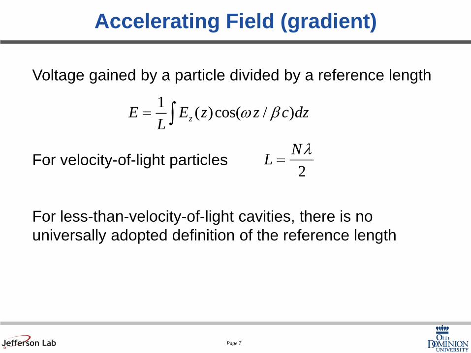
Accelerating Field (gradient)
Voltage gained by a particle divided by a reference length
For velocity-of-light particles
For less-than-velocity-of-light cavities, there is no
universally adopted definition of the reference length
1( )cos( / )zE E z z c dz
Lw b= ò
2
NL
l=

Page 8
Design Considerations
,max
,max
2
2
2
2
2
minimum critical field
minimum field emission
minimum shunt impedance, current losses
minimum dielectric losses
minimum control of microphonics
maximum
s
acc
s
acc
s
acc
s
acc
acc
H
E
E
E
H
E
E
E
U
E
< >
< >
voltage drop for high charge per bunch

Page 9
Energy Content
Energy density in electromagnetic field:
Because of the sinusoidal time dependence and the 90º
phase shift, he energy oscillates back and forth between
the electric and magnetic field
Total energy content in the cavity:
( )2 2
0 0
1
2u e m= +E H
2 20 0
2 2V VU dV dV
e m= =ò òE H
Page 10
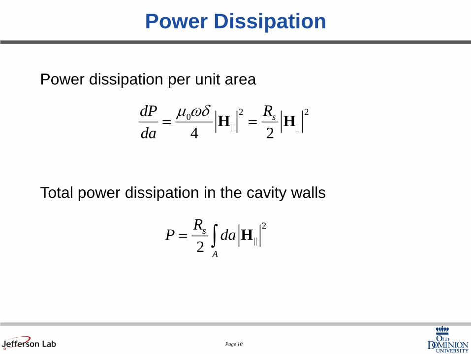
Power Dissipation
Power dissipation per unit area
Total power dissipation in the cavity walls
2 20
4 2
sRdP
da
m wd= =H H
2
2
s
A
RP da= ò H

Page 11
Quality Factor
Quality Factor Q0:
00
00 0
0
Energy stored in cavity
Energy dissipated in cavity walls per radian diss
UQ
P
w
ww t
w
º =
= =D
2
00 2
V
s
A
dVQ
R da
wm=
ò
ò
H
H

Page 12
Geometrical Factor
Geometrical Factor QRs (Ω)
Product of the Quality Factor and the surface resistance
Independent of size and material
Depends only on shape of cavity and electromagnetic mode
2 2 2
00 2 2 2
0
1 22
377 Impedance of vacuum
V V Vs
A A A
dV dV dVG QR
da da da
m phwm p
e l l
h
= = = =
» W
ò ò ò
ò ò ò
H H H
H H H

Page 13
Shunt Impedance, R/Q
Shunt impedance Rsh:
Vc = accelerating voltage
Note: Sometimes the shunt impedance is defined as
or quoted as impedance per unit length (ohm/m)
R/Q (in Ω)
2
in csh
diss
VR
Pº W
2
2c
diss
V
P
2 2 2R V P E L
Q P U Uw w= =

Page 14
Q – Geometrical Factor (Q Rs)
32 20 0
0
0 0
2 2 2
0
0
0
2 2 1 1
2 2 2 2 6
1 1 1
2 2 2
2006
Energy contentQ:
Energy disspated during one radian
Rough estimate (factor of 2) for fundamental mode
is si
s s
s
s
U
P
c LU H dv H
L
P R H dA R H L
QR
G QR
ww wt
w
m mp p pw
l e m
p
mp
e
= = =D
= =
= =
~ = W
=
ò
ò
275
ze (frequency) and material independent.
It depends only on the mode geometry
It is independent of number of cells
For superconducting elliptical cavities sQR W

Page 15
Shunt Impedance (Rsh), Rsh Rs, R/Q
( )
2 22
2 2
0
2
1 1
2 2
33,000
/ 100
/
In practice for elliptical cavities
per cell
per cell
and
Independent of size (frequency) and material
Depends on mode geometr
zsh
s
sh s
sh
sh s sh
E LVR
PR H L
R R
R Q
R R R Q
p
=
W
W
y
Proportional to number of cells

Page 16
Power Dissipated per Unit Length or Unit Area
2
12
1
2
1
2
2
2
1
For normal conductors
For superconductors
S
S
S
S
E RP
RLQR
Q
R
P
L
P
A
R
P
L
P
A
w
w
w
w
w
w
w
-
µ
µ
µ
µ
µ
µ
µ
Page 17
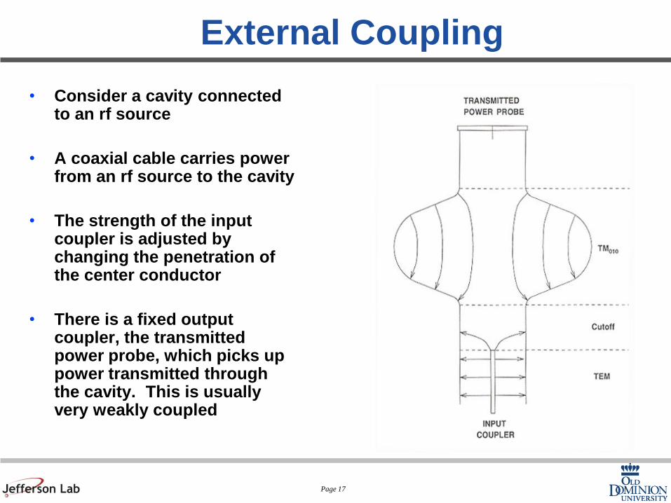
External Coupling
• Consider a cavity connected to an rf source
• A coaxial cable carries power from an rf source to the cavity
• The strength of the input coupler is adjusted by changing the penetration of the center conductor
• There is a fixed output coupler, the transmitted power probe, which picks up power transmitted through the cavity. This is usually very weakly coupled
Page 18
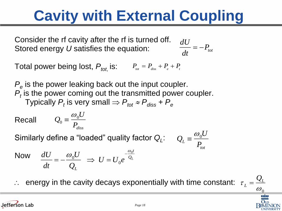
Cavity with External Coupling
Consider the rf cavity after the rf is turned off. Stored energy U satisfies the equation: Total power being lost, Ptot, is: Pe is the power leaking back out the input coupler. Pt is the power coming out the transmitted power coupler. Typically Pt is very small Ptot Pdiss + Pe Recall Similarly define a “loaded” quality factor QL: Now energy in the cavity decays exponentially with time constant:
tot diss e tP P P P= + +
0L
tot
UQ
P
wº
tot
dUP
dt= -
00
diss
UQ
P
wº
0
00
L
t
Q
L
UdUU U e
dt Q
ww -
= - Þ =
0
LL
Qt
w=

Page 19
Cavity with External Coupling
Equation
suggests that we can assign a quality factor to each loss mechanism, such that
where, by definition,
Typical values for CEBAF 7-cell cavities: Q0=1x10¹⁰, Qe QL=2x10⁷.
0 0
tot diss eP P P
U Uw w
+=
0
1 1 1
L eQ Q Q= +
0
e
e
UQ
P
wº

Page 20
Cavity with External Coupling
• Define “coupling parameter”:
therefore
is equal to:
• It tells us how strongly the couplers interact with the cavity.
Large implies that the power leaking out of the coupler is
large compared to the power dissipated in the cavity walls.
0
e
Q
Qb º
0
1 (1 )
LQ Q
b+=
e
diss
P
Pb =

Page 21
Several Loss Mechanisms
(
1 1
L
i
-wall losses
-power absorbed by beam
-coupling to outside world
Associate Q will each loss mechanism
index 0 is reserved for wall losses)
Loaded Q: Q
Coupling co
i
i
i
i
L
P P
UQ
P
P
Q U Q
w
w
=
=
= =
å
åå
0
0
0
1
efficient: ii
i
L
i
Q P
Q P
b
b
= =
=+å

Page 22
Equivalent Circuit for an rf Cavity
Simple LC circuit representing
an accelerating resonator
Metamorphosis of the LC circuit
into an accelerating cavity
Chain of weakly coupled pillbox
cavities representing an accelerating
cavity
Chain of coupled pendula as
its mechanical analogue

Page 23
Parallel Circuit Model of an Electromagnetic Mode
• Power dissipated in resistor R:
• Shunt impedance:
• Quality factor of resonator:
21
2
cdiss
VP
R=
2
csh
diss
VR
Pº 2shR RÞ =
1/2
0
0 0
diss c
U R CQ CR R
P L L
ww
w
æ öº = = = ç ÷è ø
1
0
0
0
1Z R iQww
w w
-
é ùæ ö= + -ê úç ÷è øë û
1
0
0 0
0
1 2Z R iQw w
w ww
-
é ùæ ö-» » +ê úç ÷è øë û
,

Page 24
1-Port System
2 2 00 0
00
0
1 21 2
g
g
kV RI V kV
R Qk Z R k Z iQi
www
w
= =æ ö
+ + + Dç ÷è ø+ D
2
00
0
1 2
Total impedance: R
k ZQ
i ww
+
+ D

Page 25
1-Port System
( )
( )
2 20
22 20
22
2 4 2 2
0 0 0
0
2
0
2
0 0
0
2 22
00
0
1 1
2 2
1
24
8
4 1
1 21
1
Energy content
Incident power:
Define coupling coefficient:
g
g
inc
inc
QU CV V
R
Q Rk V
RR k Z k Z Q
VP
Z
R
k Z
QU
P Q
w
w w
w
b
b
w b w
b w
= =
=æ öD
+ + ç ÷è ø
=
=
=+ æ öæ ö D
+ ç ÷ ç ÷+è ø è ø

Page 26
1-Port System
( )
( )
2 22
00
0
2
4 1
1 21
1
0, 1 :
4 11
1 21
Power dissipated
Optimal coupling: maximum or
critical coupling
Reflected power
diss inc
diss inc
inc
ref inc diss mc
UP P
Q Q
UP P
P
P P P P
w b
b w
b w
w b
b
b
= =+ æ öæ ö D
+ ç ÷ ç ÷+è ø è ø
=
Þ D = =
= - = -+
+
2
0
01
Q w
b w
é ùê úê úê ú
æ öDê úç ÷ê ú+è øë û
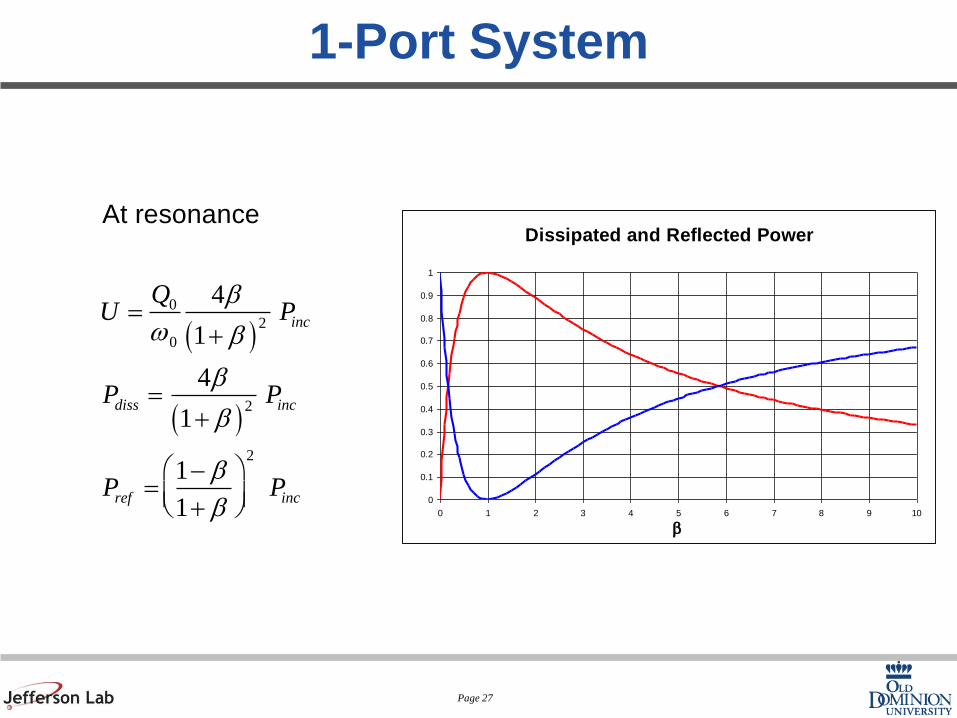
Page 27
1-Port System
( )
( )
0
2
0
2
2
4
1
4
1
1
1
At resonance
inc
diss inc
ref inc
QU P
P P
P P
b
w b
b
b
b
b
=+
=+
æ ö-= ç ÷+è ø
Dissipated and Reflected Power
0
0.1
0.2
0.3
0.4
0.5
0.6
0.7
0.8
0.9
1
0 1 2 3 4 5 6 7 8 9 10
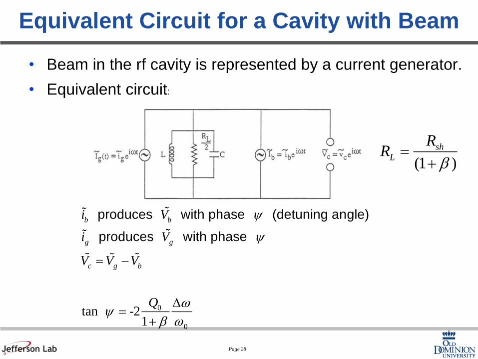
Page 28
Equivalent Circuit for a Cavity with Beam
• Beam in the rf cavity is represented by a current generator.
• Equivalent circuit:
(1 )
shL
RR
b=
+
0
0
tan -21
produces with phase (detuning angle)
produces with phase
b b
g g
c g b
i V
i V
V V V
Q
y
y
wy
b w
= -
D=
+
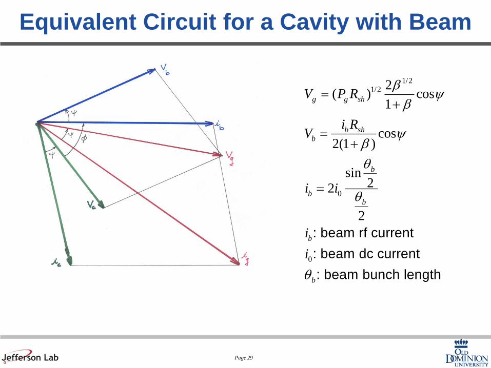
Page 29
Equivalent Circuit for a Cavity with Beam
1/21/2
0
0
2( ) cos
1
cos2(1 )
sin22
2
: beam rf current
: beam dc current
: beam bunch length
g g sh
b shb
b
bb
b
b
V P R
i RV
i i
i
i
by
b
yb
q
q
q
=+
=+
=
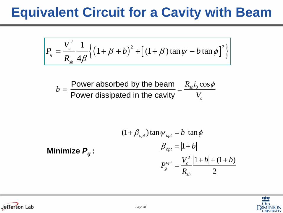
Page 30
Equivalent Circuit for a Cavity with Beam
( ) [ ]{ }2
2211 (1 ) tan tan
4
c
g
sh
VP b b
Rb b y f
b= + + + + -
0 cosPower absorbed by the beam =
Power dissipated in the cavitysh
c
R ib
V
f=
2
(1 ) tan tan
1
1 (1 )
2
opt opt
opt
opt cg
sh
b
b
b bVP
R
b y f
b
+ =
= +
+ + +=
Minimize Pg :

Page 31
Cavity with Beam and Microphonics
• The detuning is now
0 0
0 0
0
0tan 2 tan 2
where is the static detuning (controllable)
and is the random dynamic detuning (uncontrollable)
m
L L
m
Q Qdw dw dw
y yw w
dw
dw
±= - = -
-10
-8
-6
-4
-2
0
2
4
6
8
10
90 95 100 105 110 115 120
Time (sec)
Fre
qu
en
cy
(H
z)
Probability Density
Medium CM Prototype, Cavity #2, CW @ 6MV/m
400000 samples
0
0.05
0.1
0.15
0.2
0.25
-8 -6 -4 -2 0 2 4 6 8
Peak Frequency Deviation (V)
Pro
ba
bilit
y D
en
sit
y

Page 32
Qext Optimization with Microphonics
2
2
0
0
22
2
0
0
( 1) 2
( 1) ( 1) 22
mopt
opt c mg
sh
b Q
VP b b Q
R
dwb
w
dw
w
æ ö= + + ç ÷è ø
é ùæ ö
ê ú= + + + + ç ÷ê úè øë û
Condition for optimum coupling:
and
In the absence of beam (b=0):
and
2
0
0
22
0
0
1 2
1 1 22
If is very large
mopt
opt c mg
sh
m m
Q
VP Q
R
U
dwb
w
dw
w
dw dw
æ ö= + ç ÷è ø
é ùæ ö
ê ú= + + ç ÷ê úè øë û
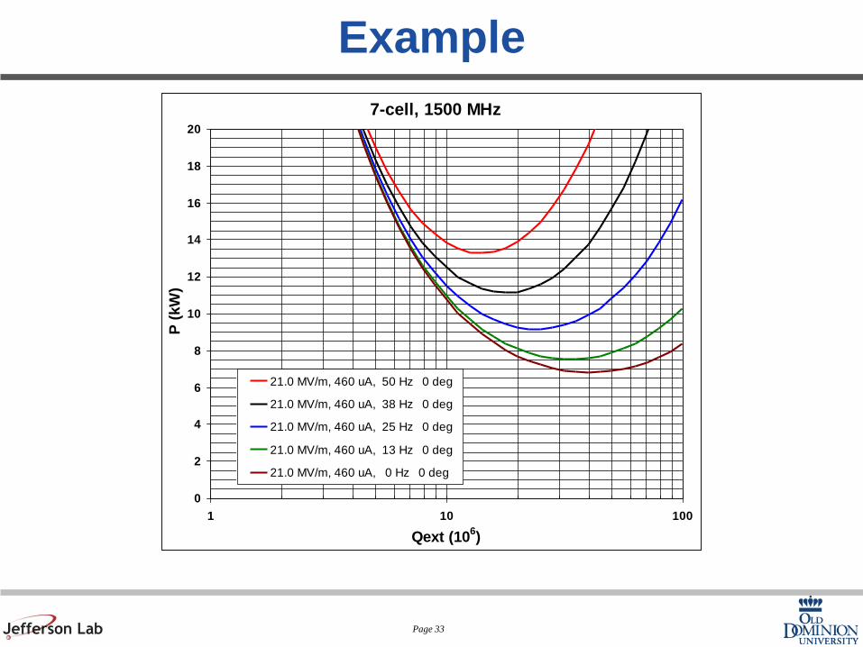
Page 33
Example
7-cell, 1500 MHz
0
2
4
6
8
10
12
14
16
18
20
1 10 100
Qext (106)
P (
kW
)
21.0 MV/m, 460 uA, 50 Hz 0 deg
21.0 MV/m, 460 uA, 38 Hz 0 deg
21.0 MV/m, 460 uA, 25 Hz 0 deg
21.0 MV/m, 460 uA, 13 Hz 0 deg
21.0 MV/m, 460 uA, 0 Hz 0 deg

Page 34
Another Simple Model:
Coaxial Half-wave Resonator
2b
2a
L

Page 35
Coaxial Half-wave Resonator
Capacitance per unit length
Inductance per unit length
0 0
0
2 2
1ln ln
Cb
a
pe pe
r
= =æ ö æ öç ÷ ç ÷è ø è ø
0 0
0 0
1ln ln
2 2
bL
r
m m
p p r
æ ö æ ö= =ç ÷ ç ÷è ø è ø
2b
2a
L
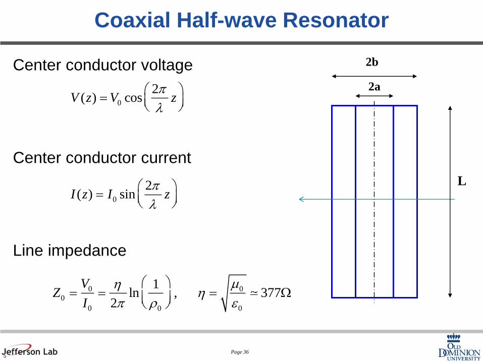
Page 36
Center conductor voltage
Center conductor current
Line impedance
Coaxial Half-wave Resonator
0
2( ) cosV z V z
p
l
æ ö= ç ÷è ø
0
2( ) sinI z I z
p
l
æ ö= ç ÷è ø
0 0
0
0 0 0
1ln , 377
2
VZ
I
mhh
p r e
æ ö= = = Wç ÷è ø
2b
2a
L

Page 37
Coaxial Half-wave Resonator
d: coaxial cylinders
Vp : Voltage on center conductor
Outer conductor at ground
Ep: Peak field on center conductor
Peak Electric Field

Page 38
Peak magnetic field
Coaxial Half-wave Resonator
0
0
1ln
300
9
m, A/m
m, T
cm, G
: Voltage across loading capacitance
mT at 1 MV/m
p
p
HV
c Bb
B
V
B
h
rr
ì ü ì üæ öï ï ï ï
= í ý í ýç ÷è øï ï ï ïî þ î þ
2b
2a
L
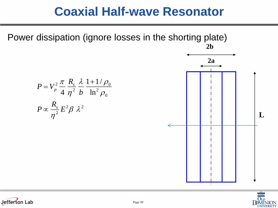
Page 39
Power dissipation (ignore losses in the shorting plate)
Coaxial Half-wave Resonator
2 0
2 2
0
2 2
2
1 1/
4 ln
sp
s
RP V
b
RP E
rp l
h r
b lh
+=
µ
2b
2a
L

Page 40
Energy content
Coaxial Half-wave Resonator
( )2 0
0
2 2 3
0
1
4 ln 1/pU V
U E
pel
r
e b l
=
µ
2b
2a
L

Page 41
Geometrical factor
Coaxial Half-wave Resonator
( )0
0
ln 1/2
1 1/s
bG QR
G
rp h
l r
h b
= =+
µ
2b
2a
L
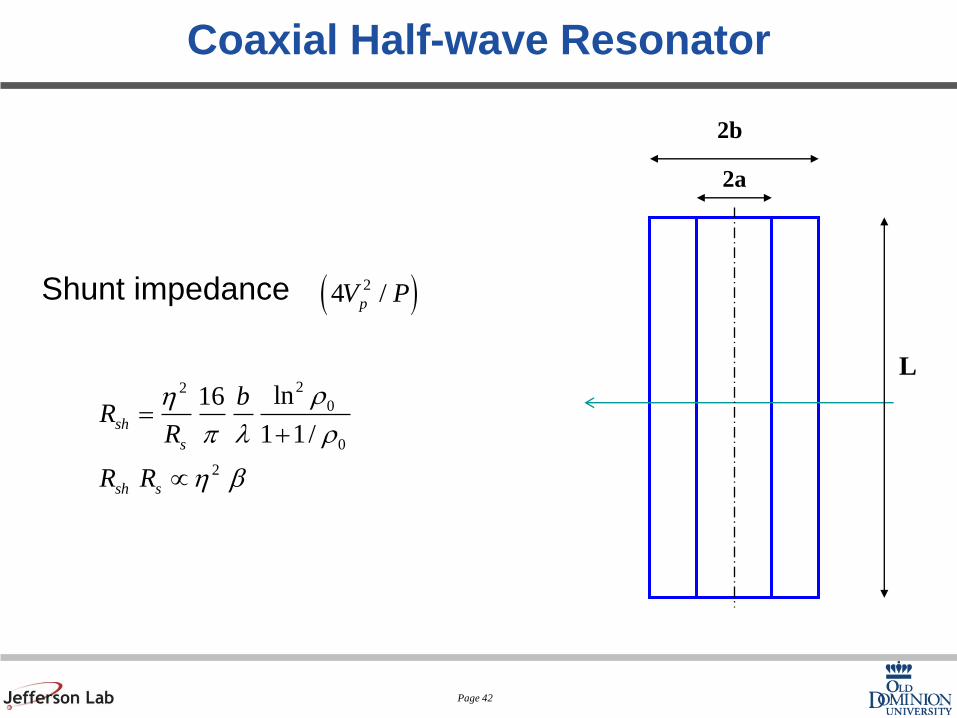
Page 42
Shunt impedance
Coaxial Half-wave Resonator
22
0
0
2
ln16
1 1/sh
s
sh s
bR
R
R R
rh
p l r
h b
=+
µ
( )24 /pV P
2b
2a
L
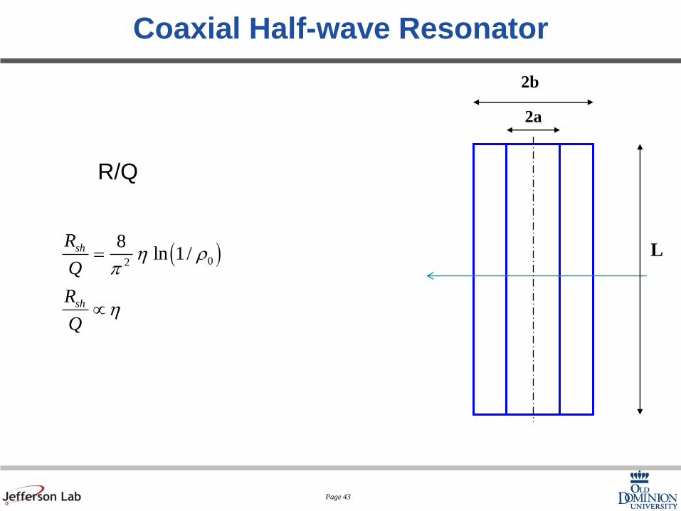
Page 43
R/Q
Coaxial Half-wave Resonator
( )02
8ln 1/sh
sh
R
Q
R
Q
h rp
h
=
µ
2b
2a
L

Page 44
Some Real Geometries (l/4)

Page 45
Some Real Geometries (l/4)
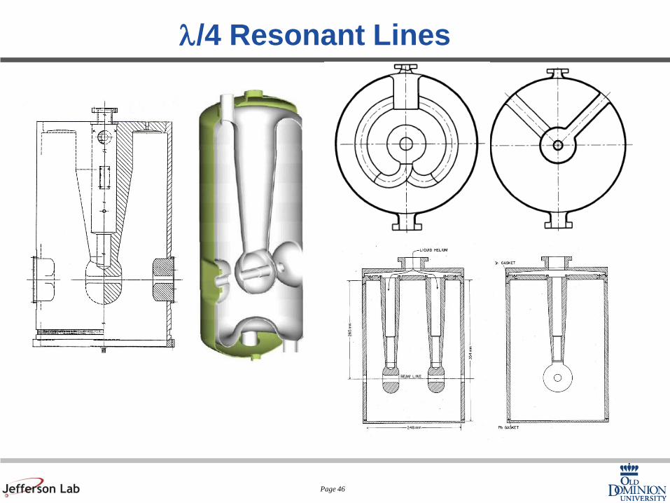
Page 46
l/4 Resonant Lines

Page 47
l/2 Resonant Lines
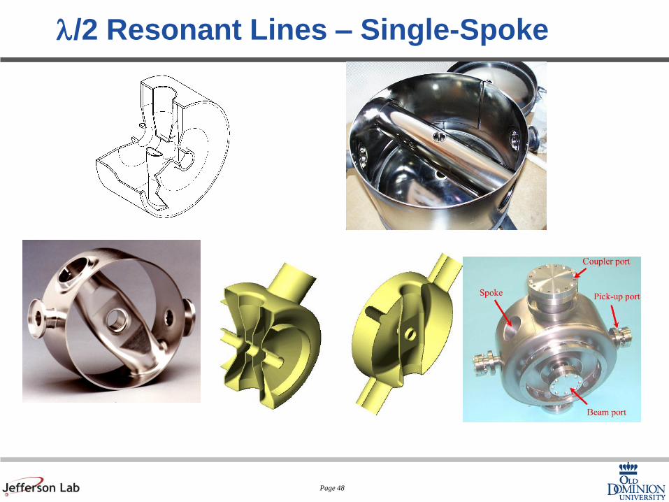
Page 48
l/2 Resonant Lines – Single-Spoke

Page 49
l/2 Resonant Lines – Double and Triple-Spoke

Page 50
l/2 Resonant Lines – Multi-Spoke

Page 51
1300 MHz 9-cell

Page 52
Pill Box Cavity
Hollow right cylindrical enclosure
Operated in the TM010 mode
0zH =
2 2
2 2 2
1 1z z zE E E
r r r c t
¶ ¶ ¶+ =
¶ ¶ ¶0
2.405c
Rw =
0
0 0( , , ) 2.405i t
z
rE r z t E J e
R
w-æ ö= ç ÷è ø
001
0
( , , ) 2.405i tE r
H r z t i J ec R
w
jm
-æ ö= - ç ÷è ø
E
TM010 mode

Page 53
Modes in Pill Box Cavity
• TM010
– Electric field is purely longitudinal
– Electric and magnetic fields have no angular
dependence
– Frequency depends only on radius, independent on
length
• TM0mn
– Monopoles modes that can couple to the beam and
exchange energy
• TM1mn
– Dipole modes that can deflect the beam
• TE modes
– No longitudinal E field
– Cannot couple to the beam
Page 54
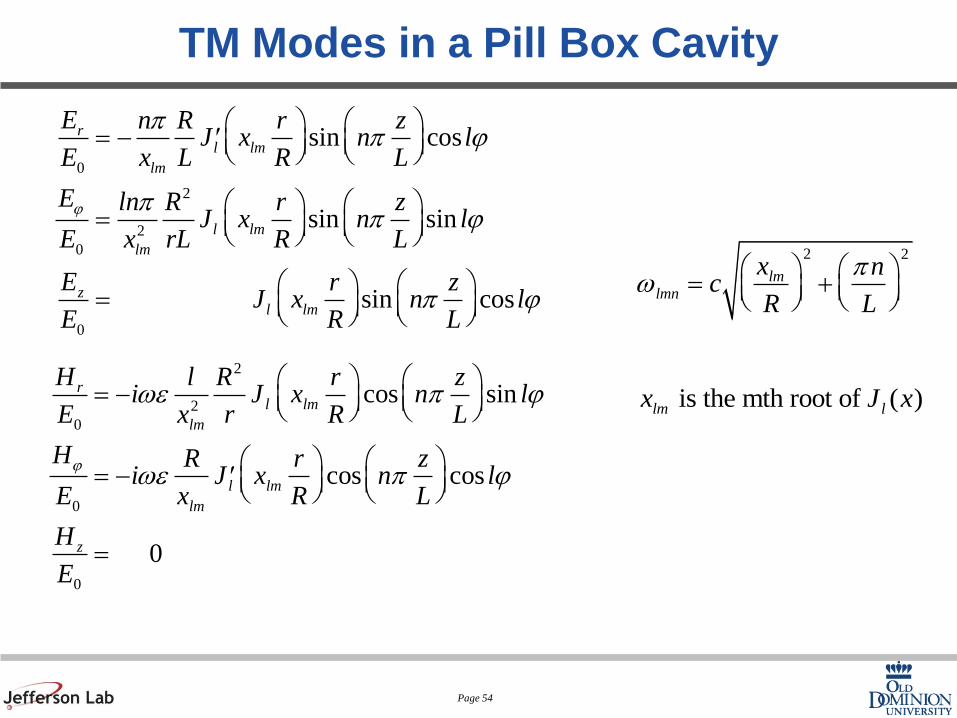
TM Modes in a Pill Box Cavity
0
2
2
0
0
sin cos
sin sin
sin cos
rl lm
lm
l lm
lm
zl lm
E n R r zJ x n l
E x L R L
E ln R r zJ x n l
E x rL R L
E r zJ x n l
E R L
j
pp j
pp j
p j
æ ö æ ö= - ¢ç ÷ ç ÷è ø è ø
æ ö æ ö= ç ÷ ç ÷è ø è ø
æ ö æ ö= ç ÷ ç ÷è ø è ø
2
2
0
0
0
cos sin
cos cos
0
rl lm
lm
l lm
lm
z
H l R r zi J x n l
E x r R L
H R r zi J x n l
E x R L
H
E
j
we p j
we p j
æ ö æ ö= - ç ÷ ç ÷è ø è ø
æ ö æ ö= - ¢ç ÷ ç ÷è ø è ø
=
is the mth root of ( )lm lx J x
2 2
lmlmn
x nc
R L
pw
æ ö æ ö= + ç ÷ç ÷ è øè ø

Page 55
TM010 Mode in a Pill Box Cavity
0 0 01
0 1 01
01
01 01
01
0
0
2.405
0.3832
r z
r z
rE E E E J x
R
R rH H H i E J x
x R
cx x
R
xR
j
j we
w
l lp
æ ö= = = ç ÷è ø
æ ö= = = - ç ÷è ø
= =
= =

Page 56
TM010 Mode in a Pill Box Cavity
Energy content
Power dissipation
Geometrical factor
2 2 2
0 0 1 01( )2
U E J x LRp
e=
2 2
0 1 012( )( )sR
P E J x R L Rph
= +
01
2 ( )
x LG
R Lh=
+
01
1 01
2.40483
( ) 0.51915
x
J x
=
=

Page 57
TM010 Mode in a Pill Box Cavity
Energy Gain
Gradient
Shunt impedance
0 sinL
W El p
p lD =
2 22
3 2
1 01
1sin
( ) ( )sh
s
LR
R J x R R L
h l p
p l
æ ö= ç ÷è ø+
0
2sin
/ 2acc
W LE E
p
l p l
D= =

Page 58
Real Cavities
Beam tubes reduce the electric field on axis
Gradient decreases
Peak fields increase
R/Q decreases

Page 59
Real Cavities
Page 60
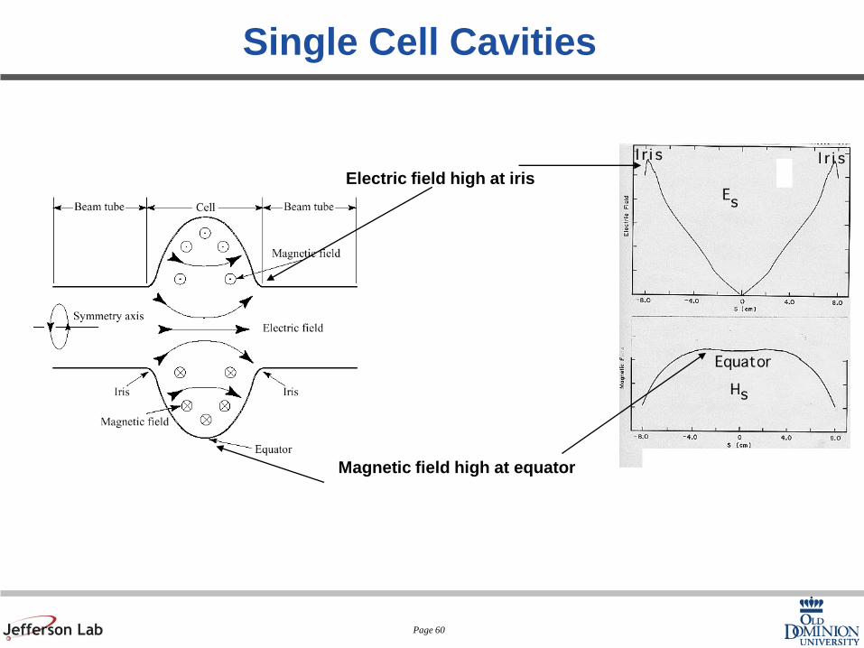
Single Cell Cavities
Electric field high at iris
Magnetic field high at equator

Page 61
Coupling between cells
+ +
+ -
Symmetry plane for
the H field
Symmetry plane for
the E field
which is an additional
solution
ωo
ωπ
0
0cck
2
p
p
w w
w w
-=
+
The normalized
difference between these
frequencies is a measure
of the energy flow via the
coupling region

Page 62
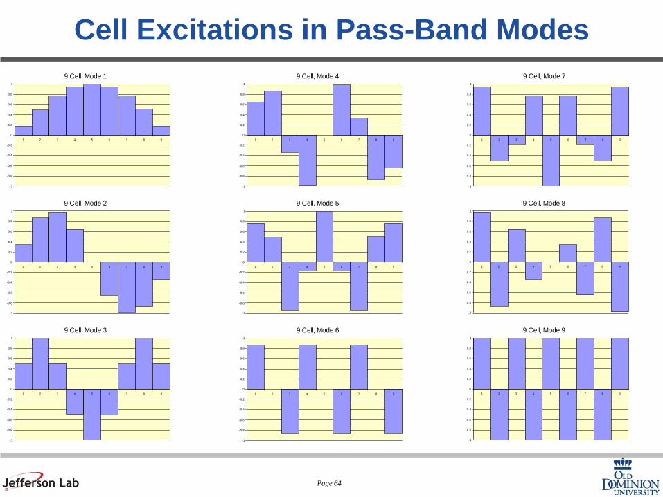
Multi-Cell Cavities
Mode frequencies:
Voltages in cells:
2
2
0
2
1
0
1 2 1 cos
1 cos2
m
n n
mk
n
kk
n n
w p
w
w w p p
w-
æ ö= + -ç ÷è ø
- æ ö æ ö-ç ÷ ç ÷è ø è ø
2 1sin
2
m
j
jV m
np
-æ ö= ç ÷è ø
/ 2b k
k
Ck C C
C= =

Page 63
Pass-Band Modes Frequencies
-1
0 1 2 3 4 5 6 7 8 9
9-cell cavity
0w
1/2
0 (1 4 )kw +
Page 64
Cell Excitations in Pass-Band Modes
9 Cell, Mode 1
-1
-0.8
-0.6
-0.4
-0.2
0
0.2
0.4
0.6
0.8
1
1 2 3 4 5 6 7 8 9
9 Cell, Mode 2
-1
-0.8
-0.6
-0.4
-0.2
0
0.2
0.4
0.6
0.8
1
1 2 3 4 5 6 7 8 9
9 Cell, Mode 3
-1
-0.8
-0.6
-0.4
-0.2
0
0.2
0.4
0.6
0.8
1
1 2 3 4 5 6 7 8 9
9 Cell, Mode 4
-1
-0.8
-0.6
-0.4
-0.2
0
0.2
0.4
0.6
0.8
1
1 2 3 4 5 6 7 8 9
9 Cell, Mode 5
-1
-0.8
-0.6
-0.4
-0.2
0
0.2
0.4
0.6
0.8
1
1 2 3 4 5 6 7 8 9
9 Cell, Mode 6
-1
-0.8
-0.6
-0.4
-0.2
0
0.2
0.4
0.6
0.8
1
1 2 3 4 5 6 7 8 9
9 Cell, Mode 7
-1
-0.8
-0.6
-0.4
-0.2
0
0.2
0.4
0.6
0.8
1
1 2 3 4 5 6 7 8 9
9 Cell, Mode 8
-1
-0.8
-0.6
-0.4
-0.2
0
0.2
0.4
0.6
0.8
1
1 2 3 4 5 6 7 8 9
9 Cell, Mode 9
-1
-0.8
-0.6
-0.4
-0.2
0
0.2
0.4
0.6
0.8
1
1 2 3 4 5 6 7 8 9
Page 65
Jean Delayen
Center for Accelerator Science
Old Dominion University
and
Thomas Jefferson National Accelerator Facility
SRF FUNDAMENTALS
ODU TAAD I Fall 2012

Page 66
Historical Overview
Page 67
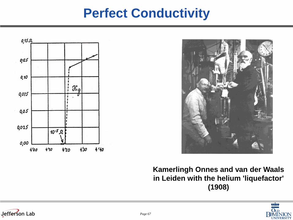
Perfect Conductivity
Kamerlingh Onnes and van der Waals
in Leiden with the helium 'liquefactor'
(1908)
Page 68
Perfect Conductivity
Persistent current experiments on rings have measured
1510s
n
s
s>
Perfect conductivity is not superconductivity
Superconductivity is a phase transition
A perfect conductor has an infinite relaxation time L/R
Resistivity < 10-23 Ω.cm
Decay time > 105 years

Page 69
Perfect Diamagnetism (Meissner & Ochsenfeld 1933)
0B
t
¶=
¶0B =
Perfect conductor Superconductor

Page 70
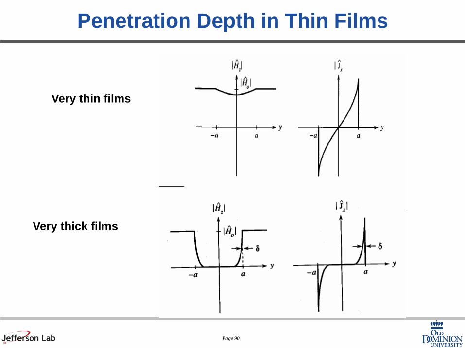
Penetration Depth in Thin Films
Very thin films
Very thick films

Page 71
Critical Field (Type I)
2
( ) (0) 1c c
c
TH T H
T
é ùæ öê ú- ç ÷è øê úë û
Superconductivity is destroyed by the application of a magnetic field
Type I or “soft” superconductors

Page 72
Critical Field (Type II or “hard” superconductors)
Expulsion of the magnetic field is complete up to Hc1, and partial up to Hc2
Between Hc1 and Hc2 the field penetrates in the form if quantized vortices
or fluxoids
0e
pf =

Page 73
Thermodynamic Properties
Entropy Specific Heat
Energy Free Energy
Page 74
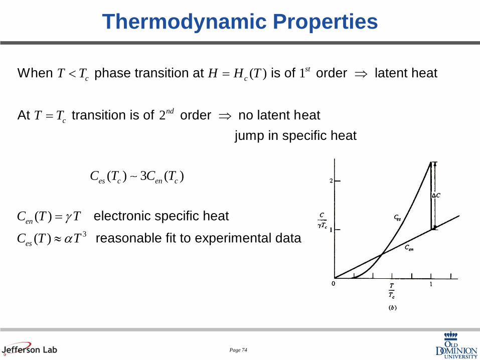
Thermodynamic Properties
( ) 1
2
When phase transition at is of order latent heat
At transition is of order no latent heat
jump in specific heat
st
c c
nd
c
es
T T H H T
T T
C
< = Þ
= Þ
3
( ) 3 ( )
( )
( )
electronic specific heat
reasonable fit to experimental data
c en c
en
es
T C T
C T T
C T T
g
a
=
»
Page 75
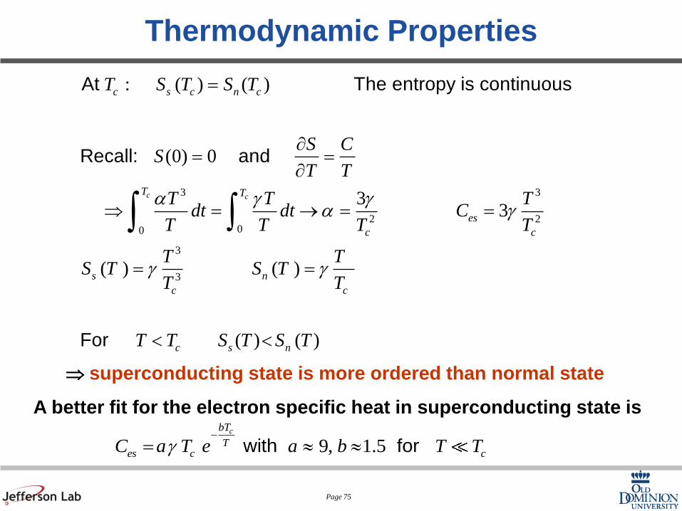
Thermodynamic Properties
3 3
2 200
3
3
: ( ) ( )
(0) 0
33
( ) ( )
( ) ( )
At The entropy is continuous
Recall: and
For
c c
c s c n c
T T
es
c c
s n
c c
c s n
T S T S T
S CS
T T
T T Tdt dt C
T T T T
T TS T S T
T T
T T S T S T
a g ga g
g g
=
¶= =
Þ = ® = =
= =
< <
òò
superconducting state is more ordered than normal state
A better fit for the electron specific heat in superconducting state is
9, 1.5 with for cbT
Tes c cC a T e a b T Tg
-
= » »
Page 76
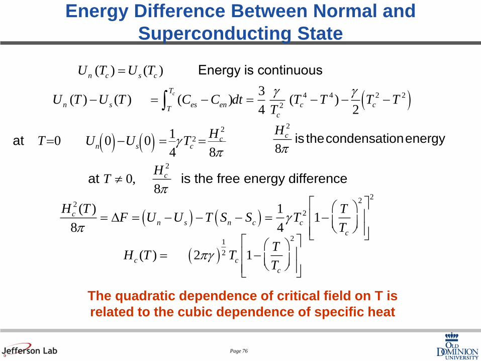
( )4 4 2 2
2
( ) ( )
3( ) ( ) ( ) ( )
4 2
Εnergy is continuous
c
n c s c
T
n s es en c cT
c
U T U T
U T U T C C dt T T T TT
g g
=
- = - = - - -ò
( ) ( )2
210 0 0
4 8at c
n s c
HT U U Tg
p= - = =
2
8is thecondensationenergycH
p
2
0,8
at is the free energy differencecHT
p¹
( ) ( )
22
22( ) 1
18 4
cn s n c c
c
H T TF U U T S S T
Tg
p
é ùæ öê ú= D = - - - = - ç ÷è øê úë û
( )21
2( ) 2 1c c
c
TH T T
Tpg
é ùæ öê ú= - ç ÷è øê úë û
The quadratic dependence of critical field on T is
related to the cubic dependence of specific heat
Energy Difference Between Normal and
Superconducting State

Page 77
Isotope Effect (Maxwell 1950)
The critical temperature and the critical field at 0K are dependent
on the mass of the isotope
(0) with 0.5c cT H M a a-

Page 78
Energy Gap (1950s)
At very low temperature the specific heat exhibits an exponential behavior
Electromagnetic absorption shows a threshold
Tunneling between 2 superconductors separated by a thin oxide film
shows the presence of a gap
/1.5 with cbT T
sc e b-
µ

Page 79
Two Fundamental Lengths
• London penetration depth λ
– Distance over which magnetic fields decay in
superconductors
• Pippard coherence length ξ
– Distance over which the superconducting state decays

Page 80
Two Types of Superconductors
• London superconductors (Type II)
– λ>> ξ
– Impure metals
– Alloys
– Local electrodynamics
• Pippard superconductors (Type I)
– ξ >> λ
– Pure metals
– Nonlocal electrodynamics

Page 81
Material Parameters for Some Superconductors
Page 82
Phenomenological Models (1930s to 1950s)
Phenomenological model:
Purely descriptive
Everything behaves as though…..
A finite fraction of the electrons form some kind of condensate
that behaves as a macroscopic system (similar to superfluidity)
At 0K, condensation is complete
At Tc the condensate disappears

Page 83
Two Fluid Model – Gorter and Casimir
( )
( )
( )
1/2
2
2
(1 ) :
( ) = ( ) (1 ) ( )
1
2
1
4
gives
c
n s
n
s c
T T x
x
F T x f T x f T
f T T
f T T
F T
g
b g
< =
-
+ -
= -
= - =-
fractionof "normal"electrons
fractionof "condensed"electrons (zero entropy)
Assume: free energy
independent of temperature
Minimizationof
C
4
4
1/2
3
2
=
( ) ( ) (1 ) ( ) 1
T3
T
C
n s
C
es
Tx
T
TF T x f T x f T
T
C
b
g
æ öç ÷è ø
é ùæ öê úÞ = + - = - + ç ÷è øê úë û
Þ =

Page 84
Two Fluid Model – Gorter and Casimir
4
1/2
2
2
2
( ) ( ) (1 ) ( ) 1
( ) ( ) 22
8
1
n s
C
n
C
c
TF T x f T x f T
T
TF T f T T
T
H
T
T
b
gb
p
b
é ùæ öê ú= + - = - + ç ÷è øê úë û
æ ö= = - = - ç ÷è ø
=
= -
Superconducting state:
Normal state:
Recall difference in free energy between normal and
superconducting state
22 2
( )1
(0)
c
C c C
H T T
H T
é ùæ ö æ öê ú Þ = -ç ÷ ç ÷è ø è øê úë û
The Gorter-Casimir model is an “ad hoc” model (there is no physical basis
for the assumed expression for the free energy) but provides a fairly
accurate representation of experimental results

Page 85
Model of F & H London (1935)
Proposed a 2-fluid model with a normal fluid and superfluid components
ns : density of the superfluid component of velocity vs
nn : density of the normal component of velocity vn
2
superelectrons are accelerated by
superelectrons
normal electrons
s s
s s
n n
m eE Et
J en
J n eE
t m
J E
u
u
s
¶= -
= -
¶=
=

Page 86
Model of F & H London (1935)
2
2 2
2
0 = Constant
= 0
Maxwell:
F&H London postulated:
s s
s s
s s
s
s
J n eE
t m
BE
t
m mJ B J B
t n e n e
mJ B
n e
¶=
¶Ñ´ = -
æ ö¶Þ Ñ´ + = Þ Ñ´ +ç ÷¶ è ø
Ñ´ +
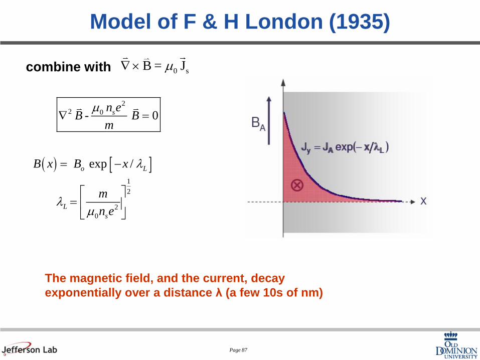
Page 87
Model of F & H London (1935)
combine with 0 sB = JmÑ´
( ) [ ]
22 0
1
2
2
0
- 0
exp /
s
o L
L
s
n eB B
m
B x B x
m
n e
m
l
lm
Ñ =
= -
é ù= ê úë û
The magnetic field, and the current, decay
exponentially over a distance λ (a few 10s of nm)

Page 88
1
2
2
0
4
14 2
1
1( ) (0)
1
L
s
s
C
L L
C
m
n e
Tn
T
T
T
T
lm
l l
é ù= ê úë û
é ùæ öê úµ - ç ÷è øê úë û
=
é ùæ ö-ê úç ÷è øê úë û
From Gorter and Casimir two-fluid model
Model of F & H London (1935)
Page 89
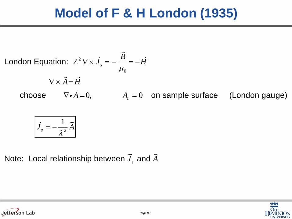
Model of F & H London (1935)
2
0
2
0, 0
1
London Equation:
choose on sample surface (London gauge)
Note: Local relationship between and
s
n
s
s
BJ H
A H
A A
J A
J A
lm
l
Ñ´ = - = -
Ñ´ =
Ñ = =
= -
Page 90
Penetration Depth in Thin Films
Very thin films
Very thick films

Page 91
Quantum Mechanical Basis for London Equation
2* * *
1
0
2
( ) ( ) ( )2
0 ( ) 0 ,
( )( ) ( )
( )
n n n n n
n
e eJ r A r r r dr dr
mi mc
A J r
r eJ r A r
m e
r n
y y y y y y d
y y
y
r
r
ì üé ù= Ñ - Ñ - - -í ýë û
î þ
= = =
= -
=
åò
In zero field
Assume is "rigid", ie the field has no effect on wave function
Page 92
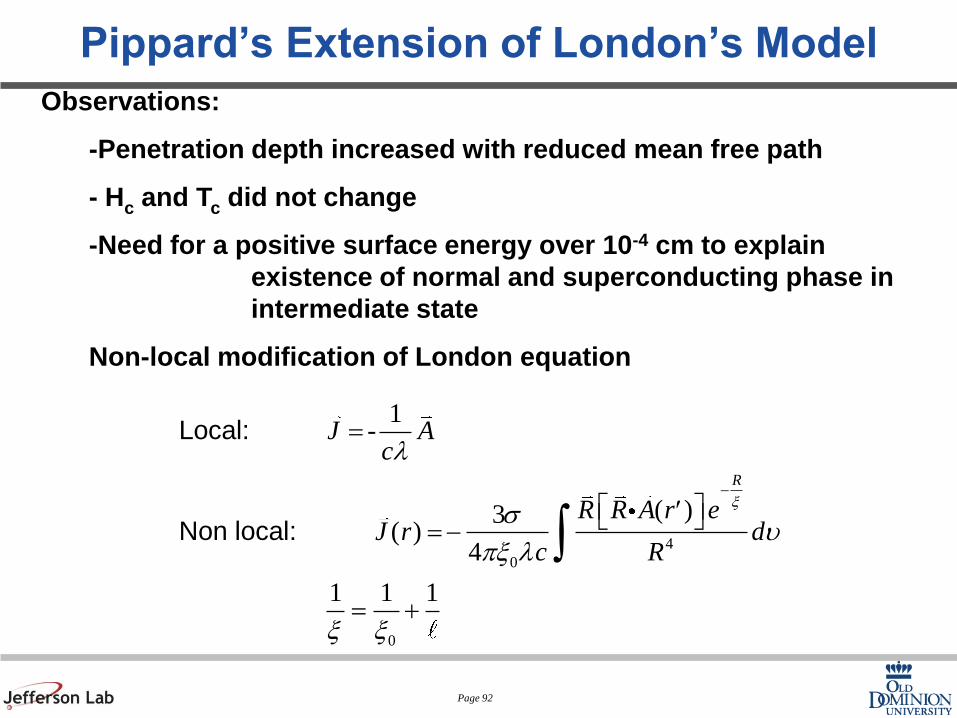
Pippard’s Extension of London’s Model
Observations:
-Penetration depth increased with reduced mean free path
- Hc and Tc did not change
-Need for a positive surface energy over 10-4 cm to explain
existence of normal and superconducting phase in
intermediate state
Non-local modification of London equation
4
0
0
1-
( )3( )
4
1 1 1
R
J Ac
R R A r eJ r d
c R
x
l
su
px l
x x
-
=
é ù¢ë û=-
= +
ò
Local:
Non local:

Page 93
London and Pippard Kernels
Apply Fourier transform to relationship between
( ) ( ) : ( ) ( ) ( )4
cJ r A r J k K k A k
p= - and
2
2
2
( )( )ln 1
eff effo
o
dk
K kK k kdk
k
pl l
p
¥
¥= =
+ é ù+ê úë û
òò
Specular: Diffuse:
Effective penetration depth

Page 94
London Electrodynamics
Linear London equations
together with Maxwell equations
describe the electrodynamics of superconductors at all T if:
– The superfluid density ns is spatially uniform
– The current density Js is small
2
2 2
0
10sJ E
H Ht l m l
¶= - Ñ - =
0s
HH J E
tm
¶Ñ´ = Ñ´ = -

Page 95
Ginzburg-Landau Theory
• Many important phenomena in superconductivity occur
because ns is not uniform
– Interfaces between normal and superconductors
– Trapped flux
– Intermediate state
• London model does not provide an explanation for the
surface energy (which can be positive or negative)
• GL is a generalization of the London model but it still
retain the local approximation of the electrodynamics
Page 96
Ginzburg-Landau Theory
• Ginzburg-Landau theory is a particular case of Landau’s theory of second order phase transition
• Formulated in 1950, before BCS
• Masterpiece of physical intuition
• Grounded in thermodynamics
• Even after BCS it still is very fruitful in analyzing the behavior of superconductors and is still one of the most widely used theory of superconductivity
Page 97
Ginzburg-Landau Theory
• Theory of second order phase transition is based on an order parameter which is zero above the transition temperature and non-zero below
• For superconductors, GL use a complex order parameter Ψ(r) such that |Ψ(r)|2 represents the density of superelectrons
• The Ginzburg-Landau theory is valid close to Tc
Page 98
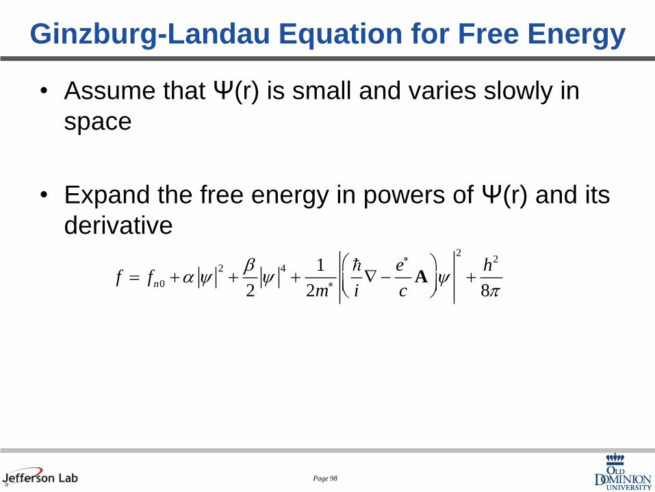
Ginzburg-Landau Equation for Free Energy
• Assume that Ψ(r) is small and varies slowly in
space
• Expand the free energy in powers of Ψ(r) and its
derivative 2
22 4
0
1
2 2 8n
e hf f
m i c
ba y y y
p
*
*
æ ö= + + + Ñ- +ç ÷è ø
A

Page 99
Field-Free Uniform Case
Near Tc we must have
At the minimum
2 4
02
nf fb
a y y- = +0
f fn
-0
f fn
-
yyy ¥
0a > 0a <
0 ( ) ( 1)t tb a a> = -¢
2 22
0 (1 )8 2
and cn c
Hf f H t
ay
p b- = - = - Þ µ -
2 ay
b¥ = -
Page 100
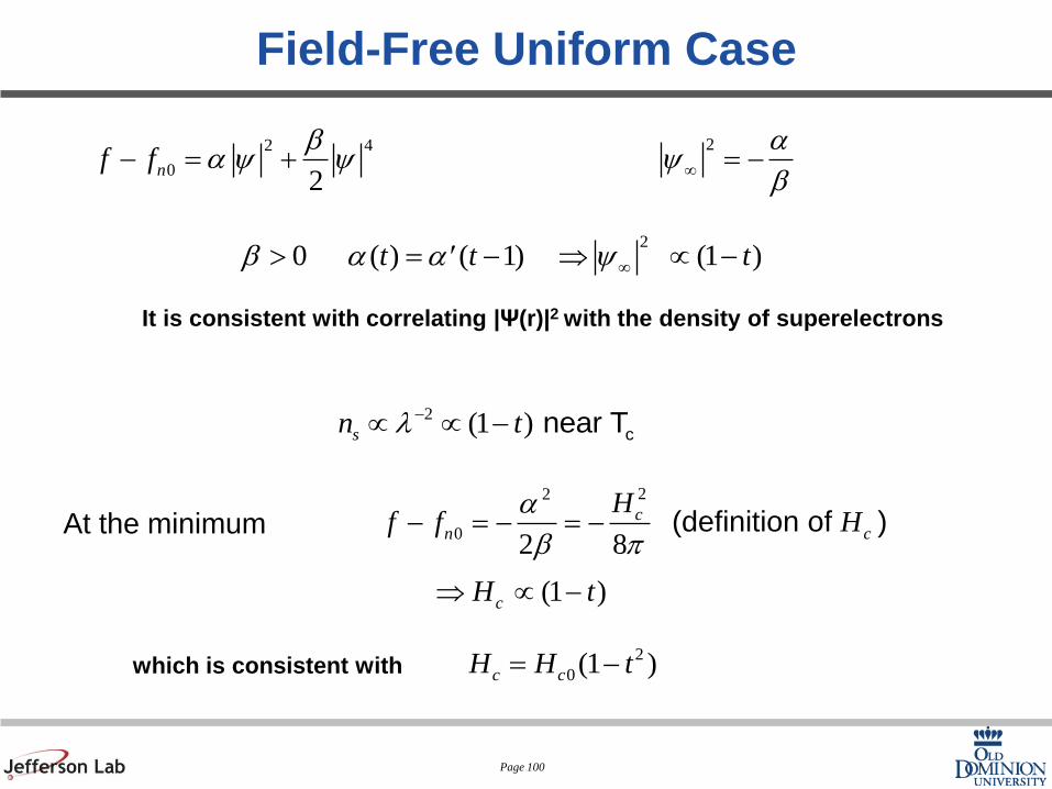
Field-Free Uniform Case
At the minimum
2 4
02
nf fb
a y y- = +
20 ( ) ( 1) (1 ) t t tb a a y ¥> = - Þ µ -¢
22
02 8
(1 )
(definition of )cn c
c
Hf f H
H t
a
b p- = - = -
Þ µ -
2 ay
b¥ = -
It is consistent with correlating |Ψ(r)|2 with the density of superelectrons
2 (1 ) c near Tsn tl -µ µ -
which is consistent with 2
0(1 )c cH H t= -
Page 101
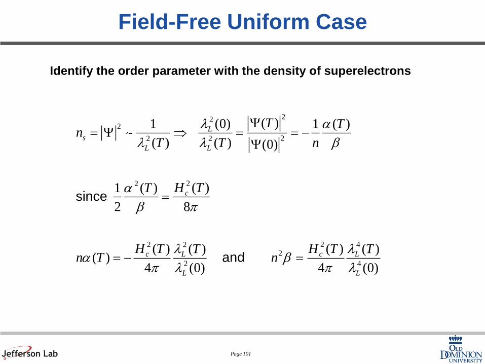
Field-Free Uniform Case
Identify the order parameter with the density of superelectrons
222
22 2
22
2 22 42
2 4
( )(0)1 1 ( )
( ) ( ) (0)
( )1 ( )
2 8
( ) ( )( ) ( )( )
4 (0) 4 (0)
since
and
Ls
L L
c
c cL L
L L
T Tn
T T n
H TT
H T H TT Tn T n
l a
l l b
a
b p
l la b
p l p l
Y= Y Þ = = -
Y
=
= - =

Page 102
Field-Free Nonuniform Case
Equation of motion in the absence of electromagnetic
field
221( ) 0
2T
my a y b y y
*- Ñ + + =
Look at solutions close to the constant one 2 ( )
whereTa
y y d yb
¥ ¥= + = -
To first order: 21
04 ( )m T
d da*
Ñ - =
Which leads to 2 / ( )r Te
xd
-»

Page 103
Field-Free Nonuniform Case
2 / ( )
2
(0)1 2( )
( ) ( )2 ( ) where
r T L
c L
ne T
m H T Tm T
x lpd x
la
-
**» = =
is the Ginzburg-Landau coherence length.
It is different from, but related to, the Pippard coherence length. ( )
0
1/22
( )1
Tt
xx
-
GL parameter: ( )
( )( )
L TT
T
lk
x=
( ) ( )
( )
Both and diverge as but their ratio remains finite
is almost constant over the whole temperature range
L cT T T T
T
l x
k
®

Page 104
2 Fundamental Lengths
London penetration depth: length over which magnetic field decay
Coherence length: scale of spatial variation of the order parameter
(superconducting electron density)
1/2
2( )
2
cL
c
TmT
e T T
bl
a
*æ ö= ç ÷ -¢è ø
1/22
( )4
c
c
TT
m T Tx
a*æ ö
= ç ÷ -¢è ø
The critical field is directly related to those 2 parameters
0( )2 2 ( ) ( )
c
L
H TT T
f
x l=

Page 105
Surface Energy
2 2
2
2
1
8
:8
:8
Energy that can be gained by letting the fields penetrate
Energy lost by "damaging" superconductor
c
c
H H
H
H
s x lp
l
p
x
p
é ù-ë û

Page 106
Surface Energy
2 2
c
Interface is stable if >0
If >0
Superconducting up to H where superconductivity is destroyed globally
If >> <0 for
Advantageous to create small areas of normal state with large
cH H
s
x l s
xl x s
l
>>
>
1:
2
1:
2
area to volume ratio
quantized fluxoids
More exact calculation (from Ginzburg-Landau):
= Type I
= Type II
lk
x
lk
x
®
<
>
2 21
8cH Hs x l
pé ù-ë û
Page 107
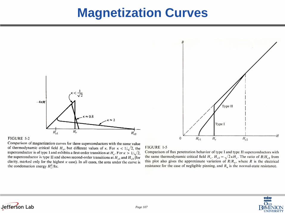
Magnetization Curves

Page 108
Intermediate State
Vortex lines in
Pb.98In.02 At the center of each vortex is a
normal region of flux h/2e

Page 109
Critical Fields
2
2
1
2
2
1(ln .008)
2
Type I Thermodynamic critical field
Superheating critical field
Field at which surface energy is 0
Type II Thermodynamic critical field
(for 1)
c
csh
c
c c
cc
c
c
H
HH
H
H H
HH
H
H
k
k
k kk
=
+
Even though it is more energetically favorable for a type I superconductor
to revert to the normal state at Hc, the surface energy is still positive up to
a superheating field Hsh>Hc → metastable superheating region in which
the material may remain superconducting for short times.
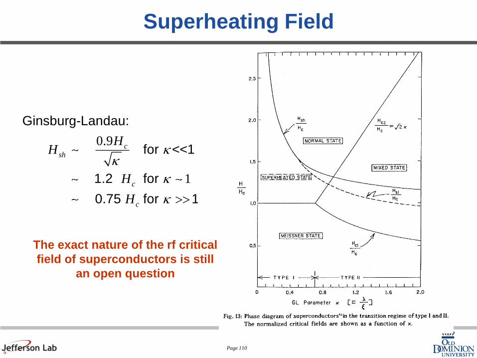
Page 110
Superheating Field
0.9
1
Ginsburg-Landau:
for <<1
1.2 for
0.75 for 1
csh
c
c
HH
H
H
kk
k
k >>
The exact nature of the rf critical
field of superconductors is still
an open question
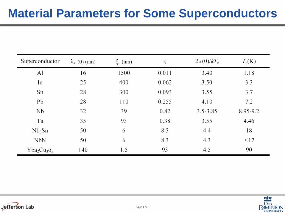
Page 111
Material Parameters for Some Superconductors

Page 112
BCS
• What needed to be explained and what were the
clues?
– Energy gap (exponential dependence of specific heat)
– Isotope effect (the lattice is involved)
– Meissner effect

Page 113
Cooper Pairs
Assumption: Phonon-mediated attraction between
electron of equal and opposite momenta located
within of Fermi surface
Moving electron distorts lattice and leaves behind a
trail of positive charge that attracts another electron
moving in opposite direction
Fermi ground state is unstable
Electron pairs can form bound
states of lower energy
Bose condensation of overlapping
Cooper pairs into a coherent
Superconducting state
Dw

Page 114
Cooper Pairs
One electron moving through the lattice attracts the positive ions.
Because of their inertia the maximum displacement will take place
behind.

Page 115
BCS
The size of the Cooper pairs is much larger than their spacing
They form a coherent state
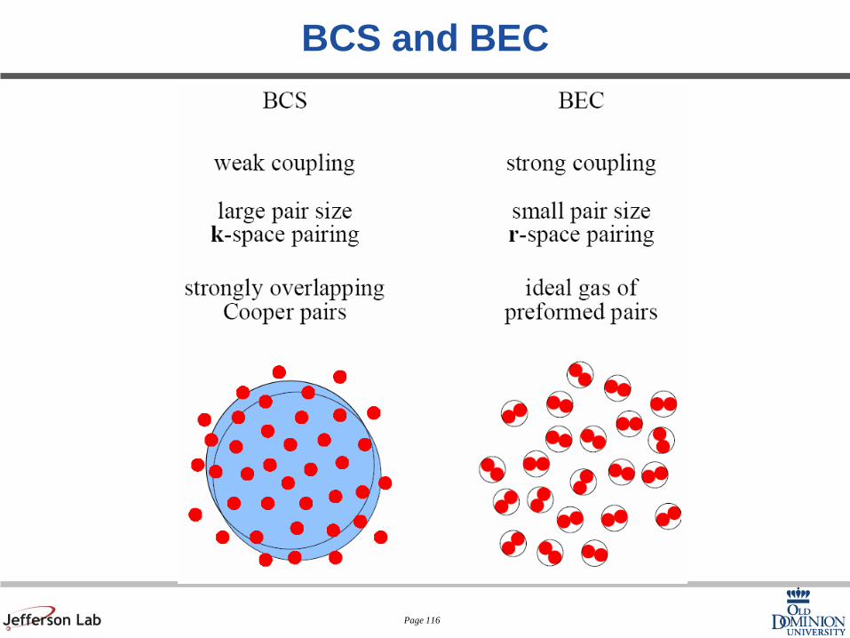
Page 116
BCS and BEC
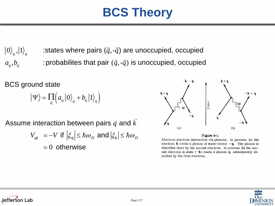
Page 117
BCS Theory
( )
0 , 1 ,-
, : ( ,- )
0 1
:states where pairs ( ) are unoccupied, occupied
probabilites that pair is unoccupied, occupied
BCS ground state
Assume interaction between pairs and
q q
q q
q qq qq
qk
q q
a b q q
a b
q k
V
Y = +
=
P
0
q k if and
otherwise
D DV x w x w- £ £
=

Page 118
BCS
• Hamiltonian
• Ground state wave function
destroys an electron of momentum
creates an electron of momentum
number of electrons of momentum
k k qk q q k k
k qk
k
q
k k k
n V c c c c
c k
c k
n c c k
e * *
- -
*
*
= +
=
å åH
( ) 0q q q qq
a b c c f* *
-Y = +P

Page 119
BCS
• The BCS model is an extremely simplified model of reality
– The Coulomb interaction between single electrons is ignored
– Only the term representing the scattering of pairs is retained
– The interaction term is assumed to be constant over a thin
layer at the Fermi surface and 0 everywhere else
– The Fermi surface is assumed to be spherical
• Nevertheless, the BCS results (which include only a very few
adjustable parameters) are amazingly close to the real world

Page 120
BCS
2
2 2
0
1
(0)
0
0, 1 0
1, 0 0
2 1
21
sinh(0)
q q q
q q q
q
q
q
VDD
a b
a b
b
e
V
r
x
x
x
x
ww
r
-
= = <
= = >
= -+ D
D =é ùê úë û
Is there a state of lower energy than
the normal state?
for
for
yes:
where

Page 121
BCS
( )
11.14 exp
( )
0 1.76
c D
F
c
kTVN E
kT
wé ù
= -ê úë û
D =
Critical temperature
Coherence length (the size of the Cooper pairs)
0 .18 F
ckT
ux =

Page 122
BCS Condensation Energy
2
0
2
0 00
0
4
(0)
2
8
/ 10
/ 10
s n
F
VE E
HN
k K
k K
r
e p
e
D- = -
æ öD- D =ç ÷è ø
D
F
Condensation energy:

Page 123
BCS Energy Gap
At finite temperature:
Implicit equation for the temperature dependence of the gap:
2 2 1 2
2 2 1 20
tanh ( ) / 21
(0) ( )
D kTd
V
w ee
r e
é ù+ Dë û=
+ Dò

Page 124
BCS Excited States
0
2 22k
Energy of excited states:
ke x= + D

Page 125
BCS Specific Heat
10
Specific heat
exp for < ces
TC T
kT
Dæ ö-ç ÷è ø

Page 126
Electrodynamics and Surface Impedance
in BCS Model
0
4
( , )
[ ] ( , , )
ex
ex i i
ex
rf c
R
l
H H it
eH A r t p
mc
H
H H
R R A I R T eJ dr
R
ff f
w-
¶+ =
=
<<
×µ
å
ò
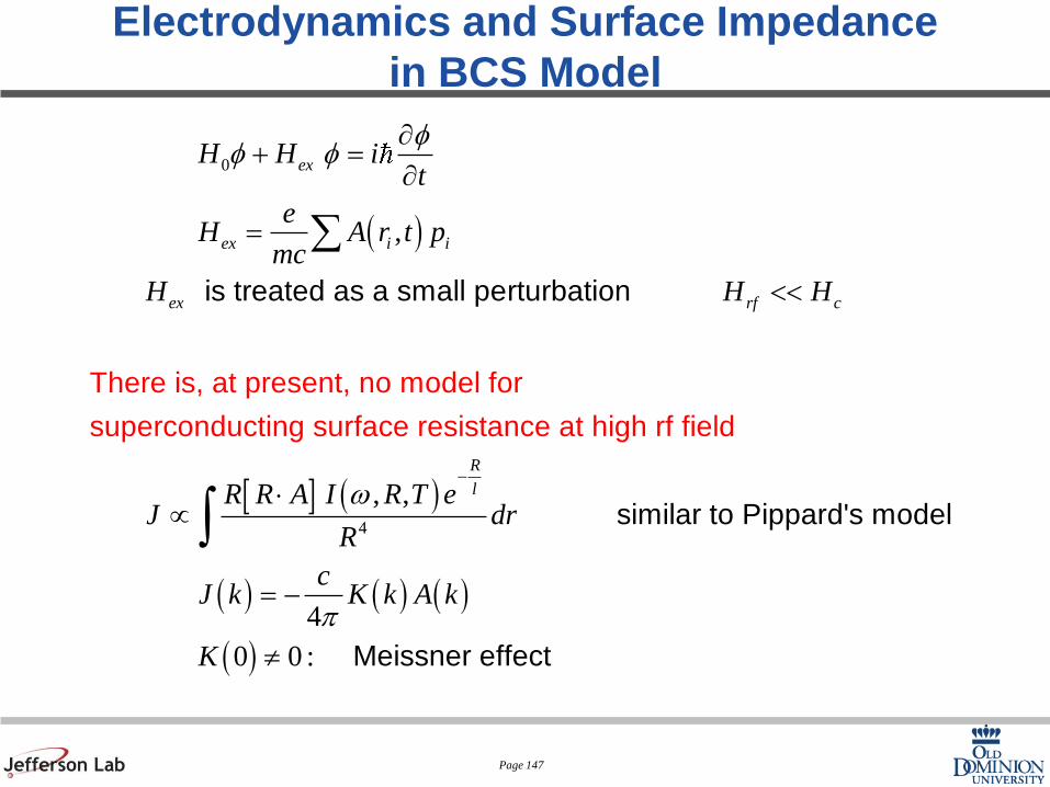
There is, at present, no model for superconducting
surface resistanc
is treated as a smal
e
l perturbation
at high rf fie
simil
ld
ar to
( ) ( ) ( )4
(0) 0 :
cJ k K k A k
K
p= -
¹
Pippard's model
Meissner effect

Page 127
Penetration Depth
2
4
2( )
( )
dkdk
K k k
TT
T
lp
l
=+
æ öç ÷è ø
ò
c
c
specular
1Represented accurately by near
1-

Page 128
Surface Resistance
( )4
32 2
2
:(1 )
:2
exp
-kT
2
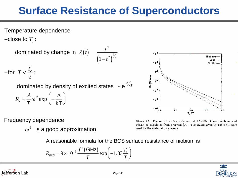
Temperature dependence
close to dominated by change in
for dominated by density of excited states e
Frequency dependence
is a good approximation
c
c
s
tT t
t
TT
AR
T kT
l
w
w
D
--
- <
Dæ ö-ç ÷è ø

Page 129
Surface Resistance

Page 130
Surface Resistance

Page 131
Surface Resistance

Page 132
Surface Impedance - Definitions
• The electromagnetic response of a metal,
whether normal or superconducting, is described
by a complex surface impedance, Z=R+iX
R : Surface resistance
X : Surface reactance
Both R and X are real

Page 133
Definitions
For a semi- infinite slab:
0
0
0
(0)
( )
(0) (0)
(0) ( ) /
Definition
From Maxwell
x
x
x x
y x z
EZ
J z dz
E Ei
H E z zw m
+
¥
=
=
= =¶ 
ò

Page 134
Definitions
The surface resistance is also related to the power flow
into the conductor
and to the power dissipated inside the conductor
212 (0 )P R H -=
( )0
0
0
1/2
0
(0 ) / (0 )
377 Impedance of vacuum
Poynting vector
Z Z S S
Z
S E H
m
e
+ -=
= W
= ´
Page 135
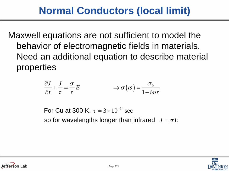
Normal Conductors (local limit)
Maxwell equations are not sufficient to model the
behavior of electromagnetic fields in materials.
Need an additional equation to describe material
properties
( ) 0
14
1
3 10 secFor Cu at 300 K,
so for wavelengths longer than infrared
J JE
t i
J E
sss w
t t wt
t
s
-
¶+ = Þ =
¶ -
= ´
=

Page 136
Normal Conductors (local limit)
In the local limit
The fields decay with a characteristic
length (skin depth)
( ) ( )J z E zs=
/ /
0
1/2
00
( ) (0)
(1 )( ) ( )
(0) (1 ) (1 )(1 )
(0) 2 2
z iz
x x
y x
x
y
E z E e e
iH z E z
E i iZ i
H
d d
m w d
m wm wd
s d s
- -=
-=
æ ö+ += = = = + ç ÷è ø
1/2
0
2d
m ws
æ ö= ç ÷è ø

Page 137
Normal Conductors (anomalous limit)
• At low temperature, experiments show that the surface
resistance becomes independent of the conductivity
• As the temperature decreases, the conductivity s increases
– The skin depth decreases
– The skin depth (the distance over which fields vary) can
become less then the mean free path of the electrons (the
distance they travel before being scattered)
– The electrons do not experience a constant electric field
over a mean free path
– The local relationship between field and current is not
valid ( ) ( )J z E zs¹
1/2
0
2d
m ws
æ ö= ç ÷è ø
Page 138
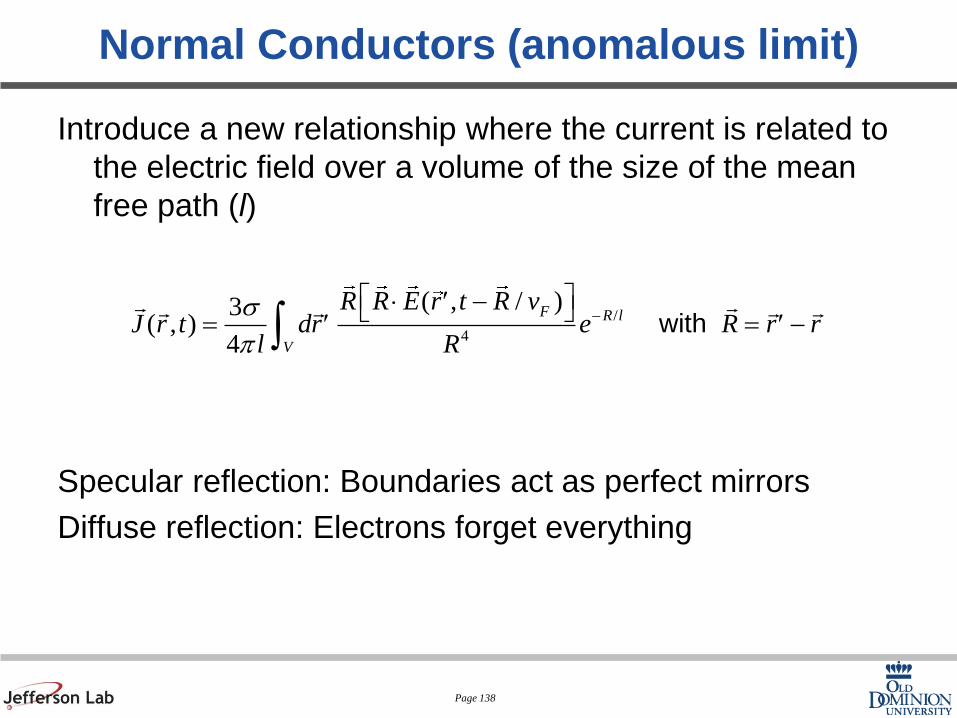
Normal Conductors (anomalous limit)
Introduce a new relationship where the current is related to
the electric field over a volume of the size of the mean
free path (l)
Specular reflection: Boundaries act as perfect mirrors
Diffuse reflection: Electrons forget everything
/
4
( , / )3( , )
4with
F R l
V
R R E r t R vJ r t dr e R r r
l R
s
p
-é ù× -¢ë û
= = -¢ ¢ò

Page 139
Normal Conductors (anomalous limit)
In the extreme anomalous limit
( )1/3
2 2
091 08
31 3
16
1 :
: fraction of electrons specularly scattered at surface
fraction of electrons diffusively scattered
p p
lZ Z i
p
p
m w
p s= =
æ ö= = +ç ÷
è ø
-
2
2
31
2 cl
l
d
æ öç ÷è ø
Page 140
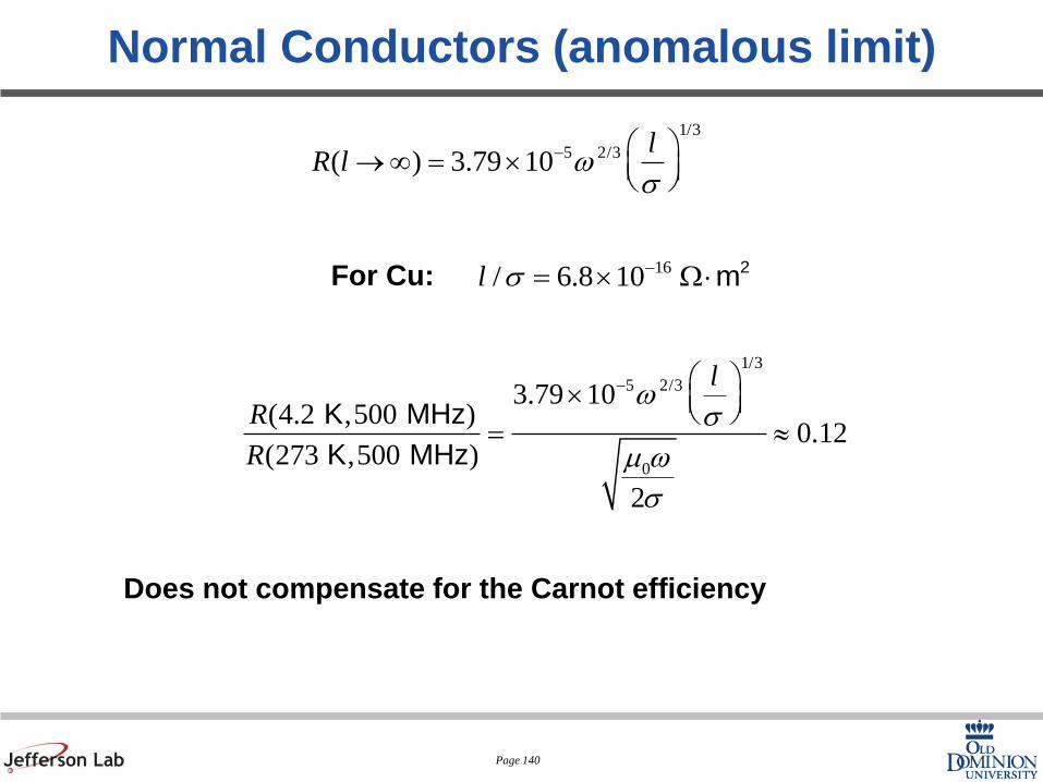
1/3
5 2/3( ) 3.79 10l
R l ws
- æ ö®¥ = ´ ç ÷è ø
For Cu: 16/ 6.8 10 2ml s -= ´ W×
1/3
5 2/3
0
3.79 10(4.2 ,500 )
0.12(273 ,500 )
2
K MHz
K MHz
l
R
R
ws
m w
s
- æ ö´ ç ÷è ø
= »
Does not compensate for the Carnot efficiency
Normal Conductors (anomalous limit)

Page 141
Surface Resistance of Superconductors
Superconductors are free of power dissipation in static fields.
In microwave fields, the time-dependent magnetic field in the
penetration depth will generate an electric field.
The electric field will induce oscillations in the normal
electrons, which will lead to power dissipation
BE
t
¶Ñ´ = -

Page 142
Surface Impedance in the Two-Fluid Model
In a superconductor, a time-dependent current will be carried
by the Copper pairs (superfluid component) and by the
unpaired electrons (normal component)
0
2
0 0
0
2
2
0
(
2( )
2 1
Ohm's law for normal electrons)
with
n s
i t
n n
i t i tcs e c
e
i t
cn s s
e L
J J J
J E e
n eJ i E e m v eE e
m
J E e
n ei
m
w
w w
w
s
w
s
s s s sw m l w
-
- -
-
= +
=
= = -
=
= + = =

Page 143
Surface Impedance in the Two-Fluid Model
For normal conductors 1sR
sd=
For superconductors
( ) 2 2 2
1 1 1n ns
L n s L n s L s
Ri
s s
l s s l s s l s
é ù= Â =ê ú
+ +ë û
The superconducting state surface resistance is proportional to the
normal state conductivity

Page 144
Surface Impedance in the Two-Fluid Model
2
2
2
0
3 2
1
( ) 1exp
( )exp
ns
L s
nn s
e F L
s L
R
n e l Tl
m v kT
TR l
kT
s
l s
s sm l w
l w
Dé ù= µ - =ê ú
ë û
Dé ùµ -ê ú
ë û
This assumes that the mean free path is much larger than the
coherence length
Page 145
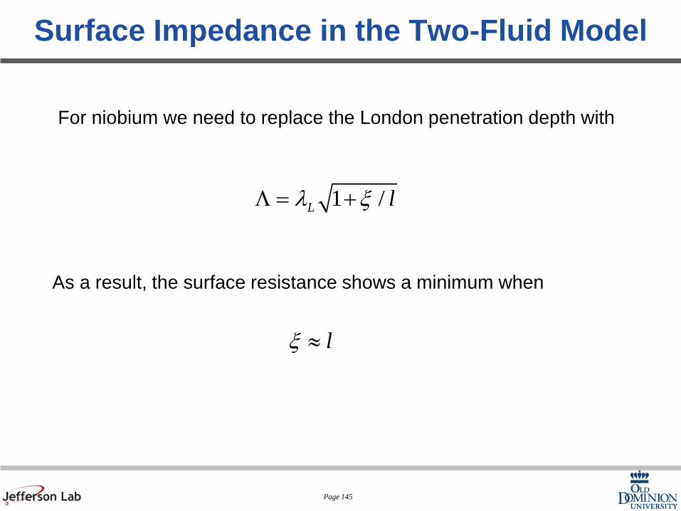
Surface Impedance in the Two-Fluid Model
For niobium we need to replace the London penetration depth with
1 /L ll xL = +
As a result, the surface resistance shows a minimum when
lx »

Page 146
Surface Resistance of Niobium
Surface Resistance - Nb - 1500 MHz
1
10
100
1000
10000
10 100 1000 10000
Mean Free Path (Angstrom)
nohm
2.0 K
4.0 K
4.2 K
3.5 K
3.0 K
2.5 K
1.8 K
Page 147
Electrodynamics and Surface Impedance
in BCS Model
( )
[ ] ( )
0
4
,
, ,
There is, at present, no model for
superconducting sur
is treated as a small pe
face resistance at high rf
rturbation
similar to Pippar
field
ex
ex i i
ex rf c
R
l
H H it
eH A r t p
mc
H H H
R R A I R T eJ dr
R
ff f
w-
¶+ =
=
<<
×µ
å
ò( ) ( ) ( )
( )4
0 0 :
d's model
Meissner effect
cJ k K k A k
K
p= -
¹
Page 148
Surface Resistance of Superconductors
( )( )
4
32 2
2
:
1
:2
exp
-kT
2
Temperature dependence
close to
dominated by change in
for
dominated by density of excited states e
kT
Frequency dependence
is a good approximation
c
c
s
T
tt
t
TT
AR
T
l
w
w
D
-
-
- <
Dæ ö-ç ÷è ø
( )2
59 10 exp 1.83
A reasonable formula for the BCS surface resistance of niobium is
GHzc
BCS
f TR
T T
- æ ö= ´ -ç ÷è ø

Page 149
Surface Resistance of Superconductors
• The surface resistance of superconductors depends on
the frequency, the temperature, and a few material
parameters
– Transition temperature
– Energy gap
– Coherence length
– Penetration depth
– Mean free path
• A good approximation for T<Tc/2 and ω<<Δ/h is
2 exps res
AR R
T kTw
Dæ ö- +ç ÷è ø

Page 150
Surface Resistance of Superconductors
2 exps res
AR R
T kTw
Dæ ö- +ç ÷è ø
In the dirty limit
In the clean limit
Rres:
Residual surface resistance
No clear temperature dependence
No clear frequency dependence
Depends on trapped flux, impurities, grain boundaries, …
1/2
0 BCSl R lx -µ
0 BCSl R lx µ
Page 151
Surface Resistance of Superconductors

Page 152
Surface Resistance of Niobium

Page 153
Surface Resistance of Niobium

Page 154
Super and Normal Conductors
• Normal Conductors
– Skin depth proportional to ω-1/2
– Surface resistance proportional to ω1/2 → 2/3
– Surface resistance independent of temperature (at low T)
– For Cu at 300K and 1 GHz, Rs=8.3 mΩ
• Superconductors
– Penetration depth independent of ω
– Surface resistance proportional to ω2
– Surface resistance strongly dependent of temperature
– For Nb at 2 K and 1 GHz, Rs≈7 nΩ
However: do not forget Carnot

Page 155
The Real World
11
10
9
8 0 25 50 MV/m
Accelerating Field
Residual losses
Multipacting
Field emission
Thermal breakdown
Quench
Ideal
RF Processing
10
10
10
10
Q

Page 156
Losses in SRF Cavities
• Different loss mechanism are associated with
different regions of the cavity surface
Electric field high at iris
Magnetic field high
at equator
Ep/Eacc ~ 2
Bp/Eacc ~ 4.2 mT/(MV/m)

Page 157
Characteristics of Residual Surface Resistance
• No strong temperature dependence
• No clear frequency dependence
• Not uniformly distributed (can be localized)
• Not reproducible
• Can be as low as 1 nΩ
• Usually between 5 and 30 nΩ
• Often reduced by UHV heat treatment above 800C

Page 158
Origin of Residual Surface Resistance
• Dielectric surface contaminants (gases, chemical
residues, dust, adsorbates)
• Normal conducting defects, inclusions
• Surface imperfections (cracks, scratches,
delaminations)
• Trapped magnetic flux
• Hydride precipitation
• Localized electron states in the oxide (photon
absorption)
Rres is typically 5-10 nW at 1-1.5 GHz

Page 159
Trapped Magnetic Field
A parallel magnetic filed is expelled from a
superconductor.
What about a perpendicular magnetic field?
The magnetic field will be concentrated in normal cores where it is
equal to the critical field.

Page 160
Trapped Magnetic Field
• Vortices are normal to the surface
• 100% flux trapping
• RF dissipation is due to the normal
conducting core, of resistance Rn
2
ires n
c
HR R
H Hi
= residual DC
magnetic field
• For Nb:
• While a cavity goes through the superconducting transition, the ambient
magnetic filed cannot be more than a few mG.
• The earth’s magnetic shield must be effectively shielded.
• Thermoelectric currents can cause trapped magnetic field, especially in
cavities made of composite materials.
0.3resR W to 1 n /mG around 1 GHzDepends on material treatment

Page 161
Trapped Magnetic Field
A fraction of the material will be in the normal state.
This will lead to an effective surface resistance
For Nb:
While a cavity goes through the superconducting transition, the ambient
magnetic filed cannot be more than a few mG.
The earth’s magnetic shield must be effectively shielded.
In cavities made of composite materials, thermoelectric currents can cause
trapped magnetic field.
/ cH H
( )/n cH Hr
0.5 to 1 n /mG around 1 GHzeffr » W

Page 162
Rres Due to Hydrides (Q-Disease)
• Cavities that remain at 70-150 K for several hours (or slow cool-down, < 1
K/min) experience a sharp increase of residual resistance
• More severe in cavities which have been heavily chemically etched

Page 163
Multipacting
• No increase of Pt for increased Pi during MP
• Can induce quenches and trigger field emission

Page 164
Multipacting
Multipacting is characterized by an exponential growth in the number of
electrons in a cavity
Common problems of RF structures (Power couplers, NC cavities…)
Multipacting requires 2 conditions:
• Electron motion is periodic (resonance condition)
• Impact energy is such that secondary emission coefficient is >1

Page 165
One-Point Multipacting
One-point MP
Cyclotron frequency:
Resonance condition:
Cavity frequency (g) = n x cyclotron
frequency
Possible MP barriers given by
n: MP
order
The impact energy scales as 2 2
2
g
e EK
m
+ SEY, d(K), > 1 = MP
Empirical formula: 0
0.3Oe MHznH f
n
Page 166
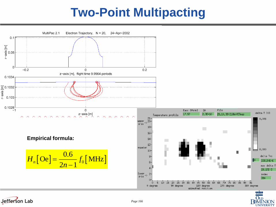
Two-Point Multipacting
Empirical formula:
0
0.6Oe MHz
2 1nH f
n

Page 167
Secondary Emission in Niobium

Page 168
Field Emission
• Characterized by an exponential drop of the Q0
• Associated with production of x-rays and emission of dark current
1.E+09
1.E+10
1.E+11
0 5 10 15 20
Qo
E (MV/m)
SNS HB54 Qo versus Eacc
0
0
0
0
1
10
100
1000
10000
0 5 10 15 20 25
mR
em
/hr)
E (MV/m)
SNS HTB 54 Radiation at top plate versus Eacc 5/16/08 cg
Page 169
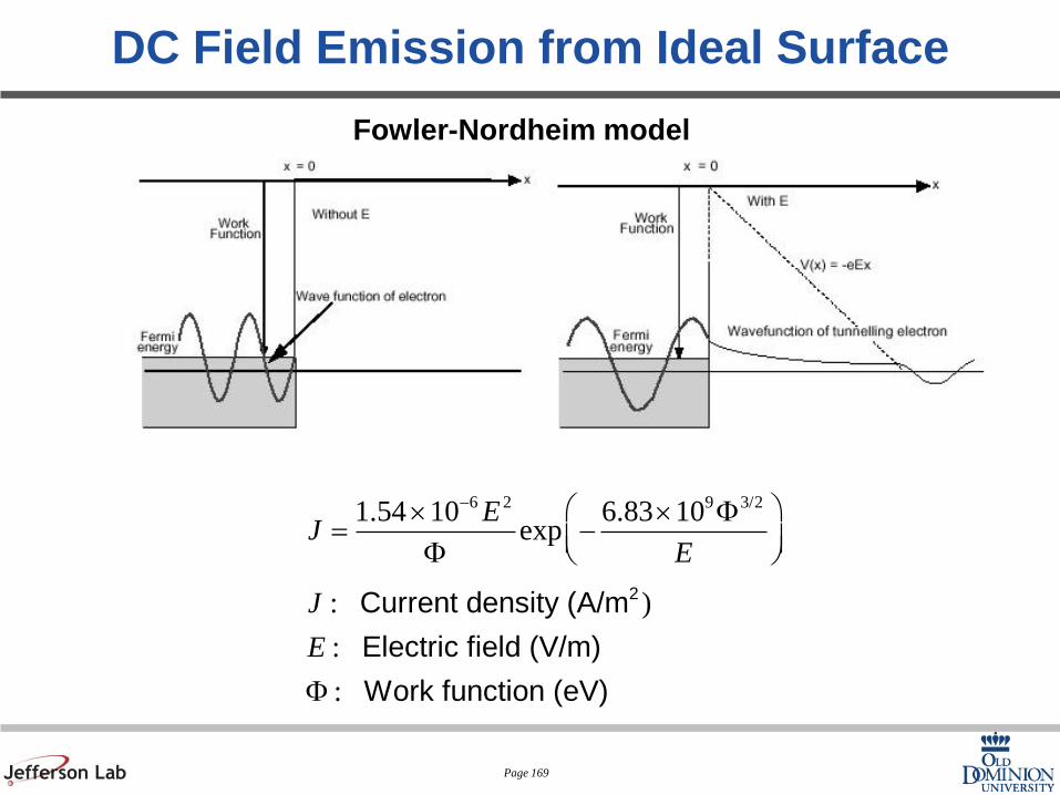
DC Field Emission from Ideal Surface
Fowler-Nordheim model
6 2 9 3/21.54 10 6.83 10exp
: )
:
:
2 Current density (A/m
Electric field (V/m)
Work function (eV)
EJ
E
J
E
- æ ö´ ´ F= -ç ÷F è ø
F

Page 170
Field Emission in RF Cavities
Acceleration of
electrons drains cavity
energy
Impacting electrons produce:
• line heating detected by
thermometry
• bremsstrahlung X rays
Foreign particulate
found at emission
site
FE in cavities occurs at fields that
are up to 1000 times lower than
predicted…
5/26 9 3/21.54 10 ( ) 6.83 10exp
:
:
Enhancement factor (10s to 100s)
Effective emitting surface
kE
JE
k
b
b
b
- æ ö´ ´ F= -ç ÷F è ø

Page 171
C, O, Na, In Al, Si
Stainless steel
Melted
Melted
Melted
Example of Field Emitters

Page 172
Type of Emitters
Smooth nickel particles emit
less or emit at higher fields.
Ni
V
•Tip-on-tip model
explains why only 10%
of particles are emitters
for Epk < 200 MV/m.
Page 173
Cures for Field Emission
• Prevention:
– Semiconductor grade acids and solvents
– High-Pressure Rinsing with ultra-pure water
– Clean-room assembly
– Simplified procedures and components for
assembly
– Clean vacuum systems (evacuation and venting
without re-contamination)
• Post-processing:
– Helium processing
– High Peak Power (HPP) processing

Page 174
Helium Processing
• Helium gas is introduced in the cavity at a pressure just
below breakdown (~10-5 torr)
• Cavity is operating at the highest field possible (in heavy
field emission regime)
• Duty cycle is adjusted to remain thermally stable
• Field emitted electrons ionized helium gas
• Helium ions stream back to emitting site
– Cleans surface contamination
– Sputters sharp protrusions
Page 175
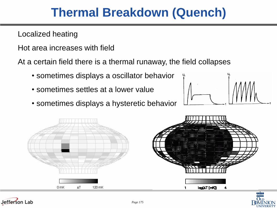
Thermal Breakdown (Quench)
Localized heating
Hot area increases with field
At a certain field there is a thermal runaway, the field collapses
• sometimes displays a oscillator behavior
• sometimes settles at a lower value
• sometimes displays a hysteretic behavior

Page 176
Thermal Breakdown
Thermal breakdown occurs when the heat generated at the hot spot is
larger than that can be transferred to the helium bath causing T > Tc:
“quench” of the superconducting state