Rewriting Schemes for Flash Memory

Thesis by

Eyal En Gad

In Partial Fulfillment of the Requirements

for the Degree of

Doctor of Philosophy

California Institute of Technology

Pasadena, California

2015

(Defended February 25, 2015)

ii

c© 2015

Eyal En Gad

All Rights Reserved

iii

To my mother

and

my wife Anna

iv

Acknowledgments

I would like to start by acknowledging my advisor Jehoshua (Shuki) Bruck, for his enormous

contributions to this thesis and to my professional and personal development during my time

at Caltech. Shuki’s advices about problem selection, motivation, solutions, and presentation

led me to enjoy my work greatly and to take pride in my results. He also taught me how

to be always optimistic and kind, and to enjoy fruitful collaborations. I feel very lucky and

grateful for having the opportunity to study under him.

During my graduate studies I was lucky to collaborate and learn from many other won-

derful researchers. Moshe Schwartz introduced me to the beauty and utility of combinatorial

coding theory, and taught me many useful ways to present research ideas. His sharp mind

and kind attitude were very inspiring for me. Michael Langberg taught me many concepts

in combinatorics and information theory with a very thorough approach. I also learned a lot

from him about how to explain research results in an interesting and clear way, and how to

always be kind and pleasant with everyone. Andrew Jiang introduced me to wonderful ideas

about coding in flash memory. His energy and excitement are contagious and make every

discussion with him very joyful. Joerg Kliewer introduced me to many concepts in modern

coding theory, and is always exited to explore new research directions. The discussions with

him gave me many exiting ideas and new perspectives.

I also had the opportunity to collaborate with several of my lab-mates at the Paradise

lab, which was a wonderful experience. I had a great time working with Eitan Yaakobi

during the two years he spent in the Paradise lab. He brought his endless optimism and

energy and his valuable experience in flash memory coding. Yue Li is a great collaborator

and friend since he joined the group. I am thankful for the practical perspective he gave

v

me towards research, and for his constant smile that kept the atmosphere in lab always

cheerful. I am also thankful for many challenging racquetball matches with him. Another

great collaborator and lab-mate is Wentao Huang, with whom I worked in the last part of

my studies. I am thankful to Wentao’s dedication and innovative thinking that made this

work very exiting.

I am also thankful to the many other lab members that I did not have the chance to

collaborate with: Daniel Wilhelm, Hongchao Zhou, Zhiying Wang, David Lee, Itzhak Tamo,

Lulu Qian, Farzad Farnoud, and Siddharth Jain.

I would like to thank Robert Mateescu, who hosted me in an internship at HGST. I had

a great time during the three months I spent at the Storage Architecture group. I am very

grateful to my collaborators at HGST - Filip Blagojevic, Cyril Guyot and Zvonimir Bandic

- and to the other friendly people at the research group, including Dejan Vucinic, Qingbo

Wang, Luiz Franca-Neto, and Jorge Campello.

I would like to thank my thesis committee: Michelle Effros, Babak Hassibi and P. P.

Vaidyanathan. Their illuminating questions and comments provided me with different points

of view and new ways of thinking.

I am very thankful for the remote support of my family and friends in Israel. My mother

Orna, my stepfather Uri, my brother Oded and my sister Neta. Your love and support was

an indispensable ingredient of the success and joy I had in my doctoral studies.

Finally, I was lucky to meet my wonderful and beautiful wife Anna during my time at

Caltech. This was the most successful part of my PhD effort. I am very grateful for her

love and partnership, which gave a new meaning to my work. I am also thankful for my

parents-in-law Manuel and Suzette and my sibling-in-law Sergio and Priscilla for making me

part of their family.

vi

Abstract

Flash memory is a leading storage media with excellent features such as random access and

high storage density. However, it also faces significant reliability and endurance challenges.

In flash memory, the charge level in the cells can be easily increased, but removing charge

requires an expensive erasure operation. In this thesis we study rewriting schemes that

enable the data stored in a set of cells to be rewritten by only increasing the charge level

in the cells. We consider two types of modulation scheme; a convectional modulation based

on the absolute levels of the cells, and a recently-proposed scheme based on the relative cell

levels, called rank modulation. The contributions of this thesis to the study of rewriting

schemes for rank modulation include the following: we

• propose a new method of rewriting in rank modulation, beyond the previously proposed

method of “push-to-the-top”;

• study the limits of rewriting with the newly proposed method, and derive a tight upper

bound of 1 bit per cell;

• extend the rank-modulation scheme to support rankings with repetitions, in order to

improve the storage density;

• derive a tight upper bound of 2 bits per cell for rewriting in rank modulation with

repetitions;

• construct an efficient rewriting scheme that asymptotically approaches the upper bound

of 2 bit per cell.

vii

The next part of this thesis studies rewriting schemes for a conventional absolute-levels

modulation. The considered model is called “write-once memory” (WOM). We focus on

WOM schemes that achieve the capacity of the model. In recent years several capacity-

achieving WOM schemes were proposed, based on polar codes and randomness extractors.

The contributions of this thesis to the study of WOM scheme include the following: we

• propose a new capacity-achieving WOM scheme based on sparse-graph codes, and show

its attractive properties for practical implementation;

• improve the design of polar WOM schemes to remove the reliance on shared randomness

and include an error-correction capability.

The last part of the thesis studies the local rank-modulation (LRM) scheme, in which a

sliding window going over a sequence of real-valued variables induces a sequence of permu-

tations. The LRM scheme is used to simulate a single conventional multi-level flash cell.

The simulated cell is realized by a Gray code traversing all the relative-value states where,

physically, the transition between two adjacent states in the Gray code is achieved by using

a single “push-to-the-top” operation. The main results of the last part of the thesis are two

constructions of Gray codes with asymptotically-optimal rate.

viii

Contents

Acknowledgments iv

Abstract vi

I Introduction 1

1 Rewriting in Flash Memory 2

1.1 Rank Modulation . . . . . . . . . . . . . . . . . . . . . . . . . . . . . . . . . 3

1.2 Write-Once Memory . . . . . . . . . . . . . . . . . . . . . . . . . . . . . . . 6

1.3 Local Rank Modulation . . . . . . . . . . . . . . . . . . . . . . . . . . . . . 8

II Rewriting with Rank Modulation 10

2 Model and Limits of Rewriting Schemes 11

2.1 Modifications to the Rank-Modulation Scheme . . . . . . . . . . . . . . . . . 11

2.2 Definition and Limits of Rank-Modulation Rewriting Codes . . . . . . . . . 16

2.3 Proof of the Cost Function . . . . . . . . . . . . . . . . . . . . . . . . . . . . 22

3 Efficient Rewriting Schemes 25

3.1 High-Level Construction . . . . . . . . . . . . . . . . . . . . . . . . . . . . . 25

3.2 Constant-Weight Polar WOM Codes . . . . . . . . . . . . . . . . . . . . . . 40

3.3 Rank-Modulation Schemes from Hash WOM Schemes . . . . . . . . . . . . . 47

ix

3.4 Summary . . . . . . . . . . . . . . . . . . . . . . . . . . . . . . . . . . . . . 53

3.5 Capacity Proofs . . . . . . . . . . . . . . . . . . . . . . . . . . . . . . . . . . 54

III Write-Once Memory 57

4 Rewriting with Sparse-Graph Codes 58

4.1 Rewriting and Erasure Quantization . . . . . . . . . . . . . . . . . . . . . . 58

4.2 Rewriting with Message Passing . . . . . . . . . . . . . . . . . . . . . . . . . 61

4.3 Error-Correcting Rewriting Codes . . . . . . . . . . . . . . . . . . . . . . . . 66

4.4 Summary . . . . . . . . . . . . . . . . . . . . . . . . . . . . . . . . . . . . . 71

5 Rewriting with Polar Codes 72

5.1 Relation to Previous Work . . . . . . . . . . . . . . . . . . . . . . . . . . . . 72

5.2 Asymmetric Point-to-Point Channels . . . . . . . . . . . . . . . . . . . . . . 74

5.3 Channels with Non-Causal Encoder State Information . . . . . . . . . . . . . 82

5.4 Summary . . . . . . . . . . . . . . . . . . . . . . . . . . . . . . . . . . . . . 93

5.5 Capacity Proofs . . . . . . . . . . . . . . . . . . . . . . . . . . . . . . . . . . 94

5.6 Proof of Theorem 5.7 . . . . . . . . . . . . . . . . . . . . . . . . . . . . . . . 100

IV Local Rank Modulation 109

6 Rewriting with Gray Codes 110

6.1 Definitions and Notation . . . . . . . . . . . . . . . . . . . . . . . . . . . . . 110

6.2 Constant-Weight Gray Codes for (1, 2, n)-LRM . . . . . . . . . . . . . . . . . 118

6.3 Gray Codes for (s, t, n)-LRM . . . . . . . . . . . . . . . . . . . . . . . . . . . 124

6.4 Summary . . . . . . . . . . . . . . . . . . . . . . . . . . . . . . . . . . . . . 139

Bibliography 140

x

List of Figures

3.1 Iteration i of the encoding algorithm, where 1 ≤ i ≤ q − r − 1. . . . . . . . . . 34

4.1 Rewriting failure rates of polar and LDGM WOM codes. . . . . . . . . . . . . 65

4.2 Encoding performance of the codes in Table 4.1. . . . . . . . . . . . . . . . . . 68

5.1 Encoding the vector u[n]. . . . . . . . . . . . . . . . . . . . . . . . . . . . . . . 77

5.2 Example 5.1: A binary noisy WOM model. . . . . . . . . . . . . . . . . . . . 85

5.3 Example 5.2: A binary WOM with writing noise. . . . . . . . . . . . . . . . . 86

5.4 Encoding the vector u[n] in Construction 5.2. . . . . . . . . . . . . . . . . . . 88

5.5 The chaining construction . . . . . . . . . . . . . . . . . . . . . . . . . . . . . 91

6.1 Demodulating a (3, 5, 12)-locally rank-modulated signal. . . . . . . . . . . . . 111

6.2 A “push-to-the-top” operation performed on the 9th cell. . . . . . . . . . . . . 114

xi

List of Tables

1.1 WOM-Code Example . . . . . . . . . . . . . . . . . . . . . . . . . . . . . . . 3

4.1 Error-correcting Rewriting Codes from Conjugate Pairs . . . . . . . . . . . . . 68

4.2 Error-correcting rewriting codes of length ≈ 8200. . . . . . . . . . . . . . . . . 71

6.1 A cyclic optimal (1, 2, 5; 2)-LRMGC . . . . . . . . . . . . . . . . . . . . . . . 117

6.2 The transitions between anchors in Example 6.1. . . . . . . . . . . . . . . . . 122

1

Part I

Introduction

2

Chapter 1

Rewriting in Flash Memory

This thesis deals with coding schemes for data storage in flash memory. Flash memory is a

leading storage media with many excellent features such as random access and high storage

density. However, it also faces significant reliability and endurance challenges. Flash memory

contains floating gate cells. The cells are electrically charged with electrons and can represent

multiple levels according to the number of electrons they contain. The most conspicuous

property of flash-storage technology is its inherent asymmetry between cell programming

and cell erasing. While it is fast and simple to increase a cell level, reducing its level requires

a long and cumbersome operation of first erasing its entire containing block (∼ 106cells)

and only then programming the cells [8]. Such block erasures are not only time consuming,

but also degrade the lifetime of the memory. A typical block can generally tolerate at most

104 − 105 erasures.

To reduce the amount of block erasures, the focus of this thesis is on schemes for the

rewriting of data in the memory. Rewriting schemes allow to update information stored in a

set of flash cells solely by increasing the cell levels (without decreasing the level of any cell).

Rewriting schemes were in fact studied before the emergence of flash memory, as memories

whose cells transit irreversibly between states have been common since the beginning of the

data storage technology. Examples include punch cards and digital optical discs, where a cell

can change from a 0-state to a 1-state but not vice versa. In addition, non-volatile memories

other than flash memory also exhibit an asymmetric writing property, such as phase-change

3

Table 1.1: WOM-Code ExampleData bits First write Second write (if data changes)

00 000 11110 100 01101 010 10111 001 110

memories.

The first example of a rewriting scheme was given by Rivest and Shamir in 1982 [69].

This example considers a rewriting model called write-once memory (WOM), in which the

memory cells take binary values, and can only change for 0 to 1. The example is a simple

WOM code that enables the recording of two bits of information in three memory cells

twice. The encoding and decoding rules for this WOM-code are described in a tabular form

in Table 1.1. It is easy to verify that after the first 2-bit data vector is encoded into a 3-bit

codeword, if the second 2-bit data vector is different from the first, the 3-bit codeword into

which it is encoded does not change any code bit 1 into a code bit 0, ensuring that it can be

recorded in the write-once medium.

WOM codes with more cells and more data bits were studied extensively in recent years,

since the emergence of the flash memory application. In this thesis we make several contri-

bution to the study of WOM codes. In addition to WOM, the thesis also studies rewriting

in a different data-representation scheme, called rank modulation. We turn our attention

now to describe the rewriting setting in rank modulation.

1.1 Rank Modulation

Rank modulation was recently proposed [45]. In this scheme a set of n memory cells repre-

sents information according to the ranking of the cell levels. For example, we can use a set

of 3 cells, labeled from 1 to 3, such that each cell has a distinct charge level. We then rank

the cells according to their charge levels, and obtain one of 3! = 6 possible permutations over

the set {1, 2, 3}. A possible ranking would be, for example, cell 3 with the highest level, then

4

cell 1 and then cell 2 with the lowest level. Each ranking can represent a distinct information

message, and so the 3 cells in this example store together log2 6 bits. It was suggested in [45]

that the rank-modulation scheme speeds up data writing by eliminating the over-shooting

problem in flash memories. In addition, it also increases the data retention by mitigating

the effect of charge leakage.

Rank-modulation rewriting codes were proposed in [45, Section IV], with respect to a

rewriting method called “push-to-the-top”. In this rewriting method, the charge level of a

single cell is pushed up to be higher than that of any other cell in the ranking. In other words,

a push-to-the-top operation changes the rank of a single cell to be the highest. A rewriting

operation involves a sequence of push-to-the-top operations that transforms the cell ranking

to represent a desired updated data. The cells, however, have an upper limit on their possible

charge levels. Therefore, after a certain number of rewriting operations, the user must resort

to the expensive erasure operation in order to continue updating the memory. The concept

of rewriting codes was proposed in order to control the trade-off between the number of data

updates and the amount of data stored in each update. Note that the number of performed

push-to-the-top operations determines when an expensive block erasure is required. However,

the number of rewriting operations itself does not affect the triggering of the block erasure.

Therefore, rewriting operations that require fewer push-to-the-top operations can be seen

as cheaper, and are therefore more desirable. Nevertheless, limiting the memory to cheap

rewriting operations would reduce the number of potential rankings to write, and therefore

would reduce the amount of information that could be stored. We refer to the number of

push-to-the-top operations in a given rewriting operation as the cost of rewriting. The study

in [45, Section IV] considers rewriting codes with a constrained rewriting cost.

We study rank-modulation in Part II of the thesis. The first contribution of this part is

a modification of the framework of rank-modulation rewriting codes, in two ways. First, we

modify the rank-modulation scheme to allow rankings with repetitions, meaning that multiple

cells can share the same rank, where the number of cells in each rank is predetermined. And

second, we extend the rewriting operation to allow pushing a cell’s level above that of any

5

desired cell, instead of only above the level of the top cell. We justify both modifications

and devise an appropriate notion of rewriting cost. Specifically, we define the cost to be the

difference between the charge level of the highest cell, after the writing operation, to the

charge level of the highest cell before the rewriting operation. We suggest and explain why

the new cost function compares fairly to that of the push-to-the-top model. We then go on

to study rewriting codes in the modified framework.

We measure the storage rate of rewriting codes by the ratio between the number of stored

information bits in each write, to the number of cells in the ranking. We study the case in

which the number of cells is large (and asymptotically growing), while the cost constraint

is a constant, as this case appears to be fairly relevant for practical applications. In the

model of push-to-the-top rewriting which was studied in [45, Section IV], the storage rate

vanishes when the number of cells grows. Our first interesting result is that the asymptotic

storage rate in our modified framework converges into a positive value (that depends on

the cost constraint). Specifically, using rankings without repetitions, i.e. the original rank

modulation scheme with the modified rewriting operation, and the minimal cost constraint

of a single unit, the best storage rate converges to a value of 1 bit per cell. Moreover, when

ranking with repetitions is allowed, the best storage rate with a minimal cost constraint

converges to a value of 2 bits per cell.

Motivated by these positive results, we design an explicit construction of rank-modulation

rewriting codes, together with computationally efficient encoding and decoding algorithms.

The main ingredients in the code construction are write-once memory (WOM) schemes. We

focus on ranking with repetitions, where both the number of cells in each rank and the

number of ranks are growing. In this case, we show how to make use of capacity-achieving

WOM codes to construct rank-modulation rewriting codes with an asymptotically optimal

rate for any given cost constraint.

6

1.2 Write-Once Memory

In Part III of this thesis we propose two new constructions of WOM codes. These construc-

tions can be used with an absolute-level modulation, or with the rank-modulation rewriting

schemes proposed in Part II.

The constructions proposed in this thesis are based on sparse-graph codes and on polar

codes. Sparse-graph WOM codes are introduced in this thesis, while polar WOM codes were

discovered earlier (in [7]), and this thesis contributes to their study. Many other types of

WOM codes were proposed in the literature, including [21,25,43,44,86,88,91].

An important feature of both WOM schemes proposed in this thesis is that they achieve

the capacity of the WOM model (given in [36]). The sparse-graph WOM codes achieve the

capacity of the WOM for two writes, while the polar WOM codes achieve the capacity for

any number of writes. In both schemes we also propose methods to integrate the WOM

codes with error-correcting codes.

1.2.1 Sparse-Graph WOM codes

The sparse-graph WOM codes are proposed for the case of two writes. The construction is

based on binary erasure quantization with low-density-generator-matrix (LDGM) codes. The

encoding is performed by the iterative quantization studied by Martinian and Yedidia [58],

which is a message-passing algorithm similar to the decoding of low-density-parity-check

(LDPC) codes. As LDPC codes have been widely adopted by commercial flash memory con-

trollers, the hardware architectures of message-passing algorithms have been well understood

and highly optimized in practice. Therefore, the proposed codes are implementation-friendly

for practitioners. Extensive simulations show that the rewriting performance of the scheme

compares favorably with that of the polar WOM code in the rate region where a low rewrit-

ing failure rate is desired. For instance, we show that our code allows user to write 40%

more information by rewriting with very high success probability. We note that the iter-

ative quantization algorithm of [58] was used in [10] in a different way for the problem of

7

information embedding, which shares some similarity with our model.

Moreover, the proposed construction is extended with error correction. We use conjugate

code pairs studied in the context of quantum error correction [35]. As an example, we

construct LDGM WOM codes whose codewords also belong to BCH codes. Therefore, our

codes allow to use any decoding algorithm of BCH codes. The latter have been implemented

in most commercial flash memory controllers. We also present two additional approaches to

add error correction, and compare their performance.

1.2.2 Polar WOM codes

Polar WOM codes were introduced in [7]. The construction is based on polar lossy source

codes of Korada and Urbanke [50], which are based on the polar channel codes of Arikan [1].

We propose a different construction of polar WOM codes, which offers two main advantages

over the previously proposed codes. First, our codes do not require shared randomness

between the encoder and decoder, which is required in the original polar WOM codes. And

second, we extend the codes with error correction capability.

The proposed polar codes are analyzed with respect to the model of channel coding

with state information available at the encoder, proposed by Gelfand and Pinsker [16, page

178] [28]. This model can be seen as a generalization of the model of point-to-point channel

coding model. This implies that the proposed coding scheme can be used also for point-

to-point channel coding. In this setting our schemes provides an additional contribution,

since it possesses favorable properties compared with known capacity-achieving schemes for

asymmetric point-to-point channels.

We consider two noisy WOM models, and provide two variations of the polar WOM

scheme. We show that each of these variations achieves the capacity of the respected noise

model.

8

1.3 Local Rank Modulation

In Part IV we consider a different approach to rewriting in the rank-modulation scheme.

The considered rewriting approach, described first in [45], is the following: a set of n cells,

over which the rank-modulation scheme is applied (without repetitions), is used to simu-

late a single conventional multi-level flash cell with n! levels corresponding to the alphabet

{0, 1, . . . , n!− 1}. The simulated cell supports an operation which raises its value by 1 mod-

ulo n!. This is the only required operation in many rewriting schemes for flash memories

(see [42, 43, 87]), and it is realized in [45] by a Gray code traversing the n! states where,

physically, the transition between two adjacent states in the Gray code is achieved by using

a single “push-to-the-top” operation.

Most generally, a gray code is a sequence of distinct elements from an ambient space such

that adjacent elements in the sequence are “similar”. Ever since their original publication

by Gray [33], the use of Gray codes has reached a wide variety of areas, such as storage and

retrieval applications [11], processor allocation [12], statistics [14], hashing [23], puzzles [27],

ordering documents [53], signal encoding [54], data compression [68], circuit testing [70], and

more.

The Gray code was first introduced as a sequence of distinct binary vectors of fixed length,

where every adjacent pair differs in a single coordinate [33]. It has since been generalized to

sequences of distinct states s1, s2, . . . , sk ∈ S such that for every i < k there exists a function

in a predetermined set of transitions τ ∈ T such that si+1 = τ(si) (see [77] for an excellent

survey). In the context of rank modulation in [45], the state space consisted of permutations

over n elements, and the “push-to-the-top” operations were the allowed transitions. This

operation was studied since it is a simple programming operation that is quick and eliminates

the over-programming problem. We also note that generating permutations using “push-

to-the-top” operations is of independent interest, called “nested cycling” in [78] (see also

references therein), motivated by a fast “push-to-the-top” operation (cycling) available on

some computer architectures.

A drawback to the rank-modulation scheme (without repetitions) is the need for a large

9

number of comparisons when reading the induced permutation from a set of n cell-charge

levels. Instead, in a recent work [85], the n cells are locally viewed through a sliding window,

resulting in a sequence of small permutations that require less comparisons. We call this the

local rank-modulation scheme. The aim of this part of the thesis is to study Gray codes for the

local rank-modulation scheme. Another generalization of Gray codes for rank modulation is

the “snake-in-the-box” codes in [89].

We present two constructions of asymptotically rate-optimal Gray codes. The first con-

struction considers the case of (1, 2, n)-LRMGC, while the second construction considers

the more general case of (s, t, n)-LRMGC. However, the first construction also considers an

additional property, in which the codes have a constant weight.

10

Part II

Rewriting with Rank Modulation

11

Chapter 2

Model and Limits of Rewriting

Schemes

The material in Chapters 2 and 3 was presented in part in [17, 18,22].

2.1 Modifications to the Rank-Modulation Scheme

In this section we motivate and define the rank-modulation scheme, together with the pro-

posed modification to the scheme and to the rewriting process.

2.1.1 Motivation for Rank Modulation

The rank-modulation scheme is motivated by the physical and architectural properties of

flash memories (and similar non-volatile memories). First, the charge injection in flash

memories is a noisy process in which an overshooting may occur. When the cells represent

data by their absolute value, such overshooting results in a different stored data than the

desired one. And since the cell level cannot be decreased, the charge injection is typically

performed iteratively and therefore slowly, to avoid such errors. However, in rank modulation

such overshooting errors can be corrected without decreasing the cell levels, by pushing other

cells to form the desired ranking. An additional issue in flash memories is the leakage of

charge from the cells over time, which introduces additional errors. In rank modulation, such

leakage is significantly less problematic, since it behaves similarly in spatially close cells, and

12

thus is not likely to change the cells’ ranking. A hardware implementation of the scheme

was recently designed on flash memories [47].

We note that the motivation above is valid also for the case of ranking with repetitions,

which was not considered in previous literature with respect to the rank-modulation scheme.

We also note that the rank-modulation scheme in some sense reduces the amount of infor-

mation that can be stored, since it limits the possible state that the cells can take. For

example, it is not allowed for all the cell levels to be the same. However, this disadvantage

might be worth taking for the benefits of rank modulation, and this is the case in which we

are interested in this part of the thesis.

2.1.2 Representing Data by Rankings with Repetitions

In this subsection we extend the rank-modulation scheme to allow rankings with repetitions,

and formally define the extended demodulation process. We refer to rankings with repetitions

as permutations of multisets, where rankings without repetitions are permutations of sets.

Let M = {az11 , . . . , azqq } be a multiset of q distinct elements, where each element ai appears zi

times. The positive integer zi is called the multiplicity of the element ai, and the cardinality

of the multiset is n =∑q

i=1 zi. For a positive integer n, the set {1, 2, . . . , n} is labeled

by [n]. We think of a permutation σ of the multiset M as a partition of the set [n] into

q disjoint subsets, σ = (σ(1), σ(2), . . . , σ(q)), such that |σ(i)| = zi for each i ∈ [q], and

∪i∈[q]σ(i) = [n]. We also define the inverse permutation σ−1 such that for each i ∈ [q] and

j ∈ [n], σ−1(j) = i if j is a member of the subset σ(i). We label σ−1 as the length-n vector

σ−1 = (σ−1(1), σ−1(2), . . . , σ−1(n)). For example, if M = {1, 1, 2, 2} and σ = ({1, 3} , {2, 4}),then σ−1 = (1, 2, 1, 2). We refer to both σ and σ−1 as a permutation, since they represent

the same object.

Let SM be the set of all permutations of the multiset M . By abuse of notation, we view

SM also as the set of the inverse permutations of the multiset M . For a given cardinality

n and number of elements q, it is easy to show that the number of multiset permutations is

maximized if the multiplicities of all of the elements are equal. Therefore, to simplify the pre-

13

sentation, we take most of the multisets in this thesis to be of the form M = {1z, 2z, . . . , qz},and label the set SM by Sq,z.

Consider a set of n memory cells, and denote x = (x1, x2, . . . , xn) ∈ Rn as the cell-state

vector. The values of the cells represent voltage levels, but we do not pay attention to

the units of these values (i.e., Volt). We represent information on the cells according to the

mutiset permutation that their values induce. This permutation is derived by a demodulation

process.

Demodulation: Given positive integers q and z, a cell-state vector x of length n = qz

is demodulated into a permutation π−1x

= (π−1x(1), π−1

x(2), . . . , π−1

x(n)). Note that while π−1

x

is a function of q, z and x, q and z are not specified in the notation since they will be clear

from the context. The demodulation is performed as follows: first, let k1, . . . , kn be an order

of the cells such that xk1 ≤ xk2 ≤ · · · ≤ xkn . Then, for each j ∈ [n], assign π−1x(kj) = ⌈j/z⌉.

Example 2.1: Let q = 3, z = 2 and so n = qz = 6. Assume that we wish to demodulate the

cell-state vector x = (1, 1.5, 0.3, 0.5, 2, 0.3). We first order the cells according to their values:

(k1, k2, . . . , k6) = (3, 6, 4, 1, 2, 5), since the third and sixth cells have the smallest value, and

so on. Then we assign

π−1x(k1 = 3) = ⌈1/2⌉ = 1,

π−1x(k2 = 6) = ⌈2/2⌉ = 1,

π−1x(k3 = 4) = ⌈3/2⌉ = 2,

and so on, and get the permutation π−1x

= (2, 3, 1, 2, 3, 1). Note that π−1x

is in S3,2.

Note that πx is not unique if for some i ∈ [q], xkzi = xkzi+1. In this case, we define

πx to be illegal and denote πx = F . We label QM as the set of all cell-state vectors that

demodulate into a valid permutation of M . That is, QM = {x ∈ Rn |πx 6= F}. So for all

x ∈ QM and i ∈ [q], we have xkzi < xkzi+1. For j ∈ [n], the value π−1(j) is called the rank of

cell j in the permutation π.

14

2.1.3 Rewriting in Rank Modulation

In this subsection we extend the rewriting operation in the rank-modulation scheme. Pre-

vious work considered a writing operation called “push-to-the-top”, in which a certain cell

is pushed to be the highest in the ranking [45]. Here we suggest to allow to push a cell

to be higher than the level of any specific other cell. We note that this operation is still

resilient to overshooting errors, and therefore benefits from the advantage of fast writing, as

the push-to-the-top operations.

We model the flash memory such that when a user wishes to store a message on the

memory, the cell levels can only increase. When the cells reach their maximal levels, an

expensive erasure operation is required. Therefore, in order to maximize the number of

writes between erasures, it is desirable to raise the cell levels as little as possible on each

write. For a cell-state vector x ∈ QM , denote by Γx(i) the highest level among the cells with

rank i in πx. That is,

Γx(i) = maxj∈πx(i)

{xj}.

Let s be the cell-state vector of the memory before the writing process takes place, and let

x be the cell-state vector after the write. In order to reduce the possibility of error in the

demodulation process, a certain gap must be placed between the levels of cells with different

ranks. Since the cell levels’s units are somewhat arbitrary, we set this gap to be the value 1,

for convenience. The following modulation method minimizes the increase in the cell levels.

Modulation: Writing a permutation π on a memory with state s. The output is the

new memory state, denoted by x.

1. For each j ∈ π(1), assign xj ⇐ sj.

2. For i = 2, 3, . . . , q, for each j ∈ π(i), assign

xj ⇐ max{sj,Γx(i− 1) + 1}.

15

Example 2.2: Let q = 3, z = 2 and so n = qz = 6. Let the state be

s = (2.7, 4, 1.5, 2.5, 3.8, 0.5) and the target permutation be π−1 = (1, 1, 2, 2, 3, 3). In step 1 of

the modulation process, we notice that π(1) = {1, 2}, and so we set

x1 ⇐ s1 = 2.7

and

x2 ⇐ s2 = 4.

In step 2 we have π(2) = {3, 4} and Γx(1) = max {x1, x2} = max {2.7, 4} = 4, so we set

x3 ⇐ max {s3,Γx(1) + 1} = max {1.5, 5} = 5

and

x4 ⇐ max {s4,Γx(1) + 1} = max {2.5, 5} = 5.

And in the last step we have π(3) = {5, 6} and Γx(2) = 5, so we set

x5 ⇐ max {3.8, 6} = 6

and

x6 ⇐ max {0.5, 6} = 6.

In summary, we get x = (2.7, 4, 5, 5, 6, 6), which demodulates into π−1x

= (1, 1, 2, 2, 3, 3) =

π−1, as required.

Since the cell levels cannot decrease, we must have xj ≥ sj for each j ∈ [n]. In addition,

for each j1 and j2 in [n] for which π−1(j1) > π−1(j2), we must have xj1 > xj2 . Therefore, the

proposed modulation process minimizes the increase in the levels of all the cells.

16

2.2 Definition and Limits of Rank-Modulation Rewrit-

ing Codes

Remember that the level xj of each cell is upper bounded by a certain value. Therefore, given

a state s, certain permutations π might require a block erasure before writing, while others

might not. In addition, some permutations might get the memory state closer to a state in

which an erasure is required than other permutations. In order to maximize the number of

writes between block erasures, we add redundancy by lettingmultiple permutations represent

the same information message. This way, when a user wishes to store a certain message,

she could choose one of the permutations that represent the required message such that the

chosen permutation will increase the cell levels in the least amount. Such a method can

increase the longevity of the memory in the expense of the amount of information stored

on each write. The mapping between the permutations and the messages they represent is

called a rewriting code.

To analyze and design rewriting codes, we focus on the difference between Γx(q) and

Γs(q). Using the modulation process we defined above, the vector x is a function of s and

π, and therefore the difference Γx(q) − Γs(q) is also a function of s and π. We label this

difference by α(s → π) = Γx(q) − Γs(q) and call it the rewriting cost, or simply the cost.

We motivate this choice by the following example. Assume that the difference between the

maximum level of the cells and Γs(q) is 10 levels. Then only the permutations π which

satisfy α(s → π) ≤ 10 can be written to the memory without erasure. Alternatively, if we

use a rewriting code that guarantees that for any state s, any message can be stored with,

say, cost no greater than 1, then we can guarantee to write 10 more times to the memory

before an erasure will be required. Such rewriting codes are the focus of this part of the

thesis.

The cost α(s → π) is defined according to the vectors s and x. However, it will be

helpful for the study of rewriting codes to have some understanding of the cost in terms of

the demodulation of the state s and the permutation π. To establish such connection, we

17

assume that the state s is a result of a previous modulation process. This assumption is

reasonable, since we are interested in the scenario of multiple successive rewriting operations.

In this case, for each i ∈ [q− 1], Γs(i+1)−Γs(i) ≥ 1, by the modulation process. Let σs be

the permutation obtained from the demodulation of the state s. We present the connection

in the following proposition.

Proposition 2.1: Let M be a multiset of cardinality n. If Γs(i + 1) − Γs(i) ≥ 1 for all

i ∈ [q − 1], and π is in SM , then

α(s→ π) ≤ maxj∈[n]{σ−1

s(j)− π−1(j)} (2.1)

with equality if Γq(s)− Γ1(s) = q − 1.

The proof of Proposition 2.1 is brought in Section 2.3. We would take a worst-case ap-

proach, and opt to design codes that guarantee that on each rewriting, the value maxj∈[n]{σ−1s(j)−

π−1(j)} is bounded. For permutations σ and π inSq,z, the rewriting cost α(σ → π) is defined

as

α(σ → π) = maxj∈[n]{σ−1(j)− π−1(j)}. (2.2)

This expression is an asymmetric version of the Chebyshev distance (also known as the L∞

distance). For simplicity, we assume that the channel is noiseless and don’t consider the

error-correction capability of the codes. However, such consideration would be essential for

practical applications.

2.2.1 Definition of Rank-Modulation Rewriting Codes

A rank-modulation rewriting code is a partition of the set of multiset permutations, such

that each part represents a different information message, and each message can be written

on each state with a cost that is bounded by some parameter r. A formal definition follows.

Definition 2.1: (Rank-modulation rewriting codes) Let q, z, r, and KR be positive

integers, and let C be a subset of Sq,z called the codebook. Then a surjective function DR :

18

C → [KR] is a (q, z,KR, r) rank-modulation rewriting code (RM rewriting code) if

for each message m ∈ [KR] and state σ ∈ C, there exists a permutation π in D−1R (m) ⊆ C

such that α(σ → π) ≤ r.

D−1R (m) is the set of permutations that represent the message m. It could also be in-

sightful to study rewriting codes according to an average cost constraint, assuming some

distribution on the source and/or the state. However, we use the wort-case constraint since

it is easier to analyze. The amount of information stored with a (q, z,KR, r) RM rewriting

code is logKR bits (all of the logarithms in this thesis are binary). Since it is possible to

store up to log |Sq,z| bits with permutations of a multiset {1z, . . . , qz}, it could be natural

to define the code rate as:

R′ =logKR

log |Sq,z|.

However, this definition doesn’t give much engineering insight into the amount of information

stored in a set of memory cells. Therefore, we define the rate of the code as the amount of

information stored per memory cell:

R =logKR

qz.

An encoding function ER for a code DR maps each pair of message m and state σ into a

permutation π such that DR(π) = m and α(σ → π) ≤ r. By abuse of notation, let the

symbols ER and DR represent both the functions and the algorithms that compute those

functions. If DR is a RM rewriting code and ER is its associated encoding function, we call

the pair (ER, DR) a rank-modulation rewrite coding scheme.

Rank-modulation rewriting codes were proposed by Jiang et al. in [45], in a more re-

strictive model than the one we defined above. The model in [45] is more restrictive in two

senses. First, the mentioned model used the rank-modulation scheme with permutations of

sets only, while here we also consider permutations of multisets. And second, the rewrit-

ing operation in the mentioned model was composed only of a cell programming operation

called “push-to-the-top”, while here we allow a more opportunistic programming approach.

19

A push-to-the-top operation raises the charge level of a single cell above the rest of the cells

in the set. As described above, the model of this chapter allows one to raise a cell level

above a subset of the rest of the cells. The rate of RM rewriting codes with push-to-the-top

operations and cost of r = 1 tends to zero with the increase in the block length n. On the

contrary, we will show that the rate of RM rewriting codes with cost r = 1 and the model

of this chapter tends to 1 bit per cell with permutations of sets, and 2 bits per cell with

permutations of multisets.

2.2.2 Limits of Rank-Modulation Rewriting Codes

For the purpose of studying the limits of RM rewriting codes, we define the ball of radius r

around a permutation σ in Sq,z by

Bq,z,r(σ) = {π ∈ Sq,z|α(σ → π) ≤ r},

and derive its size in the following lemma.

Lemma 2.1: For positive integers q and z, if σ is in Sq,z then

|Bq,z,r(σ)| =(

(r + 1)z

z

)q−r r∏

i=1

(

iz

z

)

.

Proof: Let π ∈ Bq,z,r(σ). By the definition ofBq,z,r(σ), for any j ∈ π(1), σ−1(j)−1 ≤ r, and

thus σ−1(j) ≤ r + 1. Therefore, there are(

(r+1)zz

)

possibilities for the set π(1) of cardinality

z. Similarly, for any i ∈ π(2), σ(i)−1 ≤ r + 2. So for each fixed set π(1), there are(

(r+1)zz

)

possibilities for π(2), and in total(

(r+1)zz

)2possibilities for the pair of sets (π(1), π(2)). The

same argument follows for all i ∈ [q − r], so there are(

(r+1)zz

)q−rpossibilities for the sets

(π(1), . . . , π(q − r)). The rest of the sets of π: π(q − r + 1), π(q − r + 2), . . . , π(q), can take

any permutation of the multiset {(q − r + 1)z, (q − r + 2)z, . . . , qz}, giving the statement of

the lemma. �

20

Note that the size of Bq,z,r(σ) is actually not a function of σ. Therefore we denote it by

|Bq,z,r|.

Proposition 2.2: Let DR be a (q, z,KR, r) RM rewriting code. Then

KR ≤ |Bq,z,r|.

Proof: Fix a state σ ∈ C. By Definition 2.1 of RM rewriting codes, for any message

m ∈ [KR] there exists a permutation π such that DR(π) = m and π is in Bq,z,r(σ). It follows

that Bq,z,r(σ) must contain KR different permutations, and so its size must be at least KR.�

Corollary 2.1: Let R(r) be the rate of an (q, z,KR, r)-RM rewriting code. Then

R(r) < (r + 1)H

(

1

r + 1

)

,

where H(p) = −p log p− (1− p) log(1− p) . In particular, R(1) < 2.

Proof:

log |Bq,z,r| =r∑

i=1

log

(

iz

z

)

+ (q − r) log

(

(r + 1)z

z

)

<r log

(

(r + 1)z

z

)

+ (q − r) log

(

(r + 1)z

z

)

=q log

(

(r + 1)z

z

)

<q · (r + 1)zH

(

1

r + 1

)

,

where the last inequality follows from Stirling’s formula. So we have

R(r) =logKR

qz≤ log |Bq,z,r|

qz< (r + 1)H

(

1

r + 1

)

.

The case of r = 1 follows immediately. �

21

We will later show that this bound is in fact tight, and therefore we call it the capacity

of RM rewriting codes and denote it as

CR(r) = (r + 1)H

(

1

r + 1

)

.

Henceforth we omit the radius r from the capacity notation and denote it by CR. To further

motivate the use of multiset permutations rather than set permutation, we can observe the

following corollary.

Corollary 2.2: Let R(r) be the rate of an (q, 1, KR, r)-RM rewriting code. Then R(r) <

log(r + 1), and in particular, R(1) < 1.

Proof: Note first that |Bq,z,r| = (r + 1)q−rr!. So we have

log |Bq,z,r| = log r! + (q − r) log(r + 1)

<r log(r + 1) + (q − r) log(r + 1)

=q log(r + 1).

Therefore,

R(r) ≤ log |Bq,z,r|q

< log(r + 1),

and the case of r = 1 follows immediately. �

In the case of r = 1, codes with multiset permutations could approach a rate close to

2 bits per cell, while there are no codes with set permutations and rate greater than 1 bit

per cell. The constructions we present in the next chapter are analyzed only for the case

of multiset permutations with a large value of z. We now define two properties that we

would like to have in a family of RM rewrite coding schemes. First, we would like the rate

of the codes to approach the upper bound of Corollary 2.1. We call this property capacity

achieving.

22

Definition 2.2: (Capacity-achieving family of RM rewriting codes) For a positive

integer i, let the positive integers qi, zi, and Ki be some functions of i, and let ni = qizi

and Ri = (1/ni) logKi. Then an infinite family of (qi, zi, Ki, r) RM rewriting codes is called

capacity achieving if

limi→∞

Ri = CR.

The second desired property is computational efficiency. We say that a family of RM

rewrite coding schemes (ER,i, DR,i) is efficient if the algorithms ER,i and DR,i run in poly-

nomial time in ni = qizi. The main result of the next chapter is a construction of an efficient

capacity-achieving family of RM rewrite coding schemes.

2.3 Proof of the Cost Function

Proof (of Proposition 2.1): We want to prove that if Γs(i + 1) − Γs(i) ≥ 1 for all

i ∈ [q − 1], and π is in SM , then

α(s→ π) ≤ maxj∈[n]{σ−1

s(j)− π−1(j)}

with equality if Γs(q)− Γs(1) = q − 1.

The assumption implies that

Γs(i) ≤ Γs(q) + i− q (2.3)

for all i ∈ [q], with equality if Γs(q)− Γs(1) = q − 1.

Next, define a set Ui1,i2(σs) to be the union of the sets {σs(i)}i∈[i1:i2], and remember that

the writing process sets xj = sj if π−1(j) = 1, and otherwise

xj = max{sj,Γx(π−1(j)− 1) + 1}.

23

Now we claim by induction on i ∈ [q] that

Γx(i) ≤ i+ Γs(q)− q + maxj∈U1,i(π)

{σ−1s(j)− π−1(j)}. (2.4)

In the base case, i = 1, and

Γx(1)(a)= max

j∈π(1){xj}

(b)= max

j∈π(1){sj}

(c)

≤ maxj∈π(1)

{Γs(σ−1s(j))}

(d)

≤ maxj∈π(1)

{Γs(q)− q + σ−1s(j)}

(e)= Γs(q)− q + max

j∈π(1){σ−1

s(j) + (1− π−1(j))}

(f)= 1 + Γs(q)− q + max

j∈U1,i(π){σ−1

s(j)− π−1(j)}

Where (a) follows from the definition of Γx(1), (b) follows from the modulation process,

(c) follows since Γs(σ−1s(j)) = maxj′∈σs(σ

−1s (j)){sj′}, and therefore Γs(σ

−1s(j)) ≥ sj for all

j ∈ [n] , (d) follows from Equation 2.3, (e) follows since j ∈ π(1), and therefore π−1(j) = 1,

and (f) is just a rewriting of the terms. Note that the condition Γs(q)−Γs(1) = q−1 implies

that sj = Γs(σ−1s(j)) and Γs(i) = Γs(q) + i− q, and therefore equality in (c) and (d).

For the inductive step, we have

Γx(i)(a)= max

j∈π(i){xj}

(b)= max

j∈π(i){max{sj,Γx(i− 1) + 1}}

(c)

≤max{maxj∈π(i)

{sj}, (i− 1) + Γs(q)− q + maxj∈U1,i−1(π)

{σ−1s(j)− π−1(j)}+ 1}

(d)

≤ max{maxj∈π(i)

{Γs(σ−1s(j))}, i+ Γs(q)− q + max

j∈U1,i−1(π){σ−1

s(j)− π−1(j)}}

(e)

≤max{maxj∈π(i)

{Γs(q)− q + σ−1s(j)}, i+ Γs(q)− q + max

j∈U1,i−1(π){σ−1

s(j)− π−1(j)}}

(f)=Γs(q)− q +max{max

j∈π(i){σ−1

s(j) + (i− π−1(j))}, i+ max

j∈U1,i−1(π){σ−1

s(j)− π−1(j)}}

(g)=i+ Γs(q)− q +max{max

j∈π(i){σ−1

s(j)− π−1(j)}, max

j∈U1,i−1(π){σ−1

s(j)− π−1(j)}}

24

(h)=i+ Γs(q)− q + max

j∈U1,i(π){σ−1

s(j)− π−1(j)}

Where (a) follows from the definition of Γx(i), (b) follows from the modulation process, (c)

follows from the induction hypothesis, (d) follows from the definition of Γs(σ−1s(j)), (e) fol-

lows from Equation 2.3, (f) follows since π−1(j) = i, and (g) and (h) are just rearrangements

of the terms. This completes the proof of the induction claim. As in the base case, we see

that if Γs(q)− Γs(1) = q − 1 then the inequality in Equation 2.4 becomes an equality.

Finally, taking i = q in Equation 2.4 gives

Γx(q) ≤ q + Γs(q)− q + maxj∈U1,q(π)

{σ−1s(j)− π−1(j)} = Γs(q) + max

j∈[n]{σ−1

s(j)− π−1(j)}

with equality if Γs(q) − Γs(1) = q − 1, which completes the proof of the proposition, since

α(s→ π) was defined as Γx(q)− Γs(q). �

25

Chapter 3

Efficient Rewriting Schemes

3.1 High-Level Construction

The proposed construction is composed of two layers. The higher layer of the construction is

described in this section, and two alternative implementations of the lower layer are described

in the following two sections. The high-level construction involves several concepts, which

we introduce one by one. The first concept is to divide the message into q − r parts, and to

encode and decode each part separately. The codes that are used for the different message

parts are called “ingredient codes”. We demonstrate this concept in Subsection 3.1.1 by

an example in which q = 3,z = 2 and r = 1, and the RM code is divided into q − r = 2

ingredient codes.

The second concept involves the implementation of the ingredient codes when the param-

eter z is greater than 2. We show that in this case the construction problem reduces to the

construction of the so-called “constant-weight WOM codes”. We demonstrate this in Subsec-

tion 3.1.2 with a construction for general values of z, where we show that capacity-achieving

constant-weight WOM codes lead to capacity achieving RM rewriting codes. Next, in Sub-

sections 3.1.3 and 3.1.4, we generalize the parameters q and r, where these generalizations

are conceptually simpler.

Once the construction is general for q, z, and r, we modify it slightly in Subsection 3.1.5

to accommodate a weaker notion of WOM codes, which are easier to construct. The next

26

two sections present two implementations of capacity-achieving weak WOM codes that can

be used to construct capacity-achieving RM rewriting codes.

A few additional definitions are needed for the description of the construction. First, let

2[n] denote the set of all subsets of [n]. Next, let the function θn : 2[n] → {0, 1}n be defined

such that for a subset S ⊆ [n], θn(S) = (θn,1, θn,2, . . . , θn,n) is its characteristic vector, where

θn,j =

0 if j /∈ S

1 if j ∈ S.

For a vector x of length n and a subset S ⊆ [n], we denote by xS the vector of length

|S| which is obtained by “throwing away” all the positions of x outside of S. For positive

integers n1 ≤ n2, the set {n1, n1 + 1, . . . , n2} is labeled by [n1 : n2]. Finally, for a permutation

σ ∈ Sq,z, we define the set Ui1,i2(σ) as the union of the sets {σ(i)}i∈[i1:i2] if i1 ≤ i2. If i1 > i2,

we define Ui1,i2(σ) to be the empty set.

3.1.1 A Construction for q = 3, z = 2 and r = 1

In this construction we introduce the concept of dividing the code into multiple ingredient

codes. The motivation for this concept comes from a view of the encoding process as a

sequence of choices. Given a message m and a state permutation σ, the encoding process

needs to find a permutation π that represents m, such that the cost α(σ → π) is no greater

then the cost constraint r. The cost function α(σ → π) is defined in Equation 2.2 as the

maximal drop in rank among the cells, when moving from σ to π. In other words, we look

for the cell that dropped the most amount of ranks from σ to π, and the cost is the number

of ranks that this cell has dropped. If cell j is at rank 3 in σ and its rank is changed to 1 in

π, it dropped 2 ranks. In our example, since q = 3, a drop of 2 ranks is the biggest possible

drop, and therefore, if at least one cell dropped by 2 ranks, the rewriting cost would be 2.

In the setting of q = 3 ranks, z = 2 cells per rank, and cost constraint of r = 1, to make

sure that a the rewriting cost would not exceed 1, it is enough to ensure that the 2 cells

27

of rank 3 in σ do not drop into rank 1 in π. So the cells that take rank 1 in π must come

from ranks 1 or 2 in σ. This motivates us to look at the encoding process as a sequence of

2 decisions. First, the encoder chooses two cells out of the 4 cells in ranks 1 and 2 in σ to

occupy rank 1 in π. Next, after the π(1) (the set of cells with rank 1 in π) is selected, the

encoder completes the encoding process by choosing a way to arrange the remaining 4 cells

in ranks 2 and 3 of π. There are(

42

)

= 6 such arrangements, and they all satisfy the cost

constraint, since a drop from a rank no greater than 3 into a rank no smaller than 2 cannot

exceed a magnitude of 1 rank. So the encoding process is split into two decisions, which

define it entirely.

The main concept in this subsection is to think of the message as a pair m = (m1,m2),

such that the first step of the encoding process encodes m1, and the second step encodes

m2. The first message part, m1, is encoded by the set π(1). To satisfy the cost constraint

of r = 1, the set π(1) must be chosen from the 4 cells in ranks 1 and 2 in σ. These 4

cells are denoted by U1,2(σ). For each m1 and set U1,2(σ), the encoder needs to find 2 cells

from U1,2(σ) that represent m1. Therefore, there must be multiple selections of 2 cells that

represent m1.

The encoding function for m1 is denoted by EW (m1, U1,2(σ)), and the corresponding

decoding function is denoted by DW (π(1)). We denote by D−1W (m1) the set of subsets that

DW maps into m1. We denote the number of possible values that m1 can take by KW . To

demonstrate the code DW for m1, we show an example that contains KW = 5 messages.

Example 3.1: Consider the following code DW , defined by the values of D−1W :

D−1W (1) =

{

{1, 2}, {3, 4}, {5, 6}}

D−1W (2) =

{

{1, 3}, {2, 6}, {4, 5}}

D−1W (3) =

{

{1, 4}, {2, 5}, {3, 6}}

D−1W (4) =

{

{1, 5}, {2, 3}, {4, 6}}

D−1W (5) =

{

{1, 6}, {2, 4}, {3, 5}}

.

28

To understand the code, assume that m1 = 3 and σ−1 = (1, 2, 1, 3, 2, 3), so that the cells

of ranks 1 and 2 in σ are U1,2(σ) = {1, 2, 3, 5}. The encoder needs to find a set in D−1W (3)

that is a subset of U1,2(σ) = {1, 2, 3, 5}. In this case, the only such set is {2, 5}. So the

encoder chooses cells 2 and 5 to occupy rank 1 of π, meaning that the rank of cells 2 and 5

in π is 1, or that π(1) = {2, 5}. To find the value of m1, the decoder calculates the function

DW (π(1)) = 3. It is not hard to see that for any values of m1 and U1,2(σ) (that contains 4

cells), the encoder can find 2 cells from U1,2(σ) that represent m1.

The code for m2 is simpler to design. The encoder and decoder both know the identity

of the 4 cells in ranks 2 and 3 of π, so each arrangement of these two ranks can correspond

to a different message part m2. We denote the number of messages in the code for m2 by

KM , and define the multiset M = {2, 2, 3, 3}. We also denote the pair of sets (π(2), π(3)) by

π[2:3]. Each arrangement of π[2:3] corresponds to a different permutation of M , and encodes

a different message part m2. So we let

KM = |SM | =(

4

2

)

= 6.

For simplicity, we encode m2 according to the lexicographic order of the permutations of

M . For example, m2 = 1 is encoded by the permutation (2, 2, 3, 3), m2 = 2 is encoded by

(2, 3, 2, 3), and so on. If, for example, the cells in ranks 2 and 3 of π are {1, 3, 4, 6}, and the

message part is m2 = 2, the encoder sets

π[2:3] = (π(2), π(3)) = ({1, 4}, {3, 6}).

The bijective mapping form [KM ] to the permutations of M is denoted by hM(m2), and the

inverse mapping by h−1(π[2:3]). The code hM is called an enumerative code.

The message parts m1 and m2 are encoded sequentially, but can be decoded in parallel.

The number of messages that the RM rewriting code in this example can store is

KR = KW ×KM = 5× 6 = 30,

29

as each rank stores information independently.

Construction 3.1: Let KW = 5, q = 3, z = 2, r = 1, let n = qz = 6 and let (EW , DW )

be defined according to Example 3.1. Define the multiset M = {2, 2, 3, 3} and let KM =

|SM | = 6 and KR = KW · KM = 30. The codebook C is defined to be the entire set S3,2.

A (q = 3, z = 2, KR = 30, r = 1) RM rewrite coding scheme {ER, DR} is constructed as

follows:

The encoding algorithm ER receives a message m = (m1,m2) ∈ [KW ] × [KM ] and a

state permutation σ ∈ S3,2, and returns a permutation π in B3,2,1(σ) ∩D−1R (m) to store in

the memory. It is constructed as follows:

1: π(1)⇐ EW (m1, U1,2(σ))

2: π[2:3] ⇐ hM(m2)

The decoding algorithm DR receives the stored permutation π ∈ S3,2, and returns the

stored message m = (m1,m2) ∈ [KW ]× [KM ]. It is constructed as follows:

1: m1 ⇐ DW (π(1))

2: m2 ⇐ h−1M (π[2:3])

The rate of the code DR is

RR = (1/n) log2(KR) = (1/6) log(30) ≈ 0.81.

The rate can be increased up to 2 bits per cell while keeping r = 1, by increasing z and q.

We continue by increasing the parameter z.

3.1.2 Generalizing the Parameter z

In this subsection we generalize the construction to arbitrary values for the number of cells

in each rank, z. The code for the second message part, hM , generalizes naturally for any

value of z, by taking M to be the multiset M = {2z, 3z}. Since z now can be large, it is

important to choose the bijective functions hM and h−1M such that they could be computed

30

efficiently. Luckily, several such efficient schemes exist in the literature, such as the scheme

described in [60].

The code DW for the part m1, on the contrary, does not generalize naturally, since DW

in Example 3.1 does not have a natural generalization. To obtain such a generalization, we

think of the characteristic vectors of the subsets of interest. The characteristic vector of

U1,2(σ) is denoted as s = θn(U1,2(σ)) (where n = qz), and is referred to as the state vector.

The vector x = θn(π(1)) is called the codeword. The constraint π(1) ⊂ U1,2(σ) is then

translated to the constraint x ≤ s, which means that for each j ∈ [n] we must have xj ≤ sj.

We now observe that this coding problem is similar to a concept known in the literature as

Write-Once Memory codes, or WOM codes (see, for example, [69, 86]). In fact, the codes

needed here are WOM codes for which the Hamming weight (number of non-zero bits) of

the codewords is constant. Therefore, we say that DW needs to be a “constant-weight WOM

code”. We use the word ‘weight’ from now on to denote the Hamming weight of a vector.

We define next the requirements of DW in a vector notation. For a positive integer n

and a real number w ∈ [0, 1], we let Jw(n) ⊂ {0, 1}n be the set of all vectors of n bits whose

weight equals ⌊wn⌋. We use the name “constant-weight strong WOM code”, since we will

need to use a weaker version of this definition later. The weight of s in DW is 2n/3, and the

weight of x is n/3. However, we allow for more general weight in the following definition, in

preperation for the generalization of the number of ranks, q.

Definition 3.1: (Constant-weight strong WOM codes) Let KW and n be positive

integers and let ws be a real number in [0, 1] and wx be a real number in [0, ws]. A surjective

function DW : Jwx(n) → [KW ] is an (n,KW , ws, wx) constant-weight strong WOM

code if for each message m ∈ [KW ] and state vector s ∈ Jws(n), there exists a codeword

vector x ≤ s in the subset D−1W (m) ⊆ Jwx(n). The rate of a constant-weight strong WOM

code is defined as RW = (1/n) logKW .

The code DW in Example 3.1 is a (n = 6, KW = 5, ws = 2/3, wx = 1/3) constant-

weight strong WOM code. It is useful to know the tightest upper bound on the rate of

constant-weight strong WOM codes, which we call the capacity of those codes.

31

Proposition 3.1: Let ws and wx be as defined in Definition 3.1. Then the capacity of

constant-weight strong WOM codes is

CW = wsH(wx/ws).

The proof of Proposition 3.1 is brought in Section 3.5. We also define the notions of

coding scheme, capacity achieving, and efficient family for constant-weight strong WOM

codes in the same way we defined it for RM rewriting codes. To construct capacity-achieving

RM rewriting codes, we will need to use capacity-acheving constant-weight WOM codes as

ingredients codes. However, we do not know how to construct an efficient capacity-achieving

family of constant-weight strong WOM coding schemes. Therefore, we will present later a

weaker notion of WOM codes, and show how to use it for the construction of RM rewriting

codes.

3.1.3 Generalizing the Number of Ranks q

We continue with the generalization of the construction, where the next parameter to gen-

eralize is the number of ranks q. So the next scheme has general parameters q and z, while

the cost constraint r is still kept at r = 1. In this case, we divide the message into q − 1

parts, m1 to mq−1. The encoding now starts in the same way as in the previous case, with

the encoding of the part m1 into the set π(1), using a constant-weight strong WOM code.

However, the parameters of the WOM code need to be slightly generalized. The numbers of

cells now is n = qz, and EW still chooses z cells for rank 1 of π out of the 2z cells of ranks

1 and 2 of σ. So we need a WOM code with the parameters ws = 2/q and wx = 1/q.

The next step is to encode the message part m2 into rank 2 of π. We can perform this

encoding using the same WOM code DW that was used for m1. However, there is a difference

now in the identity of the cells that are considered for occupying the set π(2). In m1, the

cells that were considered as candidates to occupy π(1) were the 2z cells in the set U1,2(σ),

since all of these cell could be placed in π(1) without dropping their rank (from σ to π) by

32

more then 1. In the encoding of m2, we choose cells for rank 2 of π, so the z cells from rank 3

of σ can also be considered. Another issue here is that the cells that were already chosen for

rank 1 of π should not be considered as candidates for rank 2. Taking these considerations

into account, we see that the candidate cells for π(2) are the z cells that were considered

but not chosen for π(1), together with the z cells in rank 3 of σ. Since these are two disjoint

sets, the number of candidate cells for π(2) is 2z, the same as the number of candidates that

we had for π(1). The set of cells that were considered but not chosen for π(1) are denoted

by the set-theoretic difference U1,2(σ) \ π(1). Taking the union of U1,2(σ) \ π(1) with the

set σ(3), we get that the set of candidate cells to occupy rank 2 of π can be denoted by

U1,3(σ) \ π(1).Remark: In the coding ofm2, we can in fact use a WOM code with a shorter block length,

since the cells in π(1) do not need to take any part in the WOM code. This improves slightly

the rate and computation complexity of the coding scheme. However, this improvement

does not affect the asymptotic analysis we make in this chapter. Therefore, for the ease of

presentation, we did not use this improvement.

We now apply the same idea to the rest of the sets of π, iteratively. On each iteration

i from 1 to q − 2, the set π(i) must be a subset of U1,i+1(σ), to keep the cost at no more

than 1. The sets {π(1), . . . , π(i− 1)} were already determined in previous iterations, and

thus their members cannot belong to π(i). The set U1,i−1(π) contains the members of those

sets (where U1,0(π) is the empty set). So we can say that the set π(i) must be a subset of

U1,i+1(σ) \ U1,i−1(π). We let the state vector of the WOM code to be si = θn(U1,i+1(σ) \U1,i−1(π)), and then use the WOM encoder EW (mi, si) to find an appropriate vector xi ≤ si

that represents mi. We then assign π(i) = θ−1n (xi), such that π(i) represents mi.

If we use a capacity achieving family of constant-weight strong WOM codes, we store

close to wsH(wx/ws) = 2(1/q)H(12) = 2/q bits per cell on each rank. Therefore, each of the

q − 2 message parts m1, . . . ,mq−2 can store close to 2/q bits per cell. So the RM rewriting

code can store a total of 2(q − 2)/q bits per cell, approaching the upper bound of 2 bits per

cell (Corollary 2.2) when q grows. The last message part, mq−1, is encoded with the same

33

code hM that we used in the previous subsection for q = 3. The amount of information stored

in the message mq−1 does not affect the asymptotic rate analysis, but is still beneficial.

To decode a message vector m = (m1,m2, . . . ,mq−1) from the stored permutation π,

we can just decode each of the q − 1 message parts separately. For each rank i ∈ [q − 2],

the decoder finds the vector xi = θn(π(i)), and then the message part mi is calculated by

the WOM decoder, mi ⇐ DW (xi). The message part mq−1 is found by the decoder of the

enumerative code, mq−1 = h−1M (π[q−1:q]).

3.1.4 Generalizing the Cost Constraint r

We note first that if r is larger than q − 2, the coding problem is trivial. When the cost

constraint r is between 1 and q − 2, the top r + 1 cells of π can be occupied by any cell,

since the magnitude of a drop from a rank at most q to a rank at least q − r − 1, is at

most r ranks. Therefore, we let the top r + 1 ranks of π represents a single message part,

named mq−r−1. The message part mq−r−1 is mapped into the arraignment of the sequence

of sets (π(q − r), π(q − r + 1), . . . , π(q)) by a generalization of the bijection hM , defined by

generalizing the multiset M into M = {(q − r)z, (q − r + 1)z, . . . , qz}. The efficient coding

scheme described in [60] for hM and h−1M is suitable for any multiset M .

The rest of the message is divided into q−r−1 parts, m1 to mq−r−1, and their codes also

need to generalized. The generalization of these coding scheme is also quite natural. First,

consider the code for the message part m1. When the cost constraint r is larger than 1, more

cells are allowed to take rank 1 in π. Specifically, a cell whose rank in σ is at most r+1 and

its rank in π is 1, drops by at most r ranks. Such drop does not cause the rewriting cost to

exceed r. So the set of candidate cells for π(1) in this case can be taken to be U1,r+1. In the

same way, for each i in [1 : q−r−1], the set of candidate cells for π(i) is U1,i+r(σ)\U1,i−1(π).

The parameter ws of the ingredient WOM is correspondingly generalized to ws = (r+ 1)/q.

This generalized algorithm is shown in Figure 3.1. We present now a formal description of

the construction.

34

Message part Constant-Weight

WOM Encoder

Figure 3.1: Iteration i of the encoding algorithm, where 1 ≤ i ≤ q − r − 1.

Construction 3.2: (A RM rewriting code from a constant-weight strong WOM

code) Let KW , q, r, z be positive integers, let n = qz and let (EW , DW ) be an (n,KW , (r +

1)/q, 1/q) constant-weight strong WOM coding scheme. Define the multiset

M = {(q − r)z, (q − r + 1)z, . . . , qz} and let KM = |SM | and KR = Kq−r−1W · KM . The

codebook C is defined to be the entire set Sq,z. A (q, z,KR, r) RM rewrite coding scheme

{ER, DR} is constructed as follows:

The encoding algorithm ER receives a message m = (m1,m2, . . . ,mq−r) ∈ [KW ]q−r−1×[KM ] and a state permutation σ ∈ Sq,z, and returns a permutation π in Bq,z,r(σ)∩D−1

R (m)

to store in the memory. It is constructed as follows:

1: for i = 1 to q − r − 1 do

2: si ⇐ θn(U1,i+r(σ) \ U1,i−1(π))

3: xi ⇐ EW (mi, si)

4: π(i)⇐ θ−1n (xi)

5: end for

6: π[q−r:q] ⇐ hM(mq−r)

The decoding algorithm DR receives the stored permutation π ∈ Sq,z, and returns the

stored message m = (m1,m2, . . . ,mq−r) ∈ [KW ]q−r−1 × [KM ]. It is constructed as follows:

1: for i = 1 to q − r − 1 do

2: xi ⇐ θn(π(i))

3: mi ⇐ DW (xi)

35

4: end for

5: mq−r ⇐ h−1M (π[q−r:q])

Theorem 3.1: Let {EW , DW} be a member of an efficient capacity-achieving family of

constant-weight strong WOM coding schemes. Then the family of RM rewrite coding schemes

in Construction 3.2 is efficient and capacity-achieving.

Proof: The decoded message is equal to the encoded message by the property of the WOM

code in Definition 3.1. By the explanation above the construction, it is clear that the cost is

bounded by r, and therefore {ER, DR} is a RM rewrite coding scheme. We will first show that

{ER, DR} is capacity achieving, and then show that it is efficient. Let RR = (1/n) logKR

be the rate of a RM rewriting code. To show that {ER, DR} is capacity achieving, we need

to show that for any ǫR > 0, RR > CR − ǫR, for some q and z.

Since {EW , DW} is capacity achieving, RW > CW − ǫW for any ǫW > 0 and large enough

n. Remember that CW = wsH(wx/ws). In {ER, DR} we use ws = (r + 1)/q and wx = 1/q,

and so CW = r+1qH(

1r+1

)

. We have

RR = (1/n) logKR

= (1/n) log(KM ·Kq−r−1W )

> (q − r − 1)(1/n) logKW

> (q − r − 1)(CW − ǫW ) (3.1)

= (q − r − 1)

(

r + 1

qH

(

1

r + 1

)

− ǫW

)

=q − r − 1

q(CR − qǫW )

= (CR − qǫW )(1− (r + 1)/q)

> CR − (r + 1)2/q − qǫW

36

The idea is to take q = ⌊(r + 1)/√ǫW ⌋ and ǫR = 3(r + 1)

√ǫW , and get that

RR > CR−(r + 1)2

⌊(r + 1)/√ǫW ⌋−⌊(r+1)/

√ǫW ⌋ǫW > CR−2(r+1)

√ǫW −(r+1)

√ǫW = CR−ǫR.

Formally, we say: for any ǫR > 0 and integer r, we set ǫW =ǫ2R

9(r+1)2and q = ⌊(r+ 1)/

√ǫW ⌋.

Now if z is large enough then n = qz is also large enough so that RW > CW − ǫW , and then

Equation 3.1 holds and we have RR > CR − ǫR, proving that the construction is capacity

achieving. Note that the family of coding schemes has a constant value of q and a growing

value of z, as permitted by Definition 2.2 of capacity-achieving code families.

Next we show that {ER, DR} is efficient. If the scheme (hM , h−1M ) is implemented as

described in [60], then the time complexity of hM and h−1M is polynomial in n. In addition,

we assumed that EW and DW run in polynimial time in n. So since hM and h−1M are executed

only once in ER and DR, and EW and DW are executed less than q times in ER and DR,

where q < n, we get that the time complexity of ER and DR is polynomial in n. �

3.1.5 How to Use Weak WOM Schemes

As mentioned earlier, we are not familiar with a family of efficient capacity-achieving constant-

weight strong WOM coding schemes. Nonetheless, it turns out that we can construct effi-

cient capacity-achieving WOM coding schemes that meet a slightly weaker definition, and

use them to construct capacity-achieving RM rewriting codes. In this subsection we will

define a weak notion of constant-weight WOM codes, and describe an associated RM rewrit-

ing coding scheme. In Sections 3.2 and 3.3 we will present yet weaker definition of WOM

codes, together with constructions of appropriate WOM schemes and associated RM rewrit-

ing schemes.

In the weak definition of WOM codes, each codeword is a pair, composed of a constant-

weight binary vector x and an index integer ma. Meanwhile, the state is still a single

vector s, and the vector x in the codeword is required to be smaller than the state vector.

We say that these codes are weaker since there is no restriction on the index integer in the

37

codeword. This allows the encoder to communicate some information to the decoder without

restrictions.

Definition 3.2: (Constant-weight weak WOM codes) Let KW , Ka, n be positive inte-

gers and let ws be a real number in [0, 1] and wx be a real number in [0, ws]. A surjective

function DW : Jwx(n) × [Ka] → [KW ] is an (n,KW , Ka, ws, wx) constant-weight weak

WOM code if for each message m ∈ [KW ] and state vector s ∈ Jws(n), there exists a pair

(x,ma) in the subset D−1W (m) ⊆ Jwx(n)×[Ka] such that x ≤ s. The rate of a constant-weight

weak WOM code is defined as RW = (1/n) log(KW/Ka).

If Ka = 1, the code is in fact a constant-weight strong WOM code. We will only be

interested in the case in which KW ≫ Ka. Since RW is a decreasing function of Ka, it

follows that the capacity of constant-weight weak WOM code is also CW = wsH(wx/ws).

Consider now the encoder ER of a (q, z,KR, r) RM rewriting codeDR with a codebook C. Fora message m ∈ [KR] and a state permutation σ ∈ C, the encoder needs to find a permutation

π in the intersection Bq,z,r(σ) ∩ D−1R (m). As before, we let the encoder determine the sets

π(1), π(2), . . . , π(q−r−1) sequentially, such that each set π(i) represents a message part mi.

If we were to use the previous encoding algorithm (in Construction 3.2) with a weak WOM

code, the WOM encoding would find a pair (xi,ma,i), and we could store the vector xi by

the set π(i). However, we would not have a way to store the index ma,i that is also required

for the decoding. To solve this, we will add some cells that will serve the sole purpose of

storing the index ma,i.

Since we use the WOM code q− r− 1 times, once for each rank i ∈ [q− r− 1], it follows

that we need to add q − r − 1 different sets of cells. The added sets will take part in a

larger permutation, such that the code will still meet Definition 2.1 of RM rewriting codes.

To achieve that property, we let each added set of cells represent a permutation. That way

the number of cells in each rank is constant, and a concatenation (in the sense of sting

concatenation) of those permutations together results in a larger permutation. To keep the

cost of rewriting bounded by r, we let each added set represent a permutation with r + 1

ranks. That way each added set could be rewritten arbitrarily with a cost no greater than

38

r. We also let the number of cells in each rank in those added sets to be equal, in order to

maximize the amount of stored information. Denote the number of cells in each rank in each

of the added sets as a. Since each added set needs to store an index from the set [Ka] with

r+ 1 ranks, it follows that a must satisfy the inequality |Sr+1,a| ≥ Ka. So to be economical

with our resources, we set a to be the smallest integer that satisfies this inequality. We denote

each of these additional permutations as πa,i ∈ Sr+1,a. The main permutation is denoted by

πW , and the number of cells in each rank in πW is denoted by zW . The permutation π will be a

string concatenation of the main permutation together with the q−r−1 added permutations.

Note that this way the number of cells in each rank is not equal (there are more cells in the

lowest r + 1 ranks). This is actually not a problem, but it will be cleaner to present the

construction if we add yet another permutation that “balances” the code. Specifically, we

let πb be a permutation of the multiset{

(r + 2)(q−r−1)a, (r + 3)(q−r−1)a, . . . , q(q−r−1)a}

and let

π−1 be the string concatenation (π−1a,1, . . . , π

−1a,q−r−1, π

−1b , π−1

W ). This way in each rank there

are exactly zW + (q − r − 1)a cells. We denote z = zW + (q − r − 1)a, and then we get that

π is a member of Sq,z.

On each iteration i from 1 to q − r − 1 we use a constant-weight weak WOM code.

The vectors si and xi of the WOM code are now corresponding only to the main part of the

permutation, and we denote their length by nW = qzW . We assign the state vector to be si =

θnW(U1,i+r(σW ) \U1,i−1(πW )), where σW and πW are the main parts of σ and π, accordingly.

Note that U1,i+r(σW ) and U1,i−1(πW ) are subsets of [nW ] and that the characteristic vector

θnWis taken according to nW as well. The message part mi and the state vector si are

used by the encoder EW of an (nW , KW , Kb, (r + 1)/q, 1/q) constant-weight weak WOM

code DW . The result of the encoding is the pair (xi,ma,i) = EW (mi, si). The vector

xi is stored on the main part of π by assigning πW (i) = θ−1nW

(xi). The additional index

ma,i is stored on the additional cells corresponding to rank i. Using an enumerative code

hr+1,a : [|Sr+1,a|]→ Sr+1,a, we assign πa,i = hr+1,a(ma,i). After the lowest q− r− 1 ranks of

πW are determined, we determine the highest r + 1 ranks by setting πW,[q−r,q] = hM(mq−r)

where M = {(q − r)zW , (q − r + 1)zW , . . . , qzW }. Finally, the permutation πb can be set

39

arbitrarily, say, to σb.

The decoding is performed in accordance with the encoding. For each rank i ∈ [q−r−1],

we first find xi = θnW(πW (i)) and ma,i = h−1

r+1,a(πa,i), and then assign mi = DW (xi,ma,i).

Finally, we assign mq−r = h−1M (πW,[q−r:q]).

Construction 3.3: (A RM rewriting code from a constant-weight weak WOM

code) Let KW , Ka, q, r, and zW be positive integers, and let nW = qzW . Let DW be an

(nW , KW , Ka, (r + 1)/q, 1/q) constant-weight weak WOM code with encoding algorithm EW ,

and let a be the smallest integer for which |Sr+1,a| ≥ Ka. Define the multiset M =

{(q − r)zW , (q − r + 1)zW , . . . , qzW } and let KM = |SM | and K = KM ·Kq−r−1W .

Let z = zW +(q−r−1)a and n = qz. Define a codebook C ⊂ Sq,z as a set of permutations

π ∈ C in which π−1 is a string concatenation (π−1W , π−1

a,1, . . . , π−1a,q−r−1, π

−1b ) such that the

following conditions hold:

1. πW ∈ Sq,zW .

2. For each rank i ∈ [q − r − 1], πa,i ∈ Sr+1,a.

3. πb is a permutation of the multiset{

(r + 2)(q−r−1)a, (r + 3)(q−r−1)a, . . . , q(q−r−1)a}

.

A (q, z,KR, r) RM rewrite coding scheme {ER, DR} is constructed as follows:

The encoding function ER receives a message m = (m1,m2, . . . ,mq−r) ∈ [KW ]q−r−1 ×[KM ] and a state permutation σ ∈ C, and finds a permutation π in Bq,z,r(σ) ∩ D−1

R (m) to

store in the memory. It is constructed as follows:

1: for i = 1 to q − r − 1 do

2: si ⇐ θnW(U1,i+r(σW ) \ U1,i−1(πW ))

3: (xi,ma,i)⇐ EW (mi, si)

4: πW (i)⇐ θ−1nW

(xi)

5: πa,i ⇐ hr+1,a(ma,i)

6: end for

7: πW,[q−r:q] ⇐ hM(mq−r)

40

8: πb ⇐ σb

The decoding function DR receives the stored permutation π ∈ C, and finds the stored

message m = (m1,m2, . . . ,mq−r) ∈ [KW ]q−r−1 × [KM ]. It is constructed as follows:

1: for i = 1 to q − r − 1 do

2: xi ⇐ θnW(πW (i))

3: ma,i ⇐ h−1r+1,a(πa,i)

4: mi ⇐ DW (xi,ma,i)

5: end for

6: mq−r ⇐ h−1M (πW,[q−r:q])

Remark: To be more economical with our resources, we could use the added sets “on

top of each other”, such that the r + 1 lowest ranks store one added set, the next r + 1

ranks store another added set, and so on. To ease the presentation, we did not describe the

construction this way, since the asymptotic performance is not affected. However, such a

method could increase the performance of practical systems.

Theorem 3.2: Let {EW , DW} be a member of an efficient capacity-achieving family of

constant-weight weak WOM coding schemes. Then the family of RM rewrite coding schemes

in Construction 3.3 is efficient and capacity-achieving.

The proof of Theorem 3.2 is similar to that of Theorem 3.1 and is brought in Section 3.5.

3.2 Constant-Weight Polar WOM Codes

In this section we consider the use of polar WOM schemes [7] for the construction of constant-

weight weak WOM schemes. Polar WOM codes do not have a constant weight, and thus

require a modification in order to be used in Construction 3.3 of RM rewriting codes. The

modification we propose in this section is exploiting the fact that while polar WOM codes

do not have a constant weight, their weight is still concentrated around a constant value.

This section is composed of two subsections. In the first, we show a general method to

41

construct constant-weight weak WOM codes from WOM codes with concentrated weight.

The second subsection describes the construction of polar WOM schemes of Burshtein and

Strugatski [7], and explains how they could be used as concentrated-weight WOM schemes.

3.2.1 Constant-Weight Weak WOM Schemes from

Concentrated-Weight Strong Schemes

We first introduce additional notation. Label the weight of a vector x by wH(x). For δ > 0,

let Jwx(n, δ) be the set of all n-bit vectors x such that |wx − wH(x)/n| ≤ δ.

Definition 3.3: (Concentrated-weight WOM codes) Let KC and n be positive integers

and let ws be in [0, 1], wx be in [0, ws], and δ in [0, 1]. A surjective function DC : Jwx(n, δ)→[KC ] is a (n,KC , ws, wx, δ) concentrated-weight WOM code if for each message m ∈[KC ] and state vector s ∈ Jws(n) there exists a vector x ≤ s in the subset D−1

C (m) ⊆Jwx(n, δ).

From Theorem 1 in [36] and Proposition 3.1 we get that the capacity of concentrated-

weight WOM codes in CW = wsH(wx/ws). We define the notion of efficient capacity-

achieving family of concentrated-weight WOM coding schemes accordingly. For the con-

struction of constant-weight weak WOM codes from concentrated-weight WOM codes, we

will use another type of enumerative coding schemes. For an integer n and δ in [0, 1/2],

let J≤δ(n) be the set of all n-bit vectors of weight at most δn, and define some bijective

function h≤δ :[

∑⌊δn⌋j=1

(

nj

)

]

→ J≤δ(n) with an inverse function h−1≤δ . The enumeration scheme

(h≤δ, h−1≤δ) can be implemented with computational complexity polynomial in n by methods

such as [4, pp. 27-30], [67, 83].

We will now describe a construction of a constant-weight weak WOM coding scheme

from a concentrated-weight WOM coding scheme. We start with the encoder EW of the

constant-weight weak WOM codes. According to Definition 3.2, given a message m ∈ [KW ]

and a state s ∈ Jws(n), the encoder needs to find a pair (x,ma) in the set D−1W (m) such

that x ≤ s. We start the encoding by finding the vector xC = EC(m, s) by the encoder

42

of an (n,KC , ws, wx, δ) concentrated-weight WOM code. We know that the weight of xC is

“δ-close” to wxn, but we need to find a vector with weight exactly ⌊wxn⌋. To do this, the

main idea is to “flip” |⌊wxn⌋ − wH(xC)| bits in xC to get a vector x ≤ s of weight ⌊wxn⌋,and store the location of the flipped bits in ma. Let a be the n-bit vector of the flipped

locations, such that x = xC ⊕a, where ⊕ is the bitwise XOR operation. It is clear that the

weight of a must be |⌊wxn⌋ − wH(xC)|. Let xC = (xC,1, xC,2, . . . , xC,n). If wH(xC) < wxn,

we also must have ai = 0 wherever xC,i = 1, since we only want to flip 0’s to 1’s to increase

the weight. In addition, we must have ai = 0 wherever si = 0, since in those locations we

have xC,i = 0 and we want to get xi ≤ si. We can summarize those conditions by requiring

that a ≤ s⊕ xC if wH(xC) < wxn. In the case that wH(xC) > wxn, we should require that

a ≤ xC , since ai can be 1 only where xC,i = 1. In both cases we have the desired properties

x ≤ s, wH(x) = ⌊wxn⌋ and wH(a) ≤ δn.

To complete the encoding, we let ma be the index of the vector a in an enumeration

of the n-bit vectors of weight at most δn. That will minimize the space required to store

a. Using an enumerative coding scheme, we assign ma = h−1≤δ(a). The decoding is now

straightforward, and is described in the following formal description of the construction.

Construction 3.4: (A constant-weight weak WOM code from a concentrated-

weight WOM code) Let KC and n be positive integers and let ws be in [0, 1], wx be in

[0, ws] and δ in [0, 1/2]. Let DC be an (n,KC , ws, wx, δ) concentrated-weight WOM code, and

define KW = KC and Ka =∑⌊δn⌋

i=0

(

ni

)

.

An (n,KW , Ka, ws, wx) constant-weight weak WOM coding scheme {EW , DW} is definedas follows:

The encoding function EW receives a message m ∈ [KW ] and a state vector s ∈ Jwx(n),

and finds a pair (x,ma) in D−1W (m) ⊆ Jwx(n) × [Ka] such that x ≤ s. It is constructed as

follows:

1. Let xC ⇐ EC(s,m).

2. Let a be an arbitrary vector of weight |⌊wxn⌋ − wH(xC)| such that a ≤ s ⊕ xC if

43

wH(xC) ≤ wxn and a ≤ xC otherwise.

3. Return the pair (x,ma)⇐ (xC ⊕ a, h−1≤δ(a)).

The decoding function DW receives the stored pair (x,ma) ∈ Jwx(n) × [Ka], and finds the

stored message m ∈ [KW ]. It is constructed as follows:

1. Let a⇐ h≤δ(ma).

2. Let xC ⇐ x⊕ a.

3. Return m⇐ DC(xC).

Theorem 3.3: Let {EC , DC} be a member of an efficient capacity-achieving family of

concentrated-weight WOM coding schemes. Then Construction 3.4 describes an efficient

capacity-achieving family of constant-weight weak WOM coding schemes for a sufficiently

small δ.

Proof: First, since EC , DC , h≤δ, and h−1≤δ can be performed in polynomial time in n, it

follows directly that EW and DW can also be performed in polynomial time in n. Next, we

show that the family of coding schemes is capacity achieving. For large enough n we have

(1/n) logKW > CW − ǫC . So

RW = (1/n) log(KW/Ka) > CW − ǫC −H(δ),

since logKa = log∑⌊δn⌋

i=0

(

ni

)

≤ nH(δ) by Stirling’s formula. Now, given ǫW > 0, we let

ǫC = ǫW/2 and δ = H−1(ǫW/2) such that ǫC +H(δ) = ǫW . So for large enough n we have

RW > CW − ǫC −H(δ) = CW − ǫW . �

3.2.2 Polar WOM Codes

There are two properties of polar WOM coding schemes that do not fit well in our model.

First, the scheme requires the presence of common randomness, known both to the encoder

44

and to the decoder. Such an assumption brings some weakness to the construction, but can

find some justification in practical applications such as flash memory devices. For example,

the common randomness can be the address of the storage location within the device. Second,

the proposed encoding algorithm for polar WOM coding schemes does not always succeed

in finding a correct codeword for the encoded message. In particular, the algorithm is

randomized, and it only guarantees to succeed with high probability over the algorithm

randomness and the common randomness. Nonetheless, for flash memory application, this

assumption can be justified by the fact that such failure probability is much smaller than

the unreliable nature of the devices. Therefore, some error-correction capability must be

included in the construction for such practical implementation, and a failure of the encoding

algorithm will not significantly affect the decoding failure rate. More approaches to tackle

this issue are described in [7].

The construction is based on the method of channel polarization, which was first proposed

by Arikan in his seminal paper [1] in the context of channel coding. We describe it here briefly

by its application for WOM coding. This application is based on the use of polar coding for

lossy source coding that was proposed by Korada and Urbanke [50].

Let n be a power of 2, and let G2 =

1 0

1 1

and G⊗ logn2 be its log n-th Kronecker

product. Consider a memoryless channel with a binary-input and transition probability

W (y|x). Define a vector u ∈ {0, 1}n, and let x = uG⊗ logn2 , where the matrix multiplication

is over F2. The vector x is the input to the channel, and y is the output vector. The main

idea of polar coding is to define n sub-channels

W (i)n (y,u[i−1]|ui) = P (y,u[i−1]|ui) =

1

2n−1

∑

u[i+1:n]

P (y|u).

For large n, each sub-channel is either very reliable or very noisy, and therefore it is said

that the channel is polarized. A useful measure for the reliability of a sub-channel W(i)n is

45

its Bhattacharyya parameter, defined by

Z(W (i)n ) =

∑

y∈Y

√

W(i)n (y|0)W (i)

n (y|1). (3.2)

Consider now a write-once memory. Let s ∈ {0, 1}n be the state vector, and let ws be

the fraction of 1’s in s. In addition, assume that a user wishes to store the message m ∈ KC

with a codeword x ∈ Jwx(n, δ). The following scheme allows a rate arbitrarily close to CW

for n sufficiently large. The construction uses a compression scheme based on a test channel.

Let v be a binary input to the channel, and (s, g) be the output, where s and g are binary

variables as well. Denote x = g ⊕ v. The probability transition function of the channel is

given by

W (s, g|v) =

ws − wx if (s, x) = (1, 0),

wx if (s, x) = (1, 1),

1− ws if (s, x) = (0, 0),

0 if (s, x) = (0, 1).

The channel is polarized by the sub-channels W(i)n of Equation 3.2, and a frozen set F is

defined by

F ={

i ∈ [n] : Z(W (i)n ) ≥ 1− 2δ2n

}

,

where δn = 2−nβ/(2n), for 0 < β < 1/2. It is easy to show that the capacity of the test

channel is CT = 1 − CW . It was shown in [50] that |F | = n(CT + ǫC) = n(1 − CW + ǫC),

where ǫC is arbitrarily small for n sufficiently large. Let g be a common randomness source

from an n dimensional uniformly distributed random binary vector. The coding scheme is

the following:

Construction 3.5: (A Polar WOM code [7]) Let n be a positive integer and let ws be

in [0, 1], wx be in [0, ws] and δ in [0, 1/2]. Let ǫC be in [0, 1/2] such that KC = 2n(CW−ǫC) is

an integer.

The encoding function EC receives a message m ∈ {0, 1}⌈logKC⌉, a state vector s ∈

46

Jws(n) and the dither vector g ∈ {0, 1}n, and returns a vector x ≤ s in D−1C (m) ⊆ Jwx(n, δ)

with high probability. It is constructed as follows:

1. Assign yj = (sj, gj) and y = (y1, y2, . . . , yn).

2. Define a vector u ∈ {0, 1}n such that uF = m.

3. Create a vector u ∈ {0, 1}n by compressing the vector y according to the following

successive cancellation scheme: For i = 1, 2, . . . , n, let ui = ui if i ∈ F . Otherwise, let

ui =

0 w.p. L(i)n /(L

(i)n + 1)

1 w.p. 1/(L(i)n + 1)

,

where w.p. denotes with probability and

L(i)n = L(i)

n (y, u[i−1]) =W

(i)n (y, u[i−1]|ui = 0)

W(i)n (y, u[i−1]|ui = 1)

.

4. Assign v ⇐ uG⊗ logn2 .

5. Return x⇐ v ⊕ g.

The decoding function DC receives the stored vector x ∈ Jwx(n, δ) and the dither vector

g ∈ {0, 1}n, and finds the stored message m ∈ {0, 1}⌈logKC⌉. It is constructed as follows:

1. Assign v ⇐ x⊕ g.

2. Assign u⇐ v(G⊗ logn2 )−1.

3. Return m⇐ uF .

In [7], a few slight modifications for this scheme are described, for the sake of the

proof. We use the coding scheme (EC , DC) of Construction 3.5 as an (N,KC , ws, wx, δ)

concentrated-weight WOM coding scheme, even though it does not meet the definition pre-

cisely.

47

By the proof of Lemma 1 of [7], for 0 < β < 1/2, the vector x found by the above

encoding algorithm is in D−1C (m) and in Jwx(n, δ) w.p. at least 1 − 2−nβ

for n sufficiently

large. Therefore, the polar WOM scheme of Construction 3.5 can be used as a practical

concentrated-weight WOM coding scheme for the construction of RM rewriting codes by

Constructions 3.3 and 3.4. Lemma 1 of [7] also proves that this scheme is capacity achiev-

ing. By the results in [50], the encoding and the decoding complexities are O(n log n), and

therefore the scheme is efficient. This completes our first full description of a RM rewrite

coding scheme in this chapter, although it does not meet the definitions of Section 2.2 pre-

cisely. In the next section we describe a construction of efficient capacity-achieving RM

rewrite coding schemes that meet the definitions of Section 2.2.

3.3 Rank-Modulation Schemes from HashWOM Schemes

The construction in this section is based on a recent construction of WOM codes by Shpilka

[79]. This will require an additional modification to Construction 3.3 of RM rewrite coding

schemes.

3.3.1 Rank-Modulation Schemes from Concatenated WOM Schemes

The construction of Shpilka does not meet any of our previous definitions of WOM codes.

Therefore, we define yet another type of WOM codes, called “constant-weight concatenated

WOM codes”. As the name implies, the definition is a string concatenation of constant-

weight WOM codes.

Definition 3.4: (Constant-weight concatenated WOM codes) Let KW , Ka, n, and

t be positive integers and let ws be a real number in [0, 1] and wx be a real number in

[0, ws]. A surjective function DW : (Jwx(n))t × [Ka] → [KW ] is an (n, t,KW , Ka, ws, wx)

constant-weight concatenated WOM code if for each message m ∈ [KW ] and state

vector s ∈ (Jws(n))t, there exists a pair (x,ma) in the subset D−1

W (m) ⊆ (Jwx(n))t × [Kb]

such that x ≤ s.

48

Note that the block length of constant-weight concatenated WOM codes is nt, and there-

fore their rate is defined to be RW = 1ntlogKW . Since concatenation does not change the

code rate, the capacity of constant-weight concatenated WOM codes is CW = wsH(wx/ws).

We define the notion of coding schemes, capacity achieving and efficient family of schemes

accordingly. Next, we use constant-weight concatenated WOM coding schemes to construct

RM rewrite coding schemes by a similar concatenation.

Construction 3.6: (A RM rewriting scheme from a constant-weight concate-

nated WOM scheme) Let KW , Ka, q, r, t, and zW be positive integers, and let nW = qzW .

Let DW be an (nW , t,KW , Ka, (r + 1)/q, 1/q) constant-weight concatenated WOM code with

encoding algorithm EW , and let a be the smallest integer for which |Sr+1,a| ≥ Kb. De-

fine the multiset M = {(q − r)zW , (q − r + 1)zW , . . . , qzW } and let KM = |SM | and KR =

KM ·Kq−r−1W .

Let z = tzW+(q−r−1)a and n = qz. Define a codebook C ⊂ Sq,z as a set of permutations

π ∈ C in which π−1 is a string concatenation (π−1a,1, . . . , π

−1a,q−r−1, π

−1b , π−1

x,1, . . . , π−1x,t ) such that

the following conditions hold:

1. πx,i ∈ Sq,zW for each i ∈ [t].

2. πa,i ∈ Sr+1,a for each rank i ∈ [q − r − 1].

3. πb is a permutation of the multiset{

(r + 2)(q−r−1)a, (r + 3)(q−r−1)a, . . . , q(q−r−1)a}

.

Denote the string concatenation (π−1x,1, . . . , π

−1x,t ) by π−1

W , and denote σW in the same way. A

(q, z,KR, r) RM rewrite coding scheme {ER, DR} is constructed as follows:

The encoding function ER receives a message m = (m1,m2, . . . ,mq−r) ∈ [KW ]q−r−1 ×[KM ] and a state permutation σ ∈ C, and finds a permutation π in Bq,z,r(σ) ∩ D−1

R (m) to

store in the memory. It is constructed as follows:

1: for i = 1 to q − r − 1 do

2: si ⇐ θnW(U1,i+r(σW ) \ U1,i−1(πW ))

3: (xi,ma,i)⇐ EW (mi, si)

49

4: πW (i)⇐ θ−1nW

(xi)

5: πa,i ⇐ hr+1,a(ma,i)

6: end for

7: πW,[q−r,q] ⇐ hM(mq−r)

8: πb = σb

The decoding function DR receives the stored permutation π ∈ C, and finds the stored

message m = (m1,m2, . . . ,mq−r) ∈ [KW ]q−r−1 × [KM ]. It is constructed as follows:

1: for i = 1 to q − r − 1 do

2: xi ⇐ θnW(πW (i))

3: ma,i ⇐ h−1r+1,a(πa,i)

4: mi ⇐ DW (xi,ma,i)

5: end for

6: mq−r ⇐ h−1M (πW,[q−r,q])

Since again concatenation does not affect the rate of the code, the argument of the proof

of Theorem 3.2 gives the following statement:

Theorem 3.4: Let {EW , DW} be a member of an efficient capacity-achieving family of

constant-weight concatenated WOM coding schemes. Then the family of RM rewrite cod-

ing schemes in Construction 3.6 is efficient and capacity-achieving.

3.3.2 Hash WOM Codes

In [79] Shpilka proposed a construction of efficient capacity-achieving WOM coding scheme.

The proposed scheme follows the concatenated structure of Definition 3.4, but does not

have a constant weight. In this subsection we describe a slightly modified version of the

construction of Shpilka, that does exhibit a constant weight.

To describe the construction, we follow the definitions of Shpilka [79]. The construction

is based on a set of hash functions. For positive integers n, k, l and field members a, b ∈ F2n ,

define a map Hn,k,la,b : {0, 1}n → {0, 1}k−l as Hn,k,l

a,b (x) = (ax + b)[k−l]. This notation means

50

that we compute the affine transformation ax + b in F2n , represent it as a vector of n bits

using the natural map, and then keep the first k − l bits of this vector. We represent this

family of maps by Hn,k,l, namely

Hn,k,l ={

Hn,k,la,b |a, b ∈ F2n

}

.

The family Hn,k,l contains 22n functions. For an integer ma ∈ [22n], we let Hma be the ma-th

function in Hn,k,l.

Construction 3.7: (A constant-weight concatenated WOM coding scheme from

hash functions) Let ǫ, δ be in [0, 1/2], ws in [0, 1], wx in [0, ws] and c > 20. Let n =

⌈(c/ǫ) log(1/ǫ)⌉, k = ⌊n(CW − 2ǫ/3)⌋, t1 = ⌊(1/ǫ)c/12 − 1⌋, and t2 = 24nδ . Finally, Let

t = t1t2, Kb = 2k, and Ka = 22n. A (n, t,Ktb, K

t2a , ws, wx) constant-weight concatenated

WOM code is defined as follows:

The encoding function EW receives a message matrix m ∈ [Kb]t1×t2, a state matrix of

vectors s ∈ (Jws(n))t1×t2, and returns a pair (x,ma) in D−1

W (m) ⊆ (Jwx(n))t1×t2 × [Ka]

t2

such that for each (i, j) ∈ [t1] × [t2] we have xi,j ≤ si,j. It is constructed as follows: for

each j ∈ [t2], use a brute force search to find an index ma,j ∈ [Ka] and a vector xj =

(x1,j , . . . ,xt1,j) such that for all i ∈ [t1], the following conditions hold:

1. xi,j ≤ si,j.

2. xi,j ∈ Jwx(n).

3. Hma,j(xi,j) = mi,j.

The decoding function DW receives the stored pair (x,ma) ∈ (Jwx(n))t1×t2 × [Ka], and

returns the stored message m ∈ [Kb]t1×t2. It is constructed as follows: for each pair (i, j) ∈

[t1]× [t2], assign mi,j ⇐ Hma,j(xi,j).

The only conceptual difference between Construction 3.7 and the construction in [79] is

that here we require the vectors xi,j to have a constant weight of ⌊wxn⌋, while the construc-tion in [79] requires the weight of those vectors to be bounded only by wxn. This difference is

51

crucial for the rank-modulation application, but in fact it has almost no effect on the proofs

of the properties of the construction.

To prove that the code in Construction 3.7 is a constant-weight concatenated WOM code,

we will need the following lemma from [79]:

Lemma 3.1: [79, Corollary 2.3]: Let k′, ℓ, t1 and n be positive integers such that ℓ ≤ k′ ≤ n

and t1 < 2ℓ/4. Let X1, . . . ,X t1 ⊆ {0, 1}n be sets of size |X1|, . . . , |X t1 | ≥ 2k′. Then, for any

m1, . . . ,mt1 ∈ {0, 1}k′−ℓ there exists Hm ∈ Hn,k′,ℓ and {xi ∈ X i} such that for all i ∈ [t1],

Hm(xi) = mi.

Lemma 3.1 is proven using the leftover hash lemma [3, pp. 445], [5,39] and the probabilistic

method.

Proposition 3.2: The code DW of Construction 3.7 is an (n, t,Ktb, K

t2a , ws, wx) constant-

weight concatenated WOM code.

Proof: The proof is almost the same as the proof of Lemma 2.4 in [79], except that here

the codewords’ weight is constant. Let ℓ = ⌈ǫn/3⌉, k′ = k + ℓ and

X i = {x ∈ {0, 1}n|x ≤ si and x ∈ Jwx(n)}.

Since x ∈ Jwx(n), we have that

|X i| =(⌊wsn⌋⌊wxn⌋

)

,

which by Stirling’s formula can be lower bounded by

≥ 2wsnH(wx/ws)−log(wsn) ≥ 2nCW−logn

≥ 2nCW−ǫn/3 = 2k′

52

For the last inequality we need ǫn ≥ 3 log n, which follows from

3 log n

ǫn<

3 log[(2c/ǫ) log(1/ǫ)]

c log(1/ǫ)<

3 log[(40/ǫ) log(1/ǫ)]

20 log(1/ǫ)< 1.

Notice also that

t1 = ⌊(1/ǫ)c/12 − 1⌋ < (1/ǫ)c/12 = 214

ǫ3

cǫlog(1/ǫ) ≤ 2

14

ǫn3 ≤ 2ℓ/4.

So all of the conditions of Lemma 3.1 are met, which implies that the encoding of Construc-

tion 3.7 is always successful, and thus that DW is a constant-weight concatenated WOM

code. �

Theorem 3.5: Construction 3.7 describes an efficient capacity-achieving family of concate-

nated WOM coding schemes.

Proof: We first show that the family is capacity achieving. We will need the following

inequality:2

t1=

2

⌊(1/ǫ)c/12 − 1⌋ < 4ǫ5/3 < ǫ/3.

Now the rate can be bounded bellow as follows:

RW =t logKb − t2 logKa

nt

=t1 logKb − logKa

nt1

=t1k − 2n

nt1

≥ t1(CW − 2ǫ/3)− 2

t1

> CW − 2ǫ/3− ǫ/3

= CW − ǫ,

and therefore the family is capacity achieving.

53

To show that the family is efficient, denote the block length of the code as N = nt. The

encoding time is

t2|Hn,k,ℓ| ·t1∑

i=1

|X i| ≤ t2t123n < t22

4n = t1+δ2 < N1+δ,

and the decoding time is

t2 · poly(kt1n) = 24n/δ(2/ǫ)O(c) < N · 2O(nǫ) = N ·NO(δǫ) = N1+O(δǫ).

This completes the proof of the theorem. �

Remark: Note that t2 is exponential in 1/ǫ, and therefore the block length N is expo-

nential in (1/ǫ). This can be an important disadvantage for these codes. In comparison,

it is likely that the block length of polar WOM codes is only polynomial in (1/ǫ), since a

similar result was shown recently in [30] for the case of polar lossy source codes, on which

polar WOM codes are based.

We also note here that it is possible that the WOM codes of Gabizon and Shaltiel [25]

could be modified for constant weight, to give RM rewriting codes with short block length

without the dither and error probability of polar WOM codes.

3.4 Summary

In this part of the thesis we studied the limits of rank-modulation rewriting codes, and

presented two capacity-achieving code constructions. The construction of Section 3.3, based

on hash functions, has no possibility of error, but requires long blocklengths that might not

be considered practical. On the other hand, the construction of section 3.2, based on polar

codes, appears to have shorter blocklengths, but exhibits a small probability of error.

54

3.5 Capacity Proofs

Proof (of Proposition 3.1): The proof follows a similar proof by Heegard [36], for the

case where the codewords’ weight is not necessarily constant. Given a state s, the number

of vectors x of weight ⌊wxn⌋ such that x ≤ s is(⌊wsn⌋⌊wxn⌋

)

. Since KW cannot be greater than

this number, we have

RW = (1/n) logKW ≤ (1/n) log

(⌊wsn⌋⌊wxn⌋

)

≤ (1/n) log 2wsnH(wx/ws) = CW ,

where the last inequality follows from Stirling’s formula. Therefore, the capacity is at most

CW .

The lower bound on the capacity is proven by the probabilistic method. Randomly and

uniformly partition Jwx(n) into KW subsets of equal size,

|D−1W (m)| = |Jwx(n)|/2nRW .

Fix m ∈ [KW ] and s ∈ Jws(n), and let β(s) be the set of vectors x ∈ Jwx(n) such that

x ≤ s. Then

P (D−1W (m) ∩ β(s) = ∅) =

|D−1W (m)|−1∏

i=0

|Jwx(n)| − |β(s)| − i

|Jwx(n)| − i

≤( |Jwx(n)| − |β(s)|

|Jwx(n)|

)|D−1W (m)|

.

|β(s)| ≥ 2nCW−log(wsn), and thus

P (D−1W (m) ∩ β(s) = ∅) ≤ (1− |Jwx(n)|−12nCW−log(wsn))|Jwx |2−nRW

< e−(2n(CW−RW )−log(wsn)),

where the last inequality follows from the fact that (1− x)y < e−xy for y > 0. If RW < CW ,

55

this probability vanishes for large n. In addition,

P (∃m ∈ [KW ] and s ∈ Jws(n) s.t. D−1W (m) ∩ β(s) = ∅)

= P(

∪m∈[KW ] ∪s∈Jws (n)

{

D−1W (m) ∩ β(s) = ∅

})

≤∑

m∈[KW ]

∑

s∈Jws (n)

P (D−1W (m) ∩ β(s) = ∅)

≤ 2n(RW+H(ws))e−(2n(CW−RW )−log(wsn)).

This means that if RW < CW and n is large enough, the probability that the partition is not

a constant-weight strong WOM code approaches 0, and therefore there exists such a code,

completing the proof. �

Proof (of Theorem 3.2): We will first show that {ER, DR} is capacity achieving, and

then show that it is efficient. Let RR = (1/n) logKR be the rate of a RM rewriting code. To

show that {ER, DR} is capacity achieving, we need to show that for any ǫR > 0, RR > CR−ǫR,for some q and z.

Since {EW , DW} is capacity achieving, RW > CW − ǫW for any ǫW > 0 and large enough

n. Remember that CW = wsH(wx/ws). In {ER, DR} we use ws = (r + 1)/q and wx = 1/q,

and so CW = r+1qH(

1r+1

)

. We will need to use the inequality logKa > a, which follows from:

logKa > log |Sr+1,a−1| > log |S2,a−1| > 2a− 2− log 2a > a

Where the last inequality requires a to be at least 6. In addition, we will need the inequality

nW/n > 1− q2ǫW , which follows from:

nW

n=

nW

nW + q(q − r − 1)a>

nW

nW + q2a> 1− q2a

nW

> 1− q2 logKa

nW

= 1− q2(

logKW

nW

− log(KW/Ka)

nW

)

> 1− q2(CW − (CW − ǫW )) = 1− q2ǫW .

56

Now we can bound the rate from below, as follows:

RR = (1/n) logKR

= (1/n) log(KM ·Kq−r−1W )

> (q − r − 1)(1/n) logKW

> (q − r − 1)(CW − ǫW )(nW/n) (3.3)

> (q − r − 1)

(

r + 1

qH

(

1

r + 1

)

− ǫW

)

(1− q2ǫW )

=q − r − 1

q(CR − qǫW )(1− q2ǫW )

= (CR − qǫW )(1− (r + 1)/q)(1− q2ǫW )

> CR − CRq2ǫW − CR(r + 1)/q + (CR(r + 1)qǫW − qǫW ) + (q3ǫ2 − (r + 1)q2ǫ2W )

> CR − (r + 1)q2ǫW − (r + 1)2/q.

The idea is to take q =

⌊

(

r+1ǫW

)1/3⌋

and ǫR = 3(r + 1)2/3ǫ1/3W and get that

RR > CR − (r + 1)

⌊

(

r + 1

ǫW

)1/3⌋2

ǫW −(r + 1)2

⌊

(

r+1ǫW

)1/3⌋

> CR − (r + 1)2/3ǫ1/3W − 2(r + 1)2/3ǫ

1/3W = CR − ǫR.

So we can say that for any ǫR > 0 and integer r, we set ǫW =ǫ2R

9(r+1)2and q = ⌊(r+1)/

√ǫW ⌋.

Now if z is large enough then n = qz is also large enough so that RW > CW − ǫW , and then

Equation 3.3 holds and we have RR > CR − ǫR.

Finally, we show that {ER, DR} is efficient. If the scheme (hM , h−1M ) is implemented as

described in [60], then the time complexity of hM and h−1M is polynomial in n. In addition, we

assumed that EW and DW run in polynomial time in n. So since hM and h−1M are executed

only once in ER and DR, and EW and DW are executed less than q times in ER and DR,

where q < n, we get that the time complexity of ER and DR is polynomial in n. �

57

Part III

Write-Once Memory

58

Chapter 4

Rewriting with Sparse-Graph Codes

4.1 Rewriting and Erasure Quantization

4.1.1 Rewriting Model

In this chapter we consider a model that allows two writes on a block of n cells. A cell has

a binary state chosen from {0, 1}, with the rewriting constraint that state 1 can be written

to state 0, but not vice versa. All cells are initially set to be in state 1, and so there is

no writing constraint for the first write. A vector is denoted by a bold symbol, such as

s = (s1, s2, . . . , sn). The state of the n cells after the first write is denoted by the vector s.

We focus only on the second write, and we assume that after the first write, the state of the

cells is i.i.d., where for each i, Pr{si = 1} = β. We note that the special case of β = 1/2 is

of practical importance, since it approximates the state after a normal page programming

in flash memory1. The second write is concerned with how to store a message m ∈ Fk2

by changing s to a new state x such that 1) the rewriting constraint is satisfied, and 2)

x represents m. This is achieved by the encoding operation of a rewriting code, defined

formally in the following:

Definition 4.1: A rewriting code CR is a collection of disjoint subsets of Fn2 .

1In flash memory, the message to be written can be assumed to be random due to data compression anddata randomization used in memory controllers.

59

Each element of CR corresponds to a different message. Consider M ∈ CR that corresponds

to a message m, then for all x ∈M , we say that x is labeled by m. The decoding function

maps the set of labeled vectors into their labels, which are also the messages. To encode

a message m given a state s, the encoder needs to find a vector x with label m that can

be written over s. If the encoder does not find such vector x, it declares a failure. The

rewriting rate of CR is defined by RWOM = k/n. The rewriting capacity, which characterizes

the maximum amount of information that can be stored per cell in the second write, is

known to be β bits [36].

We are interested in rewriting codes with rates close to the capacity, together with efficient

encoding algorithms with low failure probability. The main observation in the design of the

proposed rewriting scheme of this chapter is that the rewriting problem is related to the

problem of binary erasure quantization (BEQ), introduced in the next subsection.

4.1.2 Binary Erasure Quantization

The BEQ problem is concerned with the quantization of a binary source sequence s′, for

which some bits are erased. Formally, s′ ∈ {0, 1, ∗}n, where ∗ represents erasures. s′ needs

to be quantized (compressed) such that every non-erased symbol of s′ will maintain its value

in the reconstructed vector. A reconstructed vector with such property is said to have no

distortion from s′. In this chapter we use linear BEQ codes, defined as follows:

Definition 4.2: A linear BEQ code CQ is a subspace of Fn2 . Each c ∈ CQ is called a

codeword of CQ. The dimension of CQ is denoted by r.

Each codeword of CQ is labeled by a different r-bits sequence u. Given a BEQ code CQ

and a source sequence s′, a quantization algorithm Q is invoked to find a label u whose

codeword c ∈ CQ has no distortion from s′. If such a label is found, it is denoted by

u = Q(s′), and is considered the compressed vector. Otherwise, a quantization failure is

declared, and Q(s′) = Failure. The reconstruction uses a generator matrix GQ of CQ to

obtain the codeword c = uGQ.

60

4.1.3 Reduction from Rewriting to Erasure Quantization

In this subsection we show that the problem of rewriting can be efficiently reduced to that

of BEQ. Let CQ be a linear quantization code, and let H be a parity-check matrix of CQ.

Construction 4.1: A rewriting code CR is constructed as the collection of all cosets of CQ

in Fn2 . A decoding function for CR is defined by a parity check matrix H of CQ, such that a

vector x ∈ Fn2 is decoded into its syndrome:

DECH(x) = xHT . (4.1)

Since the dimension of CQ is r, it has 2n−r cosets. Therefore the rate of CR is RWOM =

n−rn, implying that k = n − r. We define some notation before introducing the reduction

algorithm. Let (H−1)T be a left inverse for HT , meaning that (H−1)THT is the k×k identity

matrix. Define a function BEC : {0, 1}n × {0, 1}n → {0, 1, ∗}n as:

BEC(w,v)i =

wi if vi = 0

if vi = 1, ∀i = 1, ..., n

BEC(w,v) realizes a binary erasure channel that erases entries in w whose corresponding

entries in v equal 1. We are now ready to introduce the encoding algorithm for the rewriting

problem.

Algorithm 4.1 x = ENC(GQ,m, s): Encoding for Rewriting

1: z ←m(H−1)T

2: s′ ← BEC(z, s)3: u← Q(s′)4: if u = FAILURE then

5: return FAILURE6: else

7: return x← uGQ + z

8: end if

61

Theorem 4.1: Algorithm 4.1 either declares a failure or returns a vector x such that x is

rewritable over s and xHT = m.

Proof: Suppose failure is not declared and x is returned by Algorithm 4.1. We first prove

that x is rewritable over s. Consider i such that si = 0. Then it follows from the definition

of BEC that s′i = zi. Remember that Q(s′) returns a label u such that c = uGQ has

no-distortion from s′. Therefore, ci = s′i = zi, and xi = ci + zi = zi + zi = 0 = s′i. So x can

be written over s. To prove the second statement of the theorem, notice that

xHT = (uGQ + z)HT = uGQHT +m(H−1)THT

= m(H−1)THT = m. �

4.2 Rewriting with Message Passing

In this section we discuss how to choose a quantization code CQ and quantization algorithm

Q to obtain a rewriting scheme of good performance. Our approach is to use the iterative

quantization scheme of Martinian and Yedidia [58], where CQ is an LDGM code, and Q

is a message-passing algorithm. This approach is particularly relevant for flash memories,

since the hardware architecture of message-passing algorithms is well understood and highly

optimized in flash controllers.

The algorithm Q can be implemented by a sequential or parallel scheduling, as described

in [58, Section 3.4.2]. For concreteness, we consider the sequential algorithm denoted by

ERASURE-QUANTIZE in [58]. Since the performance of ERASURE-QUANTIZE depends on

the chosen generator matrix, we abuse notation and denote it by Q(GQ, s′). Algorithm

Q(GQ, s′) is presented next. We denote GQ = (g1, . . . , gn) such that gj is the j-th column

of GQ.

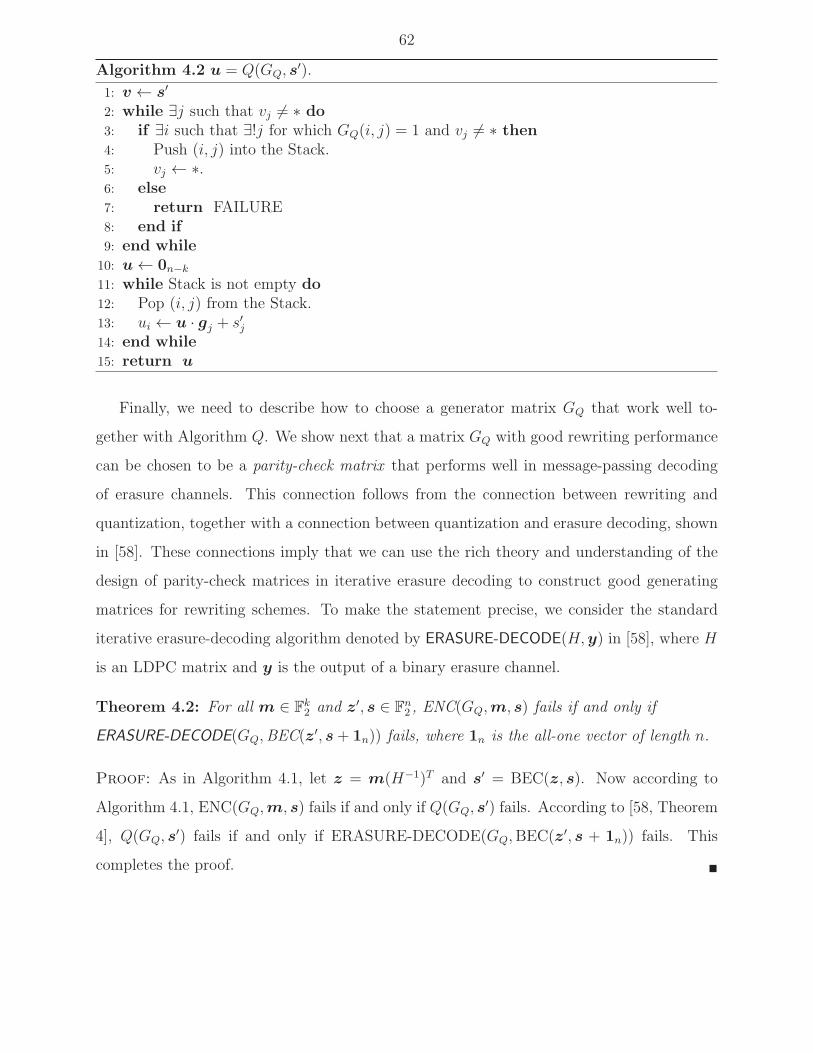
62

Algorithm 4.2 u = Q(GQ, s′).

1: v ← s′

2: while ∃j such that vj 6= ∗ do3: if ∃i such that ∃!j for which GQ(i, j) = 1 and vj 6= ∗ then4: Push (i, j) into the Stack.5: vj ← ∗.6: else

7: return FAILURE8: end if

9: end while

10: u← 0n−k

11: while Stack is not empty do

12: Pop (i, j) from the Stack.13: ui ← u · gj + s′j14: end while

15: return u

Finally, we need to describe how to choose a generator matrix GQ that work well to-

gether with Algorithm Q. We show next that a matrix GQ with good rewriting performance

can be chosen to be a parity-check matrix that performs well in message-passing decoding

of erasure channels. This connection follows from the connection between rewriting and

quantization, together with a connection between quantization and erasure decoding, shown

in [58]. These connections imply that we can use the rich theory and understanding of the

design of parity-check matrices in iterative erasure decoding to construct good generating

matrices for rewriting schemes. To make the statement precise, we consider the standard

iterative erasure-decoding algorithm denoted by ERASURE-DECODE(H,y) in [58], where H

is an LDPC matrix and y is the output of a binary erasure channel.

Theorem 4.2: For all m ∈ Fk2 and z′, s ∈ F

n2 , ENC(GQ,m, s) fails if and only if

ERASURE-DECODE(GQ,BEC(z′, s+ 1n)) fails, where 1n is the all-one vector of length n.

Proof: As in Algorithm 4.1, let z = m(H−1)T and s′ = BEC(z, s). Now according to

Algorithm 4.1, ENC(GQ,m, s) fails if and only if Q(GQ, s′) fails. According to [58, Theorem

4], Q(GQ, s′) fails if and only if ERASURE-DECODE(GQ,BEC(z

′, s + 1n)) fails. This

completes the proof. �

63

The running time of the encoding algorithm ENC is analyzed formally in the following

theorem.

Theorem 4.3: The algorithm ENC(GQ,m, s) runs in time O(nd) where n is the length of

s and d is the maximum degree of the Tanner graph of GQ.

Proof: We first show that Step 1 of Algorithm 4.1 runs in time O(n) if (H−1)T is chosen

in the following way. For any CQ, its parity check matrix H can be made in to systematic

form, i.e., H = (P I), by row operations and permutation of columns. Then (H−1)T can be

chosen as (0k×n−k Ik), and so z = m(H−1)T = (0n−k m).

By [58, Theorem 5], Step 3 of Algorithm 4.1 runs in time O(nd). By the definition of d,

the complexity of Step 7 is also O(nd). Therefore O(nd) dominates the computational cost

of the algorithm. �

Theorems 4.2 and 4.3, together with the analysis and design of irregular LDPC codes

that achieve the capacity of the binary erasure channel [65], imply the following capacity-

achieving results.

Corollary 4.1: There exists a sequence of rewriting codes which can be efficiently encoded

by Algorithm 4.1 and efficiently decoded by Equation (4.1) that achieves the capacity of the

rewriting model β.

Proof: Let s = s+1n. Then it follows from Theorem 4.2 that for all GQ, m ∈ Fk2, z

′ ∈ Fn2 ,

Pr{ENC(GQ,m, s) = Failure} =

Pr{ERASURE-DECODE(GQ,BEC(z′, s)) = Failure},

where s is distributed i.i.d. with Pr{si =} = β. The right-hand side is the decoding-failure

probability of an LDPC code with parity-check matrix GQ over a binary erasure channel,

using message-passing decoding. The erasure probability of the channel is 1 − β, because

Pr{si = 1} = 1 − Pr{si = 1}. The capacity of a binary erasure channel with erasure

64

probability 1 − β is β. This is also the capacity of the rewriting model. In addition, the

rate of an LDPC code with parity-check matrix GQ is equal to the rate of a rewriting code

constructed by the cosets of CQ. It is shown in [65] how to construct a sequence of irregular

LDPC codes that achieves the capacity of the binary erasure channel. Such a sequence, used

for rewriting codes, achieves the rewriting capacity. �

4.2.1 Handling Encoding Failures

The encoding failure event could be dealt with in several ways. A simple solution is to try

writing on different invalid pages, if available, or to simply write onto a fresh page, as current

flash systems do. If the failure rate is small enough, say below 10−3, the time penalty of

rewriting failures would be small. For an alternative solution, we state a reformulation of

[58, Theorem 3].

Proposition 4.1: For all m,m′ ∈ Fk2 and s ∈ F

n2 , ENC(GQ,m, s) fails if and only if

ENC(GQ,m′, s) fails.

Proof: As in Algorithm 4.1, let z = m(H−1)T and s′ = BEC(z, s). Note that

ENC(GQ,m, s) fails if and only if Q(GQ, s′) fails. By Algorithm 4.2, the failure of Q(GQ, s

′)

is determined only according to the locations of erasures in s′, and does not depend on the

values of the non-erased entries of s′. Since s′ = BEC(z, s), the locations of erasures in s′

are only determined by the state s. This completes the proof. �

Proposition 4.1 implies that whether a page is rewritable does not depend on the message

to be written. This property suggests that the flash controller can check whether a page is

rewritable right after it is being invalidated, without waiting for a message to arrive. An

invalid page could be marked as ‘unrewritable’, such that data would be rewritten only into

rewritable pages. This policy would guarantee that the rewriting of a new message always

succeeds. However, this policy also implies that the message passing algorithm would run

more than once for the rewriting of a page.

65

10-5

10-4

10-3

10-2

10-1

100

0.36 0.38 0.4 0.42 0.44 0.46

Rew

ritin

g F

ailu

re R

ate

Code Rate

Polar Code n = 8192Polar Code n = 16384LDGM Code n = 8000

LDGM Code n = 16000

Figure 4.1: Rewriting failure rates of polar and LDGM WOM codes.

4.2.2 Simulation Results

The finite-length performance of our rewriting scheme is evaluated using extensive simulation

with the choice of β = 0.5 and GQ to be the parity-check matrix of a Mackay code [56]. The

rewriting failure rates of our codes with lengths n = 8000 and 16000 that are relevant to flash

applications are compared with those of the polar WOM codes of lengths 213 and 214 [7].

Fig. 4.1 shows the rewriting failure rates of both codes at different rewriting rate, where each

point is calculated from 105 experiments. Remember that the capacity of the model is 0.5.

The results suggest that our scheme achieves a decent rewriting rate (e.g., 0.39) with low

failure rate (e.g., < 10−4). Moreover, our codes provide significantly lower failure rates than

polar WOM codes when the rewriting rate is smaller, because of the good performance in

the waterfall region of message-passing algorithm.

66

4.3 Error-Correcting Rewriting Codes

The construction of error-correcting rewriting codes is based on a pair of linear codes (C1, CQ)

that satisfies the condition C1 ⊇ CQ, meaning that each codeword of CQ is also a codeword of

C1. Define C2 to be the dual of CQ, denoted by C2 = C⊥Q . A pair of linear codes (C1, C2), that

satisfies C1 ⊇ C⊥2 is called a conjugate code pair, and it is useful in quantum error correction

and cryptography [35]. For the flash memory application, we let C1 be an error-correction

code, while C⊥2 = CQ is a BEQ code. The main idea in the construction of error-correcting

rewriting codes is to label only the codewords of C1, according to their membership in the

cosets of CQ. The construction is defined formally as follows:

Construction 4.2: For c ∈ C1, let c+ CQ be the coset of CQ in C1 that contains c. Then

the error-correcting rewriting code is constructed to be the collection of cosets of CQ in C1.

Next we define the matrices (H−1)T and HT to be used in encoding and decoding. Let

G1 and GQ be generator matrices of the codes C1 and CQ, respectively, such that each row

of GQ is also a row of G1. Since C1 contains CQ, such matrix pair always exists. Define

(H−1)T to be constructed by the rows of G1 that are not rows of GQ. Let HT be a right

inverse of (H−1)T .

The encoding is performed according to Algorithm 4.1, with the matrix (H−1)T defined

above. Note that in Step 1, z is a codeword of C1, since each row of (H−1)T is also a row of

G1. In addition, in Step 7, uGQ is also a codeword of C1 (unless Q(GQ, s′) fails), since CQ

is contained in C1. Therefore, x = uGQ + z is a codeword of C1. The decoding can begin

by the recovery of x from its noisy version, using the decoder of C1. The message m can

then be recovered by the product xHT .

A similar framework was described in [41], which proposed a construction of a repetition

code contained in a Hamming code, with a Viterbi encoding algorithm. In this chapter we

make the connection to the quantum coding literature, which allows us to construct stronger

codes.

67

4.3.1 Conjugate Codes Construction

good error-correcting code, while C⊥2 is a good LDGM quantization code. Theorem 4.2

implies that C2 needs to be an LDPC code with a good performance over a binary erasure

channel (under message passing decoding).

Constructions of conjugate code pairs in which C2 is an LDPC code are studied in [34]

[40] [73]. Sarvepalli et al. [73] constructed a pair of codes such that C1 is a BCH code and

C2 is a Euclidean geometry LDPC code, which is particularly useful for our purpose. This

is because BCH codes are used extensively for error correction in flash memories. Below we

first briefly review the construction of Euclidean geometry LDPC codes and then discuss the

application of the results in [73] to our settings.

Denote by EG(m, ps) the Euclidean finite geometry over Fps consisting of pms points.

Note that this geometry is equivalent to the vector space Fmps . A µ-dimensional subspace

of Fmps or its coset is called a µ-flat. Let J be the number of µ-flats that do not contain

the origin, and let α1, ...αpsm−1 be the points of EG(m, ps) excluding the origin. Construct a

J×psm−1 matrixHEG in the way that its (i, j)-th entry equals 1 if the i-th µ-flat contains αj,

and equals 0 otherwise. HEG is the parity check matrix of the (Type-I) Euclidean geometry

LDPC code CEG(m,µ, s, p). CEG(m,µ, s, p) is a cyclic code, and by analyzing the roots of

its generator polynomial the following result is obtained [73]:

Proposition 4.2: C⊥EG(m,µ, s, p) is contained in a BCH code of design distance δ = pµs−1.

Hence we may choose C2 to be CEG(m,µ, s, p) and C1 to be a BCH code with distance

equal to or smaller than δ. Some possible code constructions are shown in Table 4.1. Their

encoding performance, with respect to the probability β that a cell in the state is writable, is

shown in Fig. 4.2. Note from Fig. 4.2 that a code with smaller rewriting rate achieves a fixed

failure rate at a smaller value of β. In particular, the codes corresponding to the top three

rows of Table 4.1 achieve very small failure rate at β = 0.5, the point of practical interest.

These results also show that the slope of the figures becomes sharper when the length of the

codes increases, as expected. Out of the three codes that can be rewritten with β = 0.5,

68

Table 4.1: Error-correcting Rewriting Codes Constructed from Pairs of Conjugate BCH andEG-LDPC Codes.

(m,µ, s, p) C1[n, k, δ] C2[n, k] Rewriting Rate(4,1,2,2) [255,247,3] [255,21] 0.0510(3,1,2,2) [65,57,3] [65,13] 0.1111(3,1,3,2) [511,484,7] [511,139] 0.2192(3,1,4,2) [4095,4011,15] [4095,1377] 0.3158

CEG(3, 1, 3, 2) poses the best rate and error-correction capability.

0

0.2

0.4

0.6

0.8

1

0 0.1 0.2 0.3 0.4 0.5 0.6

Rew

ritin

g F

ailu

re R

ate

β

(3, 1, 2, 2)(4, 1, 2, 2)

(3, 1, 3, 2)(3, 1, 4, 2)

Figure 4.2: Encoding performance of the codes in Table 4.1.

In this section we present two alternative approaches to combine rewriting codes with

error correction.

4.3.2 Concatenated Codes

In this scheme, we concatenate an LDGM rewriting code with a systematic error-correcting

code. The outer code is an LDGM rewriting code without error-correction capability, as in

Section 4.2. The systematic ECC is used as the inner code. The concatenated scheme is

69

used in the second write. The scheme requires the first write to reserve some bits to store

the redundancy of the ECC in the second write.

In the second write, the encoder begins by finding a vector x that can be written over

the current state. After x is written, the systematic ECC calculates the redundancy bits

required to protect x from errors. The redundancy bits are then written into the reserved

cells. The decoding of the second write begins by recovering x using the systematic ECC

and its redundancy bits. After x is recovered, the decoder of the rewriting code recovers the

stored message from x.

We note that reserving bits for the second write have a negative effect on the performance

of the system, since it reduces the total amount of information that can be stored in the

memory on a given time. Therefore, the next subsection extends the concatenation scheme

using a chaining technique, with the aim of reducing the number of bits required to be

reserved for the second write.

4.3.3 Code Chaining

The chaining approach is inspired by a similar construction in polar coding [63]. The idea

is to chain several code blocks of short length. In the following we use a specific example to

demonstrate the idea. We use a BCH code for error correction, since its performance can be

easily calculated. We note, however, that LDPC codes may be used in practice, such that

the circuit modules may be shared with the rewriting code, to reduce the required area. The

performance of LDPC code in the considered parameters is similar to that of BCH codes.

A typical BCH code used in flash memory has the parameters [8191, 7671, 81], where the

length is 8191, the dimension is 7671, and the minimum distance is 81. If this code is used in

a concatenated scheme for the second write, the first write needs to reserve 8191−7671 = 520

bits for redundancy.

To reduce the amount of required reserved bits, we consider the chaining of 8 systematic

BCH codes with the parameters [1023, 863, 33]. The encoding is performed sequentially,

beginning with the rewriting encoding that finds a vector x1 of 863 bits. The vector x1

70

represents a message m1 of 310 bits, according to an [863, 310]-LDGM rewriting code. Once

x1 is found, the BCH encoder finds 1023−863 = 160 redundancy bits to protect x1, as in the

concatenated scheme. The encoder then “chains” the redundancy bits forward, by encoding

them, together with 150 new information bits, into another block of 863 bits, using the

[863, 310]-LDGM code. Let m2 denote the vector of 310 bits encoded into the second block.

m2 contains the 160 redundancy bits of x1, together with the additional 150 information

bits. Note that once m2 is decoded, the redundancy bits of x1 are available, allowing the

recovery x1, and then m1. The encoding continues in this fashion 8 times, to write over a

total of 8 blocks, each containing 863 cells. The 160 redundant bits used to protect x8 are

stored in the reserved cells. The decoding is done in the reverse order, where each decoded

vector contains the redundancy bits of the previous block.

4.3.4 Comparison

We compare the different error-correction approaches, and discuss their trade-offs. The

first code in the comparison is a conjugate code pair, described in Section 4.3. We use

a conjugation of a [511, 484, 7]-BCH code containing a [511, 372]-LDGM code, dual to the

(3, 1, 3, 2)-Euclidean geometry LDPC code in Table 4.1. The second code in the comparison

is a concatenation of an outer [7671, 2915]-LDGM Mackay rewriting code with an inner

[8191, 7671, 81]-BCH code. The third code is a chaining of 8 blocks of [863, 310]-LDGM

Mackay codes, each concatenated with a [1023, 863, 33]-BCH code. We compare the decoding

BER PD, the fraction α of bits required to be reserved, and the rewriting rate RWOM of the

codes. The encoding failure rate of each of the three codes for β = 0.5 is below 10−3. PD is

estimated with a standard flash memory assumption of a raw BER of 1.3×10−3. To achieve

a comparable code length, the conjugated code is assumed to be used 16 times in parallel,

with a total length of 511× 16 = 8176. The comparison is summarized in Table 4.2.

Flash systems require PD below 10−15. We see in Table 4.2 that conjugated code still do

not satisfy the reliability requirement. We also see that concatenated codes that satisfy the

reliability requirement need a large fraction of reserved space. The chained code reduces the

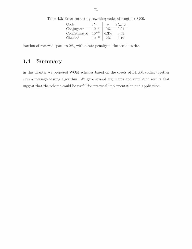
71

Table 4.2: Error-correcting rewriting codes of length ≈ 8200.

Code PD α RWOM

Conjugated 10−5 0% 0.21Concatenated 10−16 6.3% 0.35Chained 10−16 2% 0.19

fraction of reserved space to 2%, with a rate penalty in the second write.

4.4 Summary

In this chapter we proposed WOM schemes based on the cosets of LDGM codes, together

with a message-passing algorithm. We gave several arguments and simulation results that

suggest that the scheme could be useful for practical implementation and application.

72

Chapter 5

Rewriting with Polar Codes

The material in this chapter was presented in part in [21]. In this chapter we present a new

construction of polar WOM codes. We first discuss the relation of the result to previous

work.

5.1 Relation to Previous Work

The study of channel coding with an informed encoder was initiated by Kusnetsov and Tsy-

bakov [51], with the channel capacity derived by Gelfand and Pinsker [28]. The informed

encoding technique of Gelfand and Pinsker was used earlier by Marton to establish an inner

bound for the capacity region of broadcast channels [59]. Low-complexity capacity-achieving

codes were first proposed for continuous channels, using lattice codes [90]. In discrete chan-

nels, the first low-complexity capacity-achieving scheme was proposed using polar codes, for

the symmetric special case of information embedding [50, Section VIII.B]. A modification

of this scheme for the WOM model was proposed in [7]. An additional capacity-achieving

WOM scheme, based on randomness extractors, was also proposed recently [25].

Our work is concerned with a setup that is similar to those considered in [7, 25]. An

important contribution of the current work compared to [7, 25] is that our scheme achieves

the capacity of a rewriting model that also includes noise, while the schemes in [7,25] address

only the noiseless case. Indeed, error correction is a crucial capability in flash memory

73

systems. Our low-complexity achievability of the noisy capacity is done using a multicoding

technique. Compared with [25], the current work allows an input cost constraint, which

is important in rewriting models for maximizing the sum of the code rates over multiple

rewriting rounds. Compared with [7], the current work also improves by removing the

requirement for shared randomness between the encoder and the decoder, which limits the

practical coding performance. The removal of the shared randomness is done by the use of

non-linear polar codes. An additional coding scheme was proposed during the writing of this

thesis, and which also does not require shared randomness [55]. However, the scheme in [55]

considers only the noiseless case, and it is in fact a special case of the scheme in the current

chapter.

Polar coding for channels with informed encoders was implicitly studied recently in the

context of broadcast channels, as the Marton coding scheme for broadcast communication

contains an informed encoding instance as an ingredient. In fact, a multicoding technique

similar to the one presented in this chapter was recently presented for broadcast channels,

in [29]. While we were unaware of the result of [29] and developed the scheme indepen-

dently, this chapter also has three contributions that were not shown in [29]. First, by

using the modified scheme of non-linear polar codes, we reduce the storage requirement

from an exponential function in the block length to a linear function. Secondly, we connect

the scheme to the application of data storage and flash memory rewriting, which was not

considered in the previous work. And thirdly, the analysis in [29] holds only for channels

whose capacity-achieving distribution forms a certain degraded structure. In this chapter we

consider a specific noisy rewriting model, whose capacity-achieving distribution forms the

required degraded structure, and by that we show that the scheme achieves the capacity of

the considered flash-memory model.

Another recent paper on polar coding for broadcast channels was published recently by

Mondelli et. al. [63]. That paper used the chaining method (as in Subsection 4.3.3), which

allows one to bypass the degraded structure requirement. In this chapter we connect the

chaining method to the flash-memory rewriting application and to our new non-linear polar

74

coding scheme, and apply it to our proposed multicoding scheme. This allows for a linear

storage requirement, together with the achievability of the informed encoder capacity and

Marton’s inner bound, eliminating the degraded structure requirement. Finally, we show an

important instance of the chaining scheme for a specific flash-memory model, and explain

the applicability of this instance in flash-memory systems.

A special case of the proposedWOM construction is that of point-to-point channel coding.

The proposed construction also contributes to the literature on point-to-point channel cod-

ing, in the case that the channel is asymmetric. Several polar coding schemes for asymmetric

channels were proposed recently, including a pre-mapping using Gallager’s scheme [26, p.

208] and a concatenation of two polar codes [80]. A more direct approach was proposed

in [37], and also considered in [62]. The scheme in [37] achieves the capacity of asymmet-

ric channels using non-linear polar codes, but it uses large Boolean functions that require

storage space that is exponential in the block length. We propose a modification for this

scheme that removes the requirement for the Boolean functions, and thus reduces the storage

requirement of the encoding and decoding tasks to a linear function of the block length.

We start by describing the special case of asymmetric channels in Section 5.2. We then

move to the WOM case in Section 5.3, which proposes a polar multicoding scheme for

channels with informed encoders, including two special cases of noisy WOM.

5.2 Asymmetric Point-to-Point Channels

Notation: For positive integers m ≤ n, let [m : n] denote the set {m,m+ 1, . . . , n}, and let

[n] denote the set [1 : n]. Given a subset A of [n], let Ac denote the complement of A with

respect to [n], where n is clear from the context. Let x[n] denote a vector of length n, and

let xA denote a vector of length |A| obtained from x[n] by deleting the elements with indices

in Ac.

Throughout this section we consider only channels with binary input alphabets, since the

literature on polar codes with non-binary codeword symbols is relatively immature. However,

75

the results of this section can be extended to non-binary alphabets without much difficulty

using the methods described in [64, 66, 72, 74–76]. The main idea of polar coding is to take

advantage of the polarization effect of the Hadamard transform on the entropies of random

vectors. Consider a binary-input memoryless channel model with an input random variable

(RV) X ∈ {0, 1}, an output RV Y ∈ Y and a pair of conditional probability mass functions

(pmfs) pY |X(y|0), pY |X(y|1) on Y . Let n be a power of 2 that denotes the number of channel

uses, also referred to as the block length. The channel capacity is the tightest upper bound

on the code rate in which the probability of decoding error can be made as small as desirable

for a large enough block length. The channel capacity is given by the mutual information of

X and Y .

Theorem 5.1: (Channel Coding Theorem) [13, Chapter 7] The capacity of the discrete

memoryless channel p(y|x) is given by

C = maxp(x)

I(X;Y ).

The Hadamard transform is a multiplication of the random vector X[n] over the field

of cardinality 2 with the matrix Gn = G⊗ log2 n, where G =

1 0

1 1

and ⊗ denotes the

Kronecker power. In other words, Gn can be described recursively for n ≥ 4 by the block

matrix

Gn =

Gn/2 0

Gn/2 Gn/2

.

The matrix Gn transforms X[n] into a random vector U[n] = X[n]Gn, such that the con-

ditional entropy H(Ui|U[i−1], Y[n]) is polarized. That means that for a fraction of close to

H(X|Y ) of the indices i ∈ [n], the conditional entropy H(Ui|U[i−1], Y[n]) is close to 1, and for

almost all the rest of the indices, H(Ui|U[i−1], Y[n]) is close to 0. This result was shown by

Arikan in [1, 2].

Theorem 5.2: (Polarization Theorem) [2, Theorem 1] Let n, U[n], X[n], Y[n] be defined

76

as above. For any δ ∈ (0, 1), let

HX|Y ,{

i ∈ [n] : H(Ui|U[i−1], Y[n]) ∈ (1− δ, 1)}

,

and

LX|Y ,{

i ∈ [n] : H(Ui|U[i−1], Y[n]) ∈ (0, δ)}

.

Then

limn→∞

|HX|Y |/n = H(X|Y ) and limn→∞

|LX|Y |/n = 1−H(X|Y ).

Note thatH(X|Y ) denotes a conditional entropy, whileHX|Y denotes a subset of [n]. It is also

shown in [1] that the transformation Gn is invertible with G−1n = Gn, implying X[n] = U[n]Gn.

This polarization effect can be used quite simply for the design of a coding scheme that

achieves the capacity of symmetric channels with a running time that is polynomial in the

block length. The capacity of symmetric channels is achieved by a uniform distribution on

the input alphabet, i.e., p(x) = 1/2 [13, Theorem 7.2.1]. Since the input alphabet in this

chapter is binary, the capacity-achieving distribution gives H(X) = 1, and therefore we have

limn→∞

(1/n)|LX|Y | = 1−H(X|Y ) = H(X)−H(X|Y ) = I(X;Y ) = C. (5.1)

Furthermore, for each index in LX|Y , the conditional probability p(ui|u[i−1], y[n]) must be

close to either 0 or 1 (since the conditional entropy is small by the definition of the set

LX|Y ). It follows that the RV Ui can be estimated reliably given u[i−1] and y[n]. This fact

motivates the capacity-achieving coding scheme that follows. The encoder creates a vector

u[n] by assigning the subvector ULX|Ywith the source message, and the subvector ULc

X|Ywith

uniformly distributed random bits that are shared with the decoder. The randomness sharing

is useful for the analysis, but is in fact unnecessary for using the scheme (the proof of this fact

is described in [1, Section VI]). The set ULcX|Y

is called the frozen set. Equation (5.1) implies

that this coding rate approaches the channel capacity. The decoding is performed iteratively,

from index 1 up to n. In each iteration, the decoder estimates the bit ui using the shared

77

information or using a maximum likelihood estimation, according to the set membership of

the iteration. The estimations of the bits ui for which i is in LcX|Y are always successful,

since these bits were known to the decoder in advance. The rest of the bits are estimated

correctly with high probability, leading to a successful decoding of the entire message with

high probability.

However, this reasoning does not translate directly to asymmetric channels. Remember

that the capacity-achieving input distribution of asymmetric channels is in general not uni-

form (see, for example, [32]), i.e., pX(1) 6= 1/2. Since the Hadamard transform is bijective,

it follows that the capacity-achieving distribution of the polarized vector U[n] is non uniform

as well. The problem with this fact is that assigning uniform bits of message or shared ran-

domness changes the distribution of U[n], and consequentially also changes the conditional

entropies H(Ui|U[i−1], Y[n]). To manage this situation, our approach is to make sure that the

change in the distribution of U[n] is kept to be minor, and thus its effect on the probability of

decoding error is also minor. To do this, we consider the conditional entropies H(Ui|U[i−1]),

for i ∈ [n]. Since the polarization happens regardless of the channel model, we can consider

a channel for which the output Y is a deterministic variable, and conclude by Theorem 5.2

that the entropies H(Ui|U[i−1]) also polarize. For this polarization, a fraction of H(X) of

the indices admit a high H(Ui|U[i−1]). To ensure a minor change in the distribution of U[n],

we restrict the assignments of uniform bits of message and shared randomness to the indices

with high H(Ui|U[i−1]).

The insight of the last paragraph motivates a modified coding scheme. The locations

!"#$%&'()*+'

,%++-.%'()*+'

pUi |U[ i−1]

(u | u[i−1])

LcX|Y !

LX|Y !

HX !HcX !

Figure 5.1: Encoding the vector u[n].

78

with high entropy H(Ui|U[i−1]) are assigned with uniformly distributed bits, while the rest of

the locations are assigned with the pmf p(ui|u[i−1]). Note that p(u[n], x[n]) and H(U[n]) refer

to the capacity-achieving distribution of the channel, which does not equal the distribution

that the encoding process induces. Similar to the notation of Theorem 5.2, we denote the

set of indices with high entropy H(Ui|U[i−1]) by HX . To achieve a reliable decoding, we

place the message bits in the indices of HX that can be decoded reliably, meaning that

their entropies H(Ui|U[i−1], Y[n]) are low. So we say that we place the message bits in the

intersection HX ∩LX|Y . The locations whose indices are not in LX|Y must be known by the

decoder in advance for a reliable decoding. Previous work suggested sharing random Boolean

functions between the encoder and the decoder, drawn according to the pmf p(ui|u[i−1]), and

to assign the indices in (HX ∩ LX|Y )c = Hc

X ∪ LcX|Y according to these functions [29, 37].

However, we note that the storage required for those Boolean functions is exponential in n,

and therefore we propose an efficient alternative.

To avoid the Boolean function, we divide the complement of HX∩LX|Y into three disjoint

sets. First, the indices in the intersection HX ∩LcX|Y are assigned with uniformly distributed

random bits that are shared between the encoder and the decoder. As in the symmetric case,

this randomness sharing will in fact not be necessary, and a deterministic frozen vector could

be shared instead. The rest of the bits of U[n] (those in the set HcX) are assigned randomly

to a value u with probability pUi|U[i−1](u|u[i−1]) (where pUi|U[i−1]

is calculated according to

the pmf pU[n],X[n],Y[n], the capacity-achieving distribution of the channel). The indices in

HcX ∩ LX|Y could be decoded reliably, but not those in Hc

X ∩ LcX|Y . Fortunately, the set

HcX ∩ Lc

X|Y can be shown to be small (as we will show later), and thus we could transmit

those locations separately with a vanishing effect on the code rate. The encoding of the

vector u[n] is illustrated in Figure 5.1.

The see the intuition of why the code rate approaches the channel capacity, notice that

the source message is placed in the indices in the intersection HX ∩ LX|Y . The asymptotic

79

fraction of this intersection can be derived as following:

|HX ∩ LX|Y |/n = 1− |HcX ∪ Lc

X|Y |/n = 1− |HcX |/n− |Lc

X|Y |/n+ |HcX ∩ Lc

X|Y |/n. (5.2)

The Polarization Theorem (Theorem 5.2) implies that |HcX |/n→ 1−H(X) and |Lc

X|Y |/n→H(X|Y ). Since the fraction |Hc

X ∩ LcX|Y | vanishes for large n, we get that the asymptotic

rate is |HX ∩ LX|Y |/n→ H(X)−H(X|Y ) = I(X;Y ), achieving the channel capacity.

For a more precise definition of the scheme, we use the so called Bhattacharyya parameter

in the selection of subsets of U[n], instead of the conditional entropy. The Bhattacharyya

parameters are polarized in a similar manner as the entropies, and are more useful for

bounding the probability of decoding error. For a discrete RV Y and a Bernoulli RV X, the

Bhattacharyya parameter is defined by

Z(X|Y ) , 2∑

y

√

pX,Y (0, y)pX,Y (1, y). (5.3)

Note that most of the polar coding literature uses a slightly different definition of the Bhat-

tacharyya parameter that coincides with Equation (5.3) when the RV X is distributed

uniformly. We use the following relations between the Bhattacharyya parameter and the

conditional entropy.

Proposition 5.1: ( [2, Proposition 2])

(Z(X|Y ))2 ≤ H(X|Y ), (5.4)

H(X|Y ) ≤ log2(1 + Z(X|Y )) ≤ Z(X|Y ). (5.5)

We now define the set of high and low Bhattacharyya parameters, and work with them

80

instead of the sets HX|Y and LX|Y . For δ ∈ (0, 1), define

HX|Y ,

{

i ∈ [n] : Z(Ui|U[i−1], Y[n]) ≥ 1− 2−n1/2−δ}

,

LX|Y ,

{

i ∈ [n] : Z(Ui|U[i−1], Y[n]) ≤ 2−n1/2−δ}

.

As before, we define the sets HX and LX for the parameter Z(Ui|U[i−1]) by letting Y[n] be

a deterministic vector. Using Proposition 5.1, it is shown in [37, combining Proposition 2

with Theorem 2] that Theorem 5.2 holds also if we replace the sets HX|Y and LX|Y with the

sets HX|Y and LX|Y . That is, we have

limn→∞

|HX|Y |/n = H(X|Y ) and limn→∞

|LX|Y |/n = 1−H(X|Y ). (5.6)

We now define our coding scheme formally. Let m[|HX∩LX|Y |] ∈ {0, 1}|HX∩LX|Y | be the

realization of a uniformly distributed source message, and f[|HX∩LcX|Y

|] ∈ {0, 1}|HX∩LcX|Y

| be

a deterministic frozen vector known to both the encoder and the decoder. We discuss how

to find a good frozen vector in Appendix 5.6.3. For a subset A ⊆ [n] and an index i ∈ A, weuse a function r(i,A) to denote the rank of i in an ordered list of the elements of A. The

probabilities pUi|U[i−1](u|u[i−1]) and pUi|U[i−1],Y

n(u|u[i−1], y[n]) can be calculated efficiently by a

recursive method described in [37, Section III.B].

Construction 5.1:

Encoding

Input: a message m[|HX∩LX|Y |] ∈ {0, 1}|HX∩LX|Y |.

Output: a codeword x[n] ∈ {0, 1}n.

1. For i from 1 to n, successively, set

ui =

u ∈ {0, 1} with probability pUi|U[i−1](u|u[i−1]) if i ∈ Hc

X

mr(i,HX∩LX|Y ) if i ∈ HX ∩ LX|Y

fr(i,HX∩LcX|Y

) if i ∈ HX ∩ LcX|Y .

81

2. Transmit the codeword x[n] = u[n]Gn.

3. Transmit the vector uHcX∩Lc

X|Yseparately using a linear, non-capacity-achieving polar

code with a uniform input distribution (as in [1]). In practice, other error-correcting

codes could be used for this vector as well.

Decoding

Input: a noisy vector y[n] ∈ {0, 1}n.Output: a message estimation m[|HX∩LX|Y |] ∈ {0, 1}|HX∩LX|Y |.

1. Estimate the vector uHcX∩Lc

X|Yby uHc

X∩LcX|Y

.

2. For i from 1 to n, set

ui =

argmaxu∈{0,1}

pUi|U[i−1],Y[n](u|u[i−1], y[n]) if i ∈ LX|Y

ur(i,HcX∩Lc

X|Y) if i ∈ Hc

X ∩ LcX|Y

fr(i,HX∩LcX|Y

) if i ∈ HX ∩ LcX|Y .

3. Return the estimated message m[|HX∩LX|Y |] = uHX∩LX|Y.

We say that a sequence of coding schemes achieves the channel capacity if the probability

of decoding error vanishes with the block length for any rate below the capacity.

Theorem 5.3: Construction 5.1 achieves the channel capacity (Theorem 5.1) with a com-

putational complexity of O(n log n) and a probability of decoding error of 2−n1/2−δfor any

δ > 0 and large enough n.

In the next section we show a generalized construction and prove its capacity-achieving

property. Theorem 5.3 thus will follow as a corollary of the more general Theorem 5.7.

82

5.3 Channels with Non-Causal Encoder State Informa-

tion

In this section we generalize Construction 5.1 to the availability of channel state information

at the encoder. We consider mainly the application of rewriting in flash memories (WOM),

and present two special cases of the channel model for this application. We model the memory

cells as a channel with a discrete state, and we also assume that the state is memoryless,

meaning that the states of different cells are distributed independently. We assume that

the state of the entire n cells is available to the writer prior to the beginning of the writing

process. In communication terminology this kind of state availability is refereed to as “non

causal”. We note that this setting is also useful in the so called Marton-coding method for

communication over broadcast channels. Therefore, the multicoding schemes that will follow

serve as an additional contribution in this important setting.

We represent the channel state as a Bernoulli random variable S with parameter β, which

equals the probability p(S = 1). A cell of state 1 can only be written with the value 1. Note

that, intuitively, when β is high, the capacity of the memory is small, since only a few

cells are available for modification in the writing process, and thus only a small amount of

information could be stored. This also means that the choice of codebook has a crucial effect

on the capacity of the memory in future writes. A codebook that contains many codewords

of high Hamming weight (number of 1’s in the codeword) would make the parameter β

of future writes high, and thus the capacity of the future writes would be low. However,

forcing the expected Hamming weight of the codebook to be low would reduce the capacity

of the current write. To settle this trade-off, previous work suggested to optimize the sum

of the code rates over multiple writes. It was shown that in many cases, constraints on the

codebook Hamming weight (henceforth just weight) strictly increase the sum rate (see, for

example, [36]). Therefore, we consider an input cost constraint in the model.

The most general model that we consider is a discrete memoryless channel (DMC) with

a discrete memoryless (DM) state and an input cost constraint, where the state information

83

is available non-causally at the encoder. The channel input, state, and output are denoted

by x, s, and y, respectively, and their respective finite alphabets are denoted by X ,S, andY . The random variables are denoted by X,S, and Y , and the random vectors by X[n], S[n],

and Y[n], where n is the block length. The state is distributed according to the pmf p(s),

and the conditional pmfs of the channel are denoted by p(y|x, s). The input cost function is

denoted by b(x), and the input cost constraint is

n∑

i=1

E[b(Xi)] ≤ nB,

where B is a real number representing the normalized constraint. The channel capacity with

an informed encoder and an input cost constraint is given by an extension of the Gelfand-

Pinsker Theorem1.

Theorem 5.4: (Gelfand-Pinsker Theorem with Cost Constraint) [16, Equation

(7.7) on p. 186] The capacity of a DMC with a DM state p(y|x, s)p(s) and an input cost

constraint B when the state information is available non causally only at the encoder is

C = maxp(v|s),x(v,s):E(b(X))≤B

(I(V ;Y )− I(V ;S)), (5.7)

where V is an auxiliary random variable with a finite alphabet V,|V| ≤ min {|X · S,Y + S − 1}.

The main coding scheme that we present in this section achieves the capacity in Theo-

rem 5.4. The proof of Theorem 5.4 considers a virtual channel model, in which the RV V is

the channel input and Y is the channel output. Similar to the previous section, we limit the

treatment to the case in which the RV V is binary. In flash memory, this case would corre-

spond to a single-level cell (SLC) type of memory. As mentioned in Section 5.2, an extension

of the scheme to a non-binary case is not difficult. The non-binary case is useful for flash

1The cost constraint is defined slightly differently in this reference, but the capacity is not affected bythis change.

84

memories in which each cell stores 2 or more bits of information. Such memories are called

Multi-Level Cell (MLC). We also mention that the limitation to binary random variables

does not apply on the channel output Y . Therefore, the cell voltage in flash memory could

be read more accurately at the decoder to increase the coding performance, similarly to the

soft decoding method that is used in flash memories with LDPC codes. Another practical

remark is that the binary-input model can be used in MLC memories by coding separately

on the MSB and the LSB of the cells, as is in fact the coding method in current MLC flash

systems.

The scheme that achieves the capacity of Theorem 5.4 is called Construction 5.3, and it

will be described in Subsection 5.3.3. The capacity achieving result is summarized in the

following theorem, which will be proven in Subsection 5.3.3.

Theorem 5.5: Construction 5.3 achieves the capacity of the Gelfand-Pinsker Theorem with

Cost Constraint (Theorem 5.4) with a computational complexity of O(n log n) and a proba-

bility of decoding error of 2−n1/2−δfor any δ > 0 and large enough n.

Note that the setting of Theorem 5.5 is a generalization of the asymmetric channel-

coding setting of Theorem 5.3, and therefore Construction 5.3 and Theorem 5.5 are in

fact a generalization of Construction 5.1 and Theorem 5.3. Before we describe the code

construction, we first show in Subsection 5.3.1 two special cases of the Gelfand-Pinsker

model that are useful for the rewriting of flash memories. Afterwards, in subsections 5.3.2

and 5.3.3, we will show two versions of the construction that correspond to generalizations

of the two special cases.

5.3.1 Special Cases

We start with a special case that is quite a natural model for flash memory rewriting.

Example 5.1: Let the sets X ,S, and Y be all equal to {0, 1}, and let the state pmf be

pS(1) = β. This model corresponds to a single level cell flash memory. We describe the

cell behaviour after a bit x is attempted to be written. When s = 0, the cell behaves as

85

1 1

0 0

1 1

0 0

S = 0 S = 1

α1 α1

α0 1− α1

1− α1 1− α1

α11− α0

X YX Y

Figure 5.2: Example 5.1: A binary noisy WOM model.

a binary asymmetric channel with input x, since the call state does not interfere with the

writing attempt. When s = 1, the cell behaves as if a value of 1 was attempted to be written,

regardless of the actual value x attempted. However, an error might still occur, during the

writing process or anytime afterwards (for example, due to charge leakage). Thus, we can

say that when s = 1, the cell behaves as a binary asymmetric channel with input 1. Formally,

the channel pmfs are given by

pY |XS(1|x, s) =

α0 if (x, s) = (0, 0)

1− α1 if (x, s) = (0, 1)

1− α1 if (x, s) = (1, 0)

1− α1 if (x, s) = (1, 1)

(5.8)

The error model is also presented in Figure 5.2. The cost constraint is given by b(xi) = xi,

since it is desirable to limit the amount of cells written to a value of 1.

Our coding-scheme construction for the setting of Theorem 5.4 is based on a more limited

construction, which serves as a building block. We will start by describing the limited

construction, and then show how to extend it for the model of Theorem 5.4. We will prove

that the limited construction achieves the capacity of channels whose capacity-achieving

distribution forms a certain stochastically degraded structure. We first recall the definition

of stochastically degraded channels.

Definition 5.1: [16, p. 112] A discrete memoryless channel (DMC) W1 : {0, 1} → Y1

is stochastically degraded (or simply degraded) with respect to a DMC W2 : {0, 1} → Y2,

86

0 0

1− α

1− α

α

α

X X YY

S = 0 S = 1

1 1

0

11

Figure 5.3: Example 5.2: A binary WOM with writing noise.

denoted as W1 � W2, if there exists a DMC W : Y2 → Y1 such that W satisfies the equation

W1(y1|x) =∑

y2∈Y2W2(y2|x)W (y1|y2).

Next, we bring the required property of channels whose capacity is achieved by the limited

construction to be proposed.

Property 5.1: There exist functions p(v|s) and x(v, s) that maximize the Gelfand-Pinsker

capacity in Theorem 5.4 and satisfy the condition p(y|v) � p(s|v).

It is an open problem whether or not the model of Example 5.1 satisfies the degradation

condition of Property 5.1. However, we can modify the model such that it will satisfy

Property 5.1. Specifically, we study the following model:

Example 5.2: Let the sets X ,S and Y be all equal to {0, 1}. The channel and state pmfs

are given by pS(1) = β and

pY |XS(1|x, s) =

α if (x, s) = (0, 0)

1− α if (x, s) = (1, 0)

1 if s = 1.

(5.9)

In words, if s = 1 the channel output is always 1, and if s = 0, the channel behave as a

binary symmetric channel. The cost function is given by b(xi) = xi. The error model is also

presented in Figure 5.3. This model can represent a writing noise, as a cell of state s = 1 is

not written on and it never suffers errors.

87

We claim that the model of Example 5.2 satisfies the degradation condition of Prop-

erty 5.1. To show this, we need first to find the functions p(v|s) and x(v, s) that maximize

the Gelfand-Pinsker capacity in Theorem 5.4. Those functions are established in the follow-

ing theorem.

Theorem 5.6: The capacity of the channel in Example 5.2 is

C = (1− β)[h(ǫ ∗ α)− h(α)],

where ǫ = B/(1−β) and ǫ∗α ≡ ǫ(1−α)+(1−ǫ)α. The selections V = {0, 1}, x(v, s) = v∧¬s(where ∧ is the logical AND operation, and ¬ is the logical negation), and

pV |S(1|0) = ǫ, pV |S(1|1) =ǫ(1− α)

ǫ ∗ α (5.10)

achieve this capacity.

Theorem 5.6 is similar to [36, Theorem 4], and its proof is described in Section 5.5.

Intuitively, the upper bound is obtained by assuming that the state information is available

also at the decoder, and the lower bound is obtained by setting the functions x(v, s) and

p(v|s) according to the statement of the theorem. The proof that the model in Example 5.2

satisfies the degradation condition of Property 5.1 is completed by the following lemma.

Lemma 5.1: The capacity achieving functions of Theorem 5.6 for the model of Example 5.2

satisfy the degradation condition of Property 5.1. That is, the channel p(s|v) is degraded with

respect to the channel p(y|v).

Lemma 5.1 is proven in Section 5.5, and consequently the capacity of the model in Exam-

ple 5.2 can be achieved by our limited construction. In the next subsection we describe the

construction for channel models that satisfy Property 5.1, including the model in Exam-

ple 5.2.

88

5.3.2 Multicoding Construction for Degraded Channels

Notice first that the capacity-achieving distribution of the asymmetric channel in Section 5.2

actually satisfies Property 5.1. In the asymmetric channel-coding case, the state can be

thought of as a degenerate random variable (a RV which only takes a single value), and

therefore we can choose W in Definition 5.1 to be degenerate as well, and by that satisfy

Property 5.1. We will see that the construction that we present in this subsection is a

generalization of Construction 5.1.

The construction has a similar structure as the achievability proof of the Gelfand-Pinsker

Theorem (Theorem 5.4). The encoder first finds a vector v[n] in a similar manner to Con-

struction 5.1, where the RV X|Y in Construction 5.1 is replaced with V |Y , and the RV X

is replaced with V |S. The vector U[n] is now the polarization of the vector V[n], meaning

that U[n] = V[n]Gn. The RV V is taken according to the pmfs p(v|s) that maximize the rate

expression in Equation (5.7). The selection of the vector u[n] is illustrated in Figure 5.4.

After the vector u[n] is chosen, each bit i ∈ [n] in the codeword x[n] is calculated by the

function xi(vi, si) that maximizes Equation (5.7). To use the model of Example 5.2, one

should use the functions p(v|s) and x(v, s) according to Theorem 5.6. The key to showing

that the scheme achieves the channel capacity is that the fraction |HcV |S ∩ Lc

V |Y |/n can be

shown to vanish for large n if the channel satisfies Property 5.1. Then, by the same intuition

as in Equation (5.2) and using Equation (5.6), the replacements imply that the asymptotic

rate of the codes is

!"#$%&'()*+'

,%++-.%'()*+'

pUi |U[ i−1],S[n ](u | u

[i−1], s[n])

LcV|Y !

LV|Y!

HV|S !Hc

V|S !

Figure 5.4: Encoding the vector u[n] in Construction 5.2.

89

|HV |S ∩ LV |Y |/n = 1− |HcV |S|/n− |Lc

V |Y |/n+ |HcV |S ∩ Lc

V |Y |/n

→ 1− (1−H(V |S))−H(V |Y ) + 0

= I(V ;Y )− I(V ;S),

achieving the Gelfand-Pinsker capacity of Theorem 5.4. We now describe the coding scheme

formally.

Construction 5.2:

Encoding

Input: a message m[|HV |S∩LV |Y |] ∈ {0, 1}|HV |S∩LV |Y | and a state s[n] ∈ {0, 1}n.Output: a codeword x[n] ∈ {0, 1}n.

1. For each i from 1 to n, assign

ui =

u ∈ {0, 1} with probability pUi|U[i−1],S[n](u|u[i−1], s[n]) if i ∈ Hc

V |S

mr(i,HV |S∩LV |Y ) if i ∈ HV |S ∩ LV |Y

fr(i,HV |S∩LcV |Y

) if i ∈ HV |S ∩ LcV |Y .

(5.11)

2. Calculate v[n] = u[n]Gn and for each i ∈ [n], store the value xi(vi, si).

3. Store the vector uHcV |S

∩LcV |Y

separately using a point-to-point linear non-capacity-achieving

polar code with a uniform input distribution. The encoder here does not use the state

information in the encoding process, but rather treats it as an unknown part of the

channel noise.

Decoding

Input: a noisy vector y[n] ∈ {0, 1}n.Output: a message estimation m[|HV |S∩LV |Y |] ∈ {0, 1}|HV |S∩LV |Y |.

1. Estimate the vector uHcV |S

∩LcV |Y

by uHcV |S

∩LcV |Y

.

90

2. Estimate u[n] by u[n](y[n], f[|HV |S∩LcV |Y

|]) as follows: For each i from 1 to n, assign

ui =

argmaxu∈{0,1}

pUi|U[i−1],Y[n](u|u[i−1], y[n]) if i ∈ LV |Y

ur(i,HcV |S

∩LcV |Y

) if i ∈ HcV |S ∩ Lc

V |Y

fr(i,HV |S∩LcV |Y

) if i ∈ HV |S ∩ LcV |Y .

(5.12)

3. Return the estimated message m[|HV |S∩LV |Y |] = uHV |S∩LV |Y.

The asymptotic performance of Construction 5.2 is stated in the following theorem.

Theorem 5.7: If Property 5.1 holds, then Construction 5.2 achieves the capacity of Theo-

rem 5.4 with a computational complexity of O(n log n) and a probability of decoding error of

2−n1/2−δfor any δ > 0 and large enough n.

The proof of Theorem 5.7 is shown in Section 5.6. The next subsection describes a

method of removing the degradation requirement of Property 5.1. This also allows one to

achieve also the capacity of the more realistic model of Example 5.1.

5.3.3 Multicoding Construction without Degradation

A technique called “chaining” was proposed in [63] that allows one to achieve the capacity of

models that do not exhibit the degradation condition of Property 5.1. The chaining idea was

presented in the context of broadcast communication and point-to-point universal coding.

We connect it here to the application of flash memory rewriting through Example 5.1. We

note also that the chaining technique that follows comes with a price of a slower convergence

to the channel capacity, and thus a lower non-asymptotic code rate.

The requirement of Construction 5.2 for degraded channels comes from the fact that the

set HcV |S ∩ Lc

V |Y needs to be communicated to the decoder in a side channel. If the fraction

(1/n)|HcV |S ∩ Lc

V |Y | vanishes with n, Construction 5.2 achieves the channel capacity. In this

subsection we deal with the case that the fraction (1/n)|HcV |S ∩ Lc

V |Y | does not vanish. In

91

this case we have

|HV |S ∩ LV |Y |/n =1− |HcV |S ∪ Lc

V |Y |/n

=1− |HcV |S|/n− |Lc

V |Y |/n+ |HcV |S ∩ Lc

V |Y |/n

→I(V ;Y )− I(V ;S) + |HcV |S ∩ Lc

V |Y |/n.

The idea is then to store the subvector uHcV |S

∩LcV |Y

in a subset of the indices HV |S ∩LV |Y

of an additional code block of n cells. The additional block uses the same coding technique

as the original block. Therefore, it can use about I(V ;Y ) − I(V ;S) of the cells to store

additional message bits, and by that approach the channel capacity. We denote by R the

subset of HV |S ∩LV |Y in which we store the the subvector uHcV |S

∩LcV |Y

of the previous block.

Note that the additional block also faces the same difficulty as the original block with the

set HcV |S ∩ Lc

V |Y . To solve this, we use the same solution, recursively, sending a total of k

blocks, each of length n. Each block can store a source message of a fraction that approaches

the channel capacity. The “problematic” bits of block k (the last block) will then be stored

using yet another block, but this block will be coded without taking the state information

into account, and thus will not face the same difficulty. The last block is thus causing a

rate loss, but this loss is of a fraction 1/k, which vanishes for large k. The decoding is

performed “backwards”, starting from the last block and ending with the first block. The

chaining construction is illustrated in Figure 5.5. In the following formal description of the

construction we denote the index i of the j-th block of the message by mi,j , and similarly for

!"#$%&'()*+'

,%++-.%'()*+'

!"#$%&'()*+'

,%++-.%'()*+'/'

!"#$%&'()*+'

,%++-.%'()*+'

012' 013' 014' 01452'

!"#$%&'()*+'

LcX|Y !

R !

LV|Y!

HcV|S !

HV|S ! HcV|S !

HcV|S !HV|S!

HV|S !

R !

LcV|Y !LcV|Y !LcV|Y !

LV|Y ! LV|Y!

LX|Y !

Figure 5.5: The chaining construction

92

other vectors. The vectors themselves are are also denoted in two dimensions, for example

x[n],[k].

Construction 5.3: Let R be an arbitrary subset of HV |S ∩ LV |Y of size |HcV |S ∩ Lc

V |Y |.Encoding

Input: a message m[(|HV |S∩LV |Y |−|HcV |S

∩LcV |Y

|],[k]) ∈ {0, 1}k(|HV |S∩LV |Y |−|HcV |S

∩LcV |Y

|) and a

state s[n],[k] ∈ {0, 1}kn.Output: a codeword x[n],[k] ∈ {0, 1}kn.

1. Let u[n],0 ∈ {0, 1}n be an arbitrary vector. For each j from 1 to k, and for each i from

1 to n, assign

ui,j =

u ∈ {0, 1} w. p. pUi|U[i−1],S[n](u|u[i−1], s[n]) if i ∈ Hc

V |S

mr(i,HV |S∩LV |Y ),j if i ∈ (HV |S ∩ LV |Y ) \ Rur(i,Hc

V |S∩Lc

V |Y),j−1 if i ∈ R

fr(i,HV |S∩LcV |Y

),j if i ∈ HV |S ∩ LcV |Y .

(5.13)

2. For each j from 1 to k calculate v[n],j = u[n],jGn, and for each i ∈ [n], store the value

xi,j(vi,j , si,j).

3. Store the vector uHcV ∩Lc

V |Y,k separately using a point-to-point linear non-capacity-achieving

polar code with a uniform input distribution. The encoder here does not use the state

information in the encoding process, but rather treat it as an unknown part of the

channel noise.

Decoding

Input: a noisy vector y[n],[k] ∈ {0, 1}k n.Output: a message estimation m[|HV |S∩LV |Y |−|Hc

V |S∩Lc

V |Y|],[k] ∈ {0, 1}k|HV |S∩LV |Y |−|Hc

V |S∩Lc

V |Y|.

1. Estimate the vector uHcV |S

∩LcV |Y

,k by uHcV |S

∩LcV |Y

,k, and let uR,k+1 = uHcV |S

∩LcV |Y

,k.

93

2. Estimate u[n],[k] by u[n],[k](y[n],[k], f[|LcV |Y

∩HV |S |],[k]) as follows: For each j down from k to

1, and for each i from 1 to n, assign

uji =

argmaxu∈{0,1}

pUi|U[i−1],Y[n](u|u[i−1],j , y[n],j) if i ∈ LV |Y

ur(i,R),j+1 if i ∈ HcV |S ∩ Lc

V |Y

fr(i,HV |S∩LcV |Y

),j if i ∈ HV |S ∩ LcV |Y .

(5.14)

3. Return the estimated message m[|HV |S∩LV |Y |−|HcV |S

∩LcV |Y

|],[k] = u(HV |S∩LV |Y )\R,[k].

Constructions 5.2 and 5.3 can also be used for communication over broadcast channels

in Marton’s region, as described in [29, 63]. Constructions 5.2 and 5.3 improve on these

previous results since they provably achieve the capacity with linear storage requirement.

Construction 5.3 achieves the capacity of Theorem 5.4 with low complexity, without the

degradation requirement of Property 5.1. This result was stated in Theorem 5.5. The proof

of Theorem 5.5 follows from Theorem 5.7 and the fact that the rate loss vanishes with large k.

Construction 5.3 is useful for the realistic model of flash memory-rewriting of Example 5.1,

using the appropriate capacity-achieving functions p(v|s) and x(v, s).

5.4 Summary

In this chapter we proposed three capacity-achieving polar coding schemes, for the settings

of asymmetric channel coding and flash memory rewriting. The scheme for asymmetric

channels improves on the scheme of [37] by reducing the exponential storage requirement

into a linear one. The idea for this reduction is to perform the encoding randomly instead

of using Boolean functions, and to transmit a vanishing fraction of information on a side

channel.

The second proposed scheme is used for the setting of flash memory rewriting. We

propose a model of flash memory rewriting with writing noise, and show that the scheme

achieves its capacity. We also describe a more general class of channels whose capacity can

94

be achieved using the scheme. The second scheme is derived from the asymmetric-channel

scheme by replacing the Shannon random variables X and X|Y with the Gelfand-Pinsker

random variables V |S and V |Y , respectively.

The last proposed scheme achieves the capacity of any channel with non-causal state

information at the encoder. We bring a model of noisy flash memory rewriting for which

the scheme would be useful. The main idea in this scheme is called code chaining. Side-

information coding can be used in flash and phase-change memory (PCM) also in ways

other than rewriting. Several such approaches were proposed recently based on the model

of memory with defective cells [48, 49]. Therefore, the schemes proposed in this section can

be useful also in the mentioned approaches. We note that the sparse-graph WOM schemes

of Chapter 4 might also be used for these settings, with some modifications.

5.5 Capacity Proofs

5.5.1 Proof of Theorem 5.6

In this section we prove Theorem 5.6. A similar result was proven in [36, Theorem 4]. We

show a different proof here, which we find more intuitive. Theorem 5.6 states that the

capacity of the channel in Example 5.2 is

C = (1− β)[h(ǫ ∗ α)− h(α)],

where ǫ = B/(1− β) and ǫ ∗ α ≡ ǫ(1− α) + (1− ǫ)α. An upper bound on the capacity can

be obtained by assuming that the state information is available also to the decoder. In this

case, the best coding scheme would ignore the cells with si = 1 (about a fraction β of the

cells), and the rest of the cells would be coded according to a binary symmetric channel with

an input cost constraint. It is optimal to assign a channel input xi = 0 for the cells with state

si = 1, such that those cells who do not convey information do not contribute to the cost. We

now focus on the capacity of the binary symmetric channel with cost constraint. To comply

95

with the expected input cost constraint B of the channel of Example 5.2, the expected cost

of the input to the binary symmetric channel (BSC) must be at most ǫ = B/(1 − β). To

complete the proof of the upper bound, we show next that the capacity of the BSC with

cost constraint is equals to h(α ∗ ǫ)− h(α). For this channel, we have

H(Y |X) = h(α)pX(0) + h(α)pX(1) = h(α).

We are left now with maximizing the entropy H(Y ) over the input pmfs pX(1) ≤ ǫ. We have

pY (1) =pY |X(1|0)pX(0) + pY |X(1|1)pX(1)

=α(1− pX(1)) + (1− α)pX(1)

=α ∗ pX(1).

Now since pX(1) ≤ ǫ ≤ 1/2 and α ∗ pX(1) is increasing in pX(1) below 1/2, it follows that

pY (1) ≤ α ∗ ǫ ≤ 1/2 and therefore also that H(Y ) ≤ h(α ∗ ǫ). So we have

maxpX(1)≤ǫ

I(X;Y ) = maxpX(1)≤ǫ

(H(Y )−H(Y |X)) = h(α ∗ ǫ)− h(α).

This completes the proof of the upper bound.

The lower bound is obtained by considering the selections V = {0, 1}, x(v, 0) = v,

x(v, 1) = 0, and

pV |S(1|0) = ǫ, pV |S(1|1) =ǫ(1− α)

ǫ ∗ α , (5.15)

and calculating the rate expression directly. Notice first that the cost constraint is met since

pX(1) = pX|S(1|0)pS(0) = pV |S(1|0)pS(0) = ǫ(1− β) = B.

We need to show that H(V |S)−H(V |Y ) = (1−β)[H(α∗ǫ)−H(α)]. Given the distributions

96

pS and pV |S, the conditional entropy H(V |S) is

H(V |S) =∑

s∈{0,1}pS(s)H(V |S = s)

=pS(0)H(V |S = 0) + pS(1)H(V |S = 1)

=(1− β)H(ǫ) + βH

(

ǫ(1− α)

ǫ ∗ α

)

To compute the conditional entropy H(V |Y ), we first compute the probability distribu-

tion of the memory output Y as follows:

pY (0) =∑

v∈{0,1}pY |V S(0|v, 0)pV |S(v|0)pS(0)

=(1− β)((1− α)(1− ǫ) + αǫ)

=(1− β)(α ∗ (1− ǫ)),

pY (1) =1− pY (0)

=(1− β)(α ∗ ǫ) + β.

97

The conditional distribution pV |Y is given by

pV |Y (1|0) =∑

s∈{0,1}pV S|Y (1, s|0)

=∑

s∈{0,1}

pY |V S(0|1, s)pV S(1, s)

pY (0)

=∑

s∈{0,1}

pY |V S(0|1, s)pV |S(1|s)pS(s)pY (0)

=αǫ

α ∗ (1− ǫ),

pV |Y (1|1) =∑

s∈{0,1}pV S|Y (1, s|1)

=∑

s∈{0,1}

pY |V S(1|1, s)pV S(1, s)

pY (1)

=∑

s∈{0,1}

pY |V S(1|1, s)pV |S(1|s)pS(s)pY (1)

=(1− α)ǫ(1− β) + ǫ(1−α)

ǫ∗α β

(1− β)(α ∗ ǫ) + β

=ǫ(1− α)

ǫ ∗ α .

Therefore we have

H(V |Y ) =∑

y∈{0,1}pY (y)H(V |Y = y)

=(1− β)(α ∗ (1− ǫ))H

(

αǫ

α ∗ (1− ǫ)

)

+ (β + (1− β)(α ∗ ǫ))H(

ǫ(1− α)

ǫ ∗ α

)

,

98

and then

H(V |S)−H(V |Y ) =(1− β)

[

H(ǫ)− (α ∗ (1− ǫ))H

(

αǫ

α ∗ (1− ǫ)

)

− (α ∗ ǫ)H(

ǫ(1− α)

ǫ ∗ α

)]

=(1− β)

[

H(ǫ) + αǫ log2αǫ

α ∗ (1− ǫ)+ (1− α)(1− ǫ) log2

(1− α)(1− ǫ)

α ∗ (1− ǫ)

+ α(1− ǫ) log2α(1− ǫ)

α ∗ ǫ + ǫ(1− α) log2ǫ(1− α)

α ∗ ǫ

]

=(1− β)[H(α ∗ ǫ) +H(ǫ) + αǫ log2(αǫ) + (1− α)(1− ǫ) log2(1− α)(1− ǫ)

+ α(1− ǫ) log2 α(1− ǫ) + ǫ(1− α) log2 ǫ(1− α)]

=(1− β) [H(α ∗ ǫ) +H(ǫ)−H(α)−H(ǫ)]

=(1− β) [H(α ∗ ǫ)−H(α)] .

5.5.2 Proof of Lemma 5.1

In this subsection we prove Lemma 5.1. We need to show that, using the functions of

Therem 5.6, there exists a DMC W : {0, 1}2 → {0, 1}2 such that

pS|V (s|v) =∑

y∈{0,1}2pY |V (y|v)W (s|y). (5.16)

To define such channel W , we first claim that

pY |V,S(1|v, 0)pV |S(x|0) = (ǫ ∗ α)pV |S(x|1). (5.17)

Equation (5.17) follows directly from Equation (5.10) since

pY |V,S(1|0, 0)pV |S(0|0)pV |S(0|1)

=α(1− ǫ)α(1−ǫ)ǫ∗α

= ǫ ∗ α,

pY |V,S(1|1, 0)pV |S(1|0)pV |S(1|1)

=(1− α)ǫ(1−α)ǫǫ∗α

= ǫ ∗ α.

99

Next, we claim thatpV,S(v,1)

pV,Y (v,1)= β

(ǫ∗α)(1−β)+βfor any v ∈ {0, 1}, and therefore that

pV,S(v,1)

pV,Y (v,1)∈

[0, 1]. This follows from

pV,S(v, 1)

pV,Y (v, 1)

(a)=

pV |S(v|1)pS(1)pY,V |S(1, v|0)pS(0) + pY,V |S(1, v|1)pS(1)

(b)=

pV |S(v|1)βpY |V,S(1|v, 0)pV |S(v|0)(1− β) + pY |V,S(1|v, 1)pV |S(x|1)β

(c)=

pV |S(v|1)β(ǫ ∗ α)pV |S(v|1)(1− β) + pV |S(v|1)β

=β

(ǫ ∗ α)(1− β) + β,

where (a) follows from the law of total probability, (b) follows from the definition of condi-

tional probability, and (c) follows from Equations (5.9) and (5.17).

SincepV,S(v,1)

pV,Y (v,1)is not a function of x and is in [0, 1], we can define W as following:

W (s|y) ,

1 if (s, y) = (0, 0)

1− pS|V (1|v)pY |V (1|v) if (s, y) = (0, 1)

pS|V (1|v)pY |V (1|v) if (s, y) = (1, 1)

0 if (s, y) = (1, 0).

We show next that Equation (5.16) holds for W defined above:

∑

y∈{0,1}pY |V (y|v)W (s|y) =pY |V (0|v)W (s|0) + pY |V (1|v)W (s|1)

=

[

pY |V (0|v) + pY |V (1|v)(

1− pS|V (1|v)pY |V (1|v)

)]

1[s = 0] + pS|V (1|v)1[s = 1]

=[

1− pS|V (1|v)]

1[s = 0] + pS|V (1|v)1[s = 1]

=pS|V (0|v)1[s = 0] + pS|V (1|v)1[s = 1]

=pS|V (s|v).

So the channel W satisfies Equation (5.16) and thus the lemma holds.

100

5.6 Proof of Theorem 5.7

In this section we prove Theorem 5.7. The complexity claim of Theorem 5.7 is explained

in [37, Section III.B]. We start with the asymptotic rate of Construction 5.2. We want to

show that limn→∞(1/n)|HcV |S ∩ Lc

V |Y | = 0. Since pS|V is degraded with respect to pY |V , it

follows from [29, Lemma 4] that LV |S ⊆ LV |Y , and therefore that LcV |S ⊇ Lc

V |Y . So we have

limn→∞

(1/n)|HcV |S ∩ Lc

V |Y | ≤ limn→∞

(1/n)|HcV |S ∩ Lc

V |S| = 0,

where the equality follows from the definition of the sets. To complete the proof of the

theorem, we need to show that for some frozen vector, the input cost meets the design

constraint, while the decoding error probability vanishes sub-exponentially fast in the block

length. We show this result using the probabilistic method. That is, we first assume that

the frozen vector is random and drawn uniformly, and analyze the input cost and error

probability in this case, and then we show the existence of a good vector using Markov’s

inequalities and the union bound. Denote the uniformly distributed random vector that

represents the frozen vector by F[|HV |S∩LcV |Y

|]. We show next that the expected input cost

exceeds the design constraint B by a vanishing amount.

5.6.1 Expected Input Cost

Define

bn(X[n]) =n∑

i=1

b(Xi).

For a state vector s[n] and the encoding rule (5.11) with uniform frozen vector F[|HV |S∩LcV |Y

|],

each vector u[n] appears with probability

∏

i∈HcV |S

pUi|U[i−1],S[n](ui|u[i−1], s[n])

2−|HV |S |.

101

Remember that the joint pmf pS[n],U[n]refers to the capacity-achieving distribution of the

channel. The expected cost is expressed as

EF[|HV |S∩LcV |Y

|](bn(X[n])) =

∑

u[n],s[n]

pS[n](s[n])

∏

i∈HcV |S

pUi|U[i−1],S[n](ui|u[i−1], s[n])

2−|HV |S |bn(u[n]Gn).

Define the joint pmf:

qS[n],U[n]≡ pS[n]

(s[n])

∏

i∈HcV |S

pUi|U[i−1],S[n](ui|u[i−1], s[n])

2−|HV |S |. (5.18)

Intuitively, qS[n],U[n]refers to the distribution imposed by the encoding procedure of Con-

struction 5.2. Then we have

EF[|HV |S∩LcV |Y

|](bn(X[n])) =EqS[n],U[n]

[bn(U[n]Gn)]

≤EpS[n],U[n][bn(U[n]Gn)] + max

xb(x)‖pS[n],U[n]

− qS[n],U[n]‖

=nB +maxx

b(x)‖pS[n],U[n]− qS[n],U[n]

‖,

where ‖ · ‖ is the L1 distance and the inequality follows from the triangle inequality. We will

now prove that

EF[|HV |S∩LcV |Y

|](bn(X[n])) ≤ nB + 2−n1/2−δ

,

by showing that ‖pU[n],S[n]− qU[n],S[n]

‖ ≤ 2−n1/2−δ. To do this, we will prove a slightly stronger

relation that will be used also for the proof of the probability of decoding error. We first

define the joint pmf:

qS[n],U[n],Y[n]≡ qU[n],S[n]

(u[n], s[n])pY[n]|U[n],S[n](y[n]|u[n], s[n]).

102

Then we notice that

‖pU[n],S[n]− qU[n],S[n]

‖ =∑

u[n],s[n]

|p(u[n], s[n])− q(u[n], s[n])|

=∑

u[n],s[n]

∣

∣

∣

∣

∣

∣

∑

y[n]

[p(s[n], u[n], y[n])− q(s[n], u[n], y[n])]

∣

∣

∣

∣

∣

∣

≤∑

s[n],u[n],y[n]

|p(s[n], u[n], y[n])− q(s[n], u[n], y[n])|

=‖pS[n],U[n],Y[n]− qS[n],U[n],Y[n]

‖,

where the inequality follows from the triangle inequality. The proof of the expected cost is

completed with the following lemma, which will be used also for analyzing the probability

of decoding error:

Lemma 5.2:

‖pS[n],U[n],Y[n]− qS[n],U[n],Y[n]

‖ ≤ 2−n1/2−δ

. (5.19)

103

Proof: Let D(·‖·) denote the relative entropy. Then

‖pS[n],U[n],Y[n]− qS[n],U[n],Y[n]

‖

=∑

s[n],u[n],y[n]

|p(s[n], u[n], y[n])− q(s[n], u[n], y[n])|

(a)=

∑

s[n],u[n],y[n]

|p(u[n]|s[n])− q(u[n]|s[n])|p(s[n])p(y[n]|u[n], s[n])

(b)=

∑

s[n],u[n],y[n]

∣

∣

∣

∣

∣

n∏

i=1

p(ui|u[i−1], s[n])−n∏

i=1

q(ui|u[i−1], s[n])

∣

∣

∣

∣

∣

p(s[n])p(y[n]|u[n], s[n])

(c)=

∑

s[n],u[n],y[n]

∣

∣

∣

∣

∣

∑

i

[p(ui|u[i−1], s[n])− q(ui|u[i−1], s[n])]

∣

∣

∣

∣

∣

p(s[n])p(y[n]|u[n], s[n])

·i−1∏

j=1

p(uj|u[j−1], s[n])n∏

j=i+1

q(uj|u[j−1], s[n])

(d)

≤∑

i∈HV |S

∑

s[n],u[n],y[n]

∣

∣p(ui|u[i−1], s[n])− q(ui|u[i−1], s[n])∣

∣ p(s[n])i−1∏

j=1

p(uj|u[j−1], s[n])

·n∏

j=i+1

q(uj|u[j−1], s[n])p(y[n]|u[n], s[n])

=∑

i∈HV |S

∑

s[n],u[i]

∣

∣p(ui|u[i−1], s[n])− q(ui|u[i−1], s[n])∣

∣

i−1∏

j=1

p(uj|u[j−1], s[n])p(s[n])

(e)=∑

i∈HV |S

∑

s[n],u[i−1]

p(u[i−1], s[n])‖pUi|U[i−1]=u[i−1],S[n]=s[n]− qUi|U[i−1]=u[i−1],S[n]=s[n]

‖

(f)

≤∑

i∈HV |S

∑

s[n],u[i−1]

p(u[i−1], s[n])√2 ln 2

√

D(pUi|U[i−1]=u[i−1],S[n]=s[n]‖qUi|U[i−1]=u[i−1],S[n]=s[n]

)

(g)

≤∑

i∈HV |S

√

(2 ln 2)∑

s[n],u[i−1]

p(u[i−1], s[n])D(pUi|U[i−1]=u[i−1],S[n]=s[n]‖qUi|U[i−1]=u[i−1],S[n]=s[n]

)

=∑

i∈HV |S

√

(2 ln 2)D(pUi‖qUi|U[i−1], S[n])

(h)=∑

i∈HV |S

√

(2 ln 2)[1−H(Ui|U[i−1], S[n])],

104

where

1. follows from the fact that p(s[n]) = q(s[n]) and p(y[n]|u[n], s[n]) = q(y[n]|u[n], s[n]),

2. follows from the chain rule,

3. follows from the telescoping expansion

B[n] − A[n] =n∑

i=1

A[i−1]B[i:n] −n∑

i=1

A[i]B[i+1:n]

=n∑

i=1

(Bi − Ai)A[i−1]B[i+1:n],

where A[j:k] and B[j:k] denote the products∏k

i=j Ai and∏k

i=j Bi, respectively,

4. follows from the triangular inequality and the fact that p(ui|u[i−1], s[n]) = q(ui|u[i−1], s[n])

for all i ∈ HcV |S (according to Equation (5.18)),

5. follows from the chain rule again,

6. follows from Pinsker’s inequality (see, e.g., [13, Lemma 11.6.1]),

7. follows from Jensen’s inequality and

8. follows from the facts that q(ui|u[i−1], s[n]) = 1/2 for i ∈ HV |S and from [29, Lemma

10].

Now if i ∈ HV |S, we have

1−H(Ui|U[i−1], S[n]) ≤ 1− [Z(Ui|U[i−1], S[n])]2

≤ 2−2n1/2−δ

, (5.20)

where the first inequality follows from Proposition 5.1, and the second inequality follows

from the fact that i is in HV |S. This completes the proof of the lemma. �

105

5.6.2 Probability of Decoding Error

Let Ei be the set of pairs of vectors (u[n], y[n]) such that u[n] is a result of decoding y[n], and

u[i] satisfies both u[i−1] = u[i−1] and ui 6= ui. The block decoding error event is given by

E ≡ ∪i∈LV |YEi. Under decoding given in (5.12) with an arbitrary tie-breaking rule, every

pair (u[n], y[n]) ∈ Ei satisfies

pUi|U[i−1],Y[n](ui|u[i−1], y[n]) ≤ pUi|U[i−1],Y[n]

(ui ⊕ 1|u[i−1], y[n]). (5.21)

Consider the block decoding error probability pe(F[|HV |S∩LcV |Y

|]) for the random frozen

vector F[|HV |S∩LcV |Y

|]. For a state vector s[n] and the encoding rule (5.11), each vector u[n]

appears with probability

∏

i∈HcV |S

pUi|U[i−1],S[n](ui|u[i−1], s[n])

2−|HV |S |.

By the definition of conditional probability and the law of total probability, the probability

of error pe(F[|HV |S∩LcV |Y

|]) is given by

EF[|HV |S∩LcV |Y

|][pe] =

∑

u[n],s[n],y[n]

pS[n](s[n])

∏

i∈HcV |S

pUi|U[i−1],S[n](ui|u[i−1], s[n])

2−|HV |S |

· pY[n]|U[n],S[n](y[n]|u[n], s[n])1[(u[n], y[n]) ∈ E ].

Then we have

EF[|HV |S∩LcV |Y

|][pe] =qU[n],Y[n]

(E)

≤‖qU[n],Y[n]− pU[n],Y[n]

‖+ pU[n],Y[n](E)

≤‖qU[n],Y[n]− pU[n],Y[n]

‖+∑

i∈LV |Y

pU[n],Y[n](Ei),

106

where the first inequality follows from the triangle inequality. Each term in the summation

is bounded by

pU[n],Y[n](Ei) ≤

∑

u[i],y[n]

p(u[i], y[n])1[

p(ui|u[i−1], y[n]) ≤ p(ui ⊕ 1|u[i−1], y[n])]

≤∑

u[i],y[n]

p(u[i−1], y[n])p(ui|u[i−1], y[n])

√

p(ui ⊕ 1|u[i−1], y[n])

p(ui|u[i−1], y[n])

= Z(Ui|U[i−1], Y[n])

≤ 2−n1/2−δ

,

where the last inequality follows from the fact that i belongs to the set LV |Y .

To prove that EF[|HV |S∩LcV |Y

|][pe] ≤ 2−n1/2−δ′

for some δ′ > δ, we are left with showing that

‖pU[n],Y[n]− qU[n],Y[n]

‖ ≤ 2−n1/2−δ. Notice that

2‖pU[n],Y[n]− qU[n],Y[n]

‖ =∑

u[n],y[n]

|p(u[n], y[n])− q(u[n], y[n])|

=∑

u[n],y[n]

∣

∣

∣

∣

∣

∣

∑

s[n]

[p(s[n], u[n], y[n])− q(s[n], u[n], y[n])]

∣

∣

∣

∣

∣

∣

≤∑

s[n],u[n],y[n]

|p(s[n], u[n], y[n])− q(s[n], u[n], y[n])|

=2‖pS[n],U[n],Y[n]− qS[n],U[n],Y[n]

‖,

where the inequality follows from the triangle inequality. Lemma 5.2 now completes the

proof that EF[|HV |S∩LcV |Y

|][pe] = 2−n1/2−δ

.

5.6.3 Existence of a Good Frozen Vector

We showed that

EF[|HV |S∩LcV |Y

|](bn(X[n])) ≤ nB + 2−n1/2−δ

.

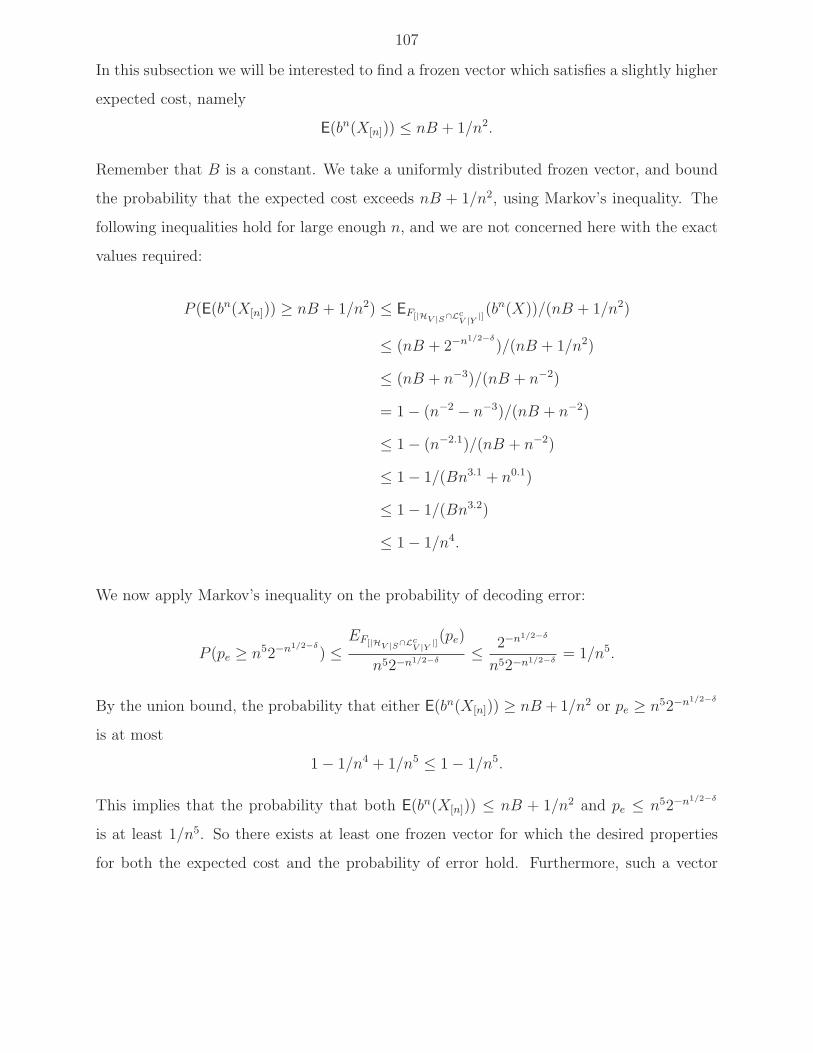
107

In this subsection we will be interested to find a frozen vector which satisfies a slightly higher

expected cost, namely

E(bn(X[n])) ≤ nB + 1/n2.

Remember that B is a constant. We take a uniformly distributed frozen vector, and bound

the probability that the expected cost exceeds nB + 1/n2, using Markov’s inequality. The

following inequalities hold for large enough n, and we are not concerned here with the exact

values required:

P (E(bn(X[n])) ≥ nB + 1/n2) ≤ EF[|HV |S∩LcV |Y

|](bn(X))/(nB + 1/n2)

≤ (nB + 2−n1/2−δ

)/(nB + 1/n2)

≤ (nB + n−3)/(nB + n−2)

= 1− (n−2 − n−3)/(nB + n−2)

≤ 1− (n−2.1)/(nB + n−2)

≤ 1− 1/(Bn3.1 + n0.1)

≤ 1− 1/(Bn3.2)

≤ 1− 1/n4.

We now apply Markov’s inequality on the probability of decoding error:

P (pe ≥ n52−n1/2−δ

) ≤EF[|HV |S∩Lc

V |Y|](pe)

n52−n1/2−δ≤ 2−n1/2−δ

n52−n1/2−δ= 1/n5.

By the union bound, the probability that either E(bn(X[n])) ≥ nB + 1/n2 or pe ≥ n52−n1/2−δ

is at most

1− 1/n4 + 1/n5 ≤ 1− 1/n5.

This implies that the probability that both E(bn(X[n])) ≤ nB + 1/n2 and pe ≤ n52−n1/2−δ

is at least 1/n5. So there exists at least one frozen vector for which the desired properties

for both the expected cost and the probability of error hold. Furthermore, such a vector

108

can be found by repeatedly selecting a frozen vector uniformly at random until the required

properties hold. The properties can be verified efficiently with close approximations by the

upgradation and degradation method proposed in [81]. The expected number of times until

a good vector is found is polynomial in the block length (at most n5). This completes the

proof of Theorem 5.7.

109

Part IV

Local Rank Modulation

110

Chapter 6

Rewriting with Gray Codes

The material in this chapter was published in [19,20].

6.1 Definitions and Notation

6.1.1 Local Rank Modulation

Assume we have a set of t flash memory cells which we number 0, 1, . . . , t−1. Let us considera sequence of t real-valued variables, c = (c0, c1, . . . , ct−1) ∈ R

t, where ci denotes the charge

level measured in the ith flash memory cell. We further assume ci 6= cj for all i 6= j. The

t variables induce a permutation fc ∈ St, where St denotes the set of all permutations over

[t] = {0, 1, 2, . . . , t− 1}. The permutation fc is defined as

fc(i) = |{j | cj < ci}| .

Thus, fc(i) is the rank of the ith cell in ascending order.

We now turn to consider a larger set of n ≥ t flash memory cells. Again, we have a

sequence of n variables, c = (c0, c1, . . . , cn−1) ∈ Rn where ci denotes the measured charge

level in the ith flash memory cell. We define a window of size t at position p to be

cp,t = (cp, cp+1, . . . , cp+t−1),

111

where the indices are taken modulo n, and also 0 ≤ p ≤ n−1, and 1 ≤ t ≤ n. We now define

the (s, t, n)-local rank-modulation (LRM) scheme, which we do by defining the demodulation

process. Let s ≤ t ≤ n be positive integers, with s|n. Given a sequence of n distinct

real-valued variables, c = (c0, c1, . . . , cn−1), the demodulation maps c to the sequence of n/s

permutations from St as follows:

fc = (fc0,t , fcs,t , fc2s,t , . . . , fcn−s,t). (6.1)

Loosely speaking, we scan the n variables using windows of size t positioned at multiples of

s and write down the permutations from St induced by the local views of the sequence.

In the context of flash-memory storage devices, we shall consider the n variables, c =

(c0, c1, . . . , cn−1), to be the charge-level readings from n flash cells. The demodulated se-

quence, fc, will stand for the original information which was stored in the n cells. This ap-

proach will serve as the main motivation for this chapter, as it was also for [19,45,46,82,85].

See Figure 6.1 for an example of a demodulation of a (3, 5, 12)-locally rank-modulated signal.

������������

����������������

����������������

���������������������������

���������������������������

������������

������������

��������

������������������

������������������

��������������

��������������

������������

������������

����������������

����������������

������������������

������������������

�������� ��

������

c0 = 5.00 c1 = 2.50 c2 = 4.25 c3 = 6.50 c4 = 4.00 c5 = 1.00 c6 = 1.50 c7 = 5.50 c8 = 6.00 c9 = 1.00 c10 = 4.00c11 = 1.50

Demodulation: fc = ([3, 0, 2, 4, 1], [4, 2, 0, 1, 3], [1, 3, 4, 0, 2], [0, 3, 1, 4, 2])Condensed factoradic: fc = ((3, 0, 1), (4, 2, 0), (1, 2, 2), (0, 2, 0))

Figure 6.1: Demodulating a (3, 5, 12)-locally rank-modulated signal.

112

We say a sequence f of n/s permutations over St is (s, t, n)-LRM realizable if there exists

c ∈ Rn such that f = fc, i.e., it is the demodulated sequence of c under the (s, t, n)-LRM

scheme. Except for the degenerate case of s = t, not every sequence is realizable. For

example, if s < t and fci·s,t is the identity permutation (i.e., fci·s,t(i) = i), then for all

1 ≤ j < n we have cj < cj+1, but also cn < c1, which is impossible.

We denote the set of all (s, t, n)-LRM realizable permutation sequences as R(s, t, n). Ina later part of this section, we show that the number of states representable by an (s, t, n)-

LRM scheme, i.e., the size of R(s, t, n), is roughly (t · (t− 1) · ... · (t− s+ 1))n/s (this fact is

also stated in [85]).

While any f ∈ R(s, t, n) may be represented as a sequence of n/s permutations over

St, a more succinct representation is possible based on the (mixed-radix) factoradic notation

system (see [52] for the earliest-known definition, and [45] for a related use): We can represent

any permutation f = [f(0), . . . , f(t− 1)] ∈ St with a sequence of digits dt−1, dt−2, . . . , d1, d0

(note the reversed order of indices), where dt−1−i ∈ Zt−i, and dt−1−i counts the number of

entries f(j) for j > i which are of value lower than f(i), i.e.,

dt−1−i = |{j > i | cj < ci}|.

We call dt−1 the most-significant digit and d0 the least-significant digit. If f = fc for some

c ∈ Rt, then the factoradic representation is easily seen to be equivalent to counting the

number of cells to the right of the ith cell which are with lower charge levels.

Continuing with the succinct representation, we now contend that due to the overlap

between local views, we can represent each of the local permutations fci·s,t using only the s

most-significant digits in their factoradic notation. We denote this (partial) representation

as fci·s,t and call it the condensed factoradic representation. Accordingly, we define,

fc = (fc0,t , fcs,t , fc2s,t , . . . , fcn−s,t),

and the set of all such presentations as R(s, t, n). Thus, for example, the configuration of

113

Figure 6.1 would be represented by ((3, 0, 1), (4, 2, 0), (1, 2, 2), (0, 2, 0)). Since throughout the

rest of the chapter we shall deal with the condensed factoradic representation only, we omit

from now on the term “condensed”.

Lemma 6.1: For all 1 ≤ s ≤ t ≤ n,

∣

∣R(s, t, n)∣

∣ ≤ |R(s, t, n)| ≤ (t− s)! ·(

t!

(t− s)!

)ns

.

Proof: As R(s, t, n) = {fc | fc ∈ R(s, t, n)} we have that∣

∣R(s, t, n)∣

∣ ≤ |R(s, t, n)|. For theupper bound, assume we fix the permutation induced by the first t− s cells, where there are

(t− s)! ways of doing so. It follows that there are at most t!/(t− s)! ways of choosing fcn−s,t ,

and then the same bound on the number of ways of choosing fcn−2s,t , and continuing all the

way up to fc0,t we obtain the desired bound. �

When s = t = n, the (n, n, n)-LRM scheme degenerates into a single permutation from

Sn. This was the case in most of the previous works using permutations for modulation

purposes. A slightly more general case, s = t < n was discussed by Ferreira et al. [24] in

the context of permutation trellis codes, where a binary codeword was translated tuple-wise

into a sequence of permutations with no overlap between the tuples. An even more general

case was defined by Wang et al. [85] (though in a slightly different manner where indices

are not taken modulo n, i.e., with no wrap-around). In [85], the sequence of permutations

was studied under a charge-difference constraint called bounded rank-modulation, and mostly

with parameters s = t− 1, i.e., an overlap of one position between adjacent windows.

6.1.2 Gray Codes

A Gray code, G, is a sequence of distinct states (codewords), G = g0, g1, . . . , gN−1, from an

ambient state space, gi ∈ S, such that adjacent states in the sequence differ by a “small”

change. What constitutes a “small” change usually depends on the code’s application.

Since we are interested in building Gray codes for flash memory devices with the (s, t, n)-

LRM scheme, the ambient space is R(s, t, n), which is the set of all realizable sequences

114

������

������

������������������

������������������

������������

������������

������

������

��������������������

��������������������

��������������

��������������

����������

����������

����������������

����������������

������������

������������

������

������

������

������

����������������

����������������

����������������

����������������

c′0 = 5.00 c′1 = 2.50 c′2 = 4.25 c′3 = 6.50 c′4 = 4.00 c′5 = 1.00 c′6 = 1.50 c′7 = 5.50 c′8 = 6.00 c′9 = 6.25 c′10 = 4.00 c′11 = 1.50

Demodulation: fc′ = ([3, 0, 2, 4, 1], [4, 2, 0, 1, 3], [0, 2, 3, 4, 1], [4, 2, 0, 3, 1])Condensed factoradic: fc′ = ((3, 0, 1), (4, 2, 0), (0, 1, 1), (4, 2, 0))

Figure 6.2: A “push-to-the-top” operation performed on the 9th cell.

under (s, t, n)-LRM.

The transition between adjacent states in the Gray code is directly motivated by the

flash memory application, and was first described and used in [45]. This transition is the

“push-to-the-top” operation, which takes a single flash cell and raises its charge level above

all others.

In our case, however, since we are considering a local rank-modulation scheme, the “push-

to-the-top” operation merely raises the charge level of the selected cell above those cells which

are comparable with it.

In Figure 6.2 we see the example signal of Figure 6.1 after a “push-to-the-top” operation

performed on the 9th cell. The cells participating with the 9th cell in local permutations are

6, 7, 8, 10, 11, 0, and 1, i.e., from cell 6 to cell 1 with wrap-around. Thus, the charge level of

the 9th cell was pushed above that of cells 6 through 1 (with wrap-around). We do note that

the new charge level of the 9th cell is not above that of all other cells since the 3rd cell still

has a higher level. However, the 3rd cell is incomparable (i.e., does not participate in a local

115

permutation) with the 9th cell. Figure 6.2 also shows the demodulation and condensed fac-

toradic representation of the new configuration. By comparing with Figure 6.1, we note that

a single “push-to-the-top” operation can change several digits in the demodulated sequence

and in the factoradic notation.

We now provide a precise definition of the “push-to-the-top” operation in the local

rank-modulation scheme. Assume we have n flash memory cells with charge levels c =

(c0, . . . , cn−1) ∈ Rn. We say cell j is comparable with cell j′ if they both participate in some

window together. We shall denote these cells as the cells numbered l(j), l(j) + 1, . . . , r(j)

where one can easily verify that

l(j) = s

⌈

j − t+ 1

s

⌉

mod n,

r(j) =

(

s

⌊

j

s

⌋

+ (t− 1)

)

mod n.

We note that the indices l(j), l(j) + 1, . . . , r(j) should be taken modulo n. Continuing the

example of Figure 6.2, for s = 3 and t = 5 we have l(8) = 3⌈(8 − 5 + 1)/3⌉ = 6 and

r(10) = (3⌊10/3⌋+5− 1) ≡ 1 (mod 12), i.e., the left-most cell comparable with cell 8 is cell

6, while the right-most cell comparable with cell 10 is cell 1.

A “push-to-the-top” operation performed on cell j changes the cell levels to

c′ = (c′0, . . . , c′n−1) ∈ R

n defined by

c′i =

ci i 6= j,

max{

cl(i), . . . , cr(i)}

+ ǫ i = j,

where ǫ > 0 denotes a small charge difference which is a parameter of the physical charge-

placement mechanism. Namely, the charge level of cell j is pushed above the charge levels

of cells comparable with it.

We can now move from the physical level to the logical level of the demodulated signal.

With the above notation, c′ was achieved from c by a “push-to-the-top” operation on cell j.

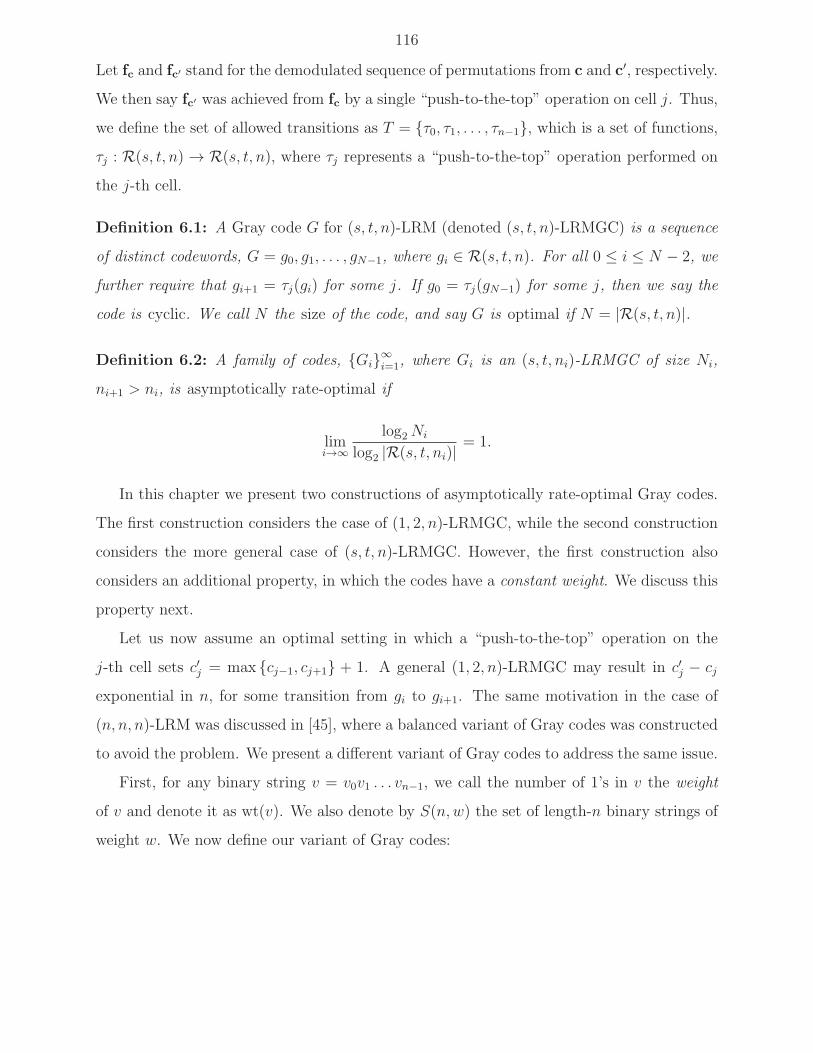
116

Let fc and fc′ stand for the demodulated sequence of permutations from c and c′, respectively.

We then say fc′ was achieved from fc by a single “push-to-the-top” operation on cell j. Thus,

we define the set of allowed transitions as T = {τ0, τ1, . . . , τn−1}, which is a set of functions,

τj : R(s, t, n)→ R(s, t, n), where τj represents a “push-to-the-top” operation performed on

the j-th cell.

Definition 6.1: A Gray code G for (s, t, n)-LRM (denoted (s, t, n)-LRMGC) is a sequence

of distinct codewords, G = g0, g1, . . . , gN−1, where gi ∈ R(s, t, n). For all 0 ≤ i ≤ N − 2, we

further require that gi+1 = τj(gi) for some j. If g0 = τj(gN−1) for some j, then we say the

code is cyclic. We call N the size of the code, and say G is optimal if N = |R(s, t, n)|.

Definition 6.2: A family of codes, {Gi}∞i=1, where Gi is an (s, t, ni)-LRMGC of size Ni,

ni+1 > ni, is asymptotically rate-optimal if

limi→∞

log2 Ni

log2 |R(s, t, ni)|= 1.

In this chapter we present two constructions of asymptotically rate-optimal Gray codes.

The first construction considers the case of (1, 2, n)-LRMGC, while the second construction

considers the more general case of (s, t, n)-LRMGC. However, the first construction also

considers an additional property, in which the codes have a constant weight. We discuss this

property next.

Let us now assume an optimal setting in which a “push-to-the-top” operation on the

j-th cell sets c′j = max {cj−1, cj+1} + 1. A general (1, 2, n)-LRMGC may result in c′j − cj

exponential in n, for some transition from gi to gi+1. The same motivation in the case of

(n, n, n)-LRM was discussed in [45], where a balanced variant of Gray codes was constructed

to avoid the problem. We present a different variant of Gray codes to address the same issue.

First, for any binary string v = v0v1 . . . vn−1, we call the number of 1’s in v the weight

of v and denote it as wt(v). We also denote by S(n,w) the set of length-n binary strings of

weight w. We now define our variant of Gray codes:

117

Definition 6.3: A constant-weight Gray code for (1, 2, n)-LRM (denoted (1, 2, n;w)-LRMGC),

G = g0, g1, . . . , gN−1, is a Gray code for (1, 2, n)-LRM for which gi ∈ S(n,w) for all

0 ≤ i ≤ N − 1.

Definition 6.4: Let G be a (1, 2, n;w)-LRMGC of size N . We define the rate of the code

as R(G) = log2 Nn

. The efficiency of G is defined as Eff(G) = N/(

nw

)

. If Eff(G) = 1 then we

say G is optimal. If Eff(G) = 1 − o(1), where o(1) denotes a function that tends to 0 as

n→∞, then we say G is asymptotically optimal.

The transitions between adjacent states in the constant-weight variant take on a very

simple form: a window of size 2 in gi which contains 10 is transformed in gi+1 into 01, i.e.,

“pushing” a logical 1 a single place to the right. Since we are interested in creating cyclic

counters, we will be interested in cyclic Gray codes. An example of a cyclic optimal Gray

code is given in Table 6.1.

Table 6.1: A cyclic optimal (1, 2, 5; 2)-LRMGC (The changed positions are underlined.)

1 1 0 0 01 0 1 0 00 1 1 0 00 1 0 1 00 0 1 1 00 0 1 0 10 0 0 1 11 0 0 1 01 0 0 0 10 1 0 0 1

It should be noted that Gray codes with a weaker restriction, allowing a 01 to be changed

into 10 and also 10 to be changed back into 01, i.e., a 1 may be pushed either to the right

or to the left, have been studied in the past [6, 9, 15, 38, 71].

We can show that under the constant-weight restriction, for any “push-to-the-top” oper-

ation,

c′j − cj ≤⌈

max {w, n− w}min {w, n− w}

⌉

.

118

This is done by first assuming 2w ≤ n, or else we flip all the bits and reverse the codewords.

We will only use integer charge levels, and thus for any codeword, gi, wt(gi) = w, we can

find a realization by setting cj+1− cj = 1 if gi,j = 0, and cj+1− cj = −[(n−w)/w] if gi,j = 1,

where [·] denotes either ⌊·⌋ or ⌈·⌉.It is now easily shown by induction that a “push-to-the-top” operation on the j-th cell

preserves charge-level differences between adjacent cells and only rearranges their order: by

the induction hypothesis, initially we have cj − cj−1 = −[(n−w)/w] and cj+1− cj = 1. The

“push-to-the-top” operation sets c′j = max {cj−1, cj+1}+1 = cj−1 +1 and then c′j − cj−1 = 1

and cj+1 − c′j = −[(n− w)/w].

6.2 Constant-Weight Gray Codes for (1, 2, n)-LRM

In this section we construct (1, 2, n)-LRMGCs with rates asymptotically tending to 1, and

weight asymptotically half the length, thus having asymptotically-optimal charge difference

between adjacent cells. Our construction has the following intuitive flavor. We start by

partitioning the n flash cells into about√n blocks, each block of size about

√n, treating

each block of cells as a single character in a large alphabet, say {0, 1, . . . , t− 1} for t ≃ 2√n.

Roughly speaking, by this operation, we have reduced the problem of finding a Gray code

over {0, 1}n into an outer Gray-like code over {0, 1, . . . , t− 1}√n. Several Gray codes of rate

1 exist over large alphabets, however, not any outer code will suffice in our setting. Primarily,

it is crucial that we may move from state to state in the outer code using our elementary

pairwise “push-to-the-top” operations. Moreover, in doing so, we must guarantee that flash

cell values obtained between a single representation of the outer codeword and its successor

are unique. We achieve these goals using an outer Gray code based on de-Bruijn sequences.

In such codes, the location of the character that changes between subsequent codewords over

goes a cyclic shift. This cyclic location change between subsequent codewords lends itself

very naturally to our cyclic “push-to-the-top” operations. Combining this with additional

ideas that guarantee distinct cell values (of constant weight) in transition between outer

119

codewords, we obtain our construction.

Construction 6.1: Fix a positive integer k. Let {v0, v1, . . . , vt−1} be a set of t distinct

binary vectors of length m+ 2 and weight w + 2 such that the first and last bit of each vi is

1. We also denote L = lcm(k + 2, tk).

The next required ingredient in the construction is a de-Bruijn sequence of order k over the

alphabet {0, 1, . . . , t− 1}. The sequence is of period tk and we denote it by s0, s1, . . . , stk−1.

We remind the reader that windows of size k in the sequence, i.e., si, si+1, . . . , si+k−1, with

indices taken modulo tk, are all distinct. Such sequences can always be constructed (for

example, see [31]).

We now construct the sequence g0, g1, . . . , gL−1 of L binary vectors of length (k+2)(m+2)

and weight (k+1)(w+2). Each vector is formed by a concatenation of k+2 blocks of length

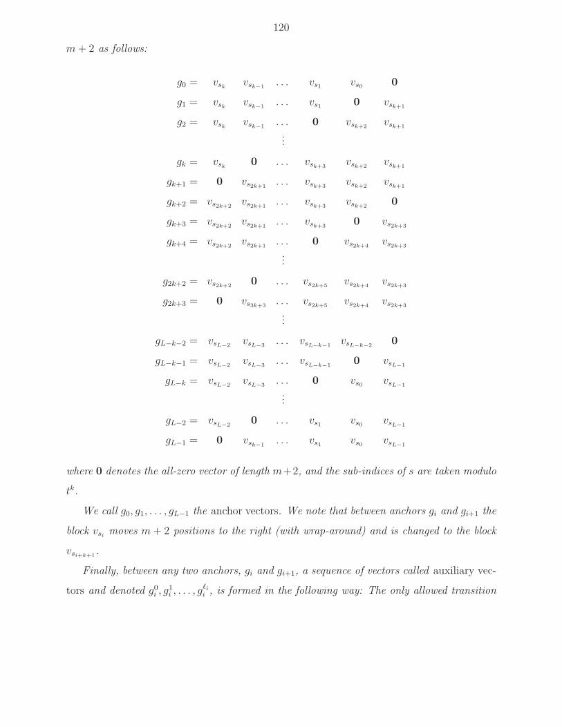
120

m+ 2 as follows:

g0 = vsk vsk−1. . . vs1 vs0 0

g1 = vsk vsk−1. . . vs1 0 vsk+1

g2 = vsk vsk−1. . . 0 vsk+2

vsk+1

...

gk = vsk 0 . . . vsk+3vsk+2

vsk+1

gk+1 = 0 vs2k+1. . . vsk+3

vsk+2vsk+1

gk+2 = vs2k+2vs2k+1

. . . vsk+3vsk+2

0

gk+3 = vs2k+2vs2k+1

. . . vsk+30 vs2k+3

gk+4 = vs2k+2vs2k+1

. . . 0 vs2k+4vs2k+3

...

g2k+2 = vs2k+20 . . . vs2k+5

vs2k+4vs2k+3

g2k+3 = 0 vs3k+3. . . vs2k+5

vs2k+4vs2k+3

...

gL−k−2 = vsL−2vsL−3

. . . vsL−k−1vsL−k−2

0

gL−k−1 = vsL−2vsL−3

. . . vsL−k−10 vsL−1

gL−k = vsL−2vsL−3

. . . 0 vs0 vsL−1

...

gL−2 = vsL−20 . . . vs1 vs0 vsL−1

gL−1 = 0 vsk−1. . . vs1 vs0 vsL−1

where 0 denotes the all-zero vector of length m+2, and the sub-indices of s are taken modulo

tk.

We call g0, g1, . . . , gL−1 the anchor vectors. We note that between anchors gi and gi+1 the

block vsi moves m+ 2 positions to the right (with wrap-around) and is changed to the block

vsi+k+1.

Finally, between any two anchors, gi and gi+1, a sequence of vectors called auxiliary vec-

tors and denoted g0i , g1i , . . . , g

ℓii , is formed in the following way: The only allowed transition

121

is a 10 changed into a 01. First the rightmost 1 in the block vsi is moved to the right, step by

step, to the position of the rightmost 1 in vsi+k+1. The process then repeats with a sequence

of transitions moving the second-from-right 1 in vsi to the position of the second-from-right

1 in vsi+k+1, and so on, until vsi is moved one block to the right and changed into vsi+k+1

(see

Example 6.1). The resulting list of anchor vectors and, in between them, auxiliary vectors,

is the constructed code.

Example 6.1: Let us take a very simple case of k = 1, m = 3, w = 2, and t = 3, with

s0 = 0, s1 = 1, and s2 = 2, and then v0 = 11101, v1 = 11011, and v2 = 10111. The list of

anchors is

g0 = 11011 11101 00000

g1 = 11011 00000 10111

g2 = 00000 11101 10111

and, for example, the transition between g0 and g1 is shown in Table 6.2 (the changed posi-

tions are underlined).

Theorem 6.1: The code constructed in Construction 6.1 is a cyclic (1, 2, (k+2)(m+2); (k+

1)(w + 2))-LRMGC of size

N = L(w + 2)(m+ 2) = lcm(tk, k + 2) · (w + 2) · (m+ 2).

The proof of Theorem 6.1 requires the following definition:

Definition 6.5: For any v = v0v1 . . . vn−1 ∈ S(n,w), we define the first moment of v as

χ(v) =n−1∑

j=0

j · vj (6.2)

and the color of v as χ(v) mod n.

Proof (of Theorem 6.1): That the code contains only valid transitions is evident by the

construction method. We need to show that all the constructed codewords are distinct,

122

Table 6.2: The transitions between anchors in Example 6.1.

g0 = 11011 11101 00000g00 = 11011 11100 10000g10 = 11011 11100 01000g20 = 11011 11100 00100g30 = 11011 11100 00010g40 = 11011 11100 00001g50 = 11011 11010 00001g60 = 11011 11001 00001g70 = 11011 11000 10001g80 = 11011 11000 01001g90 = 11011 11000 00101g100 = 11011 11000 00011g110 = 11011 10100 00011g120 = 11011 10010 00011g130 = 11011 10001 00011g140 = 11011 10000 10011g150 = 11011 10000 01011g160 = 11011 10000 00111g170 = 11011 01000 00111g180 = 11011 00100 00111g190 = 11011 00010 00111g200 = 11011 00001 00111g1 = 11011 00000 10111

123

which we do with the following reasoning: consider some constructed codeword g of length

(k + 2)(m+ 2) and weight (k + 1)(w + 2). Deciding whether g is an anchor is simple, since

only anchors have k + 1 blocks beginning and ending with a 1, and the remaining block a

0. By our choice of L, all anchors are distinct since they contain windows of size k+ 1 from

a de-Bruijn sequence of order k, each window appearing in (k + 2)/ gcd(k + 2, tk) distinct

cyclic shifts (which are easily distinguishable by the position of the 0 block). It then follows

that if g is indeed an anchor it appears only once in the code.

Assume we discover g is an auxiliary vector. Again, by construction, all auxiliary vectors

between gi and gi+1 have k fixed blocks. Looking at g, an auxiliary vector, exactly k blocks

are of weight w+2 while the other two blocks have weight strictly below w+2. The blocks of

weight w+2, by construction, form a window of size k from a de-Bruijn sequence of order k

starting at si, and so their content and position uniquely identify between which two anchors

g lies.

Finally, all the auxiliary vectors between adjacent anchors gi and gi+1 are easily seen to be

distinct. Thus, given a codeword g from the constructed code, there is exactly one position

in the sequence of generated codewords which equals g, and so all generated codewords are

distinct.

To complete the proof we need to calculate the size N . There are exactly L anchors.

Given an anchor gi, the number of steps in the transition to gi+1 may be readily verified to

be (w+2)(m+2)+χ(gi+1)−χ(gi), where χ(·) is the first moment function defined in (6.2).

Thus,

N =L−1∑

i=0

((w + 2)(m+ 2) + χ(gi+1)− χ(gi))

= L(w + 2)(m+ 2)

as claimed. As a final note, the choice of L is easily seen to ensure the resulting code is

cyclic. �

124

We mention in passing that the proof of Theorem 6.1 hints at efficient encoding and

decoding procedures, provided other efficient encoding and decoding procedures exist for

de-Bruijn sequences. Examples of such procedures may be found in [61,84].

We now turn to show the main claim of the section.

Corollary 6.1: There exists an infinite family {Gi}∞i=1 of cyclic (1, 2, ni;wi)-LRMGCs, ni+1 >

ni for all i, for which limi→∞ R(Gi) = 1, and limi→∞wi

ni= 1

2.

Proof: For the code Gi, set w = i, and k = m = 2i (i.e., ni = (2i + 2)2 and wi =

(2i + 1)(i + 2)) and apply Theorem 6.1 with t =(

2ii

)

. The size, Ni, of the code Gi, is

bounded by(

2i

i

)2i

(i+ 2)(2i+ 2) ≤ Ni ≤(

2i

i

)2i

(i+ 2)(2i+ 2)2

since(

2i

i

)2i

≤ lcm

(

(

2i

i

)2i

, 2i+ 2

)

≤(

2i

i

)2i

(2i+ 2).

It is well known (see for example [57], p. 309) that for any 0 < λ < 1, assuming λℓ is an

integer,1

√

8ℓλ(1− λ)2ℓH(λ) ≤

(

ℓ

λℓ

)

≤ 1√

2ℓλ(1− λ)2ℓH(λ)

where H(·) is the binary entropy function. Since H(1/2) = 1, it now easily follows that

limi→∞

R(Gi) = 1, limi→∞

wi

ni

=1

2.

�

If needed, we can achieve lower asymptotic rates by setting w = λm for some rational

0 < λ < 1, λ 6= 1/2.

6.3 Gray Codes for (s, t, n)-LRM

In this section we present efficiently encodable and decodable asymptotically-rate-optimal

Gray codes for (s, t, n)-LRM. A rough description of the proposed construction follows.

125

First we partition the n cells into m blocks, each containing n/m cells. To simplify the

presentation we set n = m2, implying that we have m blocks, each of size m. Denote the

cells in block i by ci. For each block ci we will use the factoradic representation fci to

represent permutations, without wrap-around at the block level (the wrap-around is only for

the entire codeword). Namely, each and every block can be thought of as an element of an

alphabet Σ = {v0, . . . , vV−1} of a size denoted by V .

Now, consider any De-Bruijn sequence S of order m−1 over Σ (of period V m−1). Namely,

S will consist of a sequence of V m−1 elements vs0 , vs1 , . . . , vsV m−1−1over Σ such that the

subsequences vsi , . . . , vsi+m−2of S cover all (m− 1)-tuples of Σ exactly once, sub-indices of

s are taken modulo V m−1. We shall conveniently choose Σ = ZV . Such sequences S exist,

e.g., [31].

The construction of the Gray code G will have two phases. First we construct so-called

anchor elements in G, denoted as G = {g0, . . . , gL−1}. The elements of G will consist of a

cyclic Gray code over Σm. That is, the difference between each gi and gi+1 in G will be in

only one out of the m characters (from Σ) in gi. Specifically, the code G will be derived from

the De-Bruijn sequence S as follows: we set g0 to be the first m elements of S, and in the

transition from gi to gi+1 we change vsi to vsi+m. The code G is detailed below:

g0 = vsm−1 vsm−2 . . . vs1 vs0

g1 = vsm−1 vsm−2 . . . vs1 vsm

g2 = vsm−1 vsm−2 . . . vsm+1 vsm...

gL−2 = vsL−1vsL−2

. . . vs1 vs0

gL−1 = vsL−1vsm−2 . . . vs1 vs0 ,

where L = lcm(m,V m−1), the sub-indices of s are taken modulo V m−1, and the underline is

an imaginary marking distinguishing the block which is about to change.

With the imaginary marking of the underline, the code G is clearly a Gray code over

Σm due to the properties of the De-Bruijn sequence S. However G is not a Gray code over

126

R(s, t, n), as the transitions between the anchors gi and gi+1 require changing the entries

of an entire block, which may involve many push-to-the-top operations. We thus refine G

by adding additional elements between each pair of adjacent anchors from G that allow us

to move from the block configuration in gi to that in gi+1 by a series of push-to-the-top

operations.

Each block is eventually represented in factoradic notation by a sequence of digits. For

the construction to work, it is crucial to be able to identify, for each element in G, which

block is in the process of being changed. To this end, and for other technical reasons, we

will add some auxiliary digits to each block (by adding auxiliary flash memory cells). These

digits are referred to as non-information digits. Loosely speaking, in each block of size m

the last t + 1 digits (approximately1) will be non information digits. The last 2 digits will

be used to mark which block is being currently changed, while the t− 1 digits before them

will act as a buffer zone that allows the successful transformation between anchors. In our

setting, the t + 1 non-information digits will be negligible with respect to the remaining

m− (t+ 1) information digits, allowing the code G to have asymptotically optimal rate.

Construction 6.2: We consider the (s, t, n)-LRM scheme, where

n = m2, m ≥ t+ 2, s | m.

Let {v0, v1, . . . , vV−1} be a set of V distinct mixed-radix vectors of length m. Each vector

vi is representing m/s local permutations, where each permutation is represented by the s

most-significant digits of its factoradic notation. Therefore,

vi ∈(

Zt × Zt−1 × · · · × Zt−(s−1)

)m/s.

Let us denote

δ =

⌈

t+ 2

s

⌉

− 1.

1For the exact value see Construction 6.2.

127

The values of the last sδ digits (that represent the last δ local permutations) of each vi do

not play a role in the representation of the stored data and are called non-information digits.

By abuse of notation, two vectors agreeing on the first m− sδ digits will be said to represent

the same value. Furthermore, when a block is said to represent some value vi, we mean that

its first m− sδ digits agree with those of vi. Therefore, we set

V =

(

t!

(t− s)!

)ms−δ

.

We also denote L = lcm(m,V m−1).

Let S be a De-Bruijn sequence of order m− 1 over the alphabet ZV ,

S = s0, s1, . . . , sV m−1−1,

i.e., S is of length V m−1 and si ∈ ZV . The Gray code G of anchor vectors is a sequence

G = g0, g1, . . . , gL−1

of L mixed-radix vectors of length n = m2. Each vector is formed by a concatenation of m

blocks of length m. For k ∈ [m], we say that block k corresponds to the cells with indices

km, km+ 1, . . . , (k + 1)m− 1. We set g0 to be the concatenation of the first m elements of

S, such that for each k ∈ [m], block k represent the vector vsm−1−k:

g0 = vsm−1vsm−2 . . . vs1vs0 .

Between the anchors gi and gi+1, the block that represents the vector vsi is transformed into

128

the vector vsi+m. The resulting Gray code G of anchor vectors is therefore

g0 = vsm−1 vsm−2 . . . vs1 vs0

g1 = vsm−1 vsm−2 . . . vs1 vsm

g2 = vsm−1 vsm−2 . . . vsm+1 vsm...

gL−2 = vsL−1vsL−2

. . . vs1 vs0

gL−1 = vsL−1vsm−2 . . . vs1 vs0 ,

where the underline denotes the block that is about to change in the transition to the following

anchor vector.

Within each of the m blocks comprising any single anchor, the (m − 2)nd digit (the

next-to-last digit – a non-information digit) corresponds to a cell that is pushed-to-the-top

in all blocks except for the “underlined” block (i.e., the block which is about to change). For

brevity, we call this digit the underlined digit. In the underlined block, the (m− 1)th digit is

pushed-to-the-top. All remaining non-information digits are initialized to be of value 0.

Between any two anchors, gi and gi+1, a sequence of vectors called auxiliary vectors and

denoted g0i , g1i , . . . , g

ℓii , is formed by a sequence of push-to-the-top operations on the cells of

the changing block. The auxiliary vectors are determined by Algorithm 6.1 described shortly.

Thus, the entire Gray code G constructed is given by the sequence

g0, g00, g10, . . . gℓ00 ,

g1, g01, g11, . . . gℓ11 ,...

gL−1, g0L−1, g1L−1, . . . gℓL−1

L−1 .

In what follows we present Algorithm 6.1 that specifies the sequence g0i , g1i , . . . , g

ℓii that

allows us to move from anchor state gi to state gi+1. As gi and gi+1 differ only in a single

block (and this block is changed from representing the value vsi to vsi+m), it holds that gji

129

and gj′

i will differ only in the block in which gi and gi+1 differ. Thus, it suffices to define in

Algorithm 6.1 how to change a block of length m with cell values that represent vsi into a

block that represents vsi+musing push-to-the-top operations. However, we call the attention

of the reader to the fact that while the change in represented value affects only one block

(denoted as block k), for administrative reasons, in block k − 1 (modulo m) we also push a

non-information cell. The inputs of Algorithm 6.1 are the vector vsi+mand the corresponding

cell configuration (ckm, ckm+1, . . . , c(k+1)m−1), and its output is the order in which those cells

are pushed in order to transform the vector represented in block k into vsi+m. Algorithm

6.1 also ensures that the underlined digits of blocks k and k− 1 (modulo m) of an auxiliary

vector are both not of maximal value (among the cells with which they share a window).

This allows to identify whether the vector is an anchor vector or an auxiliary one. Assuming

that

(r0, r1, . . . , rm−1) ∈(

Zt × Zt−1 × · · · × Zt−(s−1)

)m/s

represents the value vℓ, then we say that the jth digit of vℓ is

vℓ(j) =

rj 0 ≤ j < m− sδ

0 otherwise,

i.e., we always force a 0 for the non-information digits. Finally, we restrict l(·) and r(·) bydefining

l′(j) =

l(j) 0 ≤ l(j) ≤ m− 3

0 otherwise

r′(j) =

r(j) 0 ≤ r(j) ≤ m− 3

m− 3 otherwise.

Algorithm 6.1 is strongly based on the factoradic representation of vsi+m. Let vsi+m

(j)

be the jth entry in this representation. Namely, if c = (c0, . . . , cm−1) is a cell configuration

130

Algorithm 6.1 Transform block k of configuration fc from vsi to vsi+m

Input: current cell configuration fc, block number k, new block value vsi+m

Output: new cell configuration fc′

Push cell m− 1 (the last cell) in block k − 1 (modulo m).aj ⇐ 0 for all j = 0, 1, . . . ,m− 3j ⇐ 0repeat

if vsi+m(j) =

r′(j)∑

i=j+1

ai and aj = 0 then

if ckm+j ≤ maxl′(j)≤j′≤r′(j),aj′=1

ckm+j′ then

Push the jth cell in block k (the cell in position km+ j).end if

aj ⇐ 1j ⇐ l′(j)

else

j ⇐ j + 1end if

until j = m− 2Push cell m− 2 (the next-to-last cell) in block k.Output the resulting cell configuration fc′ .

that corresponds to vsi+m, then for each index j ∈ [m] we let vsi+m

(j) denote the number

of entries in the window corresponding to j that are in a larger position than j and are of

value lower than cj. Roughly speaking, to obtain such a configuration c, Algorithm 6.1, for

j ∈ [m], marks each cell cj in c after exactly vsi+m(j) cells in positions larger than j (and

participating in the window corresponding to j) have been marked. Here, in order to keep

track of which cells should not be pushed anymore, we save an array of bits aj for each cell

in the block (initialized to 0), indicating whether the cell cj should not be pushed anymore.

If aj = 1, we say that cell j is marked. Furthermore, when the cell is marked, it is also

pushed-to-the-top if its value is lower than that of a cell that shares a window with it and

is already marked (the value comparison can be inferred from fc). Since each time a cell is

changed it is pushed-to-the-top, this will ensure that the resulting cell configuration c will

have a factoradic representation corresponding to vsi+m.

We note that in order to be able to decode a state, we need to have some way of knowing

131

which block is being currently changed, i.e., the imaginary underline in the anchor. We use

the last two cells of each block for that purpose as described in the example below.

Example 6.2: Let us consider the case of (1, 2, 16)-LRM, i.e., s = 1, t = 2, m = 4, and

n = m2 = 16. Thus,

δ =

⌈

t+ 2

s

⌉

− 1 =

⌈

2 + 2

1

⌉

− 1 = 3,

and so in each block, the last sδ = 3 digits are non-information digits, leaving only the first

digit in each block to be an information digit.

According to the construction we set

V =

(

t!

(t− s)!

)ms−δ

=

(

2!

(2− 1)!

) 41−3

= 2.

We therefore take a De-Bruijn sequence of order 3 and alphabet of size 2,

S = 0, 0, 0, 1, 0, 1, 1, 1.

The list of anchors is

g0 = 1010 0010 0010 0000

g1 = 1010 0010 0000 0010

g2 = 1010 0000 1010 0010

g3 = 1000 1010 1010 0010

g4 = 1010 1010 1010 0000

g5 = 1010 1010 1000 0010

g6 = 1010 1000 0010 0010

g7 = 1000 0010 0010 0010

The bold bit (the leftmost bit in each group of four) denotes the information bit, while the

rest are non-information bits. The underlined vectors are easily recognizable by the next-to-

rightmost (next-to-last) bit being 0.

Notice that in this example the information bit is dominated in size by the remaining bits

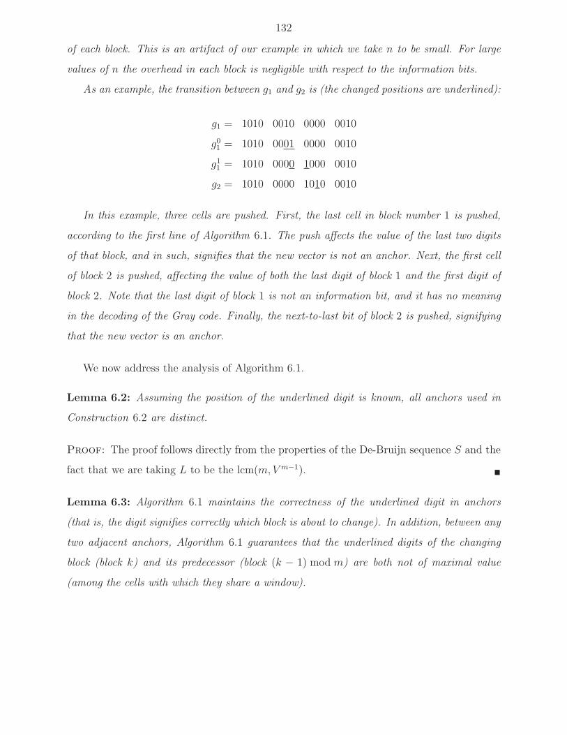
132

of each block. This is an artifact of our example in which we take n to be small. For large

values of n the overhead in each block is negligible with respect to the information bits.

As an example, the transition between g1 and g2 is (the changed positions are underlined):

g1 = 1010 0010 0000 0010

g01 = 1010 0001 0000 0010

g11 = 1010 0000 1000 0010

g2 = 1010 0000 1010 0010

In this example, three cells are pushed. First, the last cell in block number 1 is pushed,

according to the first line of Algorithm 6.1. The push affects the value of the last two digits

of that block, and in such, signifies that the new vector is not an anchor. Next, the first cell

of block 2 is pushed, affecting the value of both the last digit of block 1 and the first digit of

block 2. Note that the last digit of block 1 is not an information bit, and it has no meaning

in the decoding of the Gray code. Finally, the next-to-last bit of block 2 is pushed, signifying

that the new vector is an anchor.

We now address the analysis of Algorithm 6.1.

Lemma 6.2: Assuming the position of the underlined digit is known, all anchors used in

Construction 6.2 are distinct.

Proof: The proof follows directly from the properties of the De-Bruijn sequence S and the

fact that we are taking L to be the lcm(m,V m−1). �

Lemma 6.3: Algorithm 6.1 maintains the correctness of the underlined digit in anchors

(that is, the digit signifies correctly which block is about to change). In addition, between any

two adjacent anchors, Algorithm 6.1 guarantees that the underlined digits of the changing

block (block k) and its predecessor (block (k − 1) mod m) are both not of maximal value

(among the cells with which they share a window).

133

Proof: The proof is by induction. The base case follows from the construction of the first

anchor element g0. Assume gi satisfies the inductive claim. When applying Algorithm 6.1

to move from anchor gi to gi+1, we start by pushing the last cell of block k− 1. This implies

that the value of the underlined cell in both block k and block k−1 (modulo m) are now not

maximal. This state of affairs remains until the end of Algorithm 6.1, in which we push the

next-to-the last cell in the changed block (block k). At that point in time, the underlined

cell in the changed block obtains its maximal value, while block k− 1 (that is to be changed

in the next application of Algorithm 6.1) is of non-maximal value. All the other underlined

cells remain unchanged throughout the execution of Algorithm 6.1. �

Lemma 6.4: All words in the code G are distinct.

Proof: First, remember that the words in G are permutation sequences, while the construc-

tion is using the factoradic notation. However, different factoradic vectors always correspond

to different permutation sequences, and thus it is enough to show that the factoradic vectors

are distinct. Next, by Lemmas 6.2 and 6.3, we know that all of the anchors in Construc-

tion 6.2 are distinct. It is left to show that adding the auxiliary vectors resulting from

Algorithm 6.1, G remains a Gray code. It is easily seen that a non-anchor codeword can

never be mistaken for an anchor, and that due to the De-Bruijn sequence, two auxiliary

vectors gji and gj′

i′ can never be the same when i 6= i′.

Thus, it suffices to focus only on the block being changed. In order to show that every

word generated by Algorithm 6.1 in a single execution is distinct, we will show that every cell

configuration we encounter will never be visited again. Specifically, given a configuration,

we let j be the next cell that will be pushed. Since cell j is going to be pushed, there exists

a cell j′ such that cj < cj′ and aj′ = 1. After the push, cj > cj′ . But since aj′ = 1, cell j′

will not be pushed anymore, and thus in all future configurations cell j will be higher than

cell j′. Therefore all future configurations will differ from the initial one. �

Lemma 6.5: Algorithm 6.1 terminates, and when it does, all of the cells are marked exactly

once.

134

Proof: The index j is incremented by 1 in the algorithm’s loop, unless a cell is marked.

Since a cell cannot be marked more than once, the algorithm must terminate.

For each non-information digit index j′ ∈ {m − sδ, . . . ,m − 3}, we forced vsi+m(j′) = 0,

and therefore each of those cells is marked the first time that j = j′. Now we assume by

induction that for each j′ ≤ m−sδ, all of the cells with indices l, j′ ≤ l ≤ m−3, are marked

before the algorithm terminates.

The base case, j′ = m − sδ, was already proved above. For the induction step, by the

induction assumption, we know that all the cells in {j′, . . . ,m − 3} are eventually marked,

and in particular, the cells in {j′, . . . , r′(j′ − 1)} are eventually marked. At the point where

exactly vsi+m(j′ − 1) of them are marked, the index j in the algorithm is guaranteed to be

lowered below j′ − 1, and so, cell j′ − 1 will be marked the next time it is visited. Since the

algorithm never marks a cell more than once, the claim is proved. �

Theorem 6.2: Algorithm 6.1 changes a block representing vsi into a block representing

vsi+m.

Proof: When cell j is being marked, exactly vsi+m(j) cells from {j + 1, . . . , r′(j)} are

marked with aj = 1, and thus will not be pushed anymore. The rest will be pushed af-

ter and above it, and therefore its rank is exactly vsi+m(j), as desired. �

Lemma 6.6: The time complexity of Algorithm 6.1 is O(tm).

Proof: Each cell is visited by the algorithm at most t times, once during the first visit

of the algorithm, and once following each of the t − 1 cells immediately to its right being

pushed. Since each cell is pushed at most once, a full execution of the algorithm takes O(tm)

steps. �

Combining all of the observations up to now, we are able to summarize with the following

theorem for G from Construction 6.2.

Theorem 6.3: The code G from Construction 6.2 is a Gray code of size at least L.

135

Corollary 6.2: For all constants 1 ≤ s < t, there exists an asymptotically-rate-optimal

family of codes, {Gi}∞i=t+2, where Gi is an (s, t, ni)-LRMGC of size Ni, ni+1 > ni, with

limi→∞

log2 Ni

log2 |R(s, t, ni)|= 1.

Proof: We set ni = s2i2 for all i ≥ t + 2, and define Li and Vi according to L and

V in Construction 6.2 (where i is the index of the code in the family of codes). Then

Ni ≥ Li ≥ V si−1i . It follows that

limi→∞

log2 Ni

log2 |R(s, t, ni)|≥

≥ limi→∞

(si− 1) log2 Vi

log2

(

(t− s)! ·(

t!(t−s)!

)si2)

= limi→∞

(si− 1) log2

(

t!(t−s)!

)i−⌈ t+2s ⌉+1

log2

(

(t− s)! ·(

t!(t−s)!

)si2)

= 1. �

In order to use the Gray codes of Construction 6.2, we need to have a way to associate

the codewords to their indices. An encoding method should allow one to identify with any

index i the corresponding codeword gi, and a decoding method should offer the reverse

functionality. In addition, it is useful to also have a next-step method that calculates the

next word in the code.

A next-step method for Construction 6.2 is straightforward to define. Given a word gi,

consider first the case that it is an anchor vector. The next-step algorithm first identifies the

block that is about to be changed, according to its non-maximal underlined digit. Similarly,

if gi is an auxiliary vector, the next-state algorithm identifies the block that is currently

being changed. With that information at hand, the algorithm continues and finds the De

136

Bruijn sub-sequence represented by gi. According to the sub-sequence, the algorithm now

finds the next symbol in the De-Bruijn sequence. Efficient next-state algorithms for De-

Bruijn sequences, as well as encoding and decoding methods, are described in [61,84]. With

the knowledge of the next De-Bruijn symbol, the next-state algorithm runs Algorithm 6.1 to

find the cell that should be pushed next, and accordingly, the next state in the Gray code.

It is natural to try to apply the same idea for encoding and decoding as well. However,

there is an obstacle that makes it less straightforward in this case. Consider the decoding

function for example. By the same means as before, we can identify the index in the De-

Bruijn sequence quickly. But in order to use it for identifying the index in the Gray code,

we would need to know the distance between each pair of adjacent anchors. The problem is

that this distance that is determined by the number of pushed cells in Algorithm 6.1 is not

constant. Therefore, we would need to calculate it for each of the previous symbols in the

De-Bruijn sequence. Since the length of the De-Bruijn sequence is exponential in m, this

method would be inefficient. We note that this problem also applies to the construction that

was presented in [19].

To tackle this obstacle, we suggest a slight modification to Construction 6.2, that allows

for efficient encoding and decoding in the manner described above. The main purpose of the

modification is to make the distance between the anchors constant. When this distance is

constant, the decoder can simply multiply it with the De-Bruijn index, and find the index

of the nearest anchor smaller than gi. From there, applying Algorithm 6.1 completes the

decoding efficiently. A similar observation holds for the encoder.

To make the distance between the anchors constant, we take the approach of using an

additional counter. We aim to make the distance to always be m + 2, i.e., exactly m + 1

auxiliary vectors between adjacent anchors. Since Algorithm 6.1 creates between 1 to m− 1

auxiliary vectors between anchors (not including the anchors), we use the counter to create

between 2 to m additional auxiliary vectors. Therefore, the counter should be able to count

from 0 up to m − 1, and needs to be capable of resetting, to prepare for usage in the next

block. To implement the counter, we add another block to Construction 6.2.

137

We start by describing a simple construction for a counter which we shall later append

to Construction 6.2. Assume we have m flash memory cells indexed 0 to m − 1, and with

charge levels c0, . . . , cm−1. We shall say the counter encodes the integer z ∈ Z, z ≥ 0, if

0 ≤ z ≤ m− 2 is the smallest non-negative integer for which cz > cz+1. If no such z exists,

we shall say the counter encodes the value m− 1. Using m cells the counter can assume the

value of any integer in {0, . . . ,m− 1}. We note that when 1 ≤ s < t, in the (s, t, n)-LRM

scheme every cell is comparable with its predecessor and successor. Thus, if the counter

represents the value z, increasing it to z + 1 involves a single push-to-the-top operation on

cell z + 1, ensuring both cz < cz+1 and cz+1 > cz+2 (or just the former, if z + 1 = m − 1).

Resetting the counter to represent a 0 is equally simple, and requires a single push-to-the-top

operation on cell 0, ensuring c0 > c1.

Construction 6.3: The construction is a variation on Construction 6.2, so we shall de-

scribe it by noting the differences between them.

We set n = m2 +m, and each codeword shall be made up of m + 1 blocks of length m.

The first m blocks are those described in Construction 6.2. Block m, the last block, will

implement a counter. Thus, if g is a length m2 codeword from Construction 6.2, and the

counter represents the value z, we shall denote the codeword in the code we now construct

as the pair (g, z).

Let g0, g1, . . . , gL−1 be the anchor vectors from Construction 6.2, and assume ℓi is the

number of auxiliary vectors between gℓ−1 and gℓ (indices taken modulo L) in Construction

6.2. The new code we construct has anchors

g′i = (gi,m− ℓi),

for all i ∈ [L].

Finally, we create auxiliary vectors between adjacent anchors using Algorithm 6.2, which

is a simple variation on the original Algorithm 6.1.

Intuitively, Algorithm 6.2 is the same as Algorithm 6.1 except for the counter reset at

138

Algorithm 6.2 Transform block k of configuration fc from vsi to vsi+min a fixed number of

steps

Input: current cell configuration fc, block number k, new block value vsi+m

Output: new cell configuration fc′

Reset the counter.Push cell m− 1 (the last cell) in block k − 1 (modulo m).aj ⇐ 0 for all j = 0, 1, . . . ,m− 3z ⇐ 0j ⇐ 0repeat

if vsi+m(j) =

r′(j)∑

i=j+1

ai and aj = 0 then

if ckm+j ≤ maxl′(j)≤j′≤r′(j),aj′=1

ckm+j′ then

Push the jth cell in block k (the cell in position km+ j).z ⇐ z + 1

end if

aj ⇐ 1j ⇐ l′(j)

else

j ⇐ j + 1end if

until j = m− 2repeat

Increment the counter.z ⇐ z + 1

until z = mPush cell m− 2 (the next-to-last cell) in block k.Output the resulting cell configuration fc′ .

its beginning, and the counter increments at its end. These ensure the number of auxiliary

vectors between anchors is constant. We observe the simple fact that anchor codewords

have a non-zero counter, and so, when we reset the counter at the beginning of Algorithm

6.2 we obtain a different vector. Showing the codewords are distinct follows the exact

same arguments as those used for Construction 6.2. In contrast with Construction 6.2, in

Construction 6.3 we can give an exact expression for the size of the code, L(m+2), since we

have L anchors, and the distance between anchors is exactly m + 2. It is also easy to show

139

that Corollary 6.2 also holds for a family of codes generated using Construction 6.3.

Finally, the next-state, encoding, and, decoding algorithms may all be implemented

efficiently for the codes from Construction 6.3. The next-state algorithm is essentially the

same as that for the codes from Construction 6.2. As for encoding and decoding, the ith

codeword may be uniquely described using ianchor = ⌊i/(m+ 2)⌋ which is the index of the

nearest previous anchor in the code, and by iaux = i mod (m+2) which is the distance from

the previous anchor.

Decoding is done by identifying the underlined block, and thus retrieving the correct

position in the De-Bruijn sequence (see [61, 84] for example), which in turn gives us ianchor.

If the codeword is not an anchor, we can run Algorithm 6.2 on the anchor until we reach the

current codeword, and thus obtain iaux. The decoded index is therefore (m+2)ianchor + iaux.

Encoding is done in reverse, where we use an algorithm for encoding De-Bruijn sequences to

find the appropriate De-Bruijn sub-sequence, translate it to the anchor of index ianchor, and

then run Algorithm 6.2 until iaux push-to-the-top operations are made.

6.4 Summary

We presented the general framework of (s, t, n)-local rank modulation and focused on the

specific case of (1, 2, n)-LRM, which is both the least-hardware-intensive and the simplest

one to translate between binary strings and permutations. We studied constant-weight Gray

codes for this scheme, which guarantee a bounded charge difference in any “push-to-the-top”

operation. The Gray codes are used to simulate a conventional multi-level flash cell.

We started with a construction, where by letting w be approximately n/2 we obtained

cyclic (1, 2, n;w)-LRMGCs whose rate approaches 1. We then studied Gray codes for the

more general (s, t, n)-LRM. The codes we presented are asymptotically rate-optimal.

Several questions remain open. Constant-weight codes for the general (s, t, n)-LRM case

are still missing. Of more general interest is the study of codes that cover a constant fraction

of the space.

140

Bibliography

[1] E. Arıkan. Channel polarization: A method for constructing capacity-achieving codes

for symmetric binary-input memoryless channels. IEEE Trans. on Inform. Theory,

55(7):3051–3073, July 2009.

[2] E. Arikan. Source polarization. In IEEE Inter. Symp. Infor,. Theory (ISIT), pages

899–903, 2010.

[3] S. Arora and B. Barak. Computational Complexity: A Modern Approach. Cambridge

University Press, New York, NY, USA, 1st edition, 2009.

[4] E. F. Beckenbach (Editor). Applied Combinatorial Mathematics. New York, J. Wiley,

1964.

[5] C. H. Bennett, G. Brassard, and J-M Robert. Privacy amplification by public discussion.

SIAM J. Comput., 17(2):210–229, April 1988.

[6] M. Buck and D. Wiedemann. Gray codes with restricted density. Discrete Math.,

48:163–181, 1984.

[7] D. Burshtein and A. Strugatski. Polar write once memory codes. IEEE Trans. on

Inform. Theory, 59(8):5088–5101, August 2013.

[8] P. Cappelletti, C. Golla, P. Olivo, and E. Zanoni. Flash Memories. Kluwer Academic

Publishers, 1999.

[9] M. Carkeet and P. Eades. A subset generation algorithm with a very strong minimal

change property. Congressus Numerantium, 47:139–143, 1985.

141

[10] V. Chandar, E. Martinian, and G. W. Wornell. Information embedding codes on graphs

with iterative encoding and decoding. In IEEE Inter. Symp. Infor,. Theory (ISIT),

pages 866–870, July 2006.

[11] C. C. Chang, H. Y. Chen, and C. Y. Chen. Symbolic Gray code as a data allocation

scheme for two-disc systems. Comput. J., 35:299–305, 1992.

[12] M. Chen and K. G. Shin. Subcube allocation and task migration in hypercube machines.

IEEE Trans. on Comput., 39:1146–1155, 1990.

[13] T. M. Cover and J. A. Thomas. Elements of information theory (2. ed.). Wiley, 2006.

[14] P. Diaconis and S. Holmes. Gray codes for randomization procedures. Stat. Comput.,

4:287–302, 1994.

[15] P. Eades, M. Hickey, and R. C. Read. Some Hamiltonian paths and minimal change

algorithms. J. of the ACM, 31:19–29, 1984.

[16] A. El Gamal and Y.-H. Kim. Network information theory. Cambridge University Press,

2012.

[17] E. En Gad, A. Jiang, and J. Bruck. Compressed encoding for rank modulation. In

IEEE Inter. Symp. Infor,. Theory (ISIT), pages 884–888, July 2011.

[18] E. En Gad, A. Jiang, and J. Bruck. Trade-offs between instantaneous and total capacity

in multi-cell flash memories. In IEEE Inter. Symp. Infor,. Theory (ISIT), pages 990–

994, July 2012.

[19] E. En Gad, M. Langberg, M. Schwartz, and J. Bruck. Constant-weight Gray codes for

local rank modulation. IEEE Trans. on Inform. Theory, 57(11):7431–7442, November

2011.

[20] E. En Gad, M. Langberg, M. Schwartz, and J. Bruck. Generalized gray codes for local

rank modulation. IEEE Trans. on Inform. Theory, 59(10):6664–6673, Oct 2013.

142

[21] E. En Gad, Y. Li, J. Kliewer, M. Langberg, A. Jiang, and J. Bruck. Polar coding

for noisy write-once memories. In IEEE Inter. Symp. Infor,. Theory (ISIT), pages

1638–1642, June 2014.

[22] E. En Gad, E. Yaakobi, A. Jiang, and J. Bruck. Rank-modulation rewriting codes for

flash memories. In IEEE Inter. Symp. Infor,. Theory (ISIT), pages 704–708, July 2013.

[23] C. Faloutsos. Gray codes for partial match and range queries. IEEE Trans. on Software

Eng., 14:1381–1393, 1988.

[24] H. C. Ferreira, A. J. Han Vinck, T. G. Swart, and I. de Beer. Permutation trellis codes.

IEEE Trans. on Communications, pages 1782–1789, November 2005.

[25] A. Gabizon and R. Shaltiel. Invertible zero-error dispersers and defective memory with

stuck-at errors. In APPROX-RANDOM, pages 553–564, 2012.

[26] R. G. Gallager. Information Theory and Reliable Communication. Wiley, 1968.

[27] M. Gardner. The curious properties of the Gray code and how it can be used to solve

puzzles. Scientif. Amer., 227:106–109, 1972.

[28] S.I. Gel’fand and M.S. Pinsker. Coding for channel with random parameters. Problems

of Control Theory, 9(1):19–31, 1980.

[29] N. Goela, E. Abbe, and M. Gastpar. Polar codes for broadcast channels. IEEE Trans. on

Inform. Theory, 61(2):758–782, Feb 2015.

[30] D. Goldin and D. Burshtein. Improved bounds on the finite length scaling of polar

codes. IEEE Trans. on Inform. Theory, 60(11):6966–6978, Nov 2014.

[31] S. W. Golomb. Shift Register Sequences. Holden-Day, San Francisco, 1967.

[32] S.W. Golomb. The limiting behavior of the z-channel (corresp.). IEEE Trans. on Inf.

Theor., 26(3):372–372, May 1980.

143

[33] F. Gray. Pulse code communication, March 1953. U.S. Patent 2632058.

[34] M. Hagiwara and H. Imai. Quantum quasi-cyclic ldpc codes. In IEEE Inter. Symp.

Infor,. Theory (ISIT), pages 806–810, June 2007.

[35] M. Hamada. Conjugate codes for secure and reliable information transmission. In IEEE

Infor. Theor. Works. (ITW), pages 149–153, Oct 2006.

[36] C. Heegard. On the capacity of permanent memory. IEEE Trans. on Inform. Theory,

31(1):34–42, January 1985.

[37] J. Honda and H. Yamamoto. Polar coding without alphabet extension for asymmetric

models. IEEE Trans. on Inform. Theory, 59(12):7829–7838, 2013.

[38] T. Hough and F. Ruskey. An efficient implementation of the Eades, Hickey, Read

adjacent interchange combination generation algorithm. J. of Comb. Math. and

Comb. Comp., 4:79–86, 1988.

[39] R. Impagliazzo, L. A. Levin, and M. Luby. Pseudo-random generation from one-way

functions. In Proceedings of the twenty-first annual ACM symposium on Theory of

computing, STOC ’89, pages 12–24, New York, NY, USA, 1989. ACM.

[40] L. Ioffe and M. Mezard. Asymmetric quantum error-correcting codes. Phys. Rev. A,

75:032345, Mar 2007.

[41] A.N. Jacobvitz, R. Calderbank, and D.J. Sorin. Writing cosets of a convolutional code

to increase the lifetime of flash memory. In Allerton Conf. Comm., Contol, and Comp.,

pages 308–318, Oct 2012.

[42] A. Jiang, V. Bohossian, and J. Bruck. Rewriting codes for joint information storage in

flash memories. IEEE Trans. on Inform. Theory, 56(10):5300–5313, 2010.

[43] A. Jiang, M. Langberg, M. Schwartz, and J. Bruck. Trajectory codes for flash memory.

IEEE Trans. on Inform. Theory, 59(7):4530–4541, July 2013.

144

[44] A. Jiang, A. Li, E. En Gad, M. Langberg, and J. Bruck. Joint rewriting and error

correction in write-once memories. In IEEE Inter. Symp. Infor,. Theory (ISIT), pages

1067–1071, 2013.

[45] A¿ Jiang, R. Mateescu, M. Schwartz, and J. Bruck. Rank modulation for flash memories.

IEEE Trans. on Inform. Theory, 55(6):2659–2673, June 2009.

[46] A. Jiang, M. Schwartz, and J. Bruck. Correcting charge-constrained errors in the rank-

modulation scheme. IEEE Trans. on Inform. Theory, 56(5):2112–2120, May 2010.

[47] M. Kim, J.K. Park, and C.M. Twigg. Rank modulation hardware for flash memories. In

IEEE Int. Midwest Symp. on Circuits and Systems (MWSCAS), pages 294 –297, aug.

2012.

[48] Y. Kim, R. Mateescu, S-H Song, Z. Bandic, and B.V.K. Vijaya Kumar. Coding scheme

for 3D vertical flash memory. Available at http://arxiv.org/abs/1410.8541v2, February

2015.

[49] Y. Kim and B.V.K. Vijaya Kumar. Writing on dirty flash memory. In Allerton Conf.

Comm., Contol, and Comp., pages 513–520, Sept 2014.

[50] S.B. Korada and R.L. Urbanke. Polar codes are optimal for lossy source coding. IEEE

Trans. on Inform. Theory, 56(4):1751–1768, April 2010.

[51] A.V. Kusnetsov and B. S. Tsybakov. Coding in a memory with defective cells,. translated

from Problemy Peredachi Informatsii, 10(2):52–60, 1974.

[52] C. A. Laisant. Sur la numeration factorielle, application aux permutations. Bulletin de

la Societe Mathematique de France, 16:176–183, 1888.

[53] R. M. Losee. A Gray code based ordering for documents on shelves: classification for

browsing and retrieval. J. Amer. Soc. Inform. Sci., 43:312–322, 1992.

145

[54] J. M. Ludman. Gray codes generation for MPSK signals. IEEE Trans. on Communi-

cations, COM-29:1519–1522, 1981.

[55] Xudong Ma. Write-once-memory codes by source polarization. Available at

http://arxiv.org/abs/1405.6262, May 2014.

[56] D.J.C. MacKay. Good error-correcting codes based on very sparse matrices. IEEE

Trans. on Inform. Theory, 45(2):399–431, Mar 1999.

[57] F. J. MacWilliams and N. J. A. Sloane. The Theory of Error-Correcting Codes. North-

Holland, 1978.

[58] E. Martinian and J.S. Yedidia. Iterative quantization using codes on graphs. In Allerton

Conf. Comm., Contol, and Comp., 2003.

[59] K. Marton. A coding theorem for the discrete memoryless broadcast channel. IEEE

Trans. on Inf. Theor., 25(3):306–311, May 1979.

[60] O. Milenkovic and B. Vasic. Permutation (d,k) codes: efficient enumerative coding and

phrase length distribution shaping. IEEE Trans. on Inform. Theory, 46(7):2671–2675,

July 2000.

[61] C. J. Mitchell, T. Etzion, and K. G. Paterson. A method for constructing decodable de

Bruijn sequences. IEEE Trans. on Inform. Theory, IT-42:1472–1478, 1996.

[62] M. Mondelli, I. Hassani, and R. Urbanke. How to achieve the capacity of asymmetric

channels. Available at http://arxiv.org/abs/1406.7373, June 2014.

[63] M. Mondelli, S.H. Hassani, I. Sason, and R.L. Urbanke. Achieving Marton’s region for

broadcast channels using polar codes. IEEE Trans. on Inform. Theory, 61(2):783–800,

Feb 2015.

146

[64] R. Mori and T. Tanaka. Channel polarization on q-ary discrete memoryless channels

by arbitrary kernels. In IEEE Inter. Symp. Infor,. Theory (ISIT), pages 894–898, June

2010.

[65] P. Oswald and A. Shokrollahi. Capacity-achieving sequences for the erasure channel.

IEEE Trans. on Inform. Theory, 48(12):3017–3028, Dec 2002.

[66] W. Park and A. Barg. Polar codes for q-ary channels, q = 2r. IEEE Trans. on In-

form. Theory, 59(2):955–969, Feb 2013.

[67] T.V. Ramabadran. A coding scheme for m-out-of-n codes. IEEE Trans. on Communi-

cations, 38(8):1156–1163, August 1990.

[68] D. Richards. Data compression and Gray-code sorting. Information Processing Letters,

22:201–205, 1986.

[69] R.L. Rivest and A. Shamir. How to reuse a write-once memory. Information and

Control, 55(1-3):1–19, 1982.

[70] J. Robinson and M. Cohn. Counting seqeuences. IEEE Trans. on Comput., C-30:17–23,

May 1981.

[71] F. Ruskey. Adjacent interchange generation of combinations. J. of Algorithms, 9:162–

180, 1988.

[72] A.G. Sahebi and S.S. Pradhan. Multilevel polarization of polar codes over arbitrary

discrete memoryless channels. In Allerton Conf. Comm., Contol, and Comp., pages

1718–1725, Sept 2011.

[73] P.K. Sarvepalli, A. Klappenecker, and M. Rotteler. Asymmetric quantum codes: con-

structions, bounds and performance. Proc. Roy. Soc. of Lond. A Mat., 465(2105):1645–

1672, 2009.

147

[74] E. Sasoglu. Polar codes for discrete alphabets. In IEEE Inter. Symp. Infor,. Theory

(ISIT), pages 2137–2141, July 2012.

[75] E. Sasoglu. Polarization and polar codes. Foundations and Trends in Communications

and Information Theory, 8(4):259–381, 2012.

[76] E. Sasoglu, I.E. Telatar, and E. Arikan. Polarization for arbitrary discrete memoryless

channels. In IEEE Infor. Theor. Works. (ITW), pages 144–148, Oct 2009.

[77] C. D. Savage. A survey of combinatorial Gray codes. SIAM Rev., 39(4):605–629,

December 1997.

[78] R. Sedgewick. Permutation generation methods. Computing Surveys, 9(2):137–164,

June 1977.

[79] A. Shpilka. Capacity-achieving multiwrite wom codes. IEEE Trans. on Inform. Theory,

60(3):1481–1487, March 2014.

[80] D. Sutter, J.M. Renes, F. Dupuis, and R. Renner. Achieving the capacity of any dmc

using only polar codes. In IEEE Infor. Theor. Works. (ITW), pages 114–118, Sept

2012.

[81] I Tal and A Vardy. How to construct polar codes. IEEE Trans. on Inf. Theor.,

59(10):6562–6582, Oct 2013.

[82] I. Tamo and M. Schwartz. Correcting limited-magnitude errors in the rank-modulation

scheme. IEEE Trans. on Inform. Theory, 56(6):2551–2560, June 2010.

[83] C. Tian, V.A. Vaishampayan, and N. Sloane. A coding algorithm for constant weight

vectors: A geometric approach based on dissections. IEEE Trans. on Inform. Theory,

55(3):1051–1060, March 2009.

[84] J. Tuliani. De Bruijn sequences with efficient decoding algorithms. Discrete Math.,

226(1):313–336, January 2001.

148

[85] Z. Wang, A. Jiang, and J. Bruck. On the capacity of bounded rank modulation for flash

memories. In IEEE Inter. Symp. Infor,. Theory (ISIT), pages 1234–1238, June 2009.

[86] E. Yaakobi, S. Kayser, P.H. Siegel, A. Vardy, and J.K. Wolf. Codes for write-once

memories. IEEE Trans. on Inform. Theory, 58(9):5985–5999, September 2012.

[87] E. Yaakobi, H. Mahdavifar, P.H. Siegel, A. Vardy, and J.K. Wolf. Rewriting codes for

flash memories. IEEE Trans. on Inform. Theory, 60(2):964–975, Feb 2014.

[88] E. Yaakobi, P.H. Siegel, A. Vardy, and J.K. Wolf. Multiple error-correcting wom-codes.

IEEE Trans. on Inform. Theory, 58(4):2220–2230, April 2012.

[89] Y. Yehezkeally and M. Schwartz. Snake-in-the-box codes for rank modulation. IEEE

Trans. on Inform. Theory, 58(8):5471–5483, Aug 2012.

[90] R. Zamir, S. Shamai, and U. Erez. Nested linear/lattice codes for structured multiter-

minal binning. IEEE Trans. on Inform. Theory, 48(6):1250–1276, Jun 2002.

[91] G. Zemor and G. D. Cohen. Error-correcting wom-codes. IEEE Trans. on Inform. The-

ory, 37(3):730–734, May 1991.