Revisiting Reweighted Wake-Sleepfor Models with Stochastic Control Flow

Tuan Anh Le1∗ Adam R. Kosiorek1,2∗ N. Siddharth1 Yee Whye Teh2 Frank Wood3

1 Department of Engineering Science, University of Oxford2 Department of Statistics, University of Oxford

3 Department of Computer Science, University of British Columbia

Abstract

Stochastic control-flow models (SCFMs) are aclass of generative models that involve branch-ing on choices from discrete random vari-ables. Amortized gradient-based learning ofSCFMs is challenging as most approaches tar-geting discrete variables rely on their contin-uous relaxations—which can be intractable inSCFMs, as branching on relaxations requiresevaluating all (exponentially many) branch-ing paths. Tractable alternatives mainly com-bine REINFORCE with complex control-variateschemes to improve the variance of naıve esti-mators. Here, we revisit the reweighted wake-sleep (RWS) [5] algorithm, and through ex-tensive evaluations, show that it outperformscurrent state-of-the-art methods in learningSCFMs. Further, in contrast to the importanceweighted autoencoder, we observe that RWSlearns better models and inference networkswith increasing numbers of particles. Our re-sults suggest that RWS is a competitive, oftenpreferable, alternative for learning SCFMs.

1 INTRODUCTION

Stochastic control-flow models (SCFMs) describe gener-ative models that employ branching (i.e., the use of if/ else / cond statements) on choices from discrete ran-dom variables. Recent years have seen such models gainrelevance, particularly in the domain of deep probabilis-tic programming [2, 49, 52, 57, Ch. 7], which allowscombining neural networks with generative models ex-pressing arbitrarily complex control flow. SCFMs are en-countered in a wide variety of tasks including trackingand prediction [29, 41], clustering [45], topic modeling[3], model structure learning [1], counting [14], attention

∗ Equal contribution.

LearningAlgorithms

DiscreteLatent-Variable

ModelsSCFMs

GMMPCFGAIR. . .

REINFORCEVIMCOREBARRELAX. . .

RWS

cont

rol

vari

ates

Models w/oStochasticControl Flow

Discrete VAEsSBNs. . .

Concrete / GSDVAE{. . .}VQVAE. . .

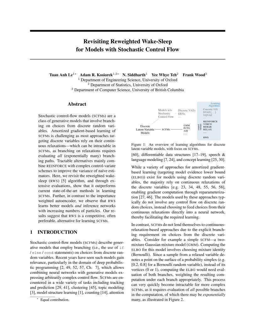
Figure 1: An overview of learning algorithms for discretelatent-variable models, with focus on SCFMs.

[60], differentiable data structures [17–19], speech &language modeling [7, 24], and concept learning [25, 30].

While a variety of approaches for amortized gradient-based learning (targeting model evidence lower bound(ELBO)) exist for models using discrete random vari-ables, the majority rely on continuous relaxations ofthe discrete variables [e.g. 23, 34, 48, 55, 56, 58],enabling gradient computation through reparameteriza-tion [27, 46]. The models used by these approaches typ-ically do not involve any control flow on discrete ran-dom choices, instead choosing to feed choices from theircontinuous relaxations directly into a neural network,thereby facilitating the required learning.

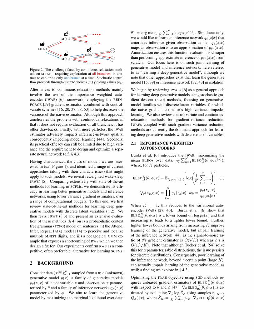
In contrast, SCFMs do not lend themselves to continuous-relaxation-based approaches due to the explicit branch-ing requirement on choices from the discrete vari-ables. Consider for example a simple SCFM—a two-mixture Gaussian mixture model (GMM). Computing theELBO for this model involves choosing mixture identity(Bernoulli). Since a sample from a relaxed variable de-notes a point on the surface of a probability simplex (e.g.[0.2, 0.8] for a Bernoulli random variable), instead of itsvertices (0 or 1), computing the ELBO would need eval-uation of both branches, weighting the resulting com-putation under each branch appropriately. This processcan very quickly become intractable for more complexSCFMs, as it requires evaluation of all possible branchesin the computation, of which there may be exponentiallymany, as illustrated in Figure 2.

if(c1)

if(c2)

. . .

. . .

if(c3)

if(c4)

v1

v2

. . .

Figure 2: The challenge faced by continuous-relaxation meth-ods on SCFMs—requiring exploration of all branches, in con-trast to exploring only one branch at a time. Stochastic controlflow proceeds through discrete choices (ci) yielding values (vi).

Alternatives to continuous-relaxation methods mainlyinvolve the use of the importance weighted auto-encoder (IWAE) [6] framework, employing the REIN-FORCE [59] gradient estimator, combined with control-variate schemes [16, 20, 37, 38, 53] to help decrease thevariance of the naıve estimator. Although this approachameliorates the problem with continuous relaxations inthat it does not require evaluation of all branches, it hasother drawbacks. Firstly, with more particles, the IWAEestimator adversely impacts inference-network quality,consequently impeding model learning [44]. Secondly,its practical efficacy can still be limited due to high vari-ance and the requirement to design and optimize a sepa-rate neural network (c.f. § 4.3).

Having characterized the class of models we are inter-ested in (c.f. Figure 1), and identified a range of currentapproaches (along with their characteristics) that mightapply to such models, we revisit reweighted wake-sleep(RWS) [5]. Comparing extensively with state-of-the-artmethods for learning in SCFMs, we demonstrate its effi-cacy in learning better generative models and inferencenetworks, using lower variance gradient estimators, overa range of computational budgets. To this end, we firstreview state-of-the-art methods for learning deep gen-erative models with discrete latent variables (§ 2). Wethen revisit RWS (§ 3) and present an extensive evalua-tion of these methods (§ 4) on i) a probabilistic contextfree grammar (PCFG) model on sentences, ii) the Attend,Infer, Repeat (AIR) model [14] to perceive and localizemultiple MNIST digits, and iii) a pedagogical GMM ex-ample that exposes a shortcoming of RWS which we thendesign a fix for. Our experiments confirm RWS as a com-petitive, often preferable, alternative for learning SCFMs.

2 BACKGROUND

Consider data (x(n))Nn=1 sampled from a true (unknown)generative model p(x), a family of generative modelspθ(z, x) of latent variable z and observation x parame-terized by θ and a family of inference networks qφ(z|x)parameterized by φ. We aim to learn the generativemodel by maximizing the marginal likelihood over data:

θ∗ = arg maxθ1N

∑Nn=1 log pθ(x

(n)). Simultaneously,we would like to learn an inference network qφ(z|x) thatamortizes inference given observation x; i.e., qφ(z|x)maps an observation x to an approximation of pθ∗(z|x).Amortization ensures this function evaluation is cheaperthan performing approximate inference of pθ∗(z|x) fromscratch. Our focus here is on such joint learning ofgenerative model and inference network, here referredto as “learning a deep generative model”, although wenote that other approaches exist that learn the generativemodel [15, 39] or inference network [32, 43] in isolation.

We begin by reviewing IWAEs [6] as a general approachfor learning deep generative models using stochastic gra-dient descent (SGD) methods, focusing on generative-model families with discrete latent variables, for whichthe naıve gradient estimator’s high variance impedeslearning. We also review control-variate and continuous-relaxation methods for gradient-variance reduction.IWAEs coupled with such gradient-variance reductionmethods are currently the dominant approach for learn-ing deep generative models with discrete latent variables.

2.1 IMPORTANCE WEIGHTEDAUTOENCODERS

Burda et al. [6] introduce the IWAE, maximizing themean ELBOs over data, 1

N

∑Nn=1 ELBOKIS (θ, φ, x(n)),

where, for K particles,

ELBOKIS (θ, φ, x) = EQφ(z1:K |x)

[log

(1

K

K∑k=1

wk

)], (1)

Qφ(z1:K |x) =

K∏k=1

qφ(zk|x), wk =pθ(zk, x)

qφ(zk|x).

When K = 1, this reduces to the variational auto-encoder (VAE) [27, 46]. Burda et al. [6] show thatELBOKIS (θ, φ, x) is a lower bound on log pθ(x) and thatincreasing K leads to a tighter lower bound. Further,tighter lower bounds arising from increasing K improvelearning of the generative model, but impair learningof the inference network [44], as the signal-to-noise ra-tio of θ’s gradient estimator is O(

√K) whereas φ’s is

O(1/√K). Note that although Tucker et al. [54] solve

this for reparameterizable distributions, the issue persistsfor discrete distributions. Consequently, poor learning ofthe inference network, beyond a certain point (large K),can actually impair learning of the generative model aswell; a finding we explore in § 4.3.

Optimizing the IWAE objective using SGD methods re-quires unbiased gradient estimators of ELBOKIS (θ, φ, x)with respect to θ and φ [47]. ∇θ ELBOKIS (θ, φ, x) is es-timated by evaluating ∇θ log ZK using samples z1:K ∼Qφ(·|x), where ZK = 1

K

∑Kk=1wk. ∇φELBOKIS(θ, φ, x)

is estimated similarly for models with reparameterizablelatents, discrete (and other non-reparameterizable) la-tents require the REINFORCE gradient estimator [59]

gREINFORCE =log ZK∇φ logQφ(z1:K |x)︸ ︷︷ ︸1

+∇φ log ZK︸ ︷︷ ︸2

. (2)

2.2 CONTINUOUS RELAXATIONS ANDCONTROL VARIATES

Since the gradient estimator in (2) typically suffers fromhigh variance, mainly due to the effect of 1 , a number ofapproaches have been developed to ameliorate the issue.These can be broadly categorized into approaches thatdirectly transform the discrete latent variables (continu-ous relaxations), or approaches that target improvementof the naıve REINFORCE estimator (control variates).

Continuous Relaxations: Here, discrete variables aretransformed to enable reparameterization [27, 46], help-ing reduce gradient-estimator variance. Approaches spanthe Gumbel distribution [23, 34], spike-and-X trans-forms [48], overlapping exponentials [56], and general-ized overlapping exponentials for tighter bounds [55].

Besides difficulties inherent to such methods, such astuning temperature parameters, or the suitability of undi-rected Boltzmann machine priors, these methods arenot well suited for learning SCFMs as they generatesamples on the surface of a probability simplex ratherthan its vertices. For example, sampling from a trans-formed Bernoulli distribution yields samples of the form[α, (1 − α)] rather than simply 0 or 1—the latter formrequired for branching. With relaxed samples, as illus-trated in Figure 2, one would need to execute all the ex-ponentially many discrete-variable driven branches in themodel, weighting each branch appropriately—somethingthat can quickly become infeasible for even moderatelycomplex models. However, for purposes of comparison,for relatively simple SCFMs, one could apply methods in-volving continuous relaxations, as demonstrated in § 4.3.

Control Variates: Here, approaches build on the RE-INFORCE estimator for the IWAE ELBO objective, de-signing control-variate schemes to reduce the varianceof the naıve estimator. Variational inference for MonteCarlo objectives (VIMCO) [38] eschews designing an ex-plicit control variate, instead exploiting the particle setobtained in IWAE. It replaces 1 with

g1

VIMCO =

K∑k=1

(log ZK −Υ−k)∇φ log qφ(zk|x), (3)

Υ−k = log1

K

(exp

(1

K − 1

∑6=k

logw`

)+∑6=k

w`

)

where Υ−k ⊥⊥ zk and highly correlated with log ZK .

Finally, assuming zk is a discrete random variable withC categories1, REBAR [53] and RELAX [16] improve onMnih and Gregor [37] and Gu et al. [20], replacing 1 as

g1

RELAX =

(log ZK − cρ(g1:K)

)∇φ logQφ(z1:K |x)

+∇φcρ(g1:K)−∇φcρ(g1:K), (4)

where gk is a C-dimensional vector of reparameterizedGumbel random variates, zk is a one-hot argmax func-tion of gk, and gk is a vector of reparameterized condi-tional Gumbel random variates conditioned on zk. Theconditional Gumbel random variates are a form of Rao-Blackwellization used to reduce variance. The controlvariate cρ, parameterized by ρ, is optimized to mini-mize the gradient variance estimates along with the mainELBO optimization, leading to state-of-the-art perfor-mance on, for example, sigmoid belief networks [40].The main difficulty in using this method is choosing asuitable family of cρ, as some choices lead to higher vari-ance despite concurrent gradient-variance minimization.

3 REVISITING REWEIGHTEDWAKE-SLEEP

Reweighted wake-sleep (RWS) [5] comes from a familyof algorithms [11, 22] for learning deep generative mod-els, eschewing a single objective over parameters θ and φin favour of individual objectives for each. We review theRWS algorithm and discuss its pros and cons.

3.1 REWEIGHTED WAKE-SLEEP

Reweighted wake-sleep (RWS) [5] is an extension of thewake-sleep algorithm [11, 22] both of which, like IWAE,jointly learn a generative model and an inference net-work given data. While IWAE targets a single objective,RWS alternates between objectives, updating the genera-tive model parameters θ using a wake-phase θ update andthe inference network parameters φ using either a sleep-or a wake-phase φ update (or both).

Wake-phase θ update. Given φ, θ is updated using anunbiased estimate of∇θ−

(1N

∑Nn=1ELBOKIS (θ, φ, x(n))

),

obtained without reparameterization or control variates,as the sampling distributionQφ(·|x) is independent of θ.2

1The assumption is needed only for notational convenience.However, using more structured latents leads to difficulties inpicking the control-variate architecture.

2We assume that the deterministic mappings induced by theparameters θ, φ are themselves differentiable, such that they areamenable to gradient-based learning.

Sleep-phase φ update. Here, φ is updated to minimizethe Kullback-Leibler (KL) divergence between the poste-riors under the generative model and the inference net-work, averaged over the data distribution of the currentgenerative model

Epθ(x)[DKL(pθ(z|x), qφ(z|x))]

= Epθ(z,x)[log pθ(z|x)− log qφ(z|x)]. (5)

Its gradient, Epθ(z,x)[−∇φ log qφ(z|x)], is estimated byevaluating−∇φ log qφ(z|x), where z, x ∼ pθ(z, x). Theestimator’s variance can be reduced at a standard MonteCarlo rate by increasing the number of samples of z, x.

Wake-phase φ update. Here, φ is updated to minimizethe KL divergence between the posteriors under the gen-erative model and the inference network, averaged overthe true data distribution

Ep(x)[DKL(pθ(z|x), qφ(z|x))]

= Ep(x)[Epθ(z|x)[log pθ(z|x)− log qφ(z|x)]]. (6)

The outer expectation Ep(x)[Epθ(z|x)[−∇φ log qφ(z|x)]]of the gradient is estimated using a single sample x fromthe true data distribution p(x), given which, the inner ex-pectation is estimated using self-normalized importancesampling withK particles, using qφ(z|x) as the proposaldistribution. This results in the following estimator

K∑k=1

wk∑K`=1 w`

(−∇φ log qφ(zk|x)) , (7)

where, similar to (1), x ∼ p(x), zk ∼ qφ(zk|x), andwk = pθ(zk, x)/qφ(zk|x). Note that (7) is the nega-tive of the second term of the REINFORCE estimator ofthe IWAE ELBO in (2). The crucial difference betweenthe wake-phase φ update and the sleep-phase φ updateis that the expectation in (6) is over the true data distri-bution p(x) and the expectation in (5) is under the cur-rent model distribution pθ(x). The former is desirablefrom the perspective of amortizing inference over datafrom p(x), and although its estimator is biased, this biasdecreases as K increases.

3.2 PROS OF REWEIGHTED WAKE-SLEEP

While the gradient update of θ targets the same objectiveas IWAE, the gradient update of φ targets the objective in(5) in the sleep case and (6) in the wake case. This makesRWS a preferable option to IWAE for learning inferencenetworks because the φ updates in RWS directly targetminimization of the expected KL divergences from thetrue to approximate posterior. With an increased com-putational budget, using more Monte Carlo samples inthe sleep-phase φ update case and more particles K in

the wake-phase φ update, we obtain a better estimatorof these expected KL divergences. This is in contrast toIWAE, where optimizing ELBOKIS targets a KL divergenceon an extended sampling space [33] which for K > 1doesn’t correspond to a KL divergence between true andapproximate posteriors (in any order). Consequently, in-creasing K in IWAE leads to impaired learning of infer-ence networks [44].

Moreover, targeting DKL(p, q) as in RWS can be prefer-able to targeting DKL(q, p) as in VAEs. The former en-courages mean-seeking behavior, having the inferencenetwork to put non-zero mass in regions where the pos-terior has non-zero mass, whereas the latter encouragesmode-seeking behavior, having the inference network toput mass on one of the modes of the posterior [36]. Us-ing the inference network as an importance sampling (IS)proposal requires mean-seeking behavior [42, Theorem9.2]. Moreover, Chatterjee et al. [8] show that the num-ber of particles required for IS to accurately approximateexpectations of the form Ep(z|x)[f(z)] is directly relatedto exp(DKL(p, q)).

3.3 CONS OF REWEIGHTED WAKE-SLEEP

While a common criticism of the wake-sleep family ofalgorithms is the lack of a unifying objective, we havenot found any empirical evidence where this is a prob-lem. Perhaps a more relevant criticism is that both thesleep and wake-phase φ gradient estimators are biasedwith respect to ∇φEp(x)[DKL(pθ(z|x), qφ(z|x))]. Thebias in the sleep-phase φ gradient estimator arises fromtargeting the expectation under the model rather than thetrue data distribution, and the bias in the wake-phase φgradient estimator results from estimating the KL diver-gence using self-normalized IS.

In theory, these biases should not affect the fixed pointof optimization (θ∗, φ∗) where pθ∗(x) = p(x) andqφ∗(z|x) = pθ∗(z|x). First, if θ → θ∗ through the wake-phase θ update, the data distribution bias reduces to zero.Second, although the wake-phase φ gradient estimator isbiased, it is consistent—with large enough K, conver-gence of stochastic optimization is theoretically guaran-teed on convex objectives and empirically on non-convexobjectives [10]. Further, this gradient estimator followsthe central limit theorem, so its asymptotic variance de-creases linearly with K [42, Eq. (9.8)]. Thus, usinglarger K improves learning of the inference network.

In practice, the families of generative models, inferencenetworks, and the data distributions determine which ofthe biases are more significant. In most of our findings,the bias of the data distribution appears to be the mostdetrimental. This is due to the fact that initially pθ(x) isquite different from p(x), and hence using sleep-phase

φ updates performs worse than using wake-phase φ up-dates. An exception to this is the PCFG experiment (c.f.§ 4.1) where the data distribution bias is not as large andinference using self-normalized IS is extremely difficult.

4 EXPERIMENTS

The IWAE and RWS algorithms have primarily beenapplied to problems with continuous latent variablesand/or discrete latent variables that do not actually in-duce branching (such as sigmoid belief networks; [40]).The purpose of the following experiments is to compareRWS to IWAE combined with control variates and con-tinuous relaxations (c.f § 3) on models with conditionalbranching, and show that it outperform such methods.We empirically demonstrate that increasing the numberof particles K can be detrimental in IWAE but advanta-geous in RWS, as evidenced by achieved ELBOs and av-erage distance between true and amortized posteriors.

In the first experiment, we present learning and amor-tized inference in a PCFG [4], an example SCFM wherecontinuous relaxations are inapplicable. We demonstratethat RWS outperforms IWAE with a control variate both interms of learning and inference. The second experimentfocuses on Attend, Infer, Repeat (AIR), the deep gener-ative model of [14]. It demonstrates that RWS leads tobetter learning of the generative model in a setting withboth discrete and continuous latent variables, for model-ing a complex visual data domain (c.f. § 4.2). The finalexperiment involves a GMM (§ 4.3), thereby serving as apedagogical example. It explains the causes of why RWSmight be preferable to other methods in more detail. 3

Notationally, the different variants of RWS will be re-ferred to as wake-sleep (WS) and wake-wake (WW). Thewake-phase θ update is always used. We refer to using itin conjunction with the sleep-phase φ update as WS andusing it in conjunction with the wake-phase φ update asWW. Using both wake- and sleep-phase φ updates dou-bles the required stochastic sampling while yielding onlyminor improvements on the models we considered. Thenumber of particles K used for the wake-phase θ andφ updates is always specified, and computation betweenthem is matched so a wake-phase φ update with batchsizeB implies a sleep phase φ update withKB samples.

4.1 PROBABILISTIC CONTEXT-FREEGRAMMAR

In this experiment we learn model parameters and amor-tize inference in a PCFG [4]. Each discrete latent variablein a PCFG chooses a particular child of a node in a tree.

3In Appendix D, we include additional experiments on sig-moid belief networks which, however, are not SCFMs.

Depending on each discrete choice, the generative modelcan lead to different future latent variables. A PCFG is anexample of an SCFM where continuous relaxations can-not be applied—weighing combinatorially many futuresby a continuous relaxation is infeasible and doing so forfutures which have infinite latent variables is impossible.

While supervised approaches have recently led to state-of-the-art performance in parsing [9], PCFGs remainone of the key models for unsupervised parsing [35].Learning in a PCFG is typically done via expectation-maximization [12] which uses the inside-outside algo-rithm [31]. Inference methods are based on dynamicprogramming [13, 61] or search [28]. Applying RWS andIWAE algorithms to PCFGs allows learning from large un-labeled datasets through SGD while inference amortiza-tion ensures linear-time parsing in the number of wordsin a sentence, at test-time. Moreover, using the inferencenetwork as a proposal distribution in IS provides asymp-totically exact posteriors if parses are ambiguous.

A PCFG is defined by sets of terminals (or words) {ti},non-terminals {ni}, production rules {ni → ζj} with ζja sequence of terminals and non-terminals, probabilitiesfor each production rule such that

∑j P (ni→ζj) = 1

for each ni, and a start symbol n1. Consider the As-tronomers PCFG given in Manning et al. [35, Table 11.2](c.f. Appendix A). A parse tree z is obtained by recur-sively applying the production rules until there are nomore non-terminals. For example, a parse tree (S (NPastronomers) (VP (V saw) (NP stars))) is obtained by ap-plying the production rules as follows:

S 1.0−−→ NP VP 0.1−−→ astronomers VP 0.7−−→ astronomers V NP1.0−−→ astronomers saw NP 0.18−−→ astronomers saw stars,

where the probability p(z) is obtained by multiplying thecorresponding production probabilities as indicated ontop of the arrows. The likelihood of a PCFG, p(x|z), is1 if the sentence x matches the sentence produced by z(in this case “astronomers saw stars”) and 0 otherwise.One can easily construct infinitely long z by choosingproductions which contain non-terminals, for example:S→ NP VP→ NP PP VP→ NP PP PP VP→ · · · .We learn the production probabilities of the PCFG and aninference network computing the conditional distributionof a parse tree given a sentence. The architecture of theinference network is the same as described in [32, Sec-tion 3.3] except the input to the recurrent neural network(RNN) consists only of the sentence embedding, previ-ous sample embedding, and an address embedding. Eachword is represented as a one-hot vector and the sentenceembedding is obtained through another RNN. Instead ofa hard {0, 1} likelihood which can make learning diffi-cult, we use a relaxation, p(x|z) = exp(−L(x, s(z))2),

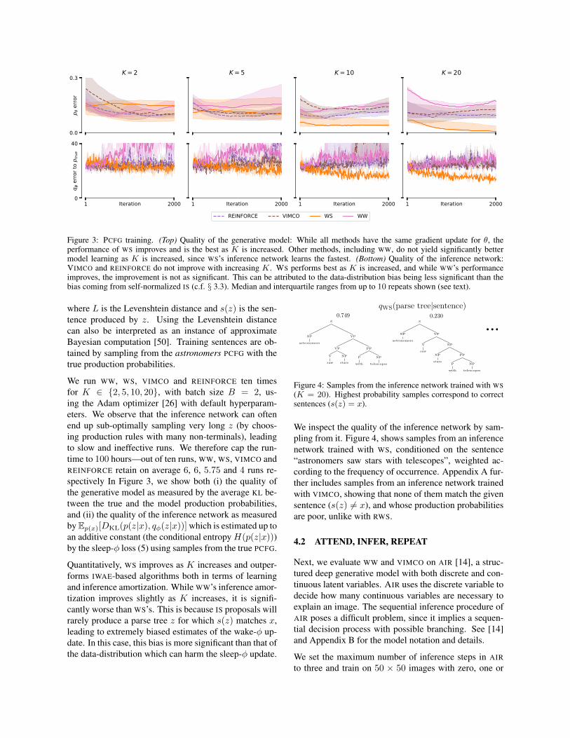
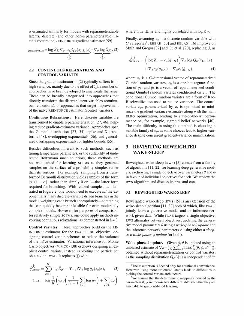
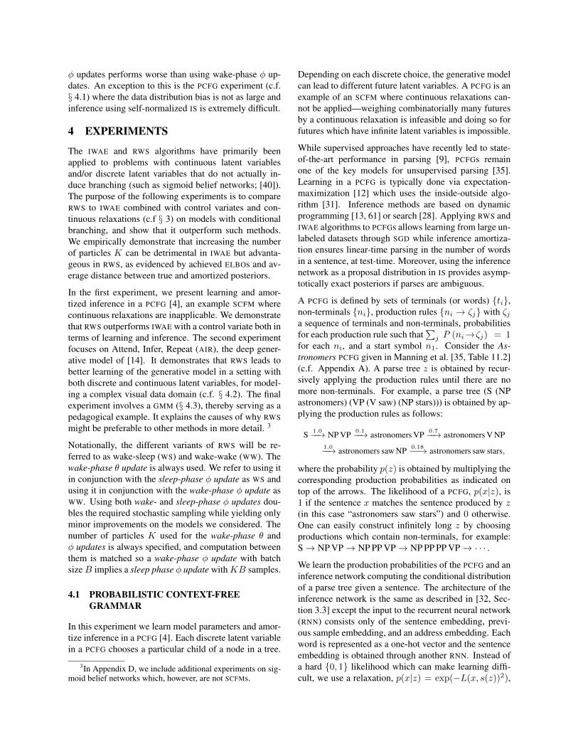
Figure 3: PCFG training. (Top) Quality of the generative model: While all methods have the same gradient update for θ, theperformance of WS improves and is the best as K is increased. Other methods, including WW, do not yield significantly bettermodel learning as K is increased, since WS’s inference network learns the fastest. (Bottom) Quality of the inference network:VIMCO and REINFORCE do not improve with increasing K. WS performs best as K is increased, and while WW’s performanceimproves, the improvement is not as significant. This can be attributed to the data-distribution bias being less significant than thebias coming from self-normalized IS (c.f. § 3.3). Median and interquartile ranges from up to 10 repeats shown (see text).

where L is the Levenshtein distance and s(z) is the sen-tence produced by z. Using the Levenshtein distancecan also be interpreted as an instance of approximateBayesian computation [50]. Training sentences are ob-tained by sampling from the astronomers PCFG with thetrue production probabilities.

We run WW, WS, VIMCO and REINFORCE ten timesfor K ∈ {2, 5, 10, 20}, with batch size B = 2, us-ing the Adam optimizer [26] with default hyperparam-eters. We observe that the inference network can oftenend up sub-optimally sampling very long z (by choos-ing production rules with many non-terminals), leadingto slow and ineffective runs. We therefore cap the run-time to 100 hours—out of ten runs, WW, WS, VIMCO andREINFORCE retain on average 6, 6, 5.75 and 4 runs re-spectively In Figure 3, we show both (i) the quality ofthe generative model as measured by the average KL be-tween the true and the model production probabilities,and (ii) the quality of the inference network as measuredby Ep(x)[DKL(p(z|x), qφ(z|x))] which is estimated up toan additive constant (the conditional entropy H(p(z|x)))by the sleep-φ loss (5) using samples from the true PCFG.

Quantitatively, WS improves as K increases and outper-forms IWAE-based algorithms both in terms of learningand inference amortization. While WW’s inference amor-tization improves slightly as K increases, it is signifi-cantly worse than WS’s. This is because IS proposals willrarely produce a parse tree z for which s(z) matches x,leading to extremely biased estimates of the wake-φ up-date. In this case, this bias is more significant than that ofthe data-distribution which can harm the sleep-φ update.

S

NP

astronomers

VP

VP

V

saw

NP

stars

PP

P

with

NP

telescopes

S

NP

astronomers

VP

V

saw

NP

NP

stars

PP

P

with

NP

telescopes

0:749 0:230

qWS(parse treejsentence)

Figure 4: Samples from the inference network trained with WS(K = 20). Highest probability samples correspond to correctsentences (s(z) = x).

We inspect the quality of the inference network by sam-pling from it. Figure 4, shows samples from an inferencenetwork trained with WS, conditioned on the sentence“astronomers saw stars with telescopes”, weighted ac-cording to the frequency of occurrence. Appendix A fur-ther includes samples from an inference network trainedwith VIMCO, showing that none of them match the givensentence (s(z) 6= x), and whose production probabilitiesare poor, unlike with RWS.

4.2 ATTEND, INFER, REPEAT

Next, we evaluate WW and VIMCO on AIR [14], a struc-tured deep generative model with both discrete and con-tinuous latent variables. AIR uses the discrete variable todecide how many continuous variables are necessary toexplain an image. The sequential inference procedure ofAIR poses a difficult problem, since it implies a sequen-tial decision process with possible branching. See [14]and Appendix B for the model notation and details.

We set the maximum number of inference steps in AIRto three and train on 50 × 50 images with zero, one or

0 200 400 600 800 1000

epoch

−120

−115

−110

−105

−100

log

pθ(x

)

IWAE+VIMCO K=80

IWAE+VIMCO K=40

IWAE+VIMCO K=20

IWAE+VIMCO K=10

IWAE+VIMCO K=5

WW K=80

WW K=40

WW K=20

WW K=10

WW K=5

5 10 20 40 80

number of particles

−106

−104

−102

−100

−98

log

pθ(x

)

IWAE+VIMCO

WW

0 200 400 600 800 1000

epoch

6

8

10

12

14

16

18

20

KL

(qφ

(z|x

)||

pθ(z|x

))

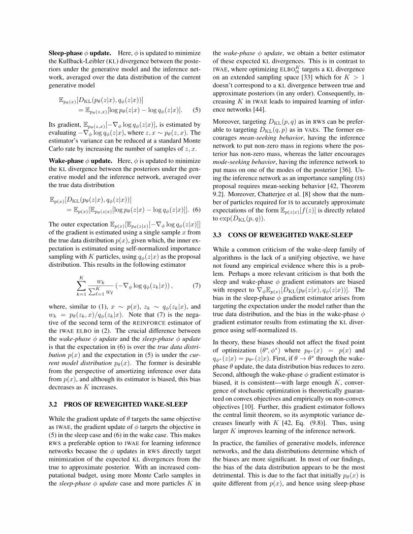
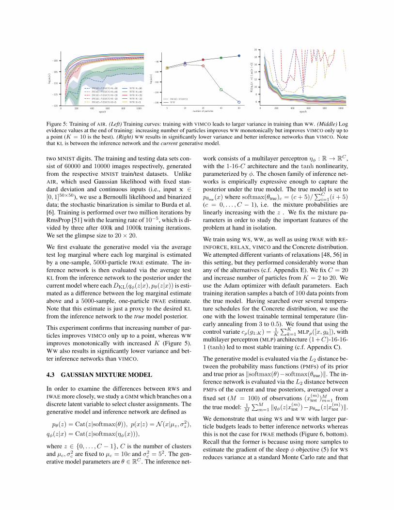
Figure 5: Training of AIR. (Left) Training curves: training with VIMCO leads to larger variance in training than WW. (Middle) Logevidence values at the end of training: increasing number of particles improves WW monotonically but improves VIMCO only up toa point (K = 10 is the best). (Right) WW results in significantly lower variance and better inference networks than VIMCO. Notethat KL is between the inference network and the current generative model.

two MNIST digits. The training and testing data sets con-sist of 60000 and 10000 images respectively, generatedfrom the respective MNIST train/test datasets. UnlikeAIR, which used Gaussian likelihood with fixed stan-dard deviation and continuous inputs (i.e., input x ∈[0, 1]50×50), we use a Bernoulli likelihood and binarizeddata; the stochastic binarization is similar to Burda et al.[6]. Training is performed over two million iterations byRmsProp [51] with the learning rate of 10−5, which is di-vided by three after 400k and 1000k training iterations.We set the glimpse size to 20× 20.

We first evaluate the generative model via the averagetest log marginal where each log marginal is estimatedby a one-sample, 5000-particle IWAE estimate. The in-ference network is then evaluated via the average testKL from the inference network to the posterior under thecurrent model where eachDKL(qφ(z|x), pθ(z|x)) is esti-mated as a difference between the log marginal estimateabove and a 5000-sample, one-particle IWAE estimate.Note that this estimate is just a proxy to the desired KLfrom the inference network to the true model posterior.

This experiment confirms that increasing number of par-ticles improves VIMCO only up to a point, whereas WWimproves monotonically with increased K (Figure 5).WW also results in significantly lower variance and bet-ter inference networks than VIMCO.

4.3 GAUSSIAN MIXTURE MODEL

In order to examine the differences between RWS andIWAE more closely, we study a GMM which branches on adiscrete latent variable to select cluster assignments. Thegenerative model and inference network are defined as

pθ(z) = Cat(z|softmax(θ)), p(x|z) = N (x|µz, σ2z),

qφ(z|x) = Cat(z|softmax(ηφ(x))),

where z ∈ {0, . . . , C − 1}, C is the number of clustersand µc, σ2

c are fixed to µc = 10c and σ2c = 52. The gen-

erative model parameters are θ ∈ RC . The inference net-

work consists of a multilayer perceptron ηφ : R → RC ,with the 1-16-C architecture and the tanh nonlinearity,parameterized by φ. The chosen family of inference net-works is empirically expressive enough to capture theposterior under the true model. The true model is set topθtrue(x) where softmax(θtrue)c = (c+ 5)/

∑Ci=1(i+ 5)

(c = 0, . . . , C − 1), i.e. the mixture probabilities arelinearly increasing with the z . We fix the mixture pa-rameters in order to study the important features of theproblem at hand in isolation.

We train using WS, WW, as well as using IWAE with RE-INFORCE, RELAX, VIMCO and the Concrete distribution.We attempted different variants of relaxations [48, 56] inthis setting, but they performed considerably worse thanany of the alternatives (c.f. Appendix E). We fix C = 20and increase number of particles from K = 2 to 20. Weuse the Adam optimizer with default parameters. Eachtraining iteration samples a batch of 100 data points fromthe true model. Having searched over several tempera-ture schedules for the Concrete distribution, we use theone with the lowest trainable terminal temperature (lin-early annealing from 3 to 0.5). We found that using thecontrol variate cρ(g1:K) = 1

K

∑Kk=1 MLPρ([x, gk]), with

multilayer perceptron (MLP) architecture (1+C)-16-16-1 (tanh) led to most stable training (c.f. Appendix C).

The generative model is evaluated via theL2 distance be-tween the probability mass functions (PMFs) of its priorand true prior as ‖softmax(θ)−softmax(θtrue)‖. The in-ference network is evaluated via the L2 distance betweenPMFs of the current and true posteriors, averaged over afixed set (M = 100) of observations (x

(m)test )Mm=1 from

the true model: 1M

∑Mm=1 ‖qφ(z|x(m)

test )−pθtrue(z|x(m)test )‖.

We demonstrate that using WS and WW with larger par-ticle budgets leads to better inference networks whereasthis is not the case for IWAE methods (Figure 6, bottom).Recall that the former is because using more samples toestimate the gradient of the sleep φ objective (5) for WSreduces variance at a standard Monte Carlo rate and that

10−2

10−1

100‖pθ

(z)−

pθ

tru

e(z

)‖K = 2 K = 5 K = 10 K = 20

1 100000Iteration

10−1

100

Avg

.te

st‖qφ

(z|x

)−

pθ

tru

e(z|x

)‖

1 100000Iteration

Concrete RELAX REINFORCE VIMCO WS WW δ-WW

1 100000Iteration 1 100000Iteration

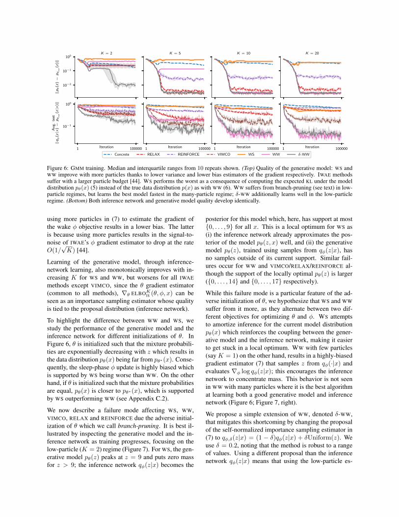
Figure 6: GMM training. Median and interquartile ranges from 10 repeats shown. (Top) Quality of the generative model: WS andWW improve with more particles thanks to lower variance and lower bias estimators of the gradient respectively. IWAE methodssuffer with a larger particle budget [44]. WS performs the worst as a consequence of computing the expected KL under the modeldistribution pθ(x) (5) instead of the true data distribution p(x) as with WW (6). WW suffers from branch-pruning (see text) in low-particle regimes, but learns the best model fastest in the many-particle regime; δ-WW additionally learns well in the low-particleregime. (Bottom) Both inference network and generative model quality develop identically.

using more particles in (7) to estimate the gradient ofthe wake φ objective results in a lower bias. The latteris because using more particles results in the signal-to-noise of IWAE’s φ gradient estimator to drop at the rateO(1/

√K) [44].

Learning of the generative model, through inference-network learning, also monotonically improves with in-creasing K for WS and WW, but worsens for all IWAEmethods except VIMCO, since the θ gradient estimator(common to all methods), ∇θ ELBOKIS (θ, φ, x) can beseen as an importance sampling estimator whose qualityis tied to the proposal distribution (inference network).

To highlight the difference between WW and WS, westudy the performance of the generative model and theinference network for different initializations of θ. InFigure 6, θ is initialized such that the mixture probabili-ties are exponentially decreasing with z which results inthe data distribution pθ(x) being far from pθ∗(x). Conse-quently, the sleep-phase φ update is highly biased whichis supported by WS being worse than WW. On the otherhand, if θ is initialized such that the mixture probabilitiesare equal, pθ(x) is closer to pθ∗(x), which is supportedby WS outperforming WW (see Appendix C.2).

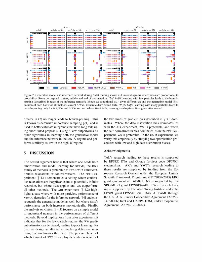
We now describe a failure mode affecting WS, WW,VIMCO, RELAX and REINFORCE due the adverse initial-ization of θ which we call branch-pruning. It is best il-lustrated by inspecting the generative model and the in-ference network as training progresses, focusing on thelow-particle (K = 2) regime (Figure 7). For WS, the gen-erative model pθ(z) peaks at z = 9 and puts zero massfor z > 9; the inference network qφ(z|x) becomes the

posterior for this model which, here, has support at most{0, . . . , 9} for all x. This is a local optimum for WS as(i) the inference network already approximates the pos-terior of the model pθ(z, x) well, and (ii) the generativemodel pθ(z), trained using samples from qφ(z|x), hasno samples outside of its current support. Similar fail-ures occur for WW and VIMCO/RELAX/REINFORCE al-though the support of the locally optimal pθ(z) is larger({0, . . . , 14} and {0, . . . , 17} respectively).

While this failure mode is a particular feature of the ad-verse initialization of θ, we hypothesize that WS and WWsuffer from it more, as they alternate between two dif-ferent objectives for optimizing θ and φ. WS attemptsto amortize inference for the current model distributionpθ(x) which reinforces the coupling between the gener-ative model and the inference network, making it easierto get stuck in a local optimum. WW with few particles(say K = 1) on the other hand, results in a highly-biasedgradient estimator (7) that samples z from qφ(·|x) andevaluates ∇φ log qφ(z|x); this encourages the inferencenetwork to concentrate mass. This behavior is not seenin WW with many particles where it is the best algorithmat learning both a good generative model and inferencenetwork (Figure 6; Figure 7, right).

We propose a simple extension of WW, denoted δ-WW,that mitigates this shortcoming by changing the proposalof the self-normalized importance sampling estimator in(7) to qφ,δ(z|x) = (1 − δ)qφ(z|x) + δUniform(z). Weuse δ = 0.2, noting that the method is robust to a rangeof values. Using a different proposal than the inferencenetwork qφ(z|x) means that using the low-particle es-

Iter

.0

pθ(z) qφ(z|x = 0)

K = 2

qφ(z|x = 95) qφ(z|x = 190) pθ(z) qφ(z|x = 0)

K = 20

qφ(z|x = 95) qφ(z|x = 190)

Iter

.4

90

00

z

Iter

.9

90

00

z z z z

True Concrete RELAX REINFORCE VIMCO WS WW δ-WW

z z z

Figure 7: Generative model and inference network during GMM training shown as Hinton diagrams where areas are proportional toprobability. Rows correspond to start, middle and end of optimization. (Left half) Learning with few particles leads to the branch-pruning (described in text) of the inference network (shown as conditional PMF given different x) and the generative model (firstcolumn of each half) for all methods except δ-WW. Concrete distribution fails. (Right half) Learning with many particles leads tobranch-pruning only for WS; WW and δ-WW succeed where IWAE fails, learning a suboptimal final generative model.

timator in (7) no longer leads to branch-pruning. Thisis known as defensive importance sampling [21], and isused to better estimate integrands that have long tails us-ing short-tailed proposals. Using δ-WW outperforms allother algorithms in learning both the generative modeland the inference network in the low-K regime and per-forms similarly as WW in the high-K regime.

5 DISCUSSION

The central argument here is that where one needs bothamortization and model learning for SCFMs, the RWSfamily of methods is preferable to IWAE with either con-tinuous relaxations or control-variates. The PCFG ex-periment (§ 4.1) demonstrates a setting where continu-ous relaxations are inapplicable due to potentially infiniterecursion, but where RWS applies and WS outperformsall other methods. The AIR experiment (§ 4.2) high-lights a case where with more particles, performance ofVIMCO degrades for the inference network [44] and con-sequently the generative model as well, but where RWS’sperformance on both increases monotonically. Finally,the analysis on GMMs (§ 4.3) focuses on a simple modelto understand nuances in the performances of differentmethods. Beyond implications from prior experiments, itindicates that for the few-particle regime, the WW gradi-ent estimator can be biased, leading to poor learning. Forthis, we design an alternative involving defensive sam-pling that ameliorates the issue. The precise choice ofwhich variant of RWS to employ depends on which of

the two kinds of gradient bias described in § 3.3 dom-inates. Where the data distribution bias dominates, aswith the AIR experiment, WW is preferable, and wherethe self-normalized IS bias dominates, as in the PCFG ex-periment, WS is preferable. In the GMM experiment, weverify this empirically by studying two optimization pro-cedures with low and high data distribution biases.

Acknowledgments

TAL’s research leading to these results is supportedby EPSRC DTA and Google (project code DF6700)studentships. AK’s and YWT’s research leading tothese results are supported by funding from the Eu-ropean Research Council under the European UnionsSeventh Framework Programme (FP7/2007-2013) ERCgrant agreement no. 617071. NS is supported by EP-SRC/MURI grant EP/N019474/1. FW’s research lead-ing is supported by The Alan Turing Institute under theEPSRC grant EP/N510129/1; DARPA PPAML throughthe U.S. AFRL under Cooperative Agreement FA8750-14-2-0006; Intel and DARPA D3M, under CooperativeAgreement FA8750-17-2-0093.

References

[1] Ryan Adams, Hanna Wallach, and Zoubin Ghahramani.Learning the structure of deep sparse graphical models.In International Conference on Artificial Intelligence andStatistics, 2010.

[2] Eli Bingham, Jonathan P Chen, Martin Jankowiak, FritzObermeyer, Neeraj Pradhan, Theofanis Karaletsos, RohitSingh, Paul Szerlip, Paul Horsfall, and Noah D Good-man. Pyro: Deep universal probabilistic programming.The Journal of Machine Learning Research, 20(1):973–978, 2019.

[3] David M Blei, Andrew Y Ng, and Michael I Jordan. La-tent dirichlet allocation. Journal of machine Learning re-search, 3(Jan):993–1022, 2003.

[4] Taylor L Booth and Richard A Thompson. Applyingprobability measures to abstract languages. IEEE trans-actions on Computers, 100(5):442–450, 1973.

[5] Jorg Bornschein and Yoshua Bengio. Reweighted wake-sleep. In International Conference on Learning Repre-sentations, 2015.

[6] Yuri Burda, Roger Grosse, and Ruslan Salakhutdinov.Importance weighted autoencoders. In International Con-ference on Learning Representations, 2016.

[7] Nick Chater and Christopher D Manning. Probabilisticmodels of language processing and acquisition. Trends incognitive sciences, 10(7):335–344, 2006.

[8] Sourav Chatterjee, Persi Diaconis, et al. The sample sizerequired in importance sampling. The Annals of AppliedProbability, 28(2):1099–1135, 2018.

[9] Danqi Chen and Christopher Manning. A fast and accu-rate dependency parser using neural networks. In Pro-ceedings of the 2014 conference on empirical methods innatural language processing (EMNLP), pages 740–750,2014.

[10] Jie Chen and Ronny Luss. Stochastic gradient descentwith biased but consistent gradient estimators. arXivpreprint arXiv:1807.11880, 2018.

[11] Peter Dayan, Geoffrey E Hinton, Radford M Neal, andRichard S Zemel. The Helmholtz machine. Neural com-putation, 7(5):889–904, 1995.

[12] Arthur P Dempster, Nan M Laird, and Donald B Rubin.Maximum likelihood from incomplete data via the em al-gorithm. Journal of the Royal Statistical Society: SeriesB (Methodological), 39(1):1–22, 1977.

[13] Jay Earley. An efficient context-free parsing algorithm.Communications of the ACM, 13(2):94–102, 1970.

[14] S. M. Ali Eslami, Nicolas Heess, Theophane Weber, Yu-val Tassa, David Szepesvari, Koray Kavukcuoglu, andGeoffrey E. Hinton. Attend, infer, repeat: Fast scene un-derstanding with generative models. In Advances in Neu-ral Information Processing Systems, 2016.

[15] Ian Goodfellow, Jean Pouget-Abadie, Mehdi Mirza, BingXu, David Warde-Farley, Sherjil Ozair, Aaron Courville,and Yoshua Bengio. Generative adversarial nets. In Ad-vances in neural information processing systems, pages2672–2680, 2014.

[16] Will Grathwohl, Dami Choi, Yuhuai Wu, Geoff Roeder,and David Duvenaud. Backpropagation through the void:Optimizing control variates for black-box gradient esti-mation. In International Conference on Learning Repre-sentations, 2018.

[17] Alex Graves, Greg Wayne, and Ivo Danihelka. NeuralTuring machines. arXiv preprint arXiv:1410.5401, 2014.

[18] Alex Graves, Greg Wayne, Malcolm Reynolds, TimHarley, Ivo Danihelka, Agnieszka Grabska-Barwinska,Sergio Gomez Colmenarejo, Edward Grefenstette, TiagoRamalho, John Agapiou, et al. Hybrid computing usinga neural network with dynamic external memory. Nature,538(7626):471, 2016.

[19] Edward Grefenstette, Karl Moritz Hermann, Mustafa Su-leyman, and Phil Blunsom. Learning to transduce withunbounded memory. In Advances in Neural InformationProcessing Systems, pages 1828–1836, 2015.

[20] Shixiang Gu, Sergey Levine, Ilya Sutskever, and AndriyMnih. Muprop: Unbiased backpropagation for stochasticneural networks. In International Conference on Learn-ing Representations, 2016.

[21] Tim Hesterberg. Weighted average importance samplingand defensive mixture distributions. Technometrics, 37(2):185–194, 1995.

[22] Geoffrey E Hinton, Peter Dayan, Brendan J Frey, andRadford M Neal. The “wake-sleep” algorithm for un-supervised neural networks. Science, 268(5214):1158–1161, 1995.

[23] Eric Jang, Shixiang Gu, and Ben Poole. Categorical repa-rameterization with Gumbel-softmax. In InternationalConference on Learning Representations, 2017.

[24] Biing Hwang Juang and Laurence R Rabiner. Hiddenmarkov models for speech recognition. Technometrics,33(3):251–272, 1991.

[25] Charles Kemp, Joshua B Tenenbaum, Thomas L Griffiths,Takeshi Yamada, and Naonori Ueda. Learning systems ofconcepts with an infinite relational model. 2006.

[26] Diederik P. Kingma and Jimmy Ba. Adam: A method forstochastic optimization. In International Conference onLearning Representations, 2015.

[27] Diederik P Kingma and Max Welling. Auto-encodingvariational Bayes. In International Conference on Learn-ing Representations, 2014.

[28] Dan Klein and Christopher D Manning. A parsing: fastexact viterbi parse selection. In Proceedings of the 2003Conference of the North American Chapter of the As-sociation for Computational Linguistics on Human Lan-guage Technology-Volume 1, pages 40–47. Associationfor Computational Linguistics, 2003.

[29] Adam R. Kosiorek, Hyunjik Kim, Ingmar Posner, andYee Whye Teh. Sequential attend, infer, repeat: Genera-tive modelling of moving objects. In Advances in NeuralInformation Processing Systems, 2018.

[30] Brenden M Lake, Neil D Lawrence, and Joshua B Tenen-baum. The emergence of organizing structure in concep-tual representation. Cognitive science, 2018.

[31] Karim Lari and Steve J Young. The estimation of stochas-tic context-free grammars using the inside-outside algo-rithm. Computer speech & language, 4(1):35–56, 1990.

[32] Tuan Anh Le, Atilim Gunes Baydin, and Frank Wood. In-ference compilation and universal probabilistic program-ming. In International Conference on Artificial Intelli-gence and Statistics, 2017.

[33] Tuan Anh Le, Maximilian Igl, Tom Rainforth, Tom Jin,and Frank Wood. Auto-encoding sequential Monte Carlo.In International Conference on Learning Representa-tions, 2018.

[34] Chris J Maddison, Andriy Mnih, and Yee Whye Teh. Theconcrete distribution: A continuous relaxation of discreterandom variables. In International Conference on Learn-ing Representations, 2017.

[35] Christopher D Manning, Christopher D Manning, andHinrich Schutze. Foundations of statistical natural lan-guage processing. MIT press, 1999.

[36] Tom Minka. Divergence measures and message passing.Technical report, Technical report, Microsoft Research,2005.

[37] Andriy Mnih and Karol Gregor. Neural variational in-ference and learning in belief networks. In Interna-tional Conference on Machine Learning, pages 1791–1799, 2014.

[38] Andriy Mnih and Danilo Rezende. Variational inferencefor Monte Carlo objectives. In International Conferenceon Machine Learning, pages 2188–2196, 2016.

[39] Shakir Mohamed and Balaji Lakshminarayanan. Learn-ing in implicit generative models. arXiv preprintarXiv:1610.03483, 2016.

[40] Radford M Neal. Connectionist learning of belief net-works. Artificial intelligence, 56(1):71–113, 1992.

[41] Willie Neiswanger, Frank Wood, and Eric Xing. Thedependent Dirichlet process mixture of objects fordetection-free tracking and object modeling. In ArtificialIntelligence and Statistics, pages 660–668, 2014.

[42] Art B. Owen. Monte Carlo theory, methods and exam-ples. 2013.

[43] Brooks Paige and Frank Wood. Inference networks forsequential monte carlo in graphical models. In Inter-national Conference on Machine Learning, pages 3040–3049, 2016.

[44] Tom Rainforth, Adam R Kosiorek, Tuan Anh Le, Chris JMaddison, Maximilian Igl, Frank Wood, and Yee WhyeTeh. Tighter variational bounds are not necessarily better.In International Conference on Machine Learning, 2018.

[45] Carl Edward Rasmussen. The infinite Gaussian mixturemodel. In Advances in neural information processing sys-tems, pages 554–560, 2000.

[46] Danilo Jimenez Rezende, Shakir Mohamed, and DaanWierstra. Stochastic backpropagation and approximateinference in deep generative models. In InternationalConference on Machine Learning, 2014.

[47] Herbert Robbins and Sutton Monro. A stochastic approx-imation method. The annals of mathematical statistics,pages 400–407, 1951.

[48] Jason Tyler Rolfe. Discrete variational autoencoders. InInternational Conference on Learning Representations,2017.

[49] N. Siddharth, Brooks Paige, Jan-Willem van de Meent,Alban Desmaison, Noah D. Goodman, Pushmeet Kohli,Frank Wood, and Philip H. S. Torr. Learning disentan-gled representations with semi-supervised deep genera-tive models. In I. Guyon, U. V. Luxburg, S. Bengio,H. Wallach, R. Fergus, S. Vishwanathan, and R. Garnett,editors, Advances in Neural Information Processing Sys-tems (NIPS), pages 5927–5937. Curran Associates, Inc.,December 2017.

[50] Scott A Sisson, Yanan Fan, and Mark Beaumont. Hand-book of Approximate Bayesian Computation. Chapmanand Hall/CRC, 2018.

[51] T. Tieleman and G. Hinton. Lecture 6.5—RmsProp: Di-vide the gradient by a running average of its recent magni-tude. COURSERA: Neural Networks for Machine Learn-ing, 2012.

[52] Dustin Tran, Matthew D. Hoffman, Rif A. Saurous, Eu-gene Brevdo, Kevin Murphy, and David M. Blei. Deepprobabilistic programming. In International Conferenceon Learning Representations, 2017.

[53] George Tucker, Andriy Mnih, Chris J Maddison, JohnLawson, and Jascha Sohl-Dickstein. Rebar: Low-variance, unbiased gradient estimates for discrete latentvariable models. In Advances in Neural Information Pro-cessing Systems, pages 2624–2633, 2017.

[54] George Tucker, Dieterich Lawson, Shixiang Gu, andChris J. Maddison. Doubly reparameterized gradient esti-mators for monte carlo objectives. In International Con-ference on Learning Representations, 2019.

[55] Arash Vahdat, Evgeny Andriyash, and William G.Macready. Dvae#: Discrete variational autoencoders withrelaxed boltzmann priors. In Advances in Neural Infor-mation Processing Systems, 2018.

[56] Arash Vahdat, William G. Macready, Zhengbing Bian,and Amir Khoshaman. Dvae++: Discrete variational au-toencoders with overlapping transformations. In Interna-tional Conference on Machine Learning, 2018.

[57] Jan-Willem van de Meent, Brooks Paige, Hongseok Yang,and Frank Wood. An Introduction to Probabilistic Pro-gramming. arXiv e-prints, art. arXiv:1809.10756, Sep2018.

[58] Aaron van den Oord, Oriol Vinyals, and koraykavukcuoglu. Neural discrete representation learning.In I. Guyon, U. V. Luxburg, S. Bengio, H. Wallach,R. Fergus, S. Vishwanathan, and R. Garnett, editors,Advances in Neural Information Processing Systems 30,pages 6306–6315. Curran Associates, Inc., 2017.

[59] Ronald J Williams. Simple statistical gradient-followingalgorithms for connectionist reinforcement learning. Ma-chine learning, 8(3-4):229–256, 1992.

[60] Kelvin Xu, Jimmy Ba, Ryan Kiros, Kyunghyun Cho,Aaron Courville, Ruslan Salakhudinov, Rich Zemel, andYoshua Bengio. Show, attend and tell: Neural imagecaption generation with visual attention. In Interna-tional Conference on Machine Learning, pages 2048–2057, 2015.

[61] Daniel H Younger. Recognition and parsing of context-free languages in time n3. Information and control, 10(2):189–208, 1967.

A PROBABILISTIC CONTEXT-FREEGRAMMAR

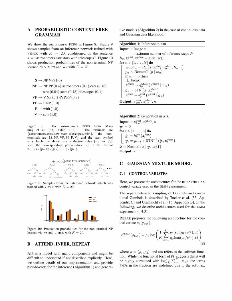
We show the astronomers PCFG in Figure 8. Figure 9shows samples from an inference network trained withVIMCO with K = 20, conditioned on the sentencex = “astronomers saw stars with telescopes”. Figure 10shows production probabilities of the non-terminal NPlearned by VIMCO and WS with K = 20.

S→ NP VP (1.0)

NP→ NP PP (0.4)|astronomers (0.1)|ears (0.18)|saw (0.04)|stars (0.18)|telescopes (0.1)

VP→ V NP (0.7)|VP PP (0.3)

PP→ P NP (1.0)

P→ with (1.0)

V→ saw (1.0).

Figure 8: The astronomers PCFG from Man-ning et al. [35, Table 11.2]. The terminals are{astronomers, ears, saw, stars, telescopes,with}, the non-terminals are {S,NP,VP, PP, P,V} and the start symbolis S. Each row above lists production rules {ni → ζj}with the corresponding probabilities pij in the formatni → ζ1 (pi1)|ζ2 (pi2)| · · · |ζJ (piJ).

S

NP

stars

VP

V

saw

NP

stars

S

NP

stars

VP

V

saw

NP

astronomers

S

NP

ears

VP

V

saw

NP

stars

S

NP

stars

VP

V

saw

NP

saw

S

NP

ears

VP

V

saw

NP

ears

0:029 0:021 0:016 0:015 0:015

qVIMCO(parse treejsentence)

Figure 9: Samples from the inference network which wastrained with VIMCO with K = 20.

NP PP astronomers ears saw stars telescopes0.0

0.5

P(N

P)

TrueWSVIMCO

Figure 10: Production probabilities for the non-terminal NPlearned via WS and VIMCO with K = 20.

B ATTEND, INFER, REPEAT

AIR is a model with many components and might bedifficult to understand if not described explicitly. Here,we outline details of our implementation and providepseudo-code for the inference (Algorithm 1) and genera-

tive models (Algorithm 2) in the case of continuous dataand Gaussian data likelihood.

Algorithm 1: Inference in AIR

Input : Image x,maximum number of inference steps N

h0, zwhat0 , zwhere

0 = initialize()for n ∈ [1, . . . , N ] do

wn,hn = Rφ(x, zwhat

n−1, zwheren−1 ,hn−1

)pn ∼ Bernoulli(p | wn)if pn = 0 then

breakzwheren ∼ qwhere

φ

(zwhere | wn

)gn = STN

(x, zwhere

n

)zwhatn ∼ qwhat

φ

(zwhat | gn

)Output: zwhat

1:n , zwhere1:n , n

Algorithm 2: Generation in AIR

Input : zwhat1:n , zwhere

1:n , ny0 = 0for t ∈ [1, . . . , n] do

gt = hdecθ

(zwhatt

)yt = yt−1 + STN−1

(gt, z

wheret

)x ∼ Normal

(x | yn, σ2

xI)

Output: x

C GAUSSIAN MIXTURE MODEL

C.1 CONTROL VARIATES

Here, we present the architectures for the REBAR/RELAXcontrol variate used in the GMM experiment.

The reparameterized sampling of Gumbels and condi-tional Gumbels is described by Tucker et al. [53, Ap-pendix C] and Grathwohl et al. [16, Appendix B]. In thefollowing, we describe architectures used for the GMMexperiment (§ 4.3).

REBAR proposes the following architecture for the con-trol variate cρ(g1:K):

cREBARρ (g1:K) = ρ1 log

(1

K

K∑k=1

pθ(sm(gk/eρ2), x)

qφ(sm(gk/eρ2)|x)

),

(8)

where ρ = (ρ1, ρ2), and sm refers to the softmax func-tion. While the functional form of (8) suggests that it willbe highly correlated with log( 1

K

∑Kk=1 wk), the terms

PMFs in the fraction are undefined due to the softmax.

A straightforward fix is to evaluate “a soft PMF” instead:

pθ(sm(gk/eρ2), x)

= pθ(sm(gk/eρ2))p(x|sm(gk/e

ρ2))

= Categorical(sm(gk/eρ2)|sm(θ))·

Normal(x|µsm(gk/eρ2 ), σ2sm(gk/eρ2 )

)

≈ sm(gk/eρ2)ᵀsm(θ)·

Normal(x|µᵀsm(gk/eρ2), (σ2)ᵀsm(gk/e

ρ2)),

qφ(sm(gk/eρ2)|x)

= Categorical(sm(gk/eρ2)|sm(ηφ(x)))

≈ sm(gk/eρ2)ᵀsm(ηφ(x)).

Optimization of the log-temperature ρ2 is highly sensi-tive as low values can make the training unstable.

RELAX proposes using an arbitrary neural network forcρ(g1:K). Due to the symmetry in the arguments, wepick the following for the GMM experiment:

cRELAXρ (g1:K) =

1

K

K∑k=1

MLPρ([x, gk]), (9)

where the architecture of the MLP is (1 + C)-16-16-1(with the tanh nonlinearity between layers) and ρ are theweights are its weights. This architecture is—unlike theone in (8)—well-defined for all inputs. A drawback ofusing such control variate is that it can start out not beingvery correlated with log( 1

K

∑Kk=1 wk).

RELAX also proposes using a summation of the free-form control variate like the one in (9) and a more corre-lated control variate in (8).

We have tried all architectures and found that (9) leads tothe most stable and best training.

Using REBAR/RELAX for more complicated models ispossible, however designing an architecture that is highlycorrelated with the high-variance term and stable to trainstill remains a challenge.

C.2 ADDITIONAL RESULTS

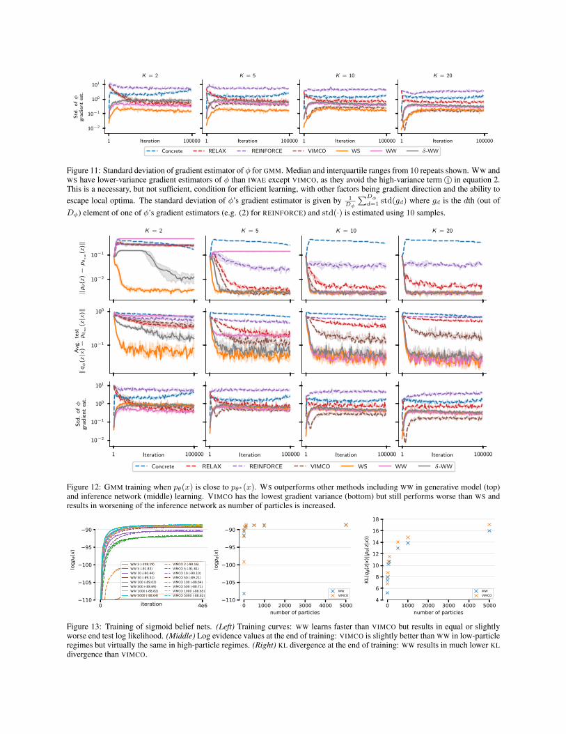
Here, we include additional GMM experiments: one forstudying φ’s gradient variance (Figure 11), the other forcomparing performances of the generative model and in-ference networks when θ is initialized closer to θ∗ thanin the main paper (Figure 12).

WW and WS have lower variance gradient estimatorsthan IWAE, except VIMCO. This is because φ’s gradi-ent estimators for WW and WS do not include the high-variance term 1 in (2). This is a necessary but not suffi-cient condition for efficient learning with other importantfactors being gradient direction and the ability to escapelocal optima. Employing the Concrete distribution gives

low-variance gradients for φ to begin with, but the modellearns poorly due to the high gradients bias (due to hightemperature hyperparameter).

In Figure 12, we initialize θ so that the mixture probabil-ities are constant. This means that the data bias is smallerthan in the main paper’s setting. With smaller data bias,we expect WS to perform better. This is empirically veri-fied since WS outperforms other methods, including WW.

D SIGMOID BELIEF NETWORKS

In Figure 13, we show training of sigmoid belief net-works with three stochastic layers with the same archi-tecture as in Mnih and Rezende [38]. We additionallydrive number of particles up to K = 5000 and includeKL plots. We find that in high particle regimes, modellearning is virtually the same for WW and VIMCO. How-ever, WW outperforms VIMCO in terms of inference net-work learning.

E DISCRETE VAES

Rolfe 2016 [48] introduces discrete VAE (DVAE). Itcombines a prior over binary latent variables with anelement-wise spike-and-X smoothing transformation, al-lowing approximate marginalization of the discrete vari-ables. This results in a continuous relaxation of discretevariables and a low-variance gradient estimator. Vah-dat et al. [56] replaced the original transformation withan overlapping exponential transformation, leading to ayet lower-variance gradient estimator. While both ap-proaches produce relaxed binary variables, the relaxationis significantly less tight ([56], Appendix C, Figure 5.)then the CONCRETE of [23, 34] Both approaches re-quire analytical inverse CDFs of the smoothing transfor-mations, a shortcoming addressed by Vahdat et al. [55]— it also leads to a tighter relaxation than its predeces-sors, however no comparison to CONCRETE is available.

DVAE was designed for undirected binary priors, e.g. re-stricted Boltzmann machines (RBM), and it does not ac-count for the case of categorical latent variables. It ispossible to construct a d-dimensional categorical vari-able from d− 1 binary variables via stick-breaking con-struction. This process is slow, however, as it requiresO(d) sequential operations and cannot be parallelized.Moreover, in the case of relaxed variables, the tightnessof the derived relaxed categorical variable decreases ex-ponentially with the number of dimensions. This is a ma-jor issue in control flows: not only we have to evaluate allbranches of the control flow, but the indicator variablesthat we multiply with outcomes of different branches be-come exponentially loose with the depth of the flow.

1 100000Iteration

10−2

10−1

100

101

Std

.o

fφ

gra

die

nt

est.

K = 2

1 100000Iteration

K = 5

Concrete RELAX REINFORCE VIMCO WS WW δ-WW

1 100000Iteration

K = 10

1 100000Iteration

K = 20

Figure 11: Standard deviation of gradient estimator of φ for GMM. Median and interquartile ranges from 10 repeats shown. WW andWS have lower-variance gradient estimators of φ than IWAE except VIMCO, as they avoid the high-variance term 1 in equation 2.This is a necessary, but not sufficient, condition for efficient learning, with other factors being gradient direction and the ability toescape local optima. The standard deviation of φ’s gradient estimator is given by 1

Dφ

∑Dφd=1 std(gd) where gd is the dth (out of

Dφ) element of one of φ’s gradient estimators (e.g. (2) for REINFORCE) and std(·) is estimated using 10 samples.

10−2

10−1

‖pθ

(z)−

pθ

tru

e(z

)‖

K = 2 K = 5 K = 10 K = 20

10−1

100

Avg

.te

st‖qφ

(z|x

)−

pθ

tru

e(z|x

)‖

1 100000Iteration

10−2

10−1

100

101

Std

.o

fφ

gra

die

nt

est.

1 100000Iteration

Concrete RELAX REINFORCE VIMCO WS WW δ-WW

1 100000Iteration 1 100000Iteration

Figure 12: GMM training when pθ(x) is close to pθ∗(x). WS outperforms other methods including WW in generative model (top)and inference network (middle) learning. VIMCO has the lowest gradient variance (bottom) but still performs worse than WS andresults in worsening of the inference network as number of particles is increased.

0 4e6iteration110

105

100

95

90

logp

(x)

WW 2 (-108.19)WW 5 (-91.83)WW 10 (-90.44)WW 50 (-89.31)WW 100 (-89.03)WW 500 (-88.69)WW 1000 (-88.82)WW 5000 (-88.64)

VIMCO 2 (-99.16)VIMCO 5 (-91.61)VIMCO 10 (-90.10)VIMCO 50 (-89.21)VIMCO 100 (-88.64)VIMCO 500 (-88.71)VIMCO 1000 (-88.65)VIMCO 5000 (-88.62)

0 1000 2000 3000 4000 5000number of particles

110

105

100

95

90

logp

(x)

WWVIMCO

0 1000 2000 3000 4000 5000number of particles

4

6

8

10

12

14

16

18

KL(q

(z|x

)||p

(z|x

))

WWVIMCO

Figure 13: Training of sigmoid belief nets. (Left) Training curves: WW learns faster than VIMCO but results in equal or slightlyworse end test log likelihood. (Middle) Log evidence values at the end of training: VIMCO is slightly better than WW in low-particleregimes but virtually the same in high-particle regimes. (Right) KL divergence at the end of training: WW results in much lower KLdivergence than VIMCO.