REVISITING OPTIMAL DELAUNAY TRIANGULATION FOR 3D … · Delaunay consistence. Due to its shape...

SIAM J. SCI. COMPUT. c© 2014 Society for Industrial and Applied MathematicsVol. 36, No. 3, pp. A930–A954

REVISITING OPTIMAL DELAUNAY TRIANGULATION FOR 3DGRADED MESH GENERATION∗

ZHONGGUI CHEN† , WENPING WANG‡ , BRUNO LEVY§ , LIGANG LIU¶, AND

FENG SUN‡

Abstract. This paper proposes a new algorithm to generate a graded three-dimensional tetrahe-dral mesh. It revisits the class of methods based on optimal Delaunay triangulation (ODT) and pro-poses a proper way of injecting a background density function into the objective function minimizedby ODT. This continuous/analytic point of view leads to an objective function that is continuous andDelaunay consistent, in contrast with the discrete/geometrical point of view developed in previouswork. To optimize the objective function, this paper proposes a hybrid algorithm that combines alocal search (quasi-Newton) with a global optimization (simulated annealing). The benefits of themethod are both improved performances and an improved quality of the result in terms of dihedralangles. This results from the combination of two effects. First, the local search has a faster speedof convergence than previous work due to the better behavior of the objective function, and second,the algorithm avoids getting stuck in a poor local minimum. Experimental results are evaluated andcompared using standard metrics.

Key words. mesh generation, optimal Delaunay triangulation, centroidal Voronoi tessellation,slivers, mesh optimization

AMS subject classifications. 42A10, 41A25, 41A50, 65N50

DOI. 10.1137/120875132

1. Introduction. The quality of a tetrahedral mesh can tremendously affect theaccuracy and efficiency of a finite element simulation [27]. A large body of work existsfor generating tetrahedral meshes. Among these, the optimization-based methods—also called variational by some authors—have attracted much attention as they arecapable of handling domains of complex shapes and topology in a consistent man-ner based on energy minimization. In this paper, we study the optimal Delaunaytriangulation (ODT) for three-dimensional (3D) graded mesh generation.

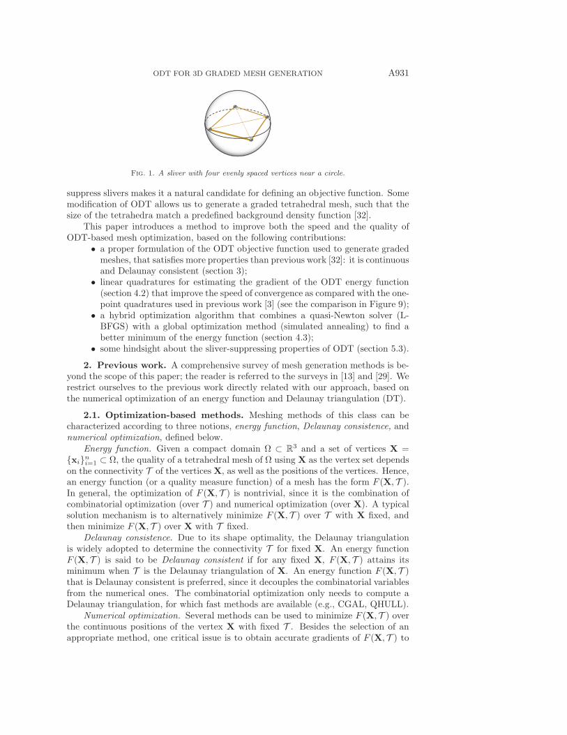
ODT is defined as the minimizer of an objective function [2]. It has been shown [1]to be very effective in suppressing slivers, which are tetrahedra with near-zero volumebut quite proper faces; for example, four evenly spaced vertices near a great circleof a sphere give rise to a sliver, as shown in Figure 1. Slivers have very small (nearzero) and very large (near π) dihedral angles, which cause poor numerical conditionsin simulation and are notoriously hard to remove. Hence, the ability of ODT to

∗Submitted to the journal’s Methods and Algorithms for Scientific Computing section April 27,2012; accepted for publication (in revised form) February 21, 2014; published electronically May 13,2014.

http://www.siam.org/journals/sisc/36-3/87513.html†Department of Computer Science, Xiamen University, Xiamen, 361005 China, and University of

Hong Kong, Hong Kong, China ([email protected]). Part of this work was done while theauthor was visiting the University of Hong Kong. This author was supported by NSFC 61100107,NSFC 61100105, and the Natural Science Foundation of Fujian Province of China (2012J01291,2011J05007).

‡Department of Computer Science, University of Hong Kong, Hong Kong, China ([email protected], [email protected]). The second author was supported by the National Basic ResearchProgram of China (2011CB302400), NSFC 61272019, NSFC 61332015, and the Research GrantCouncil of Hong Kong (718209, 718010, 718311, 717012).

§Project ALICE, INRIA, Villers les Nancy, 54600 France ([email protected]).¶School of Mathematical Sciences, University of Science and Technology of China, Hefei, 230026

China ([email protected]). This author was supported by NSF 61222206 and One Hundred TalentProject of the Chinese Academy of Sciences.

A930

http://www.siam.org/journals/sisc/36-3/87513.html

mailto:[email protected]






ODT FOR 3D GRADED MESH GENERATION A931

Fig. 1. A sliver with four evenly spaced vertices near a circle.

suppress slivers makes it a natural candidate for defining an objective function. Somemodification of ODT allows us to generate a graded tetrahedral mesh, such that thesize of the tetrahedra match a predefined background density function [32].

This paper introduces a method to improve both the speed and the quality ofODT-based mesh optimization, based on the following contributions:

• a proper formulation of the ODT objective function used to generate gradedmeshes, that satisfies more properties than previous work [32]: it is continuousand Delaunay consistent (section 3);• linear quadratures for estimating the gradient of the ODT energy function(section 4.2) that improve the speed of convergence as compared with the one-point quadratures used in previous work [3] (see the comparison in Figure 9);• a hybrid optimization algorithm that combines a quasi-Newton solver (L-BFGS) with a global optimization method (simulated annealing) to find abetter minimum of the energy function (section 4.3);• some hindsight about the sliver-suppressing properties of ODT (section 5.3).

2. Previous work. A comprehensive survey of mesh generation methods is be-yond the scope of this paper; the reader is referred to the surveys in [13] and [29]. Werestrict ourselves to the previous work directly related with our approach, based onthe numerical optimization of an energy function and Delaunay triangulation (DT).

2.1. Optimization-based methods. Meshing methods of this class can becharacterized according to three notions, energy function, Delaunay consistence, andnumerical optimization, defined below.

Energy function. Given a compact domain Ω ⊂ R3 and a set of vertices X =

{xi}ni=1 ⊂ Ω, the quality of a tetrahedral mesh of Ω using X as the vertex set dependson the connectivity T of the vertices X, as well as the positions of the vertices. Hence,an energy function (or a quality measure function) of a mesh has the form F (X, T ).In general, the optimization of F (X, T ) is nontrivial, since it is the combination ofcombinatorial optimization (over T ) and numerical optimization (over X). A typicalsolution mechanism is to alternatively minimize F (X, T ) over T with X fixed, andthen minimize F (X, T ) over X with T fixed.

Delaunay consistence. Due to its shape optimality, the Delaunay triangulationis widely adopted to determine the connectivity T for fixed X. An energy functionF (X, T ) is said to be Delaunay consistent if for any fixed X, F (X, T ) attains itsminimum when T is the Delaunay triangulation of X. An energy function F (X, T )that is Delaunay consistent is preferred, since it decouples the combinatorial variablesfrom the numerical ones. The combinatorial optimization only needs to compute aDelaunay triangulation, for which fast methods are available (e.g., CGAL, QHULL).

Numerical optimization. Several methods can be used to minimize F (X, T ) overthe continuous positions of the vertex X with fixed T . Besides the selection of anappropriate method, one critical issue is to obtain accurate gradients of F (X, T ) to

A932 Z. CHEN, W. WANG, B. LEVY, L. LIU, AND F. SUN

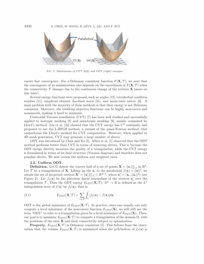
Fig. 2. Illustrations of CVT (left) and ODT (right) energies.

ensure fast convergence. For a Delaunay consistent function F (X, T ), we note thatthe convergence of its minimization also depends on the smoothness of F (X, T ) whenthe connectivity T changes due to the continuous change of the vertices X (more onthis later).

Several energy functions were proposed, such as angles [12], tetrahedral conditionnumber [11], simplicial element Jacobian norm [21], and mean-ratio metric [6]. Amain problem with the majority of these methods is that their energy is not Delaunayconsistent. Moreover, the resulting objective functions can be highly nonconvex andnonsmooth, making it hard to minimize.

Centroidal Voronoi tessellation (CVT) [7] has been well studied and successfullyapplied to isotropic meshing [8] and anisotropic meshing [9], mainly computed byLloyd’s method. Liu et al. [22] showed that the CVT energy has C2 continuity andproposed to use the L-BFGS method, a variant of the quasi-Newton method, thatoutperforms the Lloyd’s method for CVT computation. However, when applied to3D mesh generation, CVT may generate a large number of slivers.

ODT was introduced by Chen and Xu [5]. Alliez et al. [1] observed that the ODTmethod performs better than CVT in terms of removing slivers. This is because theODT energy directly measures the quality of a triangulation, while the CVT energyis formulated in terms of its dual structure (Voronoi diagram) and therefore does notpenalize slivers. We now review the uniform and weighted cases.

2.2. Uniform ODT.Definition. Let Ω denote the convex hull of a set of points X = {xi}ni=1 in R

d.Let T be a triangulation of X. Lifting up the xi to the paraboloid f(x) = ‖x‖2, weobtain the set of projected vertices X′ = {x′

i}ni=1 ⊂ Rd+1, where x′

i = (xi, ‖xi‖2) (seeFigure 2). Let fI(x) be the piecewise linear interpolant of the vertices x′

i over thetriangulation T . Then the ODT energy EODT(X, T ): Ωn → R is defined as the L1

interpolation error of f(x) by fI(x), that is,

EODT(X, T ) =∑τ∈T

∫τ

|fI(x)− f(x)|dx.(2.1)

ODT is the global minimizer of EODT(X, T ). In practice, since one usually can onlycompute a local minimizer of the nonconvex function EODT(X), we will still use theterm “ODT” to refer to a triangulation given by a local minimizer of EODT(X). Then,our goal is to minimize EODT(X, T ) to compute a triangulation of the domain Ω, withthe positions of the sites X and their connectivity subject to optimization.

Property. EODT(X, T ) is Delaunay consistent [5]. This follows from the obser-vation that the volume EODT(X, T ) is minimized when the polyhedron of fI(x) is


the lower convex hull CH(X′) of X′ = {x′i}i=1 and the fact that the Delaunay trian-

gulation of X is the projection of CH(X′) onto Rd (see Figure 2). Consequently, we

will omit the triangulation T in EODT(X, T ) and always use the DT of X by default,since we are primarily interested in the minimization of EODT(X, T ).

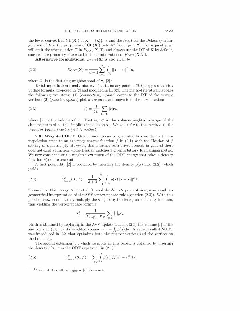
Alternative formulations. EODT(X) is also given by

EODT(X) =1

d+ 3

n∑i=1

∫Ωi

‖x− xi‖2dx,(2.2)

where Ωi is the first-ring neighborhood of xi [2].1

Existing solution mechanisms. The stationary point of (2.2) suggests a vertexupdate formula, proposed in [2] and modified in [1, 32]. The method iteratively appliesthe following two steps: (1) (connectivity update) compute the DT of the currentvertices; (2) (position update) pick a vertex xi and move it to the new location:

x∗i =

1

|Ωi|∑τ∈Ωi

|τ |ck,(2.3)

where |τ | is the volume of τ . That is, x∗i is the volume-weighted average of the

circumcenters of all the simplices incident to xi. We will refer to this method as theaveraged Voronoi vertex (AVV) method.

2.3. Weighted ODT. Graded meshes can be generated by considering the in-terpolation error to an arbitrary convex function f in (2.1) with the Hessian of fserving as a metric [4]. However, this is rather restrictive, because in general theredoes not exist a function whose Hessian matches a given arbitrary Riemannian metric.We now consider using a weighted extension of the ODT energy that takes a densityfunction ρ(x) into account.

A first possibility [2] is obtained by inserting the density ρ(x) into (2.2), whichyields

EρODT(X, T ) = 1

d+ 3

n∑i=1

∫Ωi

ρ(x)‖x− xi‖2dx.(2.4)

To minimize this energy, Alliez et al. [1] used the discrete point of view, which makes ageometrical interpretation of the AVV vertex update rule (equation (2.3)). With thispoint of view in mind, they multiply the weights by the background density function,thus yielding the vertex update formula

x∗i =

1∑τ∈Ωi

|τ |ρ∑τ∈Ωi

|τ |ρck,

which is obtained by replacing in the AVV update formula (2.3) the volume |τ | of thesimplex τ in (2.3) by its weighted volume |τ |ρ =

∫τ ρ(x)dσ. A variant called NODT

was introduced in [32] that optimizes both the interior vertices and the vertices onthe boundary.

The second extension [3], which we study in this paper, is obtained by insertingthe density ρ(x) into the ODT expression in (2.1):

EρODT(X, T ) =

∑τ∈T

∫τ

ρ(x)|fI(x) − x2|dx.(2.5)

1Note that the coefficient 1d+1

in [2] is incorrect.


Density

0.1

10.1

0 0.2 0.4 0.6 0.8 1

0.35

0.4

0.45

0.5

( )E

t

Fig. 3. Empirical comparison of the continuity of CVT (C2 but generates slivers), EρODT

(discontinuous), and energy EρODT (C0 but not C1). The Delaunay triangulation is used by default

in EρODT and Eρ

ODT.

The gradient and Hessian matrix of this energy function are difficult to compute.For this reason, Chen and Holst [3] proposed a one-point quadrature to estimate thegradient and the Hessian matrix, and they minimize the energy with Newton-typeiterations. We propose a better approximation of the gradient, leading to a moreefficient solution mechanism.

3. Revisiting weighted ODT. The two extensions EρODT (2.4) and Eρ

ODT (2.5)are identical if the density function ρ(x) is constant. For general density, there aresome important differences.

As shown in Figure 3, we conducted a simple numerical experiment with atwo-dimensional (2D) triangulation of eight vertices. One of the vertices movesalong a straight line parameterized by t, and we plot the different energies (CVT,Eρ

ODT(X, DT ), and EρODT(X, DT )) as a function of t to compare their continuity. The

EρODT in (2.4), in general, is not Delaunay consistent. Moreover, it is not continuous

when the Delaunay triangulation of the variable point set X changes its connectivity.Besides these empirical observations, we now further characterize the properties ofEρ

ODT and prove the following properties.Theorem 3.1. The ODT function Eρ

ODT in (2.5) is Delaunay consistent.Proof. Let f∗

I (x) be the piecewise linear interpolant of f(x) = x2 based on theDelaunay triangulation DT (X) of X. Let fI(x) be a piecewise linear interpolationof f(x) based on any triangulation T of DT (X). Since f∗

I (x) is given by the lowerconvex hull of the lifted points X′ on the paraboloid, for any point x in the domain,we have

fI(x)− f(x) ≥ f∗I (x) − f(x) ≥ 0.

It follows that

ρ(x)|fI(x)− f(x)| ≥ ρ(x)|f∗I (x)− f(x)|.

Hence,

DT (X) = argminT

EρODT(X, T ).

This completes the proof.In other words, for a fixed X, the optimal triangulation that minimizes the ODT

energy function among all triangulations is the Delaunay triangulation. This deter-mines the combinatorial parameters T , and we can now consider that Eρ

ODT onlydepends on X.


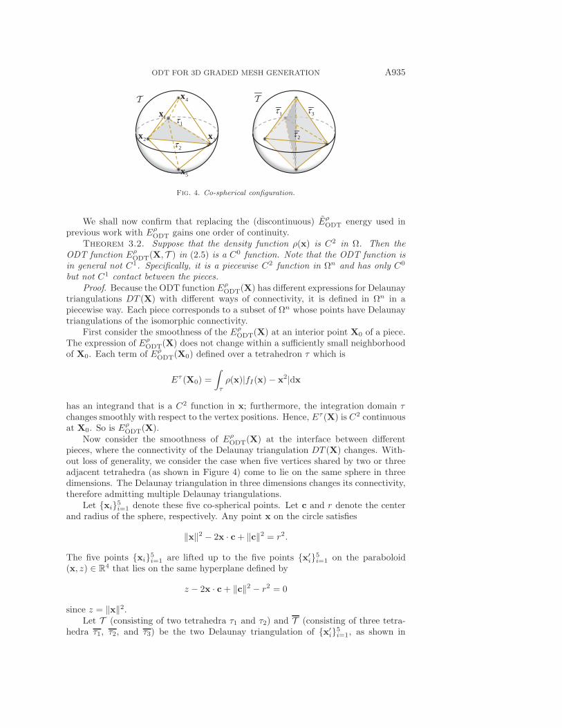
1x

2x 3x

4x

5x

1

2

1

2

3

Fig. 4. Co-spherical configuration.

We shall now confirm that replacing the (discontinuous) EρODT energy used in

previous work with EρODT gains one order of continuity.

Theorem 3.2. Suppose that the density function ρ(x) is C2 in Ω. Then theODT function Eρ

ODT(X, T ) in (2.5) is a C0 function. Note that the ODT function isin general not C1. Specifically, it is a piecewise C2 function in Ωn and has only C0

but not C1 contact between the pieces.Proof. Because the ODT function Eρ

ODT(X) has different expressions for Delaunaytriangulations DT (X) with different ways of connectivity, it is defined in Ωn in apiecewise way. Each piece corresponds to a subset of Ωn whose points have Delaunaytriangulations of the isomorphic connectivity.

First consider the smoothness of the EρODT(X) at an interior point X0 of a piece.

The expression of EρODT(X) does not change within a sufficiently small neighborhood

of X0. Each term of EρODT(X0) defined over a tetrahedron τ which is

Eτ (X0) =

∫τ

ρ(x)|fI(x) − x2|dx

has an integrand that is a C2 function in x; furthermore, the integration domain τchanges smoothly with respect to the vertex positions. Hence, Eτ (X) is C2 continuousat X0. So is Eρ

ODT(X).Now consider the smoothness of Eρ

ODT(X) at the interface between differentpieces, where the connectivity of the Delaunay triangulation DT (X) changes. With-out loss of generality, we consider the case when five vertices shared by two or threeadjacent tetrahedra (as shown in Figure 4) come to lie on the same sphere in threedimensions. The Delaunay triangulation in three dimensions changes its connectivity,therefore admitting multiple Delaunay triangulations.

Let {xi}5i=1 denote these five co-spherical points. Let c and r denote the centerand radius of the sphere, respectively. Any point x on the circle satisfies

‖x‖2 − 2x · c+ ‖c‖2 = r2.

The five points {xi}5i=1 are lifted up to the five points {x′i}5i=1 on the paraboloid

(x, z) ∈ R4 that lies on the same hyperplane defined by

z − 2x · c+ ‖c‖2 − r2 = 0

since z = ‖x‖2.Let T (consisting of two tetrahedra τ1 and τ2) and T (consisting of three tetra-

hedra τ1, τ2, and τ3) be the two Delaunay triangulation of {x′i}5i=1, as shown in


Figure 4. Clearly, the function fI(x) evaluated using these two triangulations has thesame value, because the lifted points {x′

i}5i=1 are coplanar in the space. It follows that

Eτ1(X0) + Eτ2(X0) = Eτ1(X0) + Eτ2(X0) + Eτ3(X0).

That is, the different expressions of the ODT function given by two adjacent pieceshave equal values at their interface. Hence, the ODT function is a C0 function. Thefact that it is not C1 is easily established by numerical verification using a specificexample. We will skip the details here.

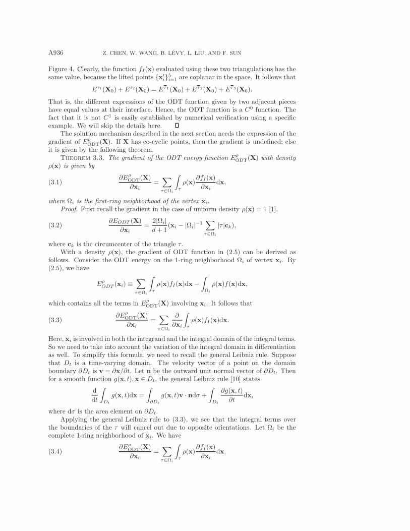
The solution mechanism described in the next section needs the expression of thegradient of Eρ

ODT(X). If X has co-cyclic points, then the gradient is undefined; elseit is given by the following theorem.

Theorem 3.3. The gradient of the ODT energy function EρODT(X) with density

ρ(x) is given by

∂EρODT(X)

∂xi=∑τ∈Ωi

∫τ

ρ(x)∂fI(x)

∂xidx,(3.1)

where Ωi is the first-ring neighborhood of the vertex xi.Proof. First recall the gradient in the case of uniform density ρ(x) = 1 [1],

∂EODT (X)

∂xi=

2|Ωi|d+ 1

(xi − |Ωi|−1∑τ∈Ωi

|τ |ck),(3.2)

where ck is the circumcenter of the triangle τ .With a density ρ(x), the gradient of ODT function in (2.5) can be derived as

follows. Consider the ODT energy on the 1-ring neighborhood Ωi of vertex xi. By(2.5), we have

EρODT (xi) ≡

∑τ∈Ωi

∫τ

ρ(x)fI(x)dx −∫Ωi

ρ(x)f(x)dx,

which contains all the terms in EρODT(X) involving xi. It follows that

∂EρODT(X)

∂xi=∑τ∈Ωi

∂

∂xi

∫τ

ρ(x)fI(x)dx.(3.3)

Here, xi is involved in both the integrand and the integral domain of the integral terms.So we need to take into account the variation of the integral domain in differentiationas well. To simplify this formula, we need to recall the general Leibniz rule. Supposethat Dt is a time-varying domain. The velocity vector of a point on the domainboundary ∂Dt is v = ∂x/∂t. Let n be the outward unit normal vector of ∂Dt. Thenfor a smooth function g(x, t),x ∈ Dt, the general Leibniz rule [10] states

d

dt

∫Dt

g(x, t)dx =

∫∂Dt

g(x, t)v · ndσ +

∫Dt

∂g(x, t)

∂tdx,

where dσ is the area element on ∂Dt.Applying the general Leibniz rule to (3.3), we see that the integral terms over

the boundaries of the τ will cancel out due to opposite orientations. Let Ωi be thecomplete 1-ring neighborhood of xi. We have

∂EρODT(X)

∂xi=∑τ∈Ωi

∫τ

ρ(x)∂fI(x)

∂xidx.(3.4)


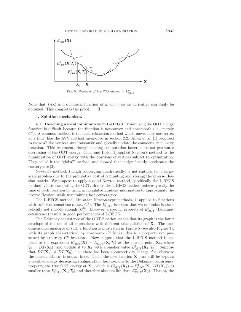
X0X 1X

( )ODTE X

1ODT 0( , )E X

1ODT2 ( , )E X

Fig. 5. Behavior of L-BFGS applied to EρODT.

Note that fI(x) is a quadratic function of xi on τ , so its derivative can easily beobtained. This completes the proof.

4. Solution mechanism.

4.1. Reaching a local minimum with L-BFGS. Minimizing the ODT energyfunction is difficult because the function is nonconvex and nonsmooth (i.e., merelyC0). A common method is the local relaxation method which moves only one vertexat a time, like the AVV method mentioned in section 2.2. Alliez et al. [1] proposedto move all the vertices simultaneously and globally update the connectivity in everyiteration. This treatment, though making computation faster, does not guaranteedecreasing of the ODT energy. Chen and Holst [3] applied Newton’s method to theminimization of ODT energy with the positions of vertices subject to optimization.They called it the “global” method, and showed that it significantly accelerates theconvergence [3].

Newton’s method, though converging quadratically, is not suitable for a large-scale problem due to the prohibitive cost of computing and storing the inverse Hes-sian matrix. We propose to apply a quasi-Newton method, specifically the L-BFGSmethod [24], to computing the ODT. Briefly, the L-BFGS method reduces greatly thetime of each iteration by using accumulated gradient information to approximate theinverse Hessian, while maintaining fast convergence.

The L-BFGS method, like other Newton-type methods, is applied to functionswith sufficient smoothness (i.e., C2). The Eρ

ODT function that we minimize is theo-retically not smooth enough (C0). However, a specific property of Eρ

ODT (Delaunayconsistence) results in good performances of L-BFGS.

The Delaunay consistence of the ODT function means that its graph is the lowerenvelope of the set of all expressions with different triangulation of X. The one-dimensional analogue of such a function is illustrated in Figure 5 (see also Figure 3),with its graph characterized by nonconvex C0 kinks; this is a property not pos-sessed by arbitrary C0 functions. Now suppose that the L-BFGS method is ap-plied to the expression Eρ

ODT(X) = E1ODT(X, T0) at the current point X0, where

T0 = DT (X0), and update it to X1 with a smaller value E1ODT(X1, T0). Suppose

that DT (X1) �= DT (X0), i.e., there has been a connectivity change, for otherwisethe nonsmoothness is not an issue. Then, the new location X1 can still be kept asa feasible, energy decreasing configuration, because, due to the Delaunay consistencyproperty, the true ODT energy at X1, which is Eρ

ODT(X1) = E2ODT(X1, DT (X1)), is

smaller than E1ODT(X1, T0) and therefore also smaller than Eρ

ODT(X0). That is, the


L-BFGS method can safely update the variable mesh vertices X across pieces of thedomain Ωn with different connectivities and still ensure an energy decrease and fastconvergence.

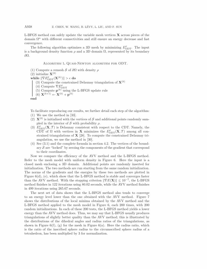
The following algorithm optimizes a 3D mesh by minimizing EρODT. The input

is a background density function ρ and a 3D domain Ω, represented by its boundary∂Ω.

Algorithm 1. Quasi-Newton algorithm for ODT.

(1) Compute a remesh S of ∂Ω with density ρ(2) initialize X(0)

while ‖∇EρODT(X

(k))‖ > ε do

(3) Compute the constrained Delaunay triangulation of X(k)

(4) Compute ∇EρODT

(5) Compute p(k) using the L-BFGS update rule(6) X(k+1) ← X(k) + p(k)

end

To facilitate reproducing our results, we further detail each step of the algorithm:

(1) We use the method in [33].(2) X(0) is initialized with the vertices of S and additional points randomly sam-

pled in the interior of S with probability ρ.(3) Eρ

ODT(X, T ) is Delaunay consistent with respect to the CDT. Namely, theCDT of Ω with vertices in X minimizes the Eρ

ODT(X, T ) among all con-strained triangulations of X [28]. To compute the constrained Delaunay tri-angulation, we use the method in [30].

(4) See (3.1) and the complete formula in section 4.2. The vertices of the bound-ary S are “locked” by zeroing the components of the gradient that correspondto their coordinates.

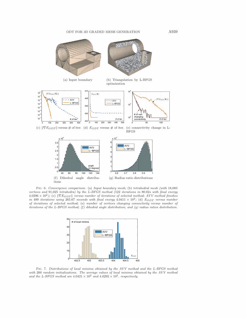
Now we compare the efficiency of the AVV method and the L-BFGS method.Refer to the mesh model with uniform density in Figure 6. Here the input is aclosed mesh enclosing a 3D domain. Additional points are randomly inserted forinitialization. The two methods are run starting from the same random initialization.The norms of the gradients and the energies by these two methods are plotted inFigure 6(d), (e), which show that the L-BFGS method is stable and converges fasterthan the AVV method. With the stopping criterion ‖∇E(X)‖ ≤ 10−7, the L-BFGSmethod finishes in 122 iterations using 80.02 seconds, while the AVV method finishesin 499 iterations using 265.67 seconds.

The next set of data shows that the L-BFGS method also tends to convergeto an energy level lower than the one obtained with the AVV method. Figure 7shows the distributions of the local minima obtained by the AVV method and theL-BFGS method applied to the mesh model in Figure 6, each 200 times, with 200random initializations. In each of these 200 tests, the L-BFGS method yields a lowerenergy than the AVV method does. Thus, we may say that L-BFGS usually producestriangulations of slightly better quality than the AVV method; this is illustrated bythe distributions of the dihedral angles and radius ratios of the triangulations, asshown in Figure 6(f), (g) for the mesh in Figure 6(a). Here the radius ratio, whichis the ratio of the inscribed sphere radius to the circumscribed sphere radius of atetrahedron, has been multiplied by 3 for normalization.


(a) Input boundary (b) Triangulation by L-BFGSoptimization

0 100 200 300 400 500

10−7

10−6

10−5

10−4

10−3

10−2

10−1

100

AVVL−BFGS

‖∇EODT(X)‖

# of iter.

(c) ‖∇EODT ‖ versus # of iter.

0 100 200 300 400 500402

404

406

408

410

AVVL−BFGS

EODT(X)

# of iter.

(d) EODT versus # of iter.

0 50 100

100

102

104

# of vert.changingconnectivity # of iter.

‖∇EODT(X)‖

(e) connectivity change in L-BFGS

40 60 80 100 120 1400

0.5

1

1.5

2

2.5

3

3.5

x 104

AVVL−BFGS

angle(in degree)

(f) Dihedral angle distribu-tions

0.6 0.7 0.8 0.9 10

1

2

3

4

5

6AVVL−BFGS

x 103

(g) Radius ratio distributions

Fig. 6. Convergence comparison. (a) Input boundary mesh; (b) tetrahedral mesh (with 18,083vertices and 91,025 tetrahedra) by the L-BFGS method (122 iterations in 80.02s with final energy4.0296 × 102); (c) ‖∇EODT ‖ versus number of iterations of selected method; AVV method finishesin 499 iterations using 265.67 seconds with final energy 4.0411 × 102; (d) EODT versus numberof iterations of selected method; (e) number of vertices changing connectivity versus number ofiterations of the L-BFGS method; (f) dihedral angle distribution; and (g) radius ratios distribution.

402.5 403 403.5 404 404.5 4050

10

20

30

40

50

AVVL−BFGS

# of local minima

EODT

Fig. 7. Distributions of local minima obtained by the AVV method and the L-BFGS methodwith 200 random initializations. The average values of local minima obtained by the AVV methodand the L-BFGS method are 4.0421× 102 and 4.0292 × 102, respectively.


(a) Non-uniform triangulation

0 100 200 300 400 500 600

10

10

10

10

10

AVV

# of iter.

|| EODT(X)||

(b) Gradient graphs

0 200 400 600

0.018

0.0181

0.0182

0.0183 AVVEODT(X)

# of iter.

(c) Energy graphs

400 450 500 550 6001.8133

1.8134

1.8135

1.8136

1.8137

1.8138

1.8139

# of iter.

EODT(X)

x 10-2

(d) Zoom-in view

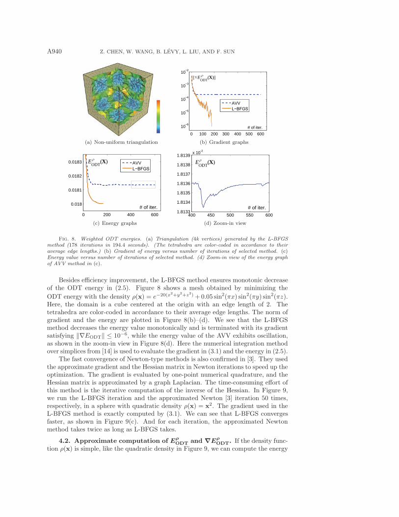
Fig. 8. Weighted ODT energies. (a) Triangulation (4k vertices) generated by the L-BFGSmethod (178 iterations in 194.4 seconds). (The tetrahedra are color-coded in accordance to theiraverage edge lengths.) (b) Gradient of energy versus number of iterations of selected method. (c)Energy value versus number of iterations of selected method. (d) Zoom-in view of the energy graphof AVV method in (c).

Besides efficiency improvement, the L-BFGS method ensures monotonic decreaseof the ODT energy in (2.5). Figure 8 shows a mesh obtained by minimizing the

ODT energy with the density ρ(x) = e−20(x2+y2+z2) +0.05 sin2(πx) sin2(πy) sin2(πz).Here, the domain is a cube centered at the origin with an edge length of 2. Thetetrahedra are color-coded in accordance to their average edge lengths. The norm ofgradient and the energy are plotted in Figure 8(b)–(d). We see that the L-BFGSmethod decreases the energy value monotonically and is terminated with its gradientsatisfying ‖∇EODT‖ ≤ 10−6, while the energy value of the AVV exhibits oscillation,as shown in the zoom-in view in Figure 8(d). Here the numerical integration methodover simplices from [14] is used to evaluate the gradient in (3.1) and the energy in (2.5).

The fast convergence of Newton-type methods is also confirmed in [3]. They usedthe approximate gradient and the Hessian matrix in Newton iterations to speed up theoptimization. The gradient is evaluated by one-point numerical quadrature, and theHessian matrix is approximated by a graph Laplacian. The time-consuming effort ofthis method is the iterative computation of the inverse of the Hessian. In Figure 9,we run the L-BFGS iteration and the approximated Newton [3] iteration 50 times,respectively, in a sphere with quadratic density ρ(x) = x2. The gradient used in theL-BFGS method is exactly computed by (3.1). We can see that L-BFGS convergesfaster, as shown in Figure 9(c). And for each iteration, the approximated Newtonmethod takes twice as long as L-BFGS takes.

4.2. Approximate computation of EρODT and ∇Eρ

ODT. If the density func-tion ρ(x) is simple, like the quadratic density in Figure 9, we can compute the energy


(a) Initial mesh (60k vert.) (b) L-BFGS

0 10 20 30 40 50

1.2

1.3

1.4

1.5

1.6

1.7

1.8

1.9L−BFGSAppro. Newton

EODT(X)

# of iter.

�

(c) Energy graphs

Method EρODT ‖∇Eρ

ODT‖ avg. radius ratio time (sec.) per iter.L-BFGS 1.21037 1.369e-5 0.8910 3.04

Appro. Newton 1.23069 7.294e-4 0.8685 6.13

(d) Statistics of comparison

Fig. 9. Comparing L-BFGS and the approximated Newton method in [3]. The initial pointsare randomly distributed in the sphere according to the density function ρ(x) = x2.

EρODT and its gradient ∇Eρ

ODT precisely. For general density, the numerical integra-tion method in [14] can be used to approximate the integral with sufficient precision.(See the example in Figure 8.) If the density varies smoothly in a tetrahedron, wecan approximate it by linear interpolation, thus achieving fast computation.

Noting that fI(x) ≥ x2, the ODT energy in (2.5) can be written as

EρODT(X) =

∑τ∈DT (X)

∫τ

ρ(x)fI(x)dx −∫Ω

ρ(x)x2dσ.

We omit the computation of the second term in the above formula which is a constantfor a fixed domain Ω.

Theorem 4.1. Suppose a tetrahedron τ is specified by its four vertices as xi,where i = 0, . . . , 3. Approximating ρ(x) by linear interpolation in each tetrahedron,one has

(4.1)∑

τ∈DT (X)

∫τ

ρ(x)fI(x)dx ≈1

20

∑τ∈DT (X)

|τ |

⎛⎝ 3∑

i,j=0

ρiwj +

3∑i=0

ρiwi

⎞⎠,

where wi = ‖xi‖2, ρi = ρ(xi).Proof. Let λ = (λ0, λ1, λ2, λ3)

T denote the barycentric coordinate of a point x inτ ; then we have

(4.2) x =

3∑i=0

λixi, fI(x) =

3∑i=0

λiwi, ρ(x) ≈3∑

i=0

λiρi.

Plugging the above formula into the integral in (4.1), we have

∫τ

ρ(x)fI(x)dx ≈ 6|τ |3∑

i,j=0

ρiwj

∫τ

λiλjdλ(4.3)

=|τ |20

⎛⎝ 3∑

i,j=0

ρiwj +3∑

i=0

ρiwi

⎞⎠ .


The last equation is obtained by using the formula for integrating a polynomial onthe canonical tetrahedron [18],∫

τ

λα11 λα2

2 λα33 dλ =

α1!α2!α3!

(3 +∑3

i=1 αi)!,

where τ = {(λ1, λ2, λ3) ∈ R3|∑3

i=1 λi � 1;λi � 0, i = 1, 2, 3}. Summing (4.3) fromall tetrahedra gives the result.

Let (xi, yi, zi), i = 0, . . . 3, denote the coordinates of vertices xi’s of a tetrahedronτ . For any point x = (x, y, z) in tetrahedron τ , fI(x) satisfies the following equation:

(4.4) det(M) = 0, where M =

⎛⎜⎜⎜⎜⎝

x x0 x1 x2 x3

y y0 y1 y2 y3z z0 z1 z2 z3

fI(x) w0 w1 w2 w3

1 1 1 1 1

⎞⎟⎟⎟⎟⎠ .

Thus we get

fI(x) =

(M1

M4,−M2

M4,M3

M4

)· x+

M5

M4,(4.5)

where Mi is the (i, 1) minor of matrix M. We then compute ∇EρODT by the following

formula.Theorem 4.2. Approximating ρ(x) by linear interpolation in τ , one has

∂EρODT(X)

∂x0≈ 1

120

∑τ∈Ω0

(12x0|τ | −M1)

(3∑

i=0

ρi + ρ0

),(4.6)

where Ω0 is the 1-ring neighborhood of vertex x0.Proof. We first compute the derivative of fI with respect to the first coordinate

x0 of the vertex x0. From (4.5), we have

∂fI∂x0

= (m1,−m2,m3) · x+m5,(4.7)

where mi =M ′

iM4−MiM′4

M24

and M ′i = ∂Mi

∂x0. On the other hand, according to (4.5), it

obviously holds that

‖xi‖2 =

(M1

M4,−M2

M4,M3

M4

)· xi +

M5

M4, i = 0, . . . 3.

Differentiating both sides of the above equations by x0, we get{2x0 = (m1,−m2,m3) · xi +

M1

M4+m5, i = 0,

0 = (m1,−m2,m3) · xi +m5, i = 1, 2, 3.

Substituting x =∑3

i=0 xiλi into (4.7), we get

∂fI∂x0

=

(2x0 −

M1

M4

)λ0.


Recalling that ρ(x) ≈∑3

i=0 λiρi, we obtain∫τ

ρ(x)∂fI(x)

∂x0dx ≈ 6|τ |

(2x0 −

M1

M4

)∫τ

3∑i=0

ρiλiλ0dλ

=1

120(12x0|τ | −M1)

(3∑

i=0

ρi + ρ0

).

Equation (4.6) is then obtained by using formula (3.1).For the ODT function with constant density, say, ρ(x) ≡ 1, the formula (4.6)

provides another efficient way to compute the exact derivative of the ODT function,

∂EODT(X)

∂x0=

1

24

∑τ∈Ω0

(12x0|τ | −M1).

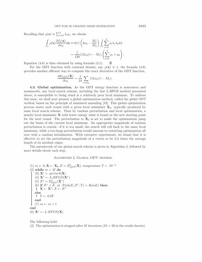
4.3. Global optimization. As the ODT energy function is nonconvex andnonsmooth, any local search scheme, including the fast L-BFGS method presentedabove, is susceptible to being stuck is a relatively poor local minimum. To addressthis issue, we shall next present a global optimization method, called the global ODTmethod, based on the principle of simulated annealing [19]. This global optimizationprocess starts each round with a given local minimizer X0, typically produced bysome local search scheme. Then by random perturbation and local optimization, anearby local minimizer X with lower energy value is found as the new starting pointfor the next round. The perturbation to X0 is set to make the optimization jumpout the basin of the current local minimum. An appropriate magnitude of randomperturbation is crucial—if it is too small, the search will roll back to the same localminimum, while a too-large perturbation would amount to restarting optimization allover with a random initialization. With extensive experiments, we found that it iseffective to set the perturbation magnitude of a vertex to be 0.2 times the averagelength of its incident edges.

The pseudocode of our global search scheme is given in Algorithm 2, followed bymore details about each step.

Algorithm 2. Global ODT method.

(1) m← 0,X← X0, E = EρODT(X), temperature T ← 10−4

(2) while m < M do(3) X∗ ← perturb(X)(4) X∗ ← L-BFGS(X∗)(5) E∗ = Eρ

ODT(X∗)

(6) if E∗ < E or Prob(E,E∗, T ) > Rand() thenX← X∗; E ← E∗

elseT ← 0.9T

end(7) m← m+ 1

end(8) X∗ ← L-BFGS(X)

The following hold:(2) The optimization is stopped afterM iterations (M = 20 in the results herein).


(3) Each vertex is perturbed along a random direction with a maximum magni-tude of 0.2 times the average length of its incident edges.

(4) We run only 20 iterations of L-BFGS (Algorithm 1, steps (3) to (6), since ahighly accurate minimizer is not necessary at this stage.

(6) X∗ is accepted as the new starting point of the next round if its ODTenergy E∗ is lower than E; otherwise X∗ is accepted with the probabilityProb(E,E∗, T ) = exp((E − E∗)/T ).

(8) Finally, 30 iterations of L-BFGS are applied again to further minimize X.

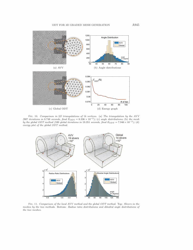
We first use a 2D mesh example to allow visual appreciation of the improvementbrought about by the global ODT method. As shown in Figure 10, starting from thesame random initialization, the 2D mesh obtained by the global ODT method (Fig-ure 10(c)) is much better than the one obtained by the AVV method (Figure 10(a)),in terms of angle distributions (Figure 10(b)). The ODT energies of the sequence oflocal minima obtained in consecutive rounds are shown in Figure 10(d).

Next we consider the 3D meshing example shown in Figure 11. Here 20 roundsof the global ODT method are applied to the mesh model in Figure 6, finishing in246.21 seconds with energy value 3.9799 × 102, which is much lower than the range[4.0341×102, 4.0432×102] of the local minima produced by 200 repeated applicationsof the AVV method, as shown in Figure 7. In comparison, the AVV result (the sameas in Figure 6) takes 499 iterations using 265.67 seconds with final energy 4.0411×102.Accordingly, the mesh quality has improved remarkably in terms of both the radiusratio and dihedral angle distributions. Furthermore, the number of slivers is furtherreduced by global optimization, even though it is already quite small by the AVVmethod.

5. Implementation and evaluation. Our algorithm is implemented in C++.We use the TetGen library [30] for generating 3D Delaunay triangulation. All theexperiments are conducted on a laptop computer with a 2.66 GHz Intel processor and4 GB memory.

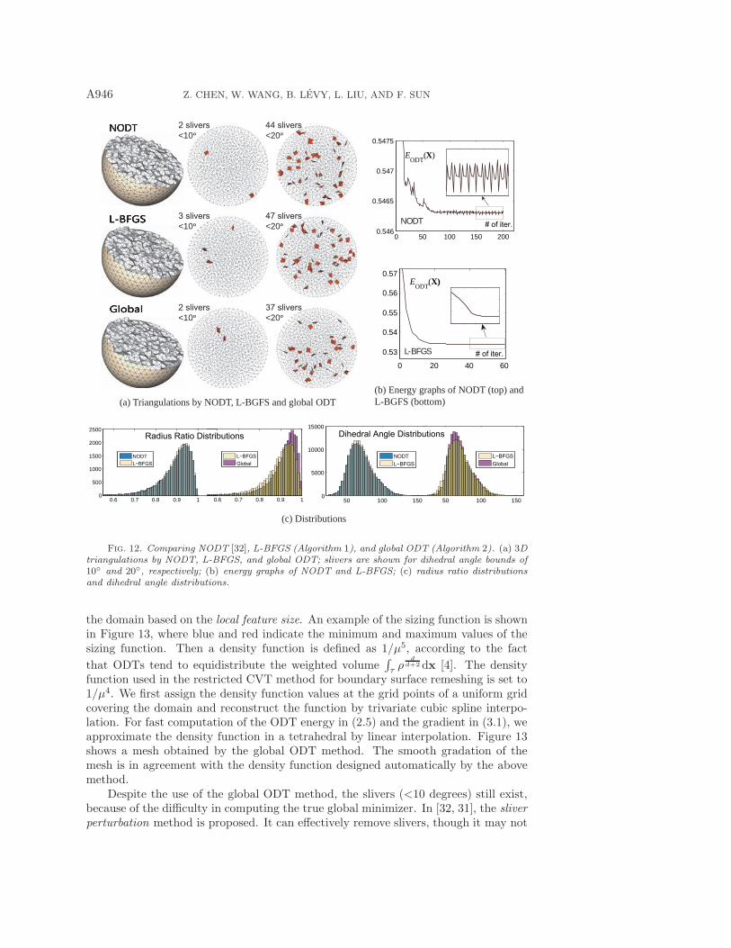
5.1. Boundary handling. A tetrahedral mesh needs to conform with the do-main boundary, which is a triangle mesh surface. Boundary handling refers to theway that those mesh vertices on the domain boundary are determined. In the NODTmethod by Tournois et al. [32], the positions of the boundary vertices are computedby maintaining the ODT circumsphere property and then projected onto the domainboundary. The biggest problem with this treatment is that the ODT energy, in gen-eral, is not decreased by an NODT iteration. To resolve this issue, we propose to firstcompute a good initial meshing of the domain boundary before minimizing the ODTenergy. We use the restricted CVT method [33] to obtain a high-quality remeshing ofthe boundary. With the boundary mesh fixed, the constrained Delaunay triangulationis used in the ODT computation.

Figure 12 shows a comparison of the NODT method, the L-BFGS method, andthe global ODT method. The global ODT method produces a triangulation of thebest quality with the smallest number of slivers. As mentioned, the NODT methoddoes not ensure the monotonic decrease of the ODT energy, as shown in Figure 12(b),and stops with the energy 0.5436, which is higher than those of the L-BFGS methodand the global ODT method, which are 0.5347 and 0.5228, respectively.

5.2. Sliver-free graded mesh. Mesh gradation is controlled by a density func-tion of the ODT energy function. We adopt the following method proposed in [1] forthe automatic design of density functions. First, a sizing function μ(x) is defined in


(a) AVV

30 40 50 60 70 80 900

200

400

600

800

1000

1200

AVVGlobal

Angle Distribution

angle(in degree)

(b) Angle distributions

(c) Global ODT

0 20 40 60 80 1000.079

0.08

0.081

0.082

0.083

0.084

# of iter.

EODT(X)

(d) Energy graph

Fig. 10. Comparison in 2D triangulations of 1k vertices. (a) The triangulation by the AVV(907 iterations in 8.748 seconds, final EODT = 8.336 × 10−2); (c) angle distributions; (b) the meshby the global ODT method (100 global iterations in 19.351 seconds, final EODT = 7.946×10−2); (d)energy plot of the global ODT method.

0.6 0.7 0.8 0.9 10

2

4

6

8

AVVGlobal

Radius Ratio Distributions

x 103

40 60 80 100 120 1400

1

2

3

4x 104

AVVGlobal

angle(in degree)

Dihedral Angle Distributions

Fig. 11. Comparison of the local AVV method and the global ODT method. Top: Slivers in themeshes by the two methods. Bottom: Radius ratio distributions and dihedral angle distributions ofthe two meshes.


0.6 0.7 0.8 0.9 10

500

1000

1500

2000

2500

NODT

0.6 0.7 0.8 0.9 1 50 100 1500

5000

10000

15000

NODT

50 100 150

0 50 100 150 2000.546

0.5465

0.547

0.5475

EODT(X)

0 20 40 60

0.53

0.54

0.55

0.56

0.57 EODT(X)

(a) Triangulations by NODT, L-BGFS and global ODT(b) Energy graphs of NODT (top) and L-BGFS (bottom)

(c) Distributions

<10 <20

<10 <20

<10 <20

NODT

L-BFGS

Fig. 12. Comparing NODT [32], L-BFGS (Algorithm 1), and global ODT (Algorithm 2). (a) 3Dtriangulations by NODT, L-BFGS, and global ODT; slivers are shown for dihedral angle bounds of10◦ and 20◦, respectively; (b) energy graphs of NODT and L-BFGS; (c) radius ratio distributionsand dihedral angle distributions.

the domain based on the local feature size. An example of the sizing function is shownin Figure 13, where blue and red indicate the minimum and maximum values of thesizing function. Then a density function is defined as 1/μ5, according to the fact

that ODTs tend to equidistribute the weighted volume∫τ ρ

dd+2dx [4]. The density

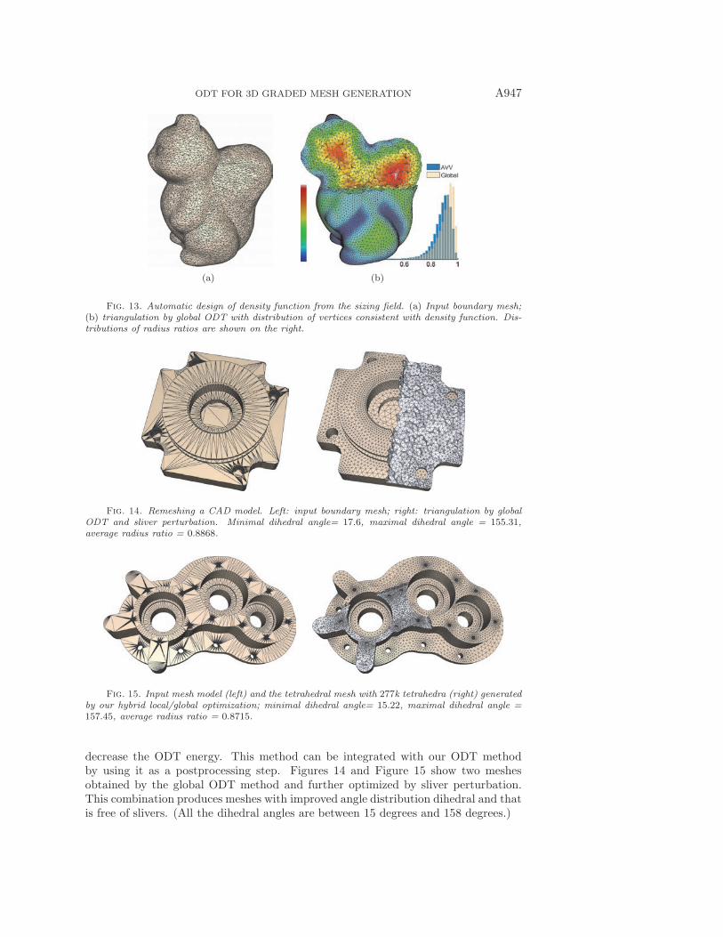
function used in the restricted CVT method for boundary surface remeshing is set to1/μ4. We first assign the density function values at the grid points of a uniform gridcovering the domain and reconstruct the function by trivariate cubic spline interpo-lation. For fast computation of the ODT energy in (2.5) and the gradient in (3.1), weapproximate the density function in a tetrahedral by linear interpolation. Figure 13shows a mesh obtained by the global ODT method. The smooth gradation of themesh is in agreement with the density function designed automatically by the abovemethod.

Despite the use of the global ODT method, the slivers (<10 degrees) still exist,because of the difficulty in computing the true global minimizer. In [32, 31], the sliverperturbation method is proposed. It can effectively remove slivers, though it may not


(a) (b)

Fig. 13. Automatic design of density function from the sizing field. (a) Input boundary mesh;(b) triangulation by global ODT with distribution of vertices consistent with density function. Dis-tributions of radius ratios are shown on the right.

Fig. 14. Remeshing a CAD model. Left: input boundary mesh; right: triangulation by globalODT and sliver perturbation. Minimal dihedral angle= 17.6, maximal dihedral angle = 155.31,average radius ratio = 0.8868.

Fig. 15. Input mesh model (left) and the tetrahedral mesh with 277k tetrahedra (right) generatedby our hybrid local/global optimization; minimal dihedral angle= 15.22, maximal dihedral angle =157.45, average radius ratio = 0.8715.

decrease the ODT energy. This method can be integrated with our ODT methodby using it as a postprocessing step. Figures 14 and Figure 15 show two meshesobtained by the global ODT method and further optimized by sliver perturbation.This combination produces meshes with improved angle distribution dihedral and thatis free of slivers. (All the dihedral angles are between 15 degrees and 158 degrees.)


(a) Interleaved (b) Global ODT (c) Stellar

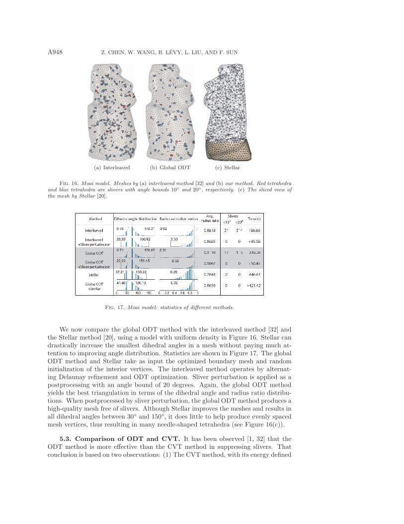
Fig. 16. Moai model. Meshes by (a) interleaved method [32] and (b) our method. Red tetrahedraand blue tetrahedra are slivers with angle bounds 10◦ and 20◦, respectively. (c) The sliced view ofthe mesh by Stellar [20].

Fig. 17. Moai model: statistics of different methods.

We now compare the global ODT method with the interleaved method [32] andthe Stellar method [20], using a model with uniform density in Figure 16. Stellar candrastically increase the smallest dihedral angles in a mesh without paying much at-tention to improving angle distribution. Statistics are shown in Figure 17. The globalODT method and Stellar take as input the optimized boundary mesh and randominitialization of the interior vertices. The interleaved method operates by alternat-ing Delaunay refinement and ODT optimization. Sliver perturbation is applied as apostprocessing with an angle bound of 20 degrees. Again, the global ODT methodyields the best triangulation in terms of the dihedral angle and radius ratio distribu-tions. When postprocessed by sliver perturbation, the global ODT method produces ahigh-quality mesh free of slivers. Although Stellar improves the meshes and results inall dihedral angles between 30◦ and 150◦, it does little to help produce evenly spacedmesh vertices, thus resulting in many needle-shaped tetrahedra (see Figure 16(c)).

5.3. Comparison of ODT and CVT. It has been observed [1, 32] that theODT method is more effective than the CVT method in suppressing slivers. Thatconclusion is based on two observations: (1) The CVT method, with its energy defined


ODT(L-BGFS)

CVT(L-BFGS)

Global ODT

20 40 60 80 1000

200

400

600

20 40 60 80 100

CVTGlobal ODT

ODTCVT

Angle Distributions

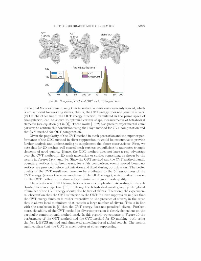
Fig. 18. Comparing CVT and ODT on 2D triangulations.

in the dual Voronoi domain, only tries to make the mesh vertices evenly spaced, whichis not sufficient for avoiding slivers; that is, the CVT energy does not penalize slivers.(2) On the other hand, the ODT energy function, formulated in the prime space oftriangulation, can be shown to optimize certain shape measurements of tetrahedralelements (see equation (7) in [1]). Those works [1, 32] also present experimental com-parisons to confirm this conclusion using the Lloyd method for CVT computation andthe AVV method for ODT computation.

Given the popularity of the CVT method in mesh generation and the superior per-formance of the ODT method in sliver suppression, it would be instructive to providefurther analysis and understanding to supplement the above observations. First, wenote that for 2D meshes, well-spaced mesh vertices are sufficient to guarantee triangleelements of good quality. Hence, the ODT method does not have a real advantageover the CVT method in 2D mesh generation or surface remeshing, as shown by theresults in Figures 18(a) and (b). Since the ODT method and the CVT method handleboundary vertices in different ways, for a fair comparison, evenly spaced boundaryvertices are provided before optimization and fixed during optimization. The betterquality of the CVT result seen here can be attributed to the C2 smoothness of theCVT energy (versus the nonsmoothness of the ODT energy), which makes it easierfor the CVT method to produce a local minimizer of good mesh quality.

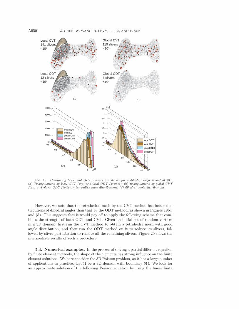
The situation with 3D triangulations is more complicated. According to the cel-ebrated Gersho conjecture [16], in theory the tetrahedral mesh given by the globalminimizer of the CVT energy should also be free of slivers. Therefore, the experimen-tal observation that the CVT is inferior to the ODT in sliver suppression implies thatthe CVT energy function is rather insensitive to the presence of slivers, in the sensethat it allows local minimizers that contain a large number of slivers. This is in linewith the conclusion in [1] that the CVT energy does not penalized slivers. Further-more, the ability of the CVT method in sliver suppression is clearly dependent on theparticular computational method used. In this regard, we compare in Figure 19 theperformance of the ODT method and the CVT method for 3D meshing, both usingthe fast L-BFGS method and simulated annealing-based global search. The resultsagain confirm that the ODT is much better at sliver suppressing.


Local CVT141 slivers<10o

Local ODT12 slivers<10o

(a)

Global CVT110 slivers<10o

Global ODT6 slivers<10o

(b)

1234

0.5

0.6

0.7

0.8

0.9

1

0

1000

2000

3000

4000

5000

local ODTlocal CVTglobal ODTglobal CVT

(c)1234

20

40

60

80

100

120

140

0

0.5

1

1.5

2

2.5

3

3.5x 10

4

local ODT

local CVT

global ODT

global CVT

(d)

Fig. 19. Comparing CVT and ODT. Slivers are shown for a dihedral angle bound of 10◦.(a) Triangulations by local CVT (top) and local ODT (bottom); (b) triangulations by global CVT(top) and global ODT (bottom); (c) radius ratio distributions; (d) dihedral angle distributions.

However, we note that the tetrahedral mesh by the CVT method has better dis-tributions of dihedral angles than that by the ODT method, as shown in Figures 19(c)and (d). This suggests that it would pay off to apply the following scheme that com-bines the strength of both ODT and CVT. Given an initial set of random verticesin a 3D domain, first run the CVT method to obtain a tetrahedra mesh with goodangle distribution, and then run the ODT method on it to reduce its slivers, fol-lowed by sliver perturbation to remove all the remaining slivers. Figure 20 shows theintermediate results of such a procedure.

5.4. Numerical examples. In the process of solving a partial different equationby finite element methods, the shape of the elements has strong influence on the finiteelement solutions. We here consider the 3D Poisson problem, as it has a large numberof applications in practice. Let Ω be a 3D domain with boundary ∂Ω. We look foran approximate solution of the following Poisson equation by using the linear finite


CVT CVT+ODT

0 0.2 0.4 0.6 0.8 10

5000

10000

15000

CVT

CVT+ODT

Radius Ratio Distributions

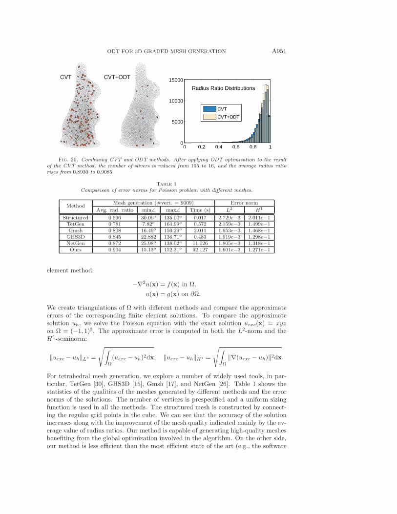
Fig. 20. Combining CVT and ODT methods. After applying ODT optimization to the resultof the CVT method, the number of slivers is reduced from 195 to 16, and the average radius ratiorises from 0.8930 to 0.9085.

Table 1

Comparison of error norms for Poisson problem with different meshes.

MethodMesh generation (#vert. = 9009) Error norm

Avg. rad. ratio min∠ max∠ Time (s) L2 H1

Structured 0.596 30.00o 135.00o 0.017 2.729e−3 2.011e−1TetGen 0.781 7.82o 164.99o 0.572 2.159e−3 1.499e−1Gmsh 0.808 16.49o 150.29o 2.011 1.953e−3 1.468e−1GHS3D 0.845 22.882 136.71o 0.483 1.919e−3 1.298e−1NetGen 0.872 25.98o 138.02o 11.026 1.805e−3 1.318e−1Ours 0.904 15.13o 152.31o 92.127 1.601e−3 1.271e−1

element method:

−∇2u(x) = f(x) in Ω,

u(x) = g(x) on ∂Ω.

We create triangulations of Ω with different methods and compare the approximateerrors of the corresponding finite element solutions. To compare the approximatesolution uh, we solve the Poisson equation with the exact solution uexc(x) = xyzon Ω = (−1, 1)3. The approximate error is computed in both the L2-norm and theH1-seminorm:

‖uexc − uh‖L2 =

√∫Ω

(uexc − uh)2dx, ‖uexc − uh‖H1 =

√∫Ω

‖∇(uexc − uh)‖2dx.

For tetrahedral mesh generation, we explore a number of widely used tools, in par-ticular, TetGen [30], GHS3D [15], Gmsh [17], and NetGen [26]. Table 1 shows thestatistics of the qualities of the meshes generated by different methods and the errornorms of the solutions. The number of vertices is prespecified and a uniform sizingfunction is used in all the methods. The structured mesh is constructed by connect-ing the regular grid points in the cube. We can see that the accuracy of the solutionincreases along with the improvement of the mesh quality indicated mainly by the av-erage value of radius ratios. Our method is capable of generating high-quality meshesbenefiting from the global optimization involved in the algorithm. On the other side,our method is less efficient than the most efficient state of the art (e.g., the software


Table 2

Running times.

Model # vert. # tet.Time (min.)

Initialization Global ODT Sliver perturbation

Figure 6 18k 91k 1.5 4.3 0.25

Figure 13 43k 206k 5.2 16.1 1.21

Figure 14 17k 82k 1.3 3.9 0.23

Figure 15 75k 404k 6.3 26.7 1.42

0 1 2 3 4 5 6 x 1050

5

10

15

20

25

30

35

DTCDT

Time (sec.)

# of vert.

Fig. 21. Comparing the time of computing CDT and DT.

GHS3D from Distene [15] or the advancing front methods in [25, 23]), due to the highcomputational complexity involved in the global optimization.

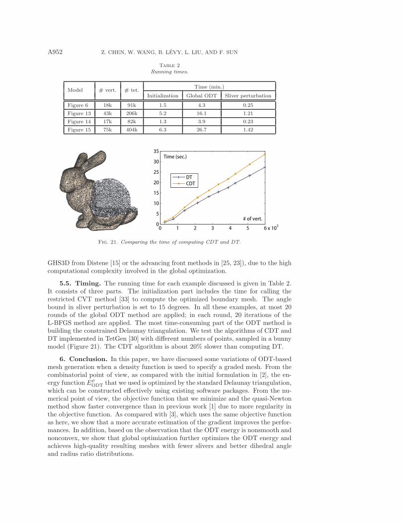
5.5. Timing. The running time for each example discussed is given in Table 2.It consists of three parts. The initialization part includes the time for calling therestricted CVT method [33] to compute the optimized boundary mesh. The anglebound in sliver perturbation is set to 15 degrees. In all these examples, at most 20rounds of the global ODT method are applied; in each round, 20 iterations of theL-BFGS method are applied. The most time-consuming part of the ODT method isbuilding the constrained Delaunay triangulation. We test the algorithms of CDT andDT implemented in TetGen [30] with different numbers of points, sampled in a bunnymodel (Figure 21). The CDT algorithm is about 20% slower than computing DT.

6. Conclusion. In this paper, we have discussed some variations of ODT-basedmesh generation when a density function is used to specify a graded mesh. From thecombinatorial point of view, as compared with the initial formulation in [2], the en-ergy function Eρ

ODT that we used is optimized by the standard Delaunay triangulation,which can be constructed effectively using existing software packages. From the nu-merical point of view, the objective function that we minimize and the quasi-Newtonmethod show faster convergence than in previous work [1] due to more regularity inthe objective function. As compared with [3], which uses the same objective functionas here, we show that a more accurate estimation of the gradient improves the perfor-mances. In addition, based on the observation that the ODT energy is nonsmooth andnonconvex, we show that global optimization further optimizes the ODT energy andachieves high-quality resulting meshes with fewer slivers and better dihedral angleand radius ratio distributions.


Considering the limitations of our method, some further research possibilities aresuggested below:

(1) The objective function EρODT introduced here together with the hybrid op-

timization algorithm improves the performance and quality of graded meshgeneration. We cannot ensure that the global minimum is obtained, but wegive experimental results that show the practical benefit of our mixed New-ton/global optimization framework. However, slivers are not totally elimi-nated, thus requiring a postprocessing with sliver perturbation [31].

(2) Our method needs to fix the vertices on the boundary. Note that a gradedmeshing of the boundary can be precomputed (e.g., using [33]). We use theconstrained Delaunay triangulation in the ODT optimization. However, theconstrained Delaunay triangulation may not exist in some extreme cases.Since the points are nearly evenly distributed in the domain during the ODToptimization, we never failed to build the constrained Delaunay triangulationsin our experiments.

(3) The objective function is C0 only, which is better than the discontinuousfunctions used in previous work but still does not fulfill the C2 theoreticalrequirement of the L-BFGS algorithm. To further improve both the speed andthe quality of the results, a unified, C2 sliver-eliminating objective functionremains to be found.

In another perspective, efficient optimization methods for anisotropic mesh gen-eration are also an important research topic.

Acknowledgment. The surface models are courtesy of Aim@Shape.

REFERENCES

[1] P. Alliez, D. Cohen-Steiner, M. Yvinec, and M. Desbrun, Variational tetrahedral meshing,ACM Trans. Graphics, 24 (2005), pp. 617–625.

[2] L. Chen, Mesh smoothing schemes based on optimal delaunay triangulations, in Proceedingsof the 13th International Meshing Roundtable, 2004, pp. 109–120.

[3] L. Chen and M. Holst, Efficient mesh optimization schemes based on optimal Delaunaytriangulations, Comput. Methods Appl. Mech. Engrg. 200 (2011), pp. 967–984.

[4] L. Chen, P. Sun, and J. Xu, Optimal anisotropic meshes for minimizing interpolation errorsin Lp norm, Math. Comp., 76 (2007), pp. 179–204.

[5] L. Chen and J. Xu, Optimal Delaunay triangulations, J. Comput. Math., 22 (2004),pp. 299–308.

[6] L. F. Diachin, P. Knupp, T. Munson, and S. Shontz, A comparison of two optimizationmethods for mesh quality improvement, Eng. Comput., 22 (2006), pp. 61–74.

[7] Q. Du, V. Faber, and M. Gunzburger, Centroidal Voronoi tessellations: Applications andalgorithms, SIAM Rev., 41 (1999), pp. 637–676.

[8] Q. Du and D. Wang, Tetrahedral mesh generation and optimization based on centroidalVoronoi tessellations, Internat. J. Numer. Methods Engrg., 56 (2003), pp. 1355–1373.

[9] Q. Du and D. Wang, Anisotropic centroidal Voronoi tessellations and their applications,SIAM J. Sci. Comput., 26 (2005), pp. 737–761.

[10] H. Flanders, Differentiation under the integral sign, Amer. Math. Monthly, 80 (1973),pp. 615–627.

[11] L. A. Freitag and P. M. Knupp, Tetrahedral element shape optimization via the Jaco-bian determinant and condition number, in Proceedings of the 8th International MeshingRoundtable, 1999, pp. 247–258.

[12] L. A. Freitag and C. Ollivier-gooch, A comparison of tetrahedral mesh improvement tech-niques, in Proceedings of the 5th International Meshing Roundtable, 1996, pp. 87–100.

[13] P. J. Frey and P.-L. George, Mesh Generation: Application to Finite Elements, Wiley,London, 2000.

[14] A. Genz and R. Cools, An adaptive numerical cubature algorithm for simplices, ACM Trans.Math. Softw., 29 (2003), pp. 297–308.


[15] P.-L. George, Tetmesh-GHS3D, tetrahedral mesh generator, in INRIA User’s Manual, INRIA,Paris, 2004.

[16] A. Gersho, Asymptotically optimal block quantization, IEEE Trans. Inform. Theory, 25 (1979),pp. 373–380.

[17] C. Geuzaine and J.-F. Remacle, Gmsh: A 3-d finite element mesh generator with built-in pre- and post-processing facilities, Internat. J. Numer. Methods Engrg., 79 (2009),pp. 1309–1331.

[18] A. Grundmann and H. M. Moller, Invariant integration formulas for the n-simplex by com-binatorial methods, SIAM J. Numer. Anal., 15 (1978), pp. 282–290.

[19] S. Kirkpatrick, C. D. Gelatt, Jr., and M. P. Vecchi, Optimization by simulated annealing,Science, 220 (1983), pp. 671–680.

[20] B. M. Klingner, Improving Tetrahedral Meshes, Ph.D. thesis, EECS Department, Universityof California, Berkeley, 2008.

[21] P. Knupp, Achieving finite element mesh quality via optimization of the Jacobian matrix normand associated quantities. Part II—a framework for volume mesh optimization and thecondition number of the Jacobian matrix, Internat. J. Numer. Methods Engrg., 48 (2000),pp. 1165–1185.

[22] Y. Liu, W. Wang, B. Levy, F. Sun, D.-M. Yan, L. Lu, and C. Yang, On centroidal Voronoitessellation—energy smoothness and fast computation, ACM Trans. Graphics, 28 (2009),pp. 1–17.

[23] R. Lohner, A parallel advancing front grid generation scheme, Internat. J. Numer. MethodsEngrg., 51 (2001), pp. 663–678.

[24] J. Nocedal and S. J. Wright, Numerical Optimization, 2nd ed., Springer, New York, 2006.[25] J. Peraire and K. Morgan, Automatic generation of unstructured meshes for Navier Stokes

flows, in Proceedings of AIAA, Albuquerque, NM, 1998, pp. 98–3010.[26] J. Schoberl, Netgen—an advancing front 2d/3d-mesh generator based on abstract rules,

Comput. Vis. Sci., 1 (1997), pp. 41–52.[27] J. R. Shewchuk, What is a good linear element? Interpolation, conditioning, and qual-

ity measures, in Proceedings of the 11th International Meshing Roundtable, 2002,pp. 115–126.

[28] J. R. Shewchuk, General-dimensional constrained delaunay and constrained regular triangu-lations I: Combinatorial properties, Discrete Comput. Geom., 39 (2008), pp. 580–637.

[29] J. R. Shewchuk, Unstructured mesh generation, in Combinatorial Scientific Computing,U. Naumann and O. Schenk, eds., CRC Press, Boca Raton, FL, 2011, pp. 259–298.

[30] H. Si, TetGen: A Quality Tetrahedral Mesh Generator and Three-Dimensional DelaunayTriangulator, http://tetgen.berlios.de (2007).

[31] J. Tournois, R. Srinivasan, and P. Alliez, Perturbing slivers in 3D delaunay meshes, inProceedings of the 18th International Meshing Roundtable, 2009, pp. 157–173.

[32] J. Tournois, C. Wormser, P. Alliez, and M. Desbrun, Interleaving Delaunay refine-ment and optimization for practical isotropic tetrahedron mesh generation, ACM Trans.Graphics, 29 (2009), pp. 1–9.

[33] D.-M. Yan, B. Levy, Y. Liu, F. Sun, and W. Wang, Isotropic remeshing with fast andexact computation of restricted Voronoi diagram, Comput. Graphics Forum, 28 (2009),pp. 1445–1454.

http://tetgen.berlios.de

REVISITING OPTIMAL DELAUNAY TRIANGULATION FOR 3D … · Delaunay consistence. Due to its shape...

Documents

Transcript of REVISITING OPTIMAL DELAUNAY TRIANGULATION FOR 3D … · Delaunay consistence. Due to its shape...