Received: 20 November 2017 Revised: 2 July 2018 Accepted: 3 July 2018

RE S EARCH ART I C L E

DOI: 10.1002/eqe.3101

Revisiting design earthquake spectra

Gian Michele Calvi

Eucentre Foundation and IUSS, Pavia,Italy

CorrespondenceGian Michele Calvi, Eucentre Foundationand IUSS, Pavia, Italy.Email: gm.calvi@eucentre.it

Funding informationItalian Ministry of Education, Universityand Research at IUSS Pavia

Earthquake Engng Struct Dyn. 2018;1–17.

Summary

For several decades, seismologists and engineers have been struggling to per-

fect the shape of design spectra, analyzing recorded signals, and speculating

on probabilities. This research effort produced several improvements, for

example, suggesting to adopt more than one period to define a spectral shape

or proposing different spectral shapes as a function of the return period of

the design ground motion. The spectral shapes recommended in most modern

codes are driven by considerations on uniform hazard; however, the basic

assumption of adopting essentially three fundamental criteria, ie, constant

acceleration at low periods, constant displacement at long periods, and

constant velocity in an intermediate period range, has never been really

questioned.

In this opinion paper, the grounds of a constant velocity assumption is

discussed and shown to be disputable and not physically based. Spectral shape

based on different logics are shown to be potentially consistent with the exper-

imental evidence and to lead to possible differences of 100% in terms of dis-

placement and acceleration demand in the wide intermediate period range

that characterizes the vast majority of structures.

In this framework, the historical development of linear and nonlinear spectra

is critically revisited, proposing a novel original way of defining seismic

demand.

KEYWORDS

constant velocity, design, spectra

1 | ORIGIN OF RESPONSE SPECTRA IN EARTHQUAKE ENGINEERING

The origin and development of response spectra in earthquake engineering is masterfully described by Anil Chopra.1

The reader will learn there that the concept of elastic response spectrum—which summarizes the peak response ofall possible linear single–degree‐of‐freedom systems to a particular component of ground motion—was first intuitivelyconceived in Japan, by K. Suyehiro, in 1926. Significant advancement based on instrumental measures followed untilthe fifties, while in parallel, theoretical development took place mainly at Caltech, with contributions by Von Karman,Biot, Hudson, Popov, and others. Chopra reproduces a figure (repeated here as Figure 1) from a paper published byHousner2 in which it is easy to recognize the shape of modern displacement and acceleration response spectra.

What appears clearly when exploring those extraordinary advancements is the obtrusive dichotomy between phys-ical and mathematical understanding and data availability.

© 2018 John Wiley & Sons, Ltd.wileyonlinelibrary.com/journal/eqe 1

FIGURE 1 Displacement and acceleration response spectra for a component of the Los Angeles earthquake of 2 October 1933

(Chopra1 and Housner2)

2 CALVI

Not at all surprising is thus the extensive use of the only strong motion record available at the time—recorded at ElCentro during the Imperial Valley earthquake of 18 May 1940—and its transformation into the paradigm of a strongearthquake epicentral ground motion.

Chopra's story ends with the seventies, when the concept of elastic response spectrum had become fully establishedwith fundamental contributions by Veletsos and Newmark; however, those (like me) who were students in the earlyeighties were making extensive and convenient use of a fortunate summary booklet published by EERI.3 Today, itmay appear incredible that 40 years later, the El Centro record was still essentially the only real signal available for astrong ground motion and, as such, still the paradigm of seismic demand.

In the monograph, a “typical response spectrum” is described with reference to Figure 2, which can be comparedwith the spectra derived from the El Centro record as reported in Figure 3. Note the use of the “tripartite logarithmicpaper,” which allows representing on the same plot displacement, velocity, and acceleration. Note, as well, the useon the horizontal axis of frequency rather than period: In combination with a logarithmic scale, this choice contributesto squeeze long periods values in the initial part of the plot (to the left) consistently with the paucity (or absence) ofusable data in that range.

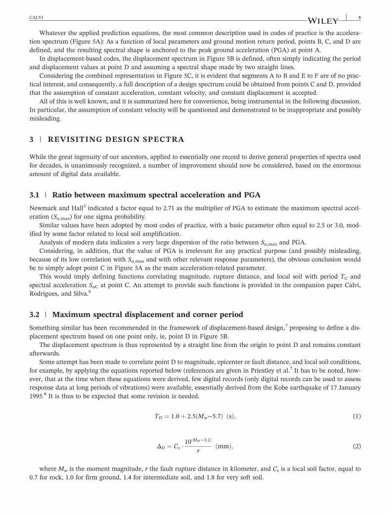
Based on the same data, amplification factors to construct design spectra from peak ground values were recom-mended. As an example, see the design spectrum depicted in Figure 4, again copied from Newmark and Hall,3 basedon a peak ground acceleration equal to 0.5 g, which was asserted to correspond to one sigma cumulative probability,although it is not clear how probability could be treated in presence of so few data.

According to the description of Newmark and Hall,3 and referring to periods rather than frequencies, a designspectrum should show a constant maximum displacement demand at period approximately longer than 3 seconds, aconstant maximum acceleration demand at periods between about 0.15 and 0.5 second and a constant maximum veloc-ity demand between 0.5 and 3 seconds.

FIGURE 2 Typical response spectrum from earthquake motions, as reported in Newmark and Hall.3 Displacements are in inches

(1 in = 25.4 mm). The values indicated with the subscript m are peak ground values. β indicates the damping value (5%)

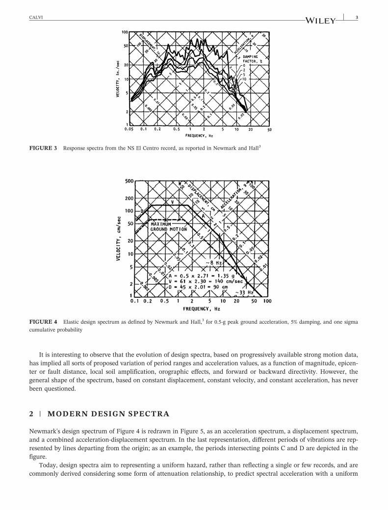
FIGURE 3 Response spectra from the NS El Centro record, as reported in Newmark and Hall3

FIGURE 4 Elastic design spectrum as defined by Newmark and Hall,3 for 0.5‐g peak ground acceleration, 5% damping, and one sigma

cumulative probability

CALVI 3

It is interesting to observe that the evolution of design spectra, based on progressively available strong motion data,has implied all sorts of proposed variation of period ranges and acceleration values, as a function of magnitude, epicen-ter or fault distance, local soil amplification, orographic effects, and forward or backward directivity. However, thegeneral shape of the spectrum, based on constant displacement, constant velocity, and constant acceleration, has neverbeen questioned.

2 | MODERN DESIGN SPECTRA

Newmark's design spectrum of Figure 4 is redrawn in Figure 5, as an acceleration spectrum, a displacement spectrum,and a combined acceleration‐displacement spectrum. In the last representation, different periods of vibrations are rep-resented by lines departing from the origin; as an example, the periods intersecting points C and D are depicted in thefigure.

Today, design spectra aim to representing a uniform hazard, rather than reflecting a single or few records, and arecommonly derived considering some form of attenuation relationship, to predict spectral acceleration with a uniform

(A)

(B)

(C)

FIGURE 5 Newmark's design spectrum of Figure 4, shown as acceleration spectrum A, displacement spectrum B, and combined

acceleration‐displacement spectrum C, [Colour figure can be viewed at wileyonlinelibrary.com]

4 CALVI

probability of exceedance at different period values as a function of source and propagation parameters. The literatureon the subject is endless; as a fundamental historical contribution and a recent summary, see Cornell4 and Mulargia,Stark, and Geller.5

CALVI 5

Whatever the applied prediction equations, the most common description used in codes of practice is the accelera-tion spectrum (Figure 5A): As a function of local parameters and ground motion return period, points B, C, and D aredefined, and the resulting spectral shape is anchored to the peak ground acceleration (PGA) at point A.

In displacement‐based codes, the displacement spectrum in Figure 5B is defined, often simply indicating the periodand displacement values at point D and assuming a spectral shape made by two straight lines.

Considering the combined representation in Figure 5C, it is evident that segments A to B and E to F are of no prac-tical interest, and consequently, a full description of a design spectrum could be obtained from points C and D, providedthat the assumption of constant acceleration, constant velocity, and constant displacement is accepted.

All of this is well known, and it is summarized here for convenience, being instrumental in the following discussion.In particular, the assumption of constant velocity will be questioned and demonstrated to be inappropriate and possiblymisleading.

3 | REVISITING DESIGN SPECTRA

While the great ingenuity of our ancestors, applied to essentially one record to derive general properties of spectra usedfor decades, is unanimously recognized, a number of improvement should now be considered, based on the enormousamount of digital data available.

3.1 | Ratio between maximum spectral acceleration and PGA

Newmark and Hall3 indicated a factor equal to 2.71 as the multiplier of PGA to estimate the maximum spectral accel-eration (Sa,max) for one sigma probability.

Similar values have been adopted by most codes of practice, with a basic parameter often equal to 2.5 or 3.0, mod-ified by some factor related to local soil amplification.

Analysis of modern data indicates a very large dispersion of the ratio between Sa,max and PGA.Considering, in addition, that the value of PGA is irrelevant for any practical purpose (and possibly misleading,

because of its low correlation with Sa,max and with other relevant response parameters), the obvious conclusion wouldbe to simply adopt point C in Figure 5A as the main acceleration‐related parameter.

This would imply defining functions correlating magnitude, rupture distance, and local soil with period TC andspectral acceleration SaC at point C. An attempt to provide such functions is provided in the companion paper Calvi,Rodrigues, and Silva.6

3.2 | Maximum spectral displacement and corner period

Something similar has been recommended in the framework of displacement‐based design,7 proposing to define a dis-placement spectrum based on one point only, ie, point D in Figure 5B.

The displacement spectrum is thus represented by a straight line from the origin to point D and remains constantafterwards.

Some attempt has been made to correlate point D to magnitude, epicenter or fault distance, and local soil conditions,for example, by applying the equations reported below (references are given in Priestley et al.7 It has to be noted, how-ever, that at the time when these equations were derived, few digital records (only digital records can be used to assessresponse data at long periods of vibrations) were available, essentially derived from the Kobe earthquake of 17 January1995.8 It is thus to be expected that some revision is needed.

TD ¼ 1:0þ 2:5 Mw−5:7ð Þ sð Þ; (1)

ΔD ¼ Cs ⋅10 MW−3:2ð Þ

rmmð Þ; (2)

where Mw is the moment magnitude, r the fault rupture distance in kilometer, and Cs is a local soil factor, equal to0.7 for rock, 1.0 for firm ground, 1.4 for intermediate soil, and 1.8 for very soft soil.

6 CALVI

3.3 | Combination of the two horizontal components

When deriving equations of the sort of 1 and 2, a problem rises up immediately. The two recorded horizontal compo-nents of a ground motion have clearly the same magnitude, distance, soil, etc. Unfortunately, they usually show verydifferent values in terms of peak spectral acceleration and displacement, in many cases even mixing the larger demandin acceleration with the smaller displacement and vice versa.

Several solutions are possible, for example, adopting the spectrum resulting from the envelope of the two, orcalculating for each abscissa, an ordinate resulting from the square root of the sum of the squares of the ordinates ofthe two spectra.

This problem has been clearly focused and rigorously faced by Boore, Watson‐Lamprey, and Abrahamson9 andBoore,10 where different components of the signals are calculated (eg, median [ROT50] or maximum [ROT100] ampli-tudes). Here, it is suggested to derive one single horizontal acceleration signal, combining the two components instantby instant. This will imply producing spectra that do not correspond to any specific direction, being actually sort of“rotating” spectra, without any specification of the actual direction for each maximum value (similar to the ROT100proposed by Boore10). The resulting spectrum will be similar to the envelope of the spectral components, being normallydominated by the largest acceleration vector instant by instant, and it seems quite consistent with the concept of designspectrum. It has to be noted that this suggestion has nothing to do with the combination of actions on buildings,resulting from their response in different directions. As discussed by Stewart et al,11 the need to consider the differentresponses in different directions of “azimuth‐dependent” structures remains untouched.

3.4 | Why constant velocity?

As previously discussed, the point of arrival of some 30 years of speculations about the appropriate shape of a designspectrum was to adopt three criteria in different period ranges, ie, constant acceleration at low periods, constant dis-placement at long periods, and constant velocity in an intermediate range.

While the first two indications are based on physical considerations and are essentially shared here, consistentlywith what is discussed in the previous paragraphs, the choice of keeping a constant velocity in the intermediate rangeis only apparently sound, although never thoroughly questioned in the past.

Indeed, the idea of replacing the standard spectral shapes by a “multiperiod” spectral definition has been discussedboth in Europe (eg, within the Project SHARE, http://www.share‐eu.org/), or with reference to the Italian uniform haz-ard map; see Faccioli and Villani12 and in the United States.13 Smerzini, Galasso, Iervolino, and Paolucci14 explicitlysuggested the possibility of modifying the exponent applied to the period T in the equation defining the descendingbranch of the acceleration response spectrum, using values between 0.85 and 1.4 instead of 1. However, consistent withthe declared objective of defining long period spectral ordinates, the corner period of the displacement spectrum wascalculated first, and the exponent was calculated to assure compatibility between the short and long period branchesof the spectrum.

Returning to the construction of the spectra shape operated in the seventies, it can be noted that the constantvelocity assumption is not only biased by the use of a single ground motion, but also by the representation of dataon a logarithmic scale (see Figures 2 and 3; Newmark and Hall3).

As an example, assume to adopt a straight line between points C and D of Figure 5C, as shown in Figure 6. Theresulting design spectrum, plotted in red in Figure 6, shows possible differences of 100% in terms of displacementand acceleration demand in the wide intermediate region that characterizes the vast majority of structures, with fewexceptions, such as isolated buildings or suspension bridges.

However, such major differences are much less evident if the data are plotted adopting a tri‐logarithmic scale, asshown in Figure 7. The variation of about 30% in the peak velocity (from about 140 to about 200 cm/s) does not appearin evident mismatching with the experimental data.

Note that something similar is shown in the conceptual response spectrum of Figure 2, reported from Newmarkand Hall.3

It may be surprising to observe that the constant velocity rule has never been questioned in so many years. This maybe an effect of the great respect we all feel for the researchers who developed the concept of spectra. However, it is alsocurious to note that a trilinear curve like the one discussed perfectly describes the capacity range of a dynamic testingrig. Consider as an example the case of a shaking table:

FIGURE 7 The same spectra shown in Figure 6, drawn on a tri‐logarithmic paper [Colour figure can be viewed at wileyonlinelibrary.com]

FIGURE 6 The Newmark design spectrum compared with a spectrum with no constant velocity region, where Sa varies linearly with Sd in

the intermediate periods region [Colour figure can be viewed at wileyonlinelibrary.com]

CALVI 7

• the maximum acceleration derives from the force capacity (ie, the area of the actuator piston multiplied by the oilpressure) divided by the total mass of table and payload;

• the maximum velocity results from the oil flow capacity divided by the area of the piston;• the maximum displacement is simply one‐half of the stroke of the actuator.

As such, a comparison between a ground motion spectrum and the table capacity will immediately allow to evaluatewhether that ground motion will be reproducible. Unfortunately, this does not mean at all that any ground motion spec-trum should be characterized by a constant velocity range.

The adoption of a linear segment between points C and D should not be intended as a proposal, but rather as a prov-ocation, that may become a proposal only if sustained by appropriate experimental evidence. This is the subject of acompanion paper (Calvi et al,6).

4 | EL CENTRO RESPONSE SPECTRA

As repeatedly mentioned, the ground motions recorded at El Centro on 18 May 1940, and namely, the NS component(Figure 3), have been the main reference until the eighties. Both spectra (NS and EW) are plotted in Figure 8, using the

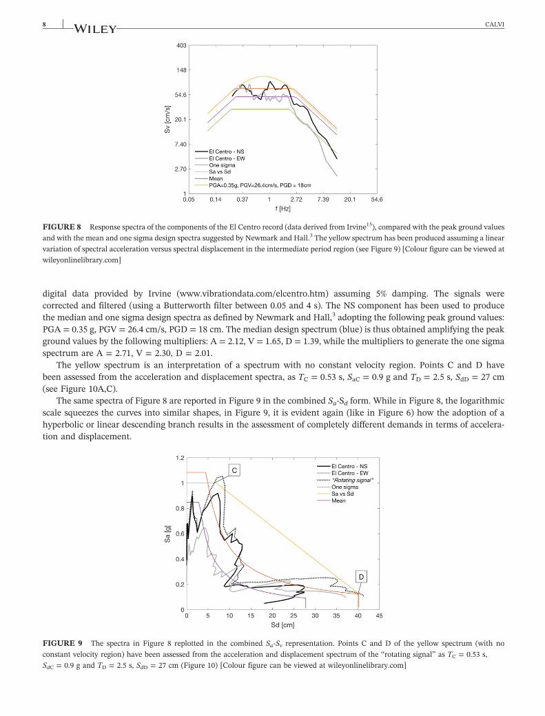
FIGURE 8 Response spectra of the components of the El Centro record (data derived from Irvine15), compared with the peak ground values

and with the mean and one sigma design spectra suggested by Newmark and Hall.3 The yellow spectrum has been produced assuming a linear

variation of spectral acceleration versus spectral displacement in the intermediate period region (see Figure 9) [Colour figure can be viewed at

wileyonlinelibrary.com]

8 CALVI

digital data provided by Irvine (www.vibrationdata.com/elcentro.htm) assuming 5% damping. The signals werecorrected and filtered (using a Butterworth filter between 0.05 and 4 s). The NS component has been used to producethe median and one sigma design spectra as defined by Newmark and Hall,3 adopting the following peak ground values:PGA = 0.35 g, PGV = 26.4 cm/s, PGD = 18 cm. The median design spectrum (blue) is thus obtained amplifying the peakground values by the following multipliers: A = 2.12, V = 1.65, D = 1.39, while the multipliers to generate the one sigmaspectrum are A = 2.71, V = 2.30, D = 2.01.

The yellow spectrum is an interpretation of a spectrum with no constant velocity region. Points C and D havebeen assessed from the acceleration and displacement spectra, as TC = 0.53 s, SaC = 0.9 g and TD = 2.5 s, SdD = 27 cm(see Figure 10A,C).

The same spectra of Figure 8 are reported in Figure 9 in the combined Sa‐Sd form. While in Figure 8, the logarithmicscale squeezes the curves into similar shapes, in Figure 9, it is evident again (like in Figure 6) how the adoption of ahyperbolic or linear descending branch results in the assessment of completely different demands in terms of accelera-tion and displacement.

FIGURE 9 The spectra in Figure 8 replotted in the combined Sa‐Sv representation. Points C and D of the yellow spectrum (with no

constant velocity region) have been assessed from the acceleration and displacement spectrum of the “rotating signal” as TC = 0.53 s,

SdC = 0.9 g and TD = 2.5 s, SdD = 27 cm (Figure 10) [Colour figure can be viewed at wileyonlinelibrary.com]

(A)

(B)

(C)

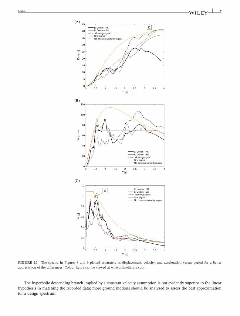
FIGURE 10 The spectra in Figures 8 and 9 plotted separately as displacement, velocity, and acceleration versus period for a better

appreciation of the differences [Colour figure can be viewed at wileyonlinelibrary.com]

CALVI 9

The hyperbolic descending branch implied by a constant velocity assumption is not evidently superior to the linearhypothesis in matching the recorded data; more ground motions should be analyzed to assess the best approximationfor a design spectrum.

10 CALVI

It has to be noted that in the seventies, a lot of ingenuity was applied to provide suggestions to define design spectraat low frequencies (or long periods: There is little evidence of anything at periods longer than 4 s in the responsespectrum).

The same spectra of Figures 8 and 9 are plotted singularly as acceleration, velocity, and displacement versus periodin Figure 10. In these representations, too, it seems difficult to state which one of the design spectra in orange or redbetter matches the El Centro response spectra.

In Figures 9 and 10, the spectra resulting from an accelerogram generated by the vectorial combination, instant byinstant, of the NS and ES acceleration components are also reported. These spectra differ significantly from thoseobtained from the NS component only at long periods of vibration, where the displacement demand is larger and theEW component seems to be dominant.

The design spectrum suggested by Newmark and Hall3 seems to take into consideration the displacement demand ofthe ES component, even if this was not explicitly stated. This extended use of common sense and intelligence is the baseof the longevity of the spectral shape defined in the central decades of the previous century.

5 | DEALING WITH NON ‐LINEAR RESPONSE

As thoroughly described by Riddell,16 the first attempts to determine the maximum response of nonlinear systems bymeans of inelastic response spectrum, date back to the fifties. Reference will be made again to the summary ofNewmark and Hall3 to comment on appropriate choices and present needs.

The basic idea to derive inelastic spectra from their elastic counterpart was based on defining ranges of the spectrumwhere acceleration, velocity, and displacement were assumed to be “conserved” or modified by some correction factor.The key figure reported by Newmark and Hall3 is reproduced as Figure 11. Here, an elastic‐perfectly‐plastic system isassumed, characterized by a ratio between displacement capacity and yield displacement equal to the displacementductility value μ. Under these assumptions, the rules applied to derive inelastic spectra were the following:

• Divide the ordinate of the elastic spectrum by μ for frequencies up to about 2 Hz (regions D and V in Figure 6) toobtain the acceleration inelastic spectrum.

• Do the same in the frequency range between 2 and 8 Hz (region A), dividing by (2 μ−1)0.5 instead of μ.• Keep the same acceleration in the elastic and inelastic spectrum for frequencies higher than 33 Hz.• Link linearly the ordinates at 8 and 33 Hz in the logarithmic plot.• To obtain the inelastic displacement spectrum, multiply all the ordinates of the inelastic acceleration spectrum by μ.

This approach has been discussed, corrected, and modified in minor aspects for decades but essentially used in itsbasic structure in all force‐based approaches (and as such in all codes of practice) until today.

The procedure is different if a displacement‐based approach is applied (Priestley et al7). In this case, it is suggested totake into consideration a correction of the spectral shape only due to the energy dissipated in the hysteretic cycles and to

FIGURE 11 Derivation of acceleration and displacement inelastic spectra from an elastic spectrum (Newmark and Hall3 and Riddell15)

CALVI 11

use an elastic equivalent system with a stiffness (and thus a period) secant to the intersection between design displace-ment and corrected displacement spectrum.

Design equations are detailed by Priestley et al,7 and this is not the place to discuss again the procedure.However, to have a feeling of these different approaches, a comparison is provided in Figure 12, where all spectra

have been redrawn in a combined spectral acceleration versus spectral displacement form. An inelastic system withan initial period of vibration of about 0.5 second and a ductility μ = 3 is designed according to Newmark and Hall,3

obtaining a design acceleration of about 0.6 g and a corresponding displacement of about 18 cm. A similar system wouldprobably be designed for a displacement of about 30 cm according to Priestley et al,7 assessing a displacement reductionfactor (its meaning is discussed in the following section) of about 0.64. The resulting design acceleration would be about0.28 g, less than one‐half with respect to the previous case.

Both expected nonlinear responses (the orange and green curves in Figure 12) seem compatible with the demandrepresented by the blue spectrum, derived from the elastic spectrum applying a factor to account for equivalent dampingonly. As such, they look more like different design options than like a correct and a wrong solution, but note thatadopting a linear spectral shape (light blue in the figure), the two approaches would lead to similar expected responses(dashed yellow and black arrows).

This result is just a simple example and should not be generalized; actually, as discussed by Priestley et al7 and byPriestley,17 the required strength resulting from a displacement‐based approach can be higher or lower with respect tothat resulting from a traditional force‐based approach. The result depends on the characteristics of the structural systembut as well on the site seismicity, since a displacement‐based approach induces more dramatic variations in the requiredstrength.

6 | CORRECTION OF THE ELASTIC DESIGN SPECTRUM TO ACCOUNT FORENERGY DISSIPATION

Today, it is indisputably accepted that demand and capacity should be kept as much as possible on different sides of aninequality and that the nonlinear response should be captured as much as possible on the capacity side.

This can be accomplished using various forms of pushover analysis and applying one of the methods derived to com-pare demand and capacity. One option is to apply a formulation of the capacity spectrum method, originally proposedby Freeman,18 a second one is to resort to the N2 method, originally proposed by Fajfar and Fishinger19 and currently

FIGURE 12 Playing with Newmark design spectrum: in dashed black the elastic spectrum; in grey, the acceleration and displacement

inelastic spectra according to Newmark and Hall3; in dashed red, the spectral design acceleration and displacement of a system with a

period of approximately 0.5 seconds; in orange, a possible capacity curve representing the nonlinear response of this system; in blue, the

inelastic spectrum according to Priestley et al7 (lighter blue: modification according to Figure 6); in black, the spectral design acceleration for

the same system, designed for a displacement of about 30 cm; in green, a possible capacity curve representing the nonlinear response of this

last system; in dotted orange, the expected design change of the first system, with a modified spectral shape; in dotted black, the expected

design change of the second system, with a modified spectral shape [Colour figure can be viewed at wileyonlinelibrary.com]

12 CALVI

recommended by EC8. A further possibility is to consider linear equivalent approaches as discussed by Priestley et al7

but originally proposed by Shibata and Sozen.20 A detailed discussion of this subject falls outside the scope of thispaper; the interested reader is addressed to the critical summary provided by Pinho, Marques, Monteiro, Casarotti,and Delgado.21

Considering instead the side of demand, it is still preferred to correct the elastic spectra to account for energy dissi-pation rather than modifying the capacity curve. This can be accomplished by applying to the displacement spectrumordinates a “displacement reduction factor” ηξ as a function of an “equivalent hysteretic damping” ξh (Priestleyet al7), estimated by some energy equivalence (Jacobsen22). While several formulations are available, consider as anexample the equations recommended by Priestley et al7:

ηξ ¼0:07

0:02þ ξ

� �0:5

; (3)

ξ ¼ ξ0 þ ξh ¼ ξ0 þ Cμ−12πμ

� �; (4)

where ξ is the total equivalent damping of the system, ξ0 is the inherent damping (usually taken as 0.05), C is a func-tion of the shape of the hysteresis loop (generally in the range of 0.3‐0.6), and μ is the ductility of the system.

An open problem is an appropriate tuning of η, expressed as a function of magnitude, source‐to‐site distance, siteconditions, faulting style etc (eg, Priestley et al7 recommended to reduce the exponent from 0.5 to 0.25 in case of nearfield ground motion) but possibly of other parameters. For example, based on analyses of specific Turkish groundmotions, Akkar and Kale23 recommend to reduce η with period elongation. The resulting reduced spectra are depictedin Figure 13, considering the design spectrum of Figure 6. It is again evident that a different shape of the “constantvelocity” branch will have significant effects on demand (likely, more than the correction based on period of vibration).

A reformulation of design spectra will pave the way for consequent revisitations of nonlinear floor spectra, whichare the most viable tool to design nonstructural elements and are today treated by most codes of practice in an improperway, as thoroughly discussed by Calvi24 and Calvi and Sullivan.25

7 | CONCEPTUAL PROPOSAL TO GENERATE DESIGN SPECTRA

As previously discussed, it is suggested that the design spectra corresponding to a given set of ground motions (consis-tent with the assumed magnitude and rupture distance) will be first defined as a function of two points, identified as thelongest period (TC) at which the spectral acceleration will be at the peak amplification (SaC) and the shortest period (TD)at which the spectral displacement will reach its maximum value (SdD).

FIGURE 13 The design spectra of Figure 6 reduced applying a displacement reduction factor based on Equation 3 and the correction

suggested by Akkar and Kale at increasing period of vibration [Colour figure can be viewed at wileyonlinelibrary.com]

CALVI 13

These four values will be set as a function of magnitude, distance, local amplification, or whatever else will emergefrom the analysis of recorded ground motions.

In the intermediate region, it is felt appropriate to apply a function of a single parameter, able to connect point(SdC; SaC) and point (SdD; SaD) with a shape that may vary for different magnitude and different distance from theepicenter. Such an equation has been derived in analogy to the function that allow to modify the shape of a force‐displacement curve of a viscous damper, ie, considering the combination of two sinusoidal functions, as follows:

y ¼ sinαt; (5)

z ¼ cosαt; (6)

y ¼ sinα cos−1 z1=α� �� �

: (7)

Varying α, this equation can take any form between points (0; 1) and (1; 0), as shown in Figure 14.Applying a coordinate transformation, from point (0; 1) to point (SdC; SaC) and from point (1; 0) to point (SdD; SaD),

the following equation is derived:

Sa ¼ SaD þ SaC−SaD� �

⋅ sinα cos−1Sd−SdCSdD−SdC

� �1α

!: (8)

Note that in Equation 8, two derived parameters are used, as follows:

SdC ¼ SaCT2C

4π2; (9)

SaD ¼ SdD4π2

T2D

: (10)

As anticipated, Equation 8, which may look complex but it is actually easy to implement and only depends on oneparameter (α), allows defining a family of curves that can reproduce any shape in the spectral acceleration versusspectral displacement curve, as shown, for example, in Figure 15.

In that figure, the two critical points have been set as TC = 0.53 s, SaC = 0.9 g and TD = 2.5 s, SdD = 27 cm. Thesevalues are the same used in Figures 8, 9, and 10 with reference to the El Centro ground motion.

FIGURE 14 Graphical expression of Equation 7 [Colour figure can be viewed at wileyonlinelibrary.com]

FIGURE 15 Design spectra created applying Equation 5 and assuming the following parameters: TC = 0.53 s, SaC = 0.9 g, TD = 2.5 s,

SdD = 27 cm [Colour figure can be viewed at wileyonlinelibrary.com]

14 CALVI

The three shapes of the intermediate region shown in Figure 15 corresponds to α = 1 (green), α = 2 (red, in whichcase, the curve reduced to a straight line), and α = 3 (blue).

While the differences in the acceleration, displacement, and velocity spectra may not appear so relevant, it is evidentin the combined Sa vs Sd spectrum that a proper selection of α may result in completely different design or assessmentpoints.

A discussion of proper values to be adopted for α as a function of magnitude and distance is presented in thecompanion paper (Calvi et al,6).

8 | CONCLUSIONS

Evidently, this is an opinion paper, and the conclusions have the same flavor and meaning. Derivation and tuning ofequations based on actual data, validation, and verification are the subject of the companion paper (Calvi et al,6) andof future research studies.

8.1 | Definition of elastic design spectra

It is suggested that peak ground acceleration should be abandoned as a key parameter of demand and hazard. Spectralshape and “anchor” should be based on the definition of two points (C and D in this paper—see Figure 9), ie, maximumspectral acceleration and displacement with the corresponding periods of vibration.

The spectra shape in the intermediate region, roughly ranging from 0.5 to 3 seconds, should be investigated anddefined, abandoning the concept of constant velocity, which has no theoretical nor experimental base. An equationto define the shape of the intermediate region as a function of a single parameter (α, Equation 5) is proposed, on thebase of speculation only.

Points and shape should be possibly defined as a function of magnitude, distance from epicenter or fault, sourcemechanism, expected duration or number of significant cycles, and soil type. Other factors may be considered but arenot evidently relevant.

CALVI 15

Design spectra should be instrumental to design and as such not necessarily derived as a weighted combination oran average of response spectra.

Parts of design spectra where displacement or acceleration demand is varying rapidly should be avoided, since theymay not be justified from a probability point of view and may result in sources of potential risk.

8.2 | Effects of spectra shapes on design

With reference to the discussion associated to Figure 12, it appears that the definition of strength and displacementcapacity to be attained in structural design has been a rather casual business. Actually, it is evident that differencesof 100% may have easily arisen, and one may consequently wonder whether is there dependability in the results andin the constructed environment.

The answer is twofold: On one side, there are enormous differences in the risk associated to different structures,even if they all might be above a certain threshold; on the other side, it may be concluded that resilience is the mostrelevant property to be assured to any construction, and therefore, the most effective solution is a strict application ofcapacity design rules.

It is curious to note that even performing full nonlinear time history analyses does not help in favoring a uniformrisk level, since the input ground motions are derived from possibly biased design spectra or at least are smoothedand corrected in the expected response region to assure uniformity to design spectra.

8.3 | Combination of the two horizontal components

For validation and tuning purposes, it is suggested to derive one single horizontal acceleration signal from recordedground motions, combining the two components instant by instant. The resulting signal, and consequently the corre-sponding generated spectrum, will be “rotating,” indicating in each instant the magnitude of the demand vector. Thisapproach seems quite consistent with the spectrum concept and will allow to define single values for point C and Dfor each ground motion (a more rigorous discussion of this point is presented by Boore10).

The definition of such single spectrum has nothing to do with the combination of actions on buildings, resultingfrom their response in different directions (Stewart et al11).

8.4 | Accounting for structural response

Although accepted to keep as separated as possible demand and capacity, the effect of energy dissipation in structuralresponse is still best included on the demand side, in the form of a correction factor in the response spectra.

It has to be positively considered that the correction factor due to energy dissipation should not be smaller than 0.5,with a consequent relatively low sensitivity to estimation errors.

However, a finer tuning of this reduction factor, possibly considering source mechanism, period of vibration andexpected ground motion duration, or number of significant cycles is desirable.

The proper anchoring of spectra and the combination rules for different load cases and directions should be tunedconsidering the protection factors embedded in codes, with reference to some accepted probability of attaining specificlimit states.

8.5 | Hazard maps and data

Basic hazard maps are still drawn as a function of peak ground acceleration, although recent hazard studies have pro-vided results in terms of acceleration spectral ordinates.

As pointed out, the use of PGA as a reference parameter may be a source of errors, wrong beliefs, and misinterpre-tations. In case of needing a single parameters, it is suggested to use a spectral ordinate, namely, the accelerationdemand at point C or, better, the displacement demand at point D.

As stated, modern hazard maps are associated to a bevy of data, which may include several spectral ordinates orentire response spectra for different annual probability of exceedance. These response spectra may again become apotential source of mistakes and misinterpretations. Being the product of probabilistic seismic hazard assessment stud-ies, resulting from weighted combinations of different source mechanisms and ground motion prediction equations,they should rather be regarded as some sort of average response spectra than as design spectra.

16 CALVI

In particular, design spectra should somehow consider the inherent variability on the side of capacity and avoid asmuch as possible situations in which small variations in the assessed strength or displacement capacity or equivalentperiod of vibration would lead to relevant modifications of the corresponding demand.

8.6 | Validation and tuning

As repeatedly stated, the significance and validity of this opinion paper will only be assessed by proper comparisonswith recorded data and consequently by its capacity of inspiring new, simple, laws able to interpret empirical data.

A patient work of validation and tuning is thus needed.A first series of results, related to 360 recorded ground motions recorded in Italy between 1972 and 2017, is pre-

sented in the companion paper (Calvi et al,6).

8.7 | El Centro ground motion, Imperial Valley earthquake, 18 May 1940

One final philosophical question remains, beyond the ingenuity of those who created sound design response spectrafrom a single ground motion component and possibly beyond the analysis of recent Italian data: how should the ElCentro ground motion be interpreted: a fortunate unicorn or the ancestral ape of all possible ground motions?

ACKNOWLEDGMENTS

The work presented in this paper has been developed within the framework of the project “Dipartimenti di Eccellenza,”funded by the Italian Ministry of Education, University and Research at IUSS Pavia.

ORCID

Gian Michele Calvi http://orcid.org/0000-0002-0998-8882

REFERENCES

1. Chopra AK. Elastic response spectrum: A historical note. Earthquake Engineering and Structural Dynamics. 2007;36(1):3‐12.

2. Housner GW. Calculating response of an oscillator to arbitrary ground motion. Bulleting of the Seismological Society of America.1941;31:143‐149.

3. Newmark NM, Hall WJ. Earthquake spectra and design. Oakland, CA: Engineering Monographs, EERI; 1982.

4. Cornell CA. Engineering seismic hazard analysis. Bull Seismol Soc Am. 1968;59(5):1583‐1606.

5. Mulargia F, Stark PB, Geller RJ. Why is probabilistic seismic hazard (PSHA) analysis still used? Physics of the Earth and Planetary Interior.2017;264:63‐75.

6. Calvi, G.M., D. Rodrigues and V. Silva (2018). Response and design spectra from Italian earthquakes 2012‐2017. Companion Paper, thisJournal

7. Priestley MJN, Calvi GM, Kowalsky MJ. Displacement based seismic design of structures. Pavia: IUSS Press; 2007.

8. Tolis SV, Faccioli F. Displacement design spectra. Journal of Earthquake Engineering. 1999;3(1):107‐125.

9. Boore DM, Watson‐Lamprey J, Abrahamson NA. Orientation‐independent measures of ground motion. Bull Seismol Soc Am.2006;96(4):1502‐1511.

10. Boore DM. Orientation‐independent, nongeometric‐mean measures of seismic intensity from two horizontal components of motion. BullSeismol Soc Am. 2010;100(4):1830‐1835.

11. Stewart JP, Abrahansom NA, Atkinson GM, et al. Representation of bidirectional ground motions for design spectra in building codes.Earthq Spectra. 2011;27(3):927‐937.

12. Faccioli E, Villani M. Seismic hazard mapping for Italy in terms of broadband displacement response spectra. Earthq Spectra.2009;25(3):515‐539.

13. Hamburger R., N. Luco, M. Tong and P. Schneider (2017). Recommendations of Project'17 planning committee. Paper n. 4608, Proc. of the16th WCEE Santiago, Chile

14. Smerzini C, Galasso C, Iervolino I, Paolucci R. Ground motion record selection based on broadband spectral compatibility. EarthqSpectra. 2014;30(4):1427‐1448.

CALVI 17

15. Irvine, T. http://www.vibrationdata.com/elcentro.htm, Vibrationdata, Madison, AL

16. Riddell R. Inelastic response spectrum: Early history. Earthquake Engineering and Structural Dynamics. 2008;37(8):1175‐1183.

17. Priestley MJN. Myths and fallacies in earthquake engineering, re‐visited. Pavia: IUSS Press; 2003.

18. Freeman, S. A. (1975). Evaluation of existing buildings for seismic risk: A case study of Puget Sound Naval Shipyard, Bremerton,Washington. Proceedings of the 1st US Nat. Conf. on Earthquake Engineering, EERI, Oakland, CA, 133–122

19. Fajfar, P. and M. Fishinger (1988). N2—A method for nonlinear analysis of regular buildings. Proceedings of the 9th WCEE, Tokyo andKyoto, vol. V, 111–116

20. Shibata A, Sozen M. Substitute structure method for seismic design in reinforced concrete. ASCE Journal of Structural Engineering.1976;102(1):1‐18.

21. Pinho R, Marques M, Monteiro R, Casarotti C, Delgado R. Evaluation of nonlinear static procedures in the assessment of building frames.Earthq Spectra. 2013;29(4):1459‐1476.

22. Jacobsen, L.S. (1960). Damping in composite structures. Proceedings of the 2nd WCEE, Tokyo and Kyoto, vol. II, 1029–1044

23. Akkar, S. and O. Kale (2015). Revised probabilistic hazard map of Turkey and its implications on seismic design. EU Workshop“Elaboration of Maps for Climatic and Seismic Actions for Structural Design in the Balkan region”, Zagreb

24. Calvi PM. Relative displacement floor spectra for seismic design of non‐structural elements. Journal of Earthquake Engineering.2014;18(7):1037‐1059.

25. Calvi PM, Sullivan TJ. Estimating floor spectra in multiple degree of freedom structures. Earthquake and Structures. 2014;7(1):17‐38.

How to cite this article: Calvi GM. Revisiting design earthquake spectra. Earthquake Engng Struct Dyn.2018;1–17. https://doi.org/10.1002/eqe.3101