Revision 00 of ANL-EBS-MD-000036, 'Incorporation of ... · MANAGEMENT ANALYSIS/MODEL REVISION...

DISCLAIMER

This contractor document was prepared for the U.S. Department of Energy (DOE), but has not

undergone programmatic, policy, or publication review, and is provided for information only.

The document provides preliminary information that may change based on new information or

analysis, and represents a conservative treatment of parameters and assumptions to be used

specifically for Total System Performance Assessment analyses. The document is a preliminary

lower level contractor document and is not intended for publication or wide distribution.

Although this document has undergone technical reviews at the contractor organization, it has not

undergone a DOE policy review. Therefore, the views and opinions of authors expressed may

not state or reflect those of the DOE. However, in the interest of the rapid transfer of

information, we are providing this document for your information per your request.

OFFICE OF CIVILIAN RADIOACTIVE WASTE MANAGEMENT 1. QA: QA

ANALYSIS/MODEL COVER SHEET eage: 1 " of: so

Complete Only Applicable Items

2. M Analysis Check all that apply 3. R Model Check all that apply

Type of [ Engineering Type of El Conceptual Model El Abstraction Model Analysis Model

A y Performance Assessment El Mathematical Model El System Model

E_ Scientific El Process Model

Intended Use El Input to Calculation Intended El Input to Calculation of Analysis Use of

El Input to another Analysis or Model Model [] Input to another Model or Analysis

El Input to Technical Document El Input to Technical Document

El Input to other Technical Products El Input to other Technical Products

Describe use: Describe use:

This analysis provides conceptual input for the treatment of uncertainty and variability in waste package degradation

4. Title:

Incorporation of Uncertainty and Variability of Drip Shield and Waste Package Degradation in WAPDEG Analysis

5. Document Identifier (including Rev. No. and Change No., if applicable):

ANL-EBS-MD-000036 REV 00

6. Total Attachments: 7. Attachment Numbers - No. of Pages in Each:

N/A 1_N1_4

Printed Name Signature Date

8. Originator Jon C. Helton - /

9. Checker Bryan E. Bullard lax

10. Lead/Supervisor Joon H. Lee

11. Responsible Manager Robert J. MacKinnon

12. Remarks: /

Initial issue.

Per Section 5.5.6 of AP-3.10Q, the responsible manager has determined that the subject AMR is not subject to AP-2.14Q review because

the analysis does not affect a discipline or area other than the originating organization (Performance Assessment). The downstream user

of the information resulting from this AMR is the Performance Assessment (PA) Dept., which is also the originating organization of this

work. There are no upstream input feeds to this AMR from other organizations. Furthermore, the subject AMR does not provide any input

feeds to the TSPA-SR and only provides a technical basis for a better conceptual understanding of how uncertainty and variability can be

treated in waste package degradation modeling. Therefore, no formal AP-2.14Q reviews were requested or determined to be necessary.

INFORMATION =COPY

;LAS VE:GAS DMOCUMENT CCONNTROLL

Enclosure 12 �ev. 02/25/2000

AP-3.1 0Q.4 Enclosure 12 lev. 02/25/2000

OFFICE OF CIVILIAN RADIOACTIVE WASTE MANAGEMENT

ANALYSIS/MODEL REVISION RECORD Complete Only Applicable Items 1. Page: 2 of: 50

2. Analysis or Model Title:

Incorporation of Uncertainty and Variability of Drip Shield and Waste Package Degradation in WAPDEG Analysis

3. Document Identifier (including Rev. No. and Change No., if applicable):


4. Revision/Change No. 5. Description of Revision/Change __

REV 00 Initial issue.

1.

Rev. 02/25/2000AP-3.10OQ.4

CONTENTS Page

1. PURPOSE ................................................................................................................................. 5

2. QUALITY ASSURANCE ................................................................................................. 5

3. COMPUTER SOFTW ARE AND M ODEL USAGE ......................................................... 5

4. INPUTS .................................................................................................................................... 5

4.1 DATA AND PARAMETERS ......................................... 6

4.2 CRITERIA ........................................................................................................................ 6

4.3 CODES AND STANDARDS ...................................................................................... 6

5. ASSUMPTIONS ...................................................................................................................... 6

6. ANALYSES ............................................................................................................................. 7

6.1 UNCERTAINTY AND VARIABILITY .................................................................... 7

6.1.1 Intuitive Description ........................................................................................... 7

6.1.2 Historical Perspective (adapted in part from Helton and Burmaster 1996) ..... 8

6.1.3 Hypothetical Corrosion M odel ........................................................................ 12

6.2 ILLUSTRATION OF VARIABILITY AND UNCERTAINTY WITH

HYPOTHETICAL M ODEL ....................................................................................... 16

6.2.1 Single Patch ..................................................................................................... 16

6.2.1.1 Effects of Variability ...................................................................... 16

6.2.1.2 Effects of Variability and Uncertainty ........................................... 18

6.2.2 Single W aste Package ....................................................................................... 19



6.2.3 M ultiple W aste Packages ................................................................................ 22



6.2.4 M ultiple W aste Package Groups .................................................................... 23



6.2.5 M ultiple Patch Types ...................................................................................... 26

6.3 COM PUTATIONAL STRATEGY ........................................................................... 26

6.3.1 Context ................................................................................................................. 26

6.3.2 No Uncertainty in Corrosion Model or Definition of Probability Space

(S', S,, Pv) ........................................................................................................ 28

6.3.3 Uncertainty in Corrosion Model or Definition of Probability Space

(S , S, PV) ............................................................................................................. 30

6.4 MULTIPLE LAYERS: DRIP SHIELD, ALLOY 22, STAINLESS STEEL ........... 31

6.5 UNCERTAINTY IN THE CHARACTERIZATION OF VARIABILITY ................ 31

6.6 GAUSSIAN VARIANCE PARTITIONING ............................................................. 32

ANL-EBS-MD-000036 REV 00 3 of 50 April 2000

7. C O N C LU SIO N S ............................................................................... ! ................................... 42

8. R EFER E N C E S ...................................................................................................................... 44

8.1 DOCUM ENTS CITED ............................................................................................. 44

8.2 CODES, STANDARDS, REGULATIONS, AND PROCEDURES ........................ 49

FIGURES Page

1. Estimate of Probability that Failure Time tf for a Single, Randomly Selected Patch

W ill Be Less Than or Equal to Time t. .............................................................................. 34

2. Estimates of Probability that Failure Time tj for a Single, Randomly Selected Patch

Will Be Less Than or Equal to Time t: (Upper) nR = 100 patches per sample, and

(Lower) nR = 1000 patches per sample ............................................................................... 35

3. Estimates of Probability That Failure Time tf for a Single, Randomly Selected

Patch Will Be Less Than or Equal to Time t: (Upper) Individual Values forprob(tf

< t I xuj),j = 1,2,..., nS, and (Lower) estimated mean and quantile curves for prob(tf

-t xu). 36

4. Example Number of Failed Patches on a Single Waste Package as a Function of

Time: (Upper) nP = 100 patches, and (Lower) nP = 1000 patches ................................ 37

5. Example of Cumulative Distribution Function (CDF) for Time of Initial Waste

Package Failure: (Upper) nP = 100 patches and (Lower) nP = 1000 patches ...................... 38

6. Example of Cumulative Distribution Function (CDF) for Time of Initial Waste

Package Failure: (Upper) nP = 100 patches and (Lower) nP = 1000 patches ................. 39

7. Example of Expected Number of Failed Patches on a Single Waste Package

Divided into nP = 100 Patches as a Function of Time: (Upper) Individual Values

for E(i I t, nP = 100, Xuj),j = 1,2,..., nS (see Equation (24)), and (Lower) Mean and

Quantile Curves for E(i I tnP = 100, xu .)........................................................................ 40

8. Example of Cumulative Distribution Functions (CDFs) for Time of Initial Waste

Package Failure, ti: (Upper) nP = 100 patches, and (Lower) nP = 1000 patches ............ 41

April 2000ANL-EBS-MD-000036 REV 00 4 of 50

1. PURPOSE

This presentation investigates the incorporation of uncertainty and variability of drip shield and

waste package degradation in analyses with the Waste Package Degradation (WAPDEG)

program (CRWMS M&O 1998). This plan was developed in accordance with Development

Plan TDP-EBS-MD-000020 (CRWMS M&O 1999a). Topics considered include (i) the nature of

uncertainty and variability (Section 6.1), (ii) incorporation of variability and uncertainty into

analyses involving individual patches, waste packages, groups of waste packages, and the entire

repository (Section 6.2), (iii) computational strategies (Section 6.3), (iv) incorporation of

multiple waste package layers (i.e., drip shield, Alloy 22, and stainless steel) into an analysis

(Section 6.4), (v) uncertainty in the characterization of variability (Section 6.5), and

(vi) Gaussian variance partitioning (Section 6.6). The presentation ends with a brief concluding

discussion (Section 7).

2. QUALITY ASSURANCE

This analysis was prepared in accordance with the Civilian Radioactive Waste Management

system (CRWMS) Management and Operating Contractor (M&O) Quality Assurance (QA)

program. The information provided in this analysis will be used for evaluating the post-closure

performance of the Monitored Geologic Repository (MGR) waste package and engineered

barrier segment. The Performance Assessment Operations (PAO) responsible manager has

evaluated the technical document development activity in accordance with QAP-2-0, Conduct of

Activities. The QAP-2-0 activity evaluation has determined that the preparation and review of

this technical document is subject to Quality Assurance Requirements and Description (DOE

2000) requirements. In accordance with AP-2.13Q, Technical Product Development Plan, a

work plan was developed, issued, and utilized in the preparation of this document (CRWMS

M&O 1999a). The documentation of this analysis is in accordance with the guidance given in

AP-3.1Q, Conduct of Performance Assessment, and the directions found in AP-3.10Q, Analyses

and Models. There is no determination of importance evaluation developed in accordance with

NLP-2-0, Determination of Importance Evaluations, since the analysis does not involve any field

activity.

3. COMPUTER SOFTWARE AND MODEL USAGE

This presentation involves the discussion of ideas and contains no data analyses in the usual

sense of the word. All figures in Section 6 are for illustration of ideas only. The presentation

used Visual Basic Version 3.0 software for graphing and visual display only, which is exempt

from any AP-SI.1Q qualification requirements.

No models were used or developed in the preparation of this AMR.

4. INPUTS

This presentation involves the discussion of ideas and uses no input data. All results are

hypothetical and are presented for illustration purposes only. See Section 6.

ANL-EBS-MD-000036 REV 00 April 20005 of 50

4.1 DATA AND PARAMETERS

NXA. This presentation involves the discussion of ideas and uses no input data. All results are

hypothetical and are presented for illustration purposes only. See Section 6.

4.2 CRITERIA

N\A. There are no known criteria that are directly applicable to the subject of this analysis.

4.3 CODES AND STANDARDS

NXA. There are no known codes or standards that are directly applicable to the subject of this

analysis.

5. ASSUMPTIONS

This presentation involves the discussion of ideas and contains no data analyses in the usual

sense of the word. All results are hypothetical and are presented for illustration purposes only.

The output of this AMR has no effect on repository performance, therefore, none of the

following assumptions require verification prior to the use of the ideas developed in this

document.

5.1 Corrosion parameters are variable quantities, with variation in their values arising from

small-scale variations in physical and chemical conditions. Computationally simulating

small areas of homogeneous condition referred to as patches represents this variation. It is

assumed that patches are independent and identically distributed for generating-samples for

simulation. This assumption is used throughout this analysis.

5.2 It is assumed that a distinction may be maintained in the corrosion models between

uncertainty and variability each characterized by its own probability space. This

assumption is used throughout this analysis.

5.3 It is assumed that a simulation result CDF will converge to the true CDF as the number of

simulations increase. This assumption is used throughout this analysis.

5.4 Computationally, waste packages are represented as a collection of patches. It is assumed

that the number of patches used is appropriate to represent the variability accurately. It is

assumed that all the patches on a waste package share a common probability space. This

assumption is used throughout this analysis.

5.5 It is assumed that waste packages may be partitioned into groups that share a common

probability space for uncertainty and variability. This assumption is used throughout this

analysis.

A................. of 50 April 2000ANL-EBS-MD-0U03t) RE V 00

6. ANALYSIS

6.1 UNCERTAINTY AND VARIABILITY

6.1.1 Intuitive Description

Two types of inexactness are often present in analyses of complex systems. The first type of

inexactness arises from the consideration of a population in which the individual members have

different properties. This type of inexactness is often referred to as variability. The basic idea

underlying the concept of variability is that a number of possibilities exist that have a real chance

of occurring. Examples of variability include the universe of all possible seven-day sequences of

operating experience at a nuclear power station, the universe of all possible weather conditions

that could occur at a particular location on a specified date, and the universe of all possible

sequences of climatic and geologic events that could occur at the Yucca Mountain site over the

next 10,000 yrs. The designations irreducible, stochastic, aleatory and type A are often used in

reference to what is being referred to as variability in this discussion. In the documentation for

WAPDEG, variability is used in reference to the universe of small-scale corrosion conditions

associated with the waste packages in the repository.

The second type of inexactness arises from a lack of knowledge about a quantity that is believed

to have a fixed value. Thus, the quantity is not variable in the sense used in the preceding

paragraph. Rather, there is a lack of knowledge about what its value should be. In practice, the

quantity in question is often an input to a specific model or analysis, with this model or analysis

having been developed to use a single value for this quantity. This type of inexactn-ess is often

referred to as Uncertainty. The basic idea underlying the concept of uncertainty is lack of

knowledge about a quantity that has a fixed value. Often this quantity is an expected value

calculated over temporal or spatial variability and used as input to a model (e.g., a permeability

used in modeling fluid flow through a geologic formation). The statement that the quantity has a

fixed value is conditional on its use in the model or analysis under consideration. The

designations reducible, subjective, epistemic, state of knowledge, and type B are often used in

reference to what is being referred to as uncertainty in this discussion.

The concepts of variability and uncertainty have been widely discussed in the performance

assessment and risk-assessment communities (see Helton 1997, Helton and Burmaster 1996,

Pat6-Cornell 1996, Hoffman and Hammonds 1994, and Apostolakis 1990 for additional

information and further references). The distinction between variability and uncertainty and the

use of probability in their characterization can be traced back to the beginnings of the formal

development of probability in the 17'h century (Hacking 1975, Bernstein 1996). Some

individuals are not comfortable with attempts to draw a separation between variability and

uncertainty (e.g., Winkler 1996). However, the emerging consensus appears to be that

maintaining this separation is appropriate in analyses for complex systems (see Section 6.1.2).

In most analyses, it is reasonably clear what should be treated as variability and what should be

treated as uncertainty. However, there are situations where it is not clear how a particular

inexactness should be classified and incorporated into an analysis. Here, the guiding principle

should be clarity about what was done. It is acceptable to have different perspectives on how an

April 2000ANL-EBS-MD-000036 REV 00 7 of 50

analysis should be organized and carried out. What is unacceptable is to be unable to figure out and communicate what was done after an analysis is completed.

6.1.2 Historical Perspective (adapted in part from Helton and Burmaster 1996)

As indicated by the following quotes, the importance of identifying, characterizing, and displaying the effects of variability and uncertainty on the outcomes of analyses for complex systems is now widely recognized:

Risk Assessment in the Federal Government: Managing the Process (National Research Council 1983, p. 148)

Preparation of fully documented written risk assessments that explicitly define the judgments made and attendant uncertainties clarifies the agency decision-making process and aids the review process considerably.

Safety Goals for the Operation of Nuclear Power Plants (51 FR 30028 1986, p. 30031)

The Commission is aware that uncertainties are not caused by use of quantitative methodology in decision-making but are merely highlighted through use of the quantification process. Confidence in the use of probabilistic and risk-assessment techniques has steadily improved since the time these were used in the Reactor Safety Study. In fact, through use of quantitative techniques, important uncertainties have been and continue to be brought into better focus and may even be reduced compared to those that would remain with sole reliance on deterministic decision-making. To the extcnt practicable, the Commission intends to ensure that the quantitative techniques used for regulatory decision making take into account the potential uncertainties that exist so that an estimate can be made on the confidence level to be ascribed to the quantitative results.

Issues in Risk Assessment (National Research Council 1993, p. 329)

" A discussion of uncertainty should be included in any ecological risk assessmentUncertainties could be- discussed in the methods section of a report, and the consequences of uncertainties described in the discussion section. End-point selection is an important component of ecological risk assessment. Uncertainties about the selection of end points need to be addressed.

"* Where possible, sensitivity analysis, Monte Carlo parameter uncertainty analysis, or another approach to quantifying uncertainty should be used-Reducible uncertainties (related to ignorance and sample size) and irreducible (aleatory) uncertainties should be clearly distinguished. Quantitative risk estimates, if presented, should be expressed in terms of distributions rather than as point estimates (especially worst-case scenarios).

An SAB Report: Multi-Media Risk Assessment for Radon, Review of Uncertainty Analysis

of Risks Associated with Exposure to Radon (U.S. Environmental Protection Agency 1993, pp. 24-25)


The Committee believes strongly that the explicit disclosure of uncertainty in quantitative risk assessment is necessary any time the assessment is taken beyond a screening calculation.

The need for regulatory action must be based on more realistic estimates of risk. Realistic risk estimating, however, requires a full disclosure of uncertainty. The disclosure of uncertainty enables the scientific reviewer, as well as the decision-maker, to evaluate the degree of confidence that one should have in the risk assessment. The confidence in the risk assessment should be a major factor in determining strategies for regulatory action.

Large uncertainty in the risk estimate, although undesirable, may not be critical if the confidence intervals about the risk estimate indicate that risks are clearly below regulatory levels of concern. On the other hand, when these confidence intervals overlap the regulatory levels of concern, consideration should be given to acquiring additional information to reduce the uncertainty in the risk estimate by focusing research on the factors that dominate the uncertainty. The dominant factors controlling the overall uncertainty are readily identified through a sensitivity analysis conducted as an integral part of quantitative uncertainty analysis. Acquiring additional data to reduce the uncertainty in the risk estimates is especially important when the cost of regulation is high. Ultimately, the explicit disclosure (of the uncertainty) in the risk estimate should be factored into analyses of the cost-effectiveness of risk reduction as well as in setting priorities for the allocation of regulatory resources for reducing risk.

Science and Judgment in Risk Assessment (National Research Council 1994)

A distinction between uncertainty (i.e., degree of potential error) and inter-individual variability (i.e., population heterogeneity) is generally required if the resulting quantitative risk characterization is to be optimally useful for regulatory purposes, particularly insofar as risk characterizations are treated quantitatively.

* The distinction between uncertainty and individual variability ought to be maintained rigorously at the level of separate risk-assessment components (e.g., ambient concentration, uptake and potency) as well as at the level of an integrated risk characterization. (p. 242)

When reporting estimates of risk to decision-makers and the public, EPA should report not only point estimates of risk but also the sources and magnitudes of uncertainty associated with these estimates. (p. 263)

Because EPA often fails to characterize fully the uncertainty in risk assessments, inappropriate decisions and insufficiently or excessively conservative analyses can result. (p. 267)

Criteria for the Certification and Recertification of the Waste Isolation Pilot Plant's Compliance with 40 CFR Part 191 Disposal Regulations; Final Rule (61 FR 5224 1996, pp. 5242-5243)


§ 194.34 Results of performance assessments.

(1) The results of performance assessments shall be assembled into "complementary, cumulative distributions functions" (CCDFs) that represent the probability of exceeding various levels of cumulative release caused by all signficant processes and events.

(2) Probability distributions for uncertain disposal system parameter values used in performance assessments shall be developed and documented in any compliance application.

(3) Computational techniques, which draw random samples from across the entire range of the probability distributions developed pursuant to paragraph (b) of this section, shall be used in generating CCDFs and shall be documented in any compliance application.

(4) The number of CCDFs generated shall be large enough such that, at cumulative releases of 1 and 10, the maximum CCDF generated exceeds the 99th percentile of the population of CCDFs with at least a 0.95 probability.

(5) Any compliance application shall display the full range of CCDFs generated.

(6) Any compliance application shall provide information which demonstrates that there is at least a 95 percent level of statistical confidence that the mean of the population of CCDFs meets the containment requirements of § 191.13 of this chapter.

A Guide for Uncertainty Analysis in Dose and Risk Assessments Related to Environmental Contamination (National Council on Radiation Protection and Measurements 1996, pp. 2-3)

A quantitative uncertainty analysis should be performed when an erroneous result in the dose or risk assessment may lead to large or unacceptable consequences. Such situations are likely to occur when the cost of regulatory or remedial action is high and the potential health risk associated with exposure is marginal. At some Superfund sites and associated military or weapons facilities, for example, the anticipated costs of cleanup may exceed many millions of dollars per facility. In the face of such large costs, it is useful to distinguish between those estimated risks which are truly high and deserve strong intervention from those which have been exaggerated due to the application of sets of compounded assumptions with a conservative bias. In cases where the estimate of exposure, dose or risk could lead unnecessarily to expenditures of large quantities of financial and human resources, the uncertainty in the estimate should be disclosed. If the uncertainty is unacceptably large, consideration should be given to an investment in gathering critical data to reduce uncertainty prior to making decisions about contaminant remediation.

Guiding Principles for Monte Carlo Analysis (EPA 1997, p. 3)

... the basic goal of a Monte Carlo analysis is to characterize, quantitatively, the uncertainty and variability in estimates of exposure or risk. A secondary goal is to identify key sources to the overall variance and range of model results. Consistent with EPA principles and policies, an analysis of variability and uncertainty should provide its audience with clear and


concise information on the variability in individual exposures and risks; it should provide information on population risk (extent of harm in the exposed population); it should provide information on the distribution of exposures and risks to highly exposed or highly susceptible populations; it should describe qualitatively and quantitatively the scientific uncertainty in the models applied, the data utilized, and the specific risk estimates that are used.

When viewed at a high level, the uncertainty referred to the preceding quotes can usually be divided into two types: stochastic (i.e., aleatory) uncertainty, which arises because the system under study can behave in many different ways and is thus a property of the system, and subjective (i.e., epistemic) uncertainty, which arises from a lack of knowledge about the system and is thus a property of the analysts performing the study. When a distinction between stochastic and subjective uncertainty is not maintained, the deleterious events associated with a system, the likelihood of such events, and the confidence with which both likelihood and consequences can be estimated become commingled in a way that makes it difficult to draw useful insights. Due to the pervasiveness and importance of these two types of uncertainty, they have attracted many investigators (Helton 1997, Pat6-Cornell 1996, Hoffman and Hammonds 1994, Apostolakis 1990, Kaplan and Garrick 1981, Vesely and Rasmuson 1984, Whipple 1986, Silbergeld 1987, Parry 1988, Apostolakis 1989, International Atomic Energy Agency 1989, Finkel 1990, McKone and Bogen 1991, Breeding et al. 1992, Anderson et al. 1993, Helton 1993, Helton 1994, Kaplan 1993, Brattin et al. 1996, Frey and Rhodes 1996, Rai et al. 1996, Cullen and Frey 1999) and also many names (e.g., aleatory, type A, irreducible, and variability as alternatives to the designation stochastic, and epistemic, type B, reducible, and state of knowledge as alternatives to the designation subjective). As previously indicated (Section 6.1.1), this distinction can be traced back to the beginnings of the formal development of probability theory in the late seventeenth century (Hacking 1984, Bernstein 1996).

As an example, probabilistic risk assessments (PRAs) for nuclear power plants and other complex engineered facilities involve stochastic uncertainty due to the many different types of accidents that can occur and subjective uncertainty due to the inability of the analysts involved to precisely determine the frequency and consequences of these accidents. The recent reassessment of the risk from nuclear power plants conducted by the U.S. Nuclear Regulatory Commission (NRC 1990) provides an example of a very large analysis in which an extensive effort was made to separate stochastic and subjective uncertainty (Breeding et al. 1992, NRC 1990). This analysis was instituted in response to criticisms that the Reactor Safety Study (NRC 1975) had inadequately characterized the uncertainty in its results (Lewis et al. 1978). Similarly, the EPA's standard for the geologic disposal of radioactive waste (50 FR 38066, 58 FR 66398, 61 FR 5224) can be interpreted as requiring (i) the estimation of a complementary cumulative distribution function (CCDF), which arises from the different disruptions that could occur at a waste disposal site and is thus a summary of the effects of stochastic uncertainty, and (ii) the assessment of the uncertainty associated with the estimation of this CCDF, with this uncertainty deriving from a lack of knowledge on the part of the analysts involved and thus providing a representation for the effects of subjective uncertainty. Conceptually, similar problems also arise in the assessment of health effects within a population exposed to a carcinogenic chemical or some other stress, where variability within the population can be viewed as stochastic uncertainty and the inability to exactly characterize this variability and estimate associated exposures and health effects can be viewed as subjective uncertainty (Bogen and Spear 1987, Hattis and Silver 1994, McKone

ANL-EBS-MD-000036 REV 00 I1I of 50 April 2000

1994, Allen et al. 1996, Price et al. 1996, Thompson and Graham 1996). Other examples also exist of analyses that maintain a separation of stochastic and aleatory uncertainty (PLG 1983a, PLG 1983b, Payne et al. 1992, Fogarty et al. 1992, MacIntosh et al. 1994). Thus, by maintaining a separation between stochastic uncertainty (i.e., variability) and subjective uncertainty (i.e., uncertainty), WAPDEG is in the main stream of current analyses for complex systems.

6.1.3 Hypothetical Corrosion Model

Many corrosion processes have a significant stochastic component. Here, stochastic designates spatial and possibly temporal variation of material properties and environmental conditions that occurs on a scale beneath the level of resolution at which it is practicable to characterize such properties and conditions. As a result, the occurrence of such corrosion processes must be represented statistically rather than deterministically. Specifically, it is not possible to determine whether or not the corrosion process will occur at a specific time and location. Rather, the best that can be done is to make probabilistic statements about the occurrence of this process. The stochastic nature of many corrosion processes has been widely addressed in many contexts, including the geologic disposal of radioactive waste (e.g., Farmer et al. 1991, Wu et al. 1991, Henshall 1992, Bullen 1996, Lyon et al. 1996).

This section presents a simple, hypothetical corrosion model to illustrate the representation of variability and uncertainty in the modeling of corrosion. Here, variability is used as a designator for what is often referred to as the stochastic component of a corrosion process. The corrosion model is hypothetical and is introduced solely for the illustration of ideas involved in the treatment of variability and uncertainty in the representation of corrosion processes.

The corrosion model represents the depth to which a corrosion process penetrates at a particular location and is defined by the differential equation

dD/dt = X(K- D) [(K- D)IK], D(O) =0 (Eq. 1)

where

t = time (yr),

D(t) = depth (m) to which corrosion process has penetrated by time t,

2= rate constant (yr-l) for corrosion,

K = depth (in) to which the corrosion process would penetrate on a surface of infinite thickness.

The term 2(K - D) in Equation (1) implies that the penetration rate of the corrosion process is proportional to the difference between the current corrosion depth and the maximum corrosion depth (i.e., K - D). The term (K - D)/K implies that the corrosion process slows as the corrosion depth approaches the maximum corrosion depth K (i.e., (K - D)/K = I for D = 0 and (K D)IK--0 as D---K).


With the assumption that 2 and K are independent of time, solution of Equation (1) yields

D(t) = Kt/(t + 1/X) (Eq. 2)

For a metal surface of thickness Df (m), the failure time tf (yr) at which penetration to depth Df occurs is given by

DJ= D(tf) = Ktf/(tf+ I/A) (Eq. 3)

Thus, =t ifK<Df

f {Df/[,(K-DJ)] if Df <K

(Eq. 4)

In this model, 112 is the time (yr) required by the corrosion process to penetrate to one half of the maximum corrosion depth K (see Equation (2)), and complete penetration of the surface only occurs for Df < K (see Equation (4)).

For this example, 2 and K are assumed to vary over some surface on which corrosion has the potential to occur. Thus, 2 and K are variable quantities, with the variation in their values arising from small-scale variations in the physical and chemical conditions on the surface under consideration. For notational convenience, A and K can be represented by the vector

xv= [2, K] (Eq. 5)

with the subscript v on x, selected to designate variability.

Given that 2 and K are assumed to be variable, distributions

D,1, D, 2

(Eq. 6)

need to be specified to characterize the variability in 2 and K, respectively (i.e., Dr; characterizes the variability in 2, and D,2 characterizes the variability in K). In practice, the surface under consideration is subdivided into patches (i.e., small areas of assumed homogeneous conditions), and the corrosion properties as characterized by DV1 and D, 2 are assumed to vary across these patches.

As an example, Dv1 and D, 2 might be given by


D,1 = LT(1 xlO-6 yr-7, I X10- 5 yrf-, 1 X 10-3 yr-1) (Eq. 7)

D,2 = T(0.05 m, 0.07 m, 0.1 m)

(Eq. 8)

where LT(x1,,,, Xmod•, x,,.) and T(x,,i,, Xde, x,,.) denote log triangular and triangular distributions, respectively, with a minimum value Of X..ijn, a mode of x,,,od, and a maximum value of x,,,x. The definition of D•1 is equivalent to the statement that log 2 has the distribution T(-6, -5, -3). The preceding distributions result in different patches failing at different times (Section 6.2.1.1). In general, the definition of these distributions would depend on the patch size selected for use.

In concept, 2 and K could be defined as functions of environmental conditions (e.g., temperature, relative humidity, the presence or absence of dripping conditions,...), with these conditions then assigned distributions that characterized their spatial variability. However, the final result would be the same in that 2 and K would be spatially variable. In addition, 2 and K could also vary in time. Such temporal variation causes no conceptual problems but would complicate the solution of the differential equation in Equation (1).

Even though a corrosion process is recognized as having a stochastic component, there can be uncertainty (i.e., a lack of knowledge) with respect to how this stochastic variability should be defined. In the context of the example corrosion model in Equation (1), there can be uncertainty with respect to how the distributions in Equation (6) should be defined.

As indicated in Equations (7) and (8), 2 and K are assigned log triangular and triangular distributions, respectively, with specified minimum values (i.e., 2 mnjl, Kmin), modes (i.e., 2,,ide, Kmwde), and maximum values (i.e., 2,m, ,). One way to characterize the uncertainty in the appropriate definitions for D•, and D,2 is to treat the defining parameters for these distributions (i.e., .in, 2 ,mode,.... K,,n) as being uncertain. For notational convenience, these uncertain analysis inputs can be represented by the vector

XU = [2 train, 2tnwde, Aa)x, Kmin, Kmode, Kt=x] (Eq. 9)

with the subscript u on xu, selected to designate uncertainty. Although all the uncertain variables considered in this example affect the definition of the distributions used to characterize variability, this does not have to be the case. It is certainly possible, and indeed common, for xu to contain variables that affect properties of the model under consideration.

Given that the elements of xu in Equation (9) are assumed to be uncertain, distributions

Dul, Du2,....( D.6 (Eq. 10)


need to be specified to characterize the uncertainty in 2miK, 2 ,,ode,..., K In general, these distributions would be based on all available knowledge about the particular corrosion process under consideration.

There is no knowledge base for the definition of the distributions in Equation (10) for the hypothetical example under consideration in this section. Thus, for illustration purposes only, the following assignments are made:

Du1 = U(1 x10-6 yr-1, 1 x10-5 yr') for min (Eq. 11)

D,2 = U(1 xl0-5 yr'-, 1 X10- 4 yr-1) for 2 .,ode (Eq. 12)

D,,= U(1 X10- 4 yr', 1 xl0-3 yr-1) for m (Eq. 13)

D = U(0.025 m, 0.05 m) for K11 i1

(Eq. 14)

DO = U(0.05 m, 0.1 m) for Kiode

(Eq. 15)

Du6 = U(0.1 m, 0.15 m) for K,.? (Eq. 16)

where U(a, b) denotes a uniform distribution on the interval [a, b]. The preceding distributions characterize uncertainty in how the stochastic (i.e., variable) nature of the example corrosion model should be represented and lead to many different representations for time-dependent patch failure (Section 6.2.1.2).

A construction called a probability space is the basic entity underlying the formal development of probability and provides a way to make a distinction between the use of probability to represent variability and the use of probability to represent uncertainty. A probability space is typically represented by a triple (S, S, p), where (i) S is the set of everything that could occur in the particular universe under consideration, (ii) S is a suitably restricted set of subsets of S for which probability is defined, and (iii) p is a function that defines the probability of the subsets of S contained in S (Feller 1971, p. 116). In the usual terminology of probability theory, S is the sample space, the elements of S are elementary events, the elements of S are events, and p is a probability measure. In the terminology of radioactive waste disposal, an element E of S is a scenario, and p(E ) is a scenario probability. Further questions of "completeness" usually relate to whether or not all occurrences of potential interest have been included in the definition of the sample space S.

An analysis involving variability and uncertainty has two associated probability spaces: a probability space (S, S,, pj) used to characterize variability, and a probability space (S,,, Su, p,)


used to characterize uncertainty. In the example of this section, the probability space (Sw, S, pv) for variability is defined by the distributions D,1 , D,2 in Equation (6), and the probability space (Sn, Su, pu) for uncertainty is defined by the distributions Du1 , D 2,...., Du6 in Equation (10). Thus, the sample space S, for variability would consist of all possible values for the vector x, in Equation (5), and the sample space S, for uncertainty would consist of all possible values for the vector x. in Equation (9). In concept, S, and p, can be derived from the definitions of DI, D, 2 in Equation (6), and S, and p, can be derived from the definitions of Dj, DO2, ... , Du6 in Equation (10). In practice, such derivations are not carried out for real analyses, and calculations involving probability spaces are performed using either distributions as indicated in Equations (6) and (10) or density functions derived from these distributions. Although probability spaces are not directly used in calculations involving variability and uncertainty, they both underlie such calculations and provide a convenient notational device for indicating what is being determined in a particular calculation (e.g., see Equation (19)).

6.2 ILLUSTRATION OF VARIABILITY AND UNCERTAINTY WITH HYPOTHETICAL MODEL

6.2.1 Single Patch

6.2.1.1 Effects of Variability

The effects of variability on the time at which a single, randomly selected patch might fail is considered first. For notational convenience, variability in corrosion properties over patches is assumed to be characterized by a probability space (Sv, S,, p,); in particular, this probability space is defined by distributions as indicated in Equation (6) and illustrated in Equations (7) and (8). The elements of S, are vectors of the form x, illustrated in Equation (5), and the probability space (S•, Si, p,) defines the distribution of x, over the population of all possible patches. In turn, this distribution and the associated corrosion model leads to the probability that a single, randomly selected patch will fail by a particular time t.

One way to estimate the preceding probability is by (i) generating a random sample

xvi, i = 1,2,..., nR (Eq. 17)

of size nR from S, in consistency with the definition of (S •, Si, p,) (i.e., in consistency with the distributions indicated in Equation (6)), (ii) determining the time

tf, i = 1,2,..., nR (Eq. 18)

at which corrosion failure (i.e., complete penetration through associated patch) occurs for each sample element xji (e.g., by use of Equation (4) for the hypothetical corrosion model), and (iii) plotting the cumulative distribution function (CDF) of the failure times tfi with a weight of 1/nR given to each time (Figure 1). The resultant CDF gives an estimate of the probability that a single, randomly selected patch will fail by a given time.


The CDF in Figure 1 was obtained with a sample of size nR = 100. Different samples of size nR = .100 will produce different CDFs (Figure 2 (upper)). Further, samples of a different size (e.g., nR = 1000) will also produce different CDFs (Figure 2 (lower)).

The CDFs in Figure 2 can be vertically averaged to produce additional estimates of the probability of patch failure by a specified time (Figure 2). Actually, vertically averaging the CDFs in Figure 2 is equivalent to considering all the observed failure times as resulting from a single random sample (i.e., samples of size 10 • 100 and 10 - 1000 in Figures 2 (upper) and (lower), respectively) and then constructing the resultant CDF from this single sample.

As the number of CDFs being averaged increases (or, equivalently, as the size of the random sample increases), the resultant CDF will converge to the true CDF (conditional on the assumptions of the analysis) for patch failure time. This CDF is formally defined by

p(tf< t) = f 5,[tf (xý)] dv(xv)dV, SV

(Eq. 19)

where p(tf < t) is the probability that a randomly selected patch fails before time t, tf (x,) is the failure time associated with element x, of S, (e.g., as determined in Equation (4)),

(51 [f {10 if tf(x) < t 8, [: (x)] 0 if tf (X ') > t

(Eq. 20)

d, is the density function associated with the probability space (Sw, S,, p,) (i.e., the density function associated with the distributions in Equation (6)), and the differential dV, is used because S, is typically multi-dimensional (i.e., the integration is taking place over a volume). Use of the indicator function 5, simply picks out the subset of S, for which tf (x,) •_ t and thus leads to the integral in Equation (19) producing the desired probability.

In practice, the integral in Equation (19), and hence the probability p(tf <_ t), must be evaluated with sampling-based (i.e., Monte Carlo; see Fishman 1996 for extensive discussion) techniques as indicated in Figures 1 and 2. Specifically, use of a random sample of the form indicated in Equation (17) leads to the following approximation to p(tf<_ t)"

nR

p(tf < t) = S8 [t1 (xi )]InR

(Eq. 21)

which is simply a mathematical description of the empirical (i.e. estimated) CDF for the failure times tf(Xvi), i = 1,2,..., nR. (see Fishman 1996, Chapter 2 for estimation of confidence intervals, which are proportional to nR -/2)


As long as the corrosion model under consideration (e.g., the model in Equation (1)) is not extremely expensive to evaluate, a few thousand to a few ten thousand (i.e., 1000's to 10,000's) samples can be used to estimate the integral in Equation (19) with the approximation in Equation (21). However, if the model is expensive to evaluate and the determination of early, very low probability failures is required, an importance sampling procedure (Section 4.1, Fishman 1996) can be developed to estimate such probabilities. 6.2.1.2 Effects of Variability and Uncertainty The effects of variability and uncertainty on the time at which a single, randomly selected patch might fail are now considered. There are now two probability spaces: (i) a probability space (Sv, s,, p,) for variability, which is defined by distributions of the form indicated in Equation (6), and (ii) a probability space (S,,, S,,, p) for uncertainty, which is defined by distributions of the form indicated in Equation (10).

The elements x, of S, can affect definition of (Sw, S,, p,) and also the evaluation of the model under consideration. Thus, p(tf<__ t) now has the form

p (tf -" t I x.) = f 8,[tjx,, x.)] dv(x, I x.) dVu Sv

(Eq. 22) with the expanded notation from Equation (19) indicating that p(tf < t), tf, and (St, S, p,) are potentially functions of x,. In the example introduced in Section 6.1.3, only (Sv, S,, p,) changes as a function of x, (see Equations (9)-(16)); however, it is certainly possible for x, 1to contain variables that affect the definition of the corrosion model and hence the value for tf. As indicated in Equation (21), random sampling in consistency with the definition of (Sr, S•, p,) can be used to evaluate p(tf < t I xj).

Each value of x, results in a different value for the function p(tf < t I ) (i.e., in the probability that a randomly selected patch will fail before time t)(Figure 3 (upper)). The possible values for p(tf < t I x,) have a distribution that results from the distribution associated with xu, (i.e., from the probability space (S,, S., pu)). The resultant distribution of values for p(tf < t I x,) characterizes the uncertainty in where the patch failure curve, which derives from stochastic variability in a corrosion process, is located. Thus, the individual curves in Figure 3 are deriving from variability in x•, while the distribution of curves is deriving from uncertainty in x,.

The distribution of curves in Figure 3 (upper) is typically produced with use of a random or Latin hypercube sample

xuj, j = l, 2,..., nS

(Eq. 23) of size nS from S, generated in consistency with the definition of (S,,, Su, pu) (i.e., in consistency with distributions of the form indicated in Equation (10)). In turn, this distribution of curves is often summarized with mean and quantile curves (Figure 3 (lower)). Conceptually, a vertical is drawn through the curves above a given value on the abscissa. The locations where this line


passes through the individual curves identifies the corresponding probability values, with the number of probability values equal to the sample size in use. These values can be used to produce a mean value and also selected quantile values. If desired, the definition of the mean and percentile values can be represented formally by integrals over the possible values for xu, with the sampling procedure being used to provide approximations to these integrals (Helton 1996). Once the mean and percentile values have been determined, they can be plotted above the corresponding values on the abscissa and then connected to form continuous curves (Figure 3 (lower)). With this summary procedure, the quantile values are defined conditional on individual times on the abscissa; as a result, the quantile curves (Figure 3 (lower)) should not be viewed as being quantiles for the distribution of curves (i.e., it is inappropriate to assume that there is a probability of 0.9 that a randomly selected value for x, will produce a curve that falls below the 0.9 quantile curve in Figure 3 (lower)). Results such as those given in Figure 3 (lower) provide a more quantitative summary of the distribution of curves in Figure 3 (upper) than the intuitive impression that is obtained by visually examining the distributions themselves. Specifically, the quantile curves provide a probabilistic summary of the uncertainty in the location of the patch failure probabilities at specific points in time.

6.2.2 Single Waste Package


The effects of variability on the failure of a single waste package is now considered. The surface of the waste package is assumed to be divided into nP patches, with the stochastic variability associated with the corrosion process under consideration randomly spread over these patches. The probabilistic representation of variability is the same as that used in Section 6.2.1.1. However, now groups of nP patches (i.e., all patches on a waste package) are under consideration rather than a single patch. There are two primary questions of interest: (i) When does the first patch failure on the waste package occur?; and (ii) How many patches have failed by a specified time?

Due to the variable nature of the corrosion process, the two preceding questions do not have unique answers. Rather, the stochastic variation in corrosion properties leads to many possible patterns of corrosion failure across the nP patches associated with the waste package. This variation can be observed by repeatedly sampling the corrosion properties of the nP patches (i.e., each sample contains properties for all nP patches; for the hypothetical example introduced in Section 6.1.3, this implies sampling A and K for each patch), and then plotting the number of failed patches as a function of time (Figure 4). The individual curves show how variability across patches affects the number of failed patches as a function of time; further, the times of first patch failure on the abscissa show the effects of variability on time of initial waste package failure.

If the same random numbers: are used in sampling, the curves in Figure 4 are just nP times the corresponding curves in Figure 2. In particular, the average curves in Figure 4 are providing estimates of the expected number of patch failures as a function of time and are simply nP times the average CDFs in Figure 2. The average CDFs in Figure 2 are approximations to the patch failure probability p(tf < t) defined in Equation (19). Thus, once p(tf < t) or a reasonable


approximation to p(tf < t) is determined, the expected number of patch failures on a waste package can be determined as a function of time for any value of nP. Specifically,

E(i I t, nP) = nP p(tf< t) (Eq. 24)

where E(i I t, nP) is the expected number of patch failures at time t on a waste package with a surface divided into nP patches and i=O,1,2.. .corresponds to number of patch figures. As suggested by the notation E(i I t, nP), Equation (24) is determining the expected value of i.

Different times of initial waste package failure, ti, due to variability in the corrosion process appear on the abscissas of Figures 4 (upper) and (lower). Given that each curve in Figure 4 resulted from an independent random sample of the properties of the nP patches on the waste package, these times can be plotted as a CDF with the step height equal to llnS, where nS is the number of independent samples of patch properties (i.e., nS independent assignments of patch properties across a waste package are under consideration). The resultant CDF is providing an approximation to p(tg < t), the probability that the time of initial waste package failure is less than or equal to time t (Figure 5). The CDFs in Figure 5 for the two values of nP are different because larger values for nP tend to produce smaller values for ti.

As nS increases, the CDFs in Figure 5 will converge to the true value for p(ti • t). However this value can also be calculated directly from p(tf< t) in Equation (19). Specifically,

p(ti<5 t I[nP) = I - [I - p(tf<: t)]"P

(Eq. 25)

where nP has been added to the notation for p(t• < t) to emphasize that the probability that the waste package fails before time t depends on the number of patches in use (Figure 6). In the preceding, 1 - p(tf< t) is the probability that a single patch will not fail by time t; [1 - p(tf< t)]'p is the probability that there will not be a single failure by time t in nP patches; and so 1 - [1 -p(tf < t)]'p is the probability that at least one out nP patches fails by time t. As a reminder, the distribution of' initial failure times defined by p(ti t I nP) in Equation (25) derives from variability in the corrosion process across the patches on the surface of a waste package. The relationship in Equation (25) and other relationships to be introduced are very useful results because they permit failures at the waste package level to be calculated from results on failures at the patch level.

As indicated in Figure 4, variability in the corrosion process results in a distribution of the number of failed patches on a waste package at each point in time. This distribution can be estimated by repeatedly generating random assignments of patch properties as was done to produce Figure 4. However, this distribution can also be calculated directly by using the binomial probability model (Ross 1993, Section 2.2.2):


W=(in) pi(l_ n- pf

(Eq. 26)

which gives the probability p(i) of exactly i failures out of a population of n objects where each object has a probability p of failing. Specifically, the binomial probability model and the patch failure probabilityp(tf< t) in Equation (19) yield

p(i It, nP) = jP P(tf •<O ItX [- p(tf •! 0)n1

(Eq. 27)

where p(i I t, nP) denotes the probability that exactly i patch failures will occur by time t for a waste package whose surface has been divided into nP patches. The expected value of the distribution of i is given by E(i I t, nP) in Equation (24). If desired, a normal distribution can be used to approximate p(i) in Equation (26), and hence p(i I t, nP) in Equation (27), provided the inequality n (p) (1 -p) _> 10 is satisfied (Ross 1993, p.69).

As indicated in Equations (24) and (25), the expected number of patches failed by time t and also the distribution of initial failure times is dependent on the number of patches in use. In general, it seems reasonable to expect that the probabilistic characterization of variability over patches should be a function of the size of the patches in use. However, if the probabilistic characterization of variability over patches does not depend on patch size, then the expected area of the failed patches will be independent of the patch size in use, with this result following from Equation (24) by including patch area as a factor. In particular,

E(aF I t, nP)= aP nP p(tf•< t)

= (aWP / nP) nP p(tf< t)

= aWP p(tf< t) (Eq. 28)

where E(aF I t, nP) is the expected area (mi2 ) of patch failures at time t on a waste package with a surface area aWP (m 2) divided into nP patches, aF is the area (M2) of failed patches, and aP = aWP/nP is the area (M2) of one patch. As suggested by the notation E(aF I t, nP), Equation (28) is determining the expected value of aF. If desired, Equation (27) could be used to obtain distributions for aF conditional on t and nP.

6.2.2.2 Effects of Variability and Uncertainty The effects of variability and uncertainty on the possible time-dependent failures of patches on a single waste package are now considered. The development builds on the previous discussion of the effects of variability and uncertainty on the failure of a single patch (Section 6.2.1.2).


As indicated in Figure 3, uncertainty leads to many possible patch failure probability curves p(tf < t) for a single patch. In turn, each of these curves can be converted to the expected number of patch failures at time t on a waste package as shown in Equation (24). Thus, uncertainty leads to many possible patch failure curves E(i I tnP) (Figure 7). Specifically, each curve in Figure 7 (upper) is an expected value over variability conditional on a specific value for the uncertain vector x,. In turn, the distributions that characterize the uncertainty in x, lead to the distribution of curves in Figure 7 (upper) and the summary of this distribution in Figure 7 (lower).

In a similar manner, the many possible patch failure probability curves that result from uncertainty also lead to a distribution of possible CDFs f6r time of initial waste package failure (Figure 8).

6.2.3 Multiple Waste Packages

6.2.3.1 Effects of Variability The effects of variability on the failure of multiple waste packages is now considered. The patches on these waste packages are assumed to have corrosion properties that are characterized by the previously discussed probability space (Sv, S,, p,). Thus, there is no difference in the probabilistic characterization of patches on different waste packages.

The probability that the initial failure time t1 of at least one waste package precedes time t is given by a modification of Equation (25). Specifically,

p(ti <! t I nP nWP) = I - [1 - p(tI f< t)]nPnwP

(Eq. 29)

where p(ti < t I nP nWP) is the probability that at least one waste package fails before time t, nWP is the number of waste packages under consideration, and nP is the number of patches on a waste package. If different waste packages had different numbers of patches, then the product nP nWP in Equation (29) would be replaced by the total number of patches on all waste packages. The expression in Equation (29) defines a distribution of initial failure times, with this distribution arising from variability as defined by (S, Sv, p,).

The expected number of failed patches as a function of time is given by a modification of Equation (24). Specifically,

E(i I tnP nWP) = nP n WP p(tf < t) (Eq. 30)

where E(i I tnP nWP) is the expected number of failed patches at time t. The associated distribution for the number of failed patches at time t is given by a modification of Equation (27). Specifically,


p(i It,nP nWP)= [WPi (t • t)]1 [1 - p(tf < t)]nPnwP-i

(Eq. 31)

where p(i I t, nP nWP) denotes the probability that exactly i patch failures will occur by time t.

In a similar manner, it is also possible to represent the number of failed waste packages as a function of time. Specifically,

Ewp(i I tnWP) = nWP p(ti < t I nP)

= nWP {1- [1 -p(tf< t)]"P}

(Eq. 32)

where Ewp(iI tnWP) denotes the expected number of failed waste packages at time t and p(t1 < t I nP) is defined in Equation (25), and

P (i I t, nWP) n= [p(ti <_t I nP)]' [1 - p(t. <t I nP)]fwp-i

(Eq. 33)

where Pwp (i I t, nWP) denotes the probability that exactly i waste packages will fail by time t. The relations in Equations (32) and (33) are predicated on the assumption that each waste package has nP patches; these relations can be extended to waste packages with different numbers of patches, but the notation is messier.

6.2.3.2 Effects of Variability and Uncertainty

Variability as defined by the probability space (Si, Sv, Pv) leads to curves of the form defined in Equations (29), (30), and (32). In the absence of uncertainty, these curves will be unambiguously defined. In turn, uncertainty as defined by the probability space (S,,, S", p,) will lead to multiple values of these curves, with a different value resulting for each element x, of S,. The overall patterns that result are similar to those previously discussed and illustrated in Section 6.2.2.2.

6.2.4 Multiple Waste Package Groups


The effect of variability on the failure of waste packages contained in multiple waste package groups is now considered. For notational convenience, assume that

nWPG = number of waste package groups,

and also that

nWPk = number of waste packages in waste package group k,


nPk = number of patches on a waste package in waste package group k,

pPk (t) = probability that a single, randomly selected patch associated with waste package group k will fail by time t (defined in Equations (19) and (21)),

pWPk (t) = probability that a single, randomly selected waste package associated with waste package group k will fail by time t (defined in Equation (25)),

pWPGk (t) = probability that first waste package failure associated with waste package group k will occur before time t (defined in Equation (29)),

(Svk, Syk, pvk) = probability space defining variability for waste package group k

for k = 1, 2, ... , nWPG. The probability space (Svk, S, Pvk) for variability is assumed to be different for each waste package group; in the case of equality for two groups, the groups could be combined into a single group.

In the actual modeling of a waste repository, each waste package group will probably be associated with a particular location and set of environmental conditions that are potentially important with respect to radionuclide transport away from the repository. Thus, the preferred analysis approach may be to assess the failure behavior of each waste package group separately. However, a number of formal statements about the collective behavior of the waste packages across all waste package groups can be made.

The probability p(t) of at least one waste package failure by time t is given by

nWPG p(0)= 1- F- 1 1- PPk (t)]nPknWPk

k=1

nWPG =1- l- [1-pWP k(t)]nWPk

k=I

nWPG =1- l1 [1-pWPGk(t)]

k=1

(Eq. 34)

Further, the expected number Ep(i I t) of patch failures by time t is given by

nWPG

Ep(ilt)= I nPk nWPkpPk (t) k=1

(Eq. 35)

and the expected number Ewp(i I t) of waste package failures by time t is given by


nWPG

EWP(i It)= I nWP, pWPj(t) k=1

(Eq. 36)

In Equation (35), i represents the number of failed patches, and Ep(i I t) represents the expected number of failed patches at time t; in Equation (36), i represents the number of failed waste packages and Ewp(i I t) represents the expected number of failed waste packages at time t. The probability in Equation (34) and the expected values in Equations (35) and (36) derive from the effects of variability in the corrosion process under consideration.

Due to the effects of variability, there is a distribution of possible numbers of failed patches and failed waste packages at each time t. The distribution for the number of failed patches at time t is given by

pP(iI t)=>= InW Pk(ik It,nPk nWPk) iEl [ k=1

(Eq. 37)

where

x= {i: i= [i,i2,... iwpG] and i + i2 +...+ i,,WPG = i}

pk(ik I t, nPk nWPk) is the probability that exactly ik patches will fail in waste package group k by time t (see Equation (31)), and pP(i I t) is the probability that exactly i patches from all waste package groups will fail by time t. Similarly, the distribution for the number of failed waste packages at time t is given by

FnWPG PWP(i I Zt)=•Yi Pwp(ik t'nWIt )j L WP,

iEl I k=

(Eq. 38)

where pwp(ik I t, nWPk) is the probability that exactly ik waste packages will fail in waste package group k by time t (see Equation (33)) and pWP(i I t) is the probability that exactly i waste packages from all waste package groups will fail by time t.

6.2.4.2 Effects of Variability and Uncertainty

Variability as defined by the probability spaces (Svk, Svk, Pvk), k = 1,2,..., nWPG, leads to curves of the form defined in Equations (34), (35), and (36). In the absence of uncertainty, these curves will be unambiguously defined. In turn, uncertainty as defined by a probability space (S", su, P11) will lead to multiple values of these curves. In concept, uncertainty might be characterized independently for each waste package group. In practice, this probably would not be done because there are likely to be uncertain variables that affect multiple waste package groups (e.g., uncertain variables that affect water flow into the repository). The overall patterns that result from uncertainty are similar to those previously discussed and illustrated in Section 6.2.2.2.


6.2.5 Multiple Patch Types

The discussion to this point has assumed that all patches on a waste package and all patches associated with a waste package group have the same properties (i.e., are subject to the same characterization of variability defined by the probability space (Sy, S,, pv)). In contrast, the waste patches associated with different waste package groups were assumed to have different characterizations of variability. However, it is certainly possible that a waste package might have multiple types of patches. As examples, it might be appropriate to distinguish between (i) patches along welds and patches at other locations on a waste package, (ii) patches on the top of a waste package and patches on the bottom of a waste package, or (iii) patches beneath a failed location on the drip shield and patches at other locations on the waste package. Multiple types of patches would affect the details of the patch failure calculations indicated in Equations (19) and (21) but would not affect the other calculations described in this section (Section 6.2.2).

The mathematical treatment of multiple patch types is straight forward but somewhat more complicated than the treatment for a single patch type. For example, the failure probability in Equation (34) becomes

nWPG p(t)= 1- 17 {[1- pPkl(t)n [1- (t)]J42 }nWPk

k=1

(Eq. 39)

when waste packages are assumed to have two types of patches, where the subscripts 1 and 2 have been added to nPk and pPk(t) as used in Equation (34) to distinguish between the-two patch types. In particular Equation (39) is obtained from Equation (34) by replacing [1-pPk(t)]n' by [1-pPkJ(t)]ntkl [1-pPk2(t)] Pk, with the latter product giving the probability that a waste package in waste package group k will not experience a failure by time t of either patch type. Similar generalizations to the other relationships in Section 6.2.3.1 are possible but will not be stated.

The relationship in Equation (39) derives from variability. The inclusion of uncertainty would lead to a distribution of such relationships.

6.3 COMPUTATIONAL STRATEGY

6.3.1 Context

A possible computational strategy for the incorporation of variability and uncertainty into WAPDEG calculations as part of a total-system performance assessment (TSPA) is described. For this analysis, the repository is assumed to be divided into nN nodes (e.g., nN = 400), with time-dependent environmental properties at individual nodes determined by calculations performed outside of WAPDEG.

The analysis is also assumed to involve a probability space (S,, S,, pu) for uncertainty and a probability space (Sr, Sv, pv) for variability. The elements of S' are vectors of the form

xU = [x., X.2, .... - XunU]

(Eq. 40)


where nU is the number of uncertain variables, and the elements of S, are vectors of the form

Xv = [Xvj Xv2 ..... Xv,nV]

(Eq. 41)

where nV is the number of variable quantities used in the calculation of corrosion results.

As in past TSPAs, elements of xu can affect the calculatiori of environmental conditions supplied to WAPDEG as input (i.e., time-dependent conditions at individual nodes) and calculations performed within WAPDEG. Further, x, could also affect the definition of (Sv, Sv, pv) (e.g., a variable in x, might be the mean or standard deviation of a distribution used to characterize variability). For this example, variability is assumed to affect only calculations performed with WAPDEG; spatial and temporal variability associated with results calculated outside of WAPDEG is incorporated into the analysis through time-dependent node properties. Finally, the definition of (Si, S,, pv) is assumed to include the possibility that different nodes could have different representations for variability (e.g., if appropriate, the individual probability spaces (Svk, Svk, Pvk) introduced in Section 6.2.4.1 are incorporated into the definition of (Si, Si, pv)).

Due to its efficient stratification properties, Latin hypercube sampling is often used to propagate the effects of uncertainty and results in a sample of the form

x,,k, k = 1, 2,... nLHS (Eq. 42)

from S,, where nLHS is the sample size. (Note: The counter k in Equation (42) is not the same as the counter k used in conjunction with (Svk, Svk, p~k) in the preceding paragraph and in Section 6.2.4.1.) Latin hypercube sampling was used to propagate the effects of uncertainty in the 1998 TSPA (U.S. Department of Energy 1998) and is likely to be appropriate for future TSPAs.

A complete analysis is carried out for each element Xuk of the sample in Equation (42). The distribution of these analysis outcomes then provides a representation for the effects of uncertainty as characterized by the probability space (Su, Su, Pu).

If care is not used, the computational costs of a complete analysis can be significant. For example, if nLHS = 300, nN = 400, 25 waste packages per node, and 1000 patches per waste package are used in an analysis, the total amount of required computation could exceed the available computational resources. Further, a need to assure that the full effects of variability have been appropriately incorporated into the analysis could impose further computational requirements. Thus, unless care is used in designing the analysis, the overall computational requirements could be prohibitive. The relationships between patch failure probabilities and waste package failure probabilities developed in the preceding section (Section 6.2) provide a possible way to reduce overall computational cost and to increase the resolution at which the effects of variability are incorporated into the analysis.


Two possible analysis situations are considered: (i) no uncertainty in the corrosion model or the definition of (S,, S,, p,) (i.e., neither the corrosion model nor the definition of (Sv, S, P,) is affected by elements of xj), and (ii) uncertainty in the corrosion model or the definition of (S,, Si, pv) (i.e., either the corrosion model or the definition of (Si, S,, p,)) is affected by elements of xj).

6.3.2 No Uncertainty in Corrosion Model or Definition of Probability Space (Sp, S•, pv)

The corrosion model and the definition of (S,, S,, p,) are assumed to be unaffected by elements of x,. However, the representation of variability across patches can change from node to node due to changing environmental conditions. Thus, variability in corrosion processes does change across nodes; if this was not the case, there would be no reason to consider multiple nodes. The variability in corrosion processes associated with a node arises in part from the inherent variability associated with many corrosion processes, and in part from what is likely to be substantial variability in the small-scale (i.e., patch level) environmental conditions associated with a node. As a reminder, the node conditions predicted within an analysis are at best spatially averaged values.

The number of nodes considered in a full analysis is nN nLHS (e.g., 400 x 300 = 120,000). The performance of calculations for all nodes can be computationally demanding. However, the performance of calculations for all nodes is probably not necessary. It is unlikely that all nodes (e.g., 120,000) will have truly distinct environmental properties. In particular, it should be possible to identify a relatively small number of distinct node properties (e.g., -50), with each of the observed node properties (e.g., the 120,000) being reasonably similar to one of this relatively small number of distinct node properties. Patch failure probabilities could be determined for this small number of distinct node properties. These probabilities and the relations indicated in the preceding section (Section 6.2) could then be used to determine time-dependent, repository-wide failure results for each of the Latin hypercube sample (LHS) elements in Equation (42). The environmental conditions at each node can be represented by a vector function of the form

e(t) = [ei(t), e2(t), ... enEC (t)] (Eq. 43)

where the elements of e(t) correspond to conditions such as temperature, relative humidity, and drip rate, and nEC is the number of such conditions. The preceding vector function would be specified for each node and LHS element. Thus, the totality of these functions is

ejk(t) = [e1jk(t), e2jk(t),..., e.Ecjk(t)]

(Eq. 44)

for j = 1,2,..., nN and k = 1,2,..., nLHS. Some type of clustering procedure (e.g., Iman et al. 1990, Hansen and Jaumard 1997) can be used to group the preceding nN nLHS functions into nG groups of similar functions. A representative function

el(t) = [e 1 I(t), e21 (t).... enEC(0, 1 = 1,2,..., nG (Eq. 45)


would then be developed for each group. Next, patch failure calculations would be performed for each of these functions to determine p(tf< t) as indicated in Equations (19) and (21).

The use of clustering procedures as indicated in conjunction with Equations (44) and (45) is common in analyses for complex systems, where detailed coverage of system behavior often leads to many similar analysis situations. The repeated modeling of similar situations places an unnecessary computational burden on the analysis that can be significantly reduced by an appropriate grouping of similar situations, so that the relevant analysis can be performed once rather than many times. Sometimes formal clustering procedures are used to obtain the necessary groupings. However, relatively simple procedures may suffice. For example, the clustering associated with Equations (44) and (45) in the TSPA could be a simple mapping from the conditions in Equation (44) to the conditions in Equation (45) defined by the In-Drift Geochemical Environment modeling group.

The mapping from the conditions in Equation (44) to the conditions in Equation (45) results in computational savings in two ways: (i) the number of patch failure probability curves p(tf < t) that must be developed is reduced, and (ii) the waste packages at multiple nodes are grouped together for the calculation of repository-wide waste package failure. Further, assurance is provided that variability has been incorporated into the analysis at an adequate level of resolution because acceptable approximations to p(tf < t) can be developed before results are calculated for groups of waste packages and for the entire repository.

The calculation of p(tf < t) can be performed by WAPDEG and will probably involve "more than one corrosion process. Further, the occurrence of early failures can be incorporated into p(tf< t). Some increase in complexity will result if failure/corrosion modes cause different failure areas (i.e., different fractions of patch area fail). Also, some increase in complexity will result if more than one type of patch must be considered on a waste package (e.g., patches subject to stress corrosion cracking and patches not subject to stress corrosion cracking). However, such increases in complexity are unlikely to prevent implementation of the approach. It should be possible to perform the necessary calculations to produce repository-wide waste package failure results in RIP or a similar model.

When multiple corrosion processes and possibly multiple failure modes are under consideration, an effective way to summarize the results of calculations with WAPDEG or some other corrosion model is on the basis of the probability that a randomly selected patch associated with a particular node (i.e., one of the environmental conditions ei(t) in Equation (45)) will have a certain fraction of its area failed. For example, the following probabilities might be determined:

pPt!(t) = probability that the fraction JSA of failed surface on a randomly selected patch associated with the averaged environmental conditions represented by e1(t) will satisfy the inequality of 0 <JSA _< 0.01,

(Eq. 46)


pPui(t) = same as pPII(t) for i = 2, 3, 4, 5 but for 0.01 <fSA < 0.25, 0.25 <IJSA < 0.5, 0.5 <fSA • 0.75, 0.75 <fSA < 1, andfSA = 1.0, respectively.

(Eq. 47)

The preceding probabilities provide extensions of the information contained in the failure probability p(tf • t) defined in Equations (19) and (21).

Probabilities of the type indicated in Equations (46) and (47) provide a basis for calculating the number of failed patches and waste packages as a function of time and also the failed surface area as a function of time. Among other things, the following can be included in the determination of these probabilities: (i) multiple corrosion processes and failure modes, including early failures, (ii) different failure areas due to different corrosion processes and failure modes, (iii)changes in failure area due to successive corrosion failures or failure modes on the same patch, and (iv) different susceptibilities to failure across patches (e.g., patches corresponding to welds might have failure modes that other patches do not). Once these probabilities are determined, results of the form indicated in Section 6.2 can then be used to determine waste package failure results for the entire repository for each LHS element X,,k,

through the correspondence between the conditions ejk(t), j = 1,2,..., nN, in Equation (44) and the conditions e1(t) in Equation (45).

6.3.3 Uncertainty in Corrosion Model or Definition of Probability Space (S, S, Pv)

The corrosion model or the definition of (S,, s,, p,) is now assumed to be affected by elements of xu. The analysis approach is the same as described in Section 6.3.2, except that thp mapping from node conditions in Equation (44) to the reduced number of conditions in Equation (45) must be done for the individual LHS elements x,k in Equation (42) rather than collectively for all elements as in Equations (44) and (45). Specifically, for each k, k = 1,2,..., nLHS, an appropriate clustering procedure is used to map the functions

ejk(t),j = 1,2,..., nN

(Eq. 48)

in Equation (44) into a reduced number of functions

eki(t), 1 = 1,2,..., nGk (Eq. 49)

of the form indicated in Equation (45). Appropriate patch failure probabilities are then calculated for each function eka(t) in Equation (49) and used to determine waste package failures for the entire repository for LHS element Xk.

The procedures to determine repository-wide waste package failure would be similar to those used in conjunction with Section 6.3.2. The only difference would be that a different group of functions ekl(t), I = 1,2,..., nGk, are determined and used for each LHS element Xuk (see Equations (48) and (49)) instead of a single group of functions el (t), I = 1,2,..., nGk, being determined and used for all LHS elements (see Equations (44 and (45)). Thus, the inclusion of uncertainty in the


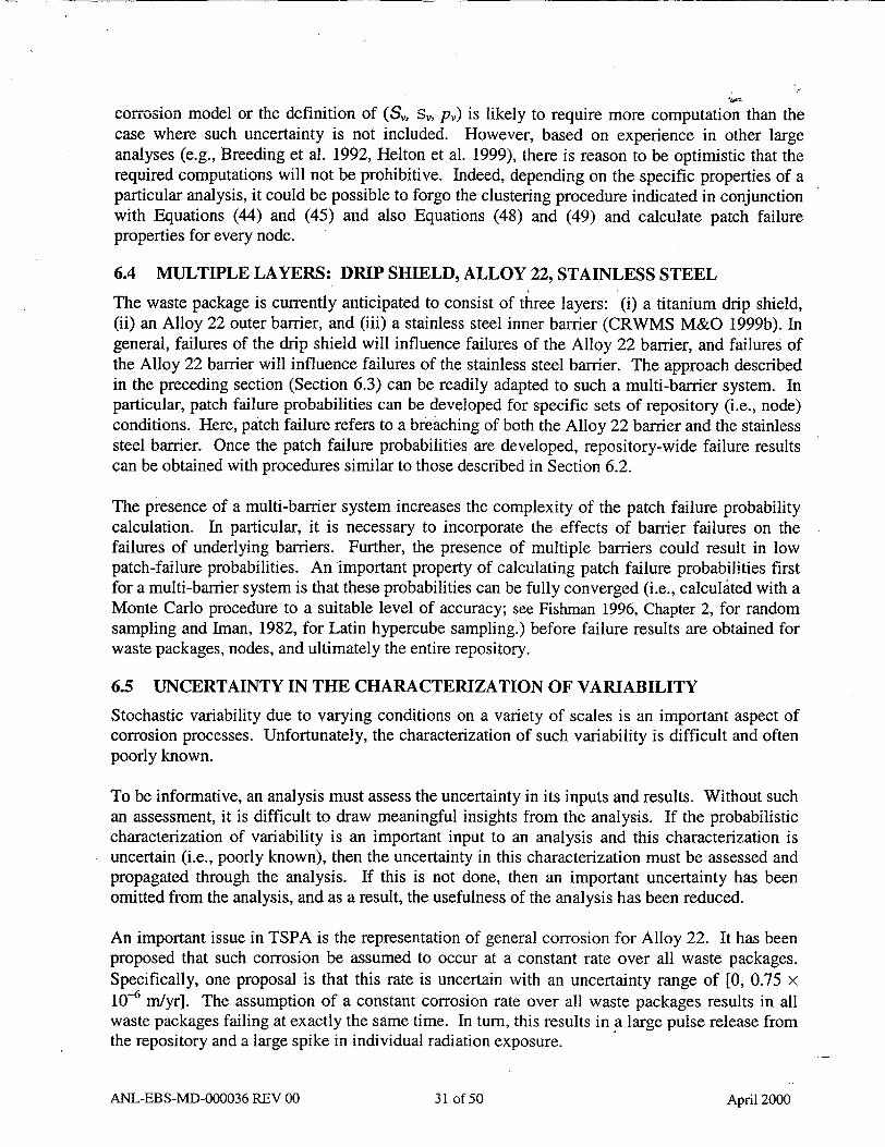
corrosion model or the definition of (S,, S,, Pv) is likely to require more computation than the case where such uncertainty is not included. However, based on experience in other large analyses (e.g., Breeding et al. 1992, Helton et al. 1999), there is reason to be optimistic that the required computations will not be prohibitive. Indeed, depending on the specific properties of a particular analysis, it could be possible to forgo the clustering procedure indicated in conjunction with Equations (44) and (45) and also Equations (48) and (49) and calculate patch failure properties for every node.

6.4 MULTIPLE LAYERS: DRIP SHIELD, ALLOY 22, STAINLESS STEEL

The waste package is currently anticipated to consist of three layers: (i) a titanium drip shield, (ii) an Alloy 22 outer barrier, and (iii) a stainless steel inner barrier (CRWMS M&O 1999b). In general, failures of the drip shield will influence failures of the Alloy 22 barrier, and failures of the Alloy 22 barrier will influence failures of the stainless steel barrier. The approach described in the preceding section (Section 6.3) can be readily adapted to such a multi-barrier system. In particular, patch failure probabilities can be developed for specific sets of repository (i.e., node) conditions. Here, patch failure refers to a breaching of both the Alloy 22 barrier and the stainless steel barrier. Once the patch failure probabilities are developed, repository-wide failure results can be obtained with procedures similar to those described in Section 6.2.

The presence of a multi-barrier system increases the complexity of the patch failure probability calculation. In particular, it is necessary to incorporate the effects of barrier failures on the failures of underlying barriers. Further, the presence of multiple barriers could result in low patch-failure probabilities. An important property of calculating patch failure probabilities first for a multi-barrier system is that these probabilities can be fully converged (i.e., calculated with a Monte Carlo procedure to a suitable level of accuracy; see Fishman 1996, Chapter 2, for random sampling and Iman, 1982, for Latin hypercube sampling.) before failure results are obtained for waste packages, nodes, and ultimately the entire repository.

6.5 UNCERTAINTY IN THE CHARACTERIZATION OF VARIABILITY

Stochastic variability due to varying conditions on a variety of scales is an important aspect of corrosion processes. Unfortunately, the characterization of such variability is difficult and often poorly known.

To be informative, an analysis must assess the uncertainty in its inputs and results. Without such an assessment, it is difficult to draw meaningful insights from the analysis. If the probabilistic characterization of variability is an important input to an analysis and this characterization is uncertain (i.e., poorly known), then the uncertainty in this characterization must be assessed and propagated through the analysis. If this is not done, then an important uncertainty has been omitted from the analysis, and as a result, the usefulness of the analysis has been reduced.

An important issue in TSPA is the representation of general corrosion for Alloy 22. It has been proposed that such corrosion be assumed to occur at a constant rate over all waste packages. Specifically, one proposal is that this rate is uncertain with an uncertainty range of [0, 0.75 x 10-6 m/yr]. The assumption of a constant corrosion rate over all waste packages results in all waste packages failing at exactly the same time. In turn, this results in a large pulse release from the repository and a large spike in individual radiation exposure.


A model that results in all waste packages failing at the same time is not reasonable and results from ignoring variability in the corrosion process that is generally accepted to exist (e.g., Farmer et al. 1991, Wu et al. 1991, Henshall 1992, Bullen 1996, Lyon et al. 1996). In particular, due to spatial variation arising from many sources (e.g., local variations in moisture, chemical conditions, surface properties, ... ), it is unlikely that small-scale environmental conditions will be identical throughout the repository, and thus that corrosion will take place at exactly the same rate throughout the repository.

If the preceding view is accepted, then there should be vwriability in the general corrosion rate across the repository. The fact that this variability is hard to quantify does not mean that it should be ignored. Rather, the implication is that there is a large amount of uncertainty in how this variability should be quantified. Omitting this variability and its associated uncertainty compromises the analysis in two ways. First, an inappropriate corrosion model is used (i.e., a spatially constant rather than spatially varying model). Second, an important uncertainty is omitted from the analysis (i.e., the uncertainty in how to characterize the variability in a corrosion process).

The characterization of the variability associated with general corrosion, or any other corrosion process, and the uncertainty in this characterization must come from individuals who are knowledgeable with respect to this process. Possibilities include triangular or log triangular distributions with uncertain minimums, modes and maximums, and normal or log normal distributions with uncertain means and standard deviations. It is unlikely that anyone will be fully satisfied with resultant characterizations of variability and uncertainty. However, an attempt at characterizing the variability and associated uncertainty in a corrosion process is more defensible than simply ignoring these important aspects of waste package and repository performance.

6.6 GAUSSIAN VARIANCE PARTITIONING

Gaussian variance partitioning starts with a distribution that involves both uncertainty and variability and then works backwards to obtain a distribution that characterizes variability and a distribution that characterizes uncertainty. In its simplest form, this procedure is based on the assumption that the variable of interest, y, has the form

y=m+v (Eq. 50)

and the distribution N( u,cr'+ a'), where m is a normal random variable with mean ji and 2 2 variance o-,, and v is a normal random variable with mean zero and variance or2. The

distribution associated with m, N( 'U, c-2), is assumed to characterize uncertainty, and the distribution associated with v, N(O, o•'), is assumed to characterize variability.

If jj, - and a' are known, then a sampling based analysis can be implemented that incorporates uncertainty by sampling m from N(/,o-,') and then, conditional on a sampled value for m, incorporates variability by sampling v from N(0,or2) to obtain multiple values of


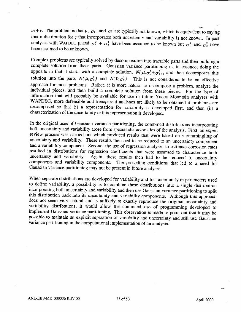
m + v. The problem is that p., a', and or' are typically not known, which is equivalent to saying that a distribution for y that incorporates both uncertainty and variability is not known. In past analyses with WAPDEG g. and or + o- have been assumed to be known but o- and o-' have been assumed to be unknown.

Complex problems are typically solved by decomposition into tractable parts and then building a complete solution from these parts. Gaussian variance partitioning is, in essence, doing the opposite in that it starts with a complete solution, N( 'aor +'Y ), and then decomposes this solution into the parts N( Iu,o') and N( O,o-). This -is not considered to be an effective approach for most problems. Rather, it is more natural to decompose a problem, analyze the individual pieces, and then build a complete solution from these pieces. For the type of information that will probably be available for use in future Yucca Mountain analyses with WAPDEG, more defensible and transparent analyses are likely to be obtained if problems are decomposed so that (i) a representation for variability is developed first, and then (ii) a characterization of the uncertainty in this representation is developed.

In the original uses of Gaussian variance partitioning, the combined distributions incorporating both uncertainty and variability arose from special characteristics of the analysis. First, an expert review process was carried out which produced results that were based on a commingling of uncertainty and variability. These results then had to be reduced to an uncertainty component and a variability component. Second, the use of regression analyses to estimate corrosion rates resulted in distributions for regression coefficients that were assumed to characterize both uncertainty and variability. Again, these results then had to be reduced to uncertainty components and variability components. The preceding conditions that led to a need for Gaussian variance partitioning may not be present in future analyses.

When separate distributions are developed for variability and for uncertainty in parameters used to define variability, a possibility is to combine these distributions into a single distribution incorporating both uncertainty and variability and then use Gaussian variance partitioning to split this distribution back into its uncertainty and variability components. Although this approach does not seem very natural and is unlikely to exactly reproduce the original uncertainty and variability distributions, it would allow the continued use of programming developed to implement Gaussian variance partitioning. This observation is made to point out that it may be possible to maintain an explicit separation of variability and uncertainty and still use Gaussian variance partitioning in the computational implementation of an analysis.


Failure Times 1 Sample, 100 Patches

0.10

Prob < t

0.00

09J2811999 17.09:19

0t, Time (y)

Note: Figure based on the Hypothetical Corrosion Model in Equation (1), the Characterization of Variability in Equations (7) and (8), and a Random Sample of Size nR = 100 (For illustration purposes only).

Figure 1. Estimate of Probability that Failure Time tf for a Single, Randomly Selected Patch Will Be Less Than or Equal to Time t.


10,000

34 of 50 April 2000

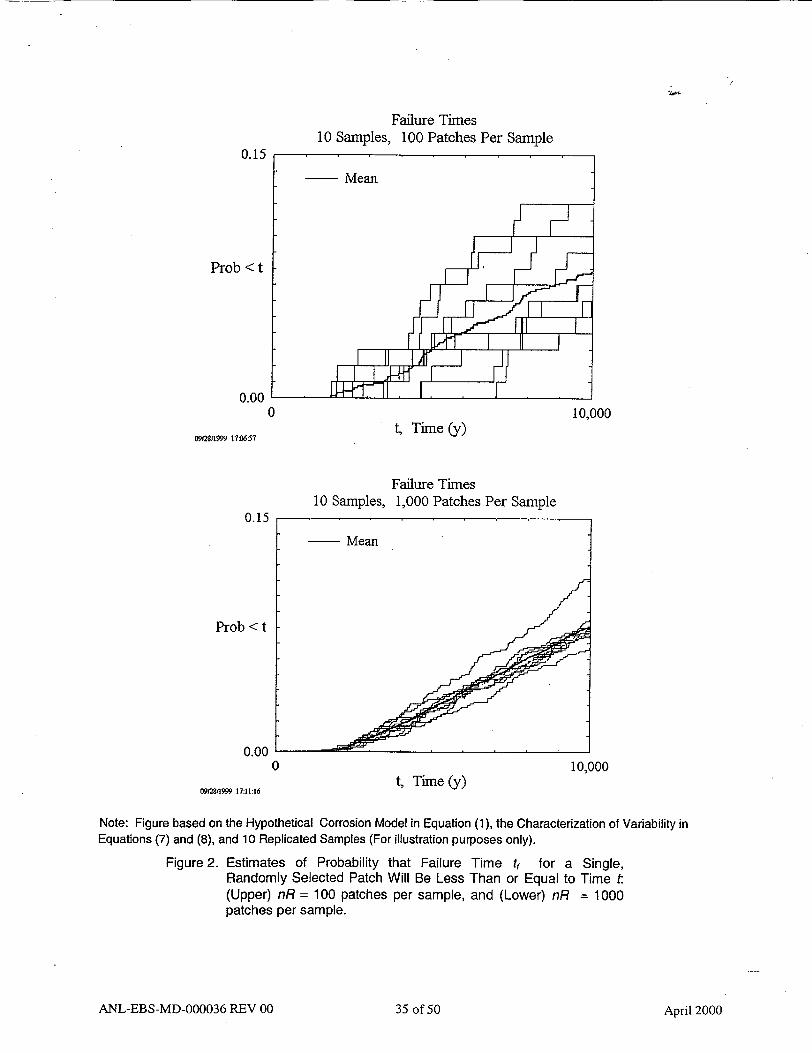
Failure Times 10 Samples, 100 Patches Per Sample

0.15

Prob < t

0.00

09=2S1999 17JO657

10 Samples,

10,000t, Time (y)

Failure Times 1,000 Patches Per Sample

t, Time (y)10,000

Note: Figure based on the Hypothetical Corrosion Model in Equation (1), the Characterization of Variability in Equations (7) and (8), and 10 Replicated Samples (For illustration purposes only).

Figure 2. Estimates of Probability that Failure Time tf for a Single, Randomly Selected Patch Will Be Less Than or Equal to Time t (Upper) nR = 100 patches per sample, and (Lower) nR = 1000 patches per sample.


0

0.15

Prob < t

0.00

09=281999 17:11:16

0

35 of 50 April 2000

Failure Times 10 Samples, 10,000 Patches Per Sample

t, Time (y)

Failure Times 10 Samples, 10,000 Patches Per Sample

t, Time (y)

Note: Figure based on (i) the Hypothetical Corrosion Model in Equation (1), (ii) the Characterization of Variability in Equations (7) and (8), (iii) the Characterization of Uncertainty in Equations (11)H16), (iv) a Random Sample xq,, j= 1,2,..., nS = 10, from S, (see Equation (23)), and (v) Use of a Random Sample xl,, i = 1,2,....nR = 104, from Sv in the Approximation of prob(tt< t I xuj)(see Equation (17)). (For illustration purposes only)

Figure 3. Estimates of Probability That Failure Time tf for a Single, Randomly Selected Patch Will Be Less Than or Equal to Time t (Upper) Individual Values for prob(tf•< t I xj), j = 1,2,..., nS, and (Lower) estimated mean and quantile curves for prob(tf< t I x,).


0.30

Prob < t

0.00

0I92=1999 21:14.21

0 10,000

0.30

Prob < t

0.00

09rMgtl999 22M.6.31

0 10,000

36 of 50 April 2000

Number of Patch Failures 10 Samples, 100 Patches Per Sample

15

Number of Failed Patches

0

09f2I1M999 17:14:56

150


0

0

09=21999 17:17n5

0t, Time (y)

Number of Patch Failures 10 Samples, 1,000 Patches Per Sample

10,000 t, Time (y)

Note: Figure based on the Hypothetical Corrosion Model in Equation (1), the Characterization of Variability in Equations (7) and (8), and 10 Replicated Samples (For illustration purposes only).

Figure 4. Example Number of Failed Patches on a Single Waste Package as a Function of Time: (Upper) nP = 100 patches, and (Lower) nP = 1000 patches.


10,000

37 of 50 April 2000

1.00

Prob < t

0.00 0

09M28A1999 16:54301

1.00

Prob < t

0.00

0

0912819 16L57.02

Early Failure Times 10 Samples, 100 Patches Per Sample

t, Time (y)8,000

Early Failure Times 10 Samples, 1000 Patches Per Sample

t, Time (y)8,000

Note: Figure based on Hypothetical Corrosion Model in Equation (1), the Characterization of Variability in Equations (7) and (8), and 10 Replicated Samples (For illustration purposes only).

Figure 5. Example of Cumulative Distribution Function (CDF) for Time of Initial Waste Package Failure: (Upper) nP = 100 patches and (Lower) nP = 1000 patches.


1.00

Prob < t

0.00 0

09F28/1999 17:24:05

1.00

Prob < t

0.00

0

09=281999 17:26:15

Early Failure Times 1,000 Samples, 100 Patches Per Sample

t, Time (y)10,000

Early Failure Times 1,000 Samples, 1,000 Patches Per Sample

t, Time (y)10,000

Note: Figure based on Hypothetical Corrosion Model in Equation (1), the Characterization of Variability in Equations (7) and (8), and 1000 Replicated Samples (For illustration purposes only).

Figure 6. Example of Cumulative Distribution Function (CDF) for Time of Initial Waste Package Failure: (Upper) nP = 100 patches and (Lower) nP = 1000 patches.



t, Time (y)


t, Time (y)

Note: Figure based on (i) the Hypothetical Corrosion Model in Equation (1), (ii) the Characterization of Variability in Equations (7) and (8), (iii) the Characterization of Uncertainty in Equations (11)-(16), (iv) a Random Sample xvj, j= 1,2,..., nS= 10, from Su (see Equation (23)), and (v) Use of a Random Sample x,, i= 1,2,..., nR= 104, from Svin the Approximation of p(tf< tI xuj)(see Equation (17)). (For illustration purposes only)

Figure 7. Example of Expected Number of Failed Patches on a Single Waste Package Divided into nP = 100 Patches as a Function of Time: (Upper) Individual Values for E(iI tnP= 100, xu,), j= 1,2,..., nS (see Equation (24)), and (Lower) Mean and Quantile Curves for E(iI tnP= 100, xe).


0

30


0

OMM/1999 21:I9•9

30


0

I 10fl999 09:M45

10,000

0 10,000

40 of 50 April 2000

1.00

Prob < t

0.00 0

09fMI999 1SOM3

1.00

Prob < t

0.00 0

09121999 18.49:43

Early Failure Times 100 Samples, 1,000 Early Failure Times Per CDF

(1,000 Samples, 100 Patches Per Sample)

t, Time (y)30,000

Early Failure Times 100 Samples, 1,000 Early Failure Times Per CDF

(1,000 Samples, 1,000 Patches Per Sample)

t, Time (y)30,000

Note: Figure based on (i) the Hypothetical Corrosion Model in Equation (1), (ii) the Characterization of Variability in Equations (7) and (8), (iii) the Characterization of Uncertainty in Equations (11)-(16), (iv) a Random Sample xu, j =

1,2,..., nS = 100, from S, (see Equation (23)), and (v) Use of 1000 Early Failure Times in the Generation of Each CDF

(For illustration purposes only).

Figure 8. Example of Cumulative Distribution Functions (CDFs) for Time of

Initial Waste Package Failure, tj: (Upper) nP = 100 patches, and (Lower) nP = 1000 patches.


7. CONCLUSIONS

Appropriate treatment of variability and uncertainty are important components of analyses for complex systems. Here, variability is being used to designate the inexactness that arises from consideration of a population in which the individual members have different properties, and uncertainty is being used to designate the inexactness that arises from a lack of knowledge about a quantity that is believed, or at least assumed in the context of a particular analysis, to have a fixed value (Section 6.1.1). The need to incorporate the effects of variability and uncertainty into analyses for complex systems is widely recognized (Section 6.1.2).

Analyses with models for corrosion processes involve both variability and uncertainty (Section 6.1.3). Variability in corrosion processes arises from spatial and possibly temporal variation in system properties on a scale beneath the level of resolution at which it is practicable to characterize such properties. Uncertainty arises from an inability to determine the exact mathematical forms of both corrosion models and probabilistic characterization for the variability associated with these models. In general, characterizations of both variability and uncertainty are analysis specific, with the specific details and context of an analysis determining how variability should be represented and the level of uncertainty present in the analysis. Often, the appropriate way to characterize variability is one of the major uncertainties in an analysis.

The basic unit used by WAPDEG in the representation of the effects of variability in corrosion processes is a patch, which is a small area of homogeneous conditions on a waste package. By appropriately calculating the effects of variability over patches, computational procedures can be developed that allow the efficient computation of failure results for waste packages, groups of waste packages, and ultimately, all waste packages in the repository (Sects. 6.2, 6.3, 6.4). Specifically, Monte Carlo procedures can be used to assure that failure results for patches are determined to a level of resolution that fully captures the effects of variability; then, direct calculations based on established procedures for manipulating probabilities (e.g., the binomial theorem) can be used to determine failure results for waste packages. Further, these procedures can be developed so that a separation between variability and uncertainty is maintained.

In meetings on the design of TSPA calculations, concern has been expressed about both (i) the computational cost of the corrosion calculations to be carried out by WAPDEG and (ii) a possible lack of resolution in the incorporation of the effects of variability in corrosion processes and other failure mechanisms across all the waste packages in the repository. Unfortunately, increasing the resolution of the calculations also increases the computational cost of the analysis. The computational procedures introduced Sects. 6.3-6.4 offer a possible solution to this problem that could both increase the resolution at which variability is incorporated into the analysis and reduce the overall computational cost. In particular, it could be possible to increase resolution and decrease computational cost by using WAPDEG to determine patch failure probabilities and other TSPA codes to determine repository-wide waste package failure from these probabilities.

Unrealistic models should not be used as a substitute for characterizing the uncertainty in a representation for variability (Section 6.5). Variability is often hard to describe. An informative analysis should provide an assessment of the uncertainty in its inputs and the effects that this uncertainty has on important analysis outcomes. If variability is an important but uncertain input


to an analysis, then this uncertainty should be incorporated into the analysis in a way that allows its effects and importance to be assessed.

Past analyses with WAPDEG have started with distributions that incorporated the effects of both variability and uncertainty and then used Gaussian variance partitioning to separate the effects of uncertainty from the effects of variability (Section 6.6). Although the use of this partitioning procedure is appropriate in some analysis situations, more defensible and transparent analyses are more likely to be obtained in most situations if problems are decomposed so that (i) a representation for variability is developed, and then (ii) a characterization of the uncertainty in this representation is developed.


8. REFERENCES

8.1 DOCUMENTS CITED

Allen, B.C.; Covington, T.R.; and Clewell, H.J. 1996. "Investigation of the Impact of Pharmacokinetic Variability and Uncertainty on Risks Predicted with a Phanmacokinetic Model for Chloroform." Toxicology, 111, 289-303. New York, New York: Elsevier. TIC: 245771.

Anderson, E.; Deisler, P.F., Jr.; McCallum, D.; St. Hilaire,' C.; Spitzer, H.L.; Strauss, H.; Wilson, J.D.; and Zimmerman, R. 1993. "Key Issues in Carcinogen Risk Assessment Guidelines, Society for Risk Analysis." Risk Analysis, 13, (4), 379-382. New York, New York: Plenum Press. TIC: 245815.

Apostolakis, G. 1990. "The Concept of Probability in Safety Assessments of Technological Systems." Science, 250, 1359-1364. Washington, D.C.: American Association for the Advancement of Science. TIC: 212560.

Apostolakis, G.E. 1989. "Uncertainty in Probabilistic Safety Assessment." Nuclear Engineering and Design, 115, (1), 173-179. Amsterdam, The Netherlands: Elsevier Science Publishers. TIC: 245806.

Bernstein, P.L. 1996. Against the Gods: The Remarkable Story of Risk. New York, New York: John Wiley and Sons. TIC: 245429.

Bogen, K.T. and Spear, R.C. 1987. "Integrating Uncertainty and Interindividual Variability in Environmental Risk Assessment." Risk Analysis, 7, (4), 427-436. New York, New York: Plenum Press. TIC: 245810.

Brattin, W.J.; Barry, T.M.; and Chiu, N. 1996. "Monte Carlo Modeling with Uncertain Probability Density Functions." Human and Ecological Risk Assessment, 2, (4), 820-840. Amherst, Massachusetts: Amherst Scientific Publishers. TIC: 246157.

Breeding, R.J.; Helton, J.C.; Gorham, E.D.; and Harper, F.T. 1992. "Summary Description of the Methods Used in the Probabilistic Risk Assessments for NUREG-1150." Nuclear Engineering and Design, 135, 1-27. New York, New York: Elsevier Science Publishers. TIC: 246312.

Bullen, D.B. 1996. "A Model for Container Performance in an Unsaturated Repository." Nuclear Technology, 113, (1), 29-45. La Grange Park, Illinois: American Nuclear Society. TIC: 245804.

CRWMS M&O (Civilian Radioactive Waste Management System Management and Operating Contractor) 1998. "Waste Package Degradation Modeling and Abstraction." Chapter 5 of Total System Performance Assessment-Viability Assessment (TSPA-VA) Analyses Technical Basis Document. BOOOOOOOO-01717-4301-00005 REV 01. Las Vegas, Nevada: CRWMS M&O. ACC: MOL. 19981008.0005.


CRWMS M&O 1999a. Incorporation of Uncertainty and Variability of Drip Shield and Waste Package Degradation in WAPDEG Analysis. TDP-EBS-MD-000020 REV 00. Las Vegas, Nevada: CRWMS M&O. ACC: MOL.19990813.0389.

CRWMS M&O 1999b. Monitored Geologic Repository Project Description Document. BOOOOOOOO-01717-1705-00003 REV 00 DCN 01. Las Vegas, Nevada: CRWMS M&O. ACC: MOL.19991117.0160.

Cullen, A.C. and Frey, H.C. 1999. Probabilistic Techniques in Exposure Assessment, A Handbook for Dealing with Variability and Uncertainty in Models and Inputs. New York, New York: Plenum Press. TIC: 242815.

DOE (U.S. Department of Energy) 1998. Viability Assessment of a Repository at Yucca Mountain. DOE/RW-0508. Washington, D.C.: U.S. Department of Energy, Office of Civilian Radioactive Waste Management. ACC: MOL.19981007.0027; MOL.19981007.0028; MOL. 19981007.0029; MOL. 19981007.0030; MOL. 19981007.0031; MOL. 19981007.0032.

DOE 2000. Quality Assurance Requirements and Description. DOE/RW-0333P, Rev. 9. Washington, D.C.: U.S. Department of Energy, Office of Civilian Radioactive Waste Management. ACC: MOL. 19991028.0012.

EPA (U.S. Environmental Protection Agency) 1997. Guiding Principles for Monte Carlo Analysis. EPA/630/R-97/001. Washington, D.C.: Environmental Protection Agency. TIC: 244010.

Farmer, J.C.; Gdowski, G.E.; McCright, R.D.; and Ahluwahlia, H.S. 1991. "Corrosion Models for Performance Assessment of High-Level Radioactive-Waste Containers." Nuclear Engineering and Design, 129, (1), 57-88. Amsterdam, The Netherlands: Elsevier Science Publishers. TIC: 245851.

Feller, W. 1971. "Wiley Series in Probability and Mathematical Statistics." An Introduction to Probability Theory and Its Applications. Volume II, 2nd Edition, 654 p. New York, New York: John Wiley & Sons. TIC: 235188.

Finkel, A.M. 1990. Confronting Uncertainty in Risk Management, A Guide for Decision-Makers. Washington, D.C.: Center for Risk Management, Resources for the Future. TIC: 247070.

Fishman, G.S. 1996. Monte Carlo, Concepts, Algorithms, and Applications. Springer Series in Operations Research. New York, New York: Springer-Verlag. TIC: 247103.

Fogarty, J.J.; Rosenberg, A.A.; and Sissenwine, M.P. 1992. "Fisheries Risk Assessment: Sources of Uncertainty: A Case Study of Georges Bank Haddock." Environmental Science and Technology, 26, (3), 440-447. Washington, D.C.: American Chemical Society. TIC: 245874.

Frey, H.C. and Rhodes, D.S. 1996. "Characterizing, Simulating, and Analyzing Variability and Uncertainty: An Illustration of Methods Using an Air Toxics Emissions Example." Human and


Ecological Risk Assessment, 2, (4), 762-797. Amherst, Massachusetts: Amherst Scientific Publishers. TIC: 246162.

Hacking, 1. 1975. The Emergence of Probability: A Philosophical Study of Early Ideas about Probability, Induction and Statistical Inference. New York, New York: Cambridge University Press. TIC: 245428.

Hansen, P. and Jaumard, B. 1997. "Cluster Analysis and Mathematical Programming." Mathematical Programming, 79, 191-215. Amsterdam, The Netherlands: Elsevier Science B.V. TIC: 247082.

Hattis, D. and Silver, K. 1994. "Human Interindividual Variability-A Major Source of Uncertainty in Assessing Risks for Noncancer Health Effects." Risk Analysis, 14, (4), 421-43 1. New York, New York: Plenum Press. TIC: 245863.

Helton, J.C. 1993. "Risk, Uncertainty in Risk, and the EPA Release Limits for Radioactive Waste Disposal." Nuclear Technology, 101, (1), 18-39. La Grange Park, Illinois: American Nuclear Society. TIC: 245799.

Helton, J.C. 1994. "Treatment of Uncertainty in Performance Assessments for Complex Systems." Risk Analysis, 14, (4), 483-511. New York, New York: Plenum Press. TIC: 245848.

Helton, J.C. 1996. "Probability, Conditional Probability and Complementary Cumulative Distribution Functions in Performance Assessment for Radioactive Waste Disposal." Reliabilty Engineering and System Safety, 54, 145-163. Oxford, United Kingdom: Elsevier. TIC: 246183.

Helton, J.C. 1997. "Uncertainty and Sensitivity Analysis in the Presence of Stochastic and Subjective Uncertainty." Journal of Statistical Computation and Simulation, 57, (1-4), 3-76. New York, New York: Gordon and Breach Science Publishers. TIC: 245958.

Helton, J.C. and Burmaster, D.E. 1996. "Guest Editorial: Treatment of Aleatory and Epistemic Uncertainty in Performance Assessments for Complex Systems." Reliability Engineering and System Safety, 54, 91-94. New York, New York: Elsevier Science Limited. TIC: 245900.

Helton, J.C.; Anderson, D.R.; Jow, H.-N.; Marietta, M.G.; and Basabilvazo, G. 1999. "Performance Assessment in Support of the 1996 Compliance Certification Application for the Waste Isolation Pilot Plant." Risk Analysis, 19, (5), 959-986. New York, New York: Plenum Press. TIC: 247081.

Henshall, G.A. 1992. "Modeling Pitting Corrosion Damage of High-Level Radioactive-Waste Containers Using a Stochastic Approach." Journal of Nuclear Materials, 195, (1-2), 109-125. Amsterdam, The Netherlands: Elsevier. TIC: 237758.

Hoffman, F.O. and Hammonds, J.S. 1994. "Propagation of Uncertainty in Risk Assessments: The Need to Distinguish Between Uncertainty Due to Lack of Knowledge and Uncertainty Due to Variability." Risk Analysis, 14, (5), 707-712. New York, New York: Plenum. TIC: 246313.


IAEA (International Atomic Energy Agency) 1989. Evaluating the Reliability of Predictions Made Using Environmental Transfer Models. Safety Series No. 100. Vienna, Austria: International Atomic Energy Agency. TIC: 246629.

Iman, R.L. 1982. "Statistical Methods for Including Uncertainties Associated with the Geologic Isolation of Radioactive Waste Which Allow for a Comparison with Licensing Criteria." Proceedings of the Symposium on Uncertainties Associated with the Regulation of the Geologic Disposal of High-Level Radioactive Waste, Gatlinburg, Tennessee, March 9-13, 1981. Kocher, D.C., ed. NUREG/CP-0022, 145-157. Washington, D.C.: U.S. Nuclear Regulatory Commission. TIC: 213069.

Iman, R.L.; Helton, J.C.; and Johnson, J.D. 1990. "A Methodology for Grouping Source Terms for Consequence Calculations in Probabilistic Risk Assessments." Risk Analysis, 10, (4), 507520. New York, New York: Plenum Press. TIC: 247090.

Kaplan, S. 1993. "Formalisms for Handling Phenomenological Uncertainties: The Concepts of Probability, Frequency, Variability, and Probability of Frequency." Nuclear Technology, 102, (1), 137-142. La Grange Park, Illinois: American Nuclear Society. TIC: 245866.

Kaplan, S. and Garrick, B.J. 1981. "On the Quantitative Definition of Risk." Risk Analysis, 1, (1), 11-27. New York, New York: Plenum Press. TIC: 241205.

Lewis, H.W.; Budnitz, R.J.; Kouts, H.J.C.; Loewenstein, W.B.; Rowe, W.D.; von Hippel, F.; and Zachariasen, F. 1978. Risk Assessment Review Group Report to the U.S. Nuclear Regulatory Commission. NUREG/CR-0400. Washington, D.C.: U.S. Regulatory Commission. TIC: 206094.

Lyon, B.F.; Holmes, J.A.; Kosiewicz, S.T.; Wilbert, K.A.; and Travis, C.C. 1996. "Estimation of Corrosion on Carbon Steel TRU Waste Drums Using the Poisson Distribution." Journal of Hazardous Materials, 51, 165-179. New York, New York: Elsevier Science Publishing. TIC: 245801.

MacIntosh, D.L.; Suter, G.W., II; and Hoffman, F.O. 1994. "Uses of Probabilistic Exposure Models in Ecological Risk Assessments of Contaminated Sites." Risk Analysis, 14, (4), 405-419. New York, New York: Plenum Press. TIC: 245847.

McKone, T.E. 1994. "Uncertainty and Variability in Human Exposures to Soil Contaminants Through Home-Grown Food: A Monte Carlo Assessment." Risk Analysis, 14, (4), 449-463. New York, New York: Plenum Press. TIC: 245846.

McKone, T.E. and Bogen, K.T. 1991. "Predicting the Uncertainties in Risk Assessment: A California Groundwater Case Study." Environmental Science and Technology, 25, (10), 16741681. Washington, D.C.: American Chemical Society. TIC: 245869.

National Council on Radiation Protection and Measurements 1996. A Guide for Uncertainty Analysis in Dose and Risk Assessments Related to Environmental Contamination. NCRP


Commentary No. 14. Bethesda, Maryland: National Council on Radiation Protection and Measurements. TIC: 245979.

National Research Council 1983. Risk Assessment in the Federal Government: Managing the Process.. Washington, D.C.: National Academy Press. TIC: 246298.

National Research Council 1994. Science and Judgment in Risk Assessment. Washington, D.C.: National Academy Press. TIC: 215158.

National Research Council. 1993. "Issues in Risk Assessrhent ." Committee on Risk Assessment Methodology, Board on Environmental Studies and Toxicology, Commission on Life Sciences and the National Research Council. First in a Series, 350 p. Washington, D.C.: National Academy Press. TIC: 231814.

NRC (Nuclear Regulatory Commission) 1975. Reactor Safety Study: An Assessment of Accident Risks in U.S. Commercial Nuclear Power Plants. WASH-1400. Washington, D.C.: U.S. Nuclear Regulatory Commission. TIC: 236923.

NRC 1990. Severe Accident Risks: An Assessment for Five U.S. Nuclear Power Plants. NUREG1150. Washington, D.C.: U.S. Regulatory Commission. TIC: 214826.

Parry, G.W. 1988. "On the Meaning of Probability in Probabilistic Safety Assessment." Reliability Engineering and System Safety, 23, (4), 309-314. New York, New York: Elsevier Applied Science. TIC: 245959.

Pate-Cornell, M.E. 1996. "Uncertainties in Risk Analysis: Six Levels of Treatment." Reliability Engineering and System Safety, 54, (2-3), 95-111. New York, New York: Elsevier Science Limited. TIC: 245961.

Payne, A.C., Jr. 1992. Analysis of the LaSalle Unit 2 Nuclear Power Plant: Risk Methods Integration and Evaluation Program (RMIEP). NUREG/CR-4832. Albuquerque, New Mexico: Sandia National Laboratories. TIC: 246147.

PLG (Pickard, Lowe and Garrick) 1983a. Seabrook Station Probabilistic Safety Assessment, Main Report. PLG-0300, Rev. 2. Sections 1-3. Irvine, California: Pickard, Lowe and Garrick. TIC: 247420.

PLG (Pickard, Lowe, and Garrick) 1983b. Seabrook Station Probabilistic Safety Assessment. PLG-0300, Rev. 2. Sections 4-13. Irvine, California: Pickard, Lowe and Garrick. TIC: 247143.

Price, P.S.; Su, S.H.; Harrington, J.R.; and Keenan, R.E. 1996. "Uncertainty and Variation in Indirect Exposure Assessments: An Analysis of Exposure to Tetrachlorodibenzo-p-Dioxin from a Beef Consumption Pathway." Risk Analysis, 16, (1), 263-277. New York, New York: Plenum Press. TIC: 245868.


Rai, S.N.; Krewski, D.; and Bartlett, S. 1996. "A General Framework for the Analysis of uncertainty and Variability in Risk Assessment." Human and Ecological Risk Assessment, 2, (4), 972-989. Amherst, Massachusetts: Amherst Scientific Publishers. TIC: 246158.

Ross, S.M. 1993. Introduction to Probability Models. 5th Edition. Section 2.2.2. San Diego, California: Academic Press. TIC: 245879.

Silbergeld, E.K. 1987. "Five Types of Ambiguity: Scientific Uncertainty in Risk Assessment." Hazardous Waste and Hazardous Materials, 4, (2), 139-150. New York, New York: Mary Ann Liebert Publishers. TIC: 245962.

Thompson, K.M. and Graham, J.D. 1996. "Going Beyond the Single Number: Using Probabilistic Risk Assessment to Improve Risk Management." Human and Ecological Risk Assessment, 2, (4), 1008-1034. Amherst, Massachusetts: Amherst Scientific Publishers. TIC: 246163.

U.S. Environmental Protection Agency 1993. An SAB Report: Multi-Media Risk Assessment for Radon: Review of Uncertainty Analysis of Risks Associated with Exposure to Radon. EPA-SABRAC-93-014. Washington, D.C.: U.S. Environmental Protection Agency, Science Advisory Board. TIC: 246314.

Vesely, W. E. and Rasmuson, D. M. 1984. "Uncertainties in Nuclear Probabilistic Risk Analyses." Risk Analysis, 4, (4), 313-322. New York, New York: Plenum Press. TIC: 245875.

Whipple, C.G. 1986. "Dealing With Uncertainty About Risk in Risk Management." Part 1 Hazards: Technology and Fairness. 44-59. Washington, D.C.: National Academy Press. TIC: 245813.

Winkler, R.L. 1996. "Uncertainty in Probabilistic Risk Assessment." Reliability Engineering and System Safety, 54, (2-3), 127-132. New York, New York: Elsevier Science Limited. TIC: 245960.

Wu, Y.T.; Journel, A.G.; Abramson, L.R.; and Nair, P.K. 1991. Uncertainty Evaluation Methods for Waste Package Performance Assessment. NUREG/CR-5639. Washington, D.C.: U.S. Nuclear Regulatory Commission. TIC: 234497.

8.2 CODES, STANDARDS, REGULATIONS, AND PROCEDURES

50 FR 38066 (1985). 40 CFR Part 191: Environmental Standards for the Management and Disposal of Spent Nuclear Fuel, High-Level and Transuranic Radioactive Wastes; Final Rule. Readily Available

51 FR 30028. Safety Goals for the Operations of Nuclear Power Plants; Policy Statement; Republication. Readily Available


-- C

58 FR 66398 (1993). 40 CFR Part 191: Environmental Radiation Protection Standards for the Management and Disposal of Spent Nuclear Fuel, High-Level and Transuranic Radioactive Wastes; Final Rule. Readily Available

61 FR 5224. Criteria for the Certification and Re-Certification of the Waste Isolation Pilot Plant's Compliance with the 40 CFR Part 191 Disposal Regulations; Final Rule. Readily Available

AP-2.13Q, Rev. 0, ICN 0. Technical Product Development Planning. Washington, D.C.: U.S. Department of Energy, Office of Civilian Radioactive Waste Management. ACC: 19990701.0617.

AP-3.1Q Rev. 0, ICN 1. Conduct of Performance Assessment. Washington, D.C.: U.S. Department of Energy, Office of Civilian Radioactive Waste Management. ACC: MOL.19990304.0214.

AP-3.10Q, Rev. 2, ICN 0. Analyses and Models. Washington, D.C.: U.S. Department of Energy, Office of Civilian Radioactive Waste Management. ACC: MOL. 19991019.0467.

NLP-2-0. Rev. 5. Determination of Importance Evaluations. Washington, D.C.: U.S. Department of Energy, Office of Civilian Radioactive Waste Management. ACC: MOL. 19981116.0120.

QAP-2-0, Rev. 5, ICN 1. Conduct of Activities. Washington, D.C.: U.S. Department of Energy, Office of Civilian Radioactive Waste Management. ACC: MOL.19991109.0221.


Revision 00 of ANL-EBS-MD-000036, 'Incorporation of ... · MANAGEMENT ANALYSIS/MODEL REVISION...

Documents

Transcript of Revision 00 of ANL-EBS-MD-000036, 'Incorporation of ... · MANAGEMENT ANALYSIS/MODEL REVISION...