Y. B. Li and W. Zhou, Numerical Simulation of Filling Process in Die Casting, Materials Technology, Vol. 18, No. 1, 2003, pp. 36-41.

Numerical Simulation of Filling Process in Die Casting

Li Yongbao * and Wei Zhou **

Affiliation of authors: * School of Mechanical & Production Engineering Nanyang Technological University 50 Nanyang Avenue Singapore 639798 ** Division of Engineering & Applied Sciences Harvard University 9 Oxford Street Cambridge, MA 02138-2901, USA

Author for correspondence: Wei Zhou E-mail: wzhou@cantab.net

Acknowledgments The authors would like to thank Dr. Markus Schmid in ARGE Metallguss, Germany for providing the

experimental results on water analogy. One of the authors (WZ) would like to thank Dr. Hu Banghong

and Prof. David Taplin for helpful discussion and Nanyang Technological University for financial

support through AcRF 79/98.

1

Numerical Simulation of Filling Process in Die Casting

Li Yongbao and Wei Zhou

Abstract Mould filling in high pressure die casting is a complex process where performance is governed by a

number of design variables. The small heat capacity of magnesium alloys, combining with low

density, results in the magnesium molten mass chilling very rapidly. This makes the modeling of

filling process in magnesium die casting more important in assuring the quality of casting. In order to

realize this objective, a 3-D software program using FDM is developed to simulate the filling process.

This program includes a mesh generation module, a solver, a post-processor and a Graphic User

Interface (GUI). SMAC method was used to solve the full Navier-Stokes equations and track the free

surface, and the κ-ε model to account for the turbulence phenomenon during filling process. The

simulation results were shown to be in good agreement with the experimental results.

Keywords: die casting, filling process, numerical simulation, magnesium Nomenclature c Specific heat, J/g⋅K Cµ, C1, C2 Empirical constants in the k-ε model gx, gy , gz Gravitational constant in vector notation corresponding to x, y, z directions, cm/s2 k Thermal conductivity, W/cm⋅K K Turbulence kinetic energy, cm2/s2 p Pressure, g/cm⋅s2 S An energy source t Time, s T Temperature, K u, v, w Velocity components in x, y, z directions, m/s α Over-relaxation parameter, 0.5 to 0.7 γ Coefficient of kinematic viscosity δ Prescribed tolerance, 2×10-4 ε Dissipation rate of turbulence kinetic energy, cm2/s3 µ Molecular viscosity, cm2/s µe Effective viscosity, cm2/s µt Apparent viscosity, cm2/s ρ Density of melt, g/m3

σk, σε Schmidt numbers for K and ε ψ Potential function

2

1 Introduction Magnesium alloys offer attractive properties, particularly a high strength-to-weight ratio, which

makes them particularly ideal for components requiring low weight. High pressure die casting is the

most attractive manufacturing route for these components. With better fluidity than aluminum,

magnesium is highly suitable for production of components with long and thin sections. However, due

to the significantly lower thermal capacity of magnesium, molten magnesium will solidify very

rapidly during mould filling process. Today's die casting is still largely empirical in design and

process control. The result is greater difficulties in magnesium alloy die casting than in aluminum.

Porosity in die castings is a major defect limiting further applications [1-2]. Numerical simulation was

introduced in order to improve the running system design of die casting process and eliminate

porosity and cold shut in magnesium alloy castings [3-5]. Because of the high inlet speed and

turbulent flow, it is more challenging to simulate the mould-filling process during die casting than in

sand casting process.

The molten metal in die casting can be regarded as Newtonian fluid; therefore, to model the fluid flow

in die castings, the complete Navier-Stokes equations need to be used to calculate transient velocity

and pressure changes and the κ-ε model must be used to account for turbulence. The two most

important numerical methods employed in casting simulation are Finite Difference Method (FDM)

and Finite Element Method (FEM). FDM is relatively easy to program and it produces results with

reasonable accuracy [6-8], although FEM has been shown to have advantages over FDM for modeling

thin-walled castings [9-10]. Recently, Smoothed Particle Hydrodynamics (SPH), a meshless method

for solving physical problems governed by partial differential equations, has been used to model high

pressure die casting [11]. With the development of numerical methods, Boundary Element Method

(BEM) has also been used in the modeling of the filling process [12].

The main task in modeling the filling process of die casting is the solution to the N-S equations and

determination of free surface. In earlier studies, two computational fluid dynamic s techniques, namely

MAC (Marker and Cell) [13-14] and SOLA-VOF (SOLution Algorithm and Volume of Fluid) [15-

3

16], have been found to be suitable to treat fluid flow problems of this kind. Based on MAC the

SMAC (Simplified MAC) method was developed, in which the pressure does not need be calculated

[17]. The two main methods of tracking free surface during time-dependent flow are VOF and MAC

[6-16].

In the present study, a three dimensional program was developed to analyze the filling process of die

casting. The program includes a solver, pre- and post-processors. In order to achieve the main task of

this program in a limited period, STereo Lithography (STL) file was used to input geometric models

from commercial CAD software packages such as Pro/Engineering. STL files can keep all the

identities of the model (compared with IGES files) even though triangular facets are used in STL to

approximate curved surfaces. The detailed algorithm of the mesh generation can be found in reference

[18]. Simulation results from the program were found to be in good agreement with experiment.

2 Mathematical Model The mathematical model of mould filling process is obtained from momentum, mass and energy

conservation. These equations are as follows:

Continuity equation:

0zw

yv

xu =

∂∂+

∂∂+

∂∂ (1)

Momentum equations:

∂∂

+∂∂

+∂∂

γ++∂∂

ρ−=

∂∂

+∂∂

+∂∂

+∂∂

2

2

2

2

2

2

xz

u

y

u

x

ug

x

p1

z

uw

y

uv

x

uu

t

u (2)

∂∂

+∂∂

+∂∂

γ++∂∂

ρ−=

∂∂

+∂∂

+∂∂

+∂∂

2

2

2

2

2

2

yz

v

y

v

x

vg

y

p1

z

vw

y

vv

x

vu

t

v (3)

∂∂

+∂∂

+∂∂

γ++∂∂

ρ−=

∂∂

+∂∂

+∂∂

+∂∂

2

2

2

2

2

2

zz

w

y

w

x

wg

zp1

zw

wyw

vxw

utw (4)

Energy equation:

Sz

T

y

T

x

T

c

k

z

Tw

y

Tv

x

Tu

t

T2

2

2

2

2

2

+

∂∂

+∂∂

+∂∂

ρ=

∂∂

+∂∂

+∂∂

+∂∂

(5)

4

where, ρ is density, γ is the coefficient of kinematic viscosity, gx, gy and gz are vector components of

gravity, u, v and w are velocity components in x, y and z directions respectively, p is pressure, k is

thermal conductivity, c is specific heat, T is temperature and S is a heat source term.

It should be realized that for most problems in casting, especially in high pressure die casting, the

fluid flow is turbulent during the filling stage. Since turbulence is a very effective means for mass,

momentum and energy transport, it has a significant effect on the viscosity. Among the turbulence

models it is the turbulence transport equations which are more difficult and time consuming to

implement than other models. It is, however, the simplest turbulence model, for which only initial

and/or boundary conditions need to be supplied. In particular the κ-ε model (two-equation model) is

well established and the most widely validated turbulence model because of its excellent performance

for many applications. The κ-ε model [19] was therefore adopted in this study.

The dependent variables in N-S equations were replaced with time averages plus fluctuations. After

time averaging, the same form of continuity and momentum equations (see equations 1-4) can be

obtained for incompressible flow, except that the molecular viscosity is replaced by effective viscosity

µe (i.e. the sum of molecular viscosity µ and apparent viscosity µt). The key to solving the momentum

equation of turbulent flow is to determine the apparent viscosity. The two-equation model is

introduced to define the value of µt.

The standard κ-ε model uses the following transport equations for turbulent kinetic energy κ and the

rate of dissipation per unit mass ε:

ρε−+∂∂

⋅σµ

+µ∂∂

=ρ∂∂

+ρ∂∂

kjk

t

jj

j

P)x

K(

x)Ku(

x)K(

t (6)

)CPC(K

)x

(x

)u(x

)(t 2k1

j

t

jj

j

ρε−ε

+∂∂ε

⋅σµ

+µ∂∂

=ερ∂∂

+ρε∂∂

ε

(7)

where

)x

u

x

u(

x

uP

i

j

j

i

i

itk ∂

∂+

∂∂

∂∂

µ=

(8)

5

Then µt can be expressed as follows:

ερ=µ µ KC 2t

(9)

The equations contain five constants Cµ, σk, σε, C1 and C2. The standard κ-ε model employs values for

the constants that are arrived at by comprehensive data fitting for a wide range of turbulent flows. The

values are listed in Table 1.

Table 1 Values of the constants in standard κ-ε model [19]

Cµ C1 C2 σε σκ

0.09 1.44 1.92 1.3 1.0

3 Numerical Solution A simplified MAC (SMAC) method was adopted based on MAC [17]. In MAC the velocity and

pressure fields are solved explicitly and an iterative procedure is normally needed for the solution of

the Poisson equation for the pressure field. However, pressure needs not be calculated in SMAC.

According to the SMAC method, an arbitrary pressure field is first assigned to solve for the new time

step velocities field (tentative velocity field) and then this tentative velocity field is altered by the

addition of the gradient of an appropriate potential function ψ. If the velocity potential function at the

new time step can be obtained, the velocity field can be corrected and has zero divergence.

In order to convert the tentative velocity field into the final velocity field so that divergence

0D k,j,i = for every cell, the change in each velocity was given by the gradient of the potential

function. This, together with the requirement 0D 1nk,j,i ≡+ and appropriate boundary conditions allowed

the value of ψi , j , k for every cell to be determined uniquely. In order to accumulate the computation

speed, an over-relaxation method was adopted. The equation for the ψ at each new time step is given

by:

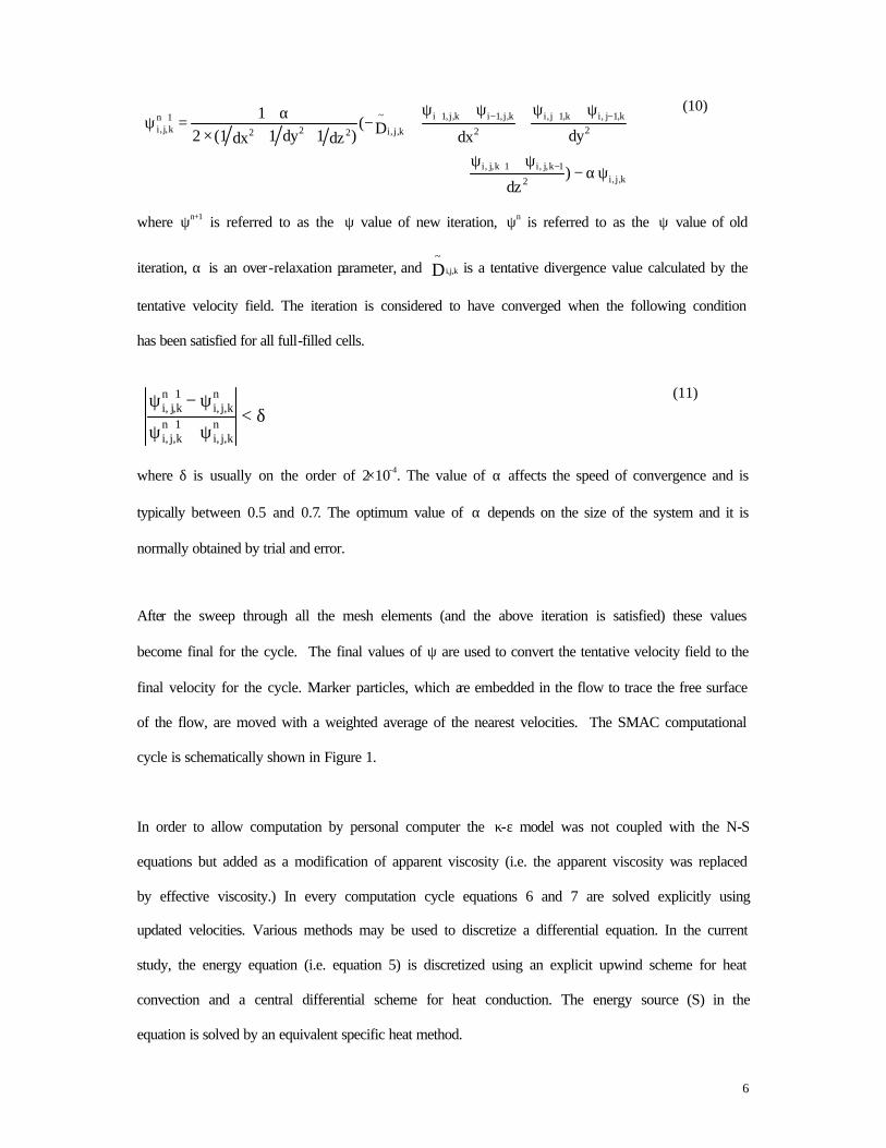
6

ψα−ψ+ψ

+

ψ+ψ+

ψ+ψ+−

++×α+=ψ

−+

−+−++

k,j,i2

1k,j,i1k,j,i

2

k,1j,ik,1j,i

2

k,j,1ik,j,1i~

k,j,i222

1nk,j,i

)dz

dydxD()dz1dy1dx1(2

1

(10)

where ψn+1 is referred to as the ψ value of new iteration, ψn is referred to as the ψ value of old

iteration, α is an over-relaxation parameter, and D~

i,j,k is a tentative divergence value calculated by the

tentative velocity field. The iteration is considered to have converged when the following condition

has been satisfied for all full-filled cells.

δ<ψ+ψ

ψ−ψ+

+

nk,j,i

1nk,j,i

nk,j,i

1nk,j,i

(11)

where δ is usually on the order of 2×10-4. The value of α affects the speed of convergence and is

typically between 0.5 and 0.7. The optimum value of α depends on the size of the system and it is

normally obtained by trial and error.

After the sweep through all the mesh elements (and the above iteration is satisfied) these values

become final for the cycle. The final values of ψ are used to convert the tentative velocity field to the

final velocity for the cycle. Marker particles, which are embedded in the flow to trace the free surface

of the flow, are moved with a weighted average of the nearest velocities. The SMAC computational

cycle is schematically shown in Figure 1.

In order to allow computation by personal computer the κ-ε model was not coupled with the N-S

equations but added as a modification of apparent viscosity (i.e. the apparent viscosity was replaced

by effective viscosity.) In every computation cycle equations 6 and 7 are solved explicitly using

updated velocities. Various methods may be used to discretize a differential equation. In the current

study, the energy equation (i.e. equation 5) is discretized using an explicit upwind scheme for heat

convection and a central differential scheme for heat conduction. The energy source (S) in the

equation is solved by an equivalent specific heat method.

7

The time increment in mould filling simulation is always limited to a small value by the evolution of

free surfaces. Therefore an explicit scheme may be adopted to solve the energy equation while the

stability requirement is satisfied and calculation time is reduced. Since there is little difference in solid

phase among the neighboring flowing cells the influence on enthalpy caused by advective flow can be

ignored. A coefficient for heat conduction is required because the touching area between two adjacent

surface cells is variable.

4 Case Studies

4.1 Case One: Circular Casting with a Core

The experiment was performed by Dr. Markus Schmid at ARGE Metallguss in Aalen, Germany and

the results were used to test the simulation program. The dimensions of the casting are shown in

Figure 2. The medium used in the experiment was water for ease of observation. The initial water

temperature of 100 °C was assumed in the numerical simulation to calculate the temperature

distribution during filling process. The sprue was disregarded so as to decrease the computation

elements. The mesh size was 1×1×1 mm, and the total number of mesh elements was was 84,096. The

inlet speed was 18.6 m/s and the thermophysical properties used in the present computations were as

given in Table 2.

Table 2 Thermophysical properties used in the simulation

Material

Thermal Conductivity (W/cm⋅K)

Specific heat (J/g⋅K)

Density (g/cm3)

Viscosity (cm2/s)

Water 0.603 4.187 1.0 0.01

Mould 0.28 0.46 7.8 NA

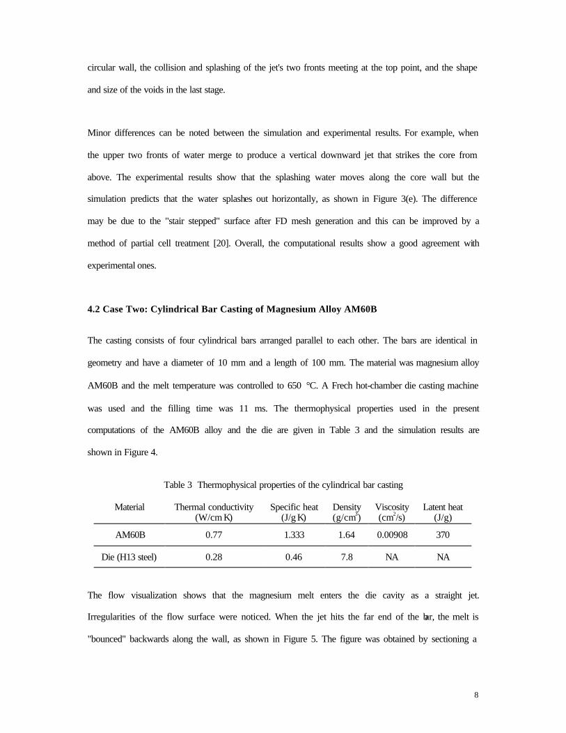
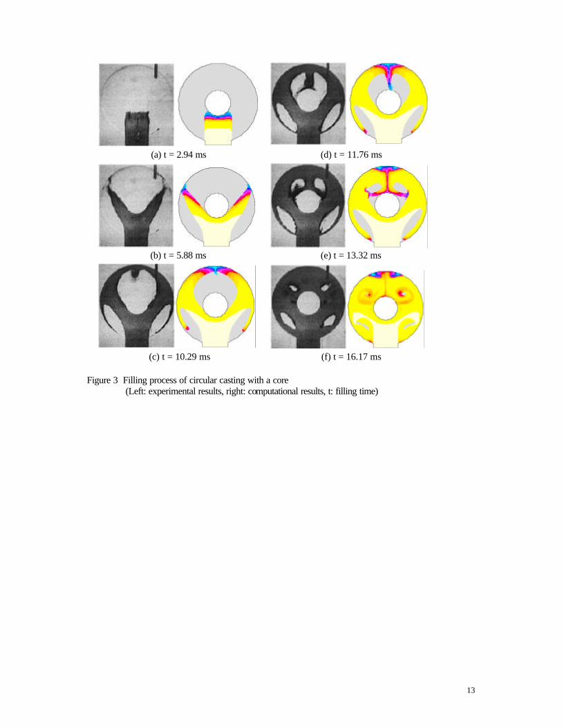
Figure 3 compares six stages of the flow of water into the die as predicted using the 3D simulation

program. The thickness in the Z direction was only 2 mm so difference in liquid temperature along Z

direction was small. Therefore, only 2D pictures are presented. Comparison of the stages in Figure 3

shows that the simulation predicts all the essential features of the flow very well. In particular, the

simulation produces reasonably accurate predictions of the shape of the jet, its trajectory along the

8

circular wall, the collision and splashing of the jet's two fronts meeting at the top point, and the shape

and size of the voids in the last stage.

Minor differences can be noted between the simulation and experimental results. For example, when

the upper two fronts of water merge to produce a vertical downward jet that strikes the core from

above. The experimental results show that the splashing water moves along the core wall but the

simulation predicts that the water splashes out horizontally, as shown in Figure 3(e). The difference

may be due to the "stair stepped" surface after FD mesh generation and this can be improved by a

method of partial cell treatment [20]. Overall, the computational results show a good agreement with

experimental ones.

4.2 Case Two: Cylindrical Bar Casting of Magnesium Alloy AM60B

The casting consists of four cylindrical bars arranged parallel to each other. The bars are identical in

geometry and have a diameter of 10 mm and a length of 100 mm. The material was magnesium alloy

AM60B and the melt temperature was controlled to 650 °C. A Frech hot-chamber die casting machine

was used and the filling time was 11 ms. The thermophysical properties used in the present

computations of the AM60B alloy and the die are given in Table 3 and the simulation results are

shown in Figure 4.

Table 3 Thermophysical properties of the cylindrical bar casting

Material Thermal conductivity (W/cm⋅K)

Specific heat (J/g⋅K)

Density (g/cm3)

Viscosity (cm2/s)

Latent heat (J/g)

AM60B 0.77 1.333 1.64 0.00908 370

Die (H13 steel) 0.28 0.46 7.8 NA NA

The flow visualization shows that the magnesium melt enters the die cavity as a straight jet.

Irregularities of the flow surface were noticed. When the jet hits the far end of the bar, the melt is

"bounced" backwards along the wall, as shown in Figure 5. The figure was obtained by sectioning a

9

bar vertically along its axis. When the melt is "bounced" back along the wall, it solidifies before the

central portion does. Therefore, the skin layer of the die-cast bar was expected to have less porosity.

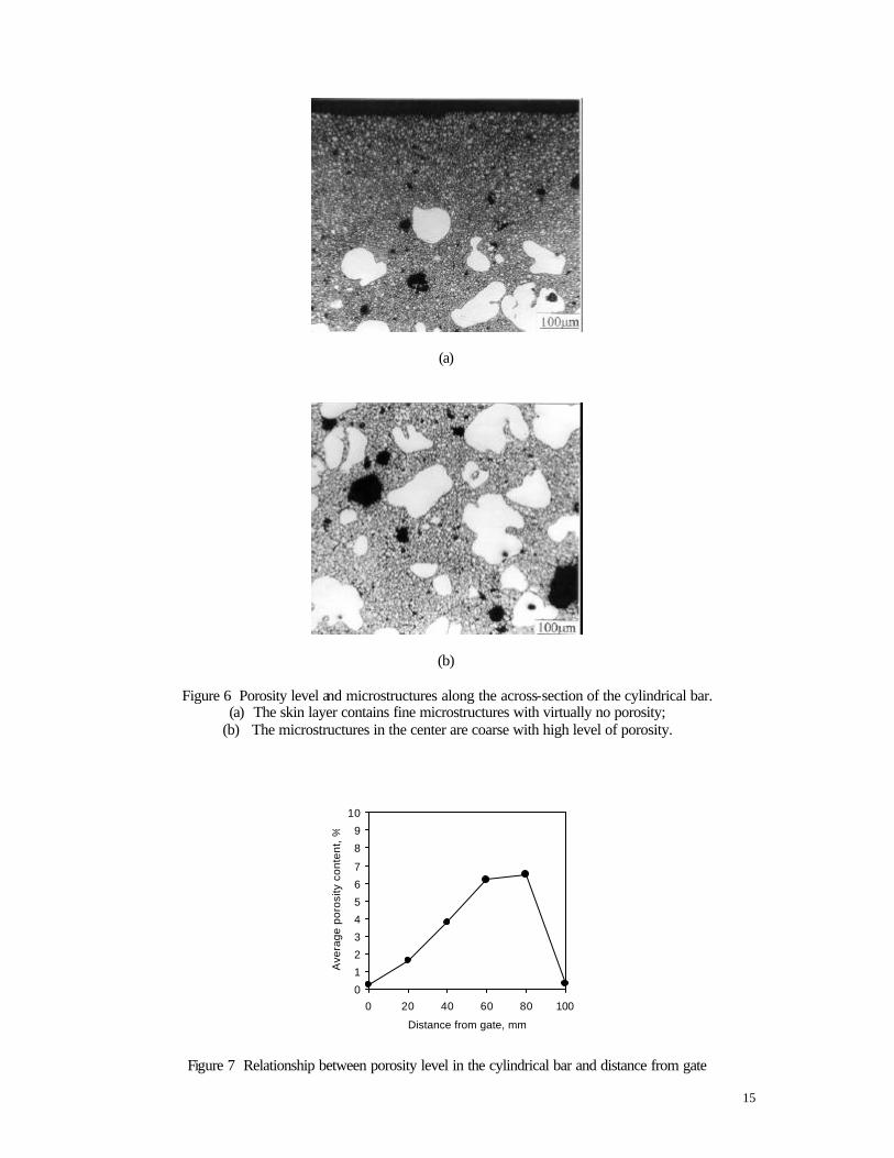
A die-cast bar was cut perpendicularly to its axis and the cross-section was ground and polished

carefully. Metallographic examination of the cross-section using a Zeiss Axiotron optical microscope

revealed that the skin layer was virtually porosity-free but the central area contained high level of

porosity, as shown in Figure 6. This confirms the above analysis. It was also be noted from Figure 6

that the skin layer consists of much finer microstructures than the core. This is because the skin

solidifies before the core and at much faster rate due to its close contact with the steel mould. The

microstructures of cast AM60B castings were observed to consist of a bi-modal distribution of α-Mg

grains and intergranular β-Mg17Al12 phases. Furthermore, α-Mg grains were surrounded by eutectic β-

Mg17Al12 phases. This structure is called a divorced eutectic [Mg(α) + Mg17Al12(β)] structure. The

formation of this divorced eutectic structure is due to the high solidification rate involved in the

magnesium die casting process.

Quantitative image analysis was performed using a Leica Quantimet 520 system on as-polished

specimens to measure the porosity contents of various cross-sections of the magnesium bar. Figure 7

shows the porosity level as a function of the distance from the gate. It was seen that the porosity level

tends to be higher at locations further away from the gate except for the extreme far end, which was

very low. This was easily understandable because it is close to the overflow slot and the mangesium

alloy solidifies early. When the overflow slot is completely filled the gas level in the melt will

determine the gas porosity in the final casting. It is known that low temperature melt tends to contain

less gas. The simulation results (see Figure 5) show that before solidification occurs the melt

temperature is higher in locations further away from the gate, and this explains well why the porosity

level is higher in locations furthest away.

10

5 Summary and Conclusions

Based on the SMAC method, the Navier-Stokes equations were solved in three dimensions by Finite

Difference Method (FDM) to simulate the filling process in die casting. The κ-ε model was used to

account for the turbulent flow during filling process. The FDM simulation program was first

examined using available experimental results for circular casting with a core. The simulated flow

patterns were found to be in good agreement with the experimental results, indicating that the free

surfaces during filling process were tracked correctly using the program. The simulation program was

further examined using experimental results for cylindrical bar die casting of an AM60B magnesium

alloy. The simulation results show that the magnesium melt enters the die cavity as a straight jet and

then "bounced" back along the wall when the jet hits the far end of the bar and that before

solidification occurs the melt temperature is higher in locations further away from the gate. These

results explain well the existence of fine-grained skin layer in the bar and the observation that porosity

level in the bar is higher in locations further away from the gate.

11

References

1. W. T. Andresen, Die Casting Engineer 41, 30 (1997).

2. G. Bar-Meir, On Gas/Air Porosity in Pressure Die Casting (Ph.D. thesis, University of Minnesota, 1995), pp. 5-9.

3. C. C. Tai and J. C. Lin, Journal of Materials Processing Technology 86, 87 (1999).

4. I. Rosindale and K. Davey, Journal of Materials Processing Technology 82, 27 (1998).

5. S. C. Lu, A. B. Rebello, R. A. Miller, G. L. Kinzel, and R. Yagel, Computer-Aided Design 29, 727 (1997).

6. M. Schmid and F. Klein, in Proceedings of 18th International Die Casting Congress and Exposition, edited by L. J. Ouimet and W. A. Bulter (North American Die Casting Association, Illinois, 1995) pp. 93-99

7. K. Anzai and T. Uchida, in Modeling of Casting, Welding and Advanced Solidification Processes V, edited by M. Rappaz, M. R. Ozgu and K. W. Mahin (Warrendale, Pa.: TMS, Switzerland, 1991), p. 741.

8. R. A. Stoehr and C. Wang, in Modeling of Casting, Welding and Advanced Solidification Processes V, edited by M. Rappaz, M. R. Ozgu and K. W. Mahin (Warrendale, Pa.: TMS, Switzerland, 1991), p. 725.

9. K. Venkatesan and R. Shivpuri, in proceedings of 18th International Die Casting Congress and Exposition, edited by L. J. Ouimet and W. A. Bulter (North American Die Casting Association, Illinois, 1995) pp. 67-73.

10. J. F. Hetu, D. M. Gao, K. K. Kabanemi, S. Bergeron, K. T. Nguyen, and C. A. Loong, Advanced Performance Materials 5, 65 (1998).

11. P. W. Cleary and J. Ha, in Proceedings of the 13th Australian Fluid Mechanics Conference, edited by W. H. Melbourne et al. (Melbourne, 1998), p. 663.

12. P. Gilotte, L. V. Huynh, J. Etay, and R. Hamar, Transactions of the ASME 117 , 82 (1995).

13. F. H. Harlow and J. E. Welch, The Physics of Fluids 8, 2182(1965).

14. W. S. Hwang and R. A. Stoehr, AFS Transactions 95, 425 (1987).

15. R. A. Stoehr, C. Wang, W. S. Hwang, and P. Ingerslev, in Modeling and Control of Casting and Welding Processes III, edited by S. Kou and R. Mehrabian (Metallurgical Society California, Warrendale, Pa., 1986), p. 303.

16. W. S. Hwang and R. A. Stoehr, Materials Science and Technology 4, 240 (1988).

17. A. A. Amsden and F. H. Harlow, Journal of Computational Physics 6, 332 (1970).

18. Y. Li and B. Liu, China Foundry Machinery & Technology 4, 46 (1998), in Chinese.

19. J. C. Tannehill, D. A. Anderson, and R. H. Pletcher, Computational Fluid Mechanics and Heat Transfer, Second Edition, (Taylor & Francis, Washington, DC, 1997), p. 314.

20. D. B. Kothe, R. C. Mjolsness, and M. D. Torrey, RIPPLE: A Computer Program for Incompressible Flows with Free Surface (Los Alamos National Laboratory, New Mexico, 1991), p. 35.

12

Start

Input data

Reflagging

Pseudopressure

Calculating tilde velocity field

Tentative divergence calculation

Over-relaxation method forpotential function

Final velocity field

Particle movement

End

Filling is over?No

Yes

Figure 1 The SMAC calculation cycle Figure 2 Dimensions of circular casting with a core (thickness =2 mm).

13

(a) t = 2.94 ms (d) t = 11.76 ms

(b) t = 5.88 ms (e) t = 13.32 ms

(c) t = 10.29 ms (f) t = 16.17 ms

Figure 3 Filling process of circular casting with a core (Left: experimental results, right: computational results, t: filling time)

14

(a)

(b)

(c)

(d)

Figure 4 Results of simulation showing filling process of cylindrical bar casting

Figure 5 Results of simulation showing that the melt enters a cylindrical bar in the form of a jet and is "bounced" backward along the wall when striking the filled part.

15

(a)

(b)

Figure 6 Porosity level and microstructures along the across-section of the cylindrical bar. (a) The skin layer contains fine microstructures with virtually no porosity;

(b) The microstructures in the center are coarse with high level of porosity.

0

1

2

3

4

5

6

7

8

9

10

0 20 40 60 80 100

Distance from gate, mm

Ave

rag

e p

oro

sity

co

nte

nt,

%

Figure 7 Relationship between porosity level in the cylindrical bar and distance from gate