Review Some Basic Statistical Concepts
55
1A.1 Copyright© 1977 John Wiley & Son, Inc. All rights reserved Review Some Basic Statistical Concept Appendix 1A
-
Upload
stacy-trujillo -
Category
Documents
-
view
59 -
download
5
description
Appendix 1A. Review Some Basic Statistical Concepts. Random Variable. random variable : A variable whose value is unknown until it is observed. The value of a random variable results from an experiment. The term random variable implies the existence of some - PowerPoint PPT Presentation
Transcript of Review Some Basic Statistical Concepts
1A.1
Copyright© 1977 John Wiley & Son, Inc. All rights reserved
Review Some Basic
Statistical Concepts
Appendix 1A
1A.2
Copyright© 1977 John Wiley & Son, Inc. All rights reserved
random variable: A variable whose value is unknown until it is observed.The value of a random variable results from an experiment.
The term random variable implies the existence of someknown or unknown probability distribution defined overthe set of all possible values of that variable.
In contrast, an arbitrary variable does not have aprobability distribution associated with its values.
Random Variable
1A.3
Copyright© 1977 John Wiley & Son, Inc. All rights reserved
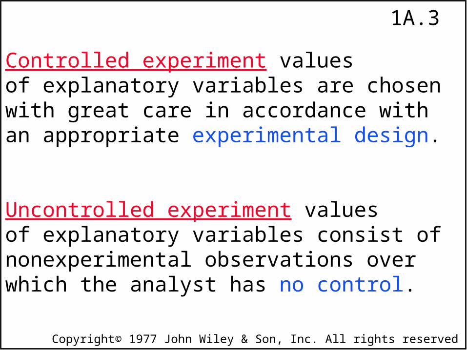
Controlled experiment values of explanatory variables are chosen with great care in accordance withan appropriate experimental design.
Uncontrolled experiment valuesof explanatory variables consist of nonexperimental observations overwhich the analyst has no control.
1A.4
Copyright© 1977 John Wiley & Son, Inc. All rights reserved
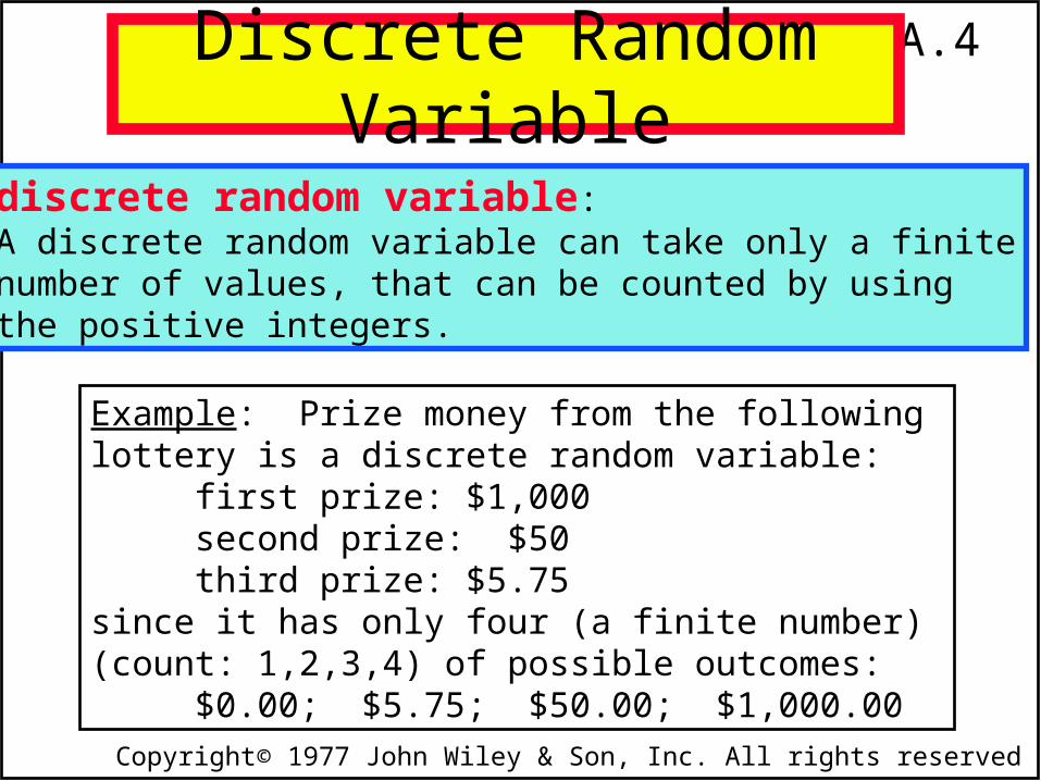
discrete random variable:A discrete random variable can take only a finitenumber of values, that can be counted by using the positive integers.
Example: Prize money from the followinglottery is a discrete random variable:
first prize: $1,000second prize: $50third prize: $5.75
since it has only four (a finite number) (count: 1,2,3,4) of possible outcomes:
$0.00; $5.75; $50.00; $1,000.00
Discrete Random Variable
1A.5
Copyright© 1977 John Wiley & Son, Inc. All rights reserved
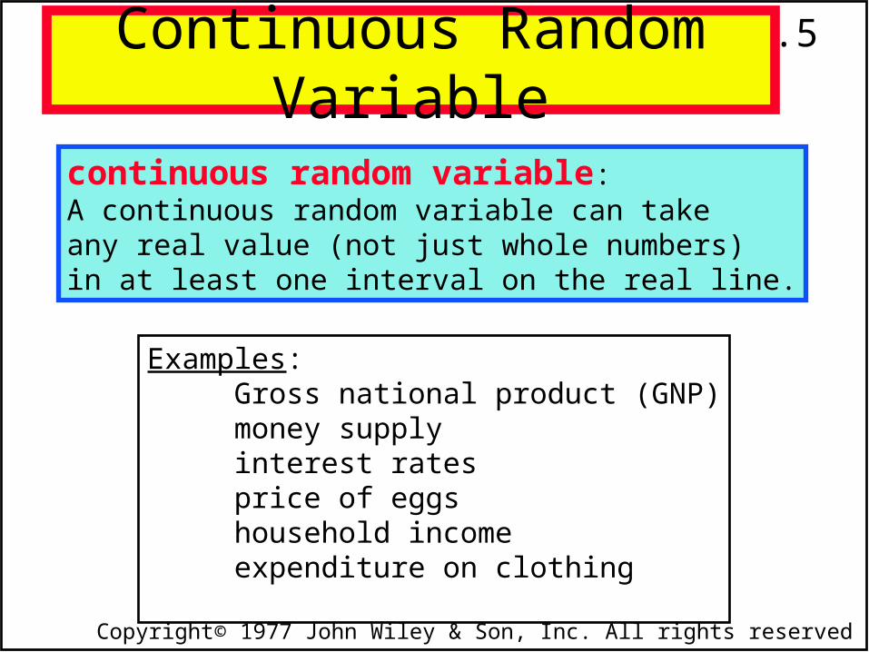
continuous random variable:A continuous random variable can take any real value (not just whole numbers) in at least one interval on the real line.
Examples: Gross national product (GNP)money supplyinterest ratesprice of eggshousehold incomeexpenditure on clothing
Continuous Random Variable
1A.6
Copyright© 1977 John Wiley & Son, Inc. All rights reserved
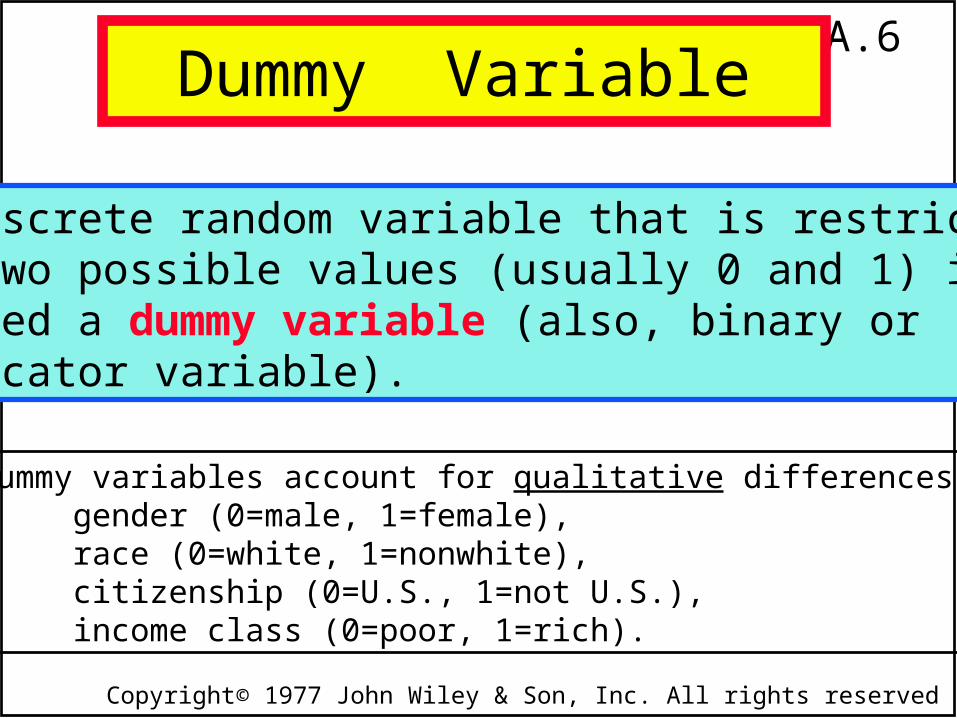
A discrete random variable that is restrictedto two possible values (usually 0 and 1) iscalled a dummy variable (also, binary orindicator variable).
Dummy variables account for qualitative differences:gender (0=male, 1=female), race (0=white, 1=nonwhite),citizenship (0=U.S., 1=not U.S.), income class (0=poor, 1=rich).
Dummy Variable
1A.7
Copyright© 1977 John Wiley & Son, Inc. All rights reserved
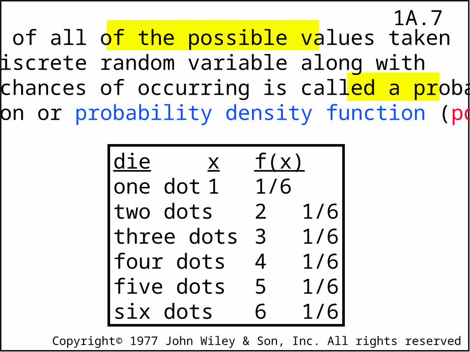
A list of all of the possible values takenby a discrete random variable along withtheir chances of occurring is called a probabilityfunction or probability density function (pdf).
die x f(x)one dot 1 1/6two dots 2 1/6three dots 3 1/6four dots 4 1/6five dots 5 1/6six dots 6 1/6
1A.8
Copyright© 1977 John Wiley & Son, Inc. All rights reserved
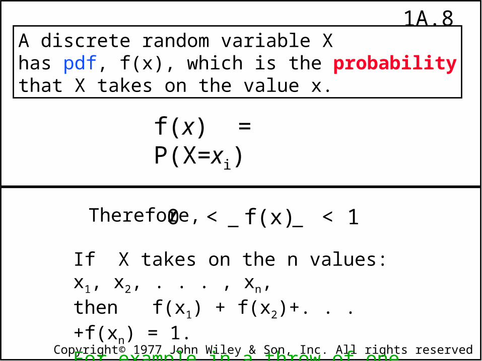
A discrete random variable X has pdf, f(x), which is the probabilitythat X takes on the value x.
f(x) = P(X=xi)
0 < f(x) < 1
If X takes on the n values: x1, x2, . . . , xn, then f(x1) + f(x2)+. . .+f(xn) = 1.For example in a throw of one dice:(1/6) + (1/6) + (1/6) + (1/6) + (1/6) + (1/6)=1
Therefore,
1A.9
Copyright© 1977 John Wiley & Son, Inc. All rights reserved
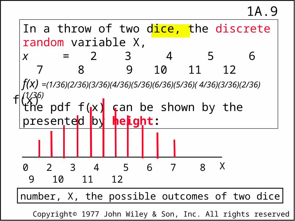
In a throw of two dice, the discrete random variable X,x = 2 3 4 5 6 7 8 9 10 11 12f(x) =(1/36)(2/36)(3/36)(4/36)(5/36)(6/36)(5/36)( 4/36)(3/36)(2/36)(1/36)
the pdf f(x) can be shown by the presented by height:
0 2 3 4 5 6 7 8 9 10 11 12 X
number, X, the possible outcomes of two dice
f(x)
1A.10
Copyright© 1977 John Wiley & Son, Inc. All rights reserved
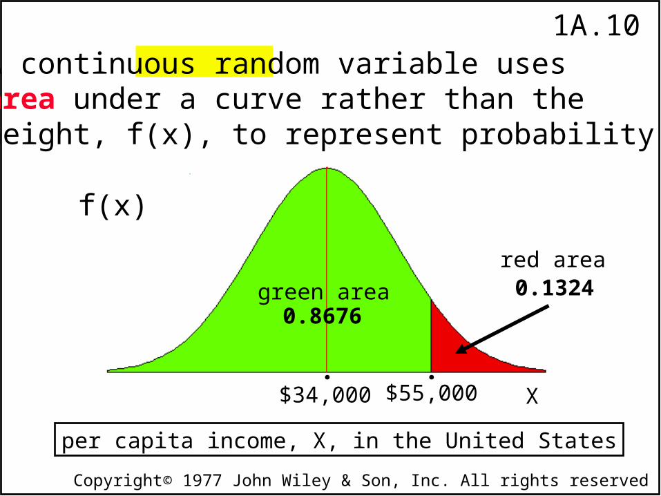
A continuous random variable uses area under a curve rather than theheight, f(x), to represent probability:
f(x)
X$34,000 $55,000. .
per capita income, X, in the United States
0.13240.8676
red area
green area
1A.11
Copyright© 1977 John Wiley & Son, Inc. All rights reserved
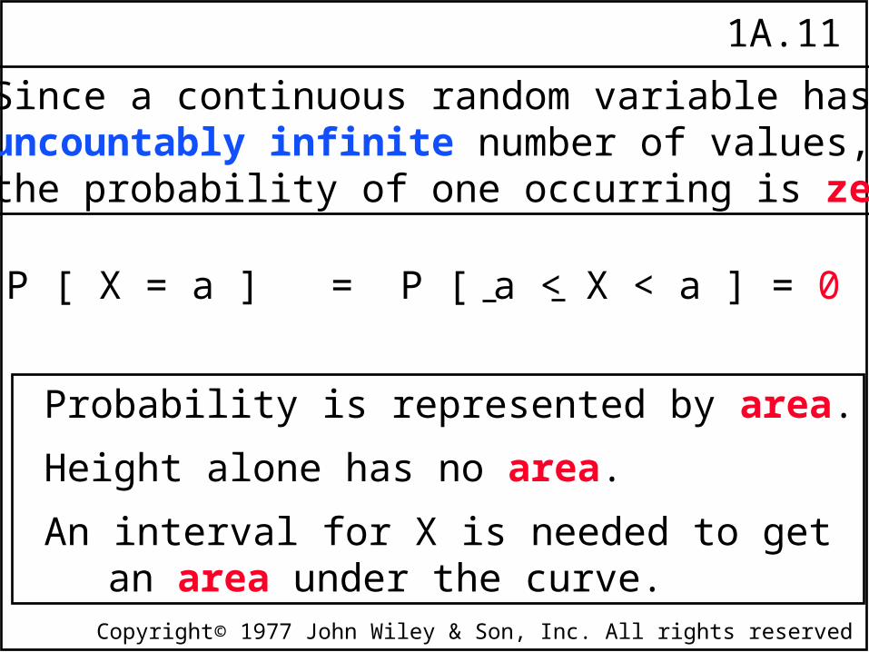
Since a continuous random variable has an uncountably infinite number of values, the probability of one occurring is zero.
P [ X = a ] = P [ a < X < a ] = 0
Probability is represented by area.
Height alone has no area.
An interval for X is needed to get an area under the curve.
1A.12
Copyright© 1977 John Wiley & Son, Inc. All rights reserved
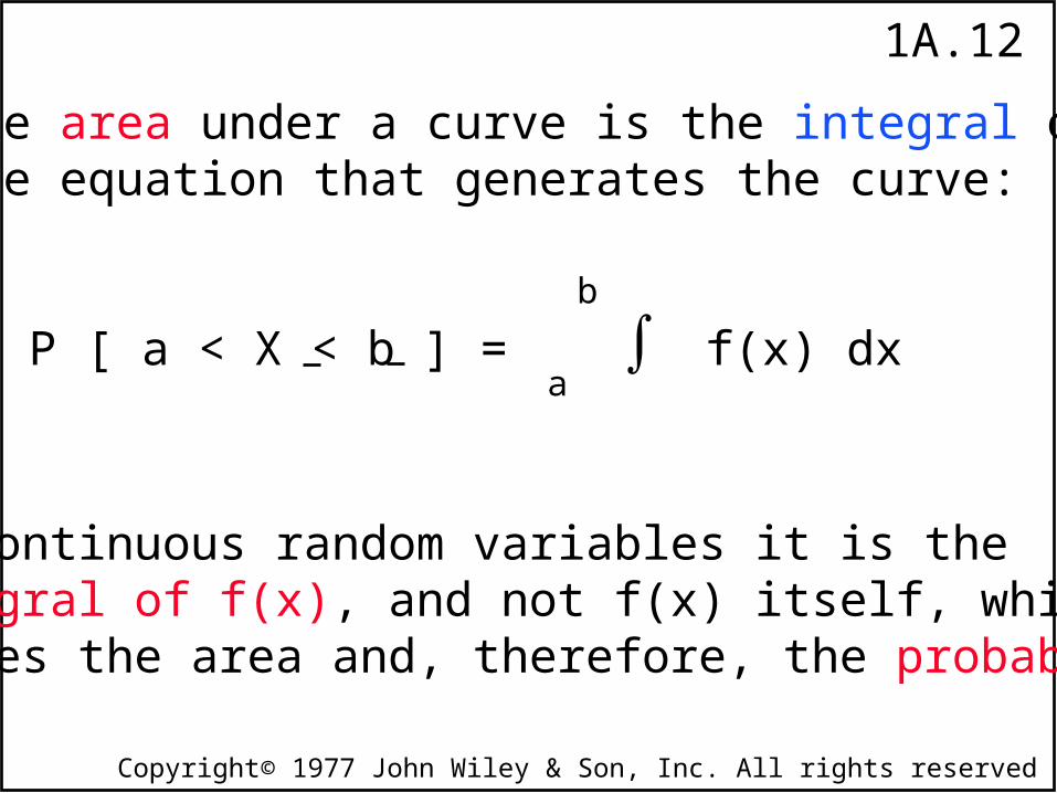
P [ a < X < b ] = f(x) dxb
a
The area under a curve is the integral ofthe equation that generates the curve:
For continuous random variables it is the integral of f(x), and not f(x) itself, whichdefines the area and, therefore, the probability.
1A.13
Copyright© 1977 John Wiley & Son, Inc. All rights reserved
n
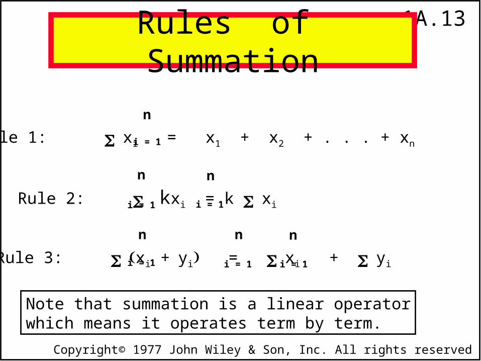
Rule 2: kxi = k xi i = 1 i = 1
n
Rule 1: xi = x1 + x2 + . . . + xni = 1
n
Rule 3: xi +yi = xi + yii = 1 i = 1 i = 1
n n n
Note that summation is a linear operatorwhich means it operates term by term.
Rules of Summation
1A.14
Copyright© 1977 John Wiley & Son, Inc. All rights reserved
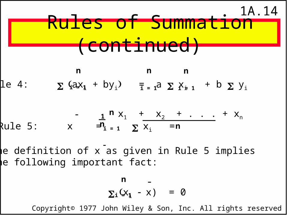
Rule 4: axi +byi = a xi + b yii = 1 i = 1 i = 1
n n n
Rules of Summation (continued)
Rule 5: x = xi =i = 1
n
n1 x1 + x2 + . . . + xn
n
The definition of x as given in Rule 5 impliesthe following important fact:
xi x) = 0i = 1
n
1A.15
Copyright© 1977 John Wiley & Son, Inc. All rights reserved
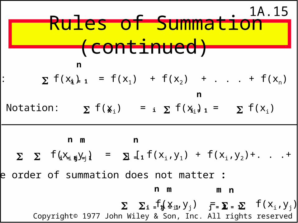
Rule 6: f(xi) = f(x1) + f(x2) + . . . + f(xn)i = 1
n
Notation: f(xi) = f(xi) = f(xi)
n
x i i = 1
n
Rule 7: f(xi,yj) = [ f(xi,y1) + f(xi,y2)+. . .+ f(xi,ym)] i = 1 i = 1
n m
j = 1
The order of summation does not matter :
f(xi,yj) = f(xi,yj)i = 1
n m
j = 1 j = 1
m n
i = 1
Rules of Summation (continued)
1A.16
Copyright© 1977 John Wiley & Son, Inc. All rights reserved
The mean or arithmetic average of arandom variable is its mathematicalexpectation or expected value, E(X).
The Mean of a Random Variable
1A.17
Copyright© 1977 John Wiley & Son, Inc. All rights reserved
Expected Value
There are two entirely different, but mathematicallyequivalent, ways of determining the expected value:
1. Empirically: The expected value of a random variable, X,is the average value of the random variable in aninfinite number of repetitions of the experiment.
In other words, draw an infinite number of samples,and average the values of X that you get.
1A.18
Copyright© 1977 John Wiley & Son, Inc. All rights reserved
Expected Value
2. Analytically: The expected value of a discrete random variable, X, is determined by weighting all the possible values of X by the correspondingprobability density function values, f(x), and summing them up.
E(X) = x1f(x1) + x2f(x2) + . . . + xnf(xn)
In other words:
1A.19
Copyright© 1977 John Wiley & Son, Inc. All rights reserved
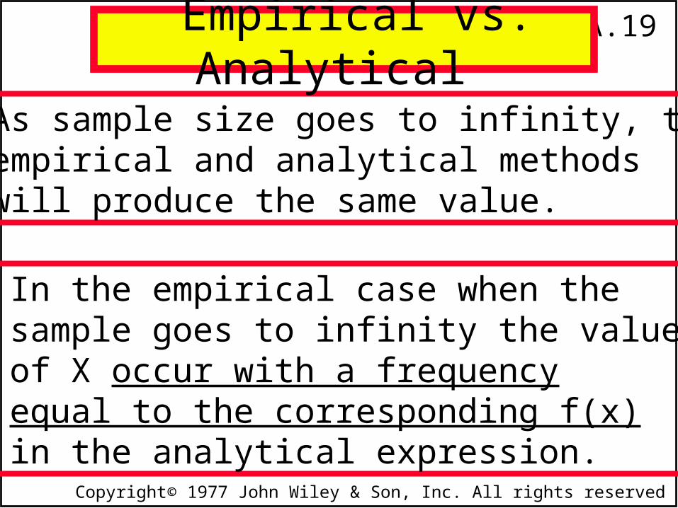
In the empirical case when the sample goes to infinity the values of X occur with a frequency equal to the corresponding f(x) in the analytical expression.
As sample size goes to infinity, the empirical and analytical methods will produce the same value.
Empirical vs. Analytical
1A.20
Copyright© 1977 John Wiley & Son, Inc. All rights reserved
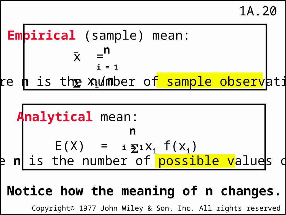
x = xi/nn
i = 1
where n is the number of sample observations.
Empirical (sample) mean:
E(X) = xif(xi)i = 1
n
where n is the number of possible values of xi.
Analytical mean:
Notice how the meaning of n changes.
1A.21
Copyright© 1977 John Wiley & Son, Inc. All rights reserved
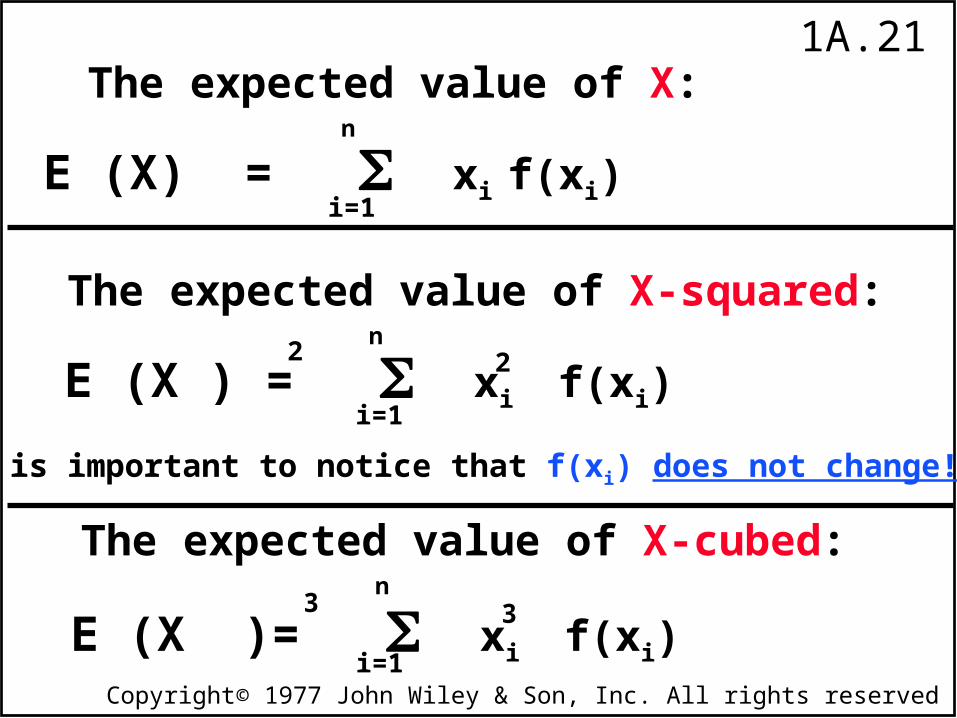
E (X) = xi f(xi) i=1
n
The expected value of X-squared:
E (X ) = xi f(xi) i=1
n 2 2
It is important to notice that f(xi) does not change!
The expected value of X-cubed:
E (X )= xi f(xi) i=1
n 3 3
The expected value of X:
1A.22
Copyright© 1977 John Wiley & Son, Inc. All rights reserved
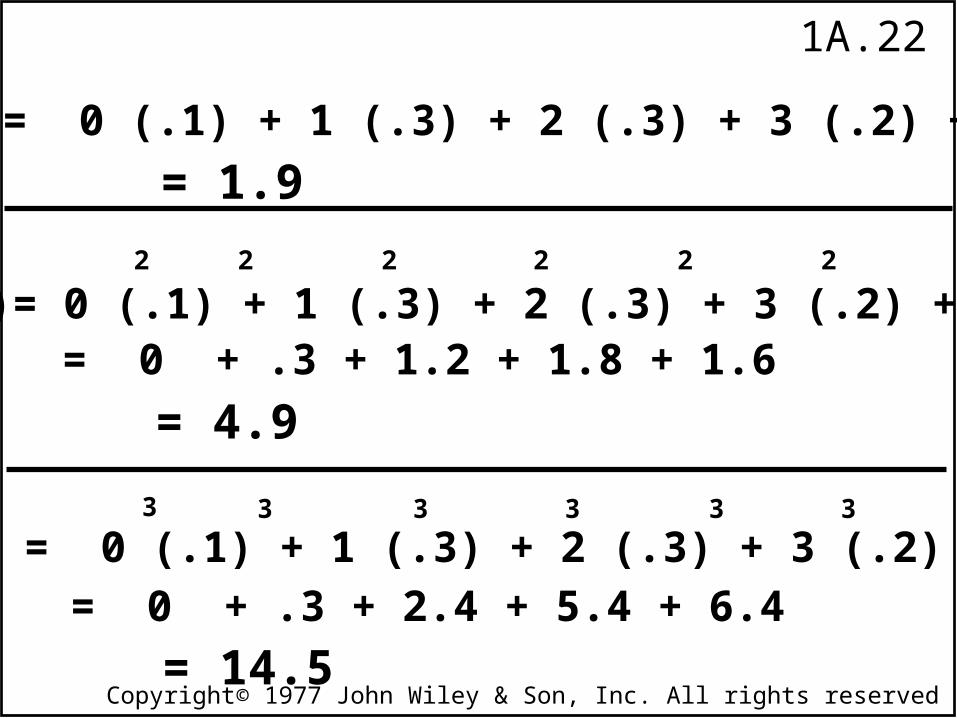
E(X) = 0 (.1) + 1 (.3) + 2 (.3) + 3 (.2) + 4 (.1)
2
E(X )= 0 (.1) + 1 (.3) + 2 (.3) + 3 (.2) + 4 (.1)22222
= 1.9
= 0 + .3 + 1.2 + 1.8 + 1.6
= 4.9
3
E( X ) = 0 (.1) + 1 (.3) + 2 (.3) + 3 (.2) +4 (.1) 3 3 3 3 3
= 0 + .3 + 2.4 + 5.4 + 6.4
= 14.5
1A.23
Copyright© 1977 John Wiley & Son, Inc. All rights reserved
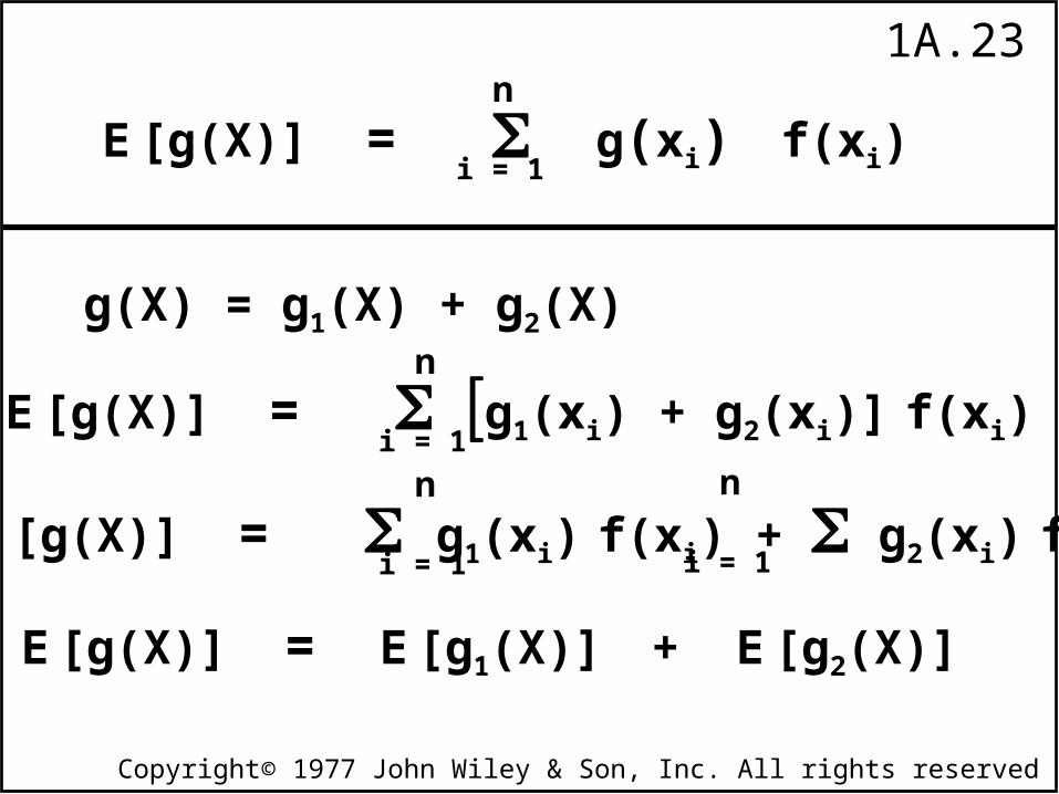
E [g(X)] = g(xi) f(xi)n
i = 1
g(X) = g1(X) + g2(X)
E [g(X)] = g1(xi) + g2(xi)] f(xi)n
i = 1
E [g(X)] = g1(xi) f(xi) + g2(xi) f(xi)n
i = 1
n
i = 1
E [g(X)] = E [g1(X)] + E [g2(X)]
1A.24
Copyright© 1977 John Wiley & Son, Inc. All rights reserved
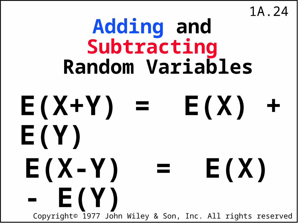
Adding and Subtracting Random Variables
E(X-Y) = E(X) - E(Y)
E(X+Y) = E(X) + E(Y)
1A.25
Copyright© 1977 John Wiley & Son, Inc. All rights reserved
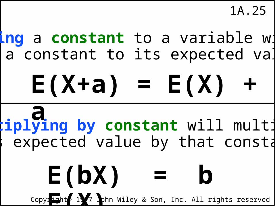
E(X+a) = E(X) + a
Adding a constant to a variable willadd a constant to its expected value:
Multiplying by constant will multiply its expected value by that constant:
E(bX) = b E(X)
1A.26
Copyright© 1977 John Wiley & Son, Inc. All rights reserved
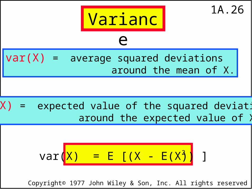
var(X) = average squared deviations around the mean of X.
var(X) = expected value of the squared deviations around the expected value of X.
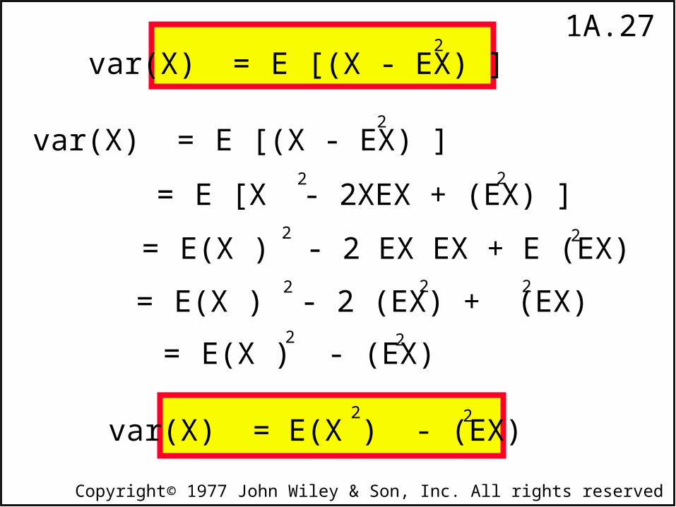
var(X) = E [(X - E(X)) ] 2
Variance
1A.27
Copyright© 1977 John Wiley & Son, Inc. All rights reserved
var(X) = E [(X - EX) ]
= E [X - 2XEX + (EX) ]
2
2
2= E(X ) - 2 EX EX + E (EX)
2
2
= E(X ) - 2 (EX) + (EX) 2 2 2
= E(X ) - (EX) 2 2
var(X) = E [(X - EX) ] 2
var(X) = E(X ) - (EX) 22
1A.28
Copyright© 1977 John Wiley & Son, Inc. All rights reserved
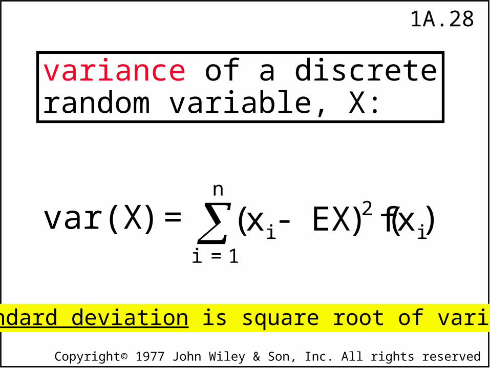
variance of a discreterandom variable, X:
standard deviation is square root of variance
var ( X ) = (xi - EX )2 f(xi)i = 1
n
1A.29
Copyright© 1977 John Wiley & Son, Inc. All rights reserved
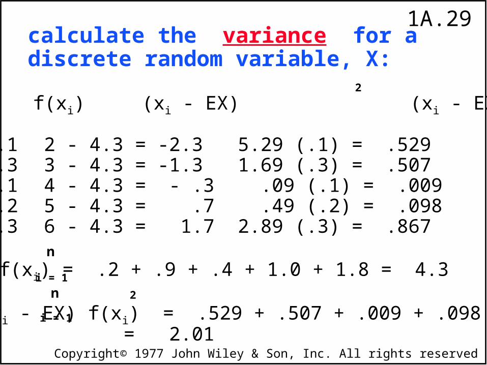
xi f(xi) (xi - EX) (xi - EX) f(xi)
2 .1 2 - 4.3 = -2.3 5.29 (.1) = .5293 .3 3 - 4.3 = -1.3 1.69 (.3) = .5074 .1 4 - 4.3 = - .3 .09 (.1) = .0095 .2 5 - 4.3 = .7 .49 (.2) = .0986 .3 6 - 4.3 = 1.7 2.89 (.3) = .867
xi f(xi) = .2 + .9 + .4 + 1.0 + 1.8 = 4.3
(xi - EX) f(xi) = .529 + .507 + .009 + .098 + .867 = 2.01
2
2
calculate the variance for a discrete random variable, X:
i = 1
n
n
i = 1
1A.30
Copyright© 1977 John Wiley & Son, Inc. All rights reserved
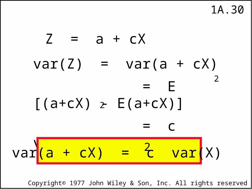
Z = a + cX
var(Z) = var(a + cX)
= E [(a+cX) - E(a+cX)]
= c var(X)
2
2
var(a + cX) = c var(X)2
1A.31
Copyright© 1977 John Wiley & Son, Inc. All rights reserved
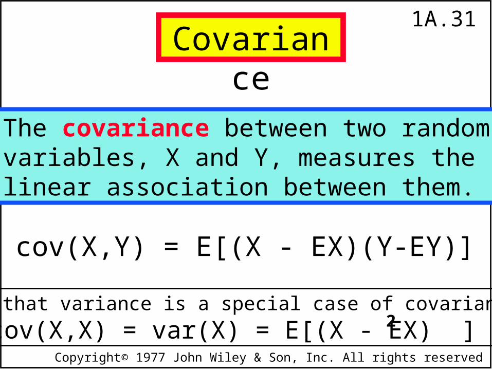
The covariance between two randomvariables, X and Y, measures thelinear association between them.
cov(X,Y) = E[(X - EX)(Y-EY)]
Note that variance is a special case of covariance.
cov(X,X) = var(X) = E[(X - EX) ]2
Covariance
1A.32
Copyright© 1977 John Wiley & Son, Inc. All rights reserved
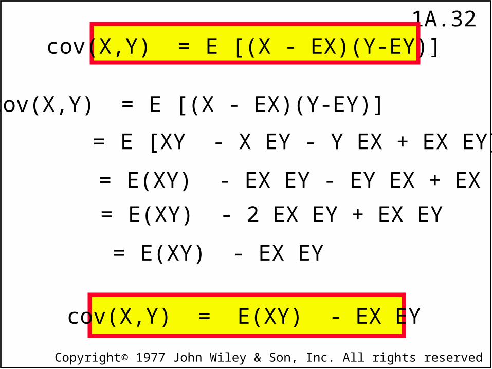
cov(X,Y) = E [(X - EX)(Y-EY)]
= E [XY - X EY - Y EX + EX EY]
= E(XY) - 2 EX EY + EX EY
= E(XY) - EX EY
cov(X,Y) = E [(X - EX)(Y-EY)]
cov(X,Y) = E(XY) - EX EY
= E(XY) - EX EY - EY EX + EX EY
1A.33
Copyright© 1977 John Wiley & Son, Inc. All rights reserved
.15
.05
.45
.35
Y = 1 Y = 2
X = 0
X = 1
.60
.40
.50.50
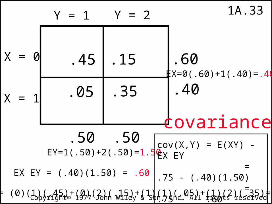
EX=0(.60)+1(.40)=.40
EY=1(.50)+2(.50)=1.50
E(XY) = (0)(1)(.45)+(0)(2)(.15)+(1)(1)(.05)+(1)(2)(.35)=.75
EX EY = (.40)(1.50) = .60
cov(X,Y) = E(XY) - EX EY = .75 - (.40)(1.50) = .75 - .60 = .15
covariance
1A.34
Copyright© 1977 John Wiley & Son, Inc. All rights reserved
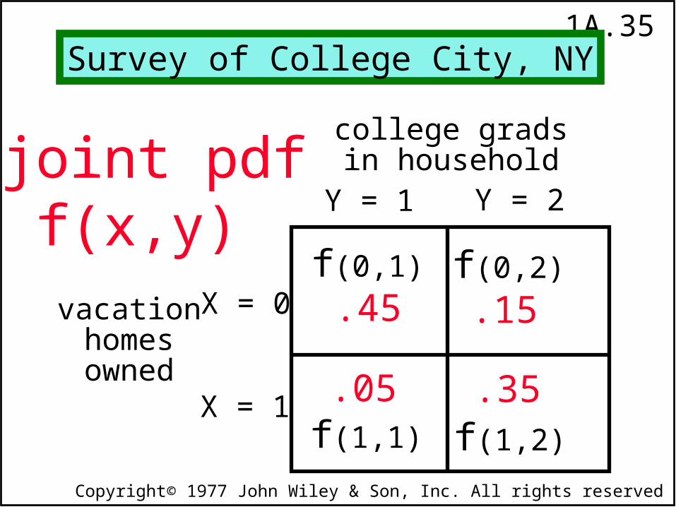
A joint probability density function, f(x,y), provides the probabilities associated with the joint occurrence of all of the possible pairs of X and Y.
Joint pdf
1A.35
Copyright© 1977 John Wiley & Son, Inc. All rights reserved
college gradsin household
.15
.05
.45
.35
joint pdff(x,y)
Y = 1 Y = 2
vacationhomesowned
X = 0
X = 1
Survey of College City, NY
f(0,1) f(0,2)
f(1,1) f(1,2)
1A.36
Copyright© 1977 John Wiley & Son, Inc. All rights reserved
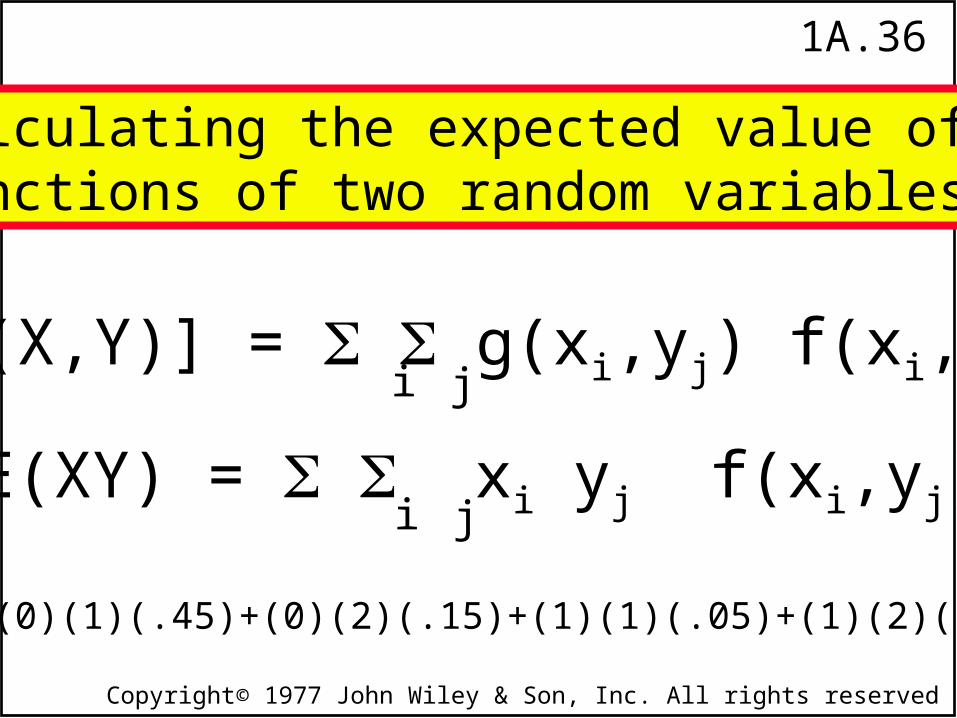
E[g(X,Y)] = g(xi,yj) f(xi,yj)i j
E(XY) = (0)(1)(.45)+(0)(2)(.15)+(1)(1)(.05)+(1)(2)(.35)=.75
E(XY) = xi yj f(xi,yj)i j
Calculating the expected value of functions of two random variables.
1A.37
Copyright© 1977 John Wiley & Son, Inc. All rights reserved
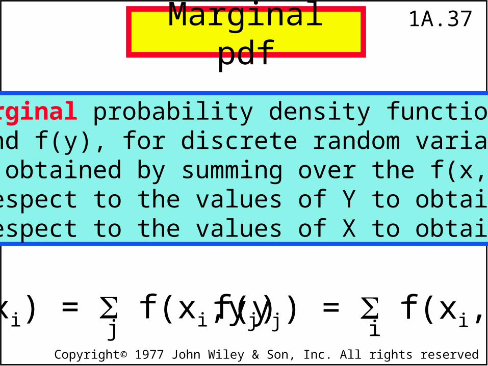
The marginal probability density functions,f(x) and f(y), for discrete random variables,can be obtained by summing over the f(x,y) with respect to the values of Y to obtain f(x) with respect to the values of X to obtain f(y).
f(xi) = f(xi,yj) f(yj) = f(xi,yj)ij
Marginal pdf
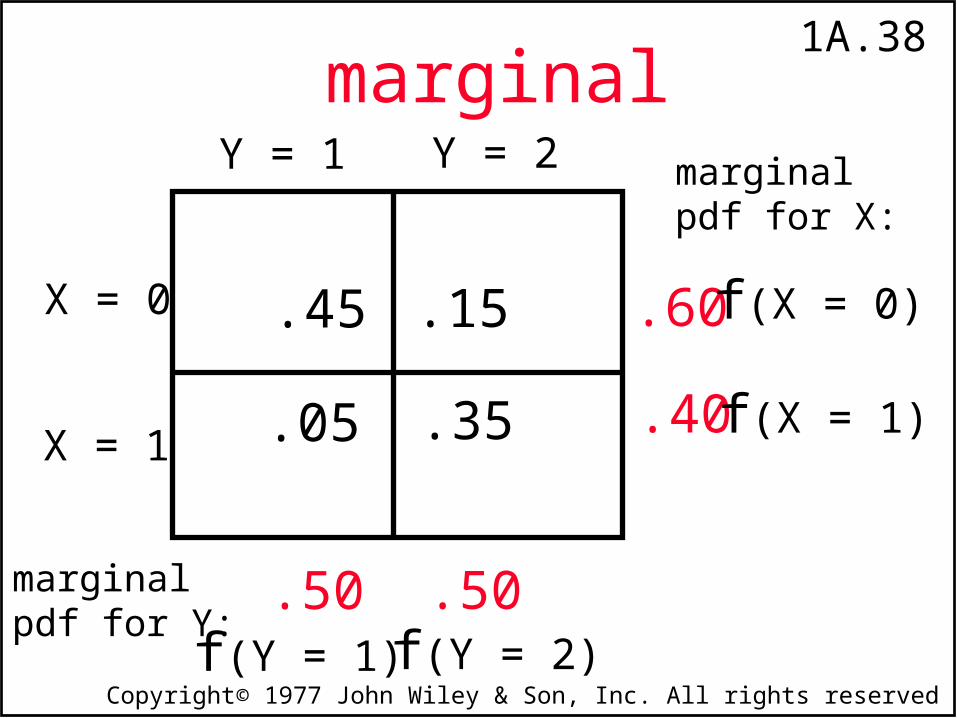
1A.38
Copyright© 1977 John Wiley & Son, Inc. All rights reserved
.15
.05
.45
.35
marginalY = 1 Y = 2
X = 0
X = 1
.60
.40
.50.50
f(X = 1)
f(X = 0)
f(Y = 1) f(Y = 2)
marginalpdf for Y:
marginalpdf for X:
1A.39
Copyright© 1977 John Wiley & Son, Inc. All rights reserved
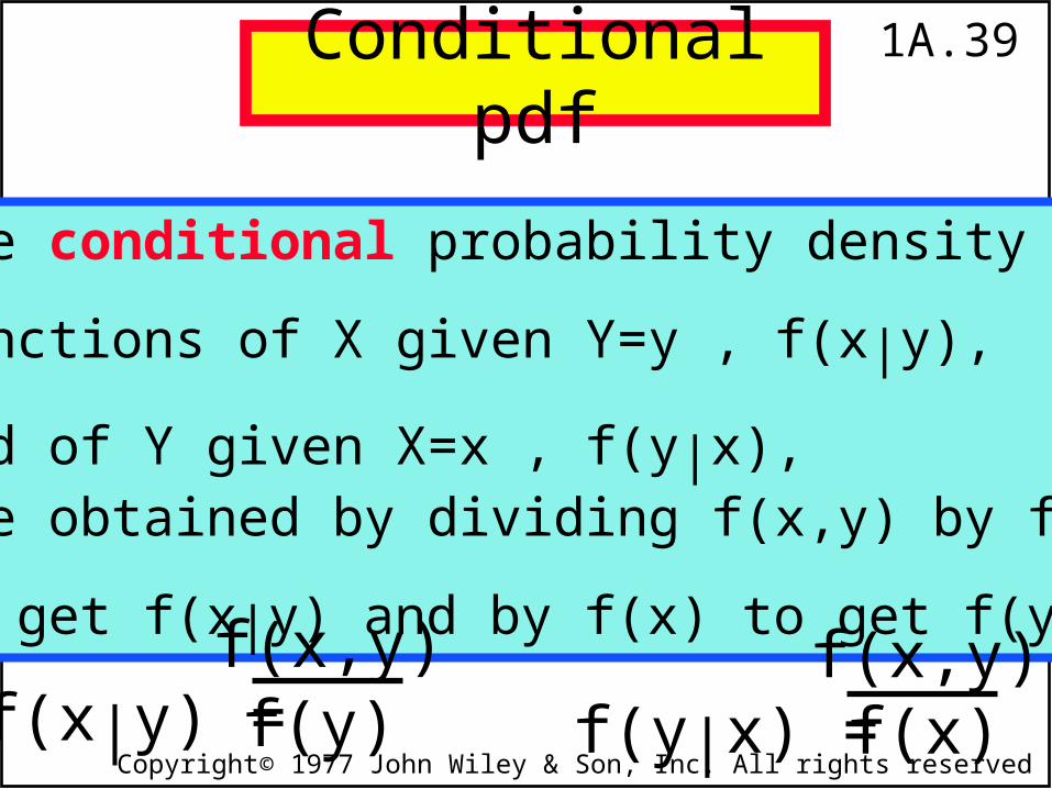
The conditional probability density
functions of X given Y=y , f(x|y),
and of Y given X=x , f(y|x), are obtained by dividing f(x,y) by f(y)
to get f(x|y) and by f(x) to get f(y|x).
f(x|y) = f(y|x) =f(x,y) f(x,y)f(y) f(x)
Conditional pdf
1A.40
Copyright© 1977 John Wiley & Son, Inc. All rights reserved
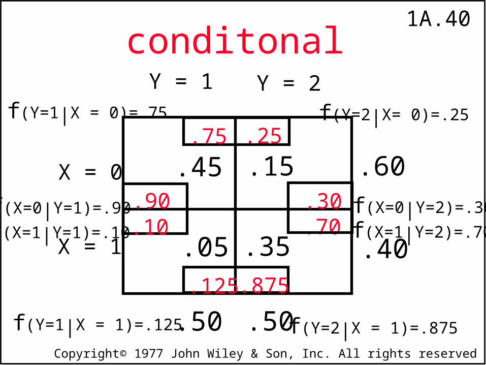
.15
.05
.45
.35
conditonalY = 1 Y = 2
X = 0
X = 1
.60
.40
.50.50
.25.75
.875.125
.90.10 .70
.30
f(Y=2|X= 0)=.25f(Y=1|X = 0)=.75
f(Y=2|X = 1)=.875
f(X=0|Y=2)=.30
f(X=1|Y=2)=.70
f(X=0|Y=1)=.90
f(X=1|Y=1)=.10
f(Y=1|X = 1)=.125
1A.41
Copyright© 1977 John Wiley & Son, Inc. All rights reserved
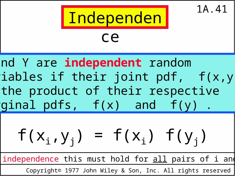
X and Y are independent random variables if their joint pdf, f(x,y),is the product of their respectivemarginal pdfs, f(x) and f(y) .
f(xi,yj) = f(xi) f(yj)for independence this must hold for all pairs of i and j
Independence
1A.42
Copyright© 1977 John Wiley & Son, Inc. All rights reserved
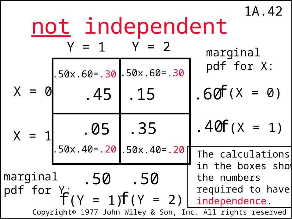
.15
.05
.45
.35
not independentY = 1 Y = 2
X = 0
X = 1
.60
.40
.50.50
f(X = 1)
f(X = 0)
f(Y = 1) f(Y = 2)
marginalpdf for Y:
marginalpdf for X:
.50x.60=.30 .50x.60=.30
.50x.40=.20 .50x.40=.20 The calculations in the boxes show the numbers required to have independence.
1A.43
Copyright© 1977 John Wiley & Son, Inc. All rights reserved
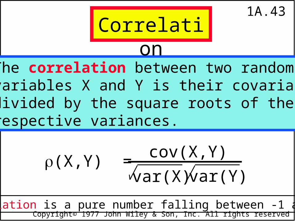
The correlation between two random variables X and Y is their covariance divided by the square roots of their respective variances.
Correlation is a pure number falling between -1 and 1.
cov(X,Y)(X,Y) =var(X) var(Y)
Correlation
1A.44
Copyright© 1977 John Wiley & Son, Inc. All rights reserved
.15
.05
.45
.35
Y = 1 Y = 2
X = 0
X = 1
.60
.40
.50.50
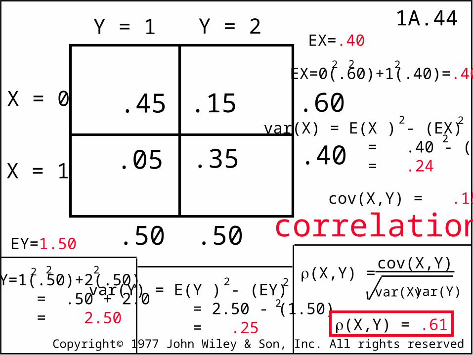
EX=.40
EY=1.50
cov(X,Y) = .15
correlation
EX=0(.60)+1(.40)=.4022 2
var(X) = E(X ) - (EX) = .40 - (.40) = .24
2 2
2
EY=1(.50)+2(.50) = .50 + 2.0 = 2.50
2 2 2
var(Y) = E(Y ) - (EY) = 2.50 - (1.50) = .25
2 2
2
(X,Y) =cov(X,Y)
var(X) var(Y)
(X,Y) = .61
1A.45
Copyright© 1977 John Wiley & Son, Inc. All rights reserved
Independent random variables have zero covariance and, therefore, zero correlation.
The converse is not true.
Zero Covariance & Correlation
1A.46
Copyright© 1977 John Wiley & Son, Inc. All rights reserved
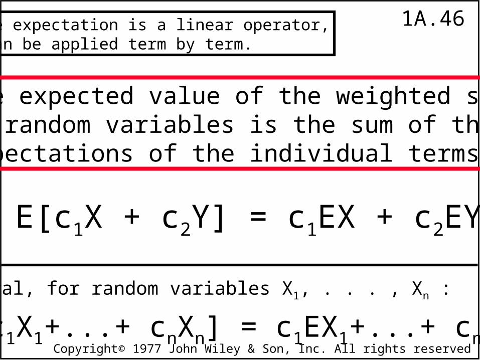
The expected value of the weighted sumof random variables is the sum of the expectations of the individual terms.
Since expectation is a linear operator,it can be applied term by term.
E[c1X + c2Y] = c1EX + c2EY
E[c1X1+...+ cnXn] = c1EX1+...+ cnEXn
In general, for random variables X1, . . . , Xn :
1A.47
Copyright© 1977 John Wiley & Son, Inc. All rights reserved
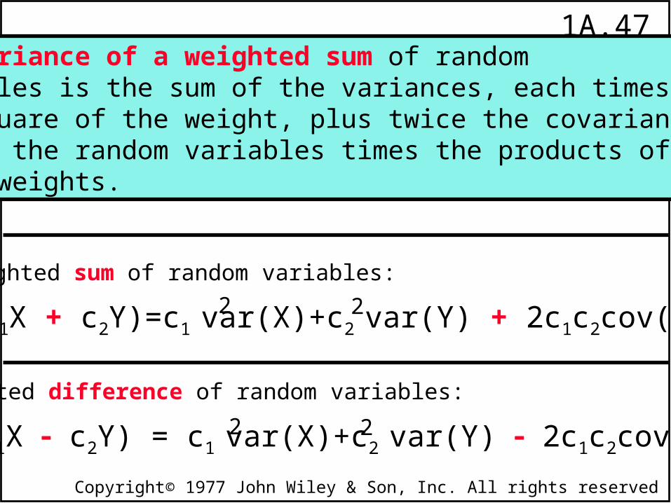
The variance of a weighted sum of random variables is the sum of the variances, each times the square of the weight, plus twice the covariances of all the random variables times the products of their weights.
var(c1X + c2Y)=c1 var(X)+c2 var(Y) + 2c1c2cov(X,Y)2 2
var(c1X c2Y) = c1 var(X)+c2 var(Y) 2c1c2cov(X,Y)2 2
Weighted sum of random variables:
Weighted difference of random variables:
1A.48
Copyright© 1977 John Wiley & Son, Inc. All rights reserved
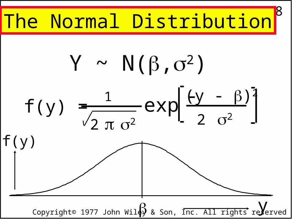
The Normal Distribution
Y ~ N(,2)
f(y) =2 2
1 exp
y
f(y)
2 2
(y - )2-
1A.49
Copyright© 1977 John Wiley & Son, Inc. All rights reserved
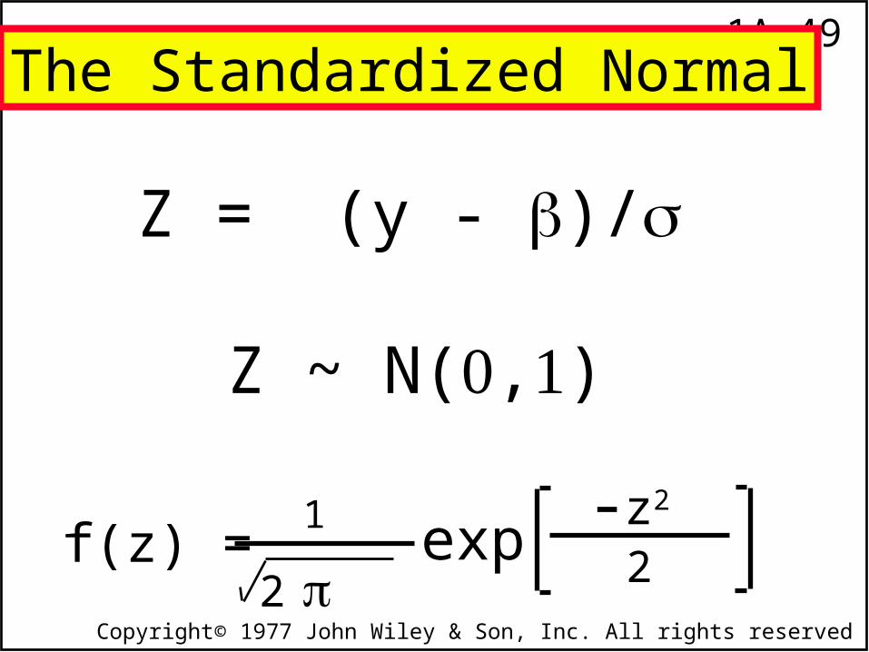
The Standardized Normal
Z ~ N(,)
f(z) =2
1 exp 2z2-
Z = (y - )/
1A.50
Copyright© 1977 John Wiley & Son, Inc. All rights reserved
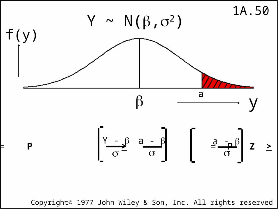
P [ Y > a ] = P > = P Z > a - a - Y -
y
f(y)
a
Y ~ N(,2)
1A.51
Copyright© 1977 John Wiley & Son, Inc. All rights reserved
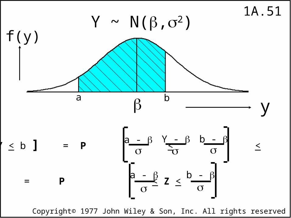
P [ a < Y < b ] = P < <
= P < Z <
a - Y -
b -
a -
b -
y
f(y)
a
Y ~ N(,2)
b
1A.52
Copyright© 1977 John Wiley & Son, Inc. All rights reserved
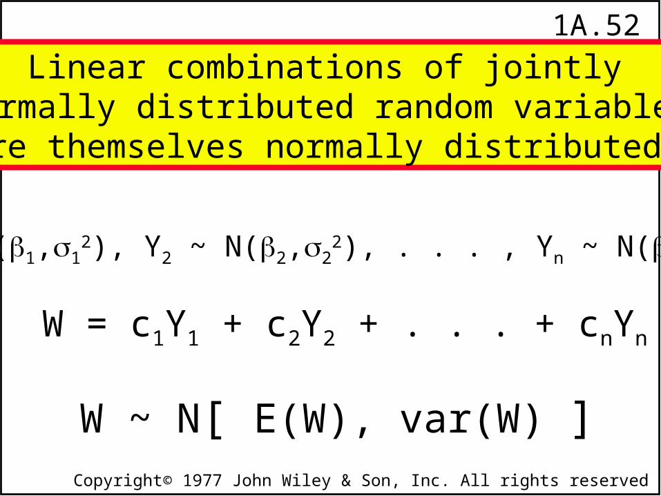
Y1 ~ N(1,12), Y2 ~ N(2,2
2), . . . , Yn ~ N(n,n2)
W = c1Y1 + c2Y2 + . . . + cnYn
Linear combinations of jointlynormally distributed random variablesare themselves normally distributed.
W ~ N[ E(W), var(W) ]
1A.53
Copyright© 1977 John Wiley & Son, Inc. All rights reserved
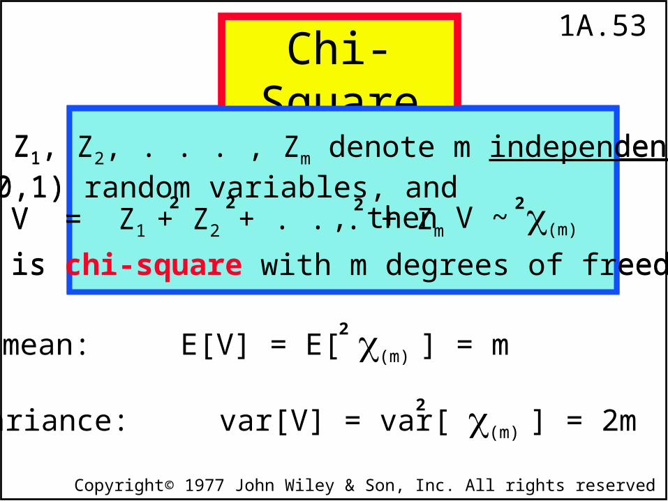
mean: E[V] = E[ (m) ] = m
If Z1, Z2, . . . , Zm denote m independentN(0,1) random variables, andV = Z1 + Z2 + . . . + Zm , then V ~ (m)
2 2 2 2
V is chi-square with m degrees of freedom.
Chi-Square
variance: var[V] = var[ (m) ] = 2m
If Z1, Z2, . . . , Zm denote m independentN(0,1) random variables, andV = Z1 + Z2 + . . . + Zm , then V ~ (m)
2 2 2 2
V is chi-square with m degrees of freedom.
2
2
1A.54
Copyright© 1977 John Wiley & Son, Inc. All rights reserved
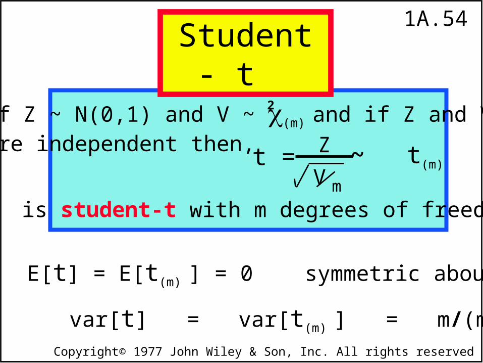
mean: E[t] = E[t(m) ] = 0 symmetric about zero
variance: var[t] = var[t(m) ] = m/(m-2)
If Z ~ N(0,1) and V ~ (m) and if Z and Vare independent then, ~ t(m)
t is student-t with m degrees of freedom.
2
t = Z
V m
Student - t
1A.55
Copyright© 1977 John Wiley & Son, Inc. All rights reserved
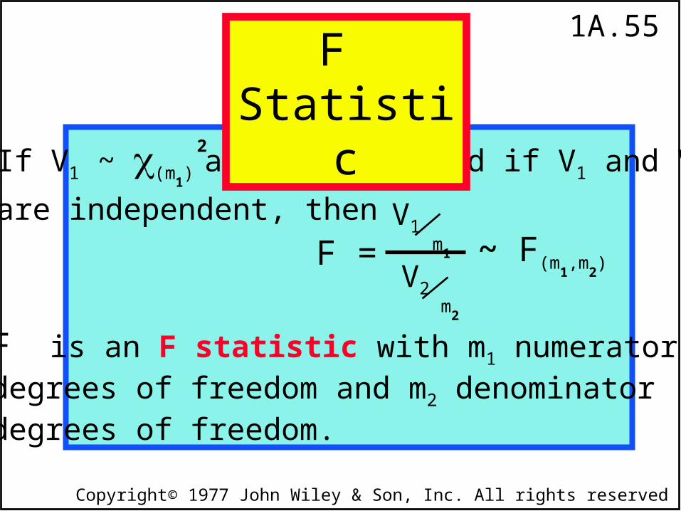
If V1 ~ (m1) and V2 ~ (m
2) and if V1 and V2
are independent, then~ F(m
1,m
2)
F is an F statistic with m1 numeratordegrees of freedom and m2 denominatordegrees of freedom.
2
F =V1
m1
V2m
2
2
F Statistic