Review on Probability Distributions (Chapters 5 & 6)slrace/aa591/CHapter 5and6_LectureNotes.pdf ·...
50
1 Slide © 2007 Thomson South - Western. All Rights Reserved Review on Probability Distributions (Chapters 5 & 6)
Transcript of Review on Probability Distributions (Chapters 5 & 6)slrace/aa591/CHapter 5and6_LectureNotes.pdf ·...

1Slide© 2007 Thomson South-Western. All Rights Reserved
Review on Probability Distributions(Chapters 5 & 6)
2Slide© 2007 Thomson South-Western. All Rights Reserved
Key Terms
Random Variables
Discrete vs Continuous Probability Distribution
• Properties
• Expected Value and Variance
• Cumulative Distribution Function
The Uniform & Normal Distribution

3Slide© 2007 Thomson South-Western. All Rights Reserved
A random variable is a numerical description of theoutcome of an experiment.
Random Variables
A discrete random variable may assume either afinite number of values or an infinite sequence ofvalues.
A continuous random variable may assume anynumerical value in an interval or collection ofintervals.

4Slide© 2007 Thomson South-Western. All Rights Reserved
Random Variables
Question Random Variable x Type
Family
size
x = Number of dependents
reported on tax returnDiscrete
Distance from
home to store
x = Distance in miles from
home to the store site
Continuous
Own dogor cat
x = 1 if own no pet;
= 2 if own dog(s) only;
= 3 if own cat(s) only;
= 4 if own dog(s) and cat(s)
Discrete
5Slide© 2007 Thomson South-Western. All Rights Reserved
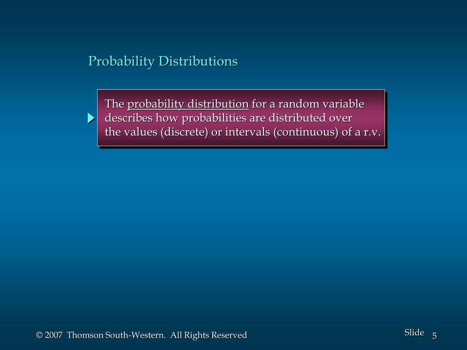
The probability distribution for a random variabledescribes how probabilities are distributed overthe values (discrete) or intervals (continuous) of a r.v.
Probability Distributions
6Slide© 2007 Thomson South-Western. All Rights Reserved
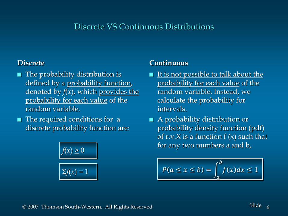
Discrete VS Continuous Distributions
Discrete
The probability distribution is defined by a probability function, denoted by f(x), which provides the probability for each value of the random variable.
The required conditions for a discrete probability function are:
Continuous
It is not possible to talk about the probability for each value of the random variable. Instead, we calculate the probability for intervals.
A probability distribution or probability density function (pdf) of r.v.X is a function f (x) such that for any two numbers a and b,
f(x) > 0
f(x) = 1 𝑃 𝑎 ≤ 𝑥 ≤ 𝑏 = 𝑎
𝑏
𝑓 𝑥 𝑑𝑥 ≤ 1
7Slide© 2007 Thomson South-Western. All Rights Reserved
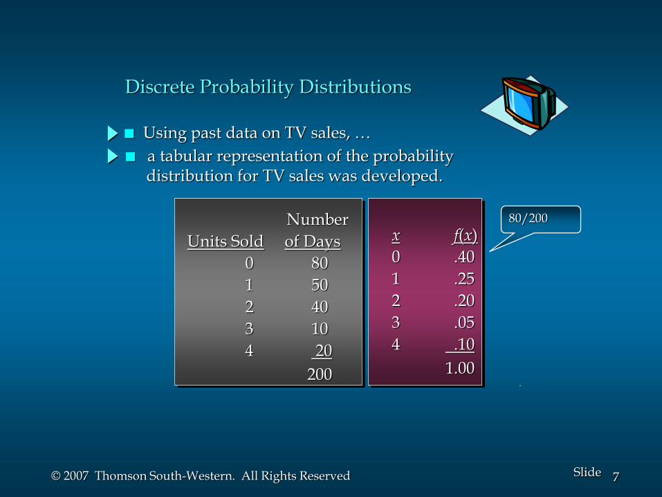
a tabular representation of the probabilitydistribution for TV sales was developed.
Using past data on TV sales, …
Number
Units Sold of Days
0 80
1 50
2 40
3 10
4 20
200
x f(x)
0 .40
1 .25
2 .20
3 .05
4 .10
1.00
80/200
Discrete Probability Distributions

8Slide© 2007 Thomson South-Western. All Rights Reserved
Continuous Probability Distributions
The probability of the random variable assuming a value within some given interval from x1 to x2 is defined to be the area under the graph of the probability density function between x1 and x2.
x
f (x)Normal
x1 x2
𝑃 𝑥1 ≤ 𝑥 ≤ 𝑥2 = 𝑃 𝑥1 < 𝑥 ≤ 𝑥2= 𝑃 𝑥1 ≤ 𝑥 < 𝑥2= 𝑃(𝑥1 < 𝑥 < 𝑥2)
9Slide© 2007 Thomson South-Western. All Rights Reserved
The probability distribution of a random variable, if known, can be used to calculate the mean, variance, skewness, kurtosis and all other descriptive statistics of the random variable.
Using the probability distribution – f(x)

10Slide© 2007 Thomson South-Western. All Rights Reserved
Expected Value, Variance, Std. Deviation
Discrete
Expected value, or mean:
Variance
Standard deviation
Continuous
2 = E (x - )2 = (x - )2f(x)
=E(x) = xf(x) 𝐸 𝑥 = −∞
+∞
𝑥𝑓 𝑥 𝑑𝑥
𝜎2 = −∞
+∞
𝑥 − 𝜇 2𝑓 𝑥 𝑑𝑥
Expected value, or mean:
Variance
Standard deviation
𝜎 = 𝜎2 𝜎 = 𝜎2
11Slide© 2007 Thomson South-Western. All Rights Reserved
CUMULATIVE DISTRIBUTIONS FUNCTIONS
More on distributions…

12Slide© 2007 Thomson South-Western. All Rights Reserved
Definition of CDF
The cumulative distribution function, F(x) for a random variable X is defined for every number x as the probability that the r.v. will take any value up to x, i.e.
𝐹 𝑥 = 𝑃(𝑋 ≤ 𝑥)
e.g. 𝐹 3 = 𝑃 𝑋 ≤ 3𝐹 −1 = 𝑃(𝑋 ≤ −1)
and so on…
13Slide© 2007 Thomson South-Western. All Rights Reserved
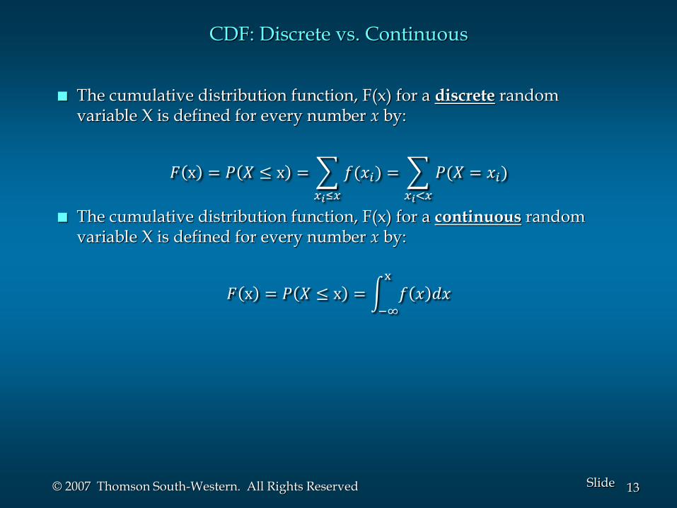
CDF: Discrete vs. Continuous
The cumulative distribution function, F(x) for a discrete random variable X is defined for every number x by:
𝐹 x = 𝑃 𝑋 ≤ x =
𝑥𝑖≤𝑥
𝑓(𝑥𝑖) =
𝑥𝑖<𝑥
𝑃(𝑋 = 𝑥𝑖)
The cumulative distribution function, F(x) for a continuous random variable X is defined for every number x by:
𝐹 x = 𝑃 𝑋 ≤ x = −∞
x
𝑓 𝑥 𝑑𝑥

14Slide© 2007 Thomson South-Western. All Rights Reserved
CDF Properties
A CDF is never decreasing (i.e. as x increases, the CDF will never decrease)
A CDF is always between 0 and 1
For a continuous random variable, the CDF, F(x), can also be used as follows:
𝑃 𝑥 ≥ 𝑎 = 1 − P x ≤ 𝑎 = 1 − 𝐹 𝑎
𝑃 𝑎 ≤ 𝑥 ≤ 𝑏 = 𝐹 𝑏 − 𝐹(𝑎)
How the above relations change if the distribution is discrete?

15Slide© 2007 Thomson South-Western. All Rights Reserved
THE UNIFORM AND NORMAL DISTRIBUTIONS
Important continuous distributions…

16Slide© 2007 Thomson South-Western. All Rights Reserved
Uniform Probability Distribution
where: a = smallest value the variable can assume
b = largest value the variable can assume
f (x) = 1/(b – a) for a < x < b= 0 elsewhere
A random variable is uniformly distributedwhenever the probability is proportional to the interval’s length.
The uniform probability density function is:

17Slide© 2007 Thomson South-Western. All Rights Reserved
Var(x) = (b - a)2/12
E(x) = (a + b)/2
Uniform Probability Distribution
Expected Value of x
Variance of x

18Slide© 2007 Thomson South-Western. All Rights Reserved
Uniform Probability Distribution
Example: Slater's Buffet
Slater customers are charged
for the amount of salad they take.
Sampling suggests that the
amount of salad taken is
uniformly distributed
between 5 ounces and 15 ounces.
19Slide© 2007 Thomson South-Western. All Rights Reserved
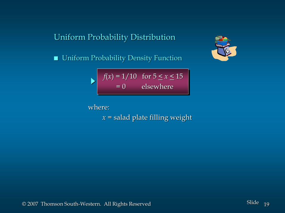
Uniform Probability Density Function
f(x) = 1/10 for 5 < x < 15
= 0 elsewhere
where:
x = salad plate filling weight
Uniform Probability Distribution

20Slide© 2007 Thomson South-Western. All Rights Reserved
Expected Value of x
Variance of x
E(x) = (a + b)/2
= (5 + 15)/2
= 10
Var(x) = (b - a)2/12
= (15 – 5)2/12
= 8.33
Uniform Probability Distribution
21Slide© 2007 Thomson South-Western. All Rights Reserved
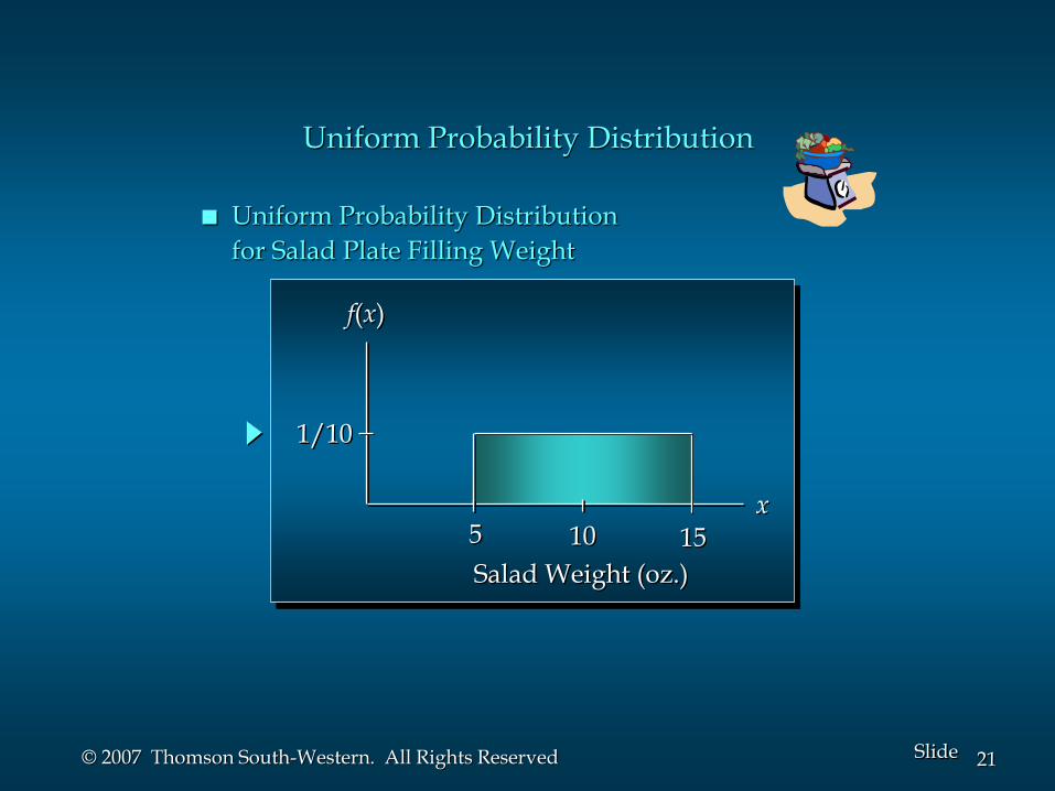
Uniform Probability Distribution
Uniform Probability Distribution
for Salad Plate Filling Weight
f(x)
x5 10 15
1/10
Salad Weight (oz.)
22Slide© 2007 Thomson South-Western. All Rights Reserved
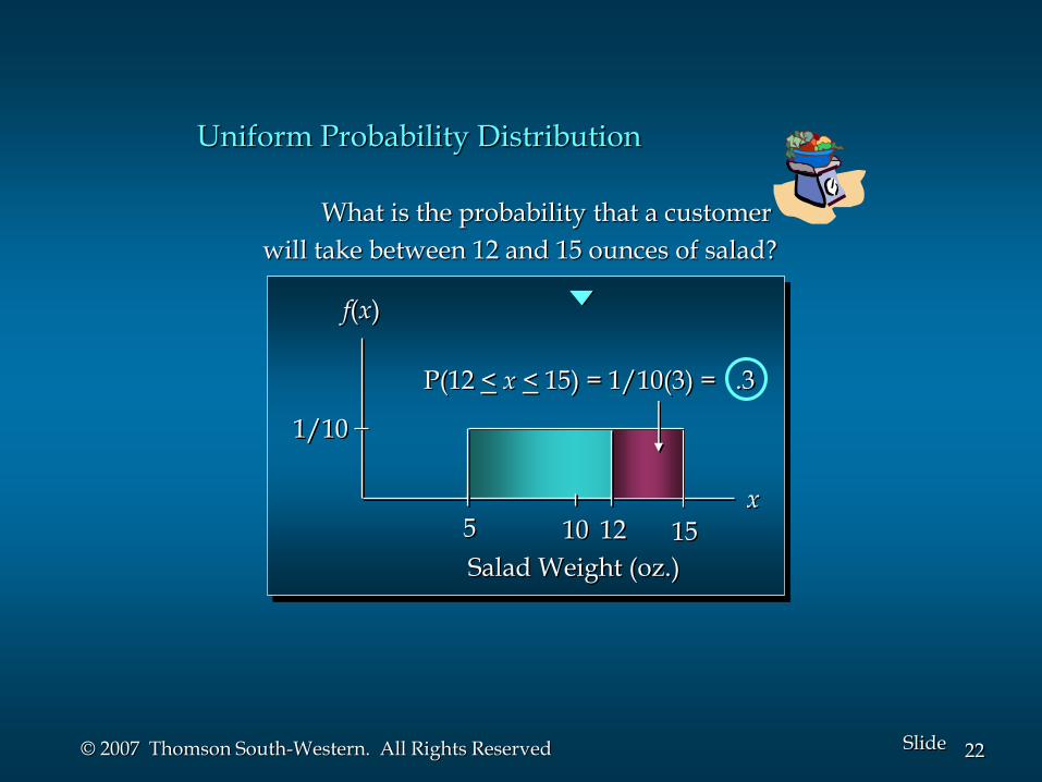
f(x)
x5 10 15
1/10
Salad Weight (oz.)
P(12 < x < 15) = 1/10(3) = .3
What is the probability that a customer
will take between 12 and 15 ounces of salad?
12
Uniform Probability Distribution

23Slide© 2007 Thomson South-Western. All Rights Reserved
Normal Probability Distribution
The normal probability distribution is the most important distribution for describing a continuous random variable.
It is widely used in statistical inference.

24Slide© 2007 Thomson South-Western. All Rights Reserved
Heightsof people
Normal Probability Distribution
It has been used in a wide variety of applications:
Scientificmeasurements

25Slide© 2007 Thomson South-Western. All Rights Reserved
Amounts
of rainfall
Normal Probability Distribution
It has been used in a wide variety of applications:
Testscores

26Slide© 2007 Thomson South-Western. All Rights Reserved
Normal Probability Distribution
Normal Probability Density Function
2 2( ) /21( )
2
xf x e
= mean
= standard deviation
= 3.14159
e = 2.71828
where:

27Slide© 2007 Thomson South-Western. All Rights Reserved
The distribution is symmetric; its skewnessmeasure is zero.
Normal Probability Distribution
Characteristics
x

28Slide© 2007 Thomson South-Western. All Rights Reserved
The entire family of normal probability
distributions is defined by its mean and itsstandard deviation .
Normal Probability Distribution
Characteristics
Standard Deviation
Mean
x

29Slide© 2007 Thomson South-Western. All Rights Reserved
The highest point on the normal curve is at themean, which is also the median and mode.
Normal Probability Distribution
Characteristics
x

30Slide© 2007 Thomson South-Western. All Rights Reserved
Normal Probability Distribution
Characteristics
-10 0 20
The mean can be any numerical value: negative,zero, or positive.
x
31Slide© 2007 Thomson South-Western. All Rights Reserved
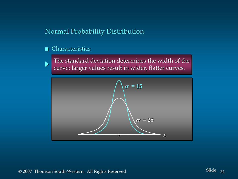
Normal Probability Distribution
Characteristics
= 15
= 25
The standard deviation determines the width of thecurve: larger values result in wider, flatter curves.
x

32Slide© 2007 Thomson South-Western. All Rights Reserved
Probabilities for the normal random variable aregiven by areas under the curve. The total areaunder the curve is 1 (.5 to the left of the mean and.5 to the right).
Normal Probability Distribution
Characteristics
.5 .5
x

33Slide© 2007 Thomson South-Western. All Rights Reserved
Normal Probability Distribution
Characteristics
of values of a normal random variable
are within of its mean.
68.26%
+/- 1 standard deviation
of values of a normal random variable
are within of its mean.
95.44%
+/- 2 standard deviations
of values of a normal random variable
are within of its mean.
99.72%
+/- 3 standard deviations

34Slide© 2007 Thomson South-Western. All Rights Reserved
Normal Probability Distribution
Characteristics
x – 3 – 1
– 2
+ 1
+ 2
+ 3
68.26%
95.44%
99.72%

35Slide© 2007 Thomson South-Western. All Rights Reserved
Standard Normal Probability Distribution
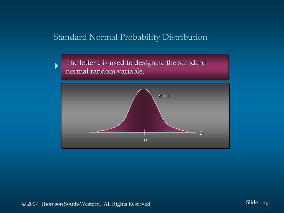
A random variable having a normal distributionwith a mean of 0 and a standard deviation of 1 issaid to have a standard normal probabilitydistribution.
36Slide© 2007 Thomson South-Western. All Rights Reserved
1
0
z
The letter z is used to designate the standardnormal random variable.
Standard Normal Probability Distribution

37Slide© 2007 Thomson South-Western. All Rights Reserved
Converting to the Standard Normal Distribution
Standard Normal Probability Distribution
zx
We can think of z as a measure of the number ofstandard deviations x is from .

38Slide© 2007 Thomson South-Western. All Rights Reserved
Standard Normal Probability Distribution
Example: Pep Zone
Pep Zone sells auto parts and supplies including
a popular multi-grade motor oil. When the
stock of this oil drops to 20 gallons, a
replenishment order is placed.PepZone
5w-20Motor Oil

39Slide© 2007 Thomson South-Western. All Rights Reserved
The store manager is concerned that sales are being
lost due to stockouts while waiting for an order.
It has been determined that demand during
replenishment lead-time is normally
distributed with a mean of 15 gallons and
a standard deviation of 6 gallons.
The manager would like to know the
probability of a stockout, P(x > 20).
Standard Normal Probability Distribution
PepZone
5w-20Motor Oil
Example: Pep Zone

40Slide© 2007 Thomson South-Western. All Rights Reserved
z = (x - )/
= (20 - 15)/6
= .83
Solving for the Stockout Probability
Step 1: Convert x to the standard normal distribution.
PepZone5w-20Motor Oil
Step 2: Find the area under the standard normalcurve to the left of z = .83.
see next slide
Standard Normal Probability Distribution

41Slide© 2007 Thomson South-Western. All Rights Reserved
Cumulative Probability Table for
the Standard Normal Distribution
z .00 .01 .02 .03 .04 .05 .06 .07 .08 .09
. . . . . . . . . . .
.5 .6915 .6950 .6985 .7019 .7054 .7088 .7123 .7157 .7190 .7224
.6 .7257 .7291 .7324 .7357 .7389 .7422 .7454 .7486 .7517 .7549
.7 .7580 .7611 .7642 .7673 .7704 .7734 .7764 .7794 .7823 .7852
.8 .7881 .7910 .7939 .7967 .7995 .8023 .8051 .8078 .8106 .8133
.9 .8159 .8186 .8212 .8238 .8264 .8289 .8315 .8340 .8365 .8389
. . . . . . . . . . .
PepZone5w-20Motor Oil
P(z < .83)
Standard Normal Probability Distribution
42Slide© 2007 Thomson South-Western. All Rights Reserved
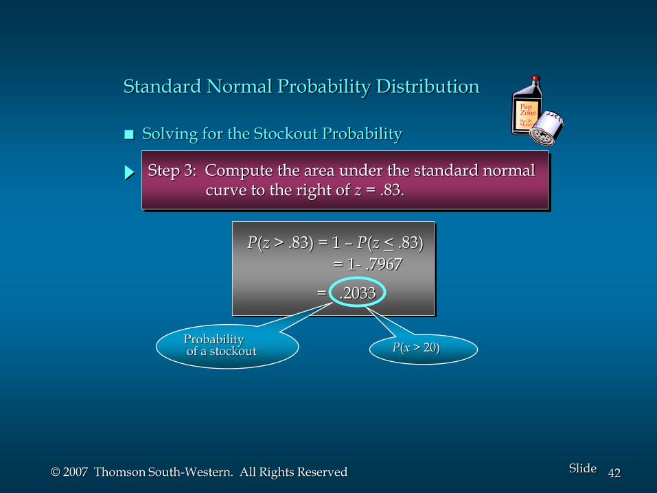
P(z > .83) = 1 – P(z < .83)
= 1- .7967
= .2033
Solving for the Stockout Probability
Step 3: Compute the area under the standard normalcurve to the right of z = .83.
PepZone5w-20Motor Oil
Probabilityof a stockout P(x > 20)
Standard Normal Probability Distribution

43Slide© 2007 Thomson South-Western. All Rights Reserved
Solving for the Stockout Probability
0 .83
Area = .7967Area = 1 - .7967
= .2033
z
PepZone5w-20Motor Oil
Standard Normal Probability Distribution

44Slide© 2007 Thomson South-Western. All Rights Reserved
If the manager of Pep Zone wants the probability of a stockout to be no more than .05, what should the reorder point be?
PepZone5w-20Motor Oil
Inverse of the Standard Normal Probability Distribution

45Slide© 2007 Thomson South-Western. All Rights Reserved
Solving for the Reorder Point
PepZone5w-20Motor Oil
0
Area = .9500
Area = .0500
zz.05
Standard Normal Probability Distribution

46Slide© 2007 Thomson South-Western. All Rights Reserved
Solving for the Reorder Point
PepZone5w-20Motor Oil
Step 1: Find the z-value that cuts off an area of .05in the right tail of the standard normaldistribution.
z .00 .01 .02 .03 .04 .05 .06 .07 .08 .09
. . . . . . . . . . .
1.5 .9332 .9345 .9357 .9370 .9382 .9394 .9406 .9418 .9429 .9441
1.6 .9452 .9463 .9474 .9484 .9495 .9505 .9515 .9525 .9535 .9545
1.7 .9554 .9564 .9573 .9582 .9591 .9599 .9608 .9616 .9625 .9633
1.8 .9641 .9649 .9656 .9664 .9671 .9678 .9686 .9693 .9699 .9706
1.9 .9713 .9719 .9726 .9732 .9738 .9744 .9750 .9756 .9761 .9767
. . . . . . . . . . .
We look up the complement of the tail area (1 - .05 = .95)
Standard Normal Probability Distribution

47Slide© 2007 Thomson South-Western. All Rights Reserved
Solving for the Reorder Point
PepZone5w-20Motor Oil
Step 2: Convert z.05 to the corresponding value of x.
x = + z.05
= 15 + 1.645(6)
= 24.87 or 25
A reorder point of 25 gallons will place the probabilityof a stockout during leadtime at (slightly less than) .05.
Standard Normal Probability Distribution

48Slide© 2007 Thomson South-Western. All Rights Reserved
Solving for the Reorder Point
PepZone5w-20Motor Oil
By raising the reorder point from 20 gallons to 25 gallons on hand, the probability of a stockoutdecreases from about .20 to .05.This is a significant decrease in the chance that PepZone will be out of stock and unable to meet acustomer’s desire to make a purchase.
Standard Normal Probability Distribution

49Slide© 2007 Thomson South-Western. All Rights Reserved
Other Common Continuous distributions
Student’s t
• Hypothesis testing, confidence intervals, prediction intervals, modelling errors that have “heavier” tails than normal.
F
• ANOVA (Analysis of Variance), multiple hypothesis testing
Chi-square
• Hypothesis testing and ANOVA (variance estimation)
Logistic distributions
• Logistic regression
Lognormal Distribution
• Describing prices (economics) and stock market prices
Exponential Probability Distribution
• Describing the time it takes to complete a task
50Slide© 2007 Thomson South-Western. All Rights Reserved
End of distributions review (Chapter 5 & 6)