Review ofMarkov Chain Theory - Wayne State Universityhzhang/courses/7290/Lectures/14 - Review...

Review of Markov Chain Theory

Queuing Analysis:

Hongwei Zhang

http://www.cs.wayne.edu/~hzhang

Acknowledgement: this lecture is partially based on the slides of Dr. Yannis A. Korilis.

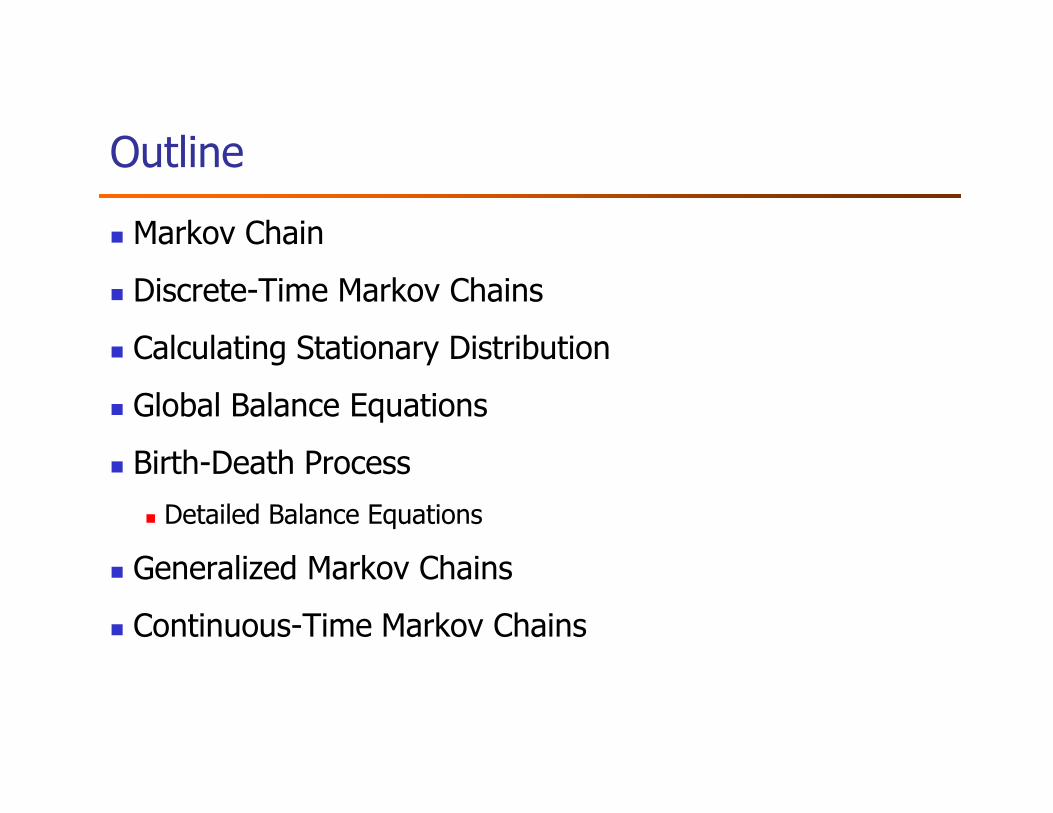
Outline

� Markov Chain

� Discrete-Time Markov Chains

� Calculating Stationary Distribution

� Global Balance Equations� Global Balance Equations

� Birth-Death Process

� Detailed Balance Equations

� Generalized Markov Chains

� Continuous-Time Markov Chains

Markov Chain?

� Stochastic process that takes values in a countable set

� Example: {0,1,2,…,m}, or {0,1,2,…}

� Elements represent possible “states”

� Chain transits from state to state� Chain transits from state to state

� Memoryless (Markov) Property: Given the present state,

future transitions of the chain are independent of past

history

� Markov Chains: discrete- or continuous- time

Outline

� Markov Chain








Discrete-Time Markov Chain

� Discrete-time stochastic process {Xn: n = 0,1,2,…}

� Takes values in {0,1,2,…}

� Memoryless property:

1 1 1 0 0 1{ | , ,..., } { | }n n n n n nP X j X i X i X i P X j X i+ − − += = = = = = =

� Transition probabilities Pij

� Transition probability matrix P=[Pij]

1 1 1 0 0 1

1

{ | , ,..., } { | }

{ | }

n n n n n n

ij n n

P X j X i X i X i P X j X i

P P X j X i

+ − − +

+

= = = = = = =

= = =

0

0, 1ij ij

j

P P∞

=

≥ =∑

� n step transition probabilities

� How to calculate?

Chapman-Kolmogorov Equations

{ | }, , 0, , 0n

ij n m mP P X j X i n m i j+= = = ≥ ≥

� Chapman-Kolmogorov equations

� is element (i, j) in matrix Pn

� Recursive computation of state probabilities

n

ijP

0

, , 0, , 0n m n m

ij ik kj

k

P P P n m i j∞

+

=

= ≥ ≥∑

State Probabilities – Stationary Distribution

� State probabilities (time-dependent)

� In matrix form:

1

1 1

0 0

{ } { } { | } π πn n

n n n n j i ij

i i

P X j P X i P X j X i P∞ ∞

−

− −= =

= = = = = ⇒ =∑ ∑

0 1π { }, π (π ,π ,...)n n n n

j nP X j= = =

� In matrix form:

� If time-dependent distribution converges to a limit

π is called the stationary distribution (or steady state

distribution)

� existence depends on the structure of Markov chain

1 2 2 0π π π ... π

n n n nP P P

− −= = = =

π limπn

n→∞= π πP=

Aperiodic:

� State i is periodic:

� Aperiodic Markov chain: none of

the states is periodic

Classification of Markov Chains

Irreducible:

� States i and j communicate:

� Irreducible Markov chain: all

states communicate

, : 0, 0n m

ij jin m P P∃ > > 1: 0n

iid P n dα∃ > > ⇒ =

the states is periodicstates communicate

0

3 4

21

0

3 4

21

Limit Theorems

Theorem 1: Irreducible aperiodic Markov chain

� For every state j, the following limit

0π lim { | }, 0,1,2,...j nn

P X j X i i→∞

= = = =

exists and is independent of initial state i

� Nj(k): number of visits to state j up to time k

=>πj: frequency the process visits state j

0

( )π lim 1

j

jk

N kP X i

k→∞

= = =

Existence of Stationary Distribution

Theorem 2: Irreducible aperiodic Markov chain. There

are two possibilities for scalars:

1. πj = 0, for all states j No stationary distribution

0π lim { | } lim n

j n ijn n

P X j X i P→∞ →∞

= = = =

1. πj = 0, for all states j No stationary distribution

2. πj > 0, for all states j π is the unique stationary

distribution

Remark: If the number of states is finite, case 2 is the only

possibility

Ergodic Markov Chains

� A state j is positive recurrent if the process returns to state j “infinitely

often”

� Formal definition:

� Fij(n) (n≥1): the probability, given X0 = i, that state j occurs at some time

between 1 and n inclusivebetween 1 and n inclusive

� Tij: the first passage time from i to j

� A state j is recurrent (or persistent) if Fjj(∞) = 1, and transient otherwise

� A state j is positive recurrent (or non-null persistent) if Fjj(∞) = 1 and E(Tjj) < ∞

� A state j is null recurrent (or null persistent) if Fjj(∞) = 1 but E(Tjj) = ∞

� Note: “positive recurrent => irreducible” always hold, but “irreducible =>

positive recurrent” is guaranteed to hold only for finite MC

Ergodic MC (contd.)

� Example: a MC with countably infinite state space

0 1 2 3 4 5 • • •

p

q = 1-p

p p p p p

qqqqq

q

� All states are positive recurrent if p < ½, null recurrent if p = ½, and

transient if p > ½

� A state is ergodic if it is aperiodic and positive recurrent

� A MC is ergodic if every state is ergodic

� Ergodic chains have a unique stationary distribution

πj = 1/E(Tjj), j = 0, 1, 2, …

� Note: Ergodicity ⇒ Time Averages = Stochastic Averages

Outline

� Markov Chain








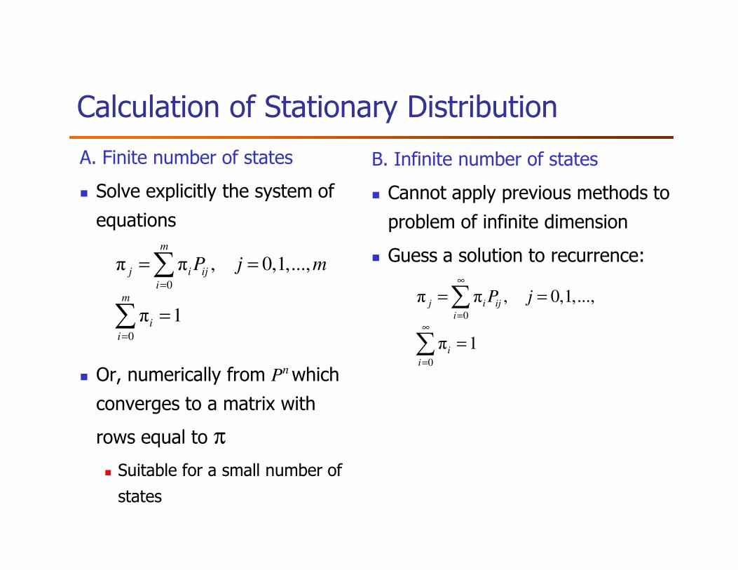
Calculation of Stationary Distribution

A. Finite number of states

� Solve explicitly the system of

equations

B. Infinite number of states

� Cannot apply previous methods to

problem of infinite dimension

� Guess a solution to recurrence:

0

π π , 0,1,...,m

j i ij

i

P j m=

= =∑∞

= =∑

� Or, numerically from Pn which

converges to a matrix with

rows equal to π

� Suitable for a small number of

states

0

0

π 1

i

m

i

i

=

=

=∑ 0

0

π π , 0,1,...,

π 1

j i ij

i

i

i

P j∞

=∞

=

= =

=

∑

∑

Example: Finite Markov Chain

� Markov chain formulation

� i is the number of umbrellas

available at her current location

� Absent-minded professor uses

two umbrellas when commuting

between home and office.

� If it rains and an umbrella is

available at her location, she 0 2 1 1 p−

1 p

� Transition matrix

available at her location, she

takes it. If it does not rain, she

always forgets to take an

umbrella.

� Let p be the probability of rain

each time she commutes.

Q: What is the probability that

she gets wet on any given day?

0 2 1 1 p−

p1 p−

0 0 1

0 1

1 0

P p p

p p

= −

−


0 2 1 1 p−

p1 p−

1 p0 0 1

0 1

1 0

P p p

p p

= −

−

π (1 )πp= −

2 0

0 2

1 1 2

0 1 2

1 2

1

0

π π π

π (1 )π

π π π (1 )π π 1 1 1π , π , π

π 1 3 3 3

π π π 1

i i

p

P p p p

pp p p

= −= = − + −

⇔ ⇔ = = = = − − −

+ + =

= +

∑

0

1{gets wet} π

3

pP p p

p

−= =

−


� Taking p = 0.1:

0 0 1

0 0.9 0.1

0.9 0.1 0

P

=

( )1 1 1

π , , 0.310, 0.345, 0.3453 3 3

p

p p p

−= = − − −

� Numerically determine limit of Pn

� Effectiveness depends on structure of P

0.9 0.1 0

0.310 0.345 0.345

lim 0.310 0.345 0.345 ( 150)

0.310 0.345 0.345

n

nP n

→∞

= ≈

Outline

� Markov Chain








Global Balance Equations

� Global Balance Equations (GBE)

� is the frequency of transitions from j to i

0 0

π π π π , 0j ji i ij j ji i ij

i i i j i j

P P P P j∞ ∞

= = ≠ ≠

= ⇔ = ≥∑ ∑ ∑ ∑

πj jiP

Frequency of Frequency of

� Intuition: 1) j visited infinitely often; 2) for each transition out of j there must be a subsequent transition into j with probability 1

Frequency of Frequency of

transitions out of transitions into j j

=

Global Balance Equations (contd.)

� Alternative Form of GBE

� If a probability distribution satisfies the GBE, then it is

{ }π π , 0,1,2,...j ji i ij

j S i S i S j S

P P S∈ ∉ ∉ ∈

= ⊆∑ ∑ ∑ ∑

the unique stationary distribution of the Markov chain

� Finding the stationary distribution:

� Guess distribution from properties of the system

� Verify that it satisfies the GBE

☺Special structure of the Markov chain simplifies task

Global Balance Equations – Proof

0 0

0 0

π π and 1

π π π π

j i ij ji

i i

j ji i ij j ji i ij

i i i j i j

P P

P P P P

∞ ∞

= =∞ ∞

= = ≠ ≠

= = ⇒

= ⇔ =

∑ ∑

∑ ∑ ∑ ∑

First form:

0 0 0 0

π π π π

π π π

π π

j ji i ij j ji i ij

i i j S i j S i

j ji ji i ij i ij

j S i S i S j S i S i S

j ji i ij

j S i S i S j S

P P P P

P P P P

P P

∞ ∞ ∞ ∞

= = ∈ = ∈ =

∈ ∈ ∉ ∈ ∈ ∉

∈ ∉ ∉ ∈

= ⇒ = ⇒

+ = + ⇒

=

∑ ∑ ∑ ∑ ∑∑

∑ ∑ ∑ ∑ ∑ ∑

∑ ∑ ∑ ∑

Second form:

Outline

� Markov Chain








Birth-Death Process

� One-dimensional Markov chain with transitions only

0 1 n+1n2

, 1n nP +

1,n nP +,n nP, 1n nP −

1,n nP −01P

10P00P

S Sc

� One-dimensional Markov chain with transitions only

between neighboring states: Pij=0, if |i-j|>1

� Detailed Balance Equations (DBE)

� Proof: GBE with S ={0,1,…,n} give:

, 1 1 1,π π 0,1,...n n n n n nP P n+ + += =

, 1 1 1,

0 1 0 1

π π π π

n n

j ji i ij n n n n n n

j i n j i n

P P P P∞ ∞

+ + += = + = = +

= ⇒ =∑∑ ∑∑

Example: Discrete-Time Queue

� In a time-slot, one packet arrival with probability p or zero

arrivals with probability 1-p

� In a time-slot, the packet in service departs with probability

q or stays with probability 1-qq or stays with probability 1-q

� Independent arrivals and service times

� State: number of packets in system

0 1 n+1n2

(1 )p−

p (1 )p q−

(1 )(1 )p q pq− − +

(1 )q p− (1 )q p−

p (1 )p q−

(1 )(1 )p q pq− − +(1 )q p−

Example: Discrete-Time Queue (contd.)

0 1 n+1n2

(1 )p−

p (1 )p q−

(1 )(1 )p q pq− − +

(1 )q p− (1 )q p−

(1 )p q−

(1 )(1 )p q pq− − +(1 )q p−

(1 )p q−

0 1 1 0

/π π (1 ) π π

1

p qp q p

p= − ⇒ =

−

1 1

(1 )π (1 ) π (1 ) π π , 1

(1 )n n n n

p qp q q p n

q p+ +

−− = − ⇒ = ≥

−

0 1 1 0π π (1 ) π π1

p q pp

= − ⇒ =−

(1 )Define: / ,

(1 )

p qp q

q pρ α

−≡ ≡

−

1 0 1

0

1

π 1 π π , 1

1π π , 1

n

n

n n

p np

n

ρπ ρ

α

α

−

+

=

− ⇒ = ≥− = ≥

Example: Discrete-Time Queue (contd.)

� Having determined the distribution as a function of π0

How to calculate the normalization constant π0?

� Probability conservation law:

1

0π π , 1

1

n

nn

p

ρα −= ≥

−

1 1− −

� Noting that

1 1

1

00 1

1π 1 π 1 1

1 (1 ) (1 )

n

nn np p

ρ ρα

α

− −∞ ∞ −

= =

= ⇒ = + = + − − −

∑ ∑

( )( ) ( ) ρα −=−

=−

−−−−=−− 1

)1(

)1()1(111

q

pq

pq

qppqpp

0

1

π 1

π (1 ) , 1n

n n

ρ

ρ α α −

= −

= − ≥

Detailed Balance Equations

� General case:

� Need NOT hold for every Markov chain

If hold, it implies the GBE; greatly simplify the calculation of stationary

π π , 0,1,...j ji i ijP P i j= =

� If hold, it implies the GBE; greatly simplify the calculation of stationary

distribution

Methodology:

� Assume DBE hold – have to guess their form

� Solve the system defined by DBE and Σiπi = 1

� If system is inconsistent, then DBE does not hold

� If system has a solution {πi: i=0,1,…}, then it is the unique stationary distribution

Outline

� Markov Chain








Generalized Markov Chains

� Markov chain on a set of states {0,1,…}, that whenever enters state i

� The next state that will be entered is j with probability Pij

� Given that the next state entered will be j, the time it spends at state i until

the transition occurs is a RV with distribution Fij

� {Z(t): t ≥ 0} describing the state of the chain at time t: Generalized

Markov chain, or Semi-Markov process

� Does GMC have the Markov property?

� Future depends on 1) the present state, and 2) the length of time the process has

spent in this state

Generalized Markov Chains (contd.)

� Ti: time process spends at state i, before making a transition – holding

time

� Probability distribution function of Ti

0 0

( ) { } { | next state } ( )i i i ij ij ij

j j

H t P T t P T t j P F t P∞ ∞

= =

= ≤ = ≤ =∑ ∑[ ] ( )E T t dH t

∞

= ∫� Tii: time between successive transitions to i

� Xn is the nth state visited. {Xn: n=0,1,…}

� Is a Markov chain: embedded Markov chain

� Has transition probabilities Pij

� Semi-Markov process irreducible: if its embedded Markov chain is

irreducible

0[ ] ( )

i iE T t dH t

∞

= ∫

Limit Theorems

Theorem 3: given an irreducible semi-Markov process w/ E[Tii] < ∞

� For any state j, the following limit

exists and is independent of the initial state.

lim { ( ) | (0) }, 0,1,2,...j

tp P Z t j Z i i

→∞= = = =

[ ]j

E T=

� Tj(t): time spent at state j up to time t

� pj is equal to the proportion of time spent at state j

[ ]

[ ]

j

j

jj

E Tp

E T=

( )lim (0) 1

j

jt

T tP p Z i

t→∞

= = =

Occupancy Distribution

Theorem 4: given an irreducible semi-Markov process where E[Tii] < ∞,

and the embedded Markov chain is ergodic w/ stationary distribution π

� then, with probability 1, the occupancy distribution of the semi-Markov

process

0 0

π π , 0; π 1j i ij i

i i

P j∞ ∞

= =

= ≥ =∑ ∑

process

� πj: proportion of transitions into state j

� E[Tj]: mean time spent at j

Probability of being at j is proportional to πjE[Tj]

π [ ], 0,1,...

π [ ]

j j

j

i i

i

E Tp j

E T= =∑

Outline

� Markov Chain








Continuous-Time Markov Chains (def.?)

Continuous-time process {X(t): t ≥ 0} taking values in {0,1,2,…}.

Whenever it enters state i

� Time it spends at state i is exponentially distributed with parameter νi

� When it leaves state i, it enters state j with probability Pij, where Σj≠i Pijij j≠i ij

= 1

� Continuous-time Markov chain is a semi-Markov process with

� Exponential holding time => a continuous-time Markov chain has the

Markov property

( ) 1 , , 0,1,...it

ijF t e i jν−= − =

Continuous-Time Markov Chains

� When at state i, the process makes transitions to state j≠i

with rate:

Total rate of transitions out of state i

ij i ijq Pν≡

� Total rate of transitions out of state i

� Average time spent at state i before making a transition:

ij i ij i

j i j i

q Pν ν≠ ≠

= =∑ ∑

[ ] 1/i i

E T ν=

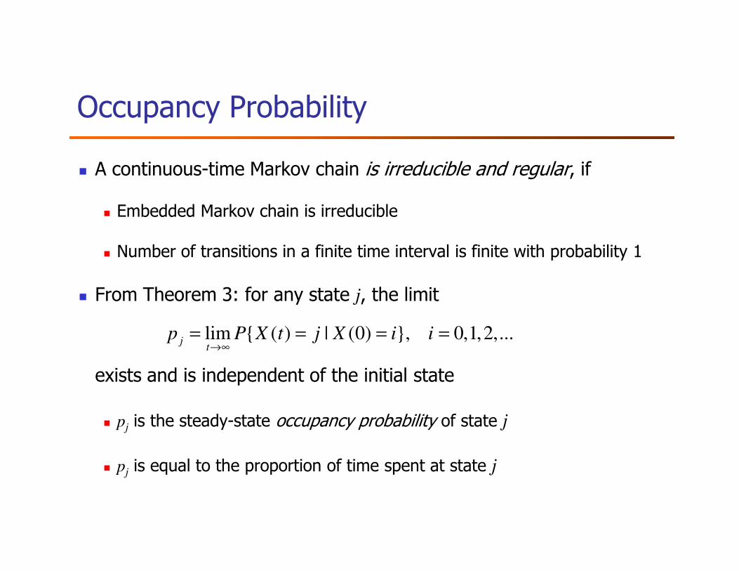
Occupancy Probability

� A continuous-time Markov chain is irreducible and regular, if

� Embedded Markov chain is irreducible

� Number of transitions in a finite time interval is finite with probability 1

From Theorem 3: for any state j, the limit � From Theorem 3: for any state j, the limit

exists and is independent of the initial state

� pj is the steady-state occupancy probability of state j

� pj is equal to the proportion of time spent at state j

lim { ( ) | (0) }, 0,1,2,...j

tp P X t j X i i

→∞= = = =

Global Balance Equations

� Two possibilities for the occupancy probabilities:

� pj= 0, for all j

� pj> 0, for all j, and Σj pj = 1

� Global Balance Equations

, 0,1,...p q p q j= =∑ ∑� Rate of transitions out of j = rate of transitions into j

� If a distribution {pj: j = 0,1,…} satisfies GBE, then it is the unique occupancy

distribution of the Markov chain

� Alternative form of GBE:

, 0,1,...j ji i ij

i j i j

p q p q j≠ ≠

= =∑ ∑

, {0,1,...}j ji i ij

j S i S i S j S

p q p q S∈ ∉ ∉ ∈

= ⊆∑ ∑ ∑ ∑

Detailed Balance Equations


☺ Simplify the calculation of the stationary distribution

Need not hold for every Markov chain

, , 0,1,...j ji i ijp q p q i j= =

� Need not hold for every Markov chain

� Examples: birth-death processes, and reversible Markov

chains

Birth-Death Process

Transitions only between neighboring states

0 1 n+1n2

0λ

1µ

nλ

1nµ +

1λ

2µ

1nλ −

nµ

S Sc

� Transitions only between neighboring states


� Proof: GBE with S ={0,1,…,n} give:

, 1 , 1, , 0, | | 1i i i i i i ijq q q i jλ µ+ −= = = − >

1 1, 0,1,...n n n np p nλ µ + += =

1 1

0 1 0 1

n n

j ji i ij n n n n

j i n j i n

p q p q p pλ µ∞ ∞

+ += = + = = +

= ⇒ =∑∑ ∑∑

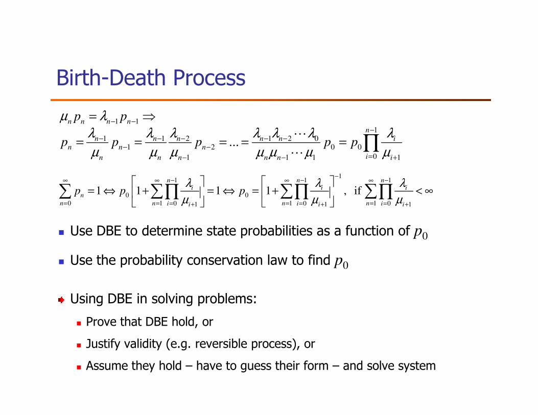
Birth-Death Process

1 11

1 1 2 1 2 01 2 0 0

01 1 1 1

...

n n n nn

n n n n n in n n

in n n n n i

p p

p p p p p

µ λ

λ λ λ λ λ λ λ

µ µ µ µ µ µ µ

− −−

− − − − −− −

=− − +

= ⇒

= = = = = ∏L

L

11 1 1

0 0

0 1 1 10 0 01 1 1

1 1 1 1 , if n n n

i i in

n n n ni i ii i i

p p pλ λ λ

µ µ µ

−− − −∞ ∞ ∞ ∞

= = = == = =+ + +

= ⇔ + = ⇔ = + < ∞

∑ ∑ ∑ ∑∏ ∏ ∏

� Use DBE to determine state probabilities as a function of p0

� Use the probability conservation law to find p0

Using DBE in solving problems:

� Prove that DBE hold, or

� Justify validity (e.g. reversible process), or

� Assume they hold – have to guess their form – and solve system

1 1 1i i i+ + +

M/M/1 Queue

� Arrival process: Poisson with rate λ

� Service times: iid, exponential with parameter µ

� Service times and interarrival times: independent

Single server� Single server

� Infinite waiting room

� N(t): Number of customers in system at time t (state)

0 1 n+1n2

λ

µ

λ

µ

λ

µ

λ

µ

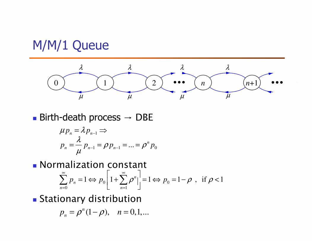
M/M/1 Queue

� Birth-death process → DBE

0 1 n+1n2

λ

µ

λ

µ

λ

µ

λ

µ

� Birth-death process → DBE

� Normalization constant

� Stationary distribution

1

1 1 0...

n n

n

n n n

p p

p p p p

µ λλ

ρ ρµ

−

− −

= ⇒

= = = =

0 0

0 1

1 1 1 1 , if 1n

n

n n

p p pρ ρ ρ∞ ∞

= =

= ⇔ + = ⇔ = − <

∑ ∑

(1 ), 0,1,...n

np nρ ρ= − =

The M/M/1 Queue

� Average number of customers

1

0 0 0

2

(1 ) (1 )

1(1 )

(1 ) 1

n n

n

n n n

N np n n

N

ρ ρ ρ ρ ρ

ρ λρ ρ

ρ ρ µ λ

∞ ∞ ∞−

= = =

= = − = −

⇒ = − = =− − −

∑ ∑ ∑

� Applying Little’s Theorem, we have

� Similarly, the average waiting time and number of customers in

the queue is given by

λµλµ

λ

λλ −=

−==

11NT

ρ

ρλ

λµ

ρ

µ −==

−=−=

1 and

1 2

WNTW Q

Summary

� Markov Chain



Global Balance Equations� Global Balance Equations





Homework #8

� Problem 3.14 of R1

� Hints:

� For a service system, the expected number of customers is finite if the

service rate is greater than the customer arrival rate.

� To solve the problem, think of how to model the system as a Markov

process. You may also find Little's Theorem be of some use in solving the

problem.

� Grading:

� Overall points 100

� 30 points for 3.14(a)

� 70 points for 3.14(b)

Review ofMarkov Chain Theory - Wayne State Universityhzhang/courses/7290/Lectures/14 - Review...

Documents

Transcript of Review ofMarkov Chain Theory - Wayne State Universityhzhang/courses/7290/Lectures/14 - Review...