REVIEW OF RAILGUN MODELING TECHNIQUES: THE …
103
REVIEW OF RAILGUN MODELING TECHNIQUES: THE COMPUTATION OF RAILGUN FORCE AND OTHER KEY FACTORS by NATHAN JAMES ECKERT A thesis submitted to the Faculty of the Graduate School of the University of Colorado in partial fulfillment of the requirement for the degree of Master of Science Department of Aerospace Engineering 2017
Transcript of REVIEW OF RAILGUN MODELING TECHNIQUES: THE …
i
REVIEW OF RAILGUN MODELING TECHNIQUES
THE COMPUTATION OF RAILGUN FORCE AND OTHER KEY FACTORS
by
NATHAN JAMES ECKERT
A thesis submitted to the
Faculty of the Graduate School of the
University of Colorado in partial fulfillment
of the requirement for the degree of
Master of Science
Department of Aerospace Engineering
2017
ii
This thesis entitled
Review of Railgun Modeling Techniques
Computation of Railgun Force and Other Key Factors
written by Nathan James Eckert
has been approved for the Department of Aerospace Engineering
Dr Kurt Maute Chair
Dr Alireza Doostan
Date
The final copy of this thesis has been examined by the signatories and we
find that both the content and the form meet acceptable presentation standards
of scholarly work in the above mentioned discipline
iii
Eckert Nathan James (MS Aerospace Engineering)
Review of Railgun Modeling Techniques Computation of Railgun Force and Other Key Factors
Thesis directed by Professor Kurt Maute
Currently railgun force modeling either uses the simple ldquorailgun force equationrdquo or finite element
methods It is proposed here that a middle ground exists that does not require the solution of partial
differential equations is more readily implemented than finite element methods and is more accurate than
the traditional force equation To develop this method it is necessary to examine the core railgun factors
power supply mechanisms the distribution of current in the rails and in the projectile which slides between
them (called the armature) the magnetic field created by the current flowing through these rails the
inductance gradient (a key factor in simplifying railgun analysis referred to as 119871prime) the resultant Lorentz
force and the heating which accompanies this action Common power supply technologies are investigated
and the shape of their current pulses are modeled The main causes of current concentration are described
and a rudimentary method for computing current distribution in solid rails and a rectangular armature is
shown to have promising accuracy with respect to outside finite element results The magnetic field is
modeled with two methods using the Biot-Savart law and generally good agreement is obtained with
respect to finite element methods (58 error on average) To get this agreement a factor of 2 is added to
the original formulation after seeing a reliable offset with FEM results Three inductance gradient
calculations are assessed and though all agree with FEM results the Kerrisk method and a regression
analysis method developed by Murugan et al (referred to as the LRM here) perform the best Six railgun
force computation methods are investigated including the traditional railgun force equation an equation
produced by Waindok and Piekielny and four methods inspired by the work of Xu et al Overall good
agreement between the models and outside data is found but each modelrsquos accuracy varies significantly
between comparisons Lastly an approximation of the temperature profile in railgun rails originally
presented by McCorkle and Bahder is replicated In total this work describes railgun technology and
moderately complex railgun modeling methods but is inconclusive about the presence of a middle-ground
modeling method
iv
Acknowledgments
This work would not have been possible without the input and support provided to me by
members of the faculty at the University of Colorado at Boulder Though the role of the University as a
whole is significant there are some specific people who deserve thanks
First I would like to thank my advisor Professor Kurt Maute for allowing me to pursue this
research and supporting my efforts along the way The focus of this research is outside the expertise of
much of the department and Dr Maute very well could have told me to examine something more
traditional or chose not to spend his valuable time supporting this work I very much appreciate the
opportunity he has afforded me to develop this thesis
Special thanks goes out to Assistant Professor Robert Marshall and Associate Professor Alireza
Doostan who have also been instrumental in this work by taking their time to assess this work In
particular Dr Marshall has given multiple hours of his time in meetings with me that have undoubtedly
improved the quality of this work
Next I want to thank Professor Hanspeter Schaub who allowed me to share the use of his
ANSYS Maxwell license and improved the quality of the work I was able to perform Dr Schaub could
have easily denied access to ensure his would not have any issues and I appreciate that he trusted I would
work to impose as little as possible on his teamrsquos work
Lastly I want to thank Dr Paul Ibanez my boss and more for being understanding throughout
this research and providing me with a flexible work environment Dr Ibanez also spent a significant
amount of his valuable time meeting with me to discuss the finer points of railgun modeling
v
Contents
Chapter 1 Railgun Background 1
Chapter 2 Power Supply Mechanisms 5
21 Capacitor Banks 9
22 Rotating Machines 10
Chapter 3 Current Distribution 13
31 Clustering Near Small Source (CNSS) 15
32 Clustering Along Short Path (CASP) 16
33 Proximity Effect 16
34 Skin Effect of Alternating Current (SAC) 17
35 Velocity Skin Effect (VSE) 18
36 Current Distribution Approximation (CStSM) 20
37 CStSM Comparison 22
Chapter 4 Magnetic Field 25
41 Comparison to Chen et al 28
42 Comparison to Waindok and Piekielny 34
Chapter 5 Inductance Gradient 40
51 Kerrisk Method 41
52 Huerta Conformal Mapping Method 42
53 Intelligent Estimation Method (IEM) 43
54 119871prime Regression Method (LRM) 44
vi
55 Comparison of 119871prime Methods 45
Chapter 6 Force Computation 50
61 Comparison Case 1 (CC1) Waindok and Piekielny (2016) and ANSYS Maxwell 55
62 Comparison Case 2 (CC2) Chengxue et al (2014) 60
63 Comparison Case 3 (CC3) Jin et al (2015) 62
64 Comparison Case 4 (CC4) Chen et al (Chen 2015) 65
65 Force Comparison Conclusions 70
Chapter 7 Heating 72
Chapter 8 Conclusion 77
References 79
Appendix 85
Appendix A Inductance Gradient Tables 85
Appendix B Inductance Gradient Result Replication 89
vii
List of Tables
Table 1 Railgun Performance vs Conventional Gun Performance 2
Table 2 Railgun parameters used by Lv et al 22
Table 3 Parameters for the Chen et al railgun 28
Table 4 Comparison of ANSYS and FEMM results for the Chen et al case 32
Table 5 Railgun parameters used throughout this paper used by Waindok and Piekielny 34
Table 6 Comparison of MATLAB models vs FEMM for the Waindok and Piekielny railgun 34
Table 7 Kerrisk method coefficients 41
Table 8 LRM regression values 44
Table 9 119871prime analytical method errors vs FEM 47
Table 10 Description of force computation methods 54
Table 11 CC1 Results 56
Table 12 Results produced by Waindok and Piekielny for CC1 55
Table 13 Mesh refinement assessment 56
Table 14 Railgun parameters for comparison case 2 (CC2) 60
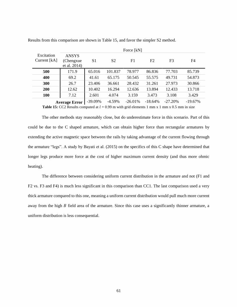
Table 15 CC2 Results 61
Table 16 Railgun parameters for comparison case 3 (CC3) (Jin et al 2015) 62
Table 17 CC3 Results 64
Table 18 Parameters for the Chen et al railgun 65
Table 19 Comparison of the set A experiments from Chen et al to force model results 67
Table 20 Comparison of the set 119861 experiments from Chen et al to force model results 68
Table 21 Overview of force comparison results 70
Table 22 Railgun properties used to replicate the results of McCorkle and Bahder 75
viii
List of Figures
Figure 1 Railgun Concept 1
Figure 2 Pulse forming network schematic 6
Figure 3 Current profiles with I = 250kA 7
Figure 4 Current profiles of railguns that will accelerate projectiles to 3 kms 7
Figure 5 Experimental current profiles 9
Figure 6 The PEGASUS railgun at ISL and part of the capacitor bank that powers it 9
Figure 7 Compulsator current profile 11
Figure 8 Current flow through imperfect electrical contact 15
Figure 9 Railgun concept considering CASP with planes 1 rarr 7 defined for reference 16
Figure 10 Current distribution in rail 18
Figure 11 Current distribution in rail 18
Figure 12 Current concentration due to velocity skin effect 18
Figure 13 Current distribution 23
Figure 14 Current distribution 23
Figure 15 Biot-Savart variable definitions 26
Figure 16 Rear view of the left rail current at 119903prime produces magnetic field at 119903 26
Figure 17 Magnetic field strength in armature for five thickness values 29
Figure 18 Magnetic field strength in armature for five thickness values 29
Figure 19 Magnetic field strength in armature for the Chen et al railgun 30
Figure 20 Orientation of Figure 19 armature magnetic field plots 30
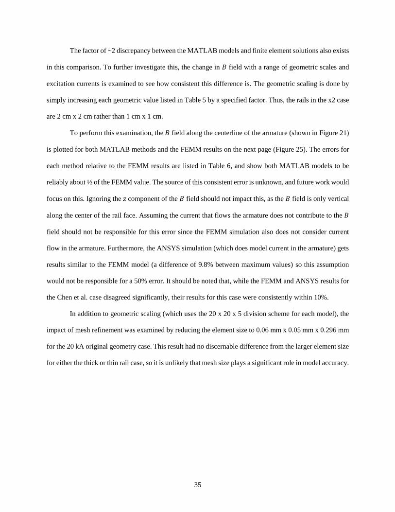
Figure 21 Comparison of MATLAB models vs FEMM 31
Figure 22 FEMM setup 31
Figure 23 FEMM 119861 field results for the Chen et al case 32
Figure 24 ANSYS Maxwell 119861 field results for the Chen et al case 33
ix
Figure 25 Comparison of MATLAB models vs FEMM results for varying scales 36
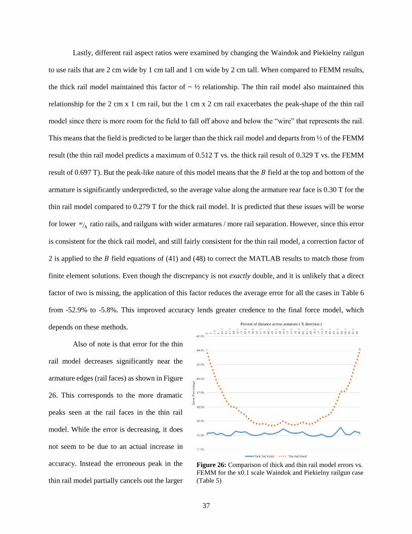
Figure 26 Comparison of thick and thin rail model errors vs FEMM 37
Figure 27 ANSYS Maxwell result for the Waindok and Piekielny railgun 39
Figure 28 Magnetic field strength in armature for the Waindok and Piekielny railgun 39
Figure 29 Dimension description for rectangular rails 40
Figure 30 Dimension description for circular rails 45
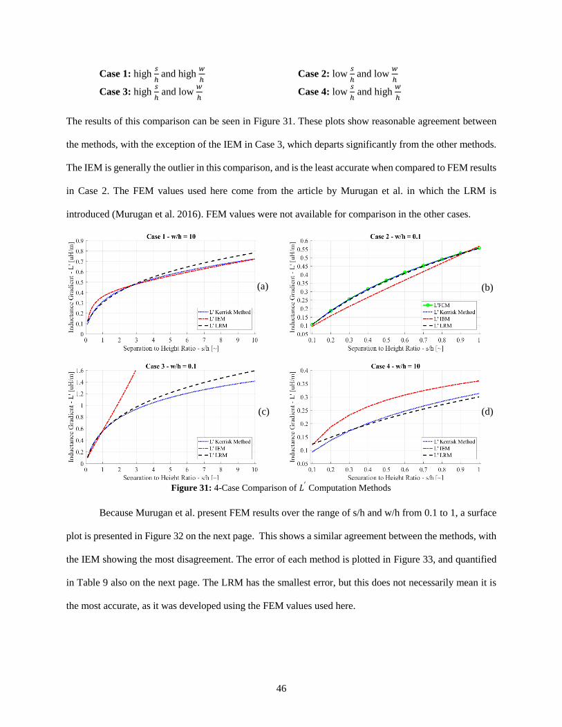
Figure 31 4-Case Comparison of 119871prime Computation Methods 46
Figure 32 Comparison of 119871prime methods to FEM 47
Figure 33 119871prime analytical method error vs FEM 47
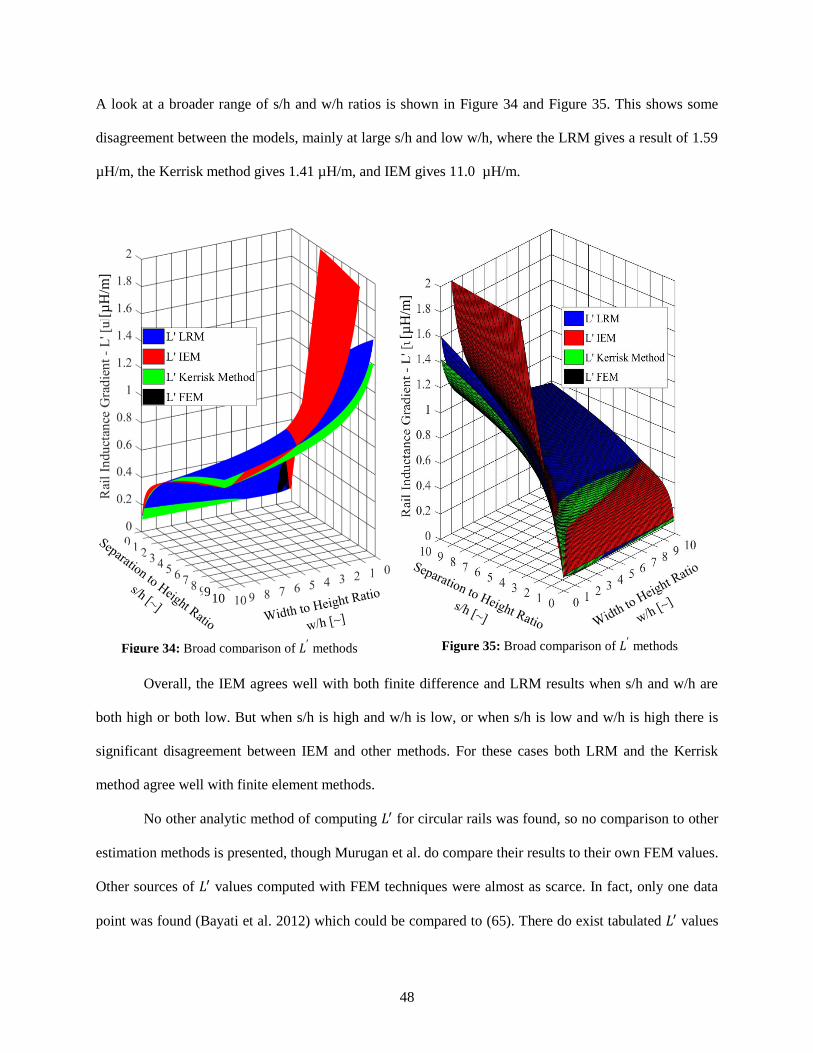
Figure 34 Broad comparison of 119871prime methods 48
Figure 35 Broad comparison of 119871prime methods 48
Figure 36 Magnetic field around rails as computed by ANSYS Maxwell 172 51
Figure 37 Current flow in rails and armature as computed by ANSYS Maxwell 172 52
Figure 38 Special armature used by Chen et al to study melt wear rate 54
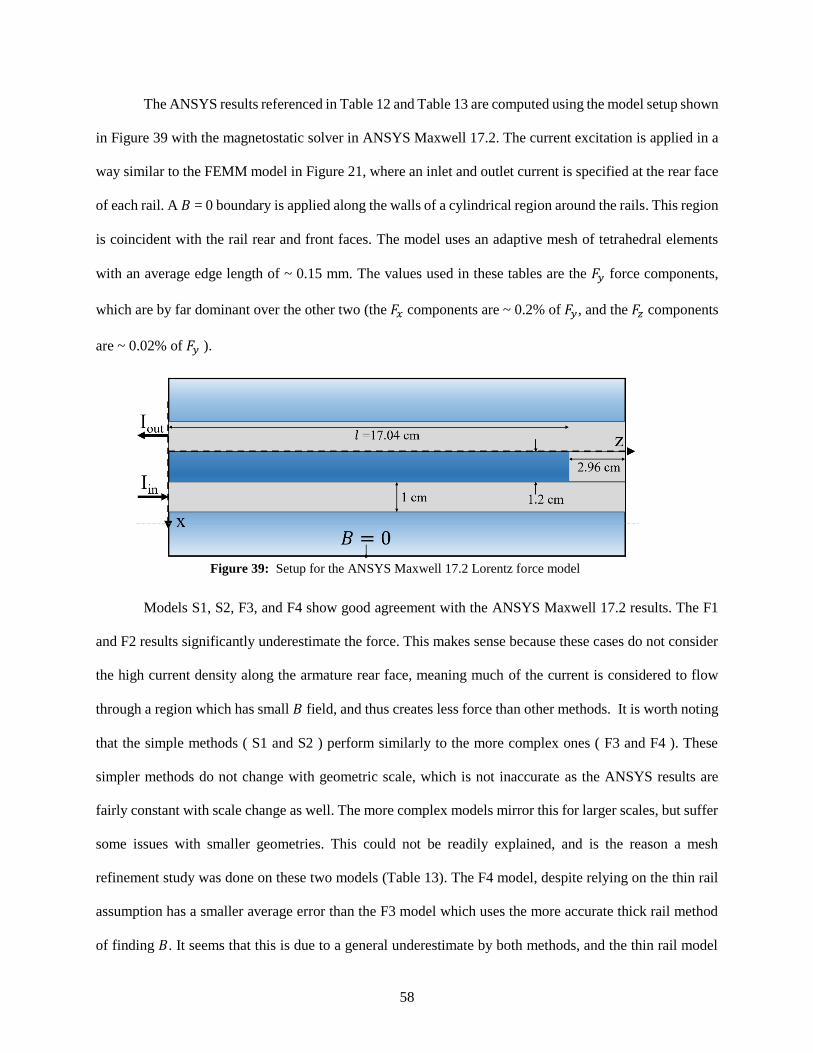
Figure 39 Setup for the ANSYS Maxwell 172 Lorentz force model 58
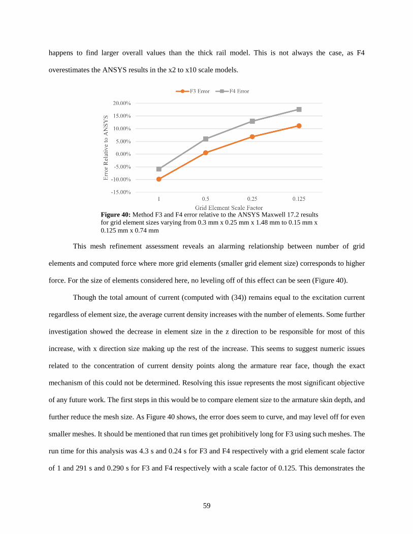
Figure 40 Method F3 and F4 error relative to the ANSYS Maxwell 172 results 59
Figure 41 C armature illustration 60
Figure 42 CC3 current profile 62
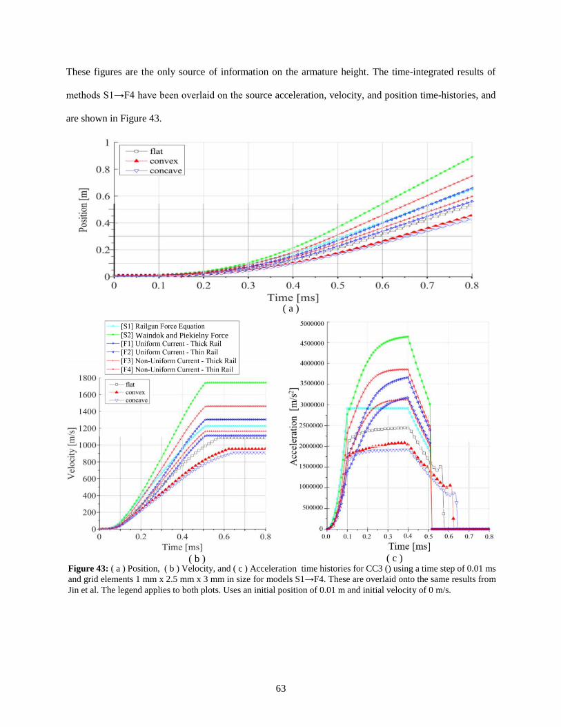
Figure 43 ( a ) Position ( b ) Velocity and ( c ) Acceleration time histories 63
Figure 44 Recorded current profile for ( a ) shot A-2 and ( b ) shot B-3 from Chen et al 66
Figure 45 (a) Position (b) Velocity and (c) Acceleration time histories for CC4 69
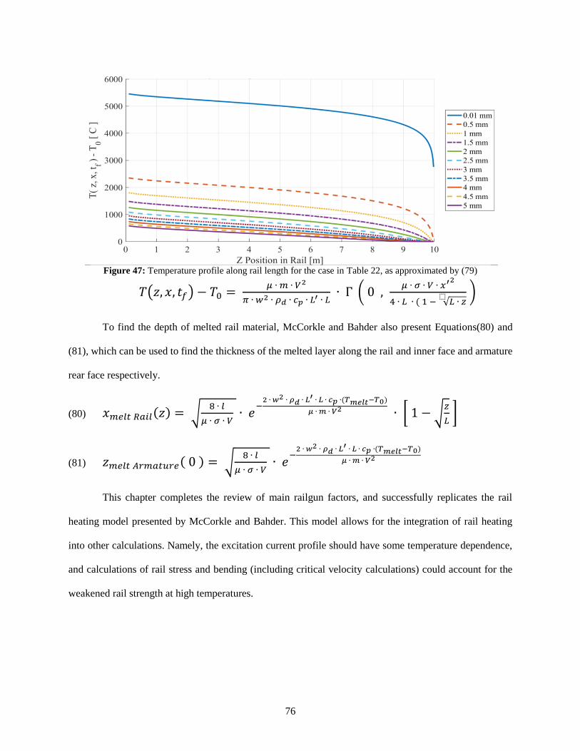
Figure 47 Temperature profile along rail length for the case in Table 22 76
Figure 46 Temperature profile in a railgun rail 75
Figure 49 119871prime and Maximum Current Density 85
Figure 50 119871prime as Simulated by Asghar Keshtkar (2005) 85
x
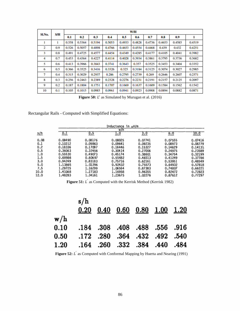
Figure 51 119871prime as Simulated by Murugan et al (2016) 86
Figure 52 119871prime as Computed with the Kerrisk Method (Kerrisk 1982) 86
Figure 53 119871prime as Computed with Conformal Mapping by Huerta and Nearing (1991) 86
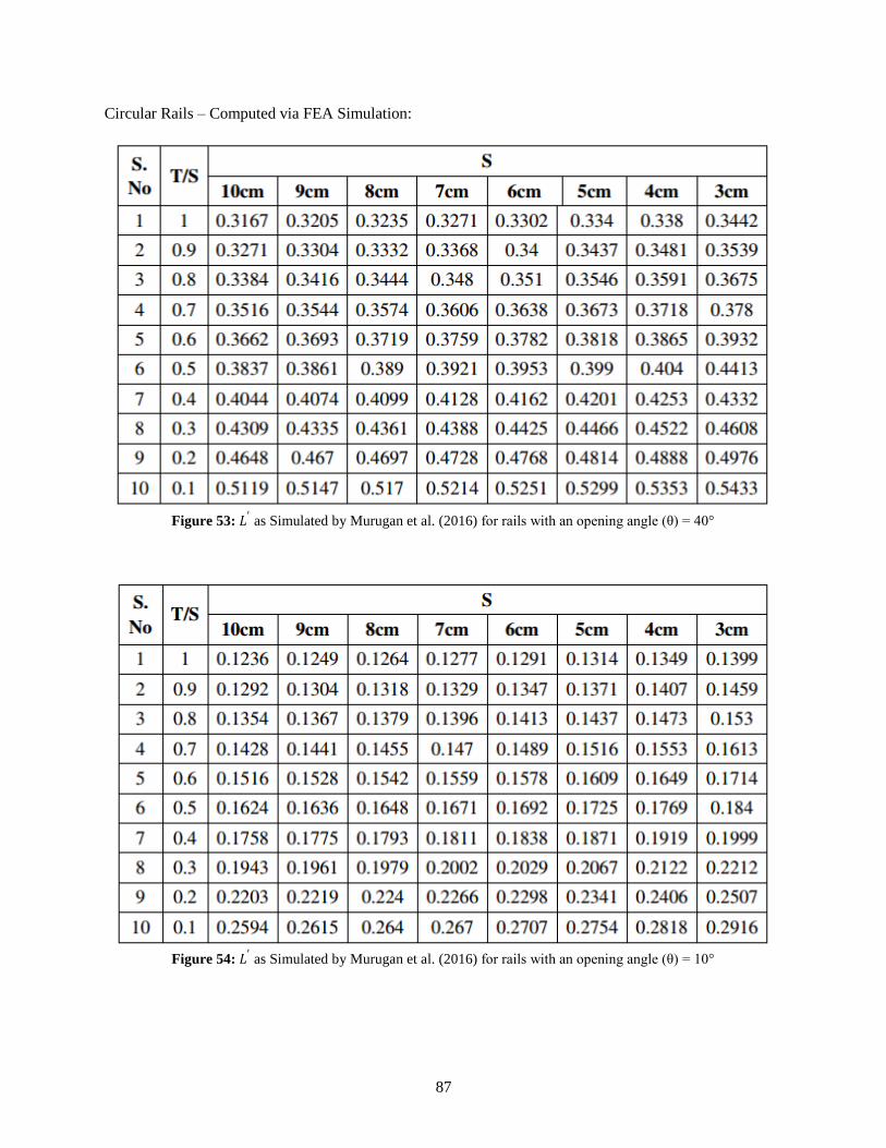
Figure 54 119871prime as Simulated by Murugan et al (2016) for rails with an opening angle (θ) = 40deg 87
Figure 55 119871prime as Simulated by Murugan et al (2016) for rails with an opening angle (θ) = 10deg 87
Figure 56 119871prime as Simulated by Bayati and Keshtkar (2013) 88
Figure 57 Replication of Figure 9 by Kerrisk (1982) 89
Figure 58 Replication of Figure 10 by Kerrisk (1982) 89
Figure 59 Replication of Figure 12 by Kerrisk (1982) 90
Figure 60 Replication of Figure 5 by Keshtkar Bayati and Keshtkar (2009) 90
Figure 61 Replication of Figure 6 by Keshtkar Bayati and Keshtkar (2009) 91
Figure 62 Replication of Figure 7 by Keshtkar Bayati and Keshtkar (2009) 91
xi
Nomenclature
119909 119910 119911 = position of point outside the rail
119909rsquo 119910rsquo 119911rsquo = position of point inside the rail
119897 = armature position [119898]
119898 = armature mass [kg]
119908 = rail width [119898]
ℎ = rail height [119898]
119904 = rail separation [119898]
120579 = rail opening angle for circular rails [119898]
119905ℎ = rail thickness for circular rails [119898]
119908119886 = armature width [119898]
ℎ119886 = armature height [119898]
119905119886 = armature thickness (size in z direction) [119898]
119868 = current [119860]
119868119875 = peak current [119860]
119868119905 = total current [119860]
119865 = Lorentz force on armature [119873]
119881 = armature velocity [119898119904]
119905 = time [s]
1199051 = current profile rise time [119904]
1199052 = current profile decline time [119904]
1199053 = current profile total time [119904]
119905119903119903 = rise time of current in the rails [119904]
119905119903119886 = rise time of current in the armature [119904]
119905119909 = time since current began flowing into the
conductor [119904]
119891 = frequency of a sign wave corresponding to
the current rise time in the rail [119867119911]
119891119886 = frequency of a sign wave corresponding to
the current rise time in the armature [119867119911]
120596 = frequency = 2 ∙ 120587 ∙ 119891 [119903119886119889]
120591 = capacitor time constant [119904]
120583 = material magnetic permeability [119867119898]
120583119903 = material relative permeability [~]
1205830 = magnetic permeability of free space
= 4πx10-7 [119867119898]
119890 = material permittivity of the dielectric
[119865119898]
1198900 = permittivity of free space
= 8854x10-12 [119865119898]
119890119903 = material relative permittivity [~]
119867 = magnetic field intensity [119860119898]
119869 = current density [1198601198982]
1198690 = current density in the conductor surface
119863 = electric flux density [1198621198982 ]
119864 = electric field intensity [119881119898]
119861 = magnetic flux density [1198821198871198982 ]
119860 = magnetic vector potential [119882119887119898]
Υ = electric scalar potential (voltage) [119881]
120588119907 = volumetric charge density [1198621198983 ]
120590 = material electric conductivity [119878119898]
119896 = thermal conductivity [119882(119898 ∙ 119870)]
119888119901 = material specific heat
119886 = distance from current flow to point of
interest (119903 to 119903prime) [119898]
119870119890 = sawtooth wave to sine wave comparability
index set to 1 [~]
120575119881 = skin depth considering VSE [119898]
120575119860119862 = skin depth of alternating current [119898]
120588119903 = material resistivity
= 177x10-8 [Ω sdot 119898]
119879 = temperature [119870]
1198790 = initial temperature [119870]
119879119898119890119897119905 = material melting temperature [119870]
() = equation number [~]
1
Chapter 1 Railgun Background
Railguns utilize a pair of conducting rails and a sliding armature which connects the two rails to
exploit the Lorentz force Current is sent down one rail through the armature and back through the other
rail The current flowing through the parallel rails creates a magnetic field around each rail and this
magnetic field interacts with the current flowing through the armature to create a Lorentz force as shown
in Figure 1
Electromagnetic launchers specifically railguns are an increasingly popular topic of interest from
both military and scientific communities for their ability to accelerate projectiles to high speeds (gt 5 kms)
(Poniaev et al 2016) (Meinel 2007) After being first investigated and constructed in the early 1900rsquos by
Kristian Birkeland (Coffo 2011) (Rice et al 1982) railgun research was declared unlikely to be successful
by US Air Force scientists in 1957 However research was reinvigorated following work by Richard
Marshall in 1977 who accelerated a 3g projectile to 59 kms using a 5 m long railgun and a 550 MJ
homopolar generator (Meinel 2007) After Marshallrsquos experiment railguns have been studied by the United
States military since before 1984 (DrsquoAoust et al 1984) and as a means for space launch by NASA since at
least 1982 (Rice et al 1982) (Turman and Lipinski 1996) Today (since at least 2003) the US Navy has
been researching railguns as a shipboard weapon (Lynn et al 2011) (McFarland and McNab 2003) and
interest in railguns as a means for space launch continues (McNab 2003) (Lehmann et al 2007) In 2005
James Brady examined the use of railguns as infantry weapons In 2008 and again in 2009 Ian McNab
reviewed the work being done by the University of Texas University of Minnesota University of New
Figure 1 Railgun Concept
Bore
2
Orleans and Texas Tech University on launching a space-bound payload from a high-altitude aircraft In
2008 NASA examined the use of an electromagnetic launcher to accelerate a scramjet to operating velocity
(around Mach 4 or 14 kms at sea level) The scramjet would take a payload to the upper atmosphere
where a small rocket would then launch the payload off of the scramjet and into orbit (Jayawant 2008)
This launcher discussed by NASA is not a railgun but rather a form of magnetic levitation powered by
linear induction motors Railguns in their most common form can produce accelerations in excess of
10000 gees (Meger et al 2013) (McFarland and McNab 2003) and it is speculated that because humans
and delicate hardware cannot survive this NASA has selected a less strenuous approach for launch
For military applications railguns represent an accurate low cost long range weapon that
introduces less vulnerability than traditional long range cannons (McFarland and McNab 2003) and have
been proposed as shore-barrage cannons and as anti-missile defense weapons A comparison of
conventional guns and proposed European and US shipboard railguns is presented in Table 1 using data
from Hudertmark and Lancelle (European) in 2015 and McFarland and McNab (USA) in 2003
Table 1 Railgun Performance vs Conventional Gun Performance (Modele 68 and Oto-Melara) where the USA
railgun data comes from McFarland and McNab (2003) and other data comes from Hudertmark and Lancelle (2015)
As shown here railgun ranges far exceed those of traditional guns due to the vast difference in
muzzle velocity Long range missiles can exceed the listed railgun ranges but are more expensive The
destructive energy of a railgun round comes from the kinetic impact of a 1-25 kms projectile (McFarland
and McNab 2003) instead of an explosive charge resulting in a cheaper round The high velocity of a
railgun round also reduces travel time increasing accuracy In addition because there is no longer need for
Proposed USA
Railgun
Proposed European
Railgun
Modele 68
(French)
Oto-Melara
(German)
Range [km] 300 - 500 up to 500 lt 17 20-30
Muzzle Velocity [ms] 2000 2500 870 925
Projectile Mass [kg] 164 5 13 5-6
Round Mass [kg] 219 8 23 12
Projectile-to-Round Ratio 749 625 565 417 - 50
Rate of Fire [rdsmin] 12 ~ 78 80
Round Cost [$1000] 5-10 ~ ~ ~
Barrel Length [m] 877 64 55 472
Bore Size [mm] 146 100 100 76
3
chemical propellant non-projectile mass and volume can be reduced though a railgun will require a large
power supply The removal of explosives also makes ships less vulnerable because there is much less
explosive material held onboard (McFarland and McNab 2003) (Meger et al 2013)
With regard to space launch only the most rigid payloads would be able to survive the launch loads
in current railguns But for these payloads railguns offer improved predictability improved efficiency and
reduced cost over rocket launch systems and would not require the use of environmentally harmful rocket
fuel Rocket performance is inherently reliant on the complex burning of solid fuel and the complex flow
of heated propellant The complexity of the constitutive processes involved in rocket engine operation and
the number of parts involved necessitate extensive testing (Freeman 2015) This not only results in high
monetary costs but significantly extends the time needed to provide new rockets Additionally rockets are
required to lift all needed propellant meaning much of the energy expended in rocket launch is only needed
to lift more fuel Railguns could be more affordable as they would require less testing (once developed)
and would not need to launch nearly as much non-payload mass For example sending 1 kg to low Earth
orbit cost around $22000 with the space shuttle (McNab 2003) $2700 with the more recent Falcon 9 and
the expected cost with the Falcon Heavy is $1700 per kg (SpaceX 2017) Railgun designs have suggested
prices could be reduced to around $600 per kg (McNab 2003) and railguns would not require the same
large scale that brings down the price per kg in the Falcon Heavy
Military railguns have very specific size and power requirements as they are intended to be
mounted on ships (Lynn et al 2011) Research railguns are generally similar with less focus on size
However in order to use railguns as a means for space launch significant changes must be made to standard
designs Primarily space launch payloads are much more massive (hundreds of kg compared to lt 5 kg)
and to achieve ballistic launch into orbit payloads must accelerate to very high velocities (~75 kms) To
keep accelerations reasonably low (~2000 gees) for rigid payloads the rails would need to be extended
from less than 10 m (Hudertmark and Lancelle 2015) (Lehmann 2003) in current railguns to 1500 m or
greater (McNab 2003) The transport of humans or other delicate hardware is much more difficult as
4
acceleration would need to reduce to ~3 gees meaning the minimum rail length needed to accelerate to 75
kms is 9375 km
Inspired by the active interest in the field of electromagnetic launchers this work examines the
presence of railgun modeling methods which are reasonably accurate but do not require the solution of
partial differential equations or the use of finite element methods Such methods would assist in simpler
computation of medium-fidelity models and design space exploration Simple reasonably accurate
methods of computing current profiles and inductance gradient values already exist and are applied and
examined here No readily applicable method of defining current distribution has been found so the
principles of current flow are defined and a rudimentary method is proposed A method for defining the
magnetic field in the armature has been mentioned by Xu and Geng (2010) but has not been explored at
length so two versions of this method are compared to finite element results to determine accuracy Two
readily applicable force equations exist the traditional ldquorailgun force equationrdquo and one defined by
Waindok and Piekielny (2016) This examination looks at the accuracy of these methods by comparing
them to four versions of a force equation defined by Xu and Geng (2010) finite element methods and
experimental methods to determine if accuracy improvements can be obtained by a more detailed analysis
Lastly a method for computing temperature in the rails proposed by McCorkle and Bahder (2010) is
replicated to confirm its operation In these models only solid rectangular armatures are considered so
significant adjustments may be necessary to account for plasma or brush armatures and different rail
armature geometries The examination of these methods informs decisions on their accuracy and assists in
preliminary railgun modeling Using methods which do not require the solution of partial differential
equations (and are all implemented with MATLAB here) opens the door for analysis by investigators with
little railgun experience Also aiding in this goal is an overview of the main factors important to railgun
operation and an introduction to the analysis of these factors presented here
5
Chapter 2 Power Supply Mechanisms
To model nearly all railgun factors it is necessary to know the applied excitation current For
transient analyses the time dependence of this current must be defined This section focuses on this
definition and presents a commonly used model for approximating current profiles Though most railgun
power supplies provide similar current pulses railgun power supply technologies are also described here to
provide background
Railgun power supplies must be able to provide pulses of high current over a few ms (around 1 to
15 ms) (Chengxue et al 2014) (Waindok and Piekielny 2016) (Stefani et al 2007) (Coffo 2011) (DrsquoAoust
et al 1984) (Murugan Kumar and Raj 2016) Many pulsed power systems exist though the most popular
for this application are Pulse Forming Networks (PFNrsquos) with capacitors and rotating machines (pulsed
homopolar generators rectified pulsed alternators and compulsators) (McNab 1997) (Lynn et al 2011)
(McNab 2003) (McFarland and McNab 2003) (DrsquoAoust et al 1984) (Meger et al 2013) As discussed by
McNab (2014) other possible techniques include flux compressors (Goldman et al 1999) (Li et al 2004)
magnetohydrodynamic (MHD) generators (Ying et al 2004) and pulsed inductors (Sitzman et al 2006)
(Liang et al 2016) (Meger et al 2013) Despite the many options for pulsed power Richard Marshall (the
head of the team responsible for reinvigorating railgun research in the late 1970rsquos) said in a 2001 article
that power supplies constitute the most concerning barrier to further railgun development
The simplest railgun power source would be a single large capacitor as capacitors are inherently
good at providing large current pulses over short periods of time However even if a very large single
capacitor (or single capacitor bank) is used current is only supplied for a very short amount of time without
further power conditioning and the amount of force provided would be too small For example a
hypothetical capacitor capable of supplying 300 kA with a time constant (τ) of 05 ms would only produce
current above 270 kA for 02 ms (obtained with the traditional discharging capacitor equation) To obtain
more time at high current and somewhat decrease the need for exceptionally high current pulses networks
of energy storage devices are used where the storage devices are linked with inductors in a Pulse Forming
6
Network (PFN) to spread out the current pulse
Though the most common storage devices are
capacitors other forms of energy storage can be used
such as transmission lines inductors (Haddad and
Warne 2004) or rotating machines (Lynn et al
2011) An example of a relatively simple PFN using
capacitors can be seen in Figure 2 from Gully et al
who sought to minimize PFN weight (Gully et al
1993)
Despite the various available options for railgun power supplies a common current profile is used
in the literature Generally the current profile is defined by a rapid rise ndash constant ndash slow set behavior (Xu
and Geng 2010) though it is not uncommon for researchers to simply assume constant current (McCorkle
and Bahder 2010) as most current (and thus force) flows in the ldquoconstantrdquo section
The current rise is sometimes modeled with a linear increase (Chengxue et al 2014) (Jin et al
2015) (Murugan Kumar and Raj 2016) but is more accurately modeled as the first quarter of a sign wave
as described by (1) where the harmonic frequency (120596) is defined by the rise time (1199051) as shown in ) (Xu
and Geng 2010) This rapid increase mirrors the description of AC current profiles and becomes
responsible for skin effects present in the rails as discussed more in the current distribution chapter The
second ldquoconstantrdquo section is simply described by (2) and the last ldquoslow setrdquo section is described by an
exponential decay in (3)
(1) 119868 = 1198680 ∙ 119904119894119899(120596 ∙ 119905) = 1198680 ∙ 119904119894119899 (120587
2 1199051 ∙ 119905) ( 0 le 119905 le 1199051 )
(2) 119868 asymp 1198680 ( 1199051 le 119905 le 1199052 )
(3) 119868 = 1198680 ∙ 119890minus119905 120591frasl
( 1199052 le 119905 le 1199053 )
(4) 120596 = 2 120587 ∙ 119891 119908ℎ119890119903119890 119891 = 1
4 1199051 rarr 120596 =
120587
2 1199051
Figure 2 Pulse forming network schematic (Gully
et al 1993)
7
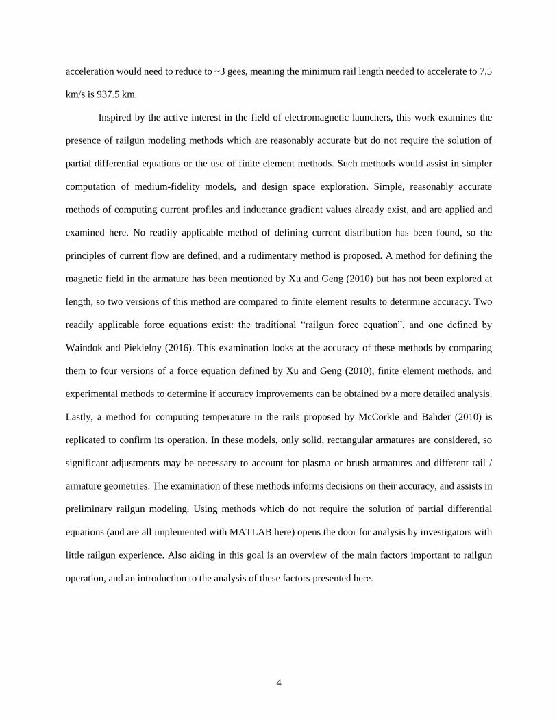
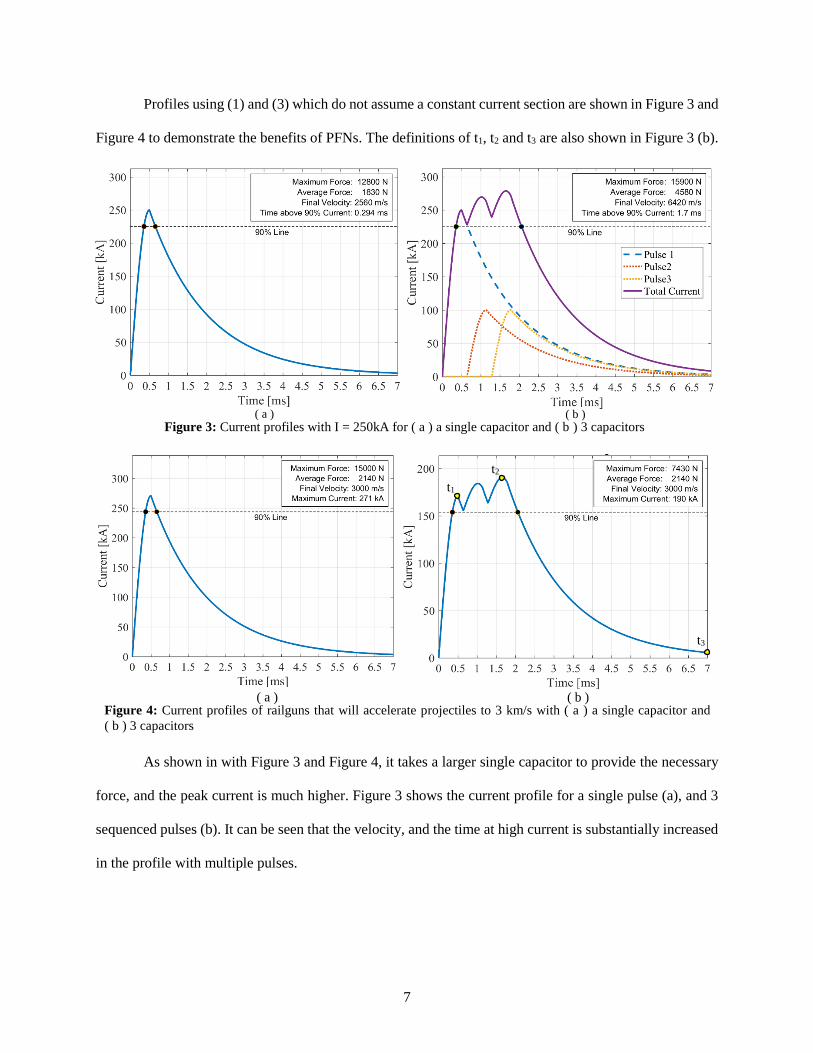
Profiles using (1) and (3) which do not assume a constant current section are shown in Figure 3 and
Figure 4 to demonstrate the benefits of PFNs The definitions of t1 t2 and t3 are also shown in Figure 3 (b)
As shown in with Figure 3 and Figure 4 it takes a larger single capacitor to provide the necessary
force and the peak current is much higher Figure 3 shows the current profile for a single pulse (a) and 3
sequenced pulses (b) It can be seen that the velocity and the time at high current is substantially increased
in the profile with multiple pulses
( a ) ( b ) Figure 4 Current profiles of railguns that will accelerate projectiles to 3 kms with ( a ) a single capacitor and
( b ) 3 capacitors
t3
t2
t1
( a ) ( b ) Figure 3 Current profiles with I = 250kA for ( a ) a single capacitor and ( b ) 3 capacitors
8
The force and velocity for each profile is found using the railgun force equation (5) and assumes a
maximum current of 250 kA an 119871prime of 041 μHm and a projectile mass of 5 g
(5) F =119871prime ∙ 119868(119905)2
2
The ldquo90 linerdquo is found by comparing the provided current with the maximum current of the first
larger capacitor In the hypothetical group of sequenced capacitors used here the first capacitor provides
250 kA and the latter ones provide 100 kA It is not surprising that more capacitors yield more velocity
but the particular advantage of a PFN can be seen with Figure 3 In the first profile (a) a projectile is
accelerated to 3 kms with a single capacitor using a peak current of 2706 kA In (b) the projectile is
accelerated to 3 kms with 3 capacitors using currents of 1709 kA 6836 kA and 6836 kA Therefore a
single capacitor needs to reach a much higher current to accelerate its projectile to 3000 ms Higher current
spikes mean more issues with temperature rise and this short acceleration time means the payload is subject
to much higher launch loads Additionally the temperature increases that come with higher current spikes
cause the railgun resistance to increase as well meaning the disparity between PFNrsquos and individual
capacitors would be greater if this effect was considered and the single capacitor profile would be less
efficient
Three experimental current profiles are provided in Figure 5 on the following page for qualitative
comparison (Meger et al 2013) (Lehmann et al 2007) (Schneider et al 2009 pt2) (Stefani et al 2007) It
can be seen that the average current in the ldquoconstantrdquo section is relatively constant in (a) (b) and (d) but
there are still significant departures from constant current in (b) and (c) The assumption of constant current
remains an idealization but it does have empirical backing
9
21 Capacitor Banks
Capacitor banks have been the most common railgun power source as the technology is well developed
reliable and relatively simple (Meinel 2007) (McNab 1997) (Lynn et al 2011) (McNab 2003) (McFarland
and McNab 2003) (DrsquoAoust et al 1984) (Meger et al 2013) (Lehmann et al 2007) The PFN that powers
the PEGASUS railgun installed at the Institute of Saint-Louis (ISL) utilizes capacitor banks to provide a
current pulse around 600 kA for nearly 15 ms
(Figure 5 (b) and Figure 6) (Lehmann et al 2007)
(Spahn and Buderer 1999) Individually simple
capacitor banks still provide relatively short current
pulses It is only with the addition of power
conditioning through inductors and crowbar diodes
that these extended pulses can be obtained Figure 6 The PEGASUS railgun at ISL and part of the
capacitor bank that powers it (Lehmann et al 2007)
( c ) ( d )
( a ) ( b )
Figure 5 Experimental current profiles supplied by (a) power supplied to the railgun at MTF using 22
capacitor banks with 500kJ capacity each (Meger et al 2013) (b) power supplied to the PEGASUS railgun
at ISL using a capacitor bank of 200 modules with a capacity of 50kJ each (Lehmann et al 2007) (c) power
supplied to the RAFIRA railgun at ISL using 9 of 20 available capacitor banks (Schneider et al 2009 pt2)
(d) power supplied to the HEMCL railgun at IAT power supply consists of 18 banks of 24 capacitors each
(Stefani et al 2007) (Watt 2011)
10
Capacitor banks can be modular (Baker et al 1989) and therefore allow for relatively simple maintenance
when needed But the ability to adjust their operation without adding or replacing components is very
limited in comparison to other systems (Gao et al 2015) Due to the number of relatively large physical
components needed to network capacitors banks are generally heavy and physically large (low energy
density) compared to other energy storage methods though work to reduce capacitor bank size is ongoing
(Liu et al 2011) This is the main reason capacitor banks are not the favored choice for military shipboard
systems despite the fact that they are static and thus do not produce large torques like rotating machines
(McFarland and McNab 2003) However mass and volume are less of a concern for research laboratories
and prospective space launch systems making capacitor banks the preferred choice for many stationary
railgun systems
22 Rotating Machines
In early railguns the rotating machines used were homopolar generators (HPGs) (Marshall 2001) HPGs
once started with an excitation current (usually provided by an inductor) rotate a conductive disk in a
magnetic field producing a Lorentz force pointed toward the edge of the spinning disk The current
produced from the rotating disk is collected withh brushes (sliding contact) around the disk edge This
method allows large currents to be generated for short periods However according to McNab (2014) HPGs
have inherent issues with
Wear and maintenance due to a reliance on sliding contacts
Providing for multiple shot operation due to switching difficulties
Obtaining high energy density due to tip speed limits from the use of ferromagnetic materials
Attention then switched in the 1990s and 2000s to rectified pulsed alternators especially for military
applications (McFarland and McNab 2003) (Gao et al 2015) (Meger et al 2013) (Walls et al 1997) Pulsed
alternators use excited rotor windings on the face of the rotating mass to excite stator windings which then
deliver output power The alternator pulse width is small compared to that needed by railguns so multiple
11
smaller pulses are delivered resulting
in a similar current profile to PFNs
using capacitors (Figure 7) A variant
of pulsed alternators uses winding
compensation to reduce impedance
and increase output current These are
commonly referred to as
compulsators and have been under ongoing research for over 30 years (Gao et al 2015) (Pratap et al 1984)
(Gully 1991) (Pratap and Driga 1999) (Marshall 2001) The main advantage of pulsed alternators is that
they operate with lower current allowing multiple windings and thus multiple poles which enables higher
voltage power than HPGrsquos Other advantages include a freedom from sliding contacts the ability to store
and deliver energy for multiple shots and a deep history of research due to the similarity to synchronous
AC generators used by utility companies A list given by McNab (2014) describes the remaining issues
with pulsed alternators as being
manufacturing complexity introduced by the need for tight tolerances
thermal management in the rotor windings
output pulse rectification due to their inherent AC nature
the size and capacity of switching and control devices
multimachine synchronization
efficiency
cost
Additionally as reported by Pratap et al electrical forces in compulsator rotor windings attempt to peel the
winding from the rotor surface adding to the structural and material demands on the rotor (Pratap and Driga
1999) Even though issues with cost and efficiency are likely not specific to pulsed alternators a suggestion
Figure 7 Compulsator current profile (McNab 2014)
12
by McNab and recent research by Engel et al suggests that interest may be returning to HPG research
(Marshall 2001) (Pratap and Driga 1999) (McNab 2014)
Advantages with rotating machines in general in addition to their previously mentioned energy
density consist of flexibility (Gao et al 2015) and longer life expectancies (Hebner et al 2006) General
disadvantages with rotating machines are that they produce an external torque when discharging meaning
they must be used in pairs on ship-board railguns and they are much more mechanically complex than
capacitor systems If maintenance is required the whole generator has to be shut down or replaced unlike
capacitor systems Lastly the usage of kinetic energy storage (large flywheels spinning at thousands of
RPM) introduces some risk for ship-based systems in the event of attack
13
Chapter 3 Current Distribution
With the supply current defined it is then necessary to examine how current distributes in the rail
and armature This is important as current concentrations create excessive heating and the current
distribution partially dictates the railgun force Heating is problematic since it increases electrical resistance
and causes rail damage The Lorentz force depends on the interaction of current and magnetic field so
maximizing force relies on regions of high current coinciding with regions of high magnetic field The work
in this chapter describes the main principles of current distribution relevant to railguns and presents a
rudimentary method to estimate it for railguns with solid rails and rectangular armatures
Current distribution is one of the most complex analyses necessary for describing railgun operation
since it is entirely dependent on the solution of partial differential equations The relevant equations for this
analysis are Maxwellrsquos equations (6) rarr (8) along with the charge continuity equation (10) five constitutive
equations (11) rarr (15) and the relations of (16) and (17) (Zhao et al 2014) As shown by Zhao et al (2014)
current density can be described by (18) rarr (20) where (19) and (20) must be solved simultaneously
(6) nablatimes119815 = 119817 + part119811
partt (7) nablatimes119812 = minus
part119809
partt
(8) nabla ∙ 119915 = 120588119881 (9) nabla ∙ 119913 = 0
(10) nabla ∙ 119921 = minus part120588119881
part119905
(11) 119913 = 120583119919 (12) 119915 = 휀119916
(13) 119921 = 120590119916 (14) 120583 = 1205830120583119903
(15) 휀 = 휀0휀119903
(16) 119916 = minusnablaΥ minus part119912
partt (17) 119913 = nabla times 119912
(18) 119921 = 120590 (minusnablaΥ minus part119912
partt)
(19) 120590part119912
partt+1
1205830[nablatimes(nablatimes119808) ] + 120590nablaΥ = 0
(20) nabla ∙ (120590nablaΥ) = 0
(21) nabla ∙ (120590nablaΥ + 120590part119912
partt) = 0
14
The formulation used by Zhao et al assumes the following
All materials are isotropic and non-ferromagnetic
o As a result the relative magnetic permeability (microR) for all materials is 1 This assumption
is reasonable because most railguns are composed mainly of copper rails and an aluminum
armature both of which have a relative permeability close to 1
Quasi-static operation
o This allows the displacement current term ( part119915
part119905 ) to be neglected in (6) as has been done
before in railgun analysis (Kerrisk 1982)
The change in magnetic vector potential ( part119912
partt ) from (16) is 0 when deriving (20)
o If this assumption is not made (13) and (16) can be combined with a finding by Zhao et
al that partρV
partt= 0 can be written giving nabla ∙ 119817 = 0 In this case (20) would look like (21)
Equations (18) rarr (20) were defined utilizing these assumptions It is now necessary to explore the nuances
and consequences of rail current distribution
Areas of high current density are of particular interest in railgun design as these areas are prone to
excessive Joule heating and dictate the magnetic field shape In simple railgun operation the vast majority
of the current flows through a thin layer near the rail surface This is due to five main factors Of these the
skin effect of alternating current and proximity effect are commonly present in stationary conductors with
AC power Much of the following description is compiled from the work of Lv et al (2014) from the
Chinese Shijiazhuang Mechanical Engineering College
Clustering Near Small Source of Constant Current (CNSS) (Lv et al 2014)
Clustering Along Short Path of Constant Current (CASP) (Lv et al 2014)
Proximity Effect (Lou et al 2016)
Skin Effect of Alternating Current (SAC) (Lv et al 2014)
Velocity Skin Effect (VSE) (Lv et al 2014) (Lou et al 2016)
15
These factors are described below as many railguns use the ldquosimple railgunrdquo design with solid rails
However much of the concern with current distribution in rails has been solved by using laminated rails
which use thin strips of rail material separated by dielectric Using thin strips reduces the impact of the skin
effect since the whole strip cross-section is essentially ldquoskinrdquo This means that approximating the current
distribution as uniform is reasonably accurate for laminated rails (Xu and Geng 2010) (Xing et al 2015)
Thus the bulk of this analysis assumes a uniform current distribution in the rails though it is true that near
the armature current will still concentrate along the rail inner face
31 Clustering Near Small Source (CNSS)
The first of these (CNSS) simply acknowledges that when a current spot source spot sink exists
current concentrates around this point The relationship of current density (119921) to position around this spot is
described by (22) whereas the relationship around a line-like source is described by (23)
(22) 119869(119903) prop 1198690
1199032 (23) 119869(119903) prop
1198690
119903
Here r is the distance from the spot and 1198690 is the current density in the spot source or sink This effect is
most relevant to the current density in the armature and rail along the contact surface On a large and
medium scale the rail can be thought of as a line-source and the vertical trailing edge of the armature can
be thought of as a line-sink (due to CASP) On a small scale regions of actual contact between rail and
armature can be thought of as spot sources (Figure 8) The presence of these current concentrations serve
to exacerbate issues of armature heating rail wear and transition
Figure 8 Current flow through imperfect electrical contact (Kim Hsieh and Bostick 1999)
16
32 Clustering Along Short Path (CASP)
The second effect (CASP) describes the fact that current will concentrate along the shortest path
between high and low voltage locations This effect can be recognized easily with (24) where a reduction
in path length ( int 119889119897 ) will result in an increase in current density ( 119921 ) for a given voltage
(24) Υ = int120588 ∙ 119921 119889119897
It should be noted that in a railgun application (24) will use different densities to account for the different
material in rail and armature In the simple railgun this effect causes the current to concentrate along planes
2 4 and 6 as shown in Figure 9
33 Proximity Effect
The proximity effect as described by Pagnetti et al is generated by current-carrying conductors
being nearby (within distances that are on the order of the conductor radius) A conductor in this case will
induce eddy currents that alter the internal impedance of nearby conductors resulting in current
concentration on the side of the responsible conductor (Pagnetti et al 2011) The proximity effect was
studied in railguns in 2016 by Lou et al and like the skin effect depends on frequency (rise speed) The
proximity effect (as its name suggests) is dependent on the rail separation (119904) A decrease in 119904 will increase
the effect and an increase in 119904 will make the effect fall off The proximity effect was shown to be invariant
with changes in current amplitude There is not yet any simplified analytical method to quantify this effect
but analysis with the partial differential equations listed above will inherently consider it (Lou et al 2016)
The result of these findings is an additional motivation to keep railgun rails at a healthy distance from each
Figure 9 Railgun concept considering CASP with planes 1 rarr 7 defined for reference
17
other as this will reduce current concentration Increasing rail separation also yields improvements in 119871prime
resistance and rail stress (Lou et al 2016) (Keshtkar 2005) (Xu and Geng 2010)
34 Skin Effect of Alternating Current (SAC)
The fourth effect commonly called the skin effect becomes significant when rapidly changing
current (usually in alternating current applications) is applied to a conductor In such cases the current
concentrates around the conductor surface (Thomas and Meadows 1985) Though railguns operate on DC
power the rapid rise of the current pulse (from 119905 = 0 to 119905 = 1199051 in Figure 3 (b)) induces the same effect In
fact Lv et al argue that the amount of current in the rail center is negligible and therefore use an equivalent
hollow rail to perform their analysis (Lv et al 2014) to model the skin effect without using a transient finite
element solution
The current distribution in a large conducting plane is described by (25) which can be broadly
simplified to (26) Both equations depend on the AC skin depth which has many equivalent definitions
Three of these are shown in (27)
(25) 119869 = 1198690 ∙ 119890( minus119909prime
120575119860119862) ∙ 119890119869 ∙ (
119909prime
120575119860119862 minus 120596 ∙ 119905119903119903)
(26) 119869 = 1198690 ∙ 119890( minus119909prime
120575119860119862)
(27) 120575119860119862 = radic2 ∙ 120588119903
120596 ∙ 120583= radic
120588119903
120587 ∙ 119891119903 ∙ 120583= radic
4 ∙ 119905119909
120590 ∙ 1205830
119908ℎ119890119903119890 119909prime = 0 119886119905 119905ℎ119890 119888119900119899119889119906119888119905119900119903 119904119906119903119891119886119888119890 ℎ119890119903119890 119886119899119889
119890119869 ∙ ( 119909prime
120575119860119862 minus 120596 ∙ 119905)
= electromagnetic fluctuation coefficient
119890( minus119909prime
120575119860119862) = damping coefficient
18
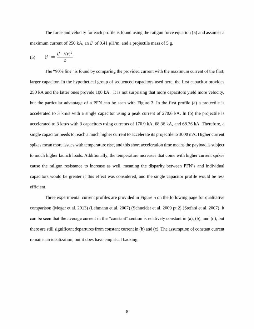
Each of these equations assume that the current flows through a good conductor which applies for
copper and aluminum This skin effect is responsible for a significant amount of the current concentration
that produces melting in the armature and solid rails It also seems to be responsible for the greatest current
concentration being at the top and bottom of the rail inner surface (shown in Figure 10 and Figure 11) as
the shortest path for the current flowing along the top bottom and outer surfaces is through these corners
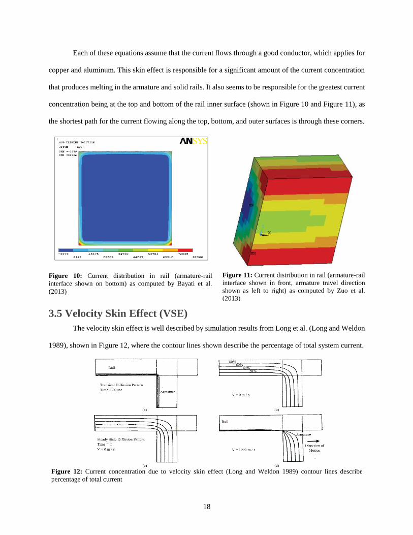
35 Velocity Skin Effect (VSE)
The velocity skin effect is well described by simulation results from Long et al (Long and Weldon
1989) shown in Figure 12 where the contour lines shown describe the percentage of total system current
Figure 10 Current distribution in rail (armature-rail
interface shown on bottom) as computed by Bayati et al
(2013)
Figure 11 Current distribution in rail (armature-rail
interface shown in front armature travel direction
shown as left to right) as computed by Zuo et al
(2013)
Figure 12 Current concentration due to velocity skin effect (Long and Weldon 1989) contour lines describe
percentage of total current
19
It can be seen from (a) and (c) that if the armature is held in position the current will eventually
diffuse throughout the conductors The time necessary for this to happen is directly dependent on the
materialrsquos magnetic permeability electrical conductivity and the length of the diffusion distance (Long and
Weldon 1989) As the armature begins to travel current is passing through sections of rail that have not
been exposed to current flow This means that current does not have time to diffuse into a new arbitrary rail
section and current then concentrates on the surface of the rail at the trailing edge of the armature as shown
in (d)
Even if the velocity had no impact a railgun shot lasts far less than a second (commonly ~5 ms)
and the current would not have enough time to diffuse throughout the rail as shown in Figure 12 (a)
Regardless this effect remains significant in railguns because current concentrates more highly in faster
railguns and concentrates less in slower ones (Lv et al 2014)
An analytical description of this effect can be obtained by modifying (25) rarr (27) used for assessing
skin effect At the base of the rails (planes 1 and 7 from Figure 9) the frequency ( 119891119886 ) can be found by
considering the rise time (1199051) as one fourth of the period giving 119891119886 = 1
4lowast1199050 In an arbitrary rail section the
frequency has been described by the same general formula but with the time given by ∆119905 =119905119886
119881 where ta is
the length (or thickness) of the armature contact interface (planes 3 and 5) and 119881 is the armature velocity
The equation for time is obtained with the knowledge that the current density in an arbitrary rail section
increases from 0 to 119869119898119886119909 in the time it takes the armature to pass the rail section (Lv et al 2014) In reality
because of CASP most of the current flows through the trailing armature face (plane 4) so the majority of
this increase from 0 to 119869119898119886119909 happens when the last portion of the armature passes the rail section Thus a
more accurate computation of frequency would come from defining an equivalent rise time that accounts
for this exponential behavior This computation is not performed here but a factor of 1
2 is applied because
it is safe to say that the vast majority of the current flows through the trailing half of the armature
The final 120549119905 and 119891119886 equations are therefore given by (28) and (29) and the velocity skin depth (the
depth into the conductor that current flows) is given by (30)
20
(28) ∆119905 =119871119886
2 ∙ 119881
(29) 119891119886 = 1
4 ∙ ∆119905=
119881
2 ∙ 119871119886
(30) 120575119881 = 119896119890 ∙ radic4 ∙ 120588119903 ∙ 119905119903119886
120587 ∙ 120583 ∙ 119881= 119896119890 ∙ radic
2 ∙ 120588119903
120587 ∙ 120583 ∙ 119891119886
An additional approximation made by Lv et al assumes the period resulting from a linear increase
(equivalent to one quarter of a sawtooth wave period) can approximate the period of a sine wave A
comparability index ( 119896119890 ) is used to describe this but is set to unity It can be seen from (30) and (27) that
if the current rises faster the skin depth will decrease meaning the current is more concentrated and thus
produces more local Joule heating
36 Current Distribution Approximation (CStSM)
For this analysis current distribution in the rails is assumed to be uniform due to the advent of
laminated rails Regardless a rudimentary method for computing current distribution in solid rails and the
armature is presented This approximation is obtained by computing a distribution that is shaped roughly
correctly then scaled to represent the correct quantity of current This method will be called the CStSM
(Current Shape then Scale Method) for the purposes of this paper
The shape is defined using the skin depth and current density equations ((26) (27) and (30)) at
each point in the rail or armature In the rails this results in (31)
(31) 119921119894 119895 = 119890( minus119909119894prime
120575119860119862)+ 119890
( minus119910119895prime
120575119860119862)
1198690 is defined as 1 here because the magnitude will be defined later when the result is scaled
In the armature the current will only concentrate along the rear face (as dictated by CASP) and
thus the shape is defined by (32)
(32) 119921119895 119896 = 119890( minus ( 119911119896 minus 119897 )
120575119860119862)
21
Now that the shape is defined (in a 2D matrix for the rail and a 3D matrix that is uniform in the x and y
directions for the armature) the scaling factor (119878) must be computed This is done with the knowledge that
some total amount of current (119868119905) is flowing through any given area of interest and the current density must
reflect this First the total amount of current predicted initially (119868119894119899) must be found with (33) for the rail or
(34) for the armature then the ratio of the total current to the initially predicted current ( 119868119905119868119894frasl ) defines
the scaling factor
(33) 119868119894119899 = sum sum ( 119921119894 119895 ∙ 119889119909 ∙ 119889119910)119899
119895=1
119898
119894=1
(34) 119868119894119899 = sum sum ( 119921119895 119896 ∙ 119889119910prime ∙ 119889119911prime)
119901
119896=1
119899
119895=1
119882ℎ119890119903119890 119889119909 119889119910 119886119899119889 119889119911 119886119903119890 119905ℎ119890 119903119886119894119897 119892119903119894119889 119890119897119890119898119890119899119905 119908119894119889119905ℎ ℎ119890119894119892ℎ119905 119886119899119889 119889119890119901119905ℎ 119903119890119904119901119890119888119905119894119907119890119897119910
119886119899119889 119889119909prime 119889119910prime 119889119911prime119886119903119890 119905ℎ119890 119886119903119898119886119905119906119903119890 119892119903119894119889 119904119894119911119890119904 119886119899119889 119909 119886119899119889 119910 119886119903119890 0 119886119905 119905ℎ119890 119888119900119899119889119906119888119905119900119903 119904119906119903119891119886119888119890
The final current distribution is found by simply multiplying the current density by this scaling
factor In these equations the indices 119894 119895 and 119896 correspond to the 119909 119910 and 119911 directions Similarly the total
number of points in the 119909 119910 and 119911 directions are 119898 119899 and 119901
(35) 119878 = 119868119905
119868119894119899
22
37 CStSM Comparison
This method was applied to the case used by Lv et al (2014) to assess its accuracy The details of this
comparison case are shown in Table 2
Table 2 Railgun parameters used by Lv et al (Lv et al 2014) 119871prime was calculated not sourced directly
Lv et al performed their analysis using ANSYS Maxwell 140 and a mesh with a maximum element
dimension of 2 mm Two comparisons are made one for the armature and one for the rail current density
The armature comparison shows reasonably good agreement between the two results with some
obvious caveats The approximation made here does not consider any variation in current density along the
armature height This has two consequences First the CStSM results do not show higher current density
along the top and bottom edges like the ANSYS results do Second the peaks at the top and bottom corners
are not replicated since the density is not compounded by concentration at multiple edges This also means
the maximum 119869 in the ANSYS result is higher than in the CStSM result Regardless the average current
density along the armature rear face (left of Figure 13 (b) and Figure 14 (b) on the following page) is
~12x1010 [1198601198982frasl] in the ANSYS result and ~1x10¹⁰ [119860
1198982frasl] in the CStSM result giving the CStSM an error
of about -1667 relative to ANSYS The falloff looks to happen slightly more quickly with the CStSM
than ANSYS
Physical Parameters Symbol Value Value Symbol Electrical Parameters
Rail Length [m] L ~ 500 IP Peak Current [kA]
Rail Separation [m] s 004 005 t1 Current Profile Rise Time [ms]
Rail Width [m] w 001 005 t2 Current Profile Decline Time [ms]
Rail Height [m] h 004 01 t3 Current Profile Total Time [ms]
Inductance Gradient [microHm] 119871prime 05279 Value Symbol Material Parameters
Armature Width [m] wa 004 Cu ~ Rail Material [~]
Armature Height [m] ha 003 Al ~ Armature Material [~]
Armature Thickness [m] ta 002 4 E -8 120588119903 Armature Resistivity [Ωm]
Armature Velocity [ms] V 400 177E -8 120588119903 Rail Resistivity [Ωm]
23
The rail comparison is similar but the overall shape matches the ANSYS result better The shape
of the CStSM result does seem to have a thinner region of high current density though the colormap on the
CStSM result does drop to its darkest level a 1x10⁹ as opposed to 17x107 in the ANSYS result Both
computations predict higher current density along the rail inner face (on the right side in both plots) though
Figure 14 Current distribution in the ( a ) ndash rail 119909-119910 cross-section (bore to the right of the rail section) and
( b ) ndash armature-rail interface 119910-119911 cross-section (trailing edge of armature on the left) computed by the
CStSM in MATLAB The colorbar scale applies to both plots
( a ) ( b )
Figure 13 Current distribution in ( a ) ndash rail 119909-119910 cross-section (bore to the right of the rail section) and
( b ) ndash armature-rail interface 119910-119911 cross-section (trailing edge of armature on the left) (Lv et al 2014)
( a ) ( b )
24
this is more pronounced in the ANSYS result Both results predict a current density of about 3x10⁹ [1198601198982frasl]
along the top and bottom of the rail The maximum current density in both plots is at the top and bottom
corners along the rail inner face though this maximum is higher in the ANSYS result at ~12x1010 [1198601198982frasl]
compared to ~1x10¹⁰
This chapter has described the main principles behind current distribution in railguns proposed a
method to approximate this distribution and investigated its accuracy In the force computation two
methods (called F3 and F4) use the CStSM to find the current distribution in the armature The rest of this
paper (with the exception of some finite element 119861 field computations) assumes the use of laminated rails
so the CStSM is not used to compute current distribution in the rails Regardless the accuracy of this method
demonstrated here coupled with its ease of use compared to finite element solutions means it has promise
for use in medium-fidelity analyses and implementation in software packages like MATLAB
25
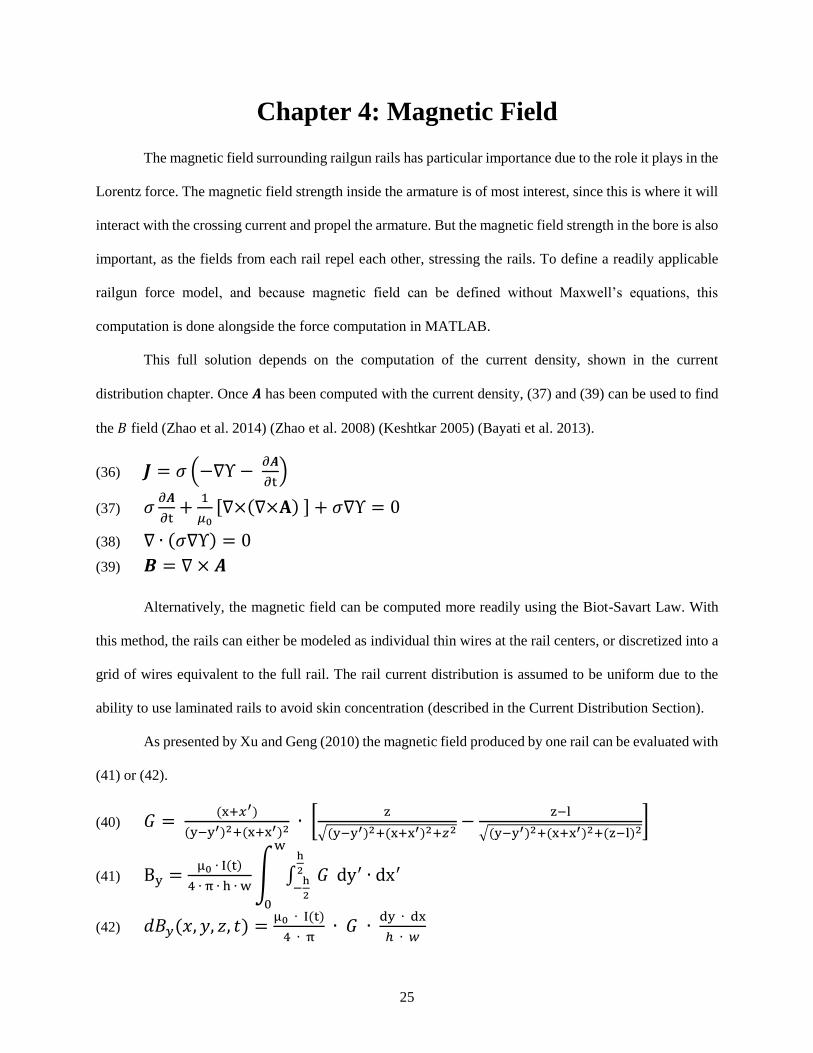
Chapter 4 Magnetic Field
The magnetic field surrounding railgun rails has particular importance due to the role it plays in the
Lorentz force The magnetic field strength inside the armature is of most interest since this is where it will
interact with the crossing current and propel the armature But the magnetic field strength in the bore is also
important as the fields from each rail repel each other stressing the rails To define a readily applicable
railgun force model and because magnetic field can be defined without Maxwellrsquos equations this
computation is done alongside the force computation in MATLAB
This full solution depends on the computation of the current density shown in the current
distribution chapter Once 119912 has been computed with the current density (37) and (39) can be used to find
the 119861 field (Zhao et al 2014) (Zhao et al 2008) (Keshtkar 2005) (Bayati et al 2013)
(36) 119921 = 120590 (minusnablaΥ minus part119912
partt)
(37) 120590part119912
partt+1
1205830[nablatimes(nablatimes119808) ] + 120590nablaΥ = 0
(38) nabla ∙ (120590nablaΥ) = 0
(39) 119913 = nabla times 119912
Alternatively the magnetic field can be computed more readily using the Biot-Savart Law With
this method the rails can either be modeled as individual thin wires at the rail centers or discretized into a
grid of wires equivalent to the full rail The rail current distribution is assumed to be uniform due to the
ability to use laminated rails to avoid skin concentration (described in the Current Distribution Section)
As presented by Xu and Geng (2010) the magnetic field produced by one rail can be evaluated with
(41) or (42)
(40) 119866 = (x+119909prime)
(yminusyprime)2+(x+xprime)2 ∙ [
z
radic(yminusyprime)2+(x+xprime)2+1199112minus
zminusl
radic(yminusyprime)2+(x+xprime)2+(zminusl)2]
(41) By =μ0 ∙ I(t)
4 ∙ π ∙ h ∙ wint int 119866
h
2
minush
2
dyprime
w
0
∙ dxprime
(42) 119889119861119910(119909 119910 119911 119905) =μ0 ∙ I(t)
4 ∙ π ∙ 119866 ∙
dy ∙ dx
ℎ ∙ 119908
26
These equations can be derived from the Biot-Savart Law for line conductors (43) which can be
simplified to (42) for a finite wire where 1205791 and 1205792 are defined in Figure 15 and 119903 and 119903prime are defined in
Figure 16 (Liao et al 2004)
(43) 119861 = μ0 4 ∙ π ∙ ∭ (
119921(119955prime) times (119955minus119955prime)
|119955minus119955prime|2 ) 119889119881
119881
(44) 1198621 = μ0 ∙ I(t)
4 ∙ π ∙ 119886 ∙ 119908
2
(45) 119861 = 1198621 ∙ int sin(120579) 119889120579 = 1205792minus1205791
μ0 ∙ I(t)
4 ∙ π ∙ 119887 ∙ ( cos(1205792) + cos(1205791) )
119908ℎ119890119903119890 119887 = 119886 + 119908
2
Figure 15 Rear view of the left rail current at 119903prime produces magnetic field at 119903
119903prime(119909prime 119910prime 119911prime)
119903(119909 119910 119911) 119887
x
y 119861
Figure 16 Biot-Savart variable definitions for both
thin-rail cases
(a) (b)
27
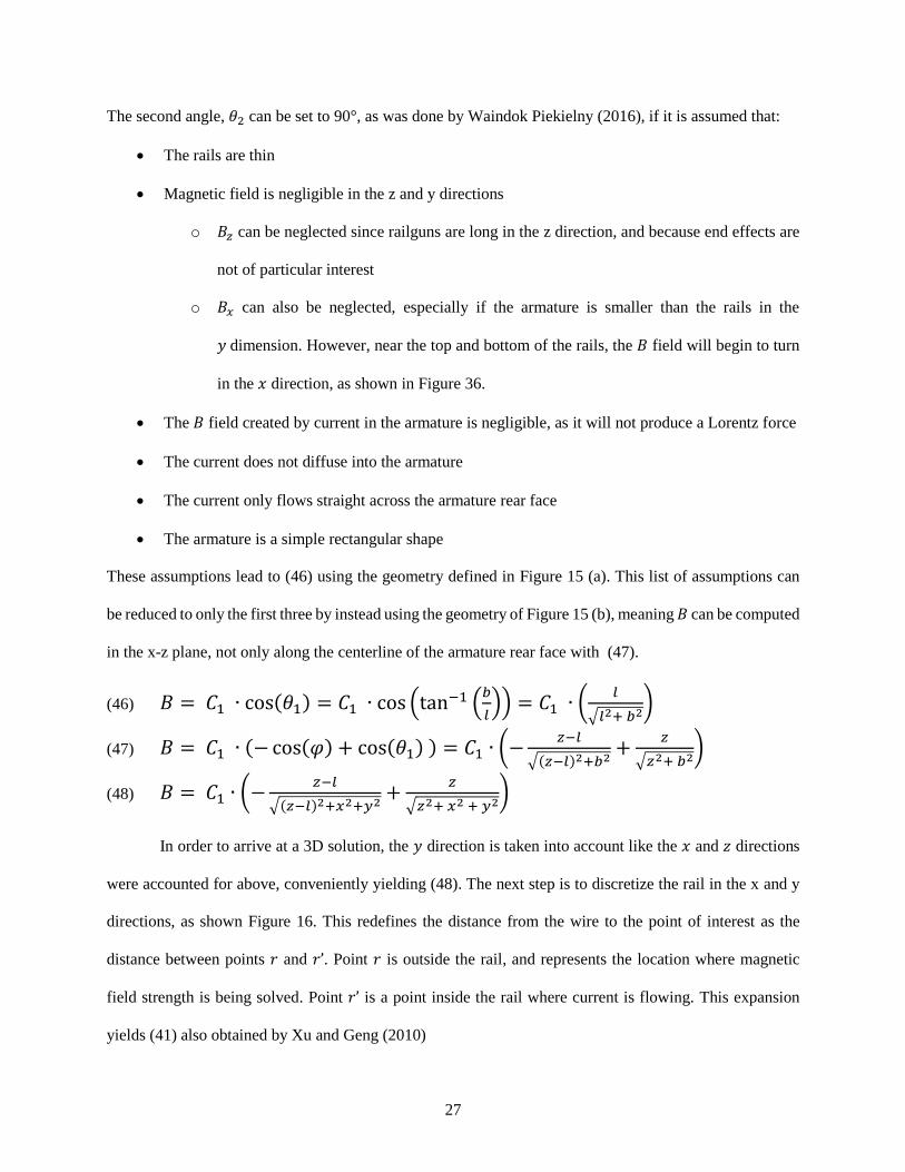
The second angle 1205792 can be set to 90deg as was done by Waindok Piekielny (2016) if it is assumed that
The rails are thin
Magnetic field is negligible in the z and y directions
o 119861119911 can be neglected since railguns are long in the z direction and because end effects are
not of particular interest
o 119861119909 can also be neglected especially if the armature is smaller than the rails in the
119910 dimension However near the top and bottom of the rails the 119861 field will begin to turn
in the 119909 direction as shown in Figure 36
The 119861 field created by current in the armature is negligible as it will not produce a Lorentz force
The current does not diffuse into the armature
The current only flows straight across the armature rear face
The armature is a simple rectangular shape
These assumptions lead to (46) using the geometry defined in Figure 15 (a) This list of assumptions can
be reduced to only the first three by instead using the geometry of Figure 15 (b) meaning 119861 can be computed
in the x-z plane not only along the centerline of the armature rear face with (47)
(46) 119861 = 1198621 ∙ cos(1205791) = 1198621 ∙ cos (tanminus1 (119887
119897)) = 1198621 ∙ (
119897
radic119897 2+ 1198872)
(47) 119861 = 1198621 ∙ (minus cos(120593) + cos(1205791) ) = 1198621 ∙ (minus119911minus119897
radic(119911minus119897)2+1198872+
119911
radic119911 2+ 1198872)
(48) 119861 = 1198621 ∙ (minus119911minus119897
radic(119911minus119897)2+1199092+1199102+
119911
radic119911 2+ 1199092 + 1199102
)
In order to arrive at a 3D solution the 119910 direction is taken into account like the 119909 and 119911 directions
were accounted for above conveniently yielding (48) The next step is to discretize the rail in the x and y
directions as shown Figure 16 This redefines the distance from the wire to the point of interest as the
distance between points 119903 and 119903rsquo Point 119903 is outside the rail and represents the location where magnetic
field strength is being solved Point 119903rsquo is a point inside the rail where current is flowing This expansion
yields (41) also obtained by Xu and Geng (2010)
28
Two models based on these equations have been developed in MATLAB One which uses the thin
rail assumption and (48) and another which uses (41) fully and the ldquointegral2rdquo MATLAB function A
model using the thin rail assumption is kept because (41) requires the computation of a double integral at
each point inside the armature and at each time step which can become time consuming Results from both
models are shown below and compared to finite element models in ANSYS Maxwell and the 2D open-
source electromagnetics software FEMM (Meeker 2015) FEMM solves low frequency electromagnetic
problems with Maxwellrsquos equations by neglecting displacement currents Due to its straightforward
exporting system results can be (and are) compared directly to MATLAB
Two cases have been compared here one based on the railgun presented by Chen et al described
in Table 3 and another based on the railgun presented by Waindok and Piekielny described in Table 5
The comparison to the Chen et al railgun compares MATLAB to FEMM results This case also looks at
the difference in 119861 field between rails with uniform and non-uniform current distribution (solid and
laminated rails) The comparison to the Waindok and Piekielny railgun includes MATLAB FEMM and
ANSYS Maxwell results and examines a range of scaling factors to determine the impact of size
41 Comparison to Chen et al
Table 3 Parameters for the Chen et al railgun (Chen et al 2015)
Physical Parameters Symbol Value Value Symbol Electrical Parameters
Rail Length [m] L 2 140 IP Peak Current [kA]
Rail Separation [m] s 002 12 t1 Current Profile Rise Time [ms]
Rail Width [m] w 002 425 t2 Current Profile Decline Time [ms]
Rail Height [m] h 002 425 t3 Current Profile Total Time [ms]
Inductance Gradient [microHm] 119871prime 0454 Value Symbol Material Parameters
Armature Width [m] wa 002 Cu ~ Rail Material [~]
Armature Height [m] ha 002 Al ~ Armature Material [~]
Armature Thickness [m] ta 0005 4 E -8 ρ Armature Resistivity [Ωm]
Armature Mass [kg] m 00192
Initial Velocity [ms] V0 0
29
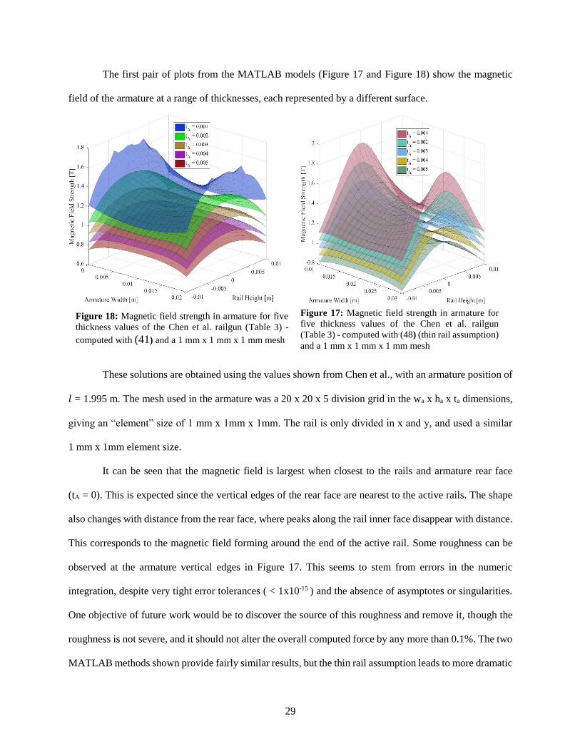
The first pair of plots from the MATLAB models (Figure 17 and Figure 18) show the magnetic
field of the armature at a range of thicknesses each represented by a different surface
These solutions are obtained using the values shown from Chen et al with an armature position of
119897 = 1995 m The mesh used in the armature was a 20 x 20 x 5 division grid in the wa x ha x ta dimensions
giving an ldquoelementrdquo size of 1 mm x 1mm x 1mm The rail is only divided in x and y and used a similar
1 mm x 1mm element size
It can be seen that the magnetic field is largest when closest to the rails and armature rear face
(tA = 0) This is expected since the vertical edges of the rear face are nearest to the active rails The shape
also changes with distance from the rear face where peaks along the rail inner face disappear with distance
This corresponds to the magnetic field forming around the end of the active rail Some roughness can be
observed at the armature vertical edges in Figure 17 This seems to stem from errors in the numeric
integration despite very tight error tolerances ( lt 1x10-15 ) and the absence of asymptotes or singularities
One objective of future work would be to discover the source of this roughness and remove it though the
roughness is not severe and it should not alter the overall computed force by any more than 01 The two
MATLAB methods shown provide fairly similar results but the thin rail assumption leads to more dramatic
Figure 18 Magnetic field strength in armature for five
thickness values of the Chen et al railgun (Table 3) -
computed with (41) and a 1 mm x 1 mm x 1 mm mesh
Figure 17 Magnetic field strength in armature for
five thickness values of the Chen et al railgun
(Table 3) - computed with (48) (thin rail assumption)
and a 1 mm x 1 mm x 1 mm mesh
30
peaks since all the current is concentrated along a line This means the thin rail model gives a maximum
that is 1176 larger (in this case) than the thick rail model though the average 119861 field value is only 465
larger (11843 T in the thin rail model 11317 T in the thick rail model) Another difference between the
two is the shape of the falloff with distance from the armature rear face The thin rail model falls off more
slowly and retains the peaks at the armature edges For example the bottom left corner of the two surface
plots shows that the thick rail model drops over 04 T between the largest and smallest thickness values
The same point in the thin rail model drops less than 03 T
These differences can also be seen in Figure 19 where the thick rail model drops to the minimum
value earlier than the thin rail model Regardless since the result of the two models is similar overall and
the thin rail model is computationally much quicker both models are carried forward
Mag
net
ic F
ield
Str
en
gth
[T
]
( a ) ( b )
Figure 19 Magnetic field strength in armature for the Chen et al railgun (Table 3) oriented as shown in Figure 20
( a ) - Thin Rail Model ( b ) - Thick Rail Model (both computed with a 04 mm x 04 mm x 01 mm mesh)
Figure 20 Orientation of Figure 19 armature magnetic field plots
Armature ldquoRear Facerdquo
31
The FEMM setup and results for the Chen et al
railgun comparison are shown in Figure 22 and Figure 21
The simulation considered the rails to be copper and the
armature to be Aluminum 6061-T6 The rails and armature
are surrounded by a region of air 0109 m in diameter with
a 119861 = 0 boundary applied around its circumference The
excitation current is applied to each rail separately so the
right rail receives an input of 140 kA and the left rail
produces an outlet current of -140 kA The elements are
planar first-order triangular elements with edges about
00014 m long (Meeker 2015) This result validates the shape of the 119861 field between the rails shown in
Figure 17 Figure 18 and Figure 19 where the field is largest at the center of the rail inner face and falls
off with distance from this point It also shows a more gradual falloff like that shown by the thick rail model
giving some justification for the extra computational time However the values produced by the MATLAB
models are approximately frac12 the magnitude of the FEMM results This discrepancy is explored more in the
next comparison
Figure 21 Comparison of MATLAB models
vs FEMM results along the armature centerline
(shown in Figure 22) for the Chen et al railgun
(Table 3)
119861 =
Figure 22 FEMM setup (a) and results (b) for the Chen et al railgun (Table 3) mesh 4704 Nodes 9046
Elements
Armature
Rail
y x Current
Outlet
Current
Inlet
( a ) ( b )
32
Though it is generally assumed here that current distribution in the rails is uniform a comparison
was done to look at the differences in magnetic field between uniformly distributed (laminated) rails and
solid rails This was done using a method demonstrated by Lv et al (2014) which uses a hollow rail to force
a static finite element solver to consider skin effects Since a negligible amount of current flows through
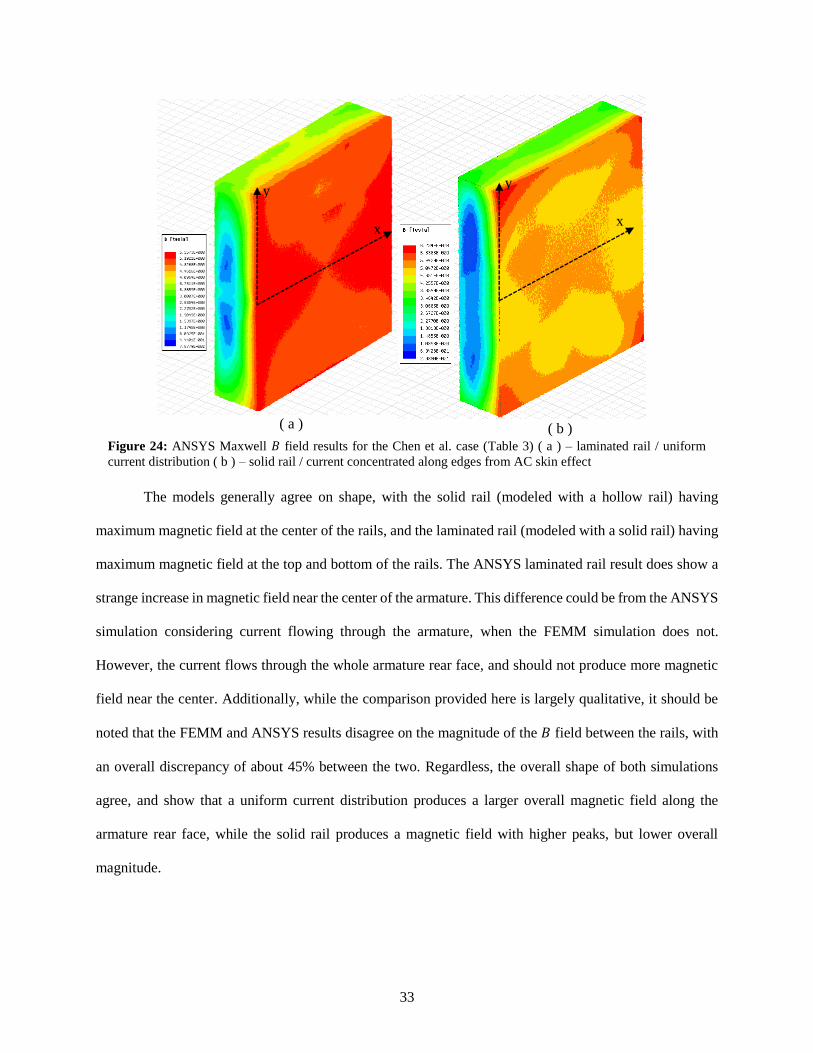
the center of solid rails this conductor material can be removed in the simulation Figure 23 and Figure 24
show the 119861 field in the armature as computed by FEMM and ANSYS Maxwell respectively
Table 4 Comparison of ANSYS and FEMM results for the Chen et al case
119861 Field [T]
Max Min
Solid Rail
FEMM 362286 26184
ANSYS 55573 481
Error -3481 -4556
Hollow Rail
FEMM 351901 260614
ANSYS 62344 485
Error -4355 -4627
Figure 23 FEMM 119861 field results for the Chen et al case (Table 3) ( a ) ndash laminated rail uniform current
distribution ( b ) ndash solid rail current concentrated along edges from AC skin effect
33
The models generally agree on shape with the solid rail (modeled with a hollow rail) having
maximum magnetic field at the center of the rails and the laminated rail (modeled with a solid rail) having
maximum magnetic field at the top and bottom of the rails The ANSYS laminated rail result does show a
strange increase in magnetic field near the center of the armature This difference could be from the ANSYS
simulation considering current flowing through the armature when the FEMM simulation does not
However the current flows through the whole armature rear face and should not produce more magnetic
field near the center Additionally while the comparison provided here is largely qualitative it should be
noted that the FEMM and ANSYS results disagree on the magnitude of the 119861 field between the rails with
an overall discrepancy of about 45 between the two Regardless the overall shape of both simulations
agree and show that a uniform current distribution produces a larger overall magnetic field along the
armature rear face while the solid rail produces a magnetic field with higher peaks but lower overall
magnitude
Figure 24 ANSYS Maxwell 119861 field results for the Chen et al case (Table 3) ( a ) ndash laminated rail uniform
current distribution ( b ) ndash solid rail current concentrated along edges from AC skin effect
( a ) ( b )
y
x
y
x
34
42 Comparison to Waindok and Piekielny
Table 5 Railgun parameters used throughout this paper used by Waindok and Piekielny (2016) (CC1)
The MATLAB and FEMM results for the Waindok and Piekielny comparison look very similar to
those of the previous comparison so plots resembling Figure 17 Figure 18 and Figure 23 are not presented
here As can be seen in Table 6 the magnitude of the 119861 field in the base Waindok and Piekielny railgun is
a little more than frac14 of that in the previous case While this case is about frac12 the size of the previous one
geometrically (which would suggest it should have a stronger magnetic field) it uses only 1 7frasl of the
excitation current so the smaller 119861 field is consistent with expectations The same 20 x 20 x 5 division is
used in this case meaning the element size is now 06 mm x 05 mm x 592 mm
Thick Model Error Thin Model Error
Average 119861 Field on Armature Centerline
Thick Model Thin Model FEMM
x01 20kA -499 -481 3926 4077 7833
x025 20kA -506 -488 1571 1631 3177
x05 20kA -518 -500 0785 0815 1628
x075 20kA -533 -516 0524 0544 1120
x1 1kA -552 -536 0020 0020 0044
x1 10kA -552 -536 0196 0204 0438
x1 20kA -552 -536 0393 0408 0877
x1 50kA -552 -536 0982 1019 2192
x1 100kA -552 -536 1963 2039 4383
x2 20kA -559 -543 0196 0204 0445
x5 20kA -556 -517 0079 0082 0177
x10 20kA -515 -498 0039 0041 0081 Table 6 Comparison of MATLAB models vs FEMM for the Waindok and Piekielny railgun (Table 5) ndash errors
computed by finding the error between the at each data point and averaging over the ndash uses a mesh with elements of
06 mm x 05 mm x 592 mm
Physical Parameters Symbol Value Value Symbol Electrical Parameters
Rail Length [m] L 02 1rarr20 IP Peak Current [kA]
Rail Separation [m] s 0012 ~ t1 Current Profile Rise Time [ms]
Rail Width [m] w 001 ~ t2 Current Profile Decline Time [ms]
Rail Height [m] h 001 ~ t3 Current Profile Total Time [ms]
Inductance Gradient [microHm] 119871prime 050 Value Symbol Material Parameters
Armature Width [m] wa 0012 Cu ~ Rail Material [~]
Armature Height [m] ha 00058 Al ~ Armature Material [~]
Armature Thickness [m] ta 00296 4 E -8 ρ Armature Resistivity [Ωm]
Armature Mass [kg] m 00056
Initial Velocity [ms] V0 0
35
The factor of ~2 discrepancy between the MATLAB models and finite element solutions also exists
in this comparison To further investigate this the change in 119861 field with a range of geometric scales and
excitation currents is examined to see how consistent this difference is The geometric scaling is done by
simply increasing each geometric value listed in Table 5 by a specified factor Thus the rails in the x2 case
are 2 cm x 2 cm rather than 1 cm x 1 cm
To perform this examination the 119861 field along the centerline of the armature (shown in Figure 21)
is plotted for both MATLAB methods and the FEMM results on the next page (Figure 25) The errors for
each method relative to the FEMM results are listed in Table 6 and show both MATLAB models to be
reliably about frac12 of the FEMM value The source of this consistent error is unknown and future work would
focus on this Ignoring the 119911 component of the 119861 field should not impact this as the 119861 field is only vertical
along the center of the rail face Assuming the current that flows the armature does not contribute to the 119861
field should not be responsible for this error since the FEMM simulation also does not consider current
flow in the armature Furthermore the ANSYS simulation (which does model current in the armature) gets
results similar to the FEMM model (a difference of 98 between maximum values) so this assumption
would not be responsible for a 50 error It should be noted that while the FEMM and ANSYS results for
the Chen et al case disagreed significantly their results for this case were consistently within 10
In addition to geometric scaling (which uses the 20 x 20 x 5 division scheme for each model) the
impact of mesh refinement was examined by reducing the element size to 006 mm x 005 mm x 0296 mm
for the 20 kA original geometry case This result had no discernable difference from the larger element size
for either the thick or thin rail case so it is unlikely that mesh size plays a significant role in model accuracy
36
Figure 25 Comparison of MATLAB models vs FEMM results for varying scales with the Waindok and
Piekielny railgun case (Table 5)
37
Lastly different rail aspect ratios were examined by changing the Waindok and Piekielny railgun
to use rails that are 2 cm wide by 1 cm tall and 1 cm wide by 2 cm tall When compared to FEMM results
the thick rail model maintained this factor of ~ frac12 relationship The thin rail model also maintained this
relationship for the 2 cm x 1 cm rail but the 1 cm x 2 cm rail exacerbates the peak-shape of the thin rail
model since there is more room for the field to fall off above and below the ldquowirerdquo that represents the rail
This means that the field is predicted to be larger than the thick rail model and departs from frac12 of the FEMM
result (the thin rail model predicts a maximum of 0512 T vs the thick rail result of 0329 T vs the FEMM
result of 0697 T) But the peak-like nature of this model means that the 119861 field at the top and bottom of the
armature is significantly underpredicted so the average value along the armature rear face is 030 T for the
thin rail model compared to 0279 T for the thick rail model It is predicted that these issues will be worse
for lower 119908 ℎfrasl ratio rails and railguns with wider armatures more rail separation However since this error
is consistent for the thick rail model and still fairly consistent for the thin rail model a correction factor of
2 is applied to the 119861 field equations of (41) and (48) to correct the MATLAB results to match those from
finite element solutions Even though the discrepancy is not exactly double and it is unlikely that a direct
factor of two is missing the application of this factor reduces the average error for all the cases in Table 6
from -529 to -58 This improved accuracy lends greater credence to the final force model which
depends on these methods
Also of note is that error for the thin
rail model decreases significantly near the
armature edges (rail faces) as shown in Figure
26 This corresponds to the more dramatic
peaks seen at the rail faces in the thin rail
model While the error is decreasing it does
not seem to be due to an actual increase in
accuracy Instead the erroneous peak in the
thin rail model partially cancels out the larger
Percent of distance across armature ( X direction )
Figure 26 Comparison of thick and thin rail model errors vs
FEMM for the x01 scale Waindok and Piekielny railgun case
(Table 5)
38
factor of ~ frac12 Since the thick rail model does replicate the shape of the FEMM results more accurately it
should still be seen as the more accurate model despite the fact that the thin rail model has lower average
error values
The shape of the thick rail model seems to be validated in the 119909ndash119910 plane by comparing the
MATLAB and FEMM results in Figure 19 and Figure 21 and the MATLAB and FEM results in Figure
27 and Figure 28 The shape in the 119911 direction can only be assessed by examining the ANSYS Maxwell
result The rate at which the 119861 field falls off with distance from the armature rear face is nearly equal
between the MATLAB and FEM results when accounting for the magnitude difference between the two
However the convex shape (as seen from the armature rear face) of the decreasing field shown in Figure
28 is not replicated by the MATLAB models The exact cause of this discrepancy is not known but it
should have little impact on the computed force as the current flowing through the front of the armature is
quite small and the 119861 field drops to levels that are similarly small between the MATLAB and FEM results
This chapter has presented two methods to compute the magnetic field in the armature and
compared them to finite element solutions in FEMM and ANSYS Maxwell Overall once the correction
factor has been introduced both of these methods agree well with finite element results and lend themselves
to use in computing force in MATLAB and similar software packages While the thick rail model is more
accurate than the thin rail model it is yet to be seen if the extra computational effort required for the thick
rail model is justified This will be determined in the force computation chapter
39
Mag
net
ic F
ield
Str
ength
[T
]
(a) (b)
Figure 27 Magnetic field strength in armature for the Waindok and Piekielny railgun (Table 5)
orientation shown in Figure 20 ( a ) - Thin Rail Model ( b ) - Thick Rail Model
Figure 28 ANSYS Maxwell result for the Waindok and Piekielny railgun (Table 5) The origin has been
shifted to stay on the armature rear face in this figure for readability but all computations are done considering
119911 = 0 to be at the breech
y
x
z
40
Chapter 5 Inductance Gradient
Many equations describing railgun operation such as those for current distribution force and
efficiency can be greatly simplified using the inductance gradient (119871prime) (Bayati et al 2011) (Murugan et al
2016) (McCorkle and Bahder 2010) 119871prime is measured in microhenries per meter (microHm) and is a function of
rail geometry rail separation (s) rail material and current distribution as a function of time (Keshtkar 2005)
(Keshtkar et al 2009) (Huerta and Nearing 1991) Since railguns operate on DC current dependence on
transient current distribution is normally neglected (Keshtkar et al 2009) though the skin effect (which is
due to transience as described in the current distribution section) is frequently considered Thus for the
simple case of a railgun with rectangular copper rails 119871prime is considered to be dependent only on rail
separation (s) rail width (w) and rail height (h) as shown in Figure 29
Usually it is necessary for researchers to use a finite element or finite
difference approach to compute 119871prime While this is more accurate it is time
consuming and pushes railgun designers to depend on tables like the ones
provided by Keshtkar et al (2009) and others For convenience a compilation of
the tables located during this investigation is provided in Appendix A Due to the
effort required to calculate 119871prime via FEA multiple approximation methods have
been developed using only geometric values This simplicity comes at a cost though as it generally limits
the application of these methods to rectangular rails (as shown in Figure 29) The derivation of many of
these approximation methods rely on the fact that in railguns with solid rails significant current only flows
through a thin layer on the rail surface The depth of the current distribution is called ldquoskin depthrdquo (Keshtkar
2005) (Huerta and Nearing 1989) (Keshtkar Bayati and Keshtkar 2009)
h
w
s
y
x
Figure 29 Dimension
description for
rectangular rails
41
51 Kerrisk Method
A common approach called the Kerrisk method was developed for rectangular conductors by J F
Kerrisk in 1981 at the Los Alamos National Laboratory (Kerrisk 1982) (Jin et al 2012) In developing this
method Crandallrsquos method was used to compute the current distribution in the rails The inductance and
magnetic flux of the circuit were then found
eventually leading to 119871prime by integrating the magnetic
field strength over the conductor area This process
yielded (51) and values shown in Table 7 were
found by performing a least squares fit of this
equation to the obtained 119871prime results
(49) 1198651 = 1 + 1198701198861times(119908
ℎ) + 1198701198862times
119908
ℎtimes119904
ℎ
(50) 1198652 = 1198701198871 + 1198701198872times119904
ℎ+ 1198701198873times
119908
ℎ+ 1198701198874times
119904
ℎtimes119908
ℎ
(51) 119871prime = [ 119860 + 119861times ln(1198651) ]timesln (1198652)
This finally produces a relatively easy-to-use equation (52) (Kerrisk 1982)
(52) 119871prime = [119860 + 119861times ln (1 + 1198701198861times(119908
ℎ) + 1198701198862times
119908
ℎtimes119904
ℎ)]hellip
hellip timesln (1198701198871 + 1198701198872times119904
ℎ+ 1198701198873times
119908
ℎ+ 1198701198874times
119904
ℎtimes119908
ℎ)
In this process the following assumptions were made
The conductors (rails) are very long in the z direction (into the page in Figure 29)
Current only flows in the z direction
Current only flows on the conductor surface
The conductor corners are rounded (current density would become infinite for square corners)
The circuit is symmetric about the x-axis
Value Standard Deviation
A [microHm] 04406410 00032
B [microHm] -00777133 00014
Ka1 3397143 0146
Ka2 -00660307 00069
Kb1 1007719 00089
Kb2 2743651 00581
Kb3 00220931 00036
Kb4 02637392 00368
Table 7 Kerrisk method coefficients
42
This equation was implemented and a replication of Kerriskrsquos results showing very good
agreement is shown in Figure 56 Figure 57 and Figure 58 of Appendix B These were made by
superimposing Kerriskrsquos results on the MATLAB results computed here
52 Huerta Conformal Mapping Method
Another approximation method was developed for rectangular rails by Huerta et al in 1991 To
develop this method conformal mapping and the Schwartz-Christoffel transformation were used to map
the rail boundaries In doing this Huerta et al assumed the following
The rail dimensions are much larger than the skin depth
The current travels only on the rail surface
There is no magnetic field inside the rails
It is interesting to note that the singularity presented by sharp corners is not an issue here as this method
does not require a numeric computation of current distribution The equations used to find 119871prime with this
method are provided as Equations (53) rarr (56) including the complete elliptic integral (119870) (Gradshteyn
and Ryzhik 2007)
(53) 119871prime = 1205830times119870(119896prime)
119870(119896)
(54) 119896prime = radic119906119873 = radic1 minus 1198962
(55) 119896 = radic1 minus 119906119873
(56) 119870 = 119888119900119898119901119897119890119905119890 119890119897119897119894119901119905119894119888 119894119899119905119890119892119903119886119897 = 119870(119896) = int1
radic1minus1198962lowastsin (119909)2 119889119909
1205872frasl
0
This approach is less simple than others and requires that Equations (57) rarr (61) on the next page
be root-solved for the unknowns 119906119873 119906119874 and 119906119875 A table of solved values from this method can be found
in Figure 52 of Appendix A Inductance Gradient Tables (Huerta and Nearing 1991)
43
(57) 119866(119886 119887 119888 119889 119890) = int |(119906minus119888)lowast(119906minus119889)
119906lowast(119906minus119890)lowast(1minus119906)|12frasl
119889119906
119887
119886
(58) 119904
2= 120572times119866(0 119906119873 119906119874 119906119875 119906119873)
(59) ℎ
2= 120572times119866(119906119873 119906119874 119906119874 119906119875 119906119873)
(60) ℎ
2= 120572times119866(119906119875 1 119906119874 119906119875 119906119873)
(61) 119908 = 120572times119866(119906119874 119906119875 119906119874 119906119875 119906119873)
53 Intelligent Estimation Method (IEM)
In 2009 Keshtkar Bayati and Keshtkar developed an equation for the 119871prime of rectangular rails using
the Intelligent Estimation Method (IEM) IEM consists of the compilation of significant variables a
breakdown into analytically known physical components a linear combination of these components using
weighting coefficients and finally a comparison to experimental results If the error is not negligibly small
the weighting coefficients are recalculated and this process is repeated until errors become small In
applying this to the computation of 119871prime Keshtkar et al assumed that
Current only flows on the outer surface of rectangular conductors
These outer faces can be separated into 4 distinct pairs of plates (one pair being the top surface of
each rail the second being the right surface of each rail and so on)
The current that flows into one plate on the first rail flows out of the corresponding plate on the
second rail
Using these assumptions and the IEM Keshtkar Bayati and Keshtkar found the 119871prime of each pair of plates
These were then linearly combined as shown in (62)
(62) 1
119871prime= 1198601times
ℎ
119904+ 1198602times
ℎ
119904+2times119908+ 1198603times
1
119897119899(4times(119904+119908)
119908)+ 1198604times
1
119897119899(4times(119904+119908)
119908)
44
The coefficients were computed by comparing initial values to FEA results and correcting until
the error became sufficiently small The resulting 119871prime equation is shown as (63) This method will be referred
to as the IEM method in the rest of this paper (Keshtkar Bayati and Keshtkar 2009)
(63) 119871prime = 10minus6
05986timesh
119904 + 09683times
h
(s+2timesw) + 43157times
1
ln(4times(s+w)119908
) minus 07831
Similar to the Kerrisk method description this method was implemented and a replication of the
results produced by Keshtkar et al showing very good agreement is shown in Figure 59 Figure 60 and
Figure 61 of Appendix B These were again made by superimposing the results of Keshtkar Bayati and
Keshtkar on the MATLAB results computed here
54 119923prime Regression Method (LRM)
The most recent approximation method was developed by Murugan et al and was published in 2016 This
method uses regression analysis with the Oakdale Data Fit Engineering software program to approximate
119871prime from FEM results obtained using ANSOFT The software program computes 254 equations to describe
119871prime and the best of these were chosen with regression values Ra rarr Rj provided in Table 8 LRM regression
values This method will be referred to as the Inductance Gradient Regression Method (LRM) in this report
Rectangular Circular (θ=40ordm) Circular (θ=10ordm)
Ra 045173 028119 011373491
Rb 025006 -0088383 -003997613
Rc -006491813 0540073 013263606
Rd 004216090 000476755 0016023852
Re -000454295 -19731854 -029597112
Rf -003898298 -0048983 -0062019418
Rg 0000974821891 00028816 000425462548
Rh 00018307804 2780857 039459707
Ri -000416014722 -0012536 00337784518
Rj -000581360388 -00199827 -000645150442 Table 8 LRM regression values
45
Unlike the other methods listed this approximation also considers circular rails However
analytical limitations arise because the geometry of circular rails is described by two units (length and
angle) instead of one (length) The geometry of this sort of rail is shown as Figure 30
and can be described by thickness (t) separation (s) and opening angle (θ) This means
that instead of one equation that can be used for all geometric configurations circular
rails require one value to be held constant Murugan et al decided to hold opening angle
constant and compute equations for rails with θ values of 10 and 40 degrees These
both use (65) but use different regression values from Table 8 (Murugan et al 2016)
(64) 119871prime119903119890119888119905119886119899119892119906119897119886119903 = 119877119886 + 119877119887 times ln (119904
ℎ) + 119877119888 times ln (
119908
ℎ) + 119877119889 times ln (
119904
ℎ)2
hellip
hellip+ 119877119890 times ln (119908
ℎ)2+ 119877119891 times ln (
119904
ℎ)times ln (
119908
ℎ) hellip
hellip+119877119892times ln (119904
ℎ)3+ 119877ℎ times ln (
119908
ℎ)3
hellip
hellip+ 119877119894 ln (119904
ℎ)times ln (
119908
ℎ)2+ 119877119895 times ln (
119904
ℎ)2times ln (
119908
ℎ)
(65) 119871prime119888119894119903119888119906119897119886119903 = 119877119886 + 119877119887 times 119897n (119905
119904) + 119877119888times(
1
119904) + 119877119889 times ln (
119905
119904)2+ 119877119890 times (
1
119904)2
hellip
hellip+119877119891 timesln(119905
119904)
119904+ 119877119892 times ln (
119905
119904)3+ 119877ℎ times (
1
119904)3+ 119877119894 times (
ln(119905
119904)
119904)
2
hellip
hellip+119877119895 times (ln(119905
119904)2
119904)
55 Comparison of 119923prime Methods
Inductance gradient values have been found using the Kerrisk IEM and LRM methods and a comparison
has been performed Previous investigations (Kerrisk 1982) (Murugan et al 2016) have compared the
results from these methods to finite element or finite difference results using various separation-to-height
and width-to-height ratio values One method uses the following four cases to compare results for
rectangular rails
s y
x
t
θ
Figure 30 Dimension
description for
circular rails
46
Case 1 high 119904
ℎ and high
119908
ℎ Case 2 low
119904
ℎ and low
119908
ℎ
Case 3 high 119904
ℎ and low
119908
ℎ Case 4 low
119904
ℎ and high
119908
ℎ
The results of this comparison can be seen in Figure 31 These plots show reasonable agreement between
the methods with the exception of the IEM in Case 3 which departs significantly from the other methods
The IEM is generally the outlier in this comparison and is the least accurate when compared to FEM results
in Case 2 The FEM values used here come from the article by Murugan et al in which the LRM is
introduced (Murugan et al 2016) FEM values were not available for comparison in the other cases
Because Murugan et al present FEM results over the range of sh and wh from 01 to 1 a surface
plot is presented in Figure 32 on the next page This shows a similar agreement between the methods with
the IEM showing the most disagreement The error of each method is plotted in Figure 33 and quantified
in Table 9 also on the next page The LRM has the smallest error but this does not necessarily mean it is
the most accurate as it was developed using the FEM values used here
(a)
(c) (d)
(b)
Figure 31 4-Case Comparison of 119871prime Computation Methods
47
LRM IEM Kerrisk Method
Average Error 0276 3068 0718
Table 9 119871prime analytical method errors vs FEM (Murugan et al 2016)
Figure 32 Comparison of 119871prime methods to FEM (Murugan et al 2016)
[microH
m]
Figure 33 119871prime analytical method error vs FEM (Murugan et al 2016)
48
A look at a broader range of sh and wh ratios is shown in Figure 34 and Figure 35 This shows some
disagreement between the models mainly at large sh and low wh where the LRM gives a result of 159
microHm the Kerrisk method gives 141 microHm and IEM gives 110 microHm
Overall the IEM agrees well with both finite difference and LRM results when sh and wh are
both high or both low But when sh is high and wh is low or when sh is low and wh is high there is
significant disagreement between IEM and other methods For these cases both LRM and the Kerrisk
method agree well with finite element methods
No other analytic method of computing 119871prime for circular rails was found so no comparison to other
estimation methods is presented though Murugan et al do compare their results to their own FEM values
Other sources of 119871prime values computed with FEM techniques were almost as scarce In fact only one data
point was found (Bayati et al 2012) which could be compared to (65) There do exist tabulated 119871prime values
10 9
Figure 34 Broad comparison of 119871prime methods
[microH
m]
Figure 35 Broad comparison of 119871prime methods
[microH
m]
49
computed with FEM (shown in Figure 55 of Appendix B) but none could be found which used an opening
angle of 10 or 40 degrees besides the values that the LRM equation was developed from Thus because
simulating 119871prime is outside of the scope of this investigation no assessment of accuracy is provided here
Regardless (65) represents an easy-to-use method of computing 119871prime values without the need for a finite
element model This method has been compared to FEM values by its creators and a very similar method
was used to define the LRM for rectangular rails
The obvious shortcoming of all these methods is that they are only valid for predetermined
geometries and while this is better than relying on tabulated values designers interested in more complex
geometries or more nuanced railgun methods will need to run their own simulations to compute 119871prime
This chapter presents four different methods of computing 119871prime which have already been defined in
readily applicable forms Three of these methods are replicated (the Kerrisk method IEM and LRM) and
compared to each other and finite element values It has been determined that two of these methods (the
Kerrisk method and the LRM) are more accurate than the other Thus when 119871prime is calculated throughout this
paper it is done by averaging the Kerrisk and LRM results for a given geometry
50
Chapter 6 Force Computation
The fundamental force behind railguns and the main focus of this investigation is the Lorentz
force It is suggested here that a method which computes force by directly approximating current
distribution and magnetic field in the armature can provide more accurate force values than the traditional
railgun force equation while being more readily applicable than finite element computations This
hypothesis is tested by comparing the railgun force equation to five other approximations of railgun force
with three finite element solutions from the literature one set of experimental values from the literature
and one finite element solution defined here A mesh refinement of this mid-complexity model is also
presented Regardless of which solution is more accurate this review also inherently presents a brief look
at the consistency of railgun force modeling
The Lorentz force is generated by charge moving through a magnetic field and its equation is
shown here as (66) As is the case for all railgun parameters the complete solution of (66) requires the
computation of simultaneous partial differential equations to compute the current distribution (119921) and
magnetic field (119913)
(66) 119865 = ∭ 119921 times119913 119941119933119881
Approximations have been made by Waindok and Piekielny (2016) in equations (67) and (68) and
Xu and Geng (2010) in equation (70) on the following page which use the Biot-Savart law to compute
magnetic field The traditional railgun force equation is presented in (71)
(67) 119865 = int 119868(119905) ∙ 119861 1198891199091199081198600
= int μ0 ∙ I(t)
2
4 ∙ π ∙ x ∙ (
119897
radic119897 2+ 1199092) 119889119909
119908119860
0
(68) 119865 = μ0 ∙ I(t)
2
4 ∙ π ∙ (minus 2 ∙ 119897119899 (
119897+radic119897 2+ 1198892
119889) + 119897119899 (
119897+radic119897 2+ 119908
4
2
119908
2
)+ 119897119899 (119897+radic119897
2+ 1199081198602
119908119860))
119908ℎ119890119903119890 119889 = 119908119860 +119908
2
(69) 119866 = 2 ∙ (x+119909prime)
(yminusyprime)2+(x+xprime)2 ∙ [
z
radic(yminusyprime)2+(x+xprime)2+1199112minus
zminusl
radic(yminusyprime)2+(x+xprime)2+(zminusl)2]
51
(70) F =μ0
2 ∙ π ∙ h2 ∙ w ∙ t119886
int
int int (int int 119866 ∙ I(x y z t)2 h
2
minush
2
w
0
dyprime ∙ dxprime)
119908119860
0
h1198602
minush1198602
119897+119905119860
119897
∙ 119889119909 ∙ 119889119910 ∙ 119889119911
(71) F =119871prime ∙ 119868(119905)2
2
These approximations make the following assumptions
The current is distributed uniformly in the rails
o This is a significant approximation for solid rails as the 119861 field between the rails
is higher but becomes reasonably accurate for laminated rails (Xu and Geng 2010)
(Xing et al 2015)
Force is only produced by the 119913119962 component of the magnetic field
o This assumption is reasonably accurate since the dominant component of the
magnetic field between the rails points in the y direction (shown in Figure 36)
though the Bx component is visibly non-zero near the top and bottom of the bore
Figure 36 Magnetic field around rails as computed by ANSYS Maxwell 172
y
x
52
The current moves perpendicular to the rail inner face at all points in the armature (similar
to Figure 1 and Figure 9)
o This assumption is fairly accurate for rectangular armatures (which is the only
geometry modeled here) but falls apart for ldquoC shapedrdquo armatures (shown in Figure
38 and Figure 41) Even in rectangular armatures the current does not turn
instantly as shown by Figure 37
The complexity of (66) rarr (70) comes from defining the magnetic field in the armature and
accounting for the discretization of the armature and rail Further explanation of the equations for magnetic
field is presented in the magnetic field section It should be restated that as described in the magnetic field
section a factor of 2 was added to the magnetic field calculation to better match the 119861 field with finite
element results This is shown in (70) where the denominator of the leading coefficient contains a factor
of 2 rather than a factor of 4 as shown in (41) Further approximations have been made to produce the
widely used and very simple ldquorailgun force equationrdquo (71) by utilizing the induction gradient (119871prime) (Coffo
2011) (Behrens et al 2003) (Ya-Dong et al 2012) (Keshtkar 2005) (Keshtkar et al 2009) (Murugan et al
2016) (Keshtkar 2005) (Moghaddam et al 2004) (Xu et al 2014) (Schneider et al 2009 pt1) (Schneider et
al 2009 pt2) (McCorkle and Bahder 2010) (He et al 2010) (Chen et al 2015) All of the methods presented
here neglect aerodynamic drag
Figure 37 Current flow in rails and armature as computed by ANSYS Maxwell 172
z
x
53
The time dependent current is computed by (1) rarr (4) in the power supply section and assumes
that most railgun current profiles can be approximated by a sinusoidal rise a constant maximum and an
exponential decay
The frictional force used here is shown in (72) and relies on an approximate sliding friction
coefficient computed experimentally by Chen et al of 120583119891 = 011 (Chen et al 2014) (Chen et al 2015)
(72) 119865119891 = 120583119891 ∙ 119865119888 = 011 ∙ ( 001 ∙ 119868 ) = 00011 ∙ 119868
Obviously in application this coefficient is dependent on the specific materials surface smoothness
and surface treatments or lubricant used The normal force is computed by assuming the ldquogram per amprdquo
rule is followed as is done by Jin et al (Jin et al 2012) This rule developed by Richard Marshall specifies
that one gram of mechanical preload (normal force from the armature on the rail) should be applied per
amp of excitation current to maintain good electrical contact throughout launch though this remains an area
of active research (Brady 2005) (Chen et al 2014) In the fourth comparison case considered below a
different formulation for 119865119862 presented by Chen et al (2015) is used (73)
(73) 119865119862 = 119871prime ∙ 1198682 ∙ 119889 ∙ 120579119888119886
119908119886
This formulation is developed for a very specific armature shape (Figure 38) so it is not generally
applicable though it could be used to approximate 119865119862 for C-shaped armatures This would only be an
approximation because most C armatures contact the rail along the whole length of the ldquolegsrdquo while the
special armature considered below only contact the rail at the very end of the legs
These force equations were solved and numerically integrated using an RK4 integration scheme in
MATLAB In this integration the initial position of the armature must be set to some positive value to
avoid numeric issues at 119897 = 0 As stated before the double integral over the rail cross-section (inside the
parentheses in (70)) is computed using the ldquointegral2rdquo MATLAB function The integral over the armature
volume (outside the parentheses in (70)) is computed with the ldquotrapzrdquo MATLAB function
54
Six different solution methods examined in this chapter and are described in Table 10 These
models have been compared to experimental results and other models from the literature including finite
element solutions
Each comparison consists of a description of the initial method and findings a description of the
values used to attempt to replicate the results a display of the results and a discussion of the comparison
The first comparison (CC1) also includes ANSYS results made in this investigation and a rudimentary mesh
refinement study of the F3 and F4 methods The properties of each compared railgun will be presented in
a table Some of these comparisons required assumptions and these are highlighted in grey The inductance
gradient in these tables has been computed by averaging the Kerrisk and LRM methods this and other
computed values are highlighted in yellow Frictional effects are only considered when comparing to
Method Symbol Description
Railgun Force S1 Classical railgun force equation (71)
Waindok and Piekielny Force S2 Direct force equation defined by Waindok and Piekielny (68)
Uniform Current Thick Rail F1
Magnetic field computed in armature with thick rail method
and multiplied by current density at each point Current
density is assumed uniform
Uniform Current Thin Rail F2
Magnetic field computed in armature with thin rail method
and multiplied by current density at each point Current
density is assumed uniform
Non-Uniform Current Thick
Rail F3
Magnetic field computed in armature with thick rail method
and multiplied by current density at each point Current
density in armature takes skin effects into consideration
Current density in rail assumed uniform
Non-Uniform Current Thin
Rail F4
Magnetic field computed in armature with thin rail method
and multiplied by current density at each point Current
density in armature takes AC skin effects into consideration
Current density in rail assumed uniform Table 10 Description of force computation methods
Figure 38 Special armature used by Chen et al to study melt wear rate (Chen et al 2015) ( a ) ( b )
55
experimental results or other models which consider friction as it is commonly neglected When
determining the current density in the armature the SAC is used to find the skin depth (δ) and the CStSM
is used to determine density (32)
61 Comparison Case 1 (CC1) Waindok and Piekielny (2016) and
ANSYS Maxwell Waindok and Piekielny compare railguns with and without iron cores and permanent magnets to
determine their improved efficacy Their research also defines an analytic equation for simple railgun force
(method S2) and compare this to a numerical solution obtained using ANSYS Maxwell Both of these
results for the three simple railgun cases presented by Waindok and Piekielny are compared to the models
used here (Table 10) The values used for this railgun are shown in Table 5 The source article does not
consider friction so it is also neglected in the comparison analysis The armature height had to be found by
using the given mass and assuming the armature is rectangular and made of aluminum (2700 119896119892
1198983) The
source material only shows the force on the armature for certain applied excitation currents Thus the
methods used here are only compared to these force values at specific currents and no time-histories are
presented Essentially three different comparisons are made here one between the methods developed here
and the results from Waindok and Piekielny one between these methods and an ANSYS Maxwell 172
model and one between these methods computed with various mesh sizes The results for the first two
comparisons are shown in Table 12 and mesh refinement results are shown in Table 13
Excitation Current [kA]
Force [N]
Analytic Equation
(Waindok and
Piekielny 2016)
ANSYS Maxwell
(Waindok and
Piekielny 2016)
20 11075 1306
10 277 3265
1 028 033
Table 11 Results produced by Waindok and Piekielny for CC1 (Table 5)
56
Geometric
Scale
Excitation
Current [kA]
Force [N]
S1 S2 F1 F2 F3 F4 ANSYS
x01 20 10004 97721 49567 52620 49003 52046 90281
x025 20 10004 97721 49567 52620 58663 62288 8977
x05 20 10004 97721 49567 52620 71788 76057 89755
x075 20 10004 97721 49567 52620 80254 84749 90981
x1 1 025 024 012 013 021 022 02249
x1 10 2501 2443 1239 1315 2128 2239 2244
x1 20 10004 9772 4957 5262 8512 8957 89953
x1 50 62527 61076 30979 32887 53202 55980 56221
x1 100 25011 24430 12392 13155 21281 22392 22488
x2 20 10004 97721 49567 52620 89904 93399 90694
x3 20 10004 97721 49567 52620 89265 92002 89436
x4 20 10004 97721 49567 52620 88455 90777 88286
x5 20 10004 97721 49567 52620 87963 90075 8523
x10 20 10004 97721 49567 52620 87465 89382 87479
Average
Error
vs Analytic -2370 -2590 -6260 -6000 -3530 -3210 -1915
vs ANSYS -1000 -1260 -5590 -5290 -2380 -1990 -3142
vs ANSYS 1194 921 -4466 -4117 -984 -587 ~
Table 12 CC1 Results found at 119897 = 01704 m with grid elements 06 mm x 05 mm x 296 mm large ( ha x wa x ta ) at
the x1 scale Green highlights are compared to the Waindok and Piekielny (2016) results
Geometric
Scale
Excitation
Current [kA]
Force [N] for different numbers of armature divisions ( wa x ha x ta )
40 x 40 x 20 60 x 60 x 30 80 x 80 x 40 ANSYS
F3 F4 F3 F4 F3 F4
x01 20 52268 55757 53516 57132 54170 57845 90281
x025 20 62698 66938 64311 68729 65168 69667 8977
x05 20 77808 83039 80360 85879 81743 87397 89755
x075 20 88595 94398 92321 98539 94378 100795 90981
x1 1 0239 0254 0251 0268 0258 0275 022488
x1 10 23890 25400 25120 26764 25813 27523 2244
x1 20 95561 101599 100481 107057 103253 110090 89953
x1 50 597254 634993 628007 669104 645330 688065 56221
x1 100 2389016 2539971 2512028 2676417 2581320 2752262 22488
x2 20 104426 109985 112964 119396 118203 125092 90694
x3 20 103418 108069 113661 119314 120513 126731 89436
x4 20 100669 104561 111312 116217 119065 124582 88286
x5 20 98000 101328 108265 112551 116392 121301 8523
x10 20 91363 93540 96951 99620 103364 106494 87479
Average
Error
vs Analytic -1405 -862 -962 -371 -713 -098 -1915
vs ANSYS -2709 -2248 -2333 -1832 -2122 -1600 -3142
vs ANSYS 053 600 688 1298 1116 1763 ~
Table 13 Mesh refinement assessment done at 119897 = 01704 m with grid element sizes varying from 03 mm x 025 mm
x 148 mm to 015 mm x 0125 mm x 074 mm Green highlights are compared to the Waindok and Piekielny (2016)
results
57
The comparison to the Waindok and Piekielny results was surprising since the model pulled from
this paper (S2) did not match up with their analytic results In the source article the FEM results show that
the armature force does not vary significantly (if at all) with armature position However it can be seen just
by inspection of (68) that changes in 119897 will impact the armature force with method S2 This may be
responsible for some of this variation since the armature position is not stated in the source material (using
119897 = 01704 depends on an assumption that the armature is about to leave the rails) But force increases with
armature position using method S2 and even with the armature at the rail end ( 119897 = 02 m ) the 20 kA force
would be 9790 N not 11075 N Regardless of the agreement between the two results it is concluded that
the significant position dependent variation in force suggested by this formulation is erroneous since the
ANSYS results from Waindok and Piekielny and the LS-DYNA results from Jin et al (in CC3 below)
show very little change with position It should be mentioned that this does not only occur in the S2
formulation In fact all of the methods presented here besides the simple railgun force equation (S1) show
some of this behavior mainly visible in Figure 43 ( b )
Another possible explanation of the disagreement could be that the armature and rail heights used
here are different than the original analysis However armature and rail height do not show up in the S2
force equation (68) so any incorrect assumption of these values should not impact this specific result Lastly
the ANSYS Maxwell 172 results calculated in this assessment match models S1-S4 much better than the
ANSYS Maxwell 140 results from the source article This further suggests some yet unconsidered
difference between the two models as one would expect the two finite element models to produce results
that have less than ~30 error
The quantitative results of this comparison are shown in the rows highlighted in green in Table 12
The average errors for S1rarrF4 are relative to the results shown in Table 11 and Table 12 and only use the
values corresponding to the cases shown in Table 11 (scale of x1 and excitation current of 20 10 and 1kA)
58
The ANSYS results referenced in Table 12 and Table 13 are computed using the model setup shown
in Figure 39 with the magnetostatic solver in ANSYS Maxwell 172 The current excitation is applied in a
way similar to the FEMM model in Figure 21 where an inlet and outlet current is specified at the rear face
of each rail A 119861 = 0 boundary is applied along the walls of a cylindrical region around the rails This region
is coincident with the rail rear and front faces The model uses an adaptive mesh of tetrahedral elements
with an average edge length of ~ 015 mm The values used in these tables are the 119865119910 force components
which are by far dominant over the other two (the 119865119909 components are ~ 02 of 119865119910 and the 119865119911 components
are ~ 002 of 119865119910 )
Models S1 S2 F3 and F4 show good agreement with the ANSYS Maxwell 172 results The F1
and F2 results significantly underestimate the force This makes sense because these cases do not consider
the high current density along the armature rear face meaning much of the current is considered to flow
through a region which has small 119861 field and thus creates less force than other methods It is worth noting
that the simple methods ( S1 and S2 ) perform similarly to the more complex ones ( F3 and F4 ) These
simpler methods do not change with geometric scale which is not inaccurate as the ANSYS results are
fairly constant with scale change as well The more complex models mirror this for larger scales but suffer
some issues with smaller geometries This could not be readily explained and is the reason a mesh
refinement study was done on these two models (Table 13) The F4 model despite relying on the thin rail
assumption has a smaller average error than the F3 model which uses the more accurate thick rail method
of finding 119861 It seems that this is due to a general underestimate by both methods and the thin rail model
Figure 39 Setup for the ANSYS Maxwell 172 Lorentz force model
59
happens to find larger overall values than the thick rail model This is not always the case as F4
overestimates the ANSYS results in the x2 to x10 scale models
This mesh refinement assessment reveals an alarming relationship between number of grid
elements and computed force where more grid elements (smaller grid element size) corresponds to higher
force For the size of elements considered here no leveling off of this effect can be seen (Figure 40)
Though the total amount of current (computed with (34)) remains equal to the excitation current
regardless of element size the average current density increases with the number of elements Some further
investigation showed the decrease in element size in the z direction to be responsible for most of this
increase with x direction size making up the rest of the increase This seems to suggest numeric issues
related to the concentration of current density points along the armature rear face though the exact
mechanism of this could not be determined Resolving this issue represents the most significant objective
of any future work The first steps in this would be to compare element size to the armature skin depth and
further reduce the mesh size As Figure 40 shows the error does seem to curve and may level off for even
smaller meshes It should be mentioned that run times get prohibitively long for F3 using such meshes The
run time for this analysis was 43 s and 024 s for F3 and F4 respectively with a grid element scale factor
of 1 and 291 s and 0290 s for F3 and F4 respectively with a scale factor of 0125 This demonstrates the
Figure 40 Method F3 and F4 error relative to the ANSYS Maxwell 172 results
for grid element sizes varying from 03 mm x 025 mm x 148 mm to 015 mm x
0125 mm x 074 mm
60
computational load that accompanies the ldquointegral2rdquo computation However if the worst case is true (that
the force result is simply arbitrary relative to the number of elements used) then it is unlikely that these
equations will produce reliably accurate results across multiple cases This provides further motivation for
the following force comparison cases
62 Comparison Case 2 (CC2) Chengxue et al (2014)
Physical Parameters Symbol Value Value Symbol Electrical Parameters
Rail Length [m] L 1 1rarr5 IP Peak Current [100000 A]
Rail Separation [m] s 002 05 t1 Current Profile Rise Time [ms]
Rail Width [m] w 0006 17 t2 Current Profile Decline Time [ms]
Rail Height [m] h 002 30 t3 Current Profile Total Time [ms]
Inductance Gradient [microHm] 119871prime 052 Value Symbol Material Parameters
Armature Width [m] wa 002 Cu ~ Rail Material [~]
Armature Height [m] ha 002 Al ~ Armature Material [~]
Armature Thickness [m] ta 001 4 E -8 ρ Armature Resistivity [Ωm]
Armature Mass [kg] m 02599
Initial Velocity [ms] V0 0
Table 14 Railgun parameters for comparison case 2 (CC2) (Chengxue et al 2014)
Chengxue et al also utilize ANSYS to perform a
FEM simulation of railgun armature force and heating While
a current profile is shown no mention of final velocity is
provided in this source material Railgun armature force is
instead provided for different excitation currents again so a
comparison similar to that of CC1 is provided here
Chengxue et al use a popular C armature geometry (shown
in Figure 41) which is not supported by the models used here
It is approximated by a rectangular armature which has its
edges delineated by the contact patch of the C armature with the rails The railgun properties used here are
shown in Table 14 The original article ignores the frictional force and so does this comparison The
armature mass was obtained using the volume of the C armature and the density of aluminum (2700 119896119892
1198983)
Figure 41 C armature illustration (Chengxue
et al 2014)
61
Results from this comparison are shown in Table 15 and favor the simpler S2 method
Excitation
Current [kA]
Force [kN]
ANSYS
(Chengxue
et al 2014)
S1 S2 F1 F2 F3 F4
500 1719 65016 101837 78977 86836 77703 85739
400 692 4161 65175 50545 55575 49731 54873
300 267 23406 36661 28432 31261 27973 30866
200 1262 10402 16294 12636 13894 12433 13718
100 712 2601 4074 3159 3473 3108 3429
Average Error -3909 -459 -2601 -1864 -2720 -1967
Table 15 CC2 Results computed at 119897 = 099 m with grid elements 1 mm x 1 mm x 05 mm in size
The other methods stay reasonably close but do underestimate force in this scenario Part of this
could be due to the C shaped armature which can obtain higher force than rectangular armatures by
extending the active magnetic space between the rails by taking advantage of the current flowing through
the armature ldquolegsrdquo A study by Bayati et al (2015) on the specifics of this C shape have determined that
longer legs produce more force at the cost of higher maximum current density (and thus more ohmic
heating)
The difference between considering uniform current distribution in the armature and not (F1 and
F2 vs F3 and F4) is much less significant in this comparison than CC1 The last comparison used a very
thick armature compared to this one meaning a uniform current distribution would pull much more current
away from the high 119861 field area of the armature Since this case uses a significantly thinner armature a
uniform distribution is less consequential
62
63 Comparison Case 3 (CC3) Jin et al (2015)
Physical Parameters Symbol Value Value Symbol Electrical Parameters
Rail Length [m] L 03 700 IP Peak Current [kA]
Rail Separation [m] s 005 01 t1 Current Profile Rise Time [ms]
Rail Width [m] w 001 04 t2 Current Profile Decline Time [ms]
Rail Height [m] h 004 08 t3 Current Profile Total Time [ms]
Inductance Gradient [microHm] 119871prime 05956 Value Symbol Material Parameters
Armature Width [m] wa 005 Cu ~ Rail Material [~]
Armature Height [m] ha 002 Al ~ Armature Material [~]
Armature Thickness [m] ta 003 4 E -8 ρa Armature Resistivity [Ωm]
Armature Mass [g] m 50134 177 E -8 ρr Rail Resistivity [Ωm]
Initial Velocity [ms] V0 0
Table 16 Railgun parameters for comparison case 3 (CC3) (Jin et al 2015)
Jin et al assessed how changing the curvature of the rail inner face would impact the phenomena
of critical velocity Critical velocity is the armature velocity which will excite resonance in the rails causing
significant stress and strain in them and potentially causing damage It was concluded that increasing the
rail moment of inertia (by changing the
curvature of the rail inner face) produces only
limited improvements increasing critical
velocity in one case from 937 ms to 1005 and
1004 ms depending on if the rail was convex
or concave Flat rails had the highest 119871prime (and
thus highest efficiency) followed by convex
then concave rails Convex rails showed
improvement (decrease) in current density on the rail surface but higher current density along the armature
contact particularly at the armature trailing edge Jin et al provide the first time-history that could be
compared against using LS-DYNA The current profile used in their analysis (Figure 42) is followed
exactly due to its linear nature A good number of the geometric properties needed to be assumed because
they were not directly presented in the source article A ldquocross-sectional dimensionrdquo of 40mm x 50mm is
referenced and this is taken to mean the rail height is 40 mm (as stated elsewhere) and the rail separation
is 50 mm Figures are also shown which visually make this seem reasonable but it could not be confirmed
Figure 42 CC3 current profile (Jin et al 2015)
63
These figures are the only source of information on the armature height The time-integrated results of
methods S1rarrF4 have been overlaid on the source acceleration velocity and position time-histories and
are shown in Figure 43
Figure 43 ( a ) Position ( b ) Velocity and ( c ) Acceleration time histories for CC3 () using a time step of 001 ms
and grid elements 1 mm x 25 mm x 3 mm in size for models S1rarrF4 These are overlaid onto the same results from
Jin et al The legend applies to both plots Uses an initial position of 001 m and initial velocity of 0 ms
( b ) ( c )
( a )
Waindok and Piekielny Force
Equation
64
Final velocities and maximum forces are compared in Table 17 Both the final velocity and the
maximum force from the source article were obtained by reading the graphs For the force the peak value
of the acceleration graph was read and multiplied by the armature mass
Table 17 CC3 Results force computed at 119897 = 027 m and maximum current ndash grid elements 1 mm x 25 mm x 3 mm
in size
Unlike the previous comparisons the S2 method performs the worst in this case significantly
overestimating the LS-DYNA results from the source material though this does maintain the trend that S2
produces a generally higher result than other methods Also in keeping with previous trends the thin rail
methods (F2 and F4) produce larger results than the thick rail methods In this case the effect is much more
pronounced than the previous two Interestingly the best agreement in this case comes from the simple
railgun equation in both force and velocity The S1 F1 and F3 methods agree with LS-DYNA final
velocity well but have significant errors in maximum force computation The F1 and F3 methods get the
closest to approximating final velocity correctly but have much higher maximum force errors than the S1
method This occurs because of the erroneous position dependence mentioned in the CC1 discussion The
input current is constant between 01 and 04 ms however methods S2rarrF4 all gradually approach their
maximum during this time rather than holding constant like the S1 method (and the LS-DYNA results)
LS-DYNA
(Jin et al 2015) S1 S2 F1 F2 F3 F4
Maximum
Force [kN] 12283 145911 234001 161082 185502 168842 209015
Force Error ~ 1879 9051 3114 5102 3746 7017
Final Velocity
[ms] 1090 122576 174277 1143981 130327 116479 14611
Velocity Error ~ 1246 5989 495 1957 686 3405
65
64 Comparison Case 4 (CC4) Chen et al (Chen 2015)
Physical Parameters Symbol Value Value Symbol Electrical Parameters
Rail Length [m] L 2 ~ IP Peak Current [kA]
Rail Separation [m] s 002 12 t1 Current Profile Rise Time [ms]
Rail Width [m] w 002 ~ t2 Current Profile Decline Time [ms]
Rail Height [m] h 002 425 t3 Current Profile Total Time [ms]
Inductance Gradient [microHm] 119871prime 0454 Value Symbol Material Parameters
Armature Width [m] wa 002 Cu ~ Rail Material [~]
Armature Height [m] ha 002 Al ~ Armature Material [~]
Armature Thickness [m] ta 0005 4 E -8 ρa Armature Resistivity [Ωm]
Armature Mass [kg] m 00192 177 E -8 ρr Rail Resistivity [Ωm]
Initial Velocity [ms] V0 0
Table 18 Parameters for the Chen et al railgun (2015) where the time values are shown for experiment set A
Chen et al performed and presented at least 19 experimental railgun shots in order to investigate
the rate of wear and the effects of loading on armatures designed to make melt wear their only wear
mechanism Their investigation provided the approximate friction coefficient (120583119891 = 011) used here values
for contact resistance of some armatures the wear rate of these armatures and experimental velocity data
The specially designed armatures used by Chen et al have small ldquofeetrdquo along the armature-rail interface
which are intended to melt and wear down during the shot in order to more accurately measure the melt
wear rate of armatures One of these is shown in Figure 38 ( b ) and it can be seen that this is a ldquoCrdquo armature
meaning there will be some discrepancy in modeling as this geometry is not supported by the models
developed here It is assumed that the closest rectangular geometry is made by defining the thickness of the
rectangular armature as the thickness of the contact feet The data for this case was used before in the
magnetic field section but is replicated here in Table 18 and includes the dimensions of the rectangular
armature used here Since this was an experimental case friction is considered in this analysis with the
contact force defined by (73) For this case 120579119888119886 = 20deg and 119889 = 00225 119898
66
Two sets of experiments were performed by Chen et al and each used a different excitation current
profile shape As such the original current profile recorded by Chen et al and the current profile shapes
used here are shown for both cases in Figure 44
While each set followed a general current profile the magnitude and specific shape of each
recorded profile is different with maximum currents ranging from 112 to 240 kA Since each profile is not
presented it is impossible to specify each profile precisely However general rules can be applied to the
maximum currents to approximate each profile From the profiles provided it was determined that for the
first set of experiments (set A) could be approximated as having a rise time of about 12 ms and holding
constant at 92 of the maximum current until 45 ms Only one profile from set 119861 was presented The
maximum in this profile seemed to be accurate the rise time was read as 16 ms and the falloff is modeled
as an exponential decrease which drops to 54 of the maximum current
The results from this comparison are shown in Table 19 and Table 20 on the following pages The
results from the simulation models match the experimental velocity values with reasonable accurracy The
worst errors come from the F1 and F2 cases with average errors ~120 for set A and ~50 for set B
Maximum errors for these cases reach over 200 in set A Such overestimation is strange for these models
as they do not consider the current concentration along the armature rear face This model has a very thin
armature so this effect is smaller than in most cases But that still does not explain these models producing
( b ) ( a ) Figure 44 Recorded current profile for ( a ) shot A-2 and ( b ) shot B-3 from Chen et al (2015) overlaid with the
approximated current profile used for each case in this analysis
67
higher force estimations than the F3 and F4 methods The most complex cases have average errors around
68 for set A and under 20 for set B The simple cases surprisingly perform the best with errors around
40 for set A and 8 for set B The relatively low values for S2 are inconsistent with earlier results that
showed S2 predicting larger forces than the other methods
Excitation
Current
[kA]
Measured
Velocity
[ms]
Computed Velocity [ms]
Case S1 S2 F1 F2 F3 F4
A-1 1288 5208 6383716 5891806 9586632 1012714 7355076 7525738
A-2 1288 5435 6383716 5891806 9586632 1012714 7355076 7525738
A-3 138 500 7328245 6789103 1104612 1166914 8362789 8548925
A-4 13984 450 7524968 6976106 1135029 1199051 8570475 8759712
A-5 1518 5435 8635261 8028323 1309561 1383755 9730506 9937328
A-6 10304 3788 4085578 3714427 6045402 6385568 4817469 4944985
A-7 10304 2976 3256998 2932866 4774459 504267 3866123 3975235
A-8 11776 357 5336266 4898115 7970445 8419542 6215017 6367158
A-9 1288 3125 6383716 5891806 9586632 1012714 7355076 7525738
A-10 1288 430 6383716 5891806 9586632 1012714 7355076 7525738
A-11 1288 431 6383716 5891806 9586632 1012714 7355076 7525738
Minimum Error 786 145 5959 6857 2718 3054
Average Error 4367 3299 11545 12760 6559 6949
Standard Deviation 2851 2608 4381 4629 3171 3230
Maximum Error 10428 8854 20677 22407 13536 14082 Table 19 Comparison of the set A experiments from Chen et al to force model results Armature initial position set
to 001 m and initial velocity set to 0 ms Grid element size and time step set to 1 mm x 1 mm x 05 mm and 05 ms
respectively Excitation current values shown are the result of multiplying the maximum current provided by Chen et
al by 092
Since this comparison is done with experimental results there are a number of factors that might
be responsible for the errors seen here and it remains possible that the good performance of the simple
results is only by chance First of all none of the models here account for aerodynamic drag An
approximate drag calculation has been done using a drag coefficient of 128 (standard for a flat plate)
standard air density a velocity of 500 ms and the cross-sectional area of 002 m x 002 m gives force of
784 N Since the applied force is around a few kN this should not have a large impact on the final
velocity though it would serve to reduce the modeled velocity where the models consistently overpredict
the experimental results
68
Excitation
Current
[kA]
Measured
Velocity
[ms]
Computed Velocity [ms]
Case S1 S2 F1 F2 F3 F4
B-1 180 4808 4901718 4450704 7240297 7648901 569114 5834028
B-2 200 568 6051504 5540987 9013553 9522457 6954525 7118522
B-3 195 5208 5752711 5257449 8552383 9035207 662931 6788026
B-5 210 625 6671783 6129976 9971565 1053464 7623273 7797844
B-6 200 5682 6051504 5540987 9013553 9522457 6954525 7118522
B-7 155 403 3634684 3252676 5292124 5590434 4257359 4373904
B-8 150 417 3403971 3035113 4938393 5216656 3990935 4102216
Minimum Error 195 095 1843 2510 429 163
Average Error 863 882 4877 5717 1749 1960
Standard Deviation 511 1033 1722 1820 894 1045
Maximum Error 1837 2722 6422 7349 2729 3034 Table 20 Comparison of the set 119861 experiments from Chen et al to force model results Armature initial position set
to 001 m and initial velocity set to 0 ms Grid element size and time step set to 1 mm x 1 mm x 05 mm and 05 ms
respectively Excitation current values shown are the result of multiplying the maximum current provided by Chen et
al by 092
Additionally the approximated current profiles (for case A in particular) likely have some
significant errors The current profiles are nominally constant but it can be seen in Figure 44 that the current
drops thorughout the shot For the purposes of this analysis these drops and their magnitude are random
since they are not predictable from the data given Here the profile is approximated by multiplying the
maximum current by a factor of 92 to account for these drops But this is only an approximation and it
is possible that further drops (or the lack of them) change the profile significantly This would produce
significant error as the drops in Figure 44 can be 20 kA in magnitude and can produce significantly less
current This type of significant variation is known to happen as multiple cases using the same maximum
current produce different final velocities in the experimental data Shots A-1 A-2 A-9 A-10 and A-11 all
have a maximum current of 140 kA but produce velocities varying from 3125 to 5208 ms This error is
somewhat random as it is possible for these drops to not occur But for shot A-2 the approximated profile
matches fairly well and shots A-9 A-10 and A-11 (which use the same profile) have final experimental
velocities of 3125 430 and 431 respectively These are some of the shots responsible for the most error
and shot A-9 is the soruce of the maximum error for all methods It then seems likely that this factor
generally serves to produce higher modeled velocity and lower experimental velocity This idea is supported
69
by the fact that the set B results have significantly smaller errors and the current profile definition has less
ambiguity In contrast to set A two shots from set B which use the same maximum excitation current have
nearly the exact same final velocity One set of example time histories from set B (shot B-8) is shown in
Figure 45
( a )
( b ) ( c )
Waindok and Piekielny Force
Figure 45 (a) Position (b) Velocity and (c) Acceleration time histories for CC4 (Figure 17) shot B-8 using a
time step of 001 ms and grid elements 1 mm x 25 mm x 3 mm in size for models S1rarrF4 Initial position is set
to 001 m and initial velocity is set to 0 ms The legend shown in (a) applies to all three plots
70
Lastly although the equation for contact force and the friction coefficient come from the same
paper as the experimental results this does not necessarily mean that it is entirely accurate Whatever error
this creates would exist in all cases though it cannot be said if this error would make the results larger or
smaller
65 Force Comparison Conclusions
This chapter compares six different railgun force equations to determine if a more detailed
formulation can produce accuracy gains over the the traditional railgun force equation These equations are
compared to three finite element solutions from the literature and a series of experimental shots from the
literature a finite element solution defined here A summary of these comparisons is shown in Table 21
Table 21 Overview of force comparison results Grey highlights show cases with error over 30
Overall these comparisons show that methods F1 and F2 can obtain results that are accurate to an
order of magnitude but nort much more Methods F3 and F4 are quite accurate in some cases but produce
significant error in others These methods are accurate to within under 10 of the ANSYS Maxwell 172
reslults modeled in this work and this is the most reliable of the comparisons since there is no room for
misinterpretation or uncertainty like in the other cases Interestingly method F4 ( the method which uses a
less accurate 119861 field computation ) commonly produces more accurate results than F3 though this is not
always true and in CC3 in particular shows F3 being much more accurate than F4 Thus since the F3
method is much more computationally expensive than F4 using the F3 method may not be worth the run
time However a significant issue exists with the F3 and F4 models in that their results are dependent on
Comparison S1 S2 F1 F2 F3 F4
ANSYS Maxwell 1194 921 -4466 -4117 -984 -587
Waindok and Piekielny - ANSYS -1000 -1260 -5590 -5290 -2380 -1990
Waindok and Piekielny - Analytic -2370 -2590 -6260 -6000 -3530 -3210
Chengxue et al -3909 -459 -2601 -1864 -2720 -1967
Jin et al 1246 5989 495 1957 686 3405
Chen et al ndash Case A 4367 3299 11545 12760 6559 6949
Chen et al ndash Case B 863 882 4877 5717 1749 1960
Total Average 2348 2420 5160 5331 2810 3018
71
the mesh size and no bound of this effect has been seen The same grid (and therefore roughtly the same
grid element size) is used for the other cases above to retain consistency Resolving this issue would be the
most important objective future work on these models
Methods S1 and S2 which are simple to apply have been shown to be surprisingly accurate for the
comparisons made and also get errors of around 10 when compared to the Maxwell model developed in
this work But it is noteable that this accuracy like for all of the methods is not consistent across all of the
comparison cases Each method has at least one case where it produces errors significantly larger than the
other methods This could be due to uncertainty in the interpretation of the source articles unreported
differences in the specifics of the source article cases or some larger more fundamental issue with
comparing railgun models or performance
For the cases compared in this investigation the extra effort in model development and computation
time needed for models F3 and F4 does not produce accuracy benefits over the more readily applied railgun
force equation (S1) and the equation from Waindok and Piekielny (S2) However since this trend does not
hold for all cases investigated here more analysis is needed to produce definitive conclusions This
inconsistency is particularly interesting and determining consistent trends in literature models and
experimental results would be another topic of future work
72
Chapter 7 Heating
To complete the exploration of key railgun properties railgun heating is investigated Heating is
also relevant to the current flow and thus the force definition since it increases electrical resistance Though
these effects are neglected in the force computations presented here it is helpful to present the heating
mechanisms and heating approximation methods To do this a replication of an existing rail heating model
is presented
Again the full computation of this effect requires the solution of a system of partial differential
equations Solving the system of PDErsquos is shown below in (74) rarr (77) allows for the computation of ohmic
heating (temperature rise that results from current flow) (Zhao et al 2014) Equations (74) rarr (76) have
been presented in the Current Distribution Section along with a description of the assumptions made in
defining them For convenience they are replicated here with the equation which allows for temperature
computation (77)
(74) 119921 = 120590 (minusnablaΥ minus part119912
partt)
(75) 120590part119912
partt+1
1205830[nablatimes(nablatimes119808) ] + 120590nablaΥ = 0
(76) nabla ∙ (120590nablaΥ) = 0
(77) 120588119889 ∙ 119888119901 ∙ partT
partt= nabla ∙ (119896 ∙ nabla119879) +
119869 ∙ 119869
120590
The ohmic heating (also called Joule heating) in the rails impacts them most near the breech and
least near the muzzle since the rails near the breech are heated by the excitation current for the whole
duration of the shot and the muzzle is only heated by this current momentarily
Ohmic heating is the main source of temperature change in railguns but it is not the only source
as a significant amount of friction exists between the rail and armature As described by Indranath Dutta in
a study on armature melting and railgun wear ldquoIt was established that Joule-heating as opposed to friction
is largely responsible for the initiation of armature meltingrdquo (Persad and Satapathy 2007) In a comparison
between these heating mechanisms done by Jin et al it was found that frictional heating accounts for about
10 of the heating in the armature (Jin et al 2012) The impact of frictional heating on the rails is negligible
73
because it only applies to a given rail section for a very short period of time (on the order of 10rsquos of μs)
The impact on the rails is reduced even further because frictional heating is dependent on velocity as shown
in (78)
(78) 119902119891 = 120583 ∙ 119865119862 ∙ 119881
This means the parts of the rail which heat the most (near the breech) see significantly less frictional heat
than the parts of the rail which heat the least (near the muzzle) because the armature moves much more
slowly near the breech than the muzzle For these reasons frictional heating in the rails is commonly
neglected in the literature (Zhao et al 2008) (McCorkle and Bahder 2010)
Since ohmic heating is the main cause of temperature rise in railguns and it is largely dependent
on current density current concentrations result in excessive heating Common locations of high current
concentration can be at the points of actual contact between armature and rail (described in Figure 8) along
the armature-rail interface in general (particularly along the rear edge) along the armature rear face and at
the top and bottom corners of the rail inner face for solid rails (since current concentrates along the rail
faces for solid rails due to the AC skin effect) For more description of the mechanisms of current
concentration see the current distribution section
The impact of railgun heating can be severe Heating in metals leads to higher resistance which
reduces current flow and decreases the force applied to the armature Excessive heating also leads to rail
damage which means rails either need to be replaced (which is expensive and time consuming) or decreased
performance due to uneven rail surfaces has to accepted Uneven rail surfaces exacerbate the issue of current
concentration near spot contacts between the rail and armature Further they imply that small gaps exist
between the rail and armature which can cause arcing and the creation of high-temperature plasma which
is referred to as ldquotransitionrdquo in the literature Overall railgun heating serves to reduce railgun efficiency
(whether operationally or programmatically)
74
A 2-D analytic formulation developed by McCorkle and Bahder (79) (McCorkle and Bahder 2010)
can be used to obtain an approximate rail temperature profile
(79) 119879(119911 119909 119905119891) minus 1198790 = 120583 ∙ 119898 ∙ 1198812
120587 ∙ 1199082 ∙ 120588119889 ∙ 119888119901 ∙ 119871prime ∙ 119871 ∙ Γ ( 0
120583 ∙ 120590 ∙ 119881 ∙ 119909prime2
4 ∙ 119871 ∙ ( 1 minus radic119871 ∙ 119911 )
119908ℎ119890119903119890 Γ is the upper incomplete gamma function
This method reflects the affect mentioned above whereby the rails heat up more near the breech than the
muzzle Because this method assumes solid rails the rail inner face is shown to heat the most and this falls
off relatively quickly in the 119911 direction The 2-D nature of this method means that it does not show higher
heating at the top and bottom of the rail inner face Assumptions made in the development of this equation
include
Current is constant over the time of the shot
Frictional heating is negligible
Current density is linearly related to the electric field 119869(119911 119909 119905) = 120590 ∙ 119864(119911 119909 119905)
The current only flows within the AC skin depth of the rail (described in the current
distribution section)
Current density in front of the leading edge of the armature is 0
The latent heat of melting is neglected
The armature is arbitrarily thin in the 119911 direction
o This is a significant assumption and is expected to have corrections on the order
of 119908119886119871frasl
The simple railgun force equation is used to solve for the time that the time the armature
leaves the muzzle using the fact that the armature starts at 119911 = 0 at 119905 = 0 and ends at
119911 = 119871 at 119905 = 119905119891
o 119898 ∙ =119871prime ∙ 1198682
2 rarr 119868 = radic
119898
119871prime∙119871 119905119891 =
2
119868 ∙ radic119898 ∙ 119871
119871prime
75
The temperature profile described by (79) above is computed and the results produced by
McCorkle and Bahder have been replicated This analysis is done using the parameters in Table 22
Table 22 Railgun properties used to replicate the results of McCorkle and Bahder (2010)
Results of (79) are shown in Figure 46 and Figure 47 where Figure 46 demonstrates the accurate
replication of results from McCorkle and Bahder This plot shows the melting point of copper being well
exceeded but this does not necessarily imply molten copper will always be present at significant depths for
this caliber of railgun since the rail only stays at this temperature for a very brief period of time This model
demonstrates the reduced impact of ohmic heating at the end of the rails as a steady decrease in maximum
temperature change is shown with rail length and a sharp decrease is shown after 95 meters
Physical Parameters Symbol Value Value Symbol Material Parameters
Rail Length [m] L 10 Cu ~ Rail Material [~]
Rail Width [m] w 01 8960 120588119889 Rail Density [kg m3]
Inductance Gradient [microHm] 119871prime 046 4 E -8 σ Rail Conductivity [1 (Ωm)]
Launch Mass [kg] m 20 177 E -8 119888119901 Rail Specific Heat [J (kgC)]
Launch Velocity [ms] V 3000
( a ) ( b )
Figure 46 Temperature profile in a railgun rail ( a ) as presented by McCorkle and Bahder and ( b ) as computed here
76
To find the depth of melted rail material McCorkle and Bahder also present Equations(80) and
(81) which can be used to find the thickness of the melted layer along the rail and inner face and armature
rear face respectively
(80) 119909119898119890119897119905 119877119886119894119897(119911) = radic8 ∙ 119897
120583 ∙ 120590 ∙ 119881 ∙ 119890minus2 ∙ 1199082 ∙ 120588119889 ∙ 119871
prime ∙ 119871 ∙ 119888119901 ∙(119879119898119890119897119905minus1198790)
120583 ∙ 119898 ∙ 1198812 ∙ [ 1 minus radic119911
119871 ]
(81) 119911119898119890119897119905 119860119903119898119886119905119906119903119890( 0 ) = radic8 ∙ 119897
120583 ∙ 120590 ∙ 119881 ∙ 119890minus2 ∙ 1199082 ∙ 120588119889 ∙ 119871
prime ∙ 119871 ∙ 119888119901 ∙(119879119898119890119897119905minus1198790)
120583 ∙ 119898 ∙ 1198812
This chapter completes the review of main railgun factors and successfully replicates the rail
heating model presented by McCorkle and Bahder This model allows for the integration of rail heating
into other calculations Namely the excitation current profile should have some temperature dependence
and calculations of rail stress and bending (including critical velocity calculations) could account for the
weakened rail strength at high temperatures
Figure 47 Temperature profile along rail length for the case in Table 22 as approximated by (79)
119879(119911 119909 119905119891) minus 1198790 = 120583 ∙ 119898 ∙ 1198812
120587 ∙ 1199082 ∙ 120588119889 ∙ 119888119901 ∙ 119871prime ∙ 119871 ∙ Γ ( 0
120583 ∙ 120590 ∙ 119881 ∙ 119909prime2
4 ∙ 119871 ∙ ( 1 minus radic119871 ∙ 119911 )
77
Chapter 8 Conclusion
In this work a review of the main factors in railgun operation is presented The main focus is on the
computation of railgun force and the factors that impact this calculation current distribution and magnetic
field An effort is made to produce an accurate force calculation which avoids the solution of partial
differential equations and the reliance on finite element or finite difference solutions In doing this simple
railgun geometry is assumed meaning the rails and armature are rectangular and the armature is considered
to be solid (no brush-contact or plasma armatures are considered)
First an examination is done of the shape of railgun current profiles which characterize the railgun
input Then the inductance gradient (119871prime) a railgun parameter that is key in simplifying analysis is
investigated A comparison is done of three different methods used to compute 119871prime the Kerrisk method the
Intelligent Estimation Method (IEM) and a regression analysis technique referred to here as the inductance
gradient regression method (LRM) It is found that the Kerrisk method and LRM match FEM results over
the largest range The largest shortcoming of these methods is that they all depend on FEM computation
being done first and then determine equations which can compute 119871prime for varying scales of a predetermined
geometry
The distribution of current in the rails and armature is investigated and the main effects that impact
current concentration are explained It is generally assumed in this analysis that current distribution in the
rails is uniform since this is a reasonably accurate assumption for laminated rails But a rudimentary method
for modeling current distribution in rectangular rails and armatures is presented The distribution of current
in the armature is considered in two of the force computation methods
The magnetic field is discussed and computed using the Biot-Savart law with two main models
The difference between them is that one assumes the rails are thin wires located along the center of the rail
inner face and the other accounts for the rail thickness These models are compared to finite element results
in both ANSYS Maxwell and the open-source software FEMM Initial formulations of these models match
finite element results well in terms of 119861 field shape but are reliably about (not exactly) frac12 of the finite
78
element values After seeing this reliably a factor of 2 was then applied to the original formulation for the
purpose of this analysis
Six methods of computing railgun force are investigated with the aim of improving performance
over the traditional railgun force equation These are compared to an analytic model finite element
solutions and experimental results from the literature These models are also compared to ANSYS Maxwell
results obtained by this investigator directly and two of the models are subjected to a mesh refinement
analysis Overall reasonably good agreement is seen between the outside sources and these models
Unfortunately the two most in-depth models suffer from a mesh size dependency and see increasing values
for smaller mesh sizes The simpler methods (the typical railgun force equation and an equation developed
by Waindok and Piekielny) seem to perform surprisingly well compared to the more detailed equations
presented here This suggests that the added complexity is not worth the effort and computational time
necessitated by the more detailed methods However errors in all of the methods examined are large (over
30) for at least two comparisons In fact where the simple equations perform better than the more detailed
analyses on average the more detailed analyses perform significantly better than the simple ones This
inconsistency merits investigation on its own but also means the results presented here are not definitive
and it remains possible that the more detailed analyses are more accurate than the simple methods
Lastly to complete a review of the factors which most impact railguns heating is investigated This
section briefly describes the main sources of railgun heating as ohmic and frictional (with ohmic heating
being dominant) the main locations of excessive heating the dangers of this and a replication of
approximations developed by McCorkle and Bahder which model the heating distribution and melt layer
thickness for railguns with solid rails
This investigation does not solve the partial differential equations necessary to analyze railguns to
the highest level of accuracy The aim is instead to provide an overview and an introduction to the analysis
of all the main railgun factors and present a comparison of railgun force comparison methods in order to
inspire and facilitate further investigation in the field
79
References
Bayati M S and A Keshtkar ldquoStudy of the Current Distribution Magnetic Field and Inductance
Gradient of Rectangular and Circular Railgunsrdquo IEEE Transactions on Plasma Science vol 41
no 5 2013 pp 1376ndash1381 doi101109tps20132251477
Bayati M Sajjad and Kambiz Amiri ldquoStudy of Various C-Shaped Armatures in Electromagnetic
Launcher rdquo ACES JOURNAL vol 30 no 9 Sept 2015
Bayati M Sajjad et al ldquoTransition Study of Current Distribution and Maximum Current Density in
Railgun by 3-D FEMndashIEMrdquo IEEE Transactions on Plasma Science vol 39 no 1 2011 pp 13ndash
17 doi101109tps20102063040
Behrens Jorg et al ldquoHypersonic and Electromagnetic Railgun Technology as a Future Alternative for the
Launch of Suborbital Payloads 16th ESA Symposium on European Rocket and Balloon
Programmes and Related Research St Gallen CH June 2 - 5 2003rdquo ESA Hypersonic and
Electromagnetic Railgun Technology as a Future Alternative for the Launch of Suborbital
Payloads 16th ESA Symposium on European Rocket and Balloon Programmes and Related
Research St Gallen CH June 2 - 5 2003 2003
Brady James A ldquoTheoretical Design and Modeling of an Infantry Railgun Projectilerdquo Naval
Postgraduate School December 2005
Carey Wj et al ldquoAn Electrolytic Capacitor Based Pulse Forming Network For Maximizing Peak
Current In A Railgun Simulatorrdquo Eighth IEEE International Conference on Pulsed Power 1989
doi101109ppc1991733397
Chen Lixue et al ldquoExperimental Study of Armature Melt Wear in Solid Armature Railgunrdquo IEEE
Transactions on Plasma Science vol 43 no 5 2015 pp 1142ndash1146
doi101109tps20152418784
Chen Lixue et al ldquoThe Influence of Mechanical Preload on Muzzle Speed in Solid Armature Railgunrdquo
2014 17th International Symposium on Electromagnetic Launch Technology 2014
doi101109eml20146920186
Chengxue Wang et al ldquoElectromagnetic-Thermal Coupled Analysis of the Armature in the
Electromagnetic Rail Launcherrdquo 2014 17th International Symposium on Electromagnetic Launch
Technology 2014 doi101109eml20146920628
Coffo Mieke ldquoContribution to the Modeling Design and Experimental Study of an Augmented Railgun
and Its Projectilerdquo lUniverite de Franche-Comte et de lEcole Royale Militaire LUniverite De
Franche-Comte Et De LEcole Royale Militaire 2011
Daoust J et al ldquoDevelopment of a Modular Electromagnetic Launcher System for the Air Force
Armament Laboratoryrdquo IEEE Transactions on Magnetics vol 20 no 2 1984 pp 294ndash297
doi101109tmag19841063062
Freeman Ronald H ldquoUnderstanding Space Launch Vehicle Complexity A Case Study in Combustion
Instabilitiesrdquo Procedia Computer Science vol 61 2015 pp 307ndash312
doi101016jprocs201509142
80
Gao Liang et al ldquoThe Modeling and Calculation on an Air-Core Passive Compulsatorrdquo IEEE
Transactions on Plasma Science vol 43 no 3 2015 pp 864ndash868
doi101109tps20152394352
Goldman Eb et al ldquoDevelopment of a Flux Compression Power Unit for Millisecond ETC Pulsed
Power Applicationsrdquo IEEE Transactions on Magnetics vol 35 no 1 1999 pp 340ndash345
doi10110920738428
Gradshteyn I S et al Table of Integrals Series and Products 7th ed AP Academic PressElsevier
2015
Gully Jh et al ldquoInvestigation of an Alternator Charged Pulse Forming Network with Flywheel Energy
Storagerdquo IEEE Transactions on Magnetics vol 29 no 1 1993 pp 969ndash974
doi10110920195710
Gully Jh ldquoPower Supply Technology for Electric Gunsrdquo IEEE Transactions on Magnetics vol 27 no
1 1991 pp 329ndash334 doi10110920101051
Gully Jh ldquoPower Supply Technology for Electric Gunsrdquo IEEE Transactions on Magnetics vol 27 no
1 1991 pp 329ndash334 doi10110920101051
He Yong et al ldquoEfficiency Analysis of an Electromagnetic Railgun With a Full Circuit Modelrdquo IEEE
Transactions on Plasma Science vol 38 no 12 2010 pp 3425ndash3428
doi101109tps20102082567
Hebner R E et al ldquoSome Benefits of Pulsed Alternators as Electromagnetic Gun Power Supplies in
Power Systems for Future Electric Shipsrdquo Engine as a Weapon II London
UK December 5-6 2006
Huerta Ma and Jc Nearing ldquoConformal Mapping Calculation of Railgun Skin Inductancerdquo IEEE
Transactions on Magnetics vol 27 no 1 1991 pp 112ndash115 doi10110920101004
Hundertmark Stephan and Daniel Lancelle ldquoA Scenario for a Future European Shipboard Railgunrdquo
IEEE Transactions on Plasma Science vol 43 no 5 2015 pp 1194ndash1197
doi101109tps20152403863
Jayawant Bv et al ldquoElectromagnetic Launch Assistance for Space Vehiclesrdquo IET Science
Measurement amp Technology vol 2 no 1 Jan 2008 pp 42ndash52 doi101049iet-smt20060145
Jin Long Wen et al ldquoComparison Simulation of Friction Heat and Joule Heat in Electromagnetic
Railgunrdquo Applied Mechanics and Materials vol 203 2012 pp 401ndash405
doi104028wwwscientificnetamm203401
Jin Longwen et al ldquoElectromechanical Performance of Rails With Different Cross-Sectional Shapes in
Railgunrdquo IEEE Transactions on Plasma Science vol 43 no 5 2015 pp 1220ndash1224
doi101109tps20152413892
Kerrisk Jf ldquoCurrent Diffusion in Rail-Gun Conductorsrdquo Jan 1982 doi1021725222337
Keshtkar A ldquoEffect of Rail Dimension on Current Distribution and Inductance Gradientrdquo IEEE
Transactions on Magnetics vol 41 no 1 2005 pp 383ndash386 doi101109tmag2004838761
81
Keshtkar Asghar et al ldquoDerivation of a Formula for Inductance Gradient Using Intelligent Estimation
Methodrdquo 2008 14th Symposium on Electromagnetic Launch Technology 2008
doi101109elt200825
Keshtkar Asghar et al ldquoDetermination of Optimum Rails Dimensions in Railgun by Lagranges
Equationsrdquo 2008 14th Symposium on Electromagnetic Launch Technology 2008
doi101109elt2008118
Kim Bok-Ki et al ldquoA Three-Dimensional Finite Element Model for Thermal Effect of Imperfect Electric
Contactsrdquo IEEE Transactions on Magnetics vol 35 no 1 1999 pp 170ndash174
doi10110920738397
Lehmann P et al ldquoAcceleration of a Suborbital Payload Using an Electromagnetic Railgunrdquo IEEE
Transactions on Magnetics vol 43 no 1 2007 pp 480ndash485 doi101109tmag2006887666
Lehmann P ldquoOverview of the Electric Launch Activities at the French-German Research Institute of
Saint-Louis (ISL)rdquo IEEE Transactions on Magnetics vol 39 no 1 2003 pp 24ndash28
doi101109tmag2002805917
Li Jun et al ldquoResistance Calculation of the Reusable Linear Magnetic Flux Compressor Coilrdquo 2004 12th
Symposium on Electromagnetic Launch Technology 2004 doi101109elt20041398125
Liang Sizhuang et al ldquoSimulation of an Electromagnetic Launcher With a Superconducting Inductive
Pulsed Power Supplyrdquo IEEE Transactions on Applied Superconductivity vol 26 no 4 2016 pp
1ndash5 doi101109tasc20162521427
Liao Sen-ben et al ldquoChapter 9 Sources of Magnetic Fieldsrdquo Physics 802 Electricity and Magnetism at
MIT Course Notes Massachusetts Institute of Technology 2004
Liu Yi et al ldquoDevelopment of a Compact 450-KJ Pulsed-Power-Supply System for Electromagnetic
Launcherrdquo IEEE Transactions on Plasma Science vol 39 no 1 2011 pp 304ndash309
doi101109tps20102050339
Long Gc and Wf Weldon ldquoLimits to the Velocity of Solid Armatures in Railgunsrdquo IEEE
Transactions on Magnetics vol 25 no 1 1989 pp 347ndash352 doi1011092022562
Lou Yu-Tao et al ldquoResearch on Proximity Effect of Electromagnetic Railgunrdquo Defence Technology
vol 12 no 3 2016 pp 223ndash226 doi101016jdt201601010
Lv Qing-Ao et al ldquoOn Velocity Skin Effect mdash Part I Physical Principle Analysis and Equivalent
Models Simulationrdquo 2014 17th International Symposium on Electromagnetic Launch
Technology 2014 doi101109eml20146920157
Marshall Ra ldquoRailgunnery Where Have We Been Where Are We Goingrdquo IEEE Transactions on
Magnetics vol 37 no 1 2001 pp 440ndash444 doi10110920911872
McCorkle William C and Thomas B Bahder ldquoTradeoff between Efficiency and Melting for a High-
Performance Electromagnetic Rail Gunrdquo ARXIV Army Aviation and Missile Research
Development and Engineering Center 2010
82
Mcfarland J and Ir Mcnab ldquoA Long-Range Naval Railgunrdquo IEEE Transactions on Magnetics vol 39
no 1 2003 pp 289ndash294 doi101109tmag2002805924
Mcnab Ian R ldquoLarge-Scale Pulsed Power Opportunities and Challengesrdquo IEEE Transactions on Plasma
Science vol 42 no 5 2014 pp 1118ndash1127 doi101109tps20142303884
Mcnab Ian R ldquoProgress on Hypervelocity Railgun Research for Launch to Spacerdquo 2008 14th Symposium
on Electromagnetic Launch Technology 2008 doi101109elt200865
Mcnab Ian R ldquoPulsed Power for Electric Gunsrdquo IEEE Transactions on Magnetics vol 33 no 1 1997
pp 453ndash460 doi10110920560055
Mcnab Ir ldquoLaunch to Space with an Electromagnetic Railgunrdquo IEEE Transactions on Magnetics vol
39 no 1 2003 pp 295ndash304 doi101109tmag2002805923
Meeker David ldquoFinite Element Method Magnetics Version 42 Users Manualrdquo 25 Oct 2015
Meger R A et al ldquoElectromagnetic Railgun Barrel Damage Experimentsrdquo IEEE Transactions of Plasma
Science vol 41 no 5 May 2013 pp 1533ndash1537 doi101109TPS20132250314
Meinel Carolyn ldquoFor Love of a Gunrdquo IEEE Spectrum vol 44 no 7 2007 pp 40ndash46
doi101109mspec2007376607
Moghaddam Asghar Keshtkar Elham Sharifi ldquoEffects of Shielding on Railgun Inductance Gradientrdquo
Proceedings ICCEA 2004 2004 3rd International Conference on Computational
Electromagnetics and Its Applications 2004 doi101109iccea20041459285
Murugan R and K Udayakumar ldquoEffect of Rail Dimensions on Rail Gun Design Parametersrdquo 2005
Annual IEEE India Conference - Indicon doi101109indcon20051590247
Murugan R et al ldquoESTIMATION OF INDUCTANCE GRADIENT EMPIRICAL FORMULA OF
RAILS USING REGRESSION ANALYSIS TECHNIQUErdquo International Journal of Advanced
Engineering Technology vol 7 no 1 2016
Nearing Jc and Ma Huerta ldquoSkin and Heating Effects of Railgun Currentrdquo IEEE Transactions on
Magnetics vol 25 no 1 1989 pp 381ndash386 doi1011092022568
Nearing Jc and Ma Huerta ldquoSkin and Heating Effects of Railgun Currentrdquo IEEE Transactions on
Magnetics vol 25 no 1 1989 pp 381ndash386 doi1011092022568
Pagnetti Alberto et al ldquoEvaluation of the Impact of Proximity Effect in the Calculation of the Internal
Impedance of Cylindrical Conductorsrdquo 2011 XXXth URSI General Assembly and Scientific
Symposium 2011 doi101109ursigass20116050734
Poniaev Sa et al ldquoLaboratory Modelling of an Active Space Experiment Using Railgun as a Launch
Devicerdquo Acta Astronautica vol 135 2017 pp 63ndash68 doi101016jactaastro201610014
Pratap S et al ldquoA Compulsator Driven Rapid-Fire EM Gunrdquo IEEE Transactions on Magnetics vol 20
no 2 1984 pp 211ndash214 doi101109tmag19841063056
83
Pratap Sb and Md Driga ldquoCompensation in Pulsed Alternatorsrdquo IEEE Transactions on Magnetics
vol 35 no 1 1999 pp 372ndash377 doi10110920738434
Rice Eric E et al PRELIMINARY FEASIBILITY ASSESSMENT FOR EARTH-TO-SPACE
ELECTROMAGNETIC (RAILGUN) LAUNCHER United States 1982 PRELIMINARY
FEASIBILITY ASSESSMENT FOR EARTH-TO-SPACE ELECTROMAGNETIC (RAILGUN)
LAUNCHER
Satapathy S and C Persad ldquoFriction and Wear Sciences for a Highly Durable Railgun Weaponrdquo
Institute for Advanced Technology - The University of Texas at Austin Oct 2007
doi1021236ada474864
Schneider M et al ldquoThe ISL Rapid Fire Railgun Project RAFIRA Part I Technical Aspects and Design
Considerationsrdquo IEEE Transactions on Magnetics vol 45 no 1 2009 pp 442ndash447
doi101109tmag20082008468
Schneider M et al ldquoThe ISL Rapid Fire Railgun Project RAFIRAmdashPart II First Resultsrdquo IEEE
Transactions on Magnetics vol 45 no 1 2009 pp 448ndash452 doi101109tmag20082008533
Sitzman A et al ldquoDesign Construction and Testing of an Inductive Pulsed-Power Supply for a Small
Railgunrdquo IEEE Transactions on Magnetics vol 43 no 1 Jan 2006 pp 270ndash274
doi1021236ada476726
Spahn E and G Buderer ldquoA Flexible Pulse Power Supply for EM- and ETC-Launchersrdquo Digest of
Technical Papers 12th IEEE International Pulsed Power Conference (Cat No99CH36358)
1999 doi101109ppc1999823778
Stefani Francis et al ldquoExperiments With Armature Contact Claddingsrdquo IEEE Transactions on
Magnetics vol 43 no 1 2007 pp 413ndash417 doi101109tmag2006887445
Thomas E G and Arthur J Meadows Maxwells Equations and Their Applications Adam Hilger Ltd
Bristol and Boston 1985
Turman B N and R J Lipinski ldquoElectromagnetic Coilgun Launcher for Space Applicationsrdquo AIP
Conference Proceedings 1996 doi101063149932
ldquoUS Navy Efforts towards Development of Future Naval Weapons and Integration into an All Electric
Warship (AEW)rdquo The Electric Ships Office 2011
mstcwscomjlhaPublicationsHerrenWhitePaper-AllElectricWarshipWeaponIntegrationpdf
Waindok Andrzej ldquoCalculation Models of the Electrodynamic Accelerator (Railgun)rdquo PrzeglAumlhellipd
Elektrotechniczny vol 1 no 9 May 2016 pp 248ndash251 doi10151994820160960
Walls Wa et al ldquoPulsed Rotating Machine Power Supplies for Electro-Thermal-Chemical Gunsrdquo IEEE
Transactions on Magnetics vol 33 no 1 1997 pp 519ndash523 doi10110920560066
Watt Trevor James ldquoThe Onset of Gouging in High-Speed Sliding Contactsrdquo The University of Texas at
Austin 2011
84
Xing Yan-Chang et al ldquoAnalysis of Transient Current Distribution in Copper Strips of Different
Structures for Electromagnetic Railgunrdquo IEEE Transactions on Plasma Science vol 43 no 5
2015 pp 1566ndash1571 doi101109tps20152414095
Xu Lizhong and Yanbo Geng ldquoForces of Rails for Electromagnetic Railgunsrdquo Applied Mathematical
Modelling vol 36 no 4 2012 pp 1465ndash1476 doi101016japm201109036
Xu R et al ldquoEffect of Geometrical Parameters on Inductance Gradient of Multiple Electromagnetic
Railgunsrdquo 2014 17th International Symposium on Electromagnetic Launch Technology 2014
doi101109eml20146920623
Ying Wang et al ldquoA Pulsed MHD Generator for Electric Launcherrdquo 2004 12th Symposium on
Electromagnetic Launch Technology 2004 doi101109elt20041398086
Zhang Ya-Dong et al ldquoAblation and Geometry Change Study of Solid Armature in a Railgunrdquo Chinese
Physics B vol 22 no 8 2013 p 084102 doi1010881674-1056228084102
Zhao H et al ldquoTHERMAL MODEL FOR ELECTROMAGNETIC LAUNCHERSrdquo Engenharia
Teacutermica (Thermal Engineering) vol 7 no 2 Dec 2008 pp 59ndash64
Zhao Han et al ldquoThree-Dimensional Launch Simulation and Active Cooling Analysis of a Single-Shot
Electromagnetic Railgunrdquo Simulation vol 90 no 12 2014 pp 1312ndash1327
doi1011770037549714553812
Zuo Peng et al ldquoCharacteristics of Current Distribution in Rails and Armature With Different Section
Shape Railsrdquo IEEE Xplore Document IEEE May 2013
ieeexploreieeeorglpdocsepic03wrapperhtmarnumber=6488872
85
Appendix
Appendix A Inductance Gradient Tables
Rectangular Rails - Computed via FEA Simulation
Figure 49 119871prime as Simulated by Asghar Keshtkar (2005)
Figure 48 119871prime and Maximum Current Density (119869119898119886119909) as Simulated by Keshtkar et al (2009) with rail
separation (s) of 2 cm
86
Rectangular Rails - Computed with Simplified Equations
Figure 51 119871prime as Computed with the Kerrisk Method (Kerrisk 1982)
Figure 50 119871prime as Simulated by Murugan et al (2016)
Figure 52 119871prime as Computed with Conformal Mapping by Huerta and Nearing (1991)
87
Circular Rails ndash Computed via FEA Simulation
Figure 54 119871prime as Simulated by Murugan et al (2016) for rails with an opening angle (θ) = 10deg
Figure 53 119871prime as Simulated by Murugan et al (2016) for rails with an opening angle (θ) = 40deg
88
Figure 55 119871prime as Simulated by Bayati and Keshtkar (2013) where d is equivalent to the s shown in Figure 30 Ri
is the rail inner radius and Ro is the rail outer radius
89
Appendix B Inductance Gradient Result Replication
Figure 57 Replication of Figure 10 by Kerrisk (1982) where the
black lines are the results produced by Kerrisk
Figure 56 Replication of Figure 9 by Kerrisk (1982) where the black
lines are the results produced by Kerrisk
90
Figure 58 Replication of Figure 12 by Kerrisk (1982) where the black
lines are the results produced by Kerrisk
Comparison to FEM by Keshtkar et al
w = 035 cm 119871prime = 05608 μHm
Figure 59 Replication of Figure 5 by Keshtkar Bayati and Keshtkar (2009) where the solid line is the FEM
result and starred line is the IEM result produced by Keshtkar Bayati and Keshtkar for s = h = 303 cm
91
Comparison to FEM by Keshtkar et al
h = 011 cm 119871prime = 07543 μHm
Figure 61 Replication of Figure 7 by Keshtkar Bayati and Keshtkar (2009) where the solid line is the FEM
result and starred line is the IEM result produced by Keshtkar Bayati and Keshtkar for s = w = 303 cm
Comparison to FEM by Keshtkar et al
s = 023 cm 119871prime = 0095 μHm
Figure 60 Replication of Figure 6 by Keshtkar Bayati and Keshtkar (2009) where the solid line is the FEM
result and starred line is the IEM result produced by Keshtkar Bayati and Keshtkar for w = h = 303 cm
92
ii
This thesis entitled
Review of Railgun Modeling Techniques
Computation of Railgun Force and Other Key Factors
written by Nathan James Eckert
has been approved for the Department of Aerospace Engineering
Dr Kurt Maute Chair
Dr Alireza Doostan
Date
The final copy of this thesis has been examined by the signatories and we
find that both the content and the form meet acceptable presentation standards
of scholarly work in the above mentioned discipline
iii
Eckert Nathan James (MS Aerospace Engineering)
Review of Railgun Modeling Techniques Computation of Railgun Force and Other Key Factors
Thesis directed by Professor Kurt Maute
Currently railgun force modeling either uses the simple ldquorailgun force equationrdquo or finite element
methods It is proposed here that a middle ground exists that does not require the solution of partial
differential equations is more readily implemented than finite element methods and is more accurate than
the traditional force equation To develop this method it is necessary to examine the core railgun factors
power supply mechanisms the distribution of current in the rails and in the projectile which slides between
them (called the armature) the magnetic field created by the current flowing through these rails the
inductance gradient (a key factor in simplifying railgun analysis referred to as 119871prime) the resultant Lorentz
force and the heating which accompanies this action Common power supply technologies are investigated
and the shape of their current pulses are modeled The main causes of current concentration are described
and a rudimentary method for computing current distribution in solid rails and a rectangular armature is
shown to have promising accuracy with respect to outside finite element results The magnetic field is
modeled with two methods using the Biot-Savart law and generally good agreement is obtained with
respect to finite element methods (58 error on average) To get this agreement a factor of 2 is added to
the original formulation after seeing a reliable offset with FEM results Three inductance gradient
calculations are assessed and though all agree with FEM results the Kerrisk method and a regression
analysis method developed by Murugan et al (referred to as the LRM here) perform the best Six railgun
force computation methods are investigated including the traditional railgun force equation an equation
produced by Waindok and Piekielny and four methods inspired by the work of Xu et al Overall good
agreement between the models and outside data is found but each modelrsquos accuracy varies significantly
between comparisons Lastly an approximation of the temperature profile in railgun rails originally
presented by McCorkle and Bahder is replicated In total this work describes railgun technology and
moderately complex railgun modeling methods but is inconclusive about the presence of a middle-ground
modeling method
iv
Acknowledgments
This work would not have been possible without the input and support provided to me by
members of the faculty at the University of Colorado at Boulder Though the role of the University as a
whole is significant there are some specific people who deserve thanks
First I would like to thank my advisor Professor Kurt Maute for allowing me to pursue this
research and supporting my efforts along the way The focus of this research is outside the expertise of
much of the department and Dr Maute very well could have told me to examine something more
traditional or chose not to spend his valuable time supporting this work I very much appreciate the
opportunity he has afforded me to develop this thesis
Special thanks goes out to Assistant Professor Robert Marshall and Associate Professor Alireza
Doostan who have also been instrumental in this work by taking their time to assess this work In
particular Dr Marshall has given multiple hours of his time in meetings with me that have undoubtedly
improved the quality of this work
Next I want to thank Professor Hanspeter Schaub who allowed me to share the use of his
ANSYS Maxwell license and improved the quality of the work I was able to perform Dr Schaub could
have easily denied access to ensure his would not have any issues and I appreciate that he trusted I would
work to impose as little as possible on his teamrsquos work
Lastly I want to thank Dr Paul Ibanez my boss and more for being understanding throughout
this research and providing me with a flexible work environment Dr Ibanez also spent a significant
amount of his valuable time meeting with me to discuss the finer points of railgun modeling
v
Contents
Chapter 1 Railgun Background 1
Chapter 2 Power Supply Mechanisms 5
21 Capacitor Banks 9
22 Rotating Machines 10
Chapter 3 Current Distribution 13
31 Clustering Near Small Source (CNSS) 15
32 Clustering Along Short Path (CASP) 16
33 Proximity Effect 16
34 Skin Effect of Alternating Current (SAC) 17
35 Velocity Skin Effect (VSE) 18
36 Current Distribution Approximation (CStSM) 20
37 CStSM Comparison 22
Chapter 4 Magnetic Field 25
41 Comparison to Chen et al 28
42 Comparison to Waindok and Piekielny 34
Chapter 5 Inductance Gradient 40
51 Kerrisk Method 41
52 Huerta Conformal Mapping Method 42
53 Intelligent Estimation Method (IEM) 43
54 119871prime Regression Method (LRM) 44
vi
55 Comparison of 119871prime Methods 45
Chapter 6 Force Computation 50
61 Comparison Case 1 (CC1) Waindok and Piekielny (2016) and ANSYS Maxwell 55
62 Comparison Case 2 (CC2) Chengxue et al (2014) 60
63 Comparison Case 3 (CC3) Jin et al (2015) 62
64 Comparison Case 4 (CC4) Chen et al (Chen 2015) 65
65 Force Comparison Conclusions 70
Chapter 7 Heating 72
Chapter 8 Conclusion 77
References 79
Appendix 85
Appendix A Inductance Gradient Tables 85
Appendix B Inductance Gradient Result Replication 89
vii
List of Tables
Table 1 Railgun Performance vs Conventional Gun Performance 2
Table 2 Railgun parameters used by Lv et al 22
Table 3 Parameters for the Chen et al railgun 28
Table 4 Comparison of ANSYS and FEMM results for the Chen et al case 32
Table 5 Railgun parameters used throughout this paper used by Waindok and Piekielny 34
Table 6 Comparison of MATLAB models vs FEMM for the Waindok and Piekielny railgun 34
Table 7 Kerrisk method coefficients 41
Table 8 LRM regression values 44
Table 9 119871prime analytical method errors vs FEM 47
Table 10 Description of force computation methods 54
Table 11 CC1 Results 56
Table 12 Results produced by Waindok and Piekielny for CC1 55
Table 13 Mesh refinement assessment 56
Table 14 Railgun parameters for comparison case 2 (CC2) 60
Table 15 CC2 Results 61
Table 16 Railgun parameters for comparison case 3 (CC3) (Jin et al 2015) 62
Table 17 CC3 Results 64
Table 18 Parameters for the Chen et al railgun 65
Table 19 Comparison of the set A experiments from Chen et al to force model results 67
Table 20 Comparison of the set 119861 experiments from Chen et al to force model results 68
Table 21 Overview of force comparison results 70
Table 22 Railgun properties used to replicate the results of McCorkle and Bahder 75
viii
List of Figures
Figure 1 Railgun Concept 1
Figure 2 Pulse forming network schematic 6
Figure 3 Current profiles with I = 250kA 7
Figure 4 Current profiles of railguns that will accelerate projectiles to 3 kms 7
Figure 5 Experimental current profiles 9
Figure 6 The PEGASUS railgun at ISL and part of the capacitor bank that powers it 9
Figure 7 Compulsator current profile 11
Figure 8 Current flow through imperfect electrical contact 15
Figure 9 Railgun concept considering CASP with planes 1 rarr 7 defined for reference 16
Figure 10 Current distribution in rail 18
Figure 11 Current distribution in rail 18
Figure 12 Current concentration due to velocity skin effect 18
Figure 13 Current distribution 23
Figure 14 Current distribution 23
Figure 15 Biot-Savart variable definitions 26
Figure 16 Rear view of the left rail current at 119903prime produces magnetic field at 119903 26
Figure 17 Magnetic field strength in armature for five thickness values 29
Figure 18 Magnetic field strength in armature for five thickness values 29
Figure 19 Magnetic field strength in armature for the Chen et al railgun 30
Figure 20 Orientation of Figure 19 armature magnetic field plots 30
Figure 21 Comparison of MATLAB models vs FEMM 31
Figure 22 FEMM setup 31
Figure 23 FEMM 119861 field results for the Chen et al case 32
Figure 24 ANSYS Maxwell 119861 field results for the Chen et al case 33
ix
Figure 25 Comparison of MATLAB models vs FEMM results for varying scales 36
Figure 26 Comparison of thick and thin rail model errors vs FEMM 37
Figure 27 ANSYS Maxwell result for the Waindok and Piekielny railgun 39
Figure 28 Magnetic field strength in armature for the Waindok and Piekielny railgun 39
Figure 29 Dimension description for rectangular rails 40
Figure 30 Dimension description for circular rails 45
Figure 31 4-Case Comparison of 119871prime Computation Methods 46
Figure 32 Comparison of 119871prime methods to FEM 47
Figure 33 119871prime analytical method error vs FEM 47
Figure 34 Broad comparison of 119871prime methods 48
Figure 35 Broad comparison of 119871prime methods 48
Figure 36 Magnetic field around rails as computed by ANSYS Maxwell 172 51
Figure 37 Current flow in rails and armature as computed by ANSYS Maxwell 172 52
Figure 38 Special armature used by Chen et al to study melt wear rate 54
Figure 39 Setup for the ANSYS Maxwell 172 Lorentz force model 58
Figure 40 Method F3 and F4 error relative to the ANSYS Maxwell 172 results 59
Figure 41 C armature illustration 60
Figure 42 CC3 current profile 62
Figure 43 ( a ) Position ( b ) Velocity and ( c ) Acceleration time histories 63
Figure 44 Recorded current profile for ( a ) shot A-2 and ( b ) shot B-3 from Chen et al 66
Figure 45 (a) Position (b) Velocity and (c) Acceleration time histories for CC4 69
Figure 47 Temperature profile along rail length for the case in Table 22 76
Figure 46 Temperature profile in a railgun rail 75
Figure 49 119871prime and Maximum Current Density 85
Figure 50 119871prime as Simulated by Asghar Keshtkar (2005) 85
x
Figure 51 119871prime as Simulated by Murugan et al (2016) 86
Figure 52 119871prime as Computed with the Kerrisk Method (Kerrisk 1982) 86
Figure 53 119871prime as Computed with Conformal Mapping by Huerta and Nearing (1991) 86
Figure 54 119871prime as Simulated by Murugan et al (2016) for rails with an opening angle (θ) = 40deg 87
Figure 55 119871prime as Simulated by Murugan et al (2016) for rails with an opening angle (θ) = 10deg 87
Figure 56 119871prime as Simulated by Bayati and Keshtkar (2013) 88
Figure 57 Replication of Figure 9 by Kerrisk (1982) 89
Figure 58 Replication of Figure 10 by Kerrisk (1982) 89
Figure 59 Replication of Figure 12 by Kerrisk (1982) 90
Figure 60 Replication of Figure 5 by Keshtkar Bayati and Keshtkar (2009) 90
Figure 61 Replication of Figure 6 by Keshtkar Bayati and Keshtkar (2009) 91
Figure 62 Replication of Figure 7 by Keshtkar Bayati and Keshtkar (2009) 91
xi
Nomenclature
119909 119910 119911 = position of point outside the rail
119909rsquo 119910rsquo 119911rsquo = position of point inside the rail
119897 = armature position [119898]
119898 = armature mass [kg]
119908 = rail width [119898]
ℎ = rail height [119898]
119904 = rail separation [119898]
120579 = rail opening angle for circular rails [119898]
119905ℎ = rail thickness for circular rails [119898]
119908119886 = armature width [119898]
ℎ119886 = armature height [119898]
119905119886 = armature thickness (size in z direction) [119898]
119868 = current [119860]
119868119875 = peak current [119860]
119868119905 = total current [119860]
119865 = Lorentz force on armature [119873]
119881 = armature velocity [119898119904]
119905 = time [s]
1199051 = current profile rise time [119904]
1199052 = current profile decline time [119904]
1199053 = current profile total time [119904]
119905119903119903 = rise time of current in the rails [119904]
119905119903119886 = rise time of current in the armature [119904]
119905119909 = time since current began flowing into the
conductor [119904]
119891 = frequency of a sign wave corresponding to
the current rise time in the rail [119867119911]
119891119886 = frequency of a sign wave corresponding to
the current rise time in the armature [119867119911]
120596 = frequency = 2 ∙ 120587 ∙ 119891 [119903119886119889]
120591 = capacitor time constant [119904]
120583 = material magnetic permeability [119867119898]
120583119903 = material relative permeability [~]
1205830 = magnetic permeability of free space
= 4πx10-7 [119867119898]
119890 = material permittivity of the dielectric
[119865119898]
1198900 = permittivity of free space
= 8854x10-12 [119865119898]
119890119903 = material relative permittivity [~]
119867 = magnetic field intensity [119860119898]
119869 = current density [1198601198982]
1198690 = current density in the conductor surface
119863 = electric flux density [1198621198982 ]
119864 = electric field intensity [119881119898]
119861 = magnetic flux density [1198821198871198982 ]
119860 = magnetic vector potential [119882119887119898]
Υ = electric scalar potential (voltage) [119881]
120588119907 = volumetric charge density [1198621198983 ]
120590 = material electric conductivity [119878119898]
119896 = thermal conductivity [119882(119898 ∙ 119870)]
119888119901 = material specific heat
119886 = distance from current flow to point of
interest (119903 to 119903prime) [119898]
119870119890 = sawtooth wave to sine wave comparability
index set to 1 [~]
120575119881 = skin depth considering VSE [119898]
120575119860119862 = skin depth of alternating current [119898]
120588119903 = material resistivity
= 177x10-8 [Ω sdot 119898]
119879 = temperature [119870]
1198790 = initial temperature [119870]
119879119898119890119897119905 = material melting temperature [119870]
() = equation number [~]
1
Chapter 1 Railgun Background
Railguns utilize a pair of conducting rails and a sliding armature which connects the two rails to
exploit the Lorentz force Current is sent down one rail through the armature and back through the other
rail The current flowing through the parallel rails creates a magnetic field around each rail and this
magnetic field interacts with the current flowing through the armature to create a Lorentz force as shown
in Figure 1
Electromagnetic launchers specifically railguns are an increasingly popular topic of interest from
both military and scientific communities for their ability to accelerate projectiles to high speeds (gt 5 kms)
(Poniaev et al 2016) (Meinel 2007) After being first investigated and constructed in the early 1900rsquos by
Kristian Birkeland (Coffo 2011) (Rice et al 1982) railgun research was declared unlikely to be successful
by US Air Force scientists in 1957 However research was reinvigorated following work by Richard
Marshall in 1977 who accelerated a 3g projectile to 59 kms using a 5 m long railgun and a 550 MJ
homopolar generator (Meinel 2007) After Marshallrsquos experiment railguns have been studied by the United
States military since before 1984 (DrsquoAoust et al 1984) and as a means for space launch by NASA since at
least 1982 (Rice et al 1982) (Turman and Lipinski 1996) Today (since at least 2003) the US Navy has
been researching railguns as a shipboard weapon (Lynn et al 2011) (McFarland and McNab 2003) and
interest in railguns as a means for space launch continues (McNab 2003) (Lehmann et al 2007) In 2005
James Brady examined the use of railguns as infantry weapons In 2008 and again in 2009 Ian McNab
reviewed the work being done by the University of Texas University of Minnesota University of New
Figure 1 Railgun Concept
Bore
2
Orleans and Texas Tech University on launching a space-bound payload from a high-altitude aircraft In
2008 NASA examined the use of an electromagnetic launcher to accelerate a scramjet to operating velocity
(around Mach 4 or 14 kms at sea level) The scramjet would take a payload to the upper atmosphere
where a small rocket would then launch the payload off of the scramjet and into orbit (Jayawant 2008)
This launcher discussed by NASA is not a railgun but rather a form of magnetic levitation powered by
linear induction motors Railguns in their most common form can produce accelerations in excess of
10000 gees (Meger et al 2013) (McFarland and McNab 2003) and it is speculated that because humans
and delicate hardware cannot survive this NASA has selected a less strenuous approach for launch
For military applications railguns represent an accurate low cost long range weapon that
introduces less vulnerability than traditional long range cannons (McFarland and McNab 2003) and have
been proposed as shore-barrage cannons and as anti-missile defense weapons A comparison of
conventional guns and proposed European and US shipboard railguns is presented in Table 1 using data
from Hudertmark and Lancelle (European) in 2015 and McFarland and McNab (USA) in 2003
Table 1 Railgun Performance vs Conventional Gun Performance (Modele 68 and Oto-Melara) where the USA
railgun data comes from McFarland and McNab (2003) and other data comes from Hudertmark and Lancelle (2015)
As shown here railgun ranges far exceed those of traditional guns due to the vast difference in
muzzle velocity Long range missiles can exceed the listed railgun ranges but are more expensive The
destructive energy of a railgun round comes from the kinetic impact of a 1-25 kms projectile (McFarland
and McNab 2003) instead of an explosive charge resulting in a cheaper round The high velocity of a
railgun round also reduces travel time increasing accuracy In addition because there is no longer need for
Proposed USA
Railgun
Proposed European
Railgun
Modele 68
(French)
Oto-Melara
(German)
Range [km] 300 - 500 up to 500 lt 17 20-30
Muzzle Velocity [ms] 2000 2500 870 925
Projectile Mass [kg] 164 5 13 5-6
Round Mass [kg] 219 8 23 12
Projectile-to-Round Ratio 749 625 565 417 - 50
Rate of Fire [rdsmin] 12 ~ 78 80
Round Cost [$1000] 5-10 ~ ~ ~
Barrel Length [m] 877 64 55 472
Bore Size [mm] 146 100 100 76
3
chemical propellant non-projectile mass and volume can be reduced though a railgun will require a large
power supply The removal of explosives also makes ships less vulnerable because there is much less
explosive material held onboard (McFarland and McNab 2003) (Meger et al 2013)
With regard to space launch only the most rigid payloads would be able to survive the launch loads
in current railguns But for these payloads railguns offer improved predictability improved efficiency and
reduced cost over rocket launch systems and would not require the use of environmentally harmful rocket
fuel Rocket performance is inherently reliant on the complex burning of solid fuel and the complex flow
of heated propellant The complexity of the constitutive processes involved in rocket engine operation and
the number of parts involved necessitate extensive testing (Freeman 2015) This not only results in high
monetary costs but significantly extends the time needed to provide new rockets Additionally rockets are
required to lift all needed propellant meaning much of the energy expended in rocket launch is only needed
to lift more fuel Railguns could be more affordable as they would require less testing (once developed)
and would not need to launch nearly as much non-payload mass For example sending 1 kg to low Earth
orbit cost around $22000 with the space shuttle (McNab 2003) $2700 with the more recent Falcon 9 and
the expected cost with the Falcon Heavy is $1700 per kg (SpaceX 2017) Railgun designs have suggested
prices could be reduced to around $600 per kg (McNab 2003) and railguns would not require the same
large scale that brings down the price per kg in the Falcon Heavy
Military railguns have very specific size and power requirements as they are intended to be
mounted on ships (Lynn et al 2011) Research railguns are generally similar with less focus on size
However in order to use railguns as a means for space launch significant changes must be made to standard
designs Primarily space launch payloads are much more massive (hundreds of kg compared to lt 5 kg)
and to achieve ballistic launch into orbit payloads must accelerate to very high velocities (~75 kms) To
keep accelerations reasonably low (~2000 gees) for rigid payloads the rails would need to be extended
from less than 10 m (Hudertmark and Lancelle 2015) (Lehmann 2003) in current railguns to 1500 m or
greater (McNab 2003) The transport of humans or other delicate hardware is much more difficult as
4
acceleration would need to reduce to ~3 gees meaning the minimum rail length needed to accelerate to 75
kms is 9375 km
Inspired by the active interest in the field of electromagnetic launchers this work examines the
presence of railgun modeling methods which are reasonably accurate but do not require the solution of
partial differential equations or the use of finite element methods Such methods would assist in simpler
computation of medium-fidelity models and design space exploration Simple reasonably accurate
methods of computing current profiles and inductance gradient values already exist and are applied and
examined here No readily applicable method of defining current distribution has been found so the
principles of current flow are defined and a rudimentary method is proposed A method for defining the
magnetic field in the armature has been mentioned by Xu and Geng (2010) but has not been explored at
length so two versions of this method are compared to finite element results to determine accuracy Two
readily applicable force equations exist the traditional ldquorailgun force equationrdquo and one defined by
Waindok and Piekielny (2016) This examination looks at the accuracy of these methods by comparing
them to four versions of a force equation defined by Xu and Geng (2010) finite element methods and
experimental methods to determine if accuracy improvements can be obtained by a more detailed analysis
Lastly a method for computing temperature in the rails proposed by McCorkle and Bahder (2010) is
replicated to confirm its operation In these models only solid rectangular armatures are considered so
significant adjustments may be necessary to account for plasma or brush armatures and different rail
armature geometries The examination of these methods informs decisions on their accuracy and assists in
preliminary railgun modeling Using methods which do not require the solution of partial differential
equations (and are all implemented with MATLAB here) opens the door for analysis by investigators with
little railgun experience Also aiding in this goal is an overview of the main factors important to railgun
operation and an introduction to the analysis of these factors presented here
5
Chapter 2 Power Supply Mechanisms
To model nearly all railgun factors it is necessary to know the applied excitation current For
transient analyses the time dependence of this current must be defined This section focuses on this
definition and presents a commonly used model for approximating current profiles Though most railgun
power supplies provide similar current pulses railgun power supply technologies are also described here to
provide background
Railgun power supplies must be able to provide pulses of high current over a few ms (around 1 to
15 ms) (Chengxue et al 2014) (Waindok and Piekielny 2016) (Stefani et al 2007) (Coffo 2011) (DrsquoAoust
et al 1984) (Murugan Kumar and Raj 2016) Many pulsed power systems exist though the most popular
for this application are Pulse Forming Networks (PFNrsquos) with capacitors and rotating machines (pulsed
homopolar generators rectified pulsed alternators and compulsators) (McNab 1997) (Lynn et al 2011)
(McNab 2003) (McFarland and McNab 2003) (DrsquoAoust et al 1984) (Meger et al 2013) As discussed by
McNab (2014) other possible techniques include flux compressors (Goldman et al 1999) (Li et al 2004)
magnetohydrodynamic (MHD) generators (Ying et al 2004) and pulsed inductors (Sitzman et al 2006)
(Liang et al 2016) (Meger et al 2013) Despite the many options for pulsed power Richard Marshall (the
head of the team responsible for reinvigorating railgun research in the late 1970rsquos) said in a 2001 article
that power supplies constitute the most concerning barrier to further railgun development
The simplest railgun power source would be a single large capacitor as capacitors are inherently
good at providing large current pulses over short periods of time However even if a very large single
capacitor (or single capacitor bank) is used current is only supplied for a very short amount of time without
further power conditioning and the amount of force provided would be too small For example a
hypothetical capacitor capable of supplying 300 kA with a time constant (τ) of 05 ms would only produce
current above 270 kA for 02 ms (obtained with the traditional discharging capacitor equation) To obtain
more time at high current and somewhat decrease the need for exceptionally high current pulses networks
of energy storage devices are used where the storage devices are linked with inductors in a Pulse Forming
6
Network (PFN) to spread out the current pulse
Though the most common storage devices are
capacitors other forms of energy storage can be used
such as transmission lines inductors (Haddad and
Warne 2004) or rotating machines (Lynn et al
2011) An example of a relatively simple PFN using
capacitors can be seen in Figure 2 from Gully et al
who sought to minimize PFN weight (Gully et al
1993)
Despite the various available options for railgun power supplies a common current profile is used
in the literature Generally the current profile is defined by a rapid rise ndash constant ndash slow set behavior (Xu
and Geng 2010) though it is not uncommon for researchers to simply assume constant current (McCorkle
and Bahder 2010) as most current (and thus force) flows in the ldquoconstantrdquo section
The current rise is sometimes modeled with a linear increase (Chengxue et al 2014) (Jin et al
2015) (Murugan Kumar and Raj 2016) but is more accurately modeled as the first quarter of a sign wave
as described by (1) where the harmonic frequency (120596) is defined by the rise time (1199051) as shown in ) (Xu
and Geng 2010) This rapid increase mirrors the description of AC current profiles and becomes
responsible for skin effects present in the rails as discussed more in the current distribution chapter The
second ldquoconstantrdquo section is simply described by (2) and the last ldquoslow setrdquo section is described by an
exponential decay in (3)
(1) 119868 = 1198680 ∙ 119904119894119899(120596 ∙ 119905) = 1198680 ∙ 119904119894119899 (120587
2 1199051 ∙ 119905) ( 0 le 119905 le 1199051 )
(2) 119868 asymp 1198680 ( 1199051 le 119905 le 1199052 )
(3) 119868 = 1198680 ∙ 119890minus119905 120591frasl
( 1199052 le 119905 le 1199053 )
(4) 120596 = 2 120587 ∙ 119891 119908ℎ119890119903119890 119891 = 1
4 1199051 rarr 120596 =
120587
2 1199051
Figure 2 Pulse forming network schematic (Gully
et al 1993)
7
Profiles using (1) and (3) which do not assume a constant current section are shown in Figure 3 and
Figure 4 to demonstrate the benefits of PFNs The definitions of t1 t2 and t3 are also shown in Figure 3 (b)
As shown in with Figure 3 and Figure 4 it takes a larger single capacitor to provide the necessary
force and the peak current is much higher Figure 3 shows the current profile for a single pulse (a) and 3
sequenced pulses (b) It can be seen that the velocity and the time at high current is substantially increased
in the profile with multiple pulses
( a ) ( b ) Figure 4 Current profiles of railguns that will accelerate projectiles to 3 kms with ( a ) a single capacitor and
( b ) 3 capacitors
t3
t2
t1
( a ) ( b ) Figure 3 Current profiles with I = 250kA for ( a ) a single capacitor and ( b ) 3 capacitors
8
The force and velocity for each profile is found using the railgun force equation (5) and assumes a
maximum current of 250 kA an 119871prime of 041 μHm and a projectile mass of 5 g
(5) F =119871prime ∙ 119868(119905)2
2
The ldquo90 linerdquo is found by comparing the provided current with the maximum current of the first
larger capacitor In the hypothetical group of sequenced capacitors used here the first capacitor provides
250 kA and the latter ones provide 100 kA It is not surprising that more capacitors yield more velocity
but the particular advantage of a PFN can be seen with Figure 3 In the first profile (a) a projectile is
accelerated to 3 kms with a single capacitor using a peak current of 2706 kA In (b) the projectile is
accelerated to 3 kms with 3 capacitors using currents of 1709 kA 6836 kA and 6836 kA Therefore a
single capacitor needs to reach a much higher current to accelerate its projectile to 3000 ms Higher current
spikes mean more issues with temperature rise and this short acceleration time means the payload is subject
to much higher launch loads Additionally the temperature increases that come with higher current spikes
cause the railgun resistance to increase as well meaning the disparity between PFNrsquos and individual
capacitors would be greater if this effect was considered and the single capacitor profile would be less
efficient
Three experimental current profiles are provided in Figure 5 on the following page for qualitative
comparison (Meger et al 2013) (Lehmann et al 2007) (Schneider et al 2009 pt2) (Stefani et al 2007) It
can be seen that the average current in the ldquoconstantrdquo section is relatively constant in (a) (b) and (d) but
there are still significant departures from constant current in (b) and (c) The assumption of constant current
remains an idealization but it does have empirical backing
9
21 Capacitor Banks
Capacitor banks have been the most common railgun power source as the technology is well developed
reliable and relatively simple (Meinel 2007) (McNab 1997) (Lynn et al 2011) (McNab 2003) (McFarland
and McNab 2003) (DrsquoAoust et al 1984) (Meger et al 2013) (Lehmann et al 2007) The PFN that powers
the PEGASUS railgun installed at the Institute of Saint-Louis (ISL) utilizes capacitor banks to provide a
current pulse around 600 kA for nearly 15 ms
(Figure 5 (b) and Figure 6) (Lehmann et al 2007)
(Spahn and Buderer 1999) Individually simple
capacitor banks still provide relatively short current
pulses It is only with the addition of power
conditioning through inductors and crowbar diodes
that these extended pulses can be obtained Figure 6 The PEGASUS railgun at ISL and part of the
capacitor bank that powers it (Lehmann et al 2007)
( c ) ( d )
( a ) ( b )
Figure 5 Experimental current profiles supplied by (a) power supplied to the railgun at MTF using 22
capacitor banks with 500kJ capacity each (Meger et al 2013) (b) power supplied to the PEGASUS railgun
at ISL using a capacitor bank of 200 modules with a capacity of 50kJ each (Lehmann et al 2007) (c) power
supplied to the RAFIRA railgun at ISL using 9 of 20 available capacitor banks (Schneider et al 2009 pt2)
(d) power supplied to the HEMCL railgun at IAT power supply consists of 18 banks of 24 capacitors each
(Stefani et al 2007) (Watt 2011)
10
Capacitor banks can be modular (Baker et al 1989) and therefore allow for relatively simple maintenance
when needed But the ability to adjust their operation without adding or replacing components is very
limited in comparison to other systems (Gao et al 2015) Due to the number of relatively large physical
components needed to network capacitors banks are generally heavy and physically large (low energy
density) compared to other energy storage methods though work to reduce capacitor bank size is ongoing
(Liu et al 2011) This is the main reason capacitor banks are not the favored choice for military shipboard
systems despite the fact that they are static and thus do not produce large torques like rotating machines
(McFarland and McNab 2003) However mass and volume are less of a concern for research laboratories
and prospective space launch systems making capacitor banks the preferred choice for many stationary
railgun systems
22 Rotating Machines
In early railguns the rotating machines used were homopolar generators (HPGs) (Marshall 2001) HPGs
once started with an excitation current (usually provided by an inductor) rotate a conductive disk in a
magnetic field producing a Lorentz force pointed toward the edge of the spinning disk The current
produced from the rotating disk is collected withh brushes (sliding contact) around the disk edge This
method allows large currents to be generated for short periods However according to McNab (2014) HPGs
have inherent issues with
Wear and maintenance due to a reliance on sliding contacts
Providing for multiple shot operation due to switching difficulties
Obtaining high energy density due to tip speed limits from the use of ferromagnetic materials
Attention then switched in the 1990s and 2000s to rectified pulsed alternators especially for military
applications (McFarland and McNab 2003) (Gao et al 2015) (Meger et al 2013) (Walls et al 1997) Pulsed
alternators use excited rotor windings on the face of the rotating mass to excite stator windings which then
deliver output power The alternator pulse width is small compared to that needed by railguns so multiple
11
smaller pulses are delivered resulting
in a similar current profile to PFNs
using capacitors (Figure 7) A variant
of pulsed alternators uses winding
compensation to reduce impedance
and increase output current These are
commonly referred to as
compulsators and have been under ongoing research for over 30 years (Gao et al 2015) (Pratap et al 1984)
(Gully 1991) (Pratap and Driga 1999) (Marshall 2001) The main advantage of pulsed alternators is that
they operate with lower current allowing multiple windings and thus multiple poles which enables higher
voltage power than HPGrsquos Other advantages include a freedom from sliding contacts the ability to store
and deliver energy for multiple shots and a deep history of research due to the similarity to synchronous
AC generators used by utility companies A list given by McNab (2014) describes the remaining issues
with pulsed alternators as being
manufacturing complexity introduced by the need for tight tolerances
thermal management in the rotor windings
output pulse rectification due to their inherent AC nature
the size and capacity of switching and control devices
multimachine synchronization
efficiency
cost
Additionally as reported by Pratap et al electrical forces in compulsator rotor windings attempt to peel the
winding from the rotor surface adding to the structural and material demands on the rotor (Pratap and Driga
1999) Even though issues with cost and efficiency are likely not specific to pulsed alternators a suggestion
Figure 7 Compulsator current profile (McNab 2014)
12
by McNab and recent research by Engel et al suggests that interest may be returning to HPG research
(Marshall 2001) (Pratap and Driga 1999) (McNab 2014)
Advantages with rotating machines in general in addition to their previously mentioned energy
density consist of flexibility (Gao et al 2015) and longer life expectancies (Hebner et al 2006) General
disadvantages with rotating machines are that they produce an external torque when discharging meaning
they must be used in pairs on ship-board railguns and they are much more mechanically complex than
capacitor systems If maintenance is required the whole generator has to be shut down or replaced unlike
capacitor systems Lastly the usage of kinetic energy storage (large flywheels spinning at thousands of
RPM) introduces some risk for ship-based systems in the event of attack
13
Chapter 3 Current Distribution
With the supply current defined it is then necessary to examine how current distributes in the rail
and armature This is important as current concentrations create excessive heating and the current
distribution partially dictates the railgun force Heating is problematic since it increases electrical resistance
and causes rail damage The Lorentz force depends on the interaction of current and magnetic field so
maximizing force relies on regions of high current coinciding with regions of high magnetic field The work
in this chapter describes the main principles of current distribution relevant to railguns and presents a
rudimentary method to estimate it for railguns with solid rails and rectangular armatures
Current distribution is one of the most complex analyses necessary for describing railgun operation
since it is entirely dependent on the solution of partial differential equations The relevant equations for this
analysis are Maxwellrsquos equations (6) rarr (8) along with the charge continuity equation (10) five constitutive
equations (11) rarr (15) and the relations of (16) and (17) (Zhao et al 2014) As shown by Zhao et al (2014)
current density can be described by (18) rarr (20) where (19) and (20) must be solved simultaneously
(6) nablatimes119815 = 119817 + part119811
partt (7) nablatimes119812 = minus
part119809
partt
(8) nabla ∙ 119915 = 120588119881 (9) nabla ∙ 119913 = 0
(10) nabla ∙ 119921 = minus part120588119881
part119905
(11) 119913 = 120583119919 (12) 119915 = 휀119916
(13) 119921 = 120590119916 (14) 120583 = 1205830120583119903
(15) 휀 = 휀0휀119903
(16) 119916 = minusnablaΥ minus part119912
partt (17) 119913 = nabla times 119912
(18) 119921 = 120590 (minusnablaΥ minus part119912
partt)
(19) 120590part119912
partt+1
1205830[nablatimes(nablatimes119808) ] + 120590nablaΥ = 0
(20) nabla ∙ (120590nablaΥ) = 0
(21) nabla ∙ (120590nablaΥ + 120590part119912
partt) = 0
14
The formulation used by Zhao et al assumes the following
All materials are isotropic and non-ferromagnetic
o As a result the relative magnetic permeability (microR) for all materials is 1 This assumption
is reasonable because most railguns are composed mainly of copper rails and an aluminum
armature both of which have a relative permeability close to 1
Quasi-static operation
o This allows the displacement current term ( part119915
part119905 ) to be neglected in (6) as has been done
before in railgun analysis (Kerrisk 1982)
The change in magnetic vector potential ( part119912
partt ) from (16) is 0 when deriving (20)
o If this assumption is not made (13) and (16) can be combined with a finding by Zhao et
al that partρV
partt= 0 can be written giving nabla ∙ 119817 = 0 In this case (20) would look like (21)
Equations (18) rarr (20) were defined utilizing these assumptions It is now necessary to explore the nuances
and consequences of rail current distribution
Areas of high current density are of particular interest in railgun design as these areas are prone to
excessive Joule heating and dictate the magnetic field shape In simple railgun operation the vast majority
of the current flows through a thin layer near the rail surface This is due to five main factors Of these the
skin effect of alternating current and proximity effect are commonly present in stationary conductors with
AC power Much of the following description is compiled from the work of Lv et al (2014) from the
Chinese Shijiazhuang Mechanical Engineering College
Clustering Near Small Source of Constant Current (CNSS) (Lv et al 2014)
Clustering Along Short Path of Constant Current (CASP) (Lv et al 2014)
Proximity Effect (Lou et al 2016)
Skin Effect of Alternating Current (SAC) (Lv et al 2014)
Velocity Skin Effect (VSE) (Lv et al 2014) (Lou et al 2016)
15
These factors are described below as many railguns use the ldquosimple railgunrdquo design with solid rails
However much of the concern with current distribution in rails has been solved by using laminated rails
which use thin strips of rail material separated by dielectric Using thin strips reduces the impact of the skin
effect since the whole strip cross-section is essentially ldquoskinrdquo This means that approximating the current
distribution as uniform is reasonably accurate for laminated rails (Xu and Geng 2010) (Xing et al 2015)
Thus the bulk of this analysis assumes a uniform current distribution in the rails though it is true that near
the armature current will still concentrate along the rail inner face
31 Clustering Near Small Source (CNSS)
The first of these (CNSS) simply acknowledges that when a current spot source spot sink exists
current concentrates around this point The relationship of current density (119921) to position around this spot is
described by (22) whereas the relationship around a line-like source is described by (23)
(22) 119869(119903) prop 1198690
1199032 (23) 119869(119903) prop
1198690
119903
Here r is the distance from the spot and 1198690 is the current density in the spot source or sink This effect is
most relevant to the current density in the armature and rail along the contact surface On a large and
medium scale the rail can be thought of as a line-source and the vertical trailing edge of the armature can
be thought of as a line-sink (due to CASP) On a small scale regions of actual contact between rail and
armature can be thought of as spot sources (Figure 8) The presence of these current concentrations serve
to exacerbate issues of armature heating rail wear and transition
Figure 8 Current flow through imperfect electrical contact (Kim Hsieh and Bostick 1999)
16
32 Clustering Along Short Path (CASP)
The second effect (CASP) describes the fact that current will concentrate along the shortest path
between high and low voltage locations This effect can be recognized easily with (24) where a reduction
in path length ( int 119889119897 ) will result in an increase in current density ( 119921 ) for a given voltage
(24) Υ = int120588 ∙ 119921 119889119897
It should be noted that in a railgun application (24) will use different densities to account for the different
material in rail and armature In the simple railgun this effect causes the current to concentrate along planes
2 4 and 6 as shown in Figure 9
33 Proximity Effect
The proximity effect as described by Pagnetti et al is generated by current-carrying conductors
being nearby (within distances that are on the order of the conductor radius) A conductor in this case will
induce eddy currents that alter the internal impedance of nearby conductors resulting in current
concentration on the side of the responsible conductor (Pagnetti et al 2011) The proximity effect was
studied in railguns in 2016 by Lou et al and like the skin effect depends on frequency (rise speed) The
proximity effect (as its name suggests) is dependent on the rail separation (119904) A decrease in 119904 will increase
the effect and an increase in 119904 will make the effect fall off The proximity effect was shown to be invariant
with changes in current amplitude There is not yet any simplified analytical method to quantify this effect
but analysis with the partial differential equations listed above will inherently consider it (Lou et al 2016)
The result of these findings is an additional motivation to keep railgun rails at a healthy distance from each
Figure 9 Railgun concept considering CASP with planes 1 rarr 7 defined for reference
17
other as this will reduce current concentration Increasing rail separation also yields improvements in 119871prime
resistance and rail stress (Lou et al 2016) (Keshtkar 2005) (Xu and Geng 2010)
34 Skin Effect of Alternating Current (SAC)
The fourth effect commonly called the skin effect becomes significant when rapidly changing
current (usually in alternating current applications) is applied to a conductor In such cases the current
concentrates around the conductor surface (Thomas and Meadows 1985) Though railguns operate on DC
power the rapid rise of the current pulse (from 119905 = 0 to 119905 = 1199051 in Figure 3 (b)) induces the same effect In
fact Lv et al argue that the amount of current in the rail center is negligible and therefore use an equivalent
hollow rail to perform their analysis (Lv et al 2014) to model the skin effect without using a transient finite
element solution
The current distribution in a large conducting plane is described by (25) which can be broadly
simplified to (26) Both equations depend on the AC skin depth which has many equivalent definitions
Three of these are shown in (27)
(25) 119869 = 1198690 ∙ 119890( minus119909prime
120575119860119862) ∙ 119890119869 ∙ (
119909prime
120575119860119862 minus 120596 ∙ 119905119903119903)
(26) 119869 = 1198690 ∙ 119890( minus119909prime
120575119860119862)
(27) 120575119860119862 = radic2 ∙ 120588119903
120596 ∙ 120583= radic
120588119903
120587 ∙ 119891119903 ∙ 120583= radic
4 ∙ 119905119909
120590 ∙ 1205830
119908ℎ119890119903119890 119909prime = 0 119886119905 119905ℎ119890 119888119900119899119889119906119888119905119900119903 119904119906119903119891119886119888119890 ℎ119890119903119890 119886119899119889
119890119869 ∙ ( 119909prime
120575119860119862 minus 120596 ∙ 119905)
= electromagnetic fluctuation coefficient
119890( minus119909prime
120575119860119862) = damping coefficient
18
Each of these equations assume that the current flows through a good conductor which applies for
copper and aluminum This skin effect is responsible for a significant amount of the current concentration
that produces melting in the armature and solid rails It also seems to be responsible for the greatest current
concentration being at the top and bottom of the rail inner surface (shown in Figure 10 and Figure 11) as
the shortest path for the current flowing along the top bottom and outer surfaces is through these corners
35 Velocity Skin Effect (VSE)
The velocity skin effect is well described by simulation results from Long et al (Long and Weldon
1989) shown in Figure 12 where the contour lines shown describe the percentage of total system current
Figure 10 Current distribution in rail (armature-rail
interface shown on bottom) as computed by Bayati et al
(2013)
Figure 11 Current distribution in rail (armature-rail
interface shown in front armature travel direction
shown as left to right) as computed by Zuo et al
(2013)
Figure 12 Current concentration due to velocity skin effect (Long and Weldon 1989) contour lines describe
percentage of total current
19
It can be seen from (a) and (c) that if the armature is held in position the current will eventually
diffuse throughout the conductors The time necessary for this to happen is directly dependent on the
materialrsquos magnetic permeability electrical conductivity and the length of the diffusion distance (Long and
Weldon 1989) As the armature begins to travel current is passing through sections of rail that have not
been exposed to current flow This means that current does not have time to diffuse into a new arbitrary rail
section and current then concentrates on the surface of the rail at the trailing edge of the armature as shown
in (d)
Even if the velocity had no impact a railgun shot lasts far less than a second (commonly ~5 ms)
and the current would not have enough time to diffuse throughout the rail as shown in Figure 12 (a)
Regardless this effect remains significant in railguns because current concentrates more highly in faster
railguns and concentrates less in slower ones (Lv et al 2014)
An analytical description of this effect can be obtained by modifying (25) rarr (27) used for assessing
skin effect At the base of the rails (planes 1 and 7 from Figure 9) the frequency ( 119891119886 ) can be found by
considering the rise time (1199051) as one fourth of the period giving 119891119886 = 1
4lowast1199050 In an arbitrary rail section the
frequency has been described by the same general formula but with the time given by ∆119905 =119905119886
119881 where ta is
the length (or thickness) of the armature contact interface (planes 3 and 5) and 119881 is the armature velocity
The equation for time is obtained with the knowledge that the current density in an arbitrary rail section
increases from 0 to 119869119898119886119909 in the time it takes the armature to pass the rail section (Lv et al 2014) In reality
because of CASP most of the current flows through the trailing armature face (plane 4) so the majority of
this increase from 0 to 119869119898119886119909 happens when the last portion of the armature passes the rail section Thus a
more accurate computation of frequency would come from defining an equivalent rise time that accounts
for this exponential behavior This computation is not performed here but a factor of 1
2 is applied because
it is safe to say that the vast majority of the current flows through the trailing half of the armature
The final 120549119905 and 119891119886 equations are therefore given by (28) and (29) and the velocity skin depth (the
depth into the conductor that current flows) is given by (30)
20
(28) ∆119905 =119871119886
2 ∙ 119881
(29) 119891119886 = 1
4 ∙ ∆119905=
119881
2 ∙ 119871119886
(30) 120575119881 = 119896119890 ∙ radic4 ∙ 120588119903 ∙ 119905119903119886
120587 ∙ 120583 ∙ 119881= 119896119890 ∙ radic
2 ∙ 120588119903
120587 ∙ 120583 ∙ 119891119886
An additional approximation made by Lv et al assumes the period resulting from a linear increase
(equivalent to one quarter of a sawtooth wave period) can approximate the period of a sine wave A
comparability index ( 119896119890 ) is used to describe this but is set to unity It can be seen from (30) and (27) that
if the current rises faster the skin depth will decrease meaning the current is more concentrated and thus
produces more local Joule heating
36 Current Distribution Approximation (CStSM)
For this analysis current distribution in the rails is assumed to be uniform due to the advent of
laminated rails Regardless a rudimentary method for computing current distribution in solid rails and the
armature is presented This approximation is obtained by computing a distribution that is shaped roughly
correctly then scaled to represent the correct quantity of current This method will be called the CStSM
(Current Shape then Scale Method) for the purposes of this paper
The shape is defined using the skin depth and current density equations ((26) (27) and (30)) at
each point in the rail or armature In the rails this results in (31)
(31) 119921119894 119895 = 119890( minus119909119894prime
120575119860119862)+ 119890
( minus119910119895prime
120575119860119862)
1198690 is defined as 1 here because the magnitude will be defined later when the result is scaled
In the armature the current will only concentrate along the rear face (as dictated by CASP) and
thus the shape is defined by (32)
(32) 119921119895 119896 = 119890( minus ( 119911119896 minus 119897 )
120575119860119862)
21
Now that the shape is defined (in a 2D matrix for the rail and a 3D matrix that is uniform in the x and y
directions for the armature) the scaling factor (119878) must be computed This is done with the knowledge that
some total amount of current (119868119905) is flowing through any given area of interest and the current density must
reflect this First the total amount of current predicted initially (119868119894119899) must be found with (33) for the rail or
(34) for the armature then the ratio of the total current to the initially predicted current ( 119868119905119868119894frasl ) defines
the scaling factor
(33) 119868119894119899 = sum sum ( 119921119894 119895 ∙ 119889119909 ∙ 119889119910)119899
119895=1
119898
119894=1
(34) 119868119894119899 = sum sum ( 119921119895 119896 ∙ 119889119910prime ∙ 119889119911prime)
119901
119896=1
119899
119895=1
119882ℎ119890119903119890 119889119909 119889119910 119886119899119889 119889119911 119886119903119890 119905ℎ119890 119903119886119894119897 119892119903119894119889 119890119897119890119898119890119899119905 119908119894119889119905ℎ ℎ119890119894119892ℎ119905 119886119899119889 119889119890119901119905ℎ 119903119890119904119901119890119888119905119894119907119890119897119910
119886119899119889 119889119909prime 119889119910prime 119889119911prime119886119903119890 119905ℎ119890 119886119903119898119886119905119906119903119890 119892119903119894119889 119904119894119911119890119904 119886119899119889 119909 119886119899119889 119910 119886119903119890 0 119886119905 119905ℎ119890 119888119900119899119889119906119888119905119900119903 119904119906119903119891119886119888119890
The final current distribution is found by simply multiplying the current density by this scaling
factor In these equations the indices 119894 119895 and 119896 correspond to the 119909 119910 and 119911 directions Similarly the total
number of points in the 119909 119910 and 119911 directions are 119898 119899 and 119901
(35) 119878 = 119868119905
119868119894119899
22
37 CStSM Comparison
This method was applied to the case used by Lv et al (2014) to assess its accuracy The details of this
comparison case are shown in Table 2
Table 2 Railgun parameters used by Lv et al (Lv et al 2014) 119871prime was calculated not sourced directly
Lv et al performed their analysis using ANSYS Maxwell 140 and a mesh with a maximum element
dimension of 2 mm Two comparisons are made one for the armature and one for the rail current density
The armature comparison shows reasonably good agreement between the two results with some
obvious caveats The approximation made here does not consider any variation in current density along the
armature height This has two consequences First the CStSM results do not show higher current density
along the top and bottom edges like the ANSYS results do Second the peaks at the top and bottom corners
are not replicated since the density is not compounded by concentration at multiple edges This also means
the maximum 119869 in the ANSYS result is higher than in the CStSM result Regardless the average current
density along the armature rear face (left of Figure 13 (b) and Figure 14 (b) on the following page) is
~12x1010 [1198601198982frasl] in the ANSYS result and ~1x10¹⁰ [119860
1198982frasl] in the CStSM result giving the CStSM an error
of about -1667 relative to ANSYS The falloff looks to happen slightly more quickly with the CStSM
than ANSYS
Physical Parameters Symbol Value Value Symbol Electrical Parameters
Rail Length [m] L ~ 500 IP Peak Current [kA]
Rail Separation [m] s 004 005 t1 Current Profile Rise Time [ms]
Rail Width [m] w 001 005 t2 Current Profile Decline Time [ms]
Rail Height [m] h 004 01 t3 Current Profile Total Time [ms]
Inductance Gradient [microHm] 119871prime 05279 Value Symbol Material Parameters
Armature Width [m] wa 004 Cu ~ Rail Material [~]
Armature Height [m] ha 003 Al ~ Armature Material [~]
Armature Thickness [m] ta 002 4 E -8 120588119903 Armature Resistivity [Ωm]
Armature Velocity [ms] V 400 177E -8 120588119903 Rail Resistivity [Ωm]
23
The rail comparison is similar but the overall shape matches the ANSYS result better The shape
of the CStSM result does seem to have a thinner region of high current density though the colormap on the
CStSM result does drop to its darkest level a 1x10⁹ as opposed to 17x107 in the ANSYS result Both
computations predict higher current density along the rail inner face (on the right side in both plots) though
Figure 14 Current distribution in the ( a ) ndash rail 119909-119910 cross-section (bore to the right of the rail section) and
( b ) ndash armature-rail interface 119910-119911 cross-section (trailing edge of armature on the left) computed by the
CStSM in MATLAB The colorbar scale applies to both plots
( a ) ( b )
Figure 13 Current distribution in ( a ) ndash rail 119909-119910 cross-section (bore to the right of the rail section) and
( b ) ndash armature-rail interface 119910-119911 cross-section (trailing edge of armature on the left) (Lv et al 2014)
( a ) ( b )
24
this is more pronounced in the ANSYS result Both results predict a current density of about 3x10⁹ [1198601198982frasl]
along the top and bottom of the rail The maximum current density in both plots is at the top and bottom
corners along the rail inner face though this maximum is higher in the ANSYS result at ~12x1010 [1198601198982frasl]
compared to ~1x10¹⁰
This chapter has described the main principles behind current distribution in railguns proposed a
method to approximate this distribution and investigated its accuracy In the force computation two
methods (called F3 and F4) use the CStSM to find the current distribution in the armature The rest of this
paper (with the exception of some finite element 119861 field computations) assumes the use of laminated rails
so the CStSM is not used to compute current distribution in the rails Regardless the accuracy of this method
demonstrated here coupled with its ease of use compared to finite element solutions means it has promise
for use in medium-fidelity analyses and implementation in software packages like MATLAB
25
Chapter 4 Magnetic Field
The magnetic field surrounding railgun rails has particular importance due to the role it plays in the
Lorentz force The magnetic field strength inside the armature is of most interest since this is where it will
interact with the crossing current and propel the armature But the magnetic field strength in the bore is also
important as the fields from each rail repel each other stressing the rails To define a readily applicable
railgun force model and because magnetic field can be defined without Maxwellrsquos equations this
computation is done alongside the force computation in MATLAB
This full solution depends on the computation of the current density shown in the current
distribution chapter Once 119912 has been computed with the current density (37) and (39) can be used to find
the 119861 field (Zhao et al 2014) (Zhao et al 2008) (Keshtkar 2005) (Bayati et al 2013)
(36) 119921 = 120590 (minusnablaΥ minus part119912
partt)
(37) 120590part119912
partt+1
1205830[nablatimes(nablatimes119808) ] + 120590nablaΥ = 0
(38) nabla ∙ (120590nablaΥ) = 0
(39) 119913 = nabla times 119912
Alternatively the magnetic field can be computed more readily using the Biot-Savart Law With
this method the rails can either be modeled as individual thin wires at the rail centers or discretized into a
grid of wires equivalent to the full rail The rail current distribution is assumed to be uniform due to the
ability to use laminated rails to avoid skin concentration (described in the Current Distribution Section)
As presented by Xu and Geng (2010) the magnetic field produced by one rail can be evaluated with
(41) or (42)
(40) 119866 = (x+119909prime)
(yminusyprime)2+(x+xprime)2 ∙ [
z
radic(yminusyprime)2+(x+xprime)2+1199112minus
zminusl
radic(yminusyprime)2+(x+xprime)2+(zminusl)2]
(41) By =μ0 ∙ I(t)
4 ∙ π ∙ h ∙ wint int 119866
h
2
minush
2
dyprime
w
0
∙ dxprime
(42) 119889119861119910(119909 119910 119911 119905) =μ0 ∙ I(t)
4 ∙ π ∙ 119866 ∙
dy ∙ dx
ℎ ∙ 119908
26
These equations can be derived from the Biot-Savart Law for line conductors (43) which can be
simplified to (42) for a finite wire where 1205791 and 1205792 are defined in Figure 15 and 119903 and 119903prime are defined in
Figure 16 (Liao et al 2004)
(43) 119861 = μ0 4 ∙ π ∙ ∭ (
119921(119955prime) times (119955minus119955prime)
|119955minus119955prime|2 ) 119889119881
119881
(44) 1198621 = μ0 ∙ I(t)
4 ∙ π ∙ 119886 ∙ 119908
2
(45) 119861 = 1198621 ∙ int sin(120579) 119889120579 = 1205792minus1205791
μ0 ∙ I(t)
4 ∙ π ∙ 119887 ∙ ( cos(1205792) + cos(1205791) )
119908ℎ119890119903119890 119887 = 119886 + 119908
2
Figure 15 Rear view of the left rail current at 119903prime produces magnetic field at 119903
119903prime(119909prime 119910prime 119911prime)
119903(119909 119910 119911) 119887
x
y 119861
Figure 16 Biot-Savart variable definitions for both
thin-rail cases
(a) (b)
27
The second angle 1205792 can be set to 90deg as was done by Waindok Piekielny (2016) if it is assumed that
The rails are thin
Magnetic field is negligible in the z and y directions
o 119861119911 can be neglected since railguns are long in the z direction and because end effects are
not of particular interest
o 119861119909 can also be neglected especially if the armature is smaller than the rails in the
119910 dimension However near the top and bottom of the rails the 119861 field will begin to turn
in the 119909 direction as shown in Figure 36
The 119861 field created by current in the armature is negligible as it will not produce a Lorentz force
The current does not diffuse into the armature
The current only flows straight across the armature rear face
The armature is a simple rectangular shape
These assumptions lead to (46) using the geometry defined in Figure 15 (a) This list of assumptions can
be reduced to only the first three by instead using the geometry of Figure 15 (b) meaning 119861 can be computed
in the x-z plane not only along the centerline of the armature rear face with (47)
(46) 119861 = 1198621 ∙ cos(1205791) = 1198621 ∙ cos (tanminus1 (119887
119897)) = 1198621 ∙ (
119897
radic119897 2+ 1198872)
(47) 119861 = 1198621 ∙ (minus cos(120593) + cos(1205791) ) = 1198621 ∙ (minus119911minus119897
radic(119911minus119897)2+1198872+
119911
radic119911 2+ 1198872)
(48) 119861 = 1198621 ∙ (minus119911minus119897
radic(119911minus119897)2+1199092+1199102+
119911
radic119911 2+ 1199092 + 1199102
)
In order to arrive at a 3D solution the 119910 direction is taken into account like the 119909 and 119911 directions
were accounted for above conveniently yielding (48) The next step is to discretize the rail in the x and y
directions as shown Figure 16 This redefines the distance from the wire to the point of interest as the
distance between points 119903 and 119903rsquo Point 119903 is outside the rail and represents the location where magnetic
field strength is being solved Point 119903rsquo is a point inside the rail where current is flowing This expansion
yields (41) also obtained by Xu and Geng (2010)
28
Two models based on these equations have been developed in MATLAB One which uses the thin
rail assumption and (48) and another which uses (41) fully and the ldquointegral2rdquo MATLAB function A
model using the thin rail assumption is kept because (41) requires the computation of a double integral at
each point inside the armature and at each time step which can become time consuming Results from both
models are shown below and compared to finite element models in ANSYS Maxwell and the 2D open-
source electromagnetics software FEMM (Meeker 2015) FEMM solves low frequency electromagnetic
problems with Maxwellrsquos equations by neglecting displacement currents Due to its straightforward
exporting system results can be (and are) compared directly to MATLAB
Two cases have been compared here one based on the railgun presented by Chen et al described
in Table 3 and another based on the railgun presented by Waindok and Piekielny described in Table 5
The comparison to the Chen et al railgun compares MATLAB to FEMM results This case also looks at
the difference in 119861 field between rails with uniform and non-uniform current distribution (solid and
laminated rails) The comparison to the Waindok and Piekielny railgun includes MATLAB FEMM and
ANSYS Maxwell results and examines a range of scaling factors to determine the impact of size
41 Comparison to Chen et al
Table 3 Parameters for the Chen et al railgun (Chen et al 2015)
Physical Parameters Symbol Value Value Symbol Electrical Parameters
Rail Length [m] L 2 140 IP Peak Current [kA]
Rail Separation [m] s 002 12 t1 Current Profile Rise Time [ms]
Rail Width [m] w 002 425 t2 Current Profile Decline Time [ms]
Rail Height [m] h 002 425 t3 Current Profile Total Time [ms]
Inductance Gradient [microHm] 119871prime 0454 Value Symbol Material Parameters
Armature Width [m] wa 002 Cu ~ Rail Material [~]
Armature Height [m] ha 002 Al ~ Armature Material [~]
Armature Thickness [m] ta 0005 4 E -8 ρ Armature Resistivity [Ωm]
Armature Mass [kg] m 00192
Initial Velocity [ms] V0 0
29
The first pair of plots from the MATLAB models (Figure 17 and Figure 18) show the magnetic
field of the armature at a range of thicknesses each represented by a different surface
These solutions are obtained using the values shown from Chen et al with an armature position of
119897 = 1995 m The mesh used in the armature was a 20 x 20 x 5 division grid in the wa x ha x ta dimensions
giving an ldquoelementrdquo size of 1 mm x 1mm x 1mm The rail is only divided in x and y and used a similar
1 mm x 1mm element size
It can be seen that the magnetic field is largest when closest to the rails and armature rear face
(tA = 0) This is expected since the vertical edges of the rear face are nearest to the active rails The shape
also changes with distance from the rear face where peaks along the rail inner face disappear with distance
This corresponds to the magnetic field forming around the end of the active rail Some roughness can be
observed at the armature vertical edges in Figure 17 This seems to stem from errors in the numeric
integration despite very tight error tolerances ( lt 1x10-15 ) and the absence of asymptotes or singularities
One objective of future work would be to discover the source of this roughness and remove it though the
roughness is not severe and it should not alter the overall computed force by any more than 01 The two
MATLAB methods shown provide fairly similar results but the thin rail assumption leads to more dramatic
Figure 18 Magnetic field strength in armature for five
thickness values of the Chen et al railgun (Table 3) -
computed with (41) and a 1 mm x 1 mm x 1 mm mesh
Figure 17 Magnetic field strength in armature for
five thickness values of the Chen et al railgun
(Table 3) - computed with (48) (thin rail assumption)
and a 1 mm x 1 mm x 1 mm mesh
30
peaks since all the current is concentrated along a line This means the thin rail model gives a maximum
that is 1176 larger (in this case) than the thick rail model though the average 119861 field value is only 465
larger (11843 T in the thin rail model 11317 T in the thick rail model) Another difference between the
two is the shape of the falloff with distance from the armature rear face The thin rail model falls off more
slowly and retains the peaks at the armature edges For example the bottom left corner of the two surface
plots shows that the thick rail model drops over 04 T between the largest and smallest thickness values
The same point in the thin rail model drops less than 03 T
These differences can also be seen in Figure 19 where the thick rail model drops to the minimum
value earlier than the thin rail model Regardless since the result of the two models is similar overall and
the thin rail model is computationally much quicker both models are carried forward
Mag
net
ic F
ield
Str
en
gth
[T
]
( a ) ( b )
Figure 19 Magnetic field strength in armature for the Chen et al railgun (Table 3) oriented as shown in Figure 20
( a ) - Thin Rail Model ( b ) - Thick Rail Model (both computed with a 04 mm x 04 mm x 01 mm mesh)
Figure 20 Orientation of Figure 19 armature magnetic field plots
Armature ldquoRear Facerdquo
31
The FEMM setup and results for the Chen et al
railgun comparison are shown in Figure 22 and Figure 21
The simulation considered the rails to be copper and the
armature to be Aluminum 6061-T6 The rails and armature
are surrounded by a region of air 0109 m in diameter with
a 119861 = 0 boundary applied around its circumference The
excitation current is applied to each rail separately so the
right rail receives an input of 140 kA and the left rail
produces an outlet current of -140 kA The elements are
planar first-order triangular elements with edges about
00014 m long (Meeker 2015) This result validates the shape of the 119861 field between the rails shown in
Figure 17 Figure 18 and Figure 19 where the field is largest at the center of the rail inner face and falls
off with distance from this point It also shows a more gradual falloff like that shown by the thick rail model
giving some justification for the extra computational time However the values produced by the MATLAB
models are approximately frac12 the magnitude of the FEMM results This discrepancy is explored more in the
next comparison
Figure 21 Comparison of MATLAB models
vs FEMM results along the armature centerline
(shown in Figure 22) for the Chen et al railgun
(Table 3)
119861 =
Figure 22 FEMM setup (a) and results (b) for the Chen et al railgun (Table 3) mesh 4704 Nodes 9046
Elements
Armature
Rail
y x Current
Outlet
Current
Inlet
( a ) ( b )
32
Though it is generally assumed here that current distribution in the rails is uniform a comparison
was done to look at the differences in magnetic field between uniformly distributed (laminated) rails and
solid rails This was done using a method demonstrated by Lv et al (2014) which uses a hollow rail to force
a static finite element solver to consider skin effects Since a negligible amount of current flows through
the center of solid rails this conductor material can be removed in the simulation Figure 23 and Figure 24
show the 119861 field in the armature as computed by FEMM and ANSYS Maxwell respectively
Table 4 Comparison of ANSYS and FEMM results for the Chen et al case
119861 Field [T]
Max Min
Solid Rail
FEMM 362286 26184
ANSYS 55573 481
Error -3481 -4556
Hollow Rail
FEMM 351901 260614
ANSYS 62344 485
Error -4355 -4627
Figure 23 FEMM 119861 field results for the Chen et al case (Table 3) ( a ) ndash laminated rail uniform current
distribution ( b ) ndash solid rail current concentrated along edges from AC skin effect
33
The models generally agree on shape with the solid rail (modeled with a hollow rail) having
maximum magnetic field at the center of the rails and the laminated rail (modeled with a solid rail) having
maximum magnetic field at the top and bottom of the rails The ANSYS laminated rail result does show a
strange increase in magnetic field near the center of the armature This difference could be from the ANSYS
simulation considering current flowing through the armature when the FEMM simulation does not
However the current flows through the whole armature rear face and should not produce more magnetic
field near the center Additionally while the comparison provided here is largely qualitative it should be
noted that the FEMM and ANSYS results disagree on the magnitude of the 119861 field between the rails with
an overall discrepancy of about 45 between the two Regardless the overall shape of both simulations
agree and show that a uniform current distribution produces a larger overall magnetic field along the
armature rear face while the solid rail produces a magnetic field with higher peaks but lower overall
magnitude
Figure 24 ANSYS Maxwell 119861 field results for the Chen et al case (Table 3) ( a ) ndash laminated rail uniform
current distribution ( b ) ndash solid rail current concentrated along edges from AC skin effect
( a ) ( b )
y
x
y
x
34
42 Comparison to Waindok and Piekielny
Table 5 Railgun parameters used throughout this paper used by Waindok and Piekielny (2016) (CC1)
The MATLAB and FEMM results for the Waindok and Piekielny comparison look very similar to
those of the previous comparison so plots resembling Figure 17 Figure 18 and Figure 23 are not presented
here As can be seen in Table 6 the magnitude of the 119861 field in the base Waindok and Piekielny railgun is
a little more than frac14 of that in the previous case While this case is about frac12 the size of the previous one
geometrically (which would suggest it should have a stronger magnetic field) it uses only 1 7frasl of the
excitation current so the smaller 119861 field is consistent with expectations The same 20 x 20 x 5 division is
used in this case meaning the element size is now 06 mm x 05 mm x 592 mm
Thick Model Error Thin Model Error
Average 119861 Field on Armature Centerline
Thick Model Thin Model FEMM
x01 20kA -499 -481 3926 4077 7833
x025 20kA -506 -488 1571 1631 3177
x05 20kA -518 -500 0785 0815 1628
x075 20kA -533 -516 0524 0544 1120
x1 1kA -552 -536 0020 0020 0044
x1 10kA -552 -536 0196 0204 0438
x1 20kA -552 -536 0393 0408 0877
x1 50kA -552 -536 0982 1019 2192
x1 100kA -552 -536 1963 2039 4383
x2 20kA -559 -543 0196 0204 0445
x5 20kA -556 -517 0079 0082 0177
x10 20kA -515 -498 0039 0041 0081 Table 6 Comparison of MATLAB models vs FEMM for the Waindok and Piekielny railgun (Table 5) ndash errors
computed by finding the error between the at each data point and averaging over the ndash uses a mesh with elements of
06 mm x 05 mm x 592 mm
Physical Parameters Symbol Value Value Symbol Electrical Parameters
Rail Length [m] L 02 1rarr20 IP Peak Current [kA]
Rail Separation [m] s 0012 ~ t1 Current Profile Rise Time [ms]
Rail Width [m] w 001 ~ t2 Current Profile Decline Time [ms]
Rail Height [m] h 001 ~ t3 Current Profile Total Time [ms]
Inductance Gradient [microHm] 119871prime 050 Value Symbol Material Parameters
Armature Width [m] wa 0012 Cu ~ Rail Material [~]
Armature Height [m] ha 00058 Al ~ Armature Material [~]
Armature Thickness [m] ta 00296 4 E -8 ρ Armature Resistivity [Ωm]
Armature Mass [kg] m 00056
Initial Velocity [ms] V0 0
35
The factor of ~2 discrepancy between the MATLAB models and finite element solutions also exists
in this comparison To further investigate this the change in 119861 field with a range of geometric scales and
excitation currents is examined to see how consistent this difference is The geometric scaling is done by
simply increasing each geometric value listed in Table 5 by a specified factor Thus the rails in the x2 case
are 2 cm x 2 cm rather than 1 cm x 1 cm
To perform this examination the 119861 field along the centerline of the armature (shown in Figure 21)
is plotted for both MATLAB methods and the FEMM results on the next page (Figure 25) The errors for
each method relative to the FEMM results are listed in Table 6 and show both MATLAB models to be
reliably about frac12 of the FEMM value The source of this consistent error is unknown and future work would
focus on this Ignoring the 119911 component of the 119861 field should not impact this as the 119861 field is only vertical
along the center of the rail face Assuming the current that flows the armature does not contribute to the 119861
field should not be responsible for this error since the FEMM simulation also does not consider current
flow in the armature Furthermore the ANSYS simulation (which does model current in the armature) gets
results similar to the FEMM model (a difference of 98 between maximum values) so this assumption
would not be responsible for a 50 error It should be noted that while the FEMM and ANSYS results for
the Chen et al case disagreed significantly their results for this case were consistently within 10
In addition to geometric scaling (which uses the 20 x 20 x 5 division scheme for each model) the
impact of mesh refinement was examined by reducing the element size to 006 mm x 005 mm x 0296 mm
for the 20 kA original geometry case This result had no discernable difference from the larger element size
for either the thick or thin rail case so it is unlikely that mesh size plays a significant role in model accuracy
36
Figure 25 Comparison of MATLAB models vs FEMM results for varying scales with the Waindok and
Piekielny railgun case (Table 5)
37
Lastly different rail aspect ratios were examined by changing the Waindok and Piekielny railgun
to use rails that are 2 cm wide by 1 cm tall and 1 cm wide by 2 cm tall When compared to FEMM results
the thick rail model maintained this factor of ~ frac12 relationship The thin rail model also maintained this
relationship for the 2 cm x 1 cm rail but the 1 cm x 2 cm rail exacerbates the peak-shape of the thin rail
model since there is more room for the field to fall off above and below the ldquowirerdquo that represents the rail
This means that the field is predicted to be larger than the thick rail model and departs from frac12 of the FEMM
result (the thin rail model predicts a maximum of 0512 T vs the thick rail result of 0329 T vs the FEMM
result of 0697 T) But the peak-like nature of this model means that the 119861 field at the top and bottom of the
armature is significantly underpredicted so the average value along the armature rear face is 030 T for the
thin rail model compared to 0279 T for the thick rail model It is predicted that these issues will be worse
for lower 119908 ℎfrasl ratio rails and railguns with wider armatures more rail separation However since this error
is consistent for the thick rail model and still fairly consistent for the thin rail model a correction factor of
2 is applied to the 119861 field equations of (41) and (48) to correct the MATLAB results to match those from
finite element solutions Even though the discrepancy is not exactly double and it is unlikely that a direct
factor of two is missing the application of this factor reduces the average error for all the cases in Table 6
from -529 to -58 This improved accuracy lends greater credence to the final force model which
depends on these methods
Also of note is that error for the thin
rail model decreases significantly near the
armature edges (rail faces) as shown in Figure
26 This corresponds to the more dramatic
peaks seen at the rail faces in the thin rail
model While the error is decreasing it does
not seem to be due to an actual increase in
accuracy Instead the erroneous peak in the
thin rail model partially cancels out the larger
Percent of distance across armature ( X direction )
Figure 26 Comparison of thick and thin rail model errors vs
FEMM for the x01 scale Waindok and Piekielny railgun case
(Table 5)
38
factor of ~ frac12 Since the thick rail model does replicate the shape of the FEMM results more accurately it
should still be seen as the more accurate model despite the fact that the thin rail model has lower average
error values
The shape of the thick rail model seems to be validated in the 119909ndash119910 plane by comparing the
MATLAB and FEMM results in Figure 19 and Figure 21 and the MATLAB and FEM results in Figure
27 and Figure 28 The shape in the 119911 direction can only be assessed by examining the ANSYS Maxwell
result The rate at which the 119861 field falls off with distance from the armature rear face is nearly equal
between the MATLAB and FEM results when accounting for the magnitude difference between the two
However the convex shape (as seen from the armature rear face) of the decreasing field shown in Figure
28 is not replicated by the MATLAB models The exact cause of this discrepancy is not known but it
should have little impact on the computed force as the current flowing through the front of the armature is
quite small and the 119861 field drops to levels that are similarly small between the MATLAB and FEM results
This chapter has presented two methods to compute the magnetic field in the armature and
compared them to finite element solutions in FEMM and ANSYS Maxwell Overall once the correction
factor has been introduced both of these methods agree well with finite element results and lend themselves
to use in computing force in MATLAB and similar software packages While the thick rail model is more
accurate than the thin rail model it is yet to be seen if the extra computational effort required for the thick
rail model is justified This will be determined in the force computation chapter
39
Mag
net
ic F
ield
Str
ength
[T
]
(a) (b)
Figure 27 Magnetic field strength in armature for the Waindok and Piekielny railgun (Table 5)
orientation shown in Figure 20 ( a ) - Thin Rail Model ( b ) - Thick Rail Model
Figure 28 ANSYS Maxwell result for the Waindok and Piekielny railgun (Table 5) The origin has been
shifted to stay on the armature rear face in this figure for readability but all computations are done considering
119911 = 0 to be at the breech
y
x
z
40
Chapter 5 Inductance Gradient
Many equations describing railgun operation such as those for current distribution force and
efficiency can be greatly simplified using the inductance gradient (119871prime) (Bayati et al 2011) (Murugan et al
2016) (McCorkle and Bahder 2010) 119871prime is measured in microhenries per meter (microHm) and is a function of
rail geometry rail separation (s) rail material and current distribution as a function of time (Keshtkar 2005)
(Keshtkar et al 2009) (Huerta and Nearing 1991) Since railguns operate on DC current dependence on
transient current distribution is normally neglected (Keshtkar et al 2009) though the skin effect (which is
due to transience as described in the current distribution section) is frequently considered Thus for the
simple case of a railgun with rectangular copper rails 119871prime is considered to be dependent only on rail
separation (s) rail width (w) and rail height (h) as shown in Figure 29
Usually it is necessary for researchers to use a finite element or finite
difference approach to compute 119871prime While this is more accurate it is time
consuming and pushes railgun designers to depend on tables like the ones
provided by Keshtkar et al (2009) and others For convenience a compilation of
the tables located during this investigation is provided in Appendix A Due to the
effort required to calculate 119871prime via FEA multiple approximation methods have
been developed using only geometric values This simplicity comes at a cost though as it generally limits
the application of these methods to rectangular rails (as shown in Figure 29) The derivation of many of
these approximation methods rely on the fact that in railguns with solid rails significant current only flows
through a thin layer on the rail surface The depth of the current distribution is called ldquoskin depthrdquo (Keshtkar
2005) (Huerta and Nearing 1989) (Keshtkar Bayati and Keshtkar 2009)
h
w
s
y
x
Figure 29 Dimension
description for
rectangular rails
41
51 Kerrisk Method
A common approach called the Kerrisk method was developed for rectangular conductors by J F
Kerrisk in 1981 at the Los Alamos National Laboratory (Kerrisk 1982) (Jin et al 2012) In developing this
method Crandallrsquos method was used to compute the current distribution in the rails The inductance and
magnetic flux of the circuit were then found
eventually leading to 119871prime by integrating the magnetic
field strength over the conductor area This process
yielded (51) and values shown in Table 7 were
found by performing a least squares fit of this
equation to the obtained 119871prime results
(49) 1198651 = 1 + 1198701198861times(119908
ℎ) + 1198701198862times
119908
ℎtimes119904
ℎ
(50) 1198652 = 1198701198871 + 1198701198872times119904
ℎ+ 1198701198873times
119908
ℎ+ 1198701198874times
119904
ℎtimes119908
ℎ
(51) 119871prime = [ 119860 + 119861times ln(1198651) ]timesln (1198652)
This finally produces a relatively easy-to-use equation (52) (Kerrisk 1982)
(52) 119871prime = [119860 + 119861times ln (1 + 1198701198861times(119908
ℎ) + 1198701198862times
119908
ℎtimes119904
ℎ)]hellip
hellip timesln (1198701198871 + 1198701198872times119904
ℎ+ 1198701198873times
119908
ℎ+ 1198701198874times
119904
ℎtimes119908
ℎ)
In this process the following assumptions were made
The conductors (rails) are very long in the z direction (into the page in Figure 29)
Current only flows in the z direction
Current only flows on the conductor surface
The conductor corners are rounded (current density would become infinite for square corners)
The circuit is symmetric about the x-axis
Value Standard Deviation
A [microHm] 04406410 00032
B [microHm] -00777133 00014
Ka1 3397143 0146
Ka2 -00660307 00069
Kb1 1007719 00089
Kb2 2743651 00581
Kb3 00220931 00036
Kb4 02637392 00368
Table 7 Kerrisk method coefficients
42
This equation was implemented and a replication of Kerriskrsquos results showing very good
agreement is shown in Figure 56 Figure 57 and Figure 58 of Appendix B These were made by
superimposing Kerriskrsquos results on the MATLAB results computed here
52 Huerta Conformal Mapping Method
Another approximation method was developed for rectangular rails by Huerta et al in 1991 To
develop this method conformal mapping and the Schwartz-Christoffel transformation were used to map
the rail boundaries In doing this Huerta et al assumed the following
The rail dimensions are much larger than the skin depth
The current travels only on the rail surface
There is no magnetic field inside the rails
It is interesting to note that the singularity presented by sharp corners is not an issue here as this method
does not require a numeric computation of current distribution The equations used to find 119871prime with this
method are provided as Equations (53) rarr (56) including the complete elliptic integral (119870) (Gradshteyn
and Ryzhik 2007)
(53) 119871prime = 1205830times119870(119896prime)
119870(119896)
(54) 119896prime = radic119906119873 = radic1 minus 1198962
(55) 119896 = radic1 minus 119906119873
(56) 119870 = 119888119900119898119901119897119890119905119890 119890119897119897119894119901119905119894119888 119894119899119905119890119892119903119886119897 = 119870(119896) = int1
radic1minus1198962lowastsin (119909)2 119889119909
1205872frasl
0
This approach is less simple than others and requires that Equations (57) rarr (61) on the next page
be root-solved for the unknowns 119906119873 119906119874 and 119906119875 A table of solved values from this method can be found
in Figure 52 of Appendix A Inductance Gradient Tables (Huerta and Nearing 1991)
43
(57) 119866(119886 119887 119888 119889 119890) = int |(119906minus119888)lowast(119906minus119889)
119906lowast(119906minus119890)lowast(1minus119906)|12frasl
119889119906
119887
119886
(58) 119904
2= 120572times119866(0 119906119873 119906119874 119906119875 119906119873)
(59) ℎ
2= 120572times119866(119906119873 119906119874 119906119874 119906119875 119906119873)
(60) ℎ
2= 120572times119866(119906119875 1 119906119874 119906119875 119906119873)
(61) 119908 = 120572times119866(119906119874 119906119875 119906119874 119906119875 119906119873)
53 Intelligent Estimation Method (IEM)
In 2009 Keshtkar Bayati and Keshtkar developed an equation for the 119871prime of rectangular rails using
the Intelligent Estimation Method (IEM) IEM consists of the compilation of significant variables a
breakdown into analytically known physical components a linear combination of these components using
weighting coefficients and finally a comparison to experimental results If the error is not negligibly small
the weighting coefficients are recalculated and this process is repeated until errors become small In
applying this to the computation of 119871prime Keshtkar et al assumed that
Current only flows on the outer surface of rectangular conductors
These outer faces can be separated into 4 distinct pairs of plates (one pair being the top surface of
each rail the second being the right surface of each rail and so on)
The current that flows into one plate on the first rail flows out of the corresponding plate on the
second rail
Using these assumptions and the IEM Keshtkar Bayati and Keshtkar found the 119871prime of each pair of plates
These were then linearly combined as shown in (62)
(62) 1
119871prime= 1198601times
ℎ
119904+ 1198602times
ℎ
119904+2times119908+ 1198603times
1
119897119899(4times(119904+119908)
119908)+ 1198604times
1
119897119899(4times(119904+119908)
119908)
44
The coefficients were computed by comparing initial values to FEA results and correcting until
the error became sufficiently small The resulting 119871prime equation is shown as (63) This method will be referred
to as the IEM method in the rest of this paper (Keshtkar Bayati and Keshtkar 2009)
(63) 119871prime = 10minus6
05986timesh
119904 + 09683times
h
(s+2timesw) + 43157times
1
ln(4times(s+w)119908
) minus 07831
Similar to the Kerrisk method description this method was implemented and a replication of the
results produced by Keshtkar et al showing very good agreement is shown in Figure 59 Figure 60 and
Figure 61 of Appendix B These were again made by superimposing the results of Keshtkar Bayati and
Keshtkar on the MATLAB results computed here
54 119923prime Regression Method (LRM)
The most recent approximation method was developed by Murugan et al and was published in 2016 This
method uses regression analysis with the Oakdale Data Fit Engineering software program to approximate
119871prime from FEM results obtained using ANSOFT The software program computes 254 equations to describe
119871prime and the best of these were chosen with regression values Ra rarr Rj provided in Table 8 LRM regression
values This method will be referred to as the Inductance Gradient Regression Method (LRM) in this report
Rectangular Circular (θ=40ordm) Circular (θ=10ordm)
Ra 045173 028119 011373491
Rb 025006 -0088383 -003997613
Rc -006491813 0540073 013263606
Rd 004216090 000476755 0016023852
Re -000454295 -19731854 -029597112
Rf -003898298 -0048983 -0062019418
Rg 0000974821891 00028816 000425462548
Rh 00018307804 2780857 039459707
Ri -000416014722 -0012536 00337784518
Rj -000581360388 -00199827 -000645150442 Table 8 LRM regression values
45
Unlike the other methods listed this approximation also considers circular rails However
analytical limitations arise because the geometry of circular rails is described by two units (length and
angle) instead of one (length) The geometry of this sort of rail is shown as Figure 30
and can be described by thickness (t) separation (s) and opening angle (θ) This means
that instead of one equation that can be used for all geometric configurations circular
rails require one value to be held constant Murugan et al decided to hold opening angle
constant and compute equations for rails with θ values of 10 and 40 degrees These
both use (65) but use different regression values from Table 8 (Murugan et al 2016)
(64) 119871prime119903119890119888119905119886119899119892119906119897119886119903 = 119877119886 + 119877119887 times ln (119904
ℎ) + 119877119888 times ln (
119908
ℎ) + 119877119889 times ln (
119904
ℎ)2
hellip
hellip+ 119877119890 times ln (119908
ℎ)2+ 119877119891 times ln (
119904
ℎ)times ln (
119908
ℎ) hellip
hellip+119877119892times ln (119904
ℎ)3+ 119877ℎ times ln (
119908
ℎ)3
hellip
hellip+ 119877119894 ln (119904
ℎ)times ln (
119908
ℎ)2+ 119877119895 times ln (
119904
ℎ)2times ln (
119908
ℎ)
(65) 119871prime119888119894119903119888119906119897119886119903 = 119877119886 + 119877119887 times 119897n (119905
119904) + 119877119888times(
1
119904) + 119877119889 times ln (
119905
119904)2+ 119877119890 times (
1
119904)2
hellip
hellip+119877119891 timesln(119905
119904)
119904+ 119877119892 times ln (
119905
119904)3+ 119877ℎ times (
1
119904)3+ 119877119894 times (
ln(119905
119904)
119904)
2
hellip
hellip+119877119895 times (ln(119905
119904)2
119904)
55 Comparison of 119923prime Methods
Inductance gradient values have been found using the Kerrisk IEM and LRM methods and a comparison
has been performed Previous investigations (Kerrisk 1982) (Murugan et al 2016) have compared the
results from these methods to finite element or finite difference results using various separation-to-height
and width-to-height ratio values One method uses the following four cases to compare results for
rectangular rails
s y
x
t
θ
Figure 30 Dimension
description for
circular rails
46
Case 1 high 119904
ℎ and high
119908
ℎ Case 2 low
119904
ℎ and low
119908
ℎ
Case 3 high 119904
ℎ and low
119908
ℎ Case 4 low
119904
ℎ and high
119908
ℎ
The results of this comparison can be seen in Figure 31 These plots show reasonable agreement between
the methods with the exception of the IEM in Case 3 which departs significantly from the other methods
The IEM is generally the outlier in this comparison and is the least accurate when compared to FEM results
in Case 2 The FEM values used here come from the article by Murugan et al in which the LRM is
introduced (Murugan et al 2016) FEM values were not available for comparison in the other cases
Because Murugan et al present FEM results over the range of sh and wh from 01 to 1 a surface
plot is presented in Figure 32 on the next page This shows a similar agreement between the methods with
the IEM showing the most disagreement The error of each method is plotted in Figure 33 and quantified
in Table 9 also on the next page The LRM has the smallest error but this does not necessarily mean it is
the most accurate as it was developed using the FEM values used here
(a)
(c) (d)
(b)
Figure 31 4-Case Comparison of 119871prime Computation Methods
47
LRM IEM Kerrisk Method
Average Error 0276 3068 0718
Table 9 119871prime analytical method errors vs FEM (Murugan et al 2016)
Figure 32 Comparison of 119871prime methods to FEM (Murugan et al 2016)
[microH
m]
Figure 33 119871prime analytical method error vs FEM (Murugan et al 2016)
48
A look at a broader range of sh and wh ratios is shown in Figure 34 and Figure 35 This shows some
disagreement between the models mainly at large sh and low wh where the LRM gives a result of 159
microHm the Kerrisk method gives 141 microHm and IEM gives 110 microHm
Overall the IEM agrees well with both finite difference and LRM results when sh and wh are
both high or both low But when sh is high and wh is low or when sh is low and wh is high there is
significant disagreement between IEM and other methods For these cases both LRM and the Kerrisk
method agree well with finite element methods
No other analytic method of computing 119871prime for circular rails was found so no comparison to other
estimation methods is presented though Murugan et al do compare their results to their own FEM values
Other sources of 119871prime values computed with FEM techniques were almost as scarce In fact only one data
point was found (Bayati et al 2012) which could be compared to (65) There do exist tabulated 119871prime values
10 9
Figure 34 Broad comparison of 119871prime methods
[microH
m]
Figure 35 Broad comparison of 119871prime methods
[microH
m]
49
computed with FEM (shown in Figure 55 of Appendix B) but none could be found which used an opening
angle of 10 or 40 degrees besides the values that the LRM equation was developed from Thus because
simulating 119871prime is outside of the scope of this investigation no assessment of accuracy is provided here
Regardless (65) represents an easy-to-use method of computing 119871prime values without the need for a finite
element model This method has been compared to FEM values by its creators and a very similar method
was used to define the LRM for rectangular rails
The obvious shortcoming of all these methods is that they are only valid for predetermined
geometries and while this is better than relying on tabulated values designers interested in more complex
geometries or more nuanced railgun methods will need to run their own simulations to compute 119871prime
This chapter presents four different methods of computing 119871prime which have already been defined in
readily applicable forms Three of these methods are replicated (the Kerrisk method IEM and LRM) and
compared to each other and finite element values It has been determined that two of these methods (the
Kerrisk method and the LRM) are more accurate than the other Thus when 119871prime is calculated throughout this
paper it is done by averaging the Kerrisk and LRM results for a given geometry
50
Chapter 6 Force Computation
The fundamental force behind railguns and the main focus of this investigation is the Lorentz
force It is suggested here that a method which computes force by directly approximating current
distribution and magnetic field in the armature can provide more accurate force values than the traditional
railgun force equation while being more readily applicable than finite element computations This
hypothesis is tested by comparing the railgun force equation to five other approximations of railgun force
with three finite element solutions from the literature one set of experimental values from the literature
and one finite element solution defined here A mesh refinement of this mid-complexity model is also
presented Regardless of which solution is more accurate this review also inherently presents a brief look
at the consistency of railgun force modeling
The Lorentz force is generated by charge moving through a magnetic field and its equation is
shown here as (66) As is the case for all railgun parameters the complete solution of (66) requires the
computation of simultaneous partial differential equations to compute the current distribution (119921) and
magnetic field (119913)
(66) 119865 = ∭ 119921 times119913 119941119933119881
Approximations have been made by Waindok and Piekielny (2016) in equations (67) and (68) and
Xu and Geng (2010) in equation (70) on the following page which use the Biot-Savart law to compute
magnetic field The traditional railgun force equation is presented in (71)
(67) 119865 = int 119868(119905) ∙ 119861 1198891199091199081198600
= int μ0 ∙ I(t)
2
4 ∙ π ∙ x ∙ (
119897
radic119897 2+ 1199092) 119889119909
119908119860
0
(68) 119865 = μ0 ∙ I(t)
2
4 ∙ π ∙ (minus 2 ∙ 119897119899 (
119897+radic119897 2+ 1198892
119889) + 119897119899 (
119897+radic119897 2+ 119908
4
2
119908
2
)+ 119897119899 (119897+radic119897
2+ 1199081198602
119908119860))
119908ℎ119890119903119890 119889 = 119908119860 +119908
2
(69) 119866 = 2 ∙ (x+119909prime)
(yminusyprime)2+(x+xprime)2 ∙ [
z
radic(yminusyprime)2+(x+xprime)2+1199112minus
zminusl
radic(yminusyprime)2+(x+xprime)2+(zminusl)2]
51
(70) F =μ0
2 ∙ π ∙ h2 ∙ w ∙ t119886
int
int int (int int 119866 ∙ I(x y z t)2 h
2
minush
2
w
0
dyprime ∙ dxprime)
119908119860
0
h1198602
minush1198602
119897+119905119860
119897
∙ 119889119909 ∙ 119889119910 ∙ 119889119911
(71) F =119871prime ∙ 119868(119905)2
2
These approximations make the following assumptions
The current is distributed uniformly in the rails
o This is a significant approximation for solid rails as the 119861 field between the rails
is higher but becomes reasonably accurate for laminated rails (Xu and Geng 2010)
(Xing et al 2015)
Force is only produced by the 119913119962 component of the magnetic field
o This assumption is reasonably accurate since the dominant component of the
magnetic field between the rails points in the y direction (shown in Figure 36)
though the Bx component is visibly non-zero near the top and bottom of the bore
Figure 36 Magnetic field around rails as computed by ANSYS Maxwell 172
y
x
52
The current moves perpendicular to the rail inner face at all points in the armature (similar
to Figure 1 and Figure 9)
o This assumption is fairly accurate for rectangular armatures (which is the only
geometry modeled here) but falls apart for ldquoC shapedrdquo armatures (shown in Figure
38 and Figure 41) Even in rectangular armatures the current does not turn
instantly as shown by Figure 37
The complexity of (66) rarr (70) comes from defining the magnetic field in the armature and
accounting for the discretization of the armature and rail Further explanation of the equations for magnetic
field is presented in the magnetic field section It should be restated that as described in the magnetic field
section a factor of 2 was added to the magnetic field calculation to better match the 119861 field with finite
element results This is shown in (70) where the denominator of the leading coefficient contains a factor
of 2 rather than a factor of 4 as shown in (41) Further approximations have been made to produce the
widely used and very simple ldquorailgun force equationrdquo (71) by utilizing the induction gradient (119871prime) (Coffo
2011) (Behrens et al 2003) (Ya-Dong et al 2012) (Keshtkar 2005) (Keshtkar et al 2009) (Murugan et al
2016) (Keshtkar 2005) (Moghaddam et al 2004) (Xu et al 2014) (Schneider et al 2009 pt1) (Schneider et
al 2009 pt2) (McCorkle and Bahder 2010) (He et al 2010) (Chen et al 2015) All of the methods presented
here neglect aerodynamic drag
Figure 37 Current flow in rails and armature as computed by ANSYS Maxwell 172
z
x
53
The time dependent current is computed by (1) rarr (4) in the power supply section and assumes
that most railgun current profiles can be approximated by a sinusoidal rise a constant maximum and an
exponential decay
The frictional force used here is shown in (72) and relies on an approximate sliding friction
coefficient computed experimentally by Chen et al of 120583119891 = 011 (Chen et al 2014) (Chen et al 2015)
(72) 119865119891 = 120583119891 ∙ 119865119888 = 011 ∙ ( 001 ∙ 119868 ) = 00011 ∙ 119868
Obviously in application this coefficient is dependent on the specific materials surface smoothness
and surface treatments or lubricant used The normal force is computed by assuming the ldquogram per amprdquo
rule is followed as is done by Jin et al (Jin et al 2012) This rule developed by Richard Marshall specifies
that one gram of mechanical preload (normal force from the armature on the rail) should be applied per
amp of excitation current to maintain good electrical contact throughout launch though this remains an area
of active research (Brady 2005) (Chen et al 2014) In the fourth comparison case considered below a
different formulation for 119865119862 presented by Chen et al (2015) is used (73)
(73) 119865119862 = 119871prime ∙ 1198682 ∙ 119889 ∙ 120579119888119886
119908119886
This formulation is developed for a very specific armature shape (Figure 38) so it is not generally
applicable though it could be used to approximate 119865119862 for C-shaped armatures This would only be an
approximation because most C armatures contact the rail along the whole length of the ldquolegsrdquo while the
special armature considered below only contact the rail at the very end of the legs
These force equations were solved and numerically integrated using an RK4 integration scheme in
MATLAB In this integration the initial position of the armature must be set to some positive value to
avoid numeric issues at 119897 = 0 As stated before the double integral over the rail cross-section (inside the
parentheses in (70)) is computed using the ldquointegral2rdquo MATLAB function The integral over the armature
volume (outside the parentheses in (70)) is computed with the ldquotrapzrdquo MATLAB function
54
Six different solution methods examined in this chapter and are described in Table 10 These
models have been compared to experimental results and other models from the literature including finite
element solutions
Each comparison consists of a description of the initial method and findings a description of the
values used to attempt to replicate the results a display of the results and a discussion of the comparison
The first comparison (CC1) also includes ANSYS results made in this investigation and a rudimentary mesh
refinement study of the F3 and F4 methods The properties of each compared railgun will be presented in
a table Some of these comparisons required assumptions and these are highlighted in grey The inductance
gradient in these tables has been computed by averaging the Kerrisk and LRM methods this and other
computed values are highlighted in yellow Frictional effects are only considered when comparing to
Method Symbol Description
Railgun Force S1 Classical railgun force equation (71)
Waindok and Piekielny Force S2 Direct force equation defined by Waindok and Piekielny (68)
Uniform Current Thick Rail F1
Magnetic field computed in armature with thick rail method
and multiplied by current density at each point Current
density is assumed uniform
Uniform Current Thin Rail F2
Magnetic field computed in armature with thin rail method
and multiplied by current density at each point Current
density is assumed uniform
Non-Uniform Current Thick
Rail F3
Magnetic field computed in armature with thick rail method
and multiplied by current density at each point Current
density in armature takes skin effects into consideration
Current density in rail assumed uniform
Non-Uniform Current Thin
Rail F4
Magnetic field computed in armature with thin rail method
and multiplied by current density at each point Current
density in armature takes AC skin effects into consideration
Current density in rail assumed uniform Table 10 Description of force computation methods
Figure 38 Special armature used by Chen et al to study melt wear rate (Chen et al 2015) ( a ) ( b )
55
experimental results or other models which consider friction as it is commonly neglected When
determining the current density in the armature the SAC is used to find the skin depth (δ) and the CStSM
is used to determine density (32)
61 Comparison Case 1 (CC1) Waindok and Piekielny (2016) and
ANSYS Maxwell Waindok and Piekielny compare railguns with and without iron cores and permanent magnets to
determine their improved efficacy Their research also defines an analytic equation for simple railgun force
(method S2) and compare this to a numerical solution obtained using ANSYS Maxwell Both of these
results for the three simple railgun cases presented by Waindok and Piekielny are compared to the models
used here (Table 10) The values used for this railgun are shown in Table 5 The source article does not
consider friction so it is also neglected in the comparison analysis The armature height had to be found by
using the given mass and assuming the armature is rectangular and made of aluminum (2700 119896119892
1198983) The
source material only shows the force on the armature for certain applied excitation currents Thus the
methods used here are only compared to these force values at specific currents and no time-histories are
presented Essentially three different comparisons are made here one between the methods developed here
and the results from Waindok and Piekielny one between these methods and an ANSYS Maxwell 172
model and one between these methods computed with various mesh sizes The results for the first two
comparisons are shown in Table 12 and mesh refinement results are shown in Table 13
Excitation Current [kA]
Force [N]
Analytic Equation
(Waindok and
Piekielny 2016)
ANSYS Maxwell
(Waindok and
Piekielny 2016)
20 11075 1306
10 277 3265
1 028 033
Table 11 Results produced by Waindok and Piekielny for CC1 (Table 5)
56
Geometric
Scale
Excitation
Current [kA]
Force [N]
S1 S2 F1 F2 F3 F4 ANSYS
x01 20 10004 97721 49567 52620 49003 52046 90281
x025 20 10004 97721 49567 52620 58663 62288 8977
x05 20 10004 97721 49567 52620 71788 76057 89755
x075 20 10004 97721 49567 52620 80254 84749 90981
x1 1 025 024 012 013 021 022 02249
x1 10 2501 2443 1239 1315 2128 2239 2244
x1 20 10004 9772 4957 5262 8512 8957 89953
x1 50 62527 61076 30979 32887 53202 55980 56221
x1 100 25011 24430 12392 13155 21281 22392 22488
x2 20 10004 97721 49567 52620 89904 93399 90694
x3 20 10004 97721 49567 52620 89265 92002 89436
x4 20 10004 97721 49567 52620 88455 90777 88286
x5 20 10004 97721 49567 52620 87963 90075 8523
x10 20 10004 97721 49567 52620 87465 89382 87479
Average
Error
vs Analytic -2370 -2590 -6260 -6000 -3530 -3210 -1915
vs ANSYS -1000 -1260 -5590 -5290 -2380 -1990 -3142
vs ANSYS 1194 921 -4466 -4117 -984 -587 ~
Table 12 CC1 Results found at 119897 = 01704 m with grid elements 06 mm x 05 mm x 296 mm large ( ha x wa x ta ) at
the x1 scale Green highlights are compared to the Waindok and Piekielny (2016) results
Geometric
Scale
Excitation
Current [kA]
Force [N] for different numbers of armature divisions ( wa x ha x ta )
40 x 40 x 20 60 x 60 x 30 80 x 80 x 40 ANSYS
F3 F4 F3 F4 F3 F4
x01 20 52268 55757 53516 57132 54170 57845 90281
x025 20 62698 66938 64311 68729 65168 69667 8977
x05 20 77808 83039 80360 85879 81743 87397 89755
x075 20 88595 94398 92321 98539 94378 100795 90981
x1 1 0239 0254 0251 0268 0258 0275 022488
x1 10 23890 25400 25120 26764 25813 27523 2244
x1 20 95561 101599 100481 107057 103253 110090 89953
x1 50 597254 634993 628007 669104 645330 688065 56221
x1 100 2389016 2539971 2512028 2676417 2581320 2752262 22488
x2 20 104426 109985 112964 119396 118203 125092 90694
x3 20 103418 108069 113661 119314 120513 126731 89436
x4 20 100669 104561 111312 116217 119065 124582 88286
x5 20 98000 101328 108265 112551 116392 121301 8523
x10 20 91363 93540 96951 99620 103364 106494 87479
Average
Error
vs Analytic -1405 -862 -962 -371 -713 -098 -1915
vs ANSYS -2709 -2248 -2333 -1832 -2122 -1600 -3142
vs ANSYS 053 600 688 1298 1116 1763 ~
Table 13 Mesh refinement assessment done at 119897 = 01704 m with grid element sizes varying from 03 mm x 025 mm
x 148 mm to 015 mm x 0125 mm x 074 mm Green highlights are compared to the Waindok and Piekielny (2016)
results
57
The comparison to the Waindok and Piekielny results was surprising since the model pulled from
this paper (S2) did not match up with their analytic results In the source article the FEM results show that
the armature force does not vary significantly (if at all) with armature position However it can be seen just
by inspection of (68) that changes in 119897 will impact the armature force with method S2 This may be
responsible for some of this variation since the armature position is not stated in the source material (using
119897 = 01704 depends on an assumption that the armature is about to leave the rails) But force increases with
armature position using method S2 and even with the armature at the rail end ( 119897 = 02 m ) the 20 kA force
would be 9790 N not 11075 N Regardless of the agreement between the two results it is concluded that
the significant position dependent variation in force suggested by this formulation is erroneous since the
ANSYS results from Waindok and Piekielny and the LS-DYNA results from Jin et al (in CC3 below)
show very little change with position It should be mentioned that this does not only occur in the S2
formulation In fact all of the methods presented here besides the simple railgun force equation (S1) show
some of this behavior mainly visible in Figure 43 ( b )
Another possible explanation of the disagreement could be that the armature and rail heights used
here are different than the original analysis However armature and rail height do not show up in the S2
force equation (68) so any incorrect assumption of these values should not impact this specific result Lastly
the ANSYS Maxwell 172 results calculated in this assessment match models S1-S4 much better than the
ANSYS Maxwell 140 results from the source article This further suggests some yet unconsidered
difference between the two models as one would expect the two finite element models to produce results
that have less than ~30 error
The quantitative results of this comparison are shown in the rows highlighted in green in Table 12
The average errors for S1rarrF4 are relative to the results shown in Table 11 and Table 12 and only use the
values corresponding to the cases shown in Table 11 (scale of x1 and excitation current of 20 10 and 1kA)
58
The ANSYS results referenced in Table 12 and Table 13 are computed using the model setup shown
in Figure 39 with the magnetostatic solver in ANSYS Maxwell 172 The current excitation is applied in a
way similar to the FEMM model in Figure 21 where an inlet and outlet current is specified at the rear face
of each rail A 119861 = 0 boundary is applied along the walls of a cylindrical region around the rails This region
is coincident with the rail rear and front faces The model uses an adaptive mesh of tetrahedral elements
with an average edge length of ~ 015 mm The values used in these tables are the 119865119910 force components
which are by far dominant over the other two (the 119865119909 components are ~ 02 of 119865119910 and the 119865119911 components
are ~ 002 of 119865119910 )
Models S1 S2 F3 and F4 show good agreement with the ANSYS Maxwell 172 results The F1
and F2 results significantly underestimate the force This makes sense because these cases do not consider
the high current density along the armature rear face meaning much of the current is considered to flow
through a region which has small 119861 field and thus creates less force than other methods It is worth noting
that the simple methods ( S1 and S2 ) perform similarly to the more complex ones ( F3 and F4 ) These
simpler methods do not change with geometric scale which is not inaccurate as the ANSYS results are
fairly constant with scale change as well The more complex models mirror this for larger scales but suffer
some issues with smaller geometries This could not be readily explained and is the reason a mesh
refinement study was done on these two models (Table 13) The F4 model despite relying on the thin rail
assumption has a smaller average error than the F3 model which uses the more accurate thick rail method
of finding 119861 It seems that this is due to a general underestimate by both methods and the thin rail model
Figure 39 Setup for the ANSYS Maxwell 172 Lorentz force model
59
happens to find larger overall values than the thick rail model This is not always the case as F4
overestimates the ANSYS results in the x2 to x10 scale models
This mesh refinement assessment reveals an alarming relationship between number of grid
elements and computed force where more grid elements (smaller grid element size) corresponds to higher
force For the size of elements considered here no leveling off of this effect can be seen (Figure 40)
Though the total amount of current (computed with (34)) remains equal to the excitation current
regardless of element size the average current density increases with the number of elements Some further
investigation showed the decrease in element size in the z direction to be responsible for most of this
increase with x direction size making up the rest of the increase This seems to suggest numeric issues
related to the concentration of current density points along the armature rear face though the exact
mechanism of this could not be determined Resolving this issue represents the most significant objective
of any future work The first steps in this would be to compare element size to the armature skin depth and
further reduce the mesh size As Figure 40 shows the error does seem to curve and may level off for even
smaller meshes It should be mentioned that run times get prohibitively long for F3 using such meshes The
run time for this analysis was 43 s and 024 s for F3 and F4 respectively with a grid element scale factor
of 1 and 291 s and 0290 s for F3 and F4 respectively with a scale factor of 0125 This demonstrates the
Figure 40 Method F3 and F4 error relative to the ANSYS Maxwell 172 results
for grid element sizes varying from 03 mm x 025 mm x 148 mm to 015 mm x
0125 mm x 074 mm
60
computational load that accompanies the ldquointegral2rdquo computation However if the worst case is true (that
the force result is simply arbitrary relative to the number of elements used) then it is unlikely that these
equations will produce reliably accurate results across multiple cases This provides further motivation for
the following force comparison cases
62 Comparison Case 2 (CC2) Chengxue et al (2014)
Physical Parameters Symbol Value Value Symbol Electrical Parameters
Rail Length [m] L 1 1rarr5 IP Peak Current [100000 A]
Rail Separation [m] s 002 05 t1 Current Profile Rise Time [ms]
Rail Width [m] w 0006 17 t2 Current Profile Decline Time [ms]
Rail Height [m] h 002 30 t3 Current Profile Total Time [ms]
Inductance Gradient [microHm] 119871prime 052 Value Symbol Material Parameters
Armature Width [m] wa 002 Cu ~ Rail Material [~]
Armature Height [m] ha 002 Al ~ Armature Material [~]
Armature Thickness [m] ta 001 4 E -8 ρ Armature Resistivity [Ωm]
Armature Mass [kg] m 02599
Initial Velocity [ms] V0 0
Table 14 Railgun parameters for comparison case 2 (CC2) (Chengxue et al 2014)
Chengxue et al also utilize ANSYS to perform a
FEM simulation of railgun armature force and heating While
a current profile is shown no mention of final velocity is
provided in this source material Railgun armature force is
instead provided for different excitation currents again so a
comparison similar to that of CC1 is provided here
Chengxue et al use a popular C armature geometry (shown
in Figure 41) which is not supported by the models used here
It is approximated by a rectangular armature which has its
edges delineated by the contact patch of the C armature with the rails The railgun properties used here are
shown in Table 14 The original article ignores the frictional force and so does this comparison The
armature mass was obtained using the volume of the C armature and the density of aluminum (2700 119896119892
1198983)
Figure 41 C armature illustration (Chengxue
et al 2014)
61
Results from this comparison are shown in Table 15 and favor the simpler S2 method
Excitation
Current [kA]
Force [kN]
ANSYS
(Chengxue
et al 2014)
S1 S2 F1 F2 F3 F4
500 1719 65016 101837 78977 86836 77703 85739
400 692 4161 65175 50545 55575 49731 54873
300 267 23406 36661 28432 31261 27973 30866
200 1262 10402 16294 12636 13894 12433 13718
100 712 2601 4074 3159 3473 3108 3429
Average Error -3909 -459 -2601 -1864 -2720 -1967
Table 15 CC2 Results computed at 119897 = 099 m with grid elements 1 mm x 1 mm x 05 mm in size
The other methods stay reasonably close but do underestimate force in this scenario Part of this
could be due to the C shaped armature which can obtain higher force than rectangular armatures by
extending the active magnetic space between the rails by taking advantage of the current flowing through
the armature ldquolegsrdquo A study by Bayati et al (2015) on the specifics of this C shape have determined that
longer legs produce more force at the cost of higher maximum current density (and thus more ohmic
heating)
The difference between considering uniform current distribution in the armature and not (F1 and
F2 vs F3 and F4) is much less significant in this comparison than CC1 The last comparison used a very
thick armature compared to this one meaning a uniform current distribution would pull much more current
away from the high 119861 field area of the armature Since this case uses a significantly thinner armature a
uniform distribution is less consequential
62
63 Comparison Case 3 (CC3) Jin et al (2015)
Physical Parameters Symbol Value Value Symbol Electrical Parameters
Rail Length [m] L 03 700 IP Peak Current [kA]
Rail Separation [m] s 005 01 t1 Current Profile Rise Time [ms]
Rail Width [m] w 001 04 t2 Current Profile Decline Time [ms]
Rail Height [m] h 004 08 t3 Current Profile Total Time [ms]
Inductance Gradient [microHm] 119871prime 05956 Value Symbol Material Parameters
Armature Width [m] wa 005 Cu ~ Rail Material [~]
Armature Height [m] ha 002 Al ~ Armature Material [~]
Armature Thickness [m] ta 003 4 E -8 ρa Armature Resistivity [Ωm]
Armature Mass [g] m 50134 177 E -8 ρr Rail Resistivity [Ωm]
Initial Velocity [ms] V0 0
Table 16 Railgun parameters for comparison case 3 (CC3) (Jin et al 2015)
Jin et al assessed how changing the curvature of the rail inner face would impact the phenomena
of critical velocity Critical velocity is the armature velocity which will excite resonance in the rails causing
significant stress and strain in them and potentially causing damage It was concluded that increasing the
rail moment of inertia (by changing the
curvature of the rail inner face) produces only
limited improvements increasing critical
velocity in one case from 937 ms to 1005 and
1004 ms depending on if the rail was convex
or concave Flat rails had the highest 119871prime (and
thus highest efficiency) followed by convex
then concave rails Convex rails showed
improvement (decrease) in current density on the rail surface but higher current density along the armature
contact particularly at the armature trailing edge Jin et al provide the first time-history that could be
compared against using LS-DYNA The current profile used in their analysis (Figure 42) is followed
exactly due to its linear nature A good number of the geometric properties needed to be assumed because
they were not directly presented in the source article A ldquocross-sectional dimensionrdquo of 40mm x 50mm is
referenced and this is taken to mean the rail height is 40 mm (as stated elsewhere) and the rail separation
is 50 mm Figures are also shown which visually make this seem reasonable but it could not be confirmed
Figure 42 CC3 current profile (Jin et al 2015)
63
These figures are the only source of information on the armature height The time-integrated results of
methods S1rarrF4 have been overlaid on the source acceleration velocity and position time-histories and
are shown in Figure 43
Figure 43 ( a ) Position ( b ) Velocity and ( c ) Acceleration time histories for CC3 () using a time step of 001 ms
and grid elements 1 mm x 25 mm x 3 mm in size for models S1rarrF4 These are overlaid onto the same results from
Jin et al The legend applies to both plots Uses an initial position of 001 m and initial velocity of 0 ms
( b ) ( c )
( a )
Waindok and Piekielny Force
Equation
64
Final velocities and maximum forces are compared in Table 17 Both the final velocity and the
maximum force from the source article were obtained by reading the graphs For the force the peak value
of the acceleration graph was read and multiplied by the armature mass
Table 17 CC3 Results force computed at 119897 = 027 m and maximum current ndash grid elements 1 mm x 25 mm x 3 mm
in size
Unlike the previous comparisons the S2 method performs the worst in this case significantly
overestimating the LS-DYNA results from the source material though this does maintain the trend that S2
produces a generally higher result than other methods Also in keeping with previous trends the thin rail
methods (F2 and F4) produce larger results than the thick rail methods In this case the effect is much more
pronounced than the previous two Interestingly the best agreement in this case comes from the simple
railgun equation in both force and velocity The S1 F1 and F3 methods agree with LS-DYNA final
velocity well but have significant errors in maximum force computation The F1 and F3 methods get the
closest to approximating final velocity correctly but have much higher maximum force errors than the S1
method This occurs because of the erroneous position dependence mentioned in the CC1 discussion The
input current is constant between 01 and 04 ms however methods S2rarrF4 all gradually approach their
maximum during this time rather than holding constant like the S1 method (and the LS-DYNA results)
LS-DYNA
(Jin et al 2015) S1 S2 F1 F2 F3 F4
Maximum
Force [kN] 12283 145911 234001 161082 185502 168842 209015
Force Error ~ 1879 9051 3114 5102 3746 7017
Final Velocity
[ms] 1090 122576 174277 1143981 130327 116479 14611
Velocity Error ~ 1246 5989 495 1957 686 3405
65
64 Comparison Case 4 (CC4) Chen et al (Chen 2015)
Physical Parameters Symbol Value Value Symbol Electrical Parameters
Rail Length [m] L 2 ~ IP Peak Current [kA]
Rail Separation [m] s 002 12 t1 Current Profile Rise Time [ms]
Rail Width [m] w 002 ~ t2 Current Profile Decline Time [ms]
Rail Height [m] h 002 425 t3 Current Profile Total Time [ms]
Inductance Gradient [microHm] 119871prime 0454 Value Symbol Material Parameters
Armature Width [m] wa 002 Cu ~ Rail Material [~]
Armature Height [m] ha 002 Al ~ Armature Material [~]
Armature Thickness [m] ta 0005 4 E -8 ρa Armature Resistivity [Ωm]
Armature Mass [kg] m 00192 177 E -8 ρr Rail Resistivity [Ωm]
Initial Velocity [ms] V0 0
Table 18 Parameters for the Chen et al railgun (2015) where the time values are shown for experiment set A
Chen et al performed and presented at least 19 experimental railgun shots in order to investigate
the rate of wear and the effects of loading on armatures designed to make melt wear their only wear
mechanism Their investigation provided the approximate friction coefficient (120583119891 = 011) used here values
for contact resistance of some armatures the wear rate of these armatures and experimental velocity data
The specially designed armatures used by Chen et al have small ldquofeetrdquo along the armature-rail interface
which are intended to melt and wear down during the shot in order to more accurately measure the melt
wear rate of armatures One of these is shown in Figure 38 ( b ) and it can be seen that this is a ldquoCrdquo armature
meaning there will be some discrepancy in modeling as this geometry is not supported by the models
developed here It is assumed that the closest rectangular geometry is made by defining the thickness of the
rectangular armature as the thickness of the contact feet The data for this case was used before in the
magnetic field section but is replicated here in Table 18 and includes the dimensions of the rectangular
armature used here Since this was an experimental case friction is considered in this analysis with the
contact force defined by (73) For this case 120579119888119886 = 20deg and 119889 = 00225 119898
66
Two sets of experiments were performed by Chen et al and each used a different excitation current
profile shape As such the original current profile recorded by Chen et al and the current profile shapes
used here are shown for both cases in Figure 44
While each set followed a general current profile the magnitude and specific shape of each
recorded profile is different with maximum currents ranging from 112 to 240 kA Since each profile is not
presented it is impossible to specify each profile precisely However general rules can be applied to the
maximum currents to approximate each profile From the profiles provided it was determined that for the
first set of experiments (set A) could be approximated as having a rise time of about 12 ms and holding
constant at 92 of the maximum current until 45 ms Only one profile from set 119861 was presented The
maximum in this profile seemed to be accurate the rise time was read as 16 ms and the falloff is modeled
as an exponential decrease which drops to 54 of the maximum current
The results from this comparison are shown in Table 19 and Table 20 on the following pages The
results from the simulation models match the experimental velocity values with reasonable accurracy The
worst errors come from the F1 and F2 cases with average errors ~120 for set A and ~50 for set B
Maximum errors for these cases reach over 200 in set A Such overestimation is strange for these models
as they do not consider the current concentration along the armature rear face This model has a very thin
armature so this effect is smaller than in most cases But that still does not explain these models producing
( b ) ( a ) Figure 44 Recorded current profile for ( a ) shot A-2 and ( b ) shot B-3 from Chen et al (2015) overlaid with the
approximated current profile used for each case in this analysis
67
higher force estimations than the F3 and F4 methods The most complex cases have average errors around
68 for set A and under 20 for set B The simple cases surprisingly perform the best with errors around
40 for set A and 8 for set B The relatively low values for S2 are inconsistent with earlier results that
showed S2 predicting larger forces than the other methods
Excitation
Current
[kA]
Measured
Velocity
[ms]
Computed Velocity [ms]
Case S1 S2 F1 F2 F3 F4
A-1 1288 5208 6383716 5891806 9586632 1012714 7355076 7525738
A-2 1288 5435 6383716 5891806 9586632 1012714 7355076 7525738
A-3 138 500 7328245 6789103 1104612 1166914 8362789 8548925
A-4 13984 450 7524968 6976106 1135029 1199051 8570475 8759712
A-5 1518 5435 8635261 8028323 1309561 1383755 9730506 9937328
A-6 10304 3788 4085578 3714427 6045402 6385568 4817469 4944985
A-7 10304 2976 3256998 2932866 4774459 504267 3866123 3975235
A-8 11776 357 5336266 4898115 7970445 8419542 6215017 6367158
A-9 1288 3125 6383716 5891806 9586632 1012714 7355076 7525738
A-10 1288 430 6383716 5891806 9586632 1012714 7355076 7525738
A-11 1288 431 6383716 5891806 9586632 1012714 7355076 7525738
Minimum Error 786 145 5959 6857 2718 3054
Average Error 4367 3299 11545 12760 6559 6949
Standard Deviation 2851 2608 4381 4629 3171 3230
Maximum Error 10428 8854 20677 22407 13536 14082 Table 19 Comparison of the set A experiments from Chen et al to force model results Armature initial position set
to 001 m and initial velocity set to 0 ms Grid element size and time step set to 1 mm x 1 mm x 05 mm and 05 ms
respectively Excitation current values shown are the result of multiplying the maximum current provided by Chen et
al by 092
Since this comparison is done with experimental results there are a number of factors that might
be responsible for the errors seen here and it remains possible that the good performance of the simple
results is only by chance First of all none of the models here account for aerodynamic drag An
approximate drag calculation has been done using a drag coefficient of 128 (standard for a flat plate)
standard air density a velocity of 500 ms and the cross-sectional area of 002 m x 002 m gives force of
784 N Since the applied force is around a few kN this should not have a large impact on the final
velocity though it would serve to reduce the modeled velocity where the models consistently overpredict
the experimental results
68
Excitation
Current
[kA]
Measured
Velocity
[ms]
Computed Velocity [ms]
Case S1 S2 F1 F2 F3 F4
B-1 180 4808 4901718 4450704 7240297 7648901 569114 5834028
B-2 200 568 6051504 5540987 9013553 9522457 6954525 7118522
B-3 195 5208 5752711 5257449 8552383 9035207 662931 6788026
B-5 210 625 6671783 6129976 9971565 1053464 7623273 7797844
B-6 200 5682 6051504 5540987 9013553 9522457 6954525 7118522
B-7 155 403 3634684 3252676 5292124 5590434 4257359 4373904
B-8 150 417 3403971 3035113 4938393 5216656 3990935 4102216
Minimum Error 195 095 1843 2510 429 163
Average Error 863 882 4877 5717 1749 1960
Standard Deviation 511 1033 1722 1820 894 1045
Maximum Error 1837 2722 6422 7349 2729 3034 Table 20 Comparison of the set 119861 experiments from Chen et al to force model results Armature initial position set
to 001 m and initial velocity set to 0 ms Grid element size and time step set to 1 mm x 1 mm x 05 mm and 05 ms
respectively Excitation current values shown are the result of multiplying the maximum current provided by Chen et
al by 092
Additionally the approximated current profiles (for case A in particular) likely have some
significant errors The current profiles are nominally constant but it can be seen in Figure 44 that the current
drops thorughout the shot For the purposes of this analysis these drops and their magnitude are random
since they are not predictable from the data given Here the profile is approximated by multiplying the
maximum current by a factor of 92 to account for these drops But this is only an approximation and it
is possible that further drops (or the lack of them) change the profile significantly This would produce
significant error as the drops in Figure 44 can be 20 kA in magnitude and can produce significantly less
current This type of significant variation is known to happen as multiple cases using the same maximum
current produce different final velocities in the experimental data Shots A-1 A-2 A-9 A-10 and A-11 all
have a maximum current of 140 kA but produce velocities varying from 3125 to 5208 ms This error is
somewhat random as it is possible for these drops to not occur But for shot A-2 the approximated profile
matches fairly well and shots A-9 A-10 and A-11 (which use the same profile) have final experimental
velocities of 3125 430 and 431 respectively These are some of the shots responsible for the most error
and shot A-9 is the soruce of the maximum error for all methods It then seems likely that this factor
generally serves to produce higher modeled velocity and lower experimental velocity This idea is supported
69
by the fact that the set B results have significantly smaller errors and the current profile definition has less
ambiguity In contrast to set A two shots from set B which use the same maximum excitation current have
nearly the exact same final velocity One set of example time histories from set B (shot B-8) is shown in
Figure 45
( a )
( b ) ( c )
Waindok and Piekielny Force
Figure 45 (a) Position (b) Velocity and (c) Acceleration time histories for CC4 (Figure 17) shot B-8 using a
time step of 001 ms and grid elements 1 mm x 25 mm x 3 mm in size for models S1rarrF4 Initial position is set
to 001 m and initial velocity is set to 0 ms The legend shown in (a) applies to all three plots
70
Lastly although the equation for contact force and the friction coefficient come from the same
paper as the experimental results this does not necessarily mean that it is entirely accurate Whatever error
this creates would exist in all cases though it cannot be said if this error would make the results larger or
smaller
65 Force Comparison Conclusions
This chapter compares six different railgun force equations to determine if a more detailed
formulation can produce accuracy gains over the the traditional railgun force equation These equations are
compared to three finite element solutions from the literature and a series of experimental shots from the
literature a finite element solution defined here A summary of these comparisons is shown in Table 21
Table 21 Overview of force comparison results Grey highlights show cases with error over 30
Overall these comparisons show that methods F1 and F2 can obtain results that are accurate to an
order of magnitude but nort much more Methods F3 and F4 are quite accurate in some cases but produce
significant error in others These methods are accurate to within under 10 of the ANSYS Maxwell 172
reslults modeled in this work and this is the most reliable of the comparisons since there is no room for
misinterpretation or uncertainty like in the other cases Interestingly method F4 ( the method which uses a
less accurate 119861 field computation ) commonly produces more accurate results than F3 though this is not
always true and in CC3 in particular shows F3 being much more accurate than F4 Thus since the F3
method is much more computationally expensive than F4 using the F3 method may not be worth the run
time However a significant issue exists with the F3 and F4 models in that their results are dependent on
Comparison S1 S2 F1 F2 F3 F4
ANSYS Maxwell 1194 921 -4466 -4117 -984 -587
Waindok and Piekielny - ANSYS -1000 -1260 -5590 -5290 -2380 -1990
Waindok and Piekielny - Analytic -2370 -2590 -6260 -6000 -3530 -3210
Chengxue et al -3909 -459 -2601 -1864 -2720 -1967
Jin et al 1246 5989 495 1957 686 3405
Chen et al ndash Case A 4367 3299 11545 12760 6559 6949
Chen et al ndash Case B 863 882 4877 5717 1749 1960
Total Average 2348 2420 5160 5331 2810 3018
71
the mesh size and no bound of this effect has been seen The same grid (and therefore roughtly the same
grid element size) is used for the other cases above to retain consistency Resolving this issue would be the
most important objective future work on these models
Methods S1 and S2 which are simple to apply have been shown to be surprisingly accurate for the
comparisons made and also get errors of around 10 when compared to the Maxwell model developed in
this work But it is noteable that this accuracy like for all of the methods is not consistent across all of the
comparison cases Each method has at least one case where it produces errors significantly larger than the
other methods This could be due to uncertainty in the interpretation of the source articles unreported
differences in the specifics of the source article cases or some larger more fundamental issue with
comparing railgun models or performance
For the cases compared in this investigation the extra effort in model development and computation
time needed for models F3 and F4 does not produce accuracy benefits over the more readily applied railgun
force equation (S1) and the equation from Waindok and Piekielny (S2) However since this trend does not
hold for all cases investigated here more analysis is needed to produce definitive conclusions This
inconsistency is particularly interesting and determining consistent trends in literature models and
experimental results would be another topic of future work
72
Chapter 7 Heating
To complete the exploration of key railgun properties railgun heating is investigated Heating is
also relevant to the current flow and thus the force definition since it increases electrical resistance Though
these effects are neglected in the force computations presented here it is helpful to present the heating
mechanisms and heating approximation methods To do this a replication of an existing rail heating model
is presented
Again the full computation of this effect requires the solution of a system of partial differential
equations Solving the system of PDErsquos is shown below in (74) rarr (77) allows for the computation of ohmic
heating (temperature rise that results from current flow) (Zhao et al 2014) Equations (74) rarr (76) have
been presented in the Current Distribution Section along with a description of the assumptions made in
defining them For convenience they are replicated here with the equation which allows for temperature
computation (77)
(74) 119921 = 120590 (minusnablaΥ minus part119912
partt)
(75) 120590part119912
partt+1
1205830[nablatimes(nablatimes119808) ] + 120590nablaΥ = 0
(76) nabla ∙ (120590nablaΥ) = 0
(77) 120588119889 ∙ 119888119901 ∙ partT
partt= nabla ∙ (119896 ∙ nabla119879) +
119869 ∙ 119869
120590
The ohmic heating (also called Joule heating) in the rails impacts them most near the breech and
least near the muzzle since the rails near the breech are heated by the excitation current for the whole
duration of the shot and the muzzle is only heated by this current momentarily
Ohmic heating is the main source of temperature change in railguns but it is not the only source
as a significant amount of friction exists between the rail and armature As described by Indranath Dutta in
a study on armature melting and railgun wear ldquoIt was established that Joule-heating as opposed to friction
is largely responsible for the initiation of armature meltingrdquo (Persad and Satapathy 2007) In a comparison
between these heating mechanisms done by Jin et al it was found that frictional heating accounts for about
10 of the heating in the armature (Jin et al 2012) The impact of frictional heating on the rails is negligible
73
because it only applies to a given rail section for a very short period of time (on the order of 10rsquos of μs)
The impact on the rails is reduced even further because frictional heating is dependent on velocity as shown
in (78)
(78) 119902119891 = 120583 ∙ 119865119862 ∙ 119881
This means the parts of the rail which heat the most (near the breech) see significantly less frictional heat
than the parts of the rail which heat the least (near the muzzle) because the armature moves much more
slowly near the breech than the muzzle For these reasons frictional heating in the rails is commonly
neglected in the literature (Zhao et al 2008) (McCorkle and Bahder 2010)
Since ohmic heating is the main cause of temperature rise in railguns and it is largely dependent
on current density current concentrations result in excessive heating Common locations of high current
concentration can be at the points of actual contact between armature and rail (described in Figure 8) along
the armature-rail interface in general (particularly along the rear edge) along the armature rear face and at
the top and bottom corners of the rail inner face for solid rails (since current concentrates along the rail
faces for solid rails due to the AC skin effect) For more description of the mechanisms of current
concentration see the current distribution section
The impact of railgun heating can be severe Heating in metals leads to higher resistance which
reduces current flow and decreases the force applied to the armature Excessive heating also leads to rail
damage which means rails either need to be replaced (which is expensive and time consuming) or decreased
performance due to uneven rail surfaces has to accepted Uneven rail surfaces exacerbate the issue of current
concentration near spot contacts between the rail and armature Further they imply that small gaps exist
between the rail and armature which can cause arcing and the creation of high-temperature plasma which
is referred to as ldquotransitionrdquo in the literature Overall railgun heating serves to reduce railgun efficiency
(whether operationally or programmatically)
74
A 2-D analytic formulation developed by McCorkle and Bahder (79) (McCorkle and Bahder 2010)
can be used to obtain an approximate rail temperature profile
(79) 119879(119911 119909 119905119891) minus 1198790 = 120583 ∙ 119898 ∙ 1198812
120587 ∙ 1199082 ∙ 120588119889 ∙ 119888119901 ∙ 119871prime ∙ 119871 ∙ Γ ( 0
120583 ∙ 120590 ∙ 119881 ∙ 119909prime2
4 ∙ 119871 ∙ ( 1 minus radic119871 ∙ 119911 )
119908ℎ119890119903119890 Γ is the upper incomplete gamma function
This method reflects the affect mentioned above whereby the rails heat up more near the breech than the
muzzle Because this method assumes solid rails the rail inner face is shown to heat the most and this falls
off relatively quickly in the 119911 direction The 2-D nature of this method means that it does not show higher
heating at the top and bottom of the rail inner face Assumptions made in the development of this equation
include
Current is constant over the time of the shot
Frictional heating is negligible
Current density is linearly related to the electric field 119869(119911 119909 119905) = 120590 ∙ 119864(119911 119909 119905)
The current only flows within the AC skin depth of the rail (described in the current
distribution section)
Current density in front of the leading edge of the armature is 0
The latent heat of melting is neglected
The armature is arbitrarily thin in the 119911 direction
o This is a significant assumption and is expected to have corrections on the order
of 119908119886119871frasl
The simple railgun force equation is used to solve for the time that the time the armature
leaves the muzzle using the fact that the armature starts at 119911 = 0 at 119905 = 0 and ends at
119911 = 119871 at 119905 = 119905119891
o 119898 ∙ =119871prime ∙ 1198682
2 rarr 119868 = radic
119898
119871prime∙119871 119905119891 =
2
119868 ∙ radic119898 ∙ 119871
119871prime
75
The temperature profile described by (79) above is computed and the results produced by
McCorkle and Bahder have been replicated This analysis is done using the parameters in Table 22
Table 22 Railgun properties used to replicate the results of McCorkle and Bahder (2010)
Results of (79) are shown in Figure 46 and Figure 47 where Figure 46 demonstrates the accurate
replication of results from McCorkle and Bahder This plot shows the melting point of copper being well
exceeded but this does not necessarily imply molten copper will always be present at significant depths for
this caliber of railgun since the rail only stays at this temperature for a very brief period of time This model
demonstrates the reduced impact of ohmic heating at the end of the rails as a steady decrease in maximum
temperature change is shown with rail length and a sharp decrease is shown after 95 meters
Physical Parameters Symbol Value Value Symbol Material Parameters
Rail Length [m] L 10 Cu ~ Rail Material [~]
Rail Width [m] w 01 8960 120588119889 Rail Density [kg m3]
Inductance Gradient [microHm] 119871prime 046 4 E -8 σ Rail Conductivity [1 (Ωm)]
Launch Mass [kg] m 20 177 E -8 119888119901 Rail Specific Heat [J (kgC)]
Launch Velocity [ms] V 3000
( a ) ( b )
Figure 46 Temperature profile in a railgun rail ( a ) as presented by McCorkle and Bahder and ( b ) as computed here
76
To find the depth of melted rail material McCorkle and Bahder also present Equations(80) and
(81) which can be used to find the thickness of the melted layer along the rail and inner face and armature
rear face respectively
(80) 119909119898119890119897119905 119877119886119894119897(119911) = radic8 ∙ 119897
120583 ∙ 120590 ∙ 119881 ∙ 119890minus2 ∙ 1199082 ∙ 120588119889 ∙ 119871
prime ∙ 119871 ∙ 119888119901 ∙(119879119898119890119897119905minus1198790)
120583 ∙ 119898 ∙ 1198812 ∙ [ 1 minus radic119911
119871 ]
(81) 119911119898119890119897119905 119860119903119898119886119905119906119903119890( 0 ) = radic8 ∙ 119897
120583 ∙ 120590 ∙ 119881 ∙ 119890minus2 ∙ 1199082 ∙ 120588119889 ∙ 119871
prime ∙ 119871 ∙ 119888119901 ∙(119879119898119890119897119905minus1198790)
120583 ∙ 119898 ∙ 1198812
This chapter completes the review of main railgun factors and successfully replicates the rail
heating model presented by McCorkle and Bahder This model allows for the integration of rail heating
into other calculations Namely the excitation current profile should have some temperature dependence
and calculations of rail stress and bending (including critical velocity calculations) could account for the
weakened rail strength at high temperatures
Figure 47 Temperature profile along rail length for the case in Table 22 as approximated by (79)
119879(119911 119909 119905119891) minus 1198790 = 120583 ∙ 119898 ∙ 1198812
120587 ∙ 1199082 ∙ 120588119889 ∙ 119888119901 ∙ 119871prime ∙ 119871 ∙ Γ ( 0
120583 ∙ 120590 ∙ 119881 ∙ 119909prime2
4 ∙ 119871 ∙ ( 1 minus radic119871 ∙ 119911 )
77
Chapter 8 Conclusion
In this work a review of the main factors in railgun operation is presented The main focus is on the
computation of railgun force and the factors that impact this calculation current distribution and magnetic
field An effort is made to produce an accurate force calculation which avoids the solution of partial
differential equations and the reliance on finite element or finite difference solutions In doing this simple
railgun geometry is assumed meaning the rails and armature are rectangular and the armature is considered
to be solid (no brush-contact or plasma armatures are considered)
First an examination is done of the shape of railgun current profiles which characterize the railgun
input Then the inductance gradient (119871prime) a railgun parameter that is key in simplifying analysis is
investigated A comparison is done of three different methods used to compute 119871prime the Kerrisk method the
Intelligent Estimation Method (IEM) and a regression analysis technique referred to here as the inductance
gradient regression method (LRM) It is found that the Kerrisk method and LRM match FEM results over
the largest range The largest shortcoming of these methods is that they all depend on FEM computation
being done first and then determine equations which can compute 119871prime for varying scales of a predetermined
geometry
The distribution of current in the rails and armature is investigated and the main effects that impact
current concentration are explained It is generally assumed in this analysis that current distribution in the
rails is uniform since this is a reasonably accurate assumption for laminated rails But a rudimentary method
for modeling current distribution in rectangular rails and armatures is presented The distribution of current
in the armature is considered in two of the force computation methods
The magnetic field is discussed and computed using the Biot-Savart law with two main models
The difference between them is that one assumes the rails are thin wires located along the center of the rail
inner face and the other accounts for the rail thickness These models are compared to finite element results
in both ANSYS Maxwell and the open-source software FEMM Initial formulations of these models match
finite element results well in terms of 119861 field shape but are reliably about (not exactly) frac12 of the finite
78
element values After seeing this reliably a factor of 2 was then applied to the original formulation for the
purpose of this analysis
Six methods of computing railgun force are investigated with the aim of improving performance
over the traditional railgun force equation These are compared to an analytic model finite element
solutions and experimental results from the literature These models are also compared to ANSYS Maxwell
results obtained by this investigator directly and two of the models are subjected to a mesh refinement
analysis Overall reasonably good agreement is seen between the outside sources and these models
Unfortunately the two most in-depth models suffer from a mesh size dependency and see increasing values
for smaller mesh sizes The simpler methods (the typical railgun force equation and an equation developed
by Waindok and Piekielny) seem to perform surprisingly well compared to the more detailed equations
presented here This suggests that the added complexity is not worth the effort and computational time
necessitated by the more detailed methods However errors in all of the methods examined are large (over
30) for at least two comparisons In fact where the simple equations perform better than the more detailed
analyses on average the more detailed analyses perform significantly better than the simple ones This
inconsistency merits investigation on its own but also means the results presented here are not definitive
and it remains possible that the more detailed analyses are more accurate than the simple methods
Lastly to complete a review of the factors which most impact railguns heating is investigated This
section briefly describes the main sources of railgun heating as ohmic and frictional (with ohmic heating
being dominant) the main locations of excessive heating the dangers of this and a replication of
approximations developed by McCorkle and Bahder which model the heating distribution and melt layer
thickness for railguns with solid rails
This investigation does not solve the partial differential equations necessary to analyze railguns to
the highest level of accuracy The aim is instead to provide an overview and an introduction to the analysis
of all the main railgun factors and present a comparison of railgun force comparison methods in order to
inspire and facilitate further investigation in the field
79
References
Bayati M S and A Keshtkar ldquoStudy of the Current Distribution Magnetic Field and Inductance
Gradient of Rectangular and Circular Railgunsrdquo IEEE Transactions on Plasma Science vol 41
no 5 2013 pp 1376ndash1381 doi101109tps20132251477
Bayati M Sajjad and Kambiz Amiri ldquoStudy of Various C-Shaped Armatures in Electromagnetic
Launcher rdquo ACES JOURNAL vol 30 no 9 Sept 2015
Bayati M Sajjad et al ldquoTransition Study of Current Distribution and Maximum Current Density in
Railgun by 3-D FEMndashIEMrdquo IEEE Transactions on Plasma Science vol 39 no 1 2011 pp 13ndash
17 doi101109tps20102063040
Behrens Jorg et al ldquoHypersonic and Electromagnetic Railgun Technology as a Future Alternative for the
Launch of Suborbital Payloads 16th ESA Symposium on European Rocket and Balloon
Programmes and Related Research St Gallen CH June 2 - 5 2003rdquo ESA Hypersonic and
Electromagnetic Railgun Technology as a Future Alternative for the Launch of Suborbital
Payloads 16th ESA Symposium on European Rocket and Balloon Programmes and Related
Research St Gallen CH June 2 - 5 2003 2003
Brady James A ldquoTheoretical Design and Modeling of an Infantry Railgun Projectilerdquo Naval
Postgraduate School December 2005
Carey Wj et al ldquoAn Electrolytic Capacitor Based Pulse Forming Network For Maximizing Peak
Current In A Railgun Simulatorrdquo Eighth IEEE International Conference on Pulsed Power 1989
doi101109ppc1991733397
Chen Lixue et al ldquoExperimental Study of Armature Melt Wear in Solid Armature Railgunrdquo IEEE
Transactions on Plasma Science vol 43 no 5 2015 pp 1142ndash1146
doi101109tps20152418784
Chen Lixue et al ldquoThe Influence of Mechanical Preload on Muzzle Speed in Solid Armature Railgunrdquo
2014 17th International Symposium on Electromagnetic Launch Technology 2014
doi101109eml20146920186
Chengxue Wang et al ldquoElectromagnetic-Thermal Coupled Analysis of the Armature in the
Electromagnetic Rail Launcherrdquo 2014 17th International Symposium on Electromagnetic Launch
Technology 2014 doi101109eml20146920628
Coffo Mieke ldquoContribution to the Modeling Design and Experimental Study of an Augmented Railgun
and Its Projectilerdquo lUniverite de Franche-Comte et de lEcole Royale Militaire LUniverite De
Franche-Comte Et De LEcole Royale Militaire 2011
Daoust J et al ldquoDevelopment of a Modular Electromagnetic Launcher System for the Air Force
Armament Laboratoryrdquo IEEE Transactions on Magnetics vol 20 no 2 1984 pp 294ndash297
doi101109tmag19841063062
Freeman Ronald H ldquoUnderstanding Space Launch Vehicle Complexity A Case Study in Combustion
Instabilitiesrdquo Procedia Computer Science vol 61 2015 pp 307ndash312
doi101016jprocs201509142
80
Gao Liang et al ldquoThe Modeling and Calculation on an Air-Core Passive Compulsatorrdquo IEEE
Transactions on Plasma Science vol 43 no 3 2015 pp 864ndash868
doi101109tps20152394352
Goldman Eb et al ldquoDevelopment of a Flux Compression Power Unit for Millisecond ETC Pulsed
Power Applicationsrdquo IEEE Transactions on Magnetics vol 35 no 1 1999 pp 340ndash345
doi10110920738428
Gradshteyn I S et al Table of Integrals Series and Products 7th ed AP Academic PressElsevier
2015
Gully Jh et al ldquoInvestigation of an Alternator Charged Pulse Forming Network with Flywheel Energy
Storagerdquo IEEE Transactions on Magnetics vol 29 no 1 1993 pp 969ndash974
doi10110920195710
Gully Jh ldquoPower Supply Technology for Electric Gunsrdquo IEEE Transactions on Magnetics vol 27 no
1 1991 pp 329ndash334 doi10110920101051
Gully Jh ldquoPower Supply Technology for Electric Gunsrdquo IEEE Transactions on Magnetics vol 27 no
1 1991 pp 329ndash334 doi10110920101051
He Yong et al ldquoEfficiency Analysis of an Electromagnetic Railgun With a Full Circuit Modelrdquo IEEE
Transactions on Plasma Science vol 38 no 12 2010 pp 3425ndash3428
doi101109tps20102082567
Hebner R E et al ldquoSome Benefits of Pulsed Alternators as Electromagnetic Gun Power Supplies in
Power Systems for Future Electric Shipsrdquo Engine as a Weapon II London
UK December 5-6 2006
Huerta Ma and Jc Nearing ldquoConformal Mapping Calculation of Railgun Skin Inductancerdquo IEEE
Transactions on Magnetics vol 27 no 1 1991 pp 112ndash115 doi10110920101004
Hundertmark Stephan and Daniel Lancelle ldquoA Scenario for a Future European Shipboard Railgunrdquo
IEEE Transactions on Plasma Science vol 43 no 5 2015 pp 1194ndash1197
doi101109tps20152403863
Jayawant Bv et al ldquoElectromagnetic Launch Assistance for Space Vehiclesrdquo IET Science
Measurement amp Technology vol 2 no 1 Jan 2008 pp 42ndash52 doi101049iet-smt20060145
Jin Long Wen et al ldquoComparison Simulation of Friction Heat and Joule Heat in Electromagnetic
Railgunrdquo Applied Mechanics and Materials vol 203 2012 pp 401ndash405
doi104028wwwscientificnetamm203401
Jin Longwen et al ldquoElectromechanical Performance of Rails With Different Cross-Sectional Shapes in
Railgunrdquo IEEE Transactions on Plasma Science vol 43 no 5 2015 pp 1220ndash1224
doi101109tps20152413892
Kerrisk Jf ldquoCurrent Diffusion in Rail-Gun Conductorsrdquo Jan 1982 doi1021725222337
Keshtkar A ldquoEffect of Rail Dimension on Current Distribution and Inductance Gradientrdquo IEEE
Transactions on Magnetics vol 41 no 1 2005 pp 383ndash386 doi101109tmag2004838761
81
Keshtkar Asghar et al ldquoDerivation of a Formula for Inductance Gradient Using Intelligent Estimation
Methodrdquo 2008 14th Symposium on Electromagnetic Launch Technology 2008
doi101109elt200825
Keshtkar Asghar et al ldquoDetermination of Optimum Rails Dimensions in Railgun by Lagranges
Equationsrdquo 2008 14th Symposium on Electromagnetic Launch Technology 2008
doi101109elt2008118
Kim Bok-Ki et al ldquoA Three-Dimensional Finite Element Model for Thermal Effect of Imperfect Electric
Contactsrdquo IEEE Transactions on Magnetics vol 35 no 1 1999 pp 170ndash174
doi10110920738397
Lehmann P et al ldquoAcceleration of a Suborbital Payload Using an Electromagnetic Railgunrdquo IEEE
Transactions on Magnetics vol 43 no 1 2007 pp 480ndash485 doi101109tmag2006887666
Lehmann P ldquoOverview of the Electric Launch Activities at the French-German Research Institute of
Saint-Louis (ISL)rdquo IEEE Transactions on Magnetics vol 39 no 1 2003 pp 24ndash28
doi101109tmag2002805917
Li Jun et al ldquoResistance Calculation of the Reusable Linear Magnetic Flux Compressor Coilrdquo 2004 12th
Symposium on Electromagnetic Launch Technology 2004 doi101109elt20041398125
Liang Sizhuang et al ldquoSimulation of an Electromagnetic Launcher With a Superconducting Inductive
Pulsed Power Supplyrdquo IEEE Transactions on Applied Superconductivity vol 26 no 4 2016 pp
1ndash5 doi101109tasc20162521427
Liao Sen-ben et al ldquoChapter 9 Sources of Magnetic Fieldsrdquo Physics 802 Electricity and Magnetism at
MIT Course Notes Massachusetts Institute of Technology 2004
Liu Yi et al ldquoDevelopment of a Compact 450-KJ Pulsed-Power-Supply System for Electromagnetic
Launcherrdquo IEEE Transactions on Plasma Science vol 39 no 1 2011 pp 304ndash309
doi101109tps20102050339
Long Gc and Wf Weldon ldquoLimits to the Velocity of Solid Armatures in Railgunsrdquo IEEE
Transactions on Magnetics vol 25 no 1 1989 pp 347ndash352 doi1011092022562
Lou Yu-Tao et al ldquoResearch on Proximity Effect of Electromagnetic Railgunrdquo Defence Technology
vol 12 no 3 2016 pp 223ndash226 doi101016jdt201601010
Lv Qing-Ao et al ldquoOn Velocity Skin Effect mdash Part I Physical Principle Analysis and Equivalent
Models Simulationrdquo 2014 17th International Symposium on Electromagnetic Launch
Technology 2014 doi101109eml20146920157
Marshall Ra ldquoRailgunnery Where Have We Been Where Are We Goingrdquo IEEE Transactions on
Magnetics vol 37 no 1 2001 pp 440ndash444 doi10110920911872
McCorkle William C and Thomas B Bahder ldquoTradeoff between Efficiency and Melting for a High-
Performance Electromagnetic Rail Gunrdquo ARXIV Army Aviation and Missile Research
Development and Engineering Center 2010
82
Mcfarland J and Ir Mcnab ldquoA Long-Range Naval Railgunrdquo IEEE Transactions on Magnetics vol 39
no 1 2003 pp 289ndash294 doi101109tmag2002805924
Mcnab Ian R ldquoLarge-Scale Pulsed Power Opportunities and Challengesrdquo IEEE Transactions on Plasma
Science vol 42 no 5 2014 pp 1118ndash1127 doi101109tps20142303884
Mcnab Ian R ldquoProgress on Hypervelocity Railgun Research for Launch to Spacerdquo 2008 14th Symposium
on Electromagnetic Launch Technology 2008 doi101109elt200865
Mcnab Ian R ldquoPulsed Power for Electric Gunsrdquo IEEE Transactions on Magnetics vol 33 no 1 1997
pp 453ndash460 doi10110920560055
Mcnab Ir ldquoLaunch to Space with an Electromagnetic Railgunrdquo IEEE Transactions on Magnetics vol
39 no 1 2003 pp 295ndash304 doi101109tmag2002805923
Meeker David ldquoFinite Element Method Magnetics Version 42 Users Manualrdquo 25 Oct 2015
Meger R A et al ldquoElectromagnetic Railgun Barrel Damage Experimentsrdquo IEEE Transactions of Plasma
Science vol 41 no 5 May 2013 pp 1533ndash1537 doi101109TPS20132250314
Meinel Carolyn ldquoFor Love of a Gunrdquo IEEE Spectrum vol 44 no 7 2007 pp 40ndash46
doi101109mspec2007376607
Moghaddam Asghar Keshtkar Elham Sharifi ldquoEffects of Shielding on Railgun Inductance Gradientrdquo
Proceedings ICCEA 2004 2004 3rd International Conference on Computational
Electromagnetics and Its Applications 2004 doi101109iccea20041459285
Murugan R and K Udayakumar ldquoEffect of Rail Dimensions on Rail Gun Design Parametersrdquo 2005
Annual IEEE India Conference - Indicon doi101109indcon20051590247
Murugan R et al ldquoESTIMATION OF INDUCTANCE GRADIENT EMPIRICAL FORMULA OF
RAILS USING REGRESSION ANALYSIS TECHNIQUErdquo International Journal of Advanced
Engineering Technology vol 7 no 1 2016
Nearing Jc and Ma Huerta ldquoSkin and Heating Effects of Railgun Currentrdquo IEEE Transactions on
Magnetics vol 25 no 1 1989 pp 381ndash386 doi1011092022568
Nearing Jc and Ma Huerta ldquoSkin and Heating Effects of Railgun Currentrdquo IEEE Transactions on
Magnetics vol 25 no 1 1989 pp 381ndash386 doi1011092022568
Pagnetti Alberto et al ldquoEvaluation of the Impact of Proximity Effect in the Calculation of the Internal
Impedance of Cylindrical Conductorsrdquo 2011 XXXth URSI General Assembly and Scientific
Symposium 2011 doi101109ursigass20116050734
Poniaev Sa et al ldquoLaboratory Modelling of an Active Space Experiment Using Railgun as a Launch
Devicerdquo Acta Astronautica vol 135 2017 pp 63ndash68 doi101016jactaastro201610014
Pratap S et al ldquoA Compulsator Driven Rapid-Fire EM Gunrdquo IEEE Transactions on Magnetics vol 20
no 2 1984 pp 211ndash214 doi101109tmag19841063056
83
Pratap Sb and Md Driga ldquoCompensation in Pulsed Alternatorsrdquo IEEE Transactions on Magnetics
vol 35 no 1 1999 pp 372ndash377 doi10110920738434
Rice Eric E et al PRELIMINARY FEASIBILITY ASSESSMENT FOR EARTH-TO-SPACE
ELECTROMAGNETIC (RAILGUN) LAUNCHER United States 1982 PRELIMINARY
FEASIBILITY ASSESSMENT FOR EARTH-TO-SPACE ELECTROMAGNETIC (RAILGUN)
LAUNCHER
Satapathy S and C Persad ldquoFriction and Wear Sciences for a Highly Durable Railgun Weaponrdquo
Institute for Advanced Technology - The University of Texas at Austin Oct 2007
doi1021236ada474864
Schneider M et al ldquoThe ISL Rapid Fire Railgun Project RAFIRA Part I Technical Aspects and Design
Considerationsrdquo IEEE Transactions on Magnetics vol 45 no 1 2009 pp 442ndash447
doi101109tmag20082008468
Schneider M et al ldquoThe ISL Rapid Fire Railgun Project RAFIRAmdashPart II First Resultsrdquo IEEE
Transactions on Magnetics vol 45 no 1 2009 pp 448ndash452 doi101109tmag20082008533
Sitzman A et al ldquoDesign Construction and Testing of an Inductive Pulsed-Power Supply for a Small
Railgunrdquo IEEE Transactions on Magnetics vol 43 no 1 Jan 2006 pp 270ndash274
doi1021236ada476726
Spahn E and G Buderer ldquoA Flexible Pulse Power Supply for EM- and ETC-Launchersrdquo Digest of
Technical Papers 12th IEEE International Pulsed Power Conference (Cat No99CH36358)
1999 doi101109ppc1999823778
Stefani Francis et al ldquoExperiments With Armature Contact Claddingsrdquo IEEE Transactions on
Magnetics vol 43 no 1 2007 pp 413ndash417 doi101109tmag2006887445
Thomas E G and Arthur J Meadows Maxwells Equations and Their Applications Adam Hilger Ltd
Bristol and Boston 1985
Turman B N and R J Lipinski ldquoElectromagnetic Coilgun Launcher for Space Applicationsrdquo AIP
Conference Proceedings 1996 doi101063149932
ldquoUS Navy Efforts towards Development of Future Naval Weapons and Integration into an All Electric
Warship (AEW)rdquo The Electric Ships Office 2011
mstcwscomjlhaPublicationsHerrenWhitePaper-AllElectricWarshipWeaponIntegrationpdf
Waindok Andrzej ldquoCalculation Models of the Electrodynamic Accelerator (Railgun)rdquo PrzeglAumlhellipd
Elektrotechniczny vol 1 no 9 May 2016 pp 248ndash251 doi10151994820160960
Walls Wa et al ldquoPulsed Rotating Machine Power Supplies for Electro-Thermal-Chemical Gunsrdquo IEEE
Transactions on Magnetics vol 33 no 1 1997 pp 519ndash523 doi10110920560066
Watt Trevor James ldquoThe Onset of Gouging in High-Speed Sliding Contactsrdquo The University of Texas at
Austin 2011
84
Xing Yan-Chang et al ldquoAnalysis of Transient Current Distribution in Copper Strips of Different
Structures for Electromagnetic Railgunrdquo IEEE Transactions on Plasma Science vol 43 no 5
2015 pp 1566ndash1571 doi101109tps20152414095
Xu Lizhong and Yanbo Geng ldquoForces of Rails for Electromagnetic Railgunsrdquo Applied Mathematical
Modelling vol 36 no 4 2012 pp 1465ndash1476 doi101016japm201109036
Xu R et al ldquoEffect of Geometrical Parameters on Inductance Gradient of Multiple Electromagnetic
Railgunsrdquo 2014 17th International Symposium on Electromagnetic Launch Technology 2014
doi101109eml20146920623
Ying Wang et al ldquoA Pulsed MHD Generator for Electric Launcherrdquo 2004 12th Symposium on
Electromagnetic Launch Technology 2004 doi101109elt20041398086
Zhang Ya-Dong et al ldquoAblation and Geometry Change Study of Solid Armature in a Railgunrdquo Chinese
Physics B vol 22 no 8 2013 p 084102 doi1010881674-1056228084102
Zhao H et al ldquoTHERMAL MODEL FOR ELECTROMAGNETIC LAUNCHERSrdquo Engenharia
Teacutermica (Thermal Engineering) vol 7 no 2 Dec 2008 pp 59ndash64
Zhao Han et al ldquoThree-Dimensional Launch Simulation and Active Cooling Analysis of a Single-Shot
Electromagnetic Railgunrdquo Simulation vol 90 no 12 2014 pp 1312ndash1327
doi1011770037549714553812
Zuo Peng et al ldquoCharacteristics of Current Distribution in Rails and Armature With Different Section
Shape Railsrdquo IEEE Xplore Document IEEE May 2013
ieeexploreieeeorglpdocsepic03wrapperhtmarnumber=6488872
85
Appendix
Appendix A Inductance Gradient Tables
Rectangular Rails - Computed via FEA Simulation
Figure 49 119871prime as Simulated by Asghar Keshtkar (2005)
Figure 48 119871prime and Maximum Current Density (119869119898119886119909) as Simulated by Keshtkar et al (2009) with rail
separation (s) of 2 cm
86
Rectangular Rails - Computed with Simplified Equations
Figure 51 119871prime as Computed with the Kerrisk Method (Kerrisk 1982)
Figure 50 119871prime as Simulated by Murugan et al (2016)
Figure 52 119871prime as Computed with Conformal Mapping by Huerta and Nearing (1991)
87
Circular Rails ndash Computed via FEA Simulation
Figure 54 119871prime as Simulated by Murugan et al (2016) for rails with an opening angle (θ) = 10deg
Figure 53 119871prime as Simulated by Murugan et al (2016) for rails with an opening angle (θ) = 40deg
88
Figure 55 119871prime as Simulated by Bayati and Keshtkar (2013) where d is equivalent to the s shown in Figure 30 Ri
is the rail inner radius and Ro is the rail outer radius
89
Appendix B Inductance Gradient Result Replication
Figure 57 Replication of Figure 10 by Kerrisk (1982) where the
black lines are the results produced by Kerrisk
Figure 56 Replication of Figure 9 by Kerrisk (1982) where the black
lines are the results produced by Kerrisk
90
Figure 58 Replication of Figure 12 by Kerrisk (1982) where the black
lines are the results produced by Kerrisk
Comparison to FEM by Keshtkar et al
w = 035 cm 119871prime = 05608 μHm
Figure 59 Replication of Figure 5 by Keshtkar Bayati and Keshtkar (2009) where the solid line is the FEM
result and starred line is the IEM result produced by Keshtkar Bayati and Keshtkar for s = h = 303 cm
91
Comparison to FEM by Keshtkar et al
h = 011 cm 119871prime = 07543 μHm
Figure 61 Replication of Figure 7 by Keshtkar Bayati and Keshtkar (2009) where the solid line is the FEM
result and starred line is the IEM result produced by Keshtkar Bayati and Keshtkar for s = w = 303 cm
Comparison to FEM by Keshtkar et al
s = 023 cm 119871prime = 0095 μHm
Figure 60 Replication of Figure 6 by Keshtkar Bayati and Keshtkar (2009) where the solid line is the FEM
result and starred line is the IEM result produced by Keshtkar Bayati and Keshtkar for w = h = 303 cm
92

x
Figure 51 119871prime as Simulated by Murugan et al (2016) 86
Figure 52 119871prime as Computed with the Kerrisk Method (Kerrisk 1982) 86
Figure 53 119871prime as Computed with Conformal Mapping by Huerta and Nearing (1991) 86
Figure 54 119871prime as Simulated by Murugan et al (2016) for rails with an opening angle (θ) = 40deg 87
Figure 55 119871prime as Simulated by Murugan et al (2016) for rails with an opening angle (θ) = 10deg 87
Figure 56 119871prime as Simulated by Bayati and Keshtkar (2013) 88
Figure 57 Replication of Figure 9 by Kerrisk (1982) 89
Figure 58 Replication of Figure 10 by Kerrisk (1982) 89
Figure 59 Replication of Figure 12 by Kerrisk (1982) 90
Figure 60 Replication of Figure 5 by Keshtkar Bayati and Keshtkar (2009) 90
Figure 61 Replication of Figure 6 by Keshtkar Bayati and Keshtkar (2009) 91
Figure 62 Replication of Figure 7 by Keshtkar Bayati and Keshtkar (2009) 91
xi
Nomenclature
119909 119910 119911 = position of point outside the rail
119909rsquo 119910rsquo 119911rsquo = position of point inside the rail
119897 = armature position [119898]
119898 = armature mass [kg]
119908 = rail width [119898]
ℎ = rail height [119898]
119904 = rail separation [119898]
120579 = rail opening angle for circular rails [119898]
119905ℎ = rail thickness for circular rails [119898]
119908119886 = armature width [119898]
ℎ119886 = armature height [119898]
119905119886 = armature thickness (size in z direction) [119898]
119868 = current [119860]
119868119875 = peak current [119860]
119868119905 = total current [119860]
119865 = Lorentz force on armature [119873]
119881 = armature velocity [119898119904]
119905 = time [s]
1199051 = current profile rise time [119904]
1199052 = current profile decline time [119904]
1199053 = current profile total time [119904]
119905119903119903 = rise time of current in the rails [119904]
119905119903119886 = rise time of current in the armature [119904]
119905119909 = time since current began flowing into the
conductor [119904]
119891 = frequency of a sign wave corresponding to
the current rise time in the rail [119867119911]
119891119886 = frequency of a sign wave corresponding to
the current rise time in the armature [119867119911]
120596 = frequency = 2 ∙ 120587 ∙ 119891 [119903119886119889]
120591 = capacitor time constant [119904]
120583 = material magnetic permeability [119867119898]
120583119903 = material relative permeability [~]
1205830 = magnetic permeability of free space
= 4πx10-7 [119867119898]
119890 = material permittivity of the dielectric
[119865119898]
1198900 = permittivity of free space
= 8854x10-12 [119865119898]
119890119903 = material relative permittivity [~]
119867 = magnetic field intensity [119860119898]
119869 = current density [1198601198982]
1198690 = current density in the conductor surface
119863 = electric flux density [1198621198982 ]
119864 = electric field intensity [119881119898]
119861 = magnetic flux density [1198821198871198982 ]
119860 = magnetic vector potential [119882119887119898]
Υ = electric scalar potential (voltage) [119881]
120588119907 = volumetric charge density [1198621198983 ]
120590 = material electric conductivity [119878119898]
119896 = thermal conductivity [119882(119898 ∙ 119870)]
119888119901 = material specific heat
119886 = distance from current flow to point of
interest (119903 to 119903prime) [119898]
119870119890 = sawtooth wave to sine wave comparability
index set to 1 [~]
120575119881 = skin depth considering VSE [119898]
120575119860119862 = skin depth of alternating current [119898]
120588119903 = material resistivity
= 177x10-8 [Ω sdot 119898]
119879 = temperature [119870]
1198790 = initial temperature [119870]
119879119898119890119897119905 = material melting temperature [119870]
() = equation number [~]
1
Chapter 1 Railgun Background
Railguns utilize a pair of conducting rails and a sliding armature which connects the two rails to
exploit the Lorentz force Current is sent down one rail through the armature and back through the other
rail The current flowing through the parallel rails creates a magnetic field around each rail and this
magnetic field interacts with the current flowing through the armature to create a Lorentz force as shown
in Figure 1
Electromagnetic launchers specifically railguns are an increasingly popular topic of interest from
both military and scientific communities for their ability to accelerate projectiles to high speeds (gt 5 kms)
(Poniaev et al 2016) (Meinel 2007) After being first investigated and constructed in the early 1900rsquos by
Kristian Birkeland (Coffo 2011) (Rice et al 1982) railgun research was declared unlikely to be successful
by US Air Force scientists in 1957 However research was reinvigorated following work by Richard
Marshall in 1977 who accelerated a 3g projectile to 59 kms using a 5 m long railgun and a 550 MJ
homopolar generator (Meinel 2007) After Marshallrsquos experiment railguns have been studied by the United
States military since before 1984 (DrsquoAoust et al 1984) and as a means for space launch by NASA since at
least 1982 (Rice et al 1982) (Turman and Lipinski 1996) Today (since at least 2003) the US Navy has
been researching railguns as a shipboard weapon (Lynn et al 2011) (McFarland and McNab 2003) and
interest in railguns as a means for space launch continues (McNab 2003) (Lehmann et al 2007) In 2005
James Brady examined the use of railguns as infantry weapons In 2008 and again in 2009 Ian McNab
reviewed the work being done by the University of Texas University of Minnesota University of New
Figure 1 Railgun Concept
Bore
2
Orleans and Texas Tech University on launching a space-bound payload from a high-altitude aircraft In
2008 NASA examined the use of an electromagnetic launcher to accelerate a scramjet to operating velocity
(around Mach 4 or 14 kms at sea level) The scramjet would take a payload to the upper atmosphere
where a small rocket would then launch the payload off of the scramjet and into orbit (Jayawant 2008)
This launcher discussed by NASA is not a railgun but rather a form of magnetic levitation powered by
linear induction motors Railguns in their most common form can produce accelerations in excess of
10000 gees (Meger et al 2013) (McFarland and McNab 2003) and it is speculated that because humans
and delicate hardware cannot survive this NASA has selected a less strenuous approach for launch
For military applications railguns represent an accurate low cost long range weapon that
introduces less vulnerability than traditional long range cannons (McFarland and McNab 2003) and have
been proposed as shore-barrage cannons and as anti-missile defense weapons A comparison of
conventional guns and proposed European and US shipboard railguns is presented in Table 1 using data
from Hudertmark and Lancelle (European) in 2015 and McFarland and McNab (USA) in 2003
Table 1 Railgun Performance vs Conventional Gun Performance (Modele 68 and Oto-Melara) where the USA
railgun data comes from McFarland and McNab (2003) and other data comes from Hudertmark and Lancelle (2015)
As shown here railgun ranges far exceed those of traditional guns due to the vast difference in
muzzle velocity Long range missiles can exceed the listed railgun ranges but are more expensive The
destructive energy of a railgun round comes from the kinetic impact of a 1-25 kms projectile (McFarland
and McNab 2003) instead of an explosive charge resulting in a cheaper round The high velocity of a
railgun round also reduces travel time increasing accuracy In addition because there is no longer need for
Proposed USA
Railgun
Proposed European
Railgun
Modele 68
(French)
Oto-Melara
(German)
Range [km] 300 - 500 up to 500 lt 17 20-30
Muzzle Velocity [ms] 2000 2500 870 925
Projectile Mass [kg] 164 5 13 5-6
Round Mass [kg] 219 8 23 12
Projectile-to-Round Ratio 749 625 565 417 - 50
Rate of Fire [rdsmin] 12 ~ 78 80
Round Cost [$1000] 5-10 ~ ~ ~
Barrel Length [m] 877 64 55 472
Bore Size [mm] 146 100 100 76
3
chemical propellant non-projectile mass and volume can be reduced though a railgun will require a large
power supply The removal of explosives also makes ships less vulnerable because there is much less
explosive material held onboard (McFarland and McNab 2003) (Meger et al 2013)
With regard to space launch only the most rigid payloads would be able to survive the launch loads
in current railguns But for these payloads railguns offer improved predictability improved efficiency and
reduced cost over rocket launch systems and would not require the use of environmentally harmful rocket
fuel Rocket performance is inherently reliant on the complex burning of solid fuel and the complex flow
of heated propellant The complexity of the constitutive processes involved in rocket engine operation and
the number of parts involved necessitate extensive testing (Freeman 2015) This not only results in high
monetary costs but significantly extends the time needed to provide new rockets Additionally rockets are
required to lift all needed propellant meaning much of the energy expended in rocket launch is only needed
to lift more fuel Railguns could be more affordable as they would require less testing (once developed)
and would not need to launch nearly as much non-payload mass For example sending 1 kg to low Earth
orbit cost around $22000 with the space shuttle (McNab 2003) $2700 with the more recent Falcon 9 and
the expected cost with the Falcon Heavy is $1700 per kg (SpaceX 2017) Railgun designs have suggested
prices could be reduced to around $600 per kg (McNab 2003) and railguns would not require the same
large scale that brings down the price per kg in the Falcon Heavy
Military railguns have very specific size and power requirements as they are intended to be
mounted on ships (Lynn et al 2011) Research railguns are generally similar with less focus on size
However in order to use railguns as a means for space launch significant changes must be made to standard
designs Primarily space launch payloads are much more massive (hundreds of kg compared to lt 5 kg)
and to achieve ballistic launch into orbit payloads must accelerate to very high velocities (~75 kms) To
keep accelerations reasonably low (~2000 gees) for rigid payloads the rails would need to be extended
from less than 10 m (Hudertmark and Lancelle 2015) (Lehmann 2003) in current railguns to 1500 m or
greater (McNab 2003) The transport of humans or other delicate hardware is much more difficult as
4
acceleration would need to reduce to ~3 gees meaning the minimum rail length needed to accelerate to 75
kms is 9375 km
Inspired by the active interest in the field of electromagnetic launchers this work examines the
presence of railgun modeling methods which are reasonably accurate but do not require the solution of
partial differential equations or the use of finite element methods Such methods would assist in simpler
computation of medium-fidelity models and design space exploration Simple reasonably accurate
methods of computing current profiles and inductance gradient values already exist and are applied and
examined here No readily applicable method of defining current distribution has been found so the
principles of current flow are defined and a rudimentary method is proposed A method for defining the
magnetic field in the armature has been mentioned by Xu and Geng (2010) but has not been explored at
length so two versions of this method are compared to finite element results to determine accuracy Two
readily applicable force equations exist the traditional ldquorailgun force equationrdquo and one defined by
Waindok and Piekielny (2016) This examination looks at the accuracy of these methods by comparing
them to four versions of a force equation defined by Xu and Geng (2010) finite element methods and
experimental methods to determine if accuracy improvements can be obtained by a more detailed analysis
Lastly a method for computing temperature in the rails proposed by McCorkle and Bahder (2010) is
replicated to confirm its operation In these models only solid rectangular armatures are considered so
significant adjustments may be necessary to account for plasma or brush armatures and different rail
armature geometries The examination of these methods informs decisions on their accuracy and assists in
preliminary railgun modeling Using methods which do not require the solution of partial differential
equations (and are all implemented with MATLAB here) opens the door for analysis by investigators with
little railgun experience Also aiding in this goal is an overview of the main factors important to railgun
operation and an introduction to the analysis of these factors presented here
5
Chapter 2 Power Supply Mechanisms
To model nearly all railgun factors it is necessary to know the applied excitation current For
transient analyses the time dependence of this current must be defined This section focuses on this
definition and presents a commonly used model for approximating current profiles Though most railgun
power supplies provide similar current pulses railgun power supply technologies are also described here to
provide background
Railgun power supplies must be able to provide pulses of high current over a few ms (around 1 to
15 ms) (Chengxue et al 2014) (Waindok and Piekielny 2016) (Stefani et al 2007) (Coffo 2011) (DrsquoAoust
et al 1984) (Murugan Kumar and Raj 2016) Many pulsed power systems exist though the most popular
for this application are Pulse Forming Networks (PFNrsquos) with capacitors and rotating machines (pulsed
homopolar generators rectified pulsed alternators and compulsators) (McNab 1997) (Lynn et al 2011)
(McNab 2003) (McFarland and McNab 2003) (DrsquoAoust et al 1984) (Meger et al 2013) As discussed by
McNab (2014) other possible techniques include flux compressors (Goldman et al 1999) (Li et al 2004)
magnetohydrodynamic (MHD) generators (Ying et al 2004) and pulsed inductors (Sitzman et al 2006)
(Liang et al 2016) (Meger et al 2013) Despite the many options for pulsed power Richard Marshall (the
head of the team responsible for reinvigorating railgun research in the late 1970rsquos) said in a 2001 article
that power supplies constitute the most concerning barrier to further railgun development
The simplest railgun power source would be a single large capacitor as capacitors are inherently
good at providing large current pulses over short periods of time However even if a very large single
capacitor (or single capacitor bank) is used current is only supplied for a very short amount of time without
further power conditioning and the amount of force provided would be too small For example a
hypothetical capacitor capable of supplying 300 kA with a time constant (τ) of 05 ms would only produce
current above 270 kA for 02 ms (obtained with the traditional discharging capacitor equation) To obtain
more time at high current and somewhat decrease the need for exceptionally high current pulses networks
of energy storage devices are used where the storage devices are linked with inductors in a Pulse Forming
6
Network (PFN) to spread out the current pulse
Though the most common storage devices are
capacitors other forms of energy storage can be used
such as transmission lines inductors (Haddad and
Warne 2004) or rotating machines (Lynn et al
2011) An example of a relatively simple PFN using
capacitors can be seen in Figure 2 from Gully et al
who sought to minimize PFN weight (Gully et al
1993)
Despite the various available options for railgun power supplies a common current profile is used
in the literature Generally the current profile is defined by a rapid rise ndash constant ndash slow set behavior (Xu
and Geng 2010) though it is not uncommon for researchers to simply assume constant current (McCorkle
and Bahder 2010) as most current (and thus force) flows in the ldquoconstantrdquo section
The current rise is sometimes modeled with a linear increase (Chengxue et al 2014) (Jin et al
2015) (Murugan Kumar and Raj 2016) but is more accurately modeled as the first quarter of a sign wave
as described by (1) where the harmonic frequency (120596) is defined by the rise time (1199051) as shown in ) (Xu
and Geng 2010) This rapid increase mirrors the description of AC current profiles and becomes
responsible for skin effects present in the rails as discussed more in the current distribution chapter The
second ldquoconstantrdquo section is simply described by (2) and the last ldquoslow setrdquo section is described by an
exponential decay in (3)
(1) 119868 = 1198680 ∙ 119904119894119899(120596 ∙ 119905) = 1198680 ∙ 119904119894119899 (120587
2 1199051 ∙ 119905) ( 0 le 119905 le 1199051 )
(2) 119868 asymp 1198680 ( 1199051 le 119905 le 1199052 )
(3) 119868 = 1198680 ∙ 119890minus119905 120591frasl
( 1199052 le 119905 le 1199053 )
(4) 120596 = 2 120587 ∙ 119891 119908ℎ119890119903119890 119891 = 1
4 1199051 rarr 120596 =
120587
2 1199051
Figure 2 Pulse forming network schematic (Gully
et al 1993)
7
Profiles using (1) and (3) which do not assume a constant current section are shown in Figure 3 and
Figure 4 to demonstrate the benefits of PFNs The definitions of t1 t2 and t3 are also shown in Figure 3 (b)
As shown in with Figure 3 and Figure 4 it takes a larger single capacitor to provide the necessary
force and the peak current is much higher Figure 3 shows the current profile for a single pulse (a) and 3
sequenced pulses (b) It can be seen that the velocity and the time at high current is substantially increased
in the profile with multiple pulses
( a ) ( b ) Figure 4 Current profiles of railguns that will accelerate projectiles to 3 kms with ( a ) a single capacitor and
( b ) 3 capacitors
t3
t2
t1
( a ) ( b ) Figure 3 Current profiles with I = 250kA for ( a ) a single capacitor and ( b ) 3 capacitors
8
The force and velocity for each profile is found using the railgun force equation (5) and assumes a
maximum current of 250 kA an 119871prime of 041 μHm and a projectile mass of 5 g
(5) F =119871prime ∙ 119868(119905)2
2
The ldquo90 linerdquo is found by comparing the provided current with the maximum current of the first
larger capacitor In the hypothetical group of sequenced capacitors used here the first capacitor provides
250 kA and the latter ones provide 100 kA It is not surprising that more capacitors yield more velocity
but the particular advantage of a PFN can be seen with Figure 3 In the first profile (a) a projectile is
accelerated to 3 kms with a single capacitor using a peak current of 2706 kA In (b) the projectile is
accelerated to 3 kms with 3 capacitors using currents of 1709 kA 6836 kA and 6836 kA Therefore a
single capacitor needs to reach a much higher current to accelerate its projectile to 3000 ms Higher current
spikes mean more issues with temperature rise and this short acceleration time means the payload is subject
to much higher launch loads Additionally the temperature increases that come with higher current spikes
cause the railgun resistance to increase as well meaning the disparity between PFNrsquos and individual
capacitors would be greater if this effect was considered and the single capacitor profile would be less
efficient
Three experimental current profiles are provided in Figure 5 on the following page for qualitative
comparison (Meger et al 2013) (Lehmann et al 2007) (Schneider et al 2009 pt2) (Stefani et al 2007) It
can be seen that the average current in the ldquoconstantrdquo section is relatively constant in (a) (b) and (d) but
there are still significant departures from constant current in (b) and (c) The assumption of constant current
remains an idealization but it does have empirical backing
9
21 Capacitor Banks
Capacitor banks have been the most common railgun power source as the technology is well developed
reliable and relatively simple (Meinel 2007) (McNab 1997) (Lynn et al 2011) (McNab 2003) (McFarland
and McNab 2003) (DrsquoAoust et al 1984) (Meger et al 2013) (Lehmann et al 2007) The PFN that powers
the PEGASUS railgun installed at the Institute of Saint-Louis (ISL) utilizes capacitor banks to provide a
current pulse around 600 kA for nearly 15 ms
(Figure 5 (b) and Figure 6) (Lehmann et al 2007)
(Spahn and Buderer 1999) Individually simple
capacitor banks still provide relatively short current
pulses It is only with the addition of power
conditioning through inductors and crowbar diodes
that these extended pulses can be obtained Figure 6 The PEGASUS railgun at ISL and part of the
capacitor bank that powers it (Lehmann et al 2007)
( c ) ( d )
( a ) ( b )
Figure 5 Experimental current profiles supplied by (a) power supplied to the railgun at MTF using 22
capacitor banks with 500kJ capacity each (Meger et al 2013) (b) power supplied to the PEGASUS railgun
at ISL using a capacitor bank of 200 modules with a capacity of 50kJ each (Lehmann et al 2007) (c) power
supplied to the RAFIRA railgun at ISL using 9 of 20 available capacitor banks (Schneider et al 2009 pt2)
(d) power supplied to the HEMCL railgun at IAT power supply consists of 18 banks of 24 capacitors each
(Stefani et al 2007) (Watt 2011)
10
Capacitor banks can be modular (Baker et al 1989) and therefore allow for relatively simple maintenance
when needed But the ability to adjust their operation without adding or replacing components is very
limited in comparison to other systems (Gao et al 2015) Due to the number of relatively large physical
components needed to network capacitors banks are generally heavy and physically large (low energy
density) compared to other energy storage methods though work to reduce capacitor bank size is ongoing
(Liu et al 2011) This is the main reason capacitor banks are not the favored choice for military shipboard
systems despite the fact that they are static and thus do not produce large torques like rotating machines
(McFarland and McNab 2003) However mass and volume are less of a concern for research laboratories
and prospective space launch systems making capacitor banks the preferred choice for many stationary
railgun systems
22 Rotating Machines
In early railguns the rotating machines used were homopolar generators (HPGs) (Marshall 2001) HPGs
once started with an excitation current (usually provided by an inductor) rotate a conductive disk in a
magnetic field producing a Lorentz force pointed toward the edge of the spinning disk The current
produced from the rotating disk is collected withh brushes (sliding contact) around the disk edge This
method allows large currents to be generated for short periods However according to McNab (2014) HPGs
have inherent issues with
Wear and maintenance due to a reliance on sliding contacts
Providing for multiple shot operation due to switching difficulties
Obtaining high energy density due to tip speed limits from the use of ferromagnetic materials
Attention then switched in the 1990s and 2000s to rectified pulsed alternators especially for military
applications (McFarland and McNab 2003) (Gao et al 2015) (Meger et al 2013) (Walls et al 1997) Pulsed
alternators use excited rotor windings on the face of the rotating mass to excite stator windings which then
deliver output power The alternator pulse width is small compared to that needed by railguns so multiple
11
smaller pulses are delivered resulting
in a similar current profile to PFNs
using capacitors (Figure 7) A variant
of pulsed alternators uses winding
compensation to reduce impedance
and increase output current These are
commonly referred to as
compulsators and have been under ongoing research for over 30 years (Gao et al 2015) (Pratap et al 1984)
(Gully 1991) (Pratap and Driga 1999) (Marshall 2001) The main advantage of pulsed alternators is that
they operate with lower current allowing multiple windings and thus multiple poles which enables higher
voltage power than HPGrsquos Other advantages include a freedom from sliding contacts the ability to store
and deliver energy for multiple shots and a deep history of research due to the similarity to synchronous
AC generators used by utility companies A list given by McNab (2014) describes the remaining issues
with pulsed alternators as being
manufacturing complexity introduced by the need for tight tolerances
thermal management in the rotor windings
output pulse rectification due to their inherent AC nature
the size and capacity of switching and control devices
multimachine synchronization
efficiency
cost
Additionally as reported by Pratap et al electrical forces in compulsator rotor windings attempt to peel the
winding from the rotor surface adding to the structural and material demands on the rotor (Pratap and Driga
1999) Even though issues with cost and efficiency are likely not specific to pulsed alternators a suggestion
Figure 7 Compulsator current profile (McNab 2014)
12
by McNab and recent research by Engel et al suggests that interest may be returning to HPG research
(Marshall 2001) (Pratap and Driga 1999) (McNab 2014)
Advantages with rotating machines in general in addition to their previously mentioned energy
density consist of flexibility (Gao et al 2015) and longer life expectancies (Hebner et al 2006) General
disadvantages with rotating machines are that they produce an external torque when discharging meaning
they must be used in pairs on ship-board railguns and they are much more mechanically complex than
capacitor systems If maintenance is required the whole generator has to be shut down or replaced unlike
capacitor systems Lastly the usage of kinetic energy storage (large flywheels spinning at thousands of
RPM) introduces some risk for ship-based systems in the event of attack
13
Chapter 3 Current Distribution
With the supply current defined it is then necessary to examine how current distributes in the rail
and armature This is important as current concentrations create excessive heating and the current
distribution partially dictates the railgun force Heating is problematic since it increases electrical resistance
and causes rail damage The Lorentz force depends on the interaction of current and magnetic field so
maximizing force relies on regions of high current coinciding with regions of high magnetic field The work
in this chapter describes the main principles of current distribution relevant to railguns and presents a
rudimentary method to estimate it for railguns with solid rails and rectangular armatures
Current distribution is one of the most complex analyses necessary for describing railgun operation
since it is entirely dependent on the solution of partial differential equations The relevant equations for this
analysis are Maxwellrsquos equations (6) rarr (8) along with the charge continuity equation (10) five constitutive
equations (11) rarr (15) and the relations of (16) and (17) (Zhao et al 2014) As shown by Zhao et al (2014)
current density can be described by (18) rarr (20) where (19) and (20) must be solved simultaneously
(6) nablatimes119815 = 119817 + part119811
partt (7) nablatimes119812 = minus
part119809
partt
(8) nabla ∙ 119915 = 120588119881 (9) nabla ∙ 119913 = 0
(10) nabla ∙ 119921 = minus part120588119881
part119905
(11) 119913 = 120583119919 (12) 119915 = 휀119916
(13) 119921 = 120590119916 (14) 120583 = 1205830120583119903
(15) 휀 = 휀0휀119903
(16) 119916 = minusnablaΥ minus part119912
partt (17) 119913 = nabla times 119912
(18) 119921 = 120590 (minusnablaΥ minus part119912
partt)
(19) 120590part119912
partt+1
1205830[nablatimes(nablatimes119808) ] + 120590nablaΥ = 0
(20) nabla ∙ (120590nablaΥ) = 0
(21) nabla ∙ (120590nablaΥ + 120590part119912
partt) = 0
14
The formulation used by Zhao et al assumes the following
All materials are isotropic and non-ferromagnetic
o As a result the relative magnetic permeability (microR) for all materials is 1 This assumption
is reasonable because most railguns are composed mainly of copper rails and an aluminum
armature both of which have a relative permeability close to 1
Quasi-static operation
o This allows the displacement current term ( part119915
part119905 ) to be neglected in (6) as has been done
before in railgun analysis (Kerrisk 1982)
The change in magnetic vector potential ( part119912
partt ) from (16) is 0 when deriving (20)
o If this assumption is not made (13) and (16) can be combined with a finding by Zhao et
al that partρV
partt= 0 can be written giving nabla ∙ 119817 = 0 In this case (20) would look like (21)
Equations (18) rarr (20) were defined utilizing these assumptions It is now necessary to explore the nuances
and consequences of rail current distribution
Areas of high current density are of particular interest in railgun design as these areas are prone to
excessive Joule heating and dictate the magnetic field shape In simple railgun operation the vast majority
of the current flows through a thin layer near the rail surface This is due to five main factors Of these the
skin effect of alternating current and proximity effect are commonly present in stationary conductors with
AC power Much of the following description is compiled from the work of Lv et al (2014) from the
Chinese Shijiazhuang Mechanical Engineering College
Clustering Near Small Source of Constant Current (CNSS) (Lv et al 2014)
Clustering Along Short Path of Constant Current (CASP) (Lv et al 2014)
Proximity Effect (Lou et al 2016)
Skin Effect of Alternating Current (SAC) (Lv et al 2014)
Velocity Skin Effect (VSE) (Lv et al 2014) (Lou et al 2016)
15
These factors are described below as many railguns use the ldquosimple railgunrdquo design with solid rails
However much of the concern with current distribution in rails has been solved by using laminated rails
which use thin strips of rail material separated by dielectric Using thin strips reduces the impact of the skin
effect since the whole strip cross-section is essentially ldquoskinrdquo This means that approximating the current
distribution as uniform is reasonably accurate for laminated rails (Xu and Geng 2010) (Xing et al 2015)
Thus the bulk of this analysis assumes a uniform current distribution in the rails though it is true that near
the armature current will still concentrate along the rail inner face
31 Clustering Near Small Source (CNSS)
The first of these (CNSS) simply acknowledges that when a current spot source spot sink exists
current concentrates around this point The relationship of current density (119921) to position around this spot is
described by (22) whereas the relationship around a line-like source is described by (23)
(22) 119869(119903) prop 1198690
1199032 (23) 119869(119903) prop
1198690
119903
Here r is the distance from the spot and 1198690 is the current density in the spot source or sink This effect is
most relevant to the current density in the armature and rail along the contact surface On a large and
medium scale the rail can be thought of as a line-source and the vertical trailing edge of the armature can
be thought of as a line-sink (due to CASP) On a small scale regions of actual contact between rail and
armature can be thought of as spot sources (Figure 8) The presence of these current concentrations serve
to exacerbate issues of armature heating rail wear and transition
Figure 8 Current flow through imperfect electrical contact (Kim Hsieh and Bostick 1999)
16
32 Clustering Along Short Path (CASP)
The second effect (CASP) describes the fact that current will concentrate along the shortest path
between high and low voltage locations This effect can be recognized easily with (24) where a reduction
in path length ( int 119889119897 ) will result in an increase in current density ( 119921 ) for a given voltage
(24) Υ = int120588 ∙ 119921 119889119897
It should be noted that in a railgun application (24) will use different densities to account for the different
material in rail and armature In the simple railgun this effect causes the current to concentrate along planes
2 4 and 6 as shown in Figure 9
33 Proximity Effect
The proximity effect as described by Pagnetti et al is generated by current-carrying conductors
being nearby (within distances that are on the order of the conductor radius) A conductor in this case will
induce eddy currents that alter the internal impedance of nearby conductors resulting in current
concentration on the side of the responsible conductor (Pagnetti et al 2011) The proximity effect was
studied in railguns in 2016 by Lou et al and like the skin effect depends on frequency (rise speed) The
proximity effect (as its name suggests) is dependent on the rail separation (119904) A decrease in 119904 will increase
the effect and an increase in 119904 will make the effect fall off The proximity effect was shown to be invariant
with changes in current amplitude There is not yet any simplified analytical method to quantify this effect
but analysis with the partial differential equations listed above will inherently consider it (Lou et al 2016)
The result of these findings is an additional motivation to keep railgun rails at a healthy distance from each
Figure 9 Railgun concept considering CASP with planes 1 rarr 7 defined for reference
17
other as this will reduce current concentration Increasing rail separation also yields improvements in 119871prime
resistance and rail stress (Lou et al 2016) (Keshtkar 2005) (Xu and Geng 2010)
34 Skin Effect of Alternating Current (SAC)
The fourth effect commonly called the skin effect becomes significant when rapidly changing
current (usually in alternating current applications) is applied to a conductor In such cases the current
concentrates around the conductor surface (Thomas and Meadows 1985) Though railguns operate on DC
power the rapid rise of the current pulse (from 119905 = 0 to 119905 = 1199051 in Figure 3 (b)) induces the same effect In
fact Lv et al argue that the amount of current in the rail center is negligible and therefore use an equivalent
hollow rail to perform their analysis (Lv et al 2014) to model the skin effect without using a transient finite
element solution
The current distribution in a large conducting plane is described by (25) which can be broadly
simplified to (26) Both equations depend on the AC skin depth which has many equivalent definitions
Three of these are shown in (27)
(25) 119869 = 1198690 ∙ 119890( minus119909prime
120575119860119862) ∙ 119890119869 ∙ (
119909prime
120575119860119862 minus 120596 ∙ 119905119903119903)
(26) 119869 = 1198690 ∙ 119890( minus119909prime
120575119860119862)
(27) 120575119860119862 = radic2 ∙ 120588119903
120596 ∙ 120583= radic
120588119903
120587 ∙ 119891119903 ∙ 120583= radic
4 ∙ 119905119909
120590 ∙ 1205830
119908ℎ119890119903119890 119909prime = 0 119886119905 119905ℎ119890 119888119900119899119889119906119888119905119900119903 119904119906119903119891119886119888119890 ℎ119890119903119890 119886119899119889
119890119869 ∙ ( 119909prime
120575119860119862 minus 120596 ∙ 119905)
= electromagnetic fluctuation coefficient
119890( minus119909prime
120575119860119862) = damping coefficient
18
Each of these equations assume that the current flows through a good conductor which applies for
copper and aluminum This skin effect is responsible for a significant amount of the current concentration
that produces melting in the armature and solid rails It also seems to be responsible for the greatest current
concentration being at the top and bottom of the rail inner surface (shown in Figure 10 and Figure 11) as
the shortest path for the current flowing along the top bottom and outer surfaces is through these corners
35 Velocity Skin Effect (VSE)
The velocity skin effect is well described by simulation results from Long et al (Long and Weldon
1989) shown in Figure 12 where the contour lines shown describe the percentage of total system current
Figure 10 Current distribution in rail (armature-rail
interface shown on bottom) as computed by Bayati et al
(2013)
Figure 11 Current distribution in rail (armature-rail
interface shown in front armature travel direction
shown as left to right) as computed by Zuo et al
(2013)
Figure 12 Current concentration due to velocity skin effect (Long and Weldon 1989) contour lines describe
percentage of total current
19
It can be seen from (a) and (c) that if the armature is held in position the current will eventually
diffuse throughout the conductors The time necessary for this to happen is directly dependent on the
materialrsquos magnetic permeability electrical conductivity and the length of the diffusion distance (Long and
Weldon 1989) As the armature begins to travel current is passing through sections of rail that have not
been exposed to current flow This means that current does not have time to diffuse into a new arbitrary rail
section and current then concentrates on the surface of the rail at the trailing edge of the armature as shown
in (d)
Even if the velocity had no impact a railgun shot lasts far less than a second (commonly ~5 ms)
and the current would not have enough time to diffuse throughout the rail as shown in Figure 12 (a)
Regardless this effect remains significant in railguns because current concentrates more highly in faster
railguns and concentrates less in slower ones (Lv et al 2014)
An analytical description of this effect can be obtained by modifying (25) rarr (27) used for assessing
skin effect At the base of the rails (planes 1 and 7 from Figure 9) the frequency ( 119891119886 ) can be found by
considering the rise time (1199051) as one fourth of the period giving 119891119886 = 1
4lowast1199050 In an arbitrary rail section the
frequency has been described by the same general formula but with the time given by ∆119905 =119905119886
119881 where ta is
the length (or thickness) of the armature contact interface (planes 3 and 5) and 119881 is the armature velocity
The equation for time is obtained with the knowledge that the current density in an arbitrary rail section
increases from 0 to 119869119898119886119909 in the time it takes the armature to pass the rail section (Lv et al 2014) In reality
because of CASP most of the current flows through the trailing armature face (plane 4) so the majority of
this increase from 0 to 119869119898119886119909 happens when the last portion of the armature passes the rail section Thus a
more accurate computation of frequency would come from defining an equivalent rise time that accounts
for this exponential behavior This computation is not performed here but a factor of 1
2 is applied because
it is safe to say that the vast majority of the current flows through the trailing half of the armature
The final 120549119905 and 119891119886 equations are therefore given by (28) and (29) and the velocity skin depth (the
depth into the conductor that current flows) is given by (30)
20
(28) ∆119905 =119871119886
2 ∙ 119881
(29) 119891119886 = 1
4 ∙ ∆119905=
119881
2 ∙ 119871119886
(30) 120575119881 = 119896119890 ∙ radic4 ∙ 120588119903 ∙ 119905119903119886
120587 ∙ 120583 ∙ 119881= 119896119890 ∙ radic
2 ∙ 120588119903
120587 ∙ 120583 ∙ 119891119886
An additional approximation made by Lv et al assumes the period resulting from a linear increase
(equivalent to one quarter of a sawtooth wave period) can approximate the period of a sine wave A
comparability index ( 119896119890 ) is used to describe this but is set to unity It can be seen from (30) and (27) that
if the current rises faster the skin depth will decrease meaning the current is more concentrated and thus
produces more local Joule heating
36 Current Distribution Approximation (CStSM)
For this analysis current distribution in the rails is assumed to be uniform due to the advent of
laminated rails Regardless a rudimentary method for computing current distribution in solid rails and the
armature is presented This approximation is obtained by computing a distribution that is shaped roughly
correctly then scaled to represent the correct quantity of current This method will be called the CStSM
(Current Shape then Scale Method) for the purposes of this paper
The shape is defined using the skin depth and current density equations ((26) (27) and (30)) at
each point in the rail or armature In the rails this results in (31)
(31) 119921119894 119895 = 119890( minus119909119894prime
120575119860119862)+ 119890
( minus119910119895prime
120575119860119862)
1198690 is defined as 1 here because the magnitude will be defined later when the result is scaled
In the armature the current will only concentrate along the rear face (as dictated by CASP) and
thus the shape is defined by (32)
(32) 119921119895 119896 = 119890( minus ( 119911119896 minus 119897 )
120575119860119862)
21
Now that the shape is defined (in a 2D matrix for the rail and a 3D matrix that is uniform in the x and y
directions for the armature) the scaling factor (119878) must be computed This is done with the knowledge that
some total amount of current (119868119905) is flowing through any given area of interest and the current density must
reflect this First the total amount of current predicted initially (119868119894119899) must be found with (33) for the rail or
(34) for the armature then the ratio of the total current to the initially predicted current ( 119868119905119868119894frasl ) defines
the scaling factor
(33) 119868119894119899 = sum sum ( 119921119894 119895 ∙ 119889119909 ∙ 119889119910)119899
119895=1
119898
119894=1
(34) 119868119894119899 = sum sum ( 119921119895 119896 ∙ 119889119910prime ∙ 119889119911prime)
119901
119896=1
119899
119895=1
119882ℎ119890119903119890 119889119909 119889119910 119886119899119889 119889119911 119886119903119890 119905ℎ119890 119903119886119894119897 119892119903119894119889 119890119897119890119898119890119899119905 119908119894119889119905ℎ ℎ119890119894119892ℎ119905 119886119899119889 119889119890119901119905ℎ 119903119890119904119901119890119888119905119894119907119890119897119910
119886119899119889 119889119909prime 119889119910prime 119889119911prime119886119903119890 119905ℎ119890 119886119903119898119886119905119906119903119890 119892119903119894119889 119904119894119911119890119904 119886119899119889 119909 119886119899119889 119910 119886119903119890 0 119886119905 119905ℎ119890 119888119900119899119889119906119888119905119900119903 119904119906119903119891119886119888119890
The final current distribution is found by simply multiplying the current density by this scaling
factor In these equations the indices 119894 119895 and 119896 correspond to the 119909 119910 and 119911 directions Similarly the total
number of points in the 119909 119910 and 119911 directions are 119898 119899 and 119901
(35) 119878 = 119868119905
119868119894119899
22
37 CStSM Comparison
This method was applied to the case used by Lv et al (2014) to assess its accuracy The details of this
comparison case are shown in Table 2
Table 2 Railgun parameters used by Lv et al (Lv et al 2014) 119871prime was calculated not sourced directly
Lv et al performed their analysis using ANSYS Maxwell 140 and a mesh with a maximum element
dimension of 2 mm Two comparisons are made one for the armature and one for the rail current density
The armature comparison shows reasonably good agreement between the two results with some
obvious caveats The approximation made here does not consider any variation in current density along the
armature height This has two consequences First the CStSM results do not show higher current density
along the top and bottom edges like the ANSYS results do Second the peaks at the top and bottom corners
are not replicated since the density is not compounded by concentration at multiple edges This also means
the maximum 119869 in the ANSYS result is higher than in the CStSM result Regardless the average current
density along the armature rear face (left of Figure 13 (b) and Figure 14 (b) on the following page) is
~12x1010 [1198601198982frasl] in the ANSYS result and ~1x10¹⁰ [119860
1198982frasl] in the CStSM result giving the CStSM an error
of about -1667 relative to ANSYS The falloff looks to happen slightly more quickly with the CStSM
than ANSYS
Physical Parameters Symbol Value Value Symbol Electrical Parameters
Rail Length [m] L ~ 500 IP Peak Current [kA]
Rail Separation [m] s 004 005 t1 Current Profile Rise Time [ms]
Rail Width [m] w 001 005 t2 Current Profile Decline Time [ms]
Rail Height [m] h 004 01 t3 Current Profile Total Time [ms]
Inductance Gradient [microHm] 119871prime 05279 Value Symbol Material Parameters
Armature Width [m] wa 004 Cu ~ Rail Material [~]
Armature Height [m] ha 003 Al ~ Armature Material [~]
Armature Thickness [m] ta 002 4 E -8 120588119903 Armature Resistivity [Ωm]
Armature Velocity [ms] V 400 177E -8 120588119903 Rail Resistivity [Ωm]
23
The rail comparison is similar but the overall shape matches the ANSYS result better The shape
of the CStSM result does seem to have a thinner region of high current density though the colormap on the
CStSM result does drop to its darkest level a 1x10⁹ as opposed to 17x107 in the ANSYS result Both
computations predict higher current density along the rail inner face (on the right side in both plots) though
Figure 14 Current distribution in the ( a ) ndash rail 119909-119910 cross-section (bore to the right of the rail section) and
( b ) ndash armature-rail interface 119910-119911 cross-section (trailing edge of armature on the left) computed by the
CStSM in MATLAB The colorbar scale applies to both plots
( a ) ( b )
Figure 13 Current distribution in ( a ) ndash rail 119909-119910 cross-section (bore to the right of the rail section) and
( b ) ndash armature-rail interface 119910-119911 cross-section (trailing edge of armature on the left) (Lv et al 2014)
( a ) ( b )
24
this is more pronounced in the ANSYS result Both results predict a current density of about 3x10⁹ [1198601198982frasl]
along the top and bottom of the rail The maximum current density in both plots is at the top and bottom
corners along the rail inner face though this maximum is higher in the ANSYS result at ~12x1010 [1198601198982frasl]
compared to ~1x10¹⁰
This chapter has described the main principles behind current distribution in railguns proposed a
method to approximate this distribution and investigated its accuracy In the force computation two
methods (called F3 and F4) use the CStSM to find the current distribution in the armature The rest of this
paper (with the exception of some finite element 119861 field computations) assumes the use of laminated rails
so the CStSM is not used to compute current distribution in the rails Regardless the accuracy of this method
demonstrated here coupled with its ease of use compared to finite element solutions means it has promise
for use in medium-fidelity analyses and implementation in software packages like MATLAB
25
Chapter 4 Magnetic Field
The magnetic field surrounding railgun rails has particular importance due to the role it plays in the
Lorentz force The magnetic field strength inside the armature is of most interest since this is where it will
interact with the crossing current and propel the armature But the magnetic field strength in the bore is also
important as the fields from each rail repel each other stressing the rails To define a readily applicable
railgun force model and because magnetic field can be defined without Maxwellrsquos equations this
computation is done alongside the force computation in MATLAB
This full solution depends on the computation of the current density shown in the current
distribution chapter Once 119912 has been computed with the current density (37) and (39) can be used to find
the 119861 field (Zhao et al 2014) (Zhao et al 2008) (Keshtkar 2005) (Bayati et al 2013)
(36) 119921 = 120590 (minusnablaΥ minus part119912
partt)
(37) 120590part119912
partt+1
1205830[nablatimes(nablatimes119808) ] + 120590nablaΥ = 0
(38) nabla ∙ (120590nablaΥ) = 0
(39) 119913 = nabla times 119912
Alternatively the magnetic field can be computed more readily using the Biot-Savart Law With
this method the rails can either be modeled as individual thin wires at the rail centers or discretized into a
grid of wires equivalent to the full rail The rail current distribution is assumed to be uniform due to the
ability to use laminated rails to avoid skin concentration (described in the Current Distribution Section)
As presented by Xu and Geng (2010) the magnetic field produced by one rail can be evaluated with
(41) or (42)
(40) 119866 = (x+119909prime)
(yminusyprime)2+(x+xprime)2 ∙ [
z
radic(yminusyprime)2+(x+xprime)2+1199112minus
zminusl
radic(yminusyprime)2+(x+xprime)2+(zminusl)2]
(41) By =μ0 ∙ I(t)
4 ∙ π ∙ h ∙ wint int 119866
h
2
minush
2
dyprime
w
0
∙ dxprime
(42) 119889119861119910(119909 119910 119911 119905) =μ0 ∙ I(t)
4 ∙ π ∙ 119866 ∙
dy ∙ dx
ℎ ∙ 119908
26
These equations can be derived from the Biot-Savart Law for line conductors (43) which can be
simplified to (42) for a finite wire where 1205791 and 1205792 are defined in Figure 15 and 119903 and 119903prime are defined in
Figure 16 (Liao et al 2004)
(43) 119861 = μ0 4 ∙ π ∙ ∭ (
119921(119955prime) times (119955minus119955prime)
|119955minus119955prime|2 ) 119889119881
119881
(44) 1198621 = μ0 ∙ I(t)
4 ∙ π ∙ 119886 ∙ 119908
2
(45) 119861 = 1198621 ∙ int sin(120579) 119889120579 = 1205792minus1205791
μ0 ∙ I(t)
4 ∙ π ∙ 119887 ∙ ( cos(1205792) + cos(1205791) )
119908ℎ119890119903119890 119887 = 119886 + 119908
2
Figure 15 Rear view of the left rail current at 119903prime produces magnetic field at 119903
119903prime(119909prime 119910prime 119911prime)
119903(119909 119910 119911) 119887
x
y 119861
Figure 16 Biot-Savart variable definitions for both
thin-rail cases
(a) (b)
27
The second angle 1205792 can be set to 90deg as was done by Waindok Piekielny (2016) if it is assumed that
The rails are thin
Magnetic field is negligible in the z and y directions
o 119861119911 can be neglected since railguns are long in the z direction and because end effects are
not of particular interest
o 119861119909 can also be neglected especially if the armature is smaller than the rails in the
119910 dimension However near the top and bottom of the rails the 119861 field will begin to turn
in the 119909 direction as shown in Figure 36
The 119861 field created by current in the armature is negligible as it will not produce a Lorentz force
The current does not diffuse into the armature
The current only flows straight across the armature rear face
The armature is a simple rectangular shape
These assumptions lead to (46) using the geometry defined in Figure 15 (a) This list of assumptions can
be reduced to only the first three by instead using the geometry of Figure 15 (b) meaning 119861 can be computed
in the x-z plane not only along the centerline of the armature rear face with (47)
(46) 119861 = 1198621 ∙ cos(1205791) = 1198621 ∙ cos (tanminus1 (119887
119897)) = 1198621 ∙ (
119897
radic119897 2+ 1198872)
(47) 119861 = 1198621 ∙ (minus cos(120593) + cos(1205791) ) = 1198621 ∙ (minus119911minus119897
radic(119911minus119897)2+1198872+
119911
radic119911 2+ 1198872)
(48) 119861 = 1198621 ∙ (minus119911minus119897
radic(119911minus119897)2+1199092+1199102+
119911
radic119911 2+ 1199092 + 1199102
)
In order to arrive at a 3D solution the 119910 direction is taken into account like the 119909 and 119911 directions
were accounted for above conveniently yielding (48) The next step is to discretize the rail in the x and y
directions as shown Figure 16 This redefines the distance from the wire to the point of interest as the
distance between points 119903 and 119903rsquo Point 119903 is outside the rail and represents the location where magnetic
field strength is being solved Point 119903rsquo is a point inside the rail where current is flowing This expansion
yields (41) also obtained by Xu and Geng (2010)
28
Two models based on these equations have been developed in MATLAB One which uses the thin
rail assumption and (48) and another which uses (41) fully and the ldquointegral2rdquo MATLAB function A
model using the thin rail assumption is kept because (41) requires the computation of a double integral at
each point inside the armature and at each time step which can become time consuming Results from both
models are shown below and compared to finite element models in ANSYS Maxwell and the 2D open-
source electromagnetics software FEMM (Meeker 2015) FEMM solves low frequency electromagnetic
problems with Maxwellrsquos equations by neglecting displacement currents Due to its straightforward
exporting system results can be (and are) compared directly to MATLAB
Two cases have been compared here one based on the railgun presented by Chen et al described
in Table 3 and another based on the railgun presented by Waindok and Piekielny described in Table 5
The comparison to the Chen et al railgun compares MATLAB to FEMM results This case also looks at
the difference in 119861 field between rails with uniform and non-uniform current distribution (solid and
laminated rails) The comparison to the Waindok and Piekielny railgun includes MATLAB FEMM and
ANSYS Maxwell results and examines a range of scaling factors to determine the impact of size
41 Comparison to Chen et al
Table 3 Parameters for the Chen et al railgun (Chen et al 2015)
Physical Parameters Symbol Value Value Symbol Electrical Parameters
Rail Length [m] L 2 140 IP Peak Current [kA]
Rail Separation [m] s 002 12 t1 Current Profile Rise Time [ms]
Rail Width [m] w 002 425 t2 Current Profile Decline Time [ms]
Rail Height [m] h 002 425 t3 Current Profile Total Time [ms]
Inductance Gradient [microHm] 119871prime 0454 Value Symbol Material Parameters
Armature Width [m] wa 002 Cu ~ Rail Material [~]
Armature Height [m] ha 002 Al ~ Armature Material [~]
Armature Thickness [m] ta 0005 4 E -8 ρ Armature Resistivity [Ωm]
Armature Mass [kg] m 00192
Initial Velocity [ms] V0 0
29
The first pair of plots from the MATLAB models (Figure 17 and Figure 18) show the magnetic
field of the armature at a range of thicknesses each represented by a different surface
These solutions are obtained using the values shown from Chen et al with an armature position of
119897 = 1995 m The mesh used in the armature was a 20 x 20 x 5 division grid in the wa x ha x ta dimensions
giving an ldquoelementrdquo size of 1 mm x 1mm x 1mm The rail is only divided in x and y and used a similar
1 mm x 1mm element size
It can be seen that the magnetic field is largest when closest to the rails and armature rear face
(tA = 0) This is expected since the vertical edges of the rear face are nearest to the active rails The shape
also changes with distance from the rear face where peaks along the rail inner face disappear with distance
This corresponds to the magnetic field forming around the end of the active rail Some roughness can be
observed at the armature vertical edges in Figure 17 This seems to stem from errors in the numeric
integration despite very tight error tolerances ( lt 1x10-15 ) and the absence of asymptotes or singularities
One objective of future work would be to discover the source of this roughness and remove it though the
roughness is not severe and it should not alter the overall computed force by any more than 01 The two
MATLAB methods shown provide fairly similar results but the thin rail assumption leads to more dramatic
Figure 18 Magnetic field strength in armature for five
thickness values of the Chen et al railgun (Table 3) -
computed with (41) and a 1 mm x 1 mm x 1 mm mesh
Figure 17 Magnetic field strength in armature for
five thickness values of the Chen et al railgun
(Table 3) - computed with (48) (thin rail assumption)
and a 1 mm x 1 mm x 1 mm mesh
30
peaks since all the current is concentrated along a line This means the thin rail model gives a maximum
that is 1176 larger (in this case) than the thick rail model though the average 119861 field value is only 465
larger (11843 T in the thin rail model 11317 T in the thick rail model) Another difference between the
two is the shape of the falloff with distance from the armature rear face The thin rail model falls off more
slowly and retains the peaks at the armature edges For example the bottom left corner of the two surface
plots shows that the thick rail model drops over 04 T between the largest and smallest thickness values
The same point in the thin rail model drops less than 03 T
These differences can also be seen in Figure 19 where the thick rail model drops to the minimum
value earlier than the thin rail model Regardless since the result of the two models is similar overall and
the thin rail model is computationally much quicker both models are carried forward
Mag
net
ic F
ield
Str
en
gth
[T
]
( a ) ( b )
Figure 19 Magnetic field strength in armature for the Chen et al railgun (Table 3) oriented as shown in Figure 20
( a ) - Thin Rail Model ( b ) - Thick Rail Model (both computed with a 04 mm x 04 mm x 01 mm mesh)
Figure 20 Orientation of Figure 19 armature magnetic field plots
Armature ldquoRear Facerdquo
31
The FEMM setup and results for the Chen et al
railgun comparison are shown in Figure 22 and Figure 21
The simulation considered the rails to be copper and the
armature to be Aluminum 6061-T6 The rails and armature
are surrounded by a region of air 0109 m in diameter with
a 119861 = 0 boundary applied around its circumference The
excitation current is applied to each rail separately so the
right rail receives an input of 140 kA and the left rail
produces an outlet current of -140 kA The elements are
planar first-order triangular elements with edges about
00014 m long (Meeker 2015) This result validates the shape of the 119861 field between the rails shown in
Figure 17 Figure 18 and Figure 19 where the field is largest at the center of the rail inner face and falls
off with distance from this point It also shows a more gradual falloff like that shown by the thick rail model
giving some justification for the extra computational time However the values produced by the MATLAB
models are approximately frac12 the magnitude of the FEMM results This discrepancy is explored more in the
next comparison
Figure 21 Comparison of MATLAB models
vs FEMM results along the armature centerline
(shown in Figure 22) for the Chen et al railgun
(Table 3)
119861 =
Figure 22 FEMM setup (a) and results (b) for the Chen et al railgun (Table 3) mesh 4704 Nodes 9046
Elements
Armature
Rail
y x Current
Outlet
Current
Inlet
( a ) ( b )
32
Though it is generally assumed here that current distribution in the rails is uniform a comparison
was done to look at the differences in magnetic field between uniformly distributed (laminated) rails and
solid rails This was done using a method demonstrated by Lv et al (2014) which uses a hollow rail to force
a static finite element solver to consider skin effects Since a negligible amount of current flows through
the center of solid rails this conductor material can be removed in the simulation Figure 23 and Figure 24
show the 119861 field in the armature as computed by FEMM and ANSYS Maxwell respectively
Table 4 Comparison of ANSYS and FEMM results for the Chen et al case
119861 Field [T]
Max Min
Solid Rail
FEMM 362286 26184
ANSYS 55573 481
Error -3481 -4556
Hollow Rail
FEMM 351901 260614
ANSYS 62344 485
Error -4355 -4627
Figure 23 FEMM 119861 field results for the Chen et al case (Table 3) ( a ) ndash laminated rail uniform current
distribution ( b ) ndash solid rail current concentrated along edges from AC skin effect
33
The models generally agree on shape with the solid rail (modeled with a hollow rail) having
maximum magnetic field at the center of the rails and the laminated rail (modeled with a solid rail) having
maximum magnetic field at the top and bottom of the rails The ANSYS laminated rail result does show a
strange increase in magnetic field near the center of the armature This difference could be from the ANSYS
simulation considering current flowing through the armature when the FEMM simulation does not
However the current flows through the whole armature rear face and should not produce more magnetic
field near the center Additionally while the comparison provided here is largely qualitative it should be
noted that the FEMM and ANSYS results disagree on the magnitude of the 119861 field between the rails with
an overall discrepancy of about 45 between the two Regardless the overall shape of both simulations
agree and show that a uniform current distribution produces a larger overall magnetic field along the
armature rear face while the solid rail produces a magnetic field with higher peaks but lower overall
magnitude
Figure 24 ANSYS Maxwell 119861 field results for the Chen et al case (Table 3) ( a ) ndash laminated rail uniform
current distribution ( b ) ndash solid rail current concentrated along edges from AC skin effect
( a ) ( b )
y
x
y
x
34
42 Comparison to Waindok and Piekielny
Table 5 Railgun parameters used throughout this paper used by Waindok and Piekielny (2016) (CC1)
The MATLAB and FEMM results for the Waindok and Piekielny comparison look very similar to
those of the previous comparison so plots resembling Figure 17 Figure 18 and Figure 23 are not presented
here As can be seen in Table 6 the magnitude of the 119861 field in the base Waindok and Piekielny railgun is
a little more than frac14 of that in the previous case While this case is about frac12 the size of the previous one
geometrically (which would suggest it should have a stronger magnetic field) it uses only 1 7frasl of the
excitation current so the smaller 119861 field is consistent with expectations The same 20 x 20 x 5 division is
used in this case meaning the element size is now 06 mm x 05 mm x 592 mm
Thick Model Error Thin Model Error
Average 119861 Field on Armature Centerline
Thick Model Thin Model FEMM
x01 20kA -499 -481 3926 4077 7833
x025 20kA -506 -488 1571 1631 3177
x05 20kA -518 -500 0785 0815 1628
x075 20kA -533 -516 0524 0544 1120
x1 1kA -552 -536 0020 0020 0044
x1 10kA -552 -536 0196 0204 0438
x1 20kA -552 -536 0393 0408 0877
x1 50kA -552 -536 0982 1019 2192
x1 100kA -552 -536 1963 2039 4383
x2 20kA -559 -543 0196 0204 0445
x5 20kA -556 -517 0079 0082 0177
x10 20kA -515 -498 0039 0041 0081 Table 6 Comparison of MATLAB models vs FEMM for the Waindok and Piekielny railgun (Table 5) ndash errors
computed by finding the error between the at each data point and averaging over the ndash uses a mesh with elements of
06 mm x 05 mm x 592 mm
Physical Parameters Symbol Value Value Symbol Electrical Parameters
Rail Length [m] L 02 1rarr20 IP Peak Current [kA]
Rail Separation [m] s 0012 ~ t1 Current Profile Rise Time [ms]
Rail Width [m] w 001 ~ t2 Current Profile Decline Time [ms]
Rail Height [m] h 001 ~ t3 Current Profile Total Time [ms]
Inductance Gradient [microHm] 119871prime 050 Value Symbol Material Parameters
Armature Width [m] wa 0012 Cu ~ Rail Material [~]
Armature Height [m] ha 00058 Al ~ Armature Material [~]
Armature Thickness [m] ta 00296 4 E -8 ρ Armature Resistivity [Ωm]
Armature Mass [kg] m 00056
Initial Velocity [ms] V0 0
35
The factor of ~2 discrepancy between the MATLAB models and finite element solutions also exists
in this comparison To further investigate this the change in 119861 field with a range of geometric scales and
excitation currents is examined to see how consistent this difference is The geometric scaling is done by
simply increasing each geometric value listed in Table 5 by a specified factor Thus the rails in the x2 case
are 2 cm x 2 cm rather than 1 cm x 1 cm
To perform this examination the 119861 field along the centerline of the armature (shown in Figure 21)
is plotted for both MATLAB methods and the FEMM results on the next page (Figure 25) The errors for
each method relative to the FEMM results are listed in Table 6 and show both MATLAB models to be
reliably about frac12 of the FEMM value The source of this consistent error is unknown and future work would
focus on this Ignoring the 119911 component of the 119861 field should not impact this as the 119861 field is only vertical
along the center of the rail face Assuming the current that flows the armature does not contribute to the 119861
field should not be responsible for this error since the FEMM simulation also does not consider current
flow in the armature Furthermore the ANSYS simulation (which does model current in the armature) gets
results similar to the FEMM model (a difference of 98 between maximum values) so this assumption
would not be responsible for a 50 error It should be noted that while the FEMM and ANSYS results for
the Chen et al case disagreed significantly their results for this case were consistently within 10
In addition to geometric scaling (which uses the 20 x 20 x 5 division scheme for each model) the
impact of mesh refinement was examined by reducing the element size to 006 mm x 005 mm x 0296 mm
for the 20 kA original geometry case This result had no discernable difference from the larger element size
for either the thick or thin rail case so it is unlikely that mesh size plays a significant role in model accuracy
36
Figure 25 Comparison of MATLAB models vs FEMM results for varying scales with the Waindok and
Piekielny railgun case (Table 5)
37
Lastly different rail aspect ratios were examined by changing the Waindok and Piekielny railgun
to use rails that are 2 cm wide by 1 cm tall and 1 cm wide by 2 cm tall When compared to FEMM results
the thick rail model maintained this factor of ~ frac12 relationship The thin rail model also maintained this
relationship for the 2 cm x 1 cm rail but the 1 cm x 2 cm rail exacerbates the peak-shape of the thin rail
model since there is more room for the field to fall off above and below the ldquowirerdquo that represents the rail
This means that the field is predicted to be larger than the thick rail model and departs from frac12 of the FEMM
result (the thin rail model predicts a maximum of 0512 T vs the thick rail result of 0329 T vs the FEMM
result of 0697 T) But the peak-like nature of this model means that the 119861 field at the top and bottom of the
armature is significantly underpredicted so the average value along the armature rear face is 030 T for the
thin rail model compared to 0279 T for the thick rail model It is predicted that these issues will be worse
for lower 119908 ℎfrasl ratio rails and railguns with wider armatures more rail separation However since this error
is consistent for the thick rail model and still fairly consistent for the thin rail model a correction factor of
2 is applied to the 119861 field equations of (41) and (48) to correct the MATLAB results to match those from
finite element solutions Even though the discrepancy is not exactly double and it is unlikely that a direct
factor of two is missing the application of this factor reduces the average error for all the cases in Table 6
from -529 to -58 This improved accuracy lends greater credence to the final force model which
depends on these methods
Also of note is that error for the thin
rail model decreases significantly near the
armature edges (rail faces) as shown in Figure
26 This corresponds to the more dramatic
peaks seen at the rail faces in the thin rail
model While the error is decreasing it does
not seem to be due to an actual increase in
accuracy Instead the erroneous peak in the
thin rail model partially cancels out the larger
Percent of distance across armature ( X direction )
Figure 26 Comparison of thick and thin rail model errors vs
FEMM for the x01 scale Waindok and Piekielny railgun case
(Table 5)
38
factor of ~ frac12 Since the thick rail model does replicate the shape of the FEMM results more accurately it
should still be seen as the more accurate model despite the fact that the thin rail model has lower average
error values
The shape of the thick rail model seems to be validated in the 119909ndash119910 plane by comparing the
MATLAB and FEMM results in Figure 19 and Figure 21 and the MATLAB and FEM results in Figure
27 and Figure 28 The shape in the 119911 direction can only be assessed by examining the ANSYS Maxwell
result The rate at which the 119861 field falls off with distance from the armature rear face is nearly equal
between the MATLAB and FEM results when accounting for the magnitude difference between the two
However the convex shape (as seen from the armature rear face) of the decreasing field shown in Figure
28 is not replicated by the MATLAB models The exact cause of this discrepancy is not known but it
should have little impact on the computed force as the current flowing through the front of the armature is
quite small and the 119861 field drops to levels that are similarly small between the MATLAB and FEM results
This chapter has presented two methods to compute the magnetic field in the armature and
compared them to finite element solutions in FEMM and ANSYS Maxwell Overall once the correction
factor has been introduced both of these methods agree well with finite element results and lend themselves
to use in computing force in MATLAB and similar software packages While the thick rail model is more
accurate than the thin rail model it is yet to be seen if the extra computational effort required for the thick
rail model is justified This will be determined in the force computation chapter
39
Mag
net
ic F
ield
Str
ength
[T
]
(a) (b)
Figure 27 Magnetic field strength in armature for the Waindok and Piekielny railgun (Table 5)
orientation shown in Figure 20 ( a ) - Thin Rail Model ( b ) - Thick Rail Model
Figure 28 ANSYS Maxwell result for the Waindok and Piekielny railgun (Table 5) The origin has been
shifted to stay on the armature rear face in this figure for readability but all computations are done considering
119911 = 0 to be at the breech
y
x
z
40
Chapter 5 Inductance Gradient
Many equations describing railgun operation such as those for current distribution force and
efficiency can be greatly simplified using the inductance gradient (119871prime) (Bayati et al 2011) (Murugan et al
2016) (McCorkle and Bahder 2010) 119871prime is measured in microhenries per meter (microHm) and is a function of
rail geometry rail separation (s) rail material and current distribution as a function of time (Keshtkar 2005)
(Keshtkar et al 2009) (Huerta and Nearing 1991) Since railguns operate on DC current dependence on
transient current distribution is normally neglected (Keshtkar et al 2009) though the skin effect (which is
due to transience as described in the current distribution section) is frequently considered Thus for the
simple case of a railgun with rectangular copper rails 119871prime is considered to be dependent only on rail
separation (s) rail width (w) and rail height (h) as shown in Figure 29
Usually it is necessary for researchers to use a finite element or finite
difference approach to compute 119871prime While this is more accurate it is time
consuming and pushes railgun designers to depend on tables like the ones
provided by Keshtkar et al (2009) and others For convenience a compilation of
the tables located during this investigation is provided in Appendix A Due to the
effort required to calculate 119871prime via FEA multiple approximation methods have
been developed using only geometric values This simplicity comes at a cost though as it generally limits
the application of these methods to rectangular rails (as shown in Figure 29) The derivation of many of
these approximation methods rely on the fact that in railguns with solid rails significant current only flows
through a thin layer on the rail surface The depth of the current distribution is called ldquoskin depthrdquo (Keshtkar
2005) (Huerta and Nearing 1989) (Keshtkar Bayati and Keshtkar 2009)
h
w
s
y
x
Figure 29 Dimension
description for
rectangular rails
41
51 Kerrisk Method
A common approach called the Kerrisk method was developed for rectangular conductors by J F
Kerrisk in 1981 at the Los Alamos National Laboratory (Kerrisk 1982) (Jin et al 2012) In developing this
method Crandallrsquos method was used to compute the current distribution in the rails The inductance and
magnetic flux of the circuit were then found
eventually leading to 119871prime by integrating the magnetic
field strength over the conductor area This process
yielded (51) and values shown in Table 7 were
found by performing a least squares fit of this
equation to the obtained 119871prime results
(49) 1198651 = 1 + 1198701198861times(119908
ℎ) + 1198701198862times
119908
ℎtimes119904
ℎ
(50) 1198652 = 1198701198871 + 1198701198872times119904
ℎ+ 1198701198873times
119908
ℎ+ 1198701198874times
119904
ℎtimes119908
ℎ
(51) 119871prime = [ 119860 + 119861times ln(1198651) ]timesln (1198652)
This finally produces a relatively easy-to-use equation (52) (Kerrisk 1982)
(52) 119871prime = [119860 + 119861times ln (1 + 1198701198861times(119908
ℎ) + 1198701198862times
119908
ℎtimes119904
ℎ)]hellip
hellip timesln (1198701198871 + 1198701198872times119904
ℎ+ 1198701198873times
119908
ℎ+ 1198701198874times
119904
ℎtimes119908
ℎ)
In this process the following assumptions were made
The conductors (rails) are very long in the z direction (into the page in Figure 29)
Current only flows in the z direction
Current only flows on the conductor surface
The conductor corners are rounded (current density would become infinite for square corners)
The circuit is symmetric about the x-axis
Value Standard Deviation
A [microHm] 04406410 00032
B [microHm] -00777133 00014
Ka1 3397143 0146
Ka2 -00660307 00069
Kb1 1007719 00089
Kb2 2743651 00581
Kb3 00220931 00036
Kb4 02637392 00368
Table 7 Kerrisk method coefficients
42
This equation was implemented and a replication of Kerriskrsquos results showing very good
agreement is shown in Figure 56 Figure 57 and Figure 58 of Appendix B These were made by
superimposing Kerriskrsquos results on the MATLAB results computed here
52 Huerta Conformal Mapping Method
Another approximation method was developed for rectangular rails by Huerta et al in 1991 To
develop this method conformal mapping and the Schwartz-Christoffel transformation were used to map
the rail boundaries In doing this Huerta et al assumed the following
The rail dimensions are much larger than the skin depth
The current travels only on the rail surface
There is no magnetic field inside the rails
It is interesting to note that the singularity presented by sharp corners is not an issue here as this method
does not require a numeric computation of current distribution The equations used to find 119871prime with this
method are provided as Equations (53) rarr (56) including the complete elliptic integral (119870) (Gradshteyn
and Ryzhik 2007)
(53) 119871prime = 1205830times119870(119896prime)
119870(119896)
(54) 119896prime = radic119906119873 = radic1 minus 1198962
(55) 119896 = radic1 minus 119906119873
(56) 119870 = 119888119900119898119901119897119890119905119890 119890119897119897119894119901119905119894119888 119894119899119905119890119892119903119886119897 = 119870(119896) = int1
radic1minus1198962lowastsin (119909)2 119889119909
1205872frasl
0
This approach is less simple than others and requires that Equations (57) rarr (61) on the next page
be root-solved for the unknowns 119906119873 119906119874 and 119906119875 A table of solved values from this method can be found
in Figure 52 of Appendix A Inductance Gradient Tables (Huerta and Nearing 1991)
43
(57) 119866(119886 119887 119888 119889 119890) = int |(119906minus119888)lowast(119906minus119889)
119906lowast(119906minus119890)lowast(1minus119906)|12frasl
119889119906
119887
119886
(58) 119904
2= 120572times119866(0 119906119873 119906119874 119906119875 119906119873)
(59) ℎ
2= 120572times119866(119906119873 119906119874 119906119874 119906119875 119906119873)
(60) ℎ
2= 120572times119866(119906119875 1 119906119874 119906119875 119906119873)
(61) 119908 = 120572times119866(119906119874 119906119875 119906119874 119906119875 119906119873)
53 Intelligent Estimation Method (IEM)
In 2009 Keshtkar Bayati and Keshtkar developed an equation for the 119871prime of rectangular rails using
the Intelligent Estimation Method (IEM) IEM consists of the compilation of significant variables a
breakdown into analytically known physical components a linear combination of these components using
weighting coefficients and finally a comparison to experimental results If the error is not negligibly small
the weighting coefficients are recalculated and this process is repeated until errors become small In
applying this to the computation of 119871prime Keshtkar et al assumed that
Current only flows on the outer surface of rectangular conductors
These outer faces can be separated into 4 distinct pairs of plates (one pair being the top surface of
each rail the second being the right surface of each rail and so on)
The current that flows into one plate on the first rail flows out of the corresponding plate on the
second rail
Using these assumptions and the IEM Keshtkar Bayati and Keshtkar found the 119871prime of each pair of plates
These were then linearly combined as shown in (62)
(62) 1
119871prime= 1198601times
ℎ
119904+ 1198602times
ℎ
119904+2times119908+ 1198603times
1
119897119899(4times(119904+119908)
119908)+ 1198604times
1
119897119899(4times(119904+119908)
119908)
44
The coefficients were computed by comparing initial values to FEA results and correcting until
the error became sufficiently small The resulting 119871prime equation is shown as (63) This method will be referred
to as the IEM method in the rest of this paper (Keshtkar Bayati and Keshtkar 2009)
(63) 119871prime = 10minus6
05986timesh
119904 + 09683times
h
(s+2timesw) + 43157times
1
ln(4times(s+w)119908
) minus 07831
Similar to the Kerrisk method description this method was implemented and a replication of the
results produced by Keshtkar et al showing very good agreement is shown in Figure 59 Figure 60 and
Figure 61 of Appendix B These were again made by superimposing the results of Keshtkar Bayati and
Keshtkar on the MATLAB results computed here
54 119923prime Regression Method (LRM)
The most recent approximation method was developed by Murugan et al and was published in 2016 This
method uses regression analysis with the Oakdale Data Fit Engineering software program to approximate
119871prime from FEM results obtained using ANSOFT The software program computes 254 equations to describe
119871prime and the best of these were chosen with regression values Ra rarr Rj provided in Table 8 LRM regression
values This method will be referred to as the Inductance Gradient Regression Method (LRM) in this report
Rectangular Circular (θ=40ordm) Circular (θ=10ordm)
Ra 045173 028119 011373491
Rb 025006 -0088383 -003997613
Rc -006491813 0540073 013263606
Rd 004216090 000476755 0016023852
Re -000454295 -19731854 -029597112
Rf -003898298 -0048983 -0062019418
Rg 0000974821891 00028816 000425462548
Rh 00018307804 2780857 039459707
Ri -000416014722 -0012536 00337784518
Rj -000581360388 -00199827 -000645150442 Table 8 LRM regression values
45
Unlike the other methods listed this approximation also considers circular rails However
analytical limitations arise because the geometry of circular rails is described by two units (length and
angle) instead of one (length) The geometry of this sort of rail is shown as Figure 30
and can be described by thickness (t) separation (s) and opening angle (θ) This means
that instead of one equation that can be used for all geometric configurations circular
rails require one value to be held constant Murugan et al decided to hold opening angle
constant and compute equations for rails with θ values of 10 and 40 degrees These
both use (65) but use different regression values from Table 8 (Murugan et al 2016)
(64) 119871prime119903119890119888119905119886119899119892119906119897119886119903 = 119877119886 + 119877119887 times ln (119904
ℎ) + 119877119888 times ln (
119908
ℎ) + 119877119889 times ln (
119904
ℎ)2
hellip
hellip+ 119877119890 times ln (119908
ℎ)2+ 119877119891 times ln (
119904
ℎ)times ln (
119908
ℎ) hellip
hellip+119877119892times ln (119904
ℎ)3+ 119877ℎ times ln (
119908
ℎ)3
hellip
hellip+ 119877119894 ln (119904
ℎ)times ln (
119908
ℎ)2+ 119877119895 times ln (
119904
ℎ)2times ln (
119908
ℎ)
(65) 119871prime119888119894119903119888119906119897119886119903 = 119877119886 + 119877119887 times 119897n (119905
119904) + 119877119888times(
1
119904) + 119877119889 times ln (
119905
119904)2+ 119877119890 times (
1
119904)2
hellip
hellip+119877119891 timesln(119905
119904)
119904+ 119877119892 times ln (
119905
119904)3+ 119877ℎ times (
1
119904)3+ 119877119894 times (
ln(119905
119904)
119904)
2
hellip
hellip+119877119895 times (ln(119905
119904)2
119904)
55 Comparison of 119923prime Methods
Inductance gradient values have been found using the Kerrisk IEM and LRM methods and a comparison
has been performed Previous investigations (Kerrisk 1982) (Murugan et al 2016) have compared the
results from these methods to finite element or finite difference results using various separation-to-height
and width-to-height ratio values One method uses the following four cases to compare results for
rectangular rails
s y
x
t
θ
Figure 30 Dimension
description for
circular rails
46
Case 1 high 119904
ℎ and high
119908
ℎ Case 2 low
119904
ℎ and low
119908
ℎ
Case 3 high 119904
ℎ and low
119908
ℎ Case 4 low
119904
ℎ and high
119908
ℎ
The results of this comparison can be seen in Figure 31 These plots show reasonable agreement between
the methods with the exception of the IEM in Case 3 which departs significantly from the other methods
The IEM is generally the outlier in this comparison and is the least accurate when compared to FEM results
in Case 2 The FEM values used here come from the article by Murugan et al in which the LRM is
introduced (Murugan et al 2016) FEM values were not available for comparison in the other cases
Because Murugan et al present FEM results over the range of sh and wh from 01 to 1 a surface
plot is presented in Figure 32 on the next page This shows a similar agreement between the methods with
the IEM showing the most disagreement The error of each method is plotted in Figure 33 and quantified
in Table 9 also on the next page The LRM has the smallest error but this does not necessarily mean it is
the most accurate as it was developed using the FEM values used here
(a)
(c) (d)
(b)
Figure 31 4-Case Comparison of 119871prime Computation Methods
47
LRM IEM Kerrisk Method
Average Error 0276 3068 0718
Table 9 119871prime analytical method errors vs FEM (Murugan et al 2016)
Figure 32 Comparison of 119871prime methods to FEM (Murugan et al 2016)
[microH
m]
Figure 33 119871prime analytical method error vs FEM (Murugan et al 2016)
48
A look at a broader range of sh and wh ratios is shown in Figure 34 and Figure 35 This shows some
disagreement between the models mainly at large sh and low wh where the LRM gives a result of 159
microHm the Kerrisk method gives 141 microHm and IEM gives 110 microHm
Overall the IEM agrees well with both finite difference and LRM results when sh and wh are
both high or both low But when sh is high and wh is low or when sh is low and wh is high there is
significant disagreement between IEM and other methods For these cases both LRM and the Kerrisk
method agree well with finite element methods
No other analytic method of computing 119871prime for circular rails was found so no comparison to other
estimation methods is presented though Murugan et al do compare their results to their own FEM values
Other sources of 119871prime values computed with FEM techniques were almost as scarce In fact only one data
point was found (Bayati et al 2012) which could be compared to (65) There do exist tabulated 119871prime values
10 9
Figure 34 Broad comparison of 119871prime methods
[microH
m]
Figure 35 Broad comparison of 119871prime methods
[microH
m]
49
computed with FEM (shown in Figure 55 of Appendix B) but none could be found which used an opening
angle of 10 or 40 degrees besides the values that the LRM equation was developed from Thus because
simulating 119871prime is outside of the scope of this investigation no assessment of accuracy is provided here
Regardless (65) represents an easy-to-use method of computing 119871prime values without the need for a finite
element model This method has been compared to FEM values by its creators and a very similar method
was used to define the LRM for rectangular rails
The obvious shortcoming of all these methods is that they are only valid for predetermined
geometries and while this is better than relying on tabulated values designers interested in more complex
geometries or more nuanced railgun methods will need to run their own simulations to compute 119871prime
This chapter presents four different methods of computing 119871prime which have already been defined in
readily applicable forms Three of these methods are replicated (the Kerrisk method IEM and LRM) and
compared to each other and finite element values It has been determined that two of these methods (the
Kerrisk method and the LRM) are more accurate than the other Thus when 119871prime is calculated throughout this
paper it is done by averaging the Kerrisk and LRM results for a given geometry
50
Chapter 6 Force Computation
The fundamental force behind railguns and the main focus of this investigation is the Lorentz
force It is suggested here that a method which computes force by directly approximating current
distribution and magnetic field in the armature can provide more accurate force values than the traditional
railgun force equation while being more readily applicable than finite element computations This
hypothesis is tested by comparing the railgun force equation to five other approximations of railgun force
with three finite element solutions from the literature one set of experimental values from the literature
and one finite element solution defined here A mesh refinement of this mid-complexity model is also
presented Regardless of which solution is more accurate this review also inherently presents a brief look
at the consistency of railgun force modeling
The Lorentz force is generated by charge moving through a magnetic field and its equation is
shown here as (66) As is the case for all railgun parameters the complete solution of (66) requires the
computation of simultaneous partial differential equations to compute the current distribution (119921) and
magnetic field (119913)
(66) 119865 = ∭ 119921 times119913 119941119933119881
Approximations have been made by Waindok and Piekielny (2016) in equations (67) and (68) and
Xu and Geng (2010) in equation (70) on the following page which use the Biot-Savart law to compute
magnetic field The traditional railgun force equation is presented in (71)
(67) 119865 = int 119868(119905) ∙ 119861 1198891199091199081198600
= int μ0 ∙ I(t)
2
4 ∙ π ∙ x ∙ (
119897
radic119897 2+ 1199092) 119889119909
119908119860
0
(68) 119865 = μ0 ∙ I(t)
2
4 ∙ π ∙ (minus 2 ∙ 119897119899 (
119897+radic119897 2+ 1198892
119889) + 119897119899 (
119897+radic119897 2+ 119908
4
2
119908
2
)+ 119897119899 (119897+radic119897
2+ 1199081198602
119908119860))
119908ℎ119890119903119890 119889 = 119908119860 +119908
2
(69) 119866 = 2 ∙ (x+119909prime)
(yminusyprime)2+(x+xprime)2 ∙ [
z
radic(yminusyprime)2+(x+xprime)2+1199112minus
zminusl
radic(yminusyprime)2+(x+xprime)2+(zminusl)2]
51
(70) F =μ0
2 ∙ π ∙ h2 ∙ w ∙ t119886
int
int int (int int 119866 ∙ I(x y z t)2 h
2
minush
2
w
0
dyprime ∙ dxprime)
119908119860
0
h1198602
minush1198602
119897+119905119860
119897
∙ 119889119909 ∙ 119889119910 ∙ 119889119911
(71) F =119871prime ∙ 119868(119905)2
2
These approximations make the following assumptions
The current is distributed uniformly in the rails
o This is a significant approximation for solid rails as the 119861 field between the rails
is higher but becomes reasonably accurate for laminated rails (Xu and Geng 2010)
(Xing et al 2015)
Force is only produced by the 119913119962 component of the magnetic field
o This assumption is reasonably accurate since the dominant component of the
magnetic field between the rails points in the y direction (shown in Figure 36)
though the Bx component is visibly non-zero near the top and bottom of the bore
Figure 36 Magnetic field around rails as computed by ANSYS Maxwell 172
y
x
52
The current moves perpendicular to the rail inner face at all points in the armature (similar
to Figure 1 and Figure 9)
o This assumption is fairly accurate for rectangular armatures (which is the only
geometry modeled here) but falls apart for ldquoC shapedrdquo armatures (shown in Figure
38 and Figure 41) Even in rectangular armatures the current does not turn
instantly as shown by Figure 37
The complexity of (66) rarr (70) comes from defining the magnetic field in the armature and
accounting for the discretization of the armature and rail Further explanation of the equations for magnetic
field is presented in the magnetic field section It should be restated that as described in the magnetic field
section a factor of 2 was added to the magnetic field calculation to better match the 119861 field with finite
element results This is shown in (70) where the denominator of the leading coefficient contains a factor
of 2 rather than a factor of 4 as shown in (41) Further approximations have been made to produce the
widely used and very simple ldquorailgun force equationrdquo (71) by utilizing the induction gradient (119871prime) (Coffo
2011) (Behrens et al 2003) (Ya-Dong et al 2012) (Keshtkar 2005) (Keshtkar et al 2009) (Murugan et al
2016) (Keshtkar 2005) (Moghaddam et al 2004) (Xu et al 2014) (Schneider et al 2009 pt1) (Schneider et
al 2009 pt2) (McCorkle and Bahder 2010) (He et al 2010) (Chen et al 2015) All of the methods presented
here neglect aerodynamic drag
Figure 37 Current flow in rails and armature as computed by ANSYS Maxwell 172
z
x
53
The time dependent current is computed by (1) rarr (4) in the power supply section and assumes
that most railgun current profiles can be approximated by a sinusoidal rise a constant maximum and an
exponential decay
The frictional force used here is shown in (72) and relies on an approximate sliding friction
coefficient computed experimentally by Chen et al of 120583119891 = 011 (Chen et al 2014) (Chen et al 2015)
(72) 119865119891 = 120583119891 ∙ 119865119888 = 011 ∙ ( 001 ∙ 119868 ) = 00011 ∙ 119868
Obviously in application this coefficient is dependent on the specific materials surface smoothness
and surface treatments or lubricant used The normal force is computed by assuming the ldquogram per amprdquo
rule is followed as is done by Jin et al (Jin et al 2012) This rule developed by Richard Marshall specifies
that one gram of mechanical preload (normal force from the armature on the rail) should be applied per
amp of excitation current to maintain good electrical contact throughout launch though this remains an area
of active research (Brady 2005) (Chen et al 2014) In the fourth comparison case considered below a
different formulation for 119865119862 presented by Chen et al (2015) is used (73)
(73) 119865119862 = 119871prime ∙ 1198682 ∙ 119889 ∙ 120579119888119886
119908119886
This formulation is developed for a very specific armature shape (Figure 38) so it is not generally
applicable though it could be used to approximate 119865119862 for C-shaped armatures This would only be an
approximation because most C armatures contact the rail along the whole length of the ldquolegsrdquo while the
special armature considered below only contact the rail at the very end of the legs
These force equations were solved and numerically integrated using an RK4 integration scheme in
MATLAB In this integration the initial position of the armature must be set to some positive value to
avoid numeric issues at 119897 = 0 As stated before the double integral over the rail cross-section (inside the
parentheses in (70)) is computed using the ldquointegral2rdquo MATLAB function The integral over the armature
volume (outside the parentheses in (70)) is computed with the ldquotrapzrdquo MATLAB function
54
Six different solution methods examined in this chapter and are described in Table 10 These
models have been compared to experimental results and other models from the literature including finite
element solutions
Each comparison consists of a description of the initial method and findings a description of the
values used to attempt to replicate the results a display of the results and a discussion of the comparison
The first comparison (CC1) also includes ANSYS results made in this investigation and a rudimentary mesh
refinement study of the F3 and F4 methods The properties of each compared railgun will be presented in
a table Some of these comparisons required assumptions and these are highlighted in grey The inductance
gradient in these tables has been computed by averaging the Kerrisk and LRM methods this and other
computed values are highlighted in yellow Frictional effects are only considered when comparing to
Method Symbol Description
Railgun Force S1 Classical railgun force equation (71)
Waindok and Piekielny Force S2 Direct force equation defined by Waindok and Piekielny (68)
Uniform Current Thick Rail F1
Magnetic field computed in armature with thick rail method
and multiplied by current density at each point Current
density is assumed uniform
Uniform Current Thin Rail F2
Magnetic field computed in armature with thin rail method
and multiplied by current density at each point Current
density is assumed uniform
Non-Uniform Current Thick
Rail F3
Magnetic field computed in armature with thick rail method
and multiplied by current density at each point Current
density in armature takes skin effects into consideration
Current density in rail assumed uniform
Non-Uniform Current Thin
Rail F4
Magnetic field computed in armature with thin rail method
and multiplied by current density at each point Current
density in armature takes AC skin effects into consideration
Current density in rail assumed uniform Table 10 Description of force computation methods
Figure 38 Special armature used by Chen et al to study melt wear rate (Chen et al 2015) ( a ) ( b )
55
experimental results or other models which consider friction as it is commonly neglected When
determining the current density in the armature the SAC is used to find the skin depth (δ) and the CStSM
is used to determine density (32)
61 Comparison Case 1 (CC1) Waindok and Piekielny (2016) and
ANSYS Maxwell Waindok and Piekielny compare railguns with and without iron cores and permanent magnets to
determine their improved efficacy Their research also defines an analytic equation for simple railgun force
(method S2) and compare this to a numerical solution obtained using ANSYS Maxwell Both of these
results for the three simple railgun cases presented by Waindok and Piekielny are compared to the models
used here (Table 10) The values used for this railgun are shown in Table 5 The source article does not
consider friction so it is also neglected in the comparison analysis The armature height had to be found by
using the given mass and assuming the armature is rectangular and made of aluminum (2700 119896119892
1198983) The
source material only shows the force on the armature for certain applied excitation currents Thus the
methods used here are only compared to these force values at specific currents and no time-histories are
presented Essentially three different comparisons are made here one between the methods developed here
and the results from Waindok and Piekielny one between these methods and an ANSYS Maxwell 172
model and one between these methods computed with various mesh sizes The results for the first two
comparisons are shown in Table 12 and mesh refinement results are shown in Table 13
Excitation Current [kA]
Force [N]
Analytic Equation
(Waindok and
Piekielny 2016)
ANSYS Maxwell
(Waindok and
Piekielny 2016)
20 11075 1306
10 277 3265
1 028 033
Table 11 Results produced by Waindok and Piekielny for CC1 (Table 5)
56
Geometric
Scale
Excitation
Current [kA]
Force [N]
S1 S2 F1 F2 F3 F4 ANSYS
x01 20 10004 97721 49567 52620 49003 52046 90281
x025 20 10004 97721 49567 52620 58663 62288 8977
x05 20 10004 97721 49567 52620 71788 76057 89755
x075 20 10004 97721 49567 52620 80254 84749 90981
x1 1 025 024 012 013 021 022 02249
x1 10 2501 2443 1239 1315 2128 2239 2244
x1 20 10004 9772 4957 5262 8512 8957 89953
x1 50 62527 61076 30979 32887 53202 55980 56221
x1 100 25011 24430 12392 13155 21281 22392 22488
x2 20 10004 97721 49567 52620 89904 93399 90694
x3 20 10004 97721 49567 52620 89265 92002 89436
x4 20 10004 97721 49567 52620 88455 90777 88286
x5 20 10004 97721 49567 52620 87963 90075 8523
x10 20 10004 97721 49567 52620 87465 89382 87479
Average
Error
vs Analytic -2370 -2590 -6260 -6000 -3530 -3210 -1915
vs ANSYS -1000 -1260 -5590 -5290 -2380 -1990 -3142
vs ANSYS 1194 921 -4466 -4117 -984 -587 ~
Table 12 CC1 Results found at 119897 = 01704 m with grid elements 06 mm x 05 mm x 296 mm large ( ha x wa x ta ) at
the x1 scale Green highlights are compared to the Waindok and Piekielny (2016) results
Geometric
Scale
Excitation
Current [kA]
Force [N] for different numbers of armature divisions ( wa x ha x ta )
40 x 40 x 20 60 x 60 x 30 80 x 80 x 40 ANSYS
F3 F4 F3 F4 F3 F4
x01 20 52268 55757 53516 57132 54170 57845 90281
x025 20 62698 66938 64311 68729 65168 69667 8977
x05 20 77808 83039 80360 85879 81743 87397 89755
x075 20 88595 94398 92321 98539 94378 100795 90981
x1 1 0239 0254 0251 0268 0258 0275 022488
x1 10 23890 25400 25120 26764 25813 27523 2244
x1 20 95561 101599 100481 107057 103253 110090 89953
x1 50 597254 634993 628007 669104 645330 688065 56221
x1 100 2389016 2539971 2512028 2676417 2581320 2752262 22488
x2 20 104426 109985 112964 119396 118203 125092 90694
x3 20 103418 108069 113661 119314 120513 126731 89436
x4 20 100669 104561 111312 116217 119065 124582 88286
x5 20 98000 101328 108265 112551 116392 121301 8523
x10 20 91363 93540 96951 99620 103364 106494 87479
Average
Error
vs Analytic -1405 -862 -962 -371 -713 -098 -1915
vs ANSYS -2709 -2248 -2333 -1832 -2122 -1600 -3142
vs ANSYS 053 600 688 1298 1116 1763 ~
Table 13 Mesh refinement assessment done at 119897 = 01704 m with grid element sizes varying from 03 mm x 025 mm
x 148 mm to 015 mm x 0125 mm x 074 mm Green highlights are compared to the Waindok and Piekielny (2016)
results
57
The comparison to the Waindok and Piekielny results was surprising since the model pulled from
this paper (S2) did not match up with their analytic results In the source article the FEM results show that
the armature force does not vary significantly (if at all) with armature position However it can be seen just
by inspection of (68) that changes in 119897 will impact the armature force with method S2 This may be
responsible for some of this variation since the armature position is not stated in the source material (using
119897 = 01704 depends on an assumption that the armature is about to leave the rails) But force increases with
armature position using method S2 and even with the armature at the rail end ( 119897 = 02 m ) the 20 kA force
would be 9790 N not 11075 N Regardless of the agreement between the two results it is concluded that
the significant position dependent variation in force suggested by this formulation is erroneous since the
ANSYS results from Waindok and Piekielny and the LS-DYNA results from Jin et al (in CC3 below)
show very little change with position It should be mentioned that this does not only occur in the S2
formulation In fact all of the methods presented here besides the simple railgun force equation (S1) show
some of this behavior mainly visible in Figure 43 ( b )
Another possible explanation of the disagreement could be that the armature and rail heights used
here are different than the original analysis However armature and rail height do not show up in the S2
force equation (68) so any incorrect assumption of these values should not impact this specific result Lastly
the ANSYS Maxwell 172 results calculated in this assessment match models S1-S4 much better than the
ANSYS Maxwell 140 results from the source article This further suggests some yet unconsidered
difference between the two models as one would expect the two finite element models to produce results
that have less than ~30 error
The quantitative results of this comparison are shown in the rows highlighted in green in Table 12
The average errors for S1rarrF4 are relative to the results shown in Table 11 and Table 12 and only use the
values corresponding to the cases shown in Table 11 (scale of x1 and excitation current of 20 10 and 1kA)
58
The ANSYS results referenced in Table 12 and Table 13 are computed using the model setup shown
in Figure 39 with the magnetostatic solver in ANSYS Maxwell 172 The current excitation is applied in a
way similar to the FEMM model in Figure 21 where an inlet and outlet current is specified at the rear face
of each rail A 119861 = 0 boundary is applied along the walls of a cylindrical region around the rails This region
is coincident with the rail rear and front faces The model uses an adaptive mesh of tetrahedral elements
with an average edge length of ~ 015 mm The values used in these tables are the 119865119910 force components
which are by far dominant over the other two (the 119865119909 components are ~ 02 of 119865119910 and the 119865119911 components
are ~ 002 of 119865119910 )
Models S1 S2 F3 and F4 show good agreement with the ANSYS Maxwell 172 results The F1
and F2 results significantly underestimate the force This makes sense because these cases do not consider
the high current density along the armature rear face meaning much of the current is considered to flow
through a region which has small 119861 field and thus creates less force than other methods It is worth noting
that the simple methods ( S1 and S2 ) perform similarly to the more complex ones ( F3 and F4 ) These
simpler methods do not change with geometric scale which is not inaccurate as the ANSYS results are
fairly constant with scale change as well The more complex models mirror this for larger scales but suffer
some issues with smaller geometries This could not be readily explained and is the reason a mesh
refinement study was done on these two models (Table 13) The F4 model despite relying on the thin rail
assumption has a smaller average error than the F3 model which uses the more accurate thick rail method
of finding 119861 It seems that this is due to a general underestimate by both methods and the thin rail model
Figure 39 Setup for the ANSYS Maxwell 172 Lorentz force model
59
happens to find larger overall values than the thick rail model This is not always the case as F4
overestimates the ANSYS results in the x2 to x10 scale models
This mesh refinement assessment reveals an alarming relationship between number of grid
elements and computed force where more grid elements (smaller grid element size) corresponds to higher
force For the size of elements considered here no leveling off of this effect can be seen (Figure 40)
Though the total amount of current (computed with (34)) remains equal to the excitation current
regardless of element size the average current density increases with the number of elements Some further
investigation showed the decrease in element size in the z direction to be responsible for most of this
increase with x direction size making up the rest of the increase This seems to suggest numeric issues
related to the concentration of current density points along the armature rear face though the exact
mechanism of this could not be determined Resolving this issue represents the most significant objective
of any future work The first steps in this would be to compare element size to the armature skin depth and
further reduce the mesh size As Figure 40 shows the error does seem to curve and may level off for even
smaller meshes It should be mentioned that run times get prohibitively long for F3 using such meshes The
run time for this analysis was 43 s and 024 s for F3 and F4 respectively with a grid element scale factor
of 1 and 291 s and 0290 s for F3 and F4 respectively with a scale factor of 0125 This demonstrates the
Figure 40 Method F3 and F4 error relative to the ANSYS Maxwell 172 results
for grid element sizes varying from 03 mm x 025 mm x 148 mm to 015 mm x
0125 mm x 074 mm
60
computational load that accompanies the ldquointegral2rdquo computation However if the worst case is true (that
the force result is simply arbitrary relative to the number of elements used) then it is unlikely that these
equations will produce reliably accurate results across multiple cases This provides further motivation for
the following force comparison cases
62 Comparison Case 2 (CC2) Chengxue et al (2014)
Physical Parameters Symbol Value Value Symbol Electrical Parameters
Rail Length [m] L 1 1rarr5 IP Peak Current [100000 A]
Rail Separation [m] s 002 05 t1 Current Profile Rise Time [ms]
Rail Width [m] w 0006 17 t2 Current Profile Decline Time [ms]
Rail Height [m] h 002 30 t3 Current Profile Total Time [ms]
Inductance Gradient [microHm] 119871prime 052 Value Symbol Material Parameters
Armature Width [m] wa 002 Cu ~ Rail Material [~]
Armature Height [m] ha 002 Al ~ Armature Material [~]
Armature Thickness [m] ta 001 4 E -8 ρ Armature Resistivity [Ωm]
Armature Mass [kg] m 02599
Initial Velocity [ms] V0 0
Table 14 Railgun parameters for comparison case 2 (CC2) (Chengxue et al 2014)
Chengxue et al also utilize ANSYS to perform a
FEM simulation of railgun armature force and heating While
a current profile is shown no mention of final velocity is
provided in this source material Railgun armature force is
instead provided for different excitation currents again so a
comparison similar to that of CC1 is provided here
Chengxue et al use a popular C armature geometry (shown
in Figure 41) which is not supported by the models used here
It is approximated by a rectangular armature which has its
edges delineated by the contact patch of the C armature with the rails The railgun properties used here are
shown in Table 14 The original article ignores the frictional force and so does this comparison The
armature mass was obtained using the volume of the C armature and the density of aluminum (2700 119896119892
1198983)
Figure 41 C armature illustration (Chengxue
et al 2014)
61
Results from this comparison are shown in Table 15 and favor the simpler S2 method
Excitation
Current [kA]
Force [kN]
ANSYS
(Chengxue
et al 2014)
S1 S2 F1 F2 F3 F4
500 1719 65016 101837 78977 86836 77703 85739
400 692 4161 65175 50545 55575 49731 54873
300 267 23406 36661 28432 31261 27973 30866
200 1262 10402 16294 12636 13894 12433 13718
100 712 2601 4074 3159 3473 3108 3429
Average Error -3909 -459 -2601 -1864 -2720 -1967
Table 15 CC2 Results computed at 119897 = 099 m with grid elements 1 mm x 1 mm x 05 mm in size
The other methods stay reasonably close but do underestimate force in this scenario Part of this
could be due to the C shaped armature which can obtain higher force than rectangular armatures by
extending the active magnetic space between the rails by taking advantage of the current flowing through
the armature ldquolegsrdquo A study by Bayati et al (2015) on the specifics of this C shape have determined that
longer legs produce more force at the cost of higher maximum current density (and thus more ohmic
heating)
The difference between considering uniform current distribution in the armature and not (F1 and
F2 vs F3 and F4) is much less significant in this comparison than CC1 The last comparison used a very
thick armature compared to this one meaning a uniform current distribution would pull much more current
away from the high 119861 field area of the armature Since this case uses a significantly thinner armature a
uniform distribution is less consequential
62
63 Comparison Case 3 (CC3) Jin et al (2015)
Physical Parameters Symbol Value Value Symbol Electrical Parameters
Rail Length [m] L 03 700 IP Peak Current [kA]
Rail Separation [m] s 005 01 t1 Current Profile Rise Time [ms]
Rail Width [m] w 001 04 t2 Current Profile Decline Time [ms]
Rail Height [m] h 004 08 t3 Current Profile Total Time [ms]
Inductance Gradient [microHm] 119871prime 05956 Value Symbol Material Parameters
Armature Width [m] wa 005 Cu ~ Rail Material [~]
Armature Height [m] ha 002 Al ~ Armature Material [~]
Armature Thickness [m] ta 003 4 E -8 ρa Armature Resistivity [Ωm]
Armature Mass [g] m 50134 177 E -8 ρr Rail Resistivity [Ωm]
Initial Velocity [ms] V0 0
Table 16 Railgun parameters for comparison case 3 (CC3) (Jin et al 2015)
Jin et al assessed how changing the curvature of the rail inner face would impact the phenomena
of critical velocity Critical velocity is the armature velocity which will excite resonance in the rails causing
significant stress and strain in them and potentially causing damage It was concluded that increasing the
rail moment of inertia (by changing the
curvature of the rail inner face) produces only
limited improvements increasing critical
velocity in one case from 937 ms to 1005 and
1004 ms depending on if the rail was convex
or concave Flat rails had the highest 119871prime (and
thus highest efficiency) followed by convex
then concave rails Convex rails showed
improvement (decrease) in current density on the rail surface but higher current density along the armature
contact particularly at the armature trailing edge Jin et al provide the first time-history that could be
compared against using LS-DYNA The current profile used in their analysis (Figure 42) is followed
exactly due to its linear nature A good number of the geometric properties needed to be assumed because
they were not directly presented in the source article A ldquocross-sectional dimensionrdquo of 40mm x 50mm is
referenced and this is taken to mean the rail height is 40 mm (as stated elsewhere) and the rail separation
is 50 mm Figures are also shown which visually make this seem reasonable but it could not be confirmed
Figure 42 CC3 current profile (Jin et al 2015)
63
These figures are the only source of information on the armature height The time-integrated results of
methods S1rarrF4 have been overlaid on the source acceleration velocity and position time-histories and
are shown in Figure 43
Figure 43 ( a ) Position ( b ) Velocity and ( c ) Acceleration time histories for CC3 () using a time step of 001 ms
and grid elements 1 mm x 25 mm x 3 mm in size for models S1rarrF4 These are overlaid onto the same results from
Jin et al The legend applies to both plots Uses an initial position of 001 m and initial velocity of 0 ms
( b ) ( c )
( a )
Waindok and Piekielny Force
Equation
64
Final velocities and maximum forces are compared in Table 17 Both the final velocity and the
maximum force from the source article were obtained by reading the graphs For the force the peak value
of the acceleration graph was read and multiplied by the armature mass
Table 17 CC3 Results force computed at 119897 = 027 m and maximum current ndash grid elements 1 mm x 25 mm x 3 mm
in size
Unlike the previous comparisons the S2 method performs the worst in this case significantly
overestimating the LS-DYNA results from the source material though this does maintain the trend that S2
produces a generally higher result than other methods Also in keeping with previous trends the thin rail
methods (F2 and F4) produce larger results than the thick rail methods In this case the effect is much more
pronounced than the previous two Interestingly the best agreement in this case comes from the simple
railgun equation in both force and velocity The S1 F1 and F3 methods agree with LS-DYNA final
velocity well but have significant errors in maximum force computation The F1 and F3 methods get the
closest to approximating final velocity correctly but have much higher maximum force errors than the S1
method This occurs because of the erroneous position dependence mentioned in the CC1 discussion The
input current is constant between 01 and 04 ms however methods S2rarrF4 all gradually approach their
maximum during this time rather than holding constant like the S1 method (and the LS-DYNA results)
LS-DYNA
(Jin et al 2015) S1 S2 F1 F2 F3 F4
Maximum
Force [kN] 12283 145911 234001 161082 185502 168842 209015
Force Error ~ 1879 9051 3114 5102 3746 7017
Final Velocity
[ms] 1090 122576 174277 1143981 130327 116479 14611
Velocity Error ~ 1246 5989 495 1957 686 3405
65
64 Comparison Case 4 (CC4) Chen et al (Chen 2015)
Physical Parameters Symbol Value Value Symbol Electrical Parameters
Rail Length [m] L 2 ~ IP Peak Current [kA]
Rail Separation [m] s 002 12 t1 Current Profile Rise Time [ms]
Rail Width [m] w 002 ~ t2 Current Profile Decline Time [ms]
Rail Height [m] h 002 425 t3 Current Profile Total Time [ms]
Inductance Gradient [microHm] 119871prime 0454 Value Symbol Material Parameters
Armature Width [m] wa 002 Cu ~ Rail Material [~]
Armature Height [m] ha 002 Al ~ Armature Material [~]
Armature Thickness [m] ta 0005 4 E -8 ρa Armature Resistivity [Ωm]
Armature Mass [kg] m 00192 177 E -8 ρr Rail Resistivity [Ωm]
Initial Velocity [ms] V0 0
Table 18 Parameters for the Chen et al railgun (2015) where the time values are shown for experiment set A
Chen et al performed and presented at least 19 experimental railgun shots in order to investigate
the rate of wear and the effects of loading on armatures designed to make melt wear their only wear
mechanism Their investigation provided the approximate friction coefficient (120583119891 = 011) used here values
for contact resistance of some armatures the wear rate of these armatures and experimental velocity data
The specially designed armatures used by Chen et al have small ldquofeetrdquo along the armature-rail interface
which are intended to melt and wear down during the shot in order to more accurately measure the melt
wear rate of armatures One of these is shown in Figure 38 ( b ) and it can be seen that this is a ldquoCrdquo armature
meaning there will be some discrepancy in modeling as this geometry is not supported by the models
developed here It is assumed that the closest rectangular geometry is made by defining the thickness of the
rectangular armature as the thickness of the contact feet The data for this case was used before in the
magnetic field section but is replicated here in Table 18 and includes the dimensions of the rectangular
armature used here Since this was an experimental case friction is considered in this analysis with the
contact force defined by (73) For this case 120579119888119886 = 20deg and 119889 = 00225 119898
66
Two sets of experiments were performed by Chen et al and each used a different excitation current
profile shape As such the original current profile recorded by Chen et al and the current profile shapes
used here are shown for both cases in Figure 44
While each set followed a general current profile the magnitude and specific shape of each
recorded profile is different with maximum currents ranging from 112 to 240 kA Since each profile is not
presented it is impossible to specify each profile precisely However general rules can be applied to the
maximum currents to approximate each profile From the profiles provided it was determined that for the
first set of experiments (set A) could be approximated as having a rise time of about 12 ms and holding
constant at 92 of the maximum current until 45 ms Only one profile from set 119861 was presented The
maximum in this profile seemed to be accurate the rise time was read as 16 ms and the falloff is modeled
as an exponential decrease which drops to 54 of the maximum current
The results from this comparison are shown in Table 19 and Table 20 on the following pages The
results from the simulation models match the experimental velocity values with reasonable accurracy The
worst errors come from the F1 and F2 cases with average errors ~120 for set A and ~50 for set B
Maximum errors for these cases reach over 200 in set A Such overestimation is strange for these models
as they do not consider the current concentration along the armature rear face This model has a very thin
armature so this effect is smaller than in most cases But that still does not explain these models producing
( b ) ( a ) Figure 44 Recorded current profile for ( a ) shot A-2 and ( b ) shot B-3 from Chen et al (2015) overlaid with the
approximated current profile used for each case in this analysis
67
higher force estimations than the F3 and F4 methods The most complex cases have average errors around
68 for set A and under 20 for set B The simple cases surprisingly perform the best with errors around
40 for set A and 8 for set B The relatively low values for S2 are inconsistent with earlier results that
showed S2 predicting larger forces than the other methods
Excitation
Current
[kA]
Measured
Velocity
[ms]
Computed Velocity [ms]
Case S1 S2 F1 F2 F3 F4
A-1 1288 5208 6383716 5891806 9586632 1012714 7355076 7525738
A-2 1288 5435 6383716 5891806 9586632 1012714 7355076 7525738
A-3 138 500 7328245 6789103 1104612 1166914 8362789 8548925
A-4 13984 450 7524968 6976106 1135029 1199051 8570475 8759712
A-5 1518 5435 8635261 8028323 1309561 1383755 9730506 9937328
A-6 10304 3788 4085578 3714427 6045402 6385568 4817469 4944985
A-7 10304 2976 3256998 2932866 4774459 504267 3866123 3975235
A-8 11776 357 5336266 4898115 7970445 8419542 6215017 6367158
A-9 1288 3125 6383716 5891806 9586632 1012714 7355076 7525738
A-10 1288 430 6383716 5891806 9586632 1012714 7355076 7525738
A-11 1288 431 6383716 5891806 9586632 1012714 7355076 7525738
Minimum Error 786 145 5959 6857 2718 3054
Average Error 4367 3299 11545 12760 6559 6949
Standard Deviation 2851 2608 4381 4629 3171 3230
Maximum Error 10428 8854 20677 22407 13536 14082 Table 19 Comparison of the set A experiments from Chen et al to force model results Armature initial position set
to 001 m and initial velocity set to 0 ms Grid element size and time step set to 1 mm x 1 mm x 05 mm and 05 ms
respectively Excitation current values shown are the result of multiplying the maximum current provided by Chen et
al by 092
Since this comparison is done with experimental results there are a number of factors that might
be responsible for the errors seen here and it remains possible that the good performance of the simple
results is only by chance First of all none of the models here account for aerodynamic drag An
approximate drag calculation has been done using a drag coefficient of 128 (standard for a flat plate)
standard air density a velocity of 500 ms and the cross-sectional area of 002 m x 002 m gives force of
784 N Since the applied force is around a few kN this should not have a large impact on the final
velocity though it would serve to reduce the modeled velocity where the models consistently overpredict
the experimental results
68
Excitation
Current
[kA]
Measured
Velocity
[ms]
Computed Velocity [ms]
Case S1 S2 F1 F2 F3 F4
B-1 180 4808 4901718 4450704 7240297 7648901 569114 5834028
B-2 200 568 6051504 5540987 9013553 9522457 6954525 7118522
B-3 195 5208 5752711 5257449 8552383 9035207 662931 6788026
B-5 210 625 6671783 6129976 9971565 1053464 7623273 7797844
B-6 200 5682 6051504 5540987 9013553 9522457 6954525 7118522
B-7 155 403 3634684 3252676 5292124 5590434 4257359 4373904
B-8 150 417 3403971 3035113 4938393 5216656 3990935 4102216
Minimum Error 195 095 1843 2510 429 163
Average Error 863 882 4877 5717 1749 1960
Standard Deviation 511 1033 1722 1820 894 1045
Maximum Error 1837 2722 6422 7349 2729 3034 Table 20 Comparison of the set 119861 experiments from Chen et al to force model results Armature initial position set
to 001 m and initial velocity set to 0 ms Grid element size and time step set to 1 mm x 1 mm x 05 mm and 05 ms
respectively Excitation current values shown are the result of multiplying the maximum current provided by Chen et
al by 092
Additionally the approximated current profiles (for case A in particular) likely have some
significant errors The current profiles are nominally constant but it can be seen in Figure 44 that the current
drops thorughout the shot For the purposes of this analysis these drops and their magnitude are random
since they are not predictable from the data given Here the profile is approximated by multiplying the
maximum current by a factor of 92 to account for these drops But this is only an approximation and it
is possible that further drops (or the lack of them) change the profile significantly This would produce
significant error as the drops in Figure 44 can be 20 kA in magnitude and can produce significantly less
current This type of significant variation is known to happen as multiple cases using the same maximum
current produce different final velocities in the experimental data Shots A-1 A-2 A-9 A-10 and A-11 all
have a maximum current of 140 kA but produce velocities varying from 3125 to 5208 ms This error is
somewhat random as it is possible for these drops to not occur But for shot A-2 the approximated profile
matches fairly well and shots A-9 A-10 and A-11 (which use the same profile) have final experimental
velocities of 3125 430 and 431 respectively These are some of the shots responsible for the most error
and shot A-9 is the soruce of the maximum error for all methods It then seems likely that this factor
generally serves to produce higher modeled velocity and lower experimental velocity This idea is supported
69
by the fact that the set B results have significantly smaller errors and the current profile definition has less
ambiguity In contrast to set A two shots from set B which use the same maximum excitation current have
nearly the exact same final velocity One set of example time histories from set B (shot B-8) is shown in
Figure 45
( a )
( b ) ( c )
Waindok and Piekielny Force
Figure 45 (a) Position (b) Velocity and (c) Acceleration time histories for CC4 (Figure 17) shot B-8 using a
time step of 001 ms and grid elements 1 mm x 25 mm x 3 mm in size for models S1rarrF4 Initial position is set
to 001 m and initial velocity is set to 0 ms The legend shown in (a) applies to all three plots
70
Lastly although the equation for contact force and the friction coefficient come from the same
paper as the experimental results this does not necessarily mean that it is entirely accurate Whatever error
this creates would exist in all cases though it cannot be said if this error would make the results larger or
smaller
65 Force Comparison Conclusions
This chapter compares six different railgun force equations to determine if a more detailed
formulation can produce accuracy gains over the the traditional railgun force equation These equations are
compared to three finite element solutions from the literature and a series of experimental shots from the
literature a finite element solution defined here A summary of these comparisons is shown in Table 21
Table 21 Overview of force comparison results Grey highlights show cases with error over 30
Overall these comparisons show that methods F1 and F2 can obtain results that are accurate to an
order of magnitude but nort much more Methods F3 and F4 are quite accurate in some cases but produce
significant error in others These methods are accurate to within under 10 of the ANSYS Maxwell 172
reslults modeled in this work and this is the most reliable of the comparisons since there is no room for
misinterpretation or uncertainty like in the other cases Interestingly method F4 ( the method which uses a
less accurate 119861 field computation ) commonly produces more accurate results than F3 though this is not
always true and in CC3 in particular shows F3 being much more accurate than F4 Thus since the F3
method is much more computationally expensive than F4 using the F3 method may not be worth the run
time However a significant issue exists with the F3 and F4 models in that their results are dependent on
Comparison S1 S2 F1 F2 F3 F4
ANSYS Maxwell 1194 921 -4466 -4117 -984 -587
Waindok and Piekielny - ANSYS -1000 -1260 -5590 -5290 -2380 -1990
Waindok and Piekielny - Analytic -2370 -2590 -6260 -6000 -3530 -3210
Chengxue et al -3909 -459 -2601 -1864 -2720 -1967
Jin et al 1246 5989 495 1957 686 3405
Chen et al ndash Case A 4367 3299 11545 12760 6559 6949
Chen et al ndash Case B 863 882 4877 5717 1749 1960
Total Average 2348 2420 5160 5331 2810 3018
71
the mesh size and no bound of this effect has been seen The same grid (and therefore roughtly the same
grid element size) is used for the other cases above to retain consistency Resolving this issue would be the
most important objective future work on these models
Methods S1 and S2 which are simple to apply have been shown to be surprisingly accurate for the
comparisons made and also get errors of around 10 when compared to the Maxwell model developed in
this work But it is noteable that this accuracy like for all of the methods is not consistent across all of the
comparison cases Each method has at least one case where it produces errors significantly larger than the
other methods This could be due to uncertainty in the interpretation of the source articles unreported
differences in the specifics of the source article cases or some larger more fundamental issue with
comparing railgun models or performance
For the cases compared in this investigation the extra effort in model development and computation
time needed for models F3 and F4 does not produce accuracy benefits over the more readily applied railgun
force equation (S1) and the equation from Waindok and Piekielny (S2) However since this trend does not
hold for all cases investigated here more analysis is needed to produce definitive conclusions This
inconsistency is particularly interesting and determining consistent trends in literature models and
experimental results would be another topic of future work
72
Chapter 7 Heating
To complete the exploration of key railgun properties railgun heating is investigated Heating is
also relevant to the current flow and thus the force definition since it increases electrical resistance Though
these effects are neglected in the force computations presented here it is helpful to present the heating
mechanisms and heating approximation methods To do this a replication of an existing rail heating model
is presented
Again the full computation of this effect requires the solution of a system of partial differential
equations Solving the system of PDErsquos is shown below in (74) rarr (77) allows for the computation of ohmic
heating (temperature rise that results from current flow) (Zhao et al 2014) Equations (74) rarr (76) have
been presented in the Current Distribution Section along with a description of the assumptions made in
defining them For convenience they are replicated here with the equation which allows for temperature
computation (77)
(74) 119921 = 120590 (minusnablaΥ minus part119912
partt)
(75) 120590part119912
partt+1
1205830[nablatimes(nablatimes119808) ] + 120590nablaΥ = 0
(76) nabla ∙ (120590nablaΥ) = 0
(77) 120588119889 ∙ 119888119901 ∙ partT
partt= nabla ∙ (119896 ∙ nabla119879) +
119869 ∙ 119869
120590
The ohmic heating (also called Joule heating) in the rails impacts them most near the breech and
least near the muzzle since the rails near the breech are heated by the excitation current for the whole
duration of the shot and the muzzle is only heated by this current momentarily
Ohmic heating is the main source of temperature change in railguns but it is not the only source
as a significant amount of friction exists between the rail and armature As described by Indranath Dutta in
a study on armature melting and railgun wear ldquoIt was established that Joule-heating as opposed to friction
is largely responsible for the initiation of armature meltingrdquo (Persad and Satapathy 2007) In a comparison
between these heating mechanisms done by Jin et al it was found that frictional heating accounts for about
10 of the heating in the armature (Jin et al 2012) The impact of frictional heating on the rails is negligible
73
because it only applies to a given rail section for a very short period of time (on the order of 10rsquos of μs)
The impact on the rails is reduced even further because frictional heating is dependent on velocity as shown
in (78)
(78) 119902119891 = 120583 ∙ 119865119862 ∙ 119881
This means the parts of the rail which heat the most (near the breech) see significantly less frictional heat
than the parts of the rail which heat the least (near the muzzle) because the armature moves much more
slowly near the breech than the muzzle For these reasons frictional heating in the rails is commonly
neglected in the literature (Zhao et al 2008) (McCorkle and Bahder 2010)
Since ohmic heating is the main cause of temperature rise in railguns and it is largely dependent
on current density current concentrations result in excessive heating Common locations of high current
concentration can be at the points of actual contact between armature and rail (described in Figure 8) along
the armature-rail interface in general (particularly along the rear edge) along the armature rear face and at
the top and bottom corners of the rail inner face for solid rails (since current concentrates along the rail
faces for solid rails due to the AC skin effect) For more description of the mechanisms of current
concentration see the current distribution section
The impact of railgun heating can be severe Heating in metals leads to higher resistance which
reduces current flow and decreases the force applied to the armature Excessive heating also leads to rail
damage which means rails either need to be replaced (which is expensive and time consuming) or decreased
performance due to uneven rail surfaces has to accepted Uneven rail surfaces exacerbate the issue of current
concentration near spot contacts between the rail and armature Further they imply that small gaps exist
between the rail and armature which can cause arcing and the creation of high-temperature plasma which
is referred to as ldquotransitionrdquo in the literature Overall railgun heating serves to reduce railgun efficiency
(whether operationally or programmatically)
74
A 2-D analytic formulation developed by McCorkle and Bahder (79) (McCorkle and Bahder 2010)
can be used to obtain an approximate rail temperature profile
(79) 119879(119911 119909 119905119891) minus 1198790 = 120583 ∙ 119898 ∙ 1198812
120587 ∙ 1199082 ∙ 120588119889 ∙ 119888119901 ∙ 119871prime ∙ 119871 ∙ Γ ( 0
120583 ∙ 120590 ∙ 119881 ∙ 119909prime2
4 ∙ 119871 ∙ ( 1 minus radic119871 ∙ 119911 )
119908ℎ119890119903119890 Γ is the upper incomplete gamma function
This method reflects the affect mentioned above whereby the rails heat up more near the breech than the
muzzle Because this method assumes solid rails the rail inner face is shown to heat the most and this falls
off relatively quickly in the 119911 direction The 2-D nature of this method means that it does not show higher
heating at the top and bottom of the rail inner face Assumptions made in the development of this equation
include
Current is constant over the time of the shot
Frictional heating is negligible
Current density is linearly related to the electric field 119869(119911 119909 119905) = 120590 ∙ 119864(119911 119909 119905)
The current only flows within the AC skin depth of the rail (described in the current
distribution section)
Current density in front of the leading edge of the armature is 0
The latent heat of melting is neglected
The armature is arbitrarily thin in the 119911 direction
o This is a significant assumption and is expected to have corrections on the order
of 119908119886119871frasl
The simple railgun force equation is used to solve for the time that the time the armature
leaves the muzzle using the fact that the armature starts at 119911 = 0 at 119905 = 0 and ends at
119911 = 119871 at 119905 = 119905119891
o 119898 ∙ =119871prime ∙ 1198682
2 rarr 119868 = radic
119898
119871prime∙119871 119905119891 =
2
119868 ∙ radic119898 ∙ 119871
119871prime
75
The temperature profile described by (79) above is computed and the results produced by
McCorkle and Bahder have been replicated This analysis is done using the parameters in Table 22
Table 22 Railgun properties used to replicate the results of McCorkle and Bahder (2010)
Results of (79) are shown in Figure 46 and Figure 47 where Figure 46 demonstrates the accurate
replication of results from McCorkle and Bahder This plot shows the melting point of copper being well
exceeded but this does not necessarily imply molten copper will always be present at significant depths for
this caliber of railgun since the rail only stays at this temperature for a very brief period of time This model
demonstrates the reduced impact of ohmic heating at the end of the rails as a steady decrease in maximum
temperature change is shown with rail length and a sharp decrease is shown after 95 meters
Physical Parameters Symbol Value Value Symbol Material Parameters
Rail Length [m] L 10 Cu ~ Rail Material [~]
Rail Width [m] w 01 8960 120588119889 Rail Density [kg m3]
Inductance Gradient [microHm] 119871prime 046 4 E -8 σ Rail Conductivity [1 (Ωm)]
Launch Mass [kg] m 20 177 E -8 119888119901 Rail Specific Heat [J (kgC)]
Launch Velocity [ms] V 3000
( a ) ( b )
Figure 46 Temperature profile in a railgun rail ( a ) as presented by McCorkle and Bahder and ( b ) as computed here
76
To find the depth of melted rail material McCorkle and Bahder also present Equations(80) and
(81) which can be used to find the thickness of the melted layer along the rail and inner face and armature
rear face respectively
(80) 119909119898119890119897119905 119877119886119894119897(119911) = radic8 ∙ 119897
120583 ∙ 120590 ∙ 119881 ∙ 119890minus2 ∙ 1199082 ∙ 120588119889 ∙ 119871
prime ∙ 119871 ∙ 119888119901 ∙(119879119898119890119897119905minus1198790)
120583 ∙ 119898 ∙ 1198812 ∙ [ 1 minus radic119911
119871 ]
(81) 119911119898119890119897119905 119860119903119898119886119905119906119903119890( 0 ) = radic8 ∙ 119897
120583 ∙ 120590 ∙ 119881 ∙ 119890minus2 ∙ 1199082 ∙ 120588119889 ∙ 119871
prime ∙ 119871 ∙ 119888119901 ∙(119879119898119890119897119905minus1198790)
120583 ∙ 119898 ∙ 1198812
This chapter completes the review of main railgun factors and successfully replicates the rail
heating model presented by McCorkle and Bahder This model allows for the integration of rail heating
into other calculations Namely the excitation current profile should have some temperature dependence
and calculations of rail stress and bending (including critical velocity calculations) could account for the
weakened rail strength at high temperatures
Figure 47 Temperature profile along rail length for the case in Table 22 as approximated by (79)
119879(119911 119909 119905119891) minus 1198790 = 120583 ∙ 119898 ∙ 1198812
120587 ∙ 1199082 ∙ 120588119889 ∙ 119888119901 ∙ 119871prime ∙ 119871 ∙ Γ ( 0
120583 ∙ 120590 ∙ 119881 ∙ 119909prime2
4 ∙ 119871 ∙ ( 1 minus radic119871 ∙ 119911 )
77
Chapter 8 Conclusion
In this work a review of the main factors in railgun operation is presented The main focus is on the
computation of railgun force and the factors that impact this calculation current distribution and magnetic
field An effort is made to produce an accurate force calculation which avoids the solution of partial
differential equations and the reliance on finite element or finite difference solutions In doing this simple
railgun geometry is assumed meaning the rails and armature are rectangular and the armature is considered
to be solid (no brush-contact or plasma armatures are considered)
First an examination is done of the shape of railgun current profiles which characterize the railgun
input Then the inductance gradient (119871prime) a railgun parameter that is key in simplifying analysis is
investigated A comparison is done of three different methods used to compute 119871prime the Kerrisk method the
Intelligent Estimation Method (IEM) and a regression analysis technique referred to here as the inductance
gradient regression method (LRM) It is found that the Kerrisk method and LRM match FEM results over
the largest range The largest shortcoming of these methods is that they all depend on FEM computation
being done first and then determine equations which can compute 119871prime for varying scales of a predetermined
geometry
The distribution of current in the rails and armature is investigated and the main effects that impact
current concentration are explained It is generally assumed in this analysis that current distribution in the
rails is uniform since this is a reasonably accurate assumption for laminated rails But a rudimentary method
for modeling current distribution in rectangular rails and armatures is presented The distribution of current
in the armature is considered in two of the force computation methods
The magnetic field is discussed and computed using the Biot-Savart law with two main models
The difference between them is that one assumes the rails are thin wires located along the center of the rail
inner face and the other accounts for the rail thickness These models are compared to finite element results
in both ANSYS Maxwell and the open-source software FEMM Initial formulations of these models match
finite element results well in terms of 119861 field shape but are reliably about (not exactly) frac12 of the finite
78
element values After seeing this reliably a factor of 2 was then applied to the original formulation for the
purpose of this analysis
Six methods of computing railgun force are investigated with the aim of improving performance
over the traditional railgun force equation These are compared to an analytic model finite element
solutions and experimental results from the literature These models are also compared to ANSYS Maxwell
results obtained by this investigator directly and two of the models are subjected to a mesh refinement
analysis Overall reasonably good agreement is seen between the outside sources and these models
Unfortunately the two most in-depth models suffer from a mesh size dependency and see increasing values
for smaller mesh sizes The simpler methods (the typical railgun force equation and an equation developed
by Waindok and Piekielny) seem to perform surprisingly well compared to the more detailed equations
presented here This suggests that the added complexity is not worth the effort and computational time
necessitated by the more detailed methods However errors in all of the methods examined are large (over
30) for at least two comparisons In fact where the simple equations perform better than the more detailed
analyses on average the more detailed analyses perform significantly better than the simple ones This
inconsistency merits investigation on its own but also means the results presented here are not definitive
and it remains possible that the more detailed analyses are more accurate than the simple methods
Lastly to complete a review of the factors which most impact railguns heating is investigated This
section briefly describes the main sources of railgun heating as ohmic and frictional (with ohmic heating
being dominant) the main locations of excessive heating the dangers of this and a replication of
approximations developed by McCorkle and Bahder which model the heating distribution and melt layer
thickness for railguns with solid rails
This investigation does not solve the partial differential equations necessary to analyze railguns to
the highest level of accuracy The aim is instead to provide an overview and an introduction to the analysis
of all the main railgun factors and present a comparison of railgun force comparison methods in order to
inspire and facilitate further investigation in the field
79
References
Bayati M S and A Keshtkar ldquoStudy of the Current Distribution Magnetic Field and Inductance
Gradient of Rectangular and Circular Railgunsrdquo IEEE Transactions on Plasma Science vol 41
no 5 2013 pp 1376ndash1381 doi101109tps20132251477
Bayati M Sajjad and Kambiz Amiri ldquoStudy of Various C-Shaped Armatures in Electromagnetic
Launcher rdquo ACES JOURNAL vol 30 no 9 Sept 2015
Bayati M Sajjad et al ldquoTransition Study of Current Distribution and Maximum Current Density in
Railgun by 3-D FEMndashIEMrdquo IEEE Transactions on Plasma Science vol 39 no 1 2011 pp 13ndash
17 doi101109tps20102063040
Behrens Jorg et al ldquoHypersonic and Electromagnetic Railgun Technology as a Future Alternative for the
Launch of Suborbital Payloads 16th ESA Symposium on European Rocket and Balloon
Programmes and Related Research St Gallen CH June 2 - 5 2003rdquo ESA Hypersonic and
Electromagnetic Railgun Technology as a Future Alternative for the Launch of Suborbital
Payloads 16th ESA Symposium on European Rocket and Balloon Programmes and Related
Research St Gallen CH June 2 - 5 2003 2003
Brady James A ldquoTheoretical Design and Modeling of an Infantry Railgun Projectilerdquo Naval
Postgraduate School December 2005
Carey Wj et al ldquoAn Electrolytic Capacitor Based Pulse Forming Network For Maximizing Peak
Current In A Railgun Simulatorrdquo Eighth IEEE International Conference on Pulsed Power 1989
doi101109ppc1991733397
Chen Lixue et al ldquoExperimental Study of Armature Melt Wear in Solid Armature Railgunrdquo IEEE
Transactions on Plasma Science vol 43 no 5 2015 pp 1142ndash1146
doi101109tps20152418784
Chen Lixue et al ldquoThe Influence of Mechanical Preload on Muzzle Speed in Solid Armature Railgunrdquo
2014 17th International Symposium on Electromagnetic Launch Technology 2014
doi101109eml20146920186
Chengxue Wang et al ldquoElectromagnetic-Thermal Coupled Analysis of the Armature in the
Electromagnetic Rail Launcherrdquo 2014 17th International Symposium on Electromagnetic Launch
Technology 2014 doi101109eml20146920628
Coffo Mieke ldquoContribution to the Modeling Design and Experimental Study of an Augmented Railgun
and Its Projectilerdquo lUniverite de Franche-Comte et de lEcole Royale Militaire LUniverite De
Franche-Comte Et De LEcole Royale Militaire 2011
Daoust J et al ldquoDevelopment of a Modular Electromagnetic Launcher System for the Air Force
Armament Laboratoryrdquo IEEE Transactions on Magnetics vol 20 no 2 1984 pp 294ndash297
doi101109tmag19841063062
Freeman Ronald H ldquoUnderstanding Space Launch Vehicle Complexity A Case Study in Combustion
Instabilitiesrdquo Procedia Computer Science vol 61 2015 pp 307ndash312
doi101016jprocs201509142
80
Gao Liang et al ldquoThe Modeling and Calculation on an Air-Core Passive Compulsatorrdquo IEEE
Transactions on Plasma Science vol 43 no 3 2015 pp 864ndash868
doi101109tps20152394352
Goldman Eb et al ldquoDevelopment of a Flux Compression Power Unit for Millisecond ETC Pulsed
Power Applicationsrdquo IEEE Transactions on Magnetics vol 35 no 1 1999 pp 340ndash345
doi10110920738428
Gradshteyn I S et al Table of Integrals Series and Products 7th ed AP Academic PressElsevier
2015
Gully Jh et al ldquoInvestigation of an Alternator Charged Pulse Forming Network with Flywheel Energy
Storagerdquo IEEE Transactions on Magnetics vol 29 no 1 1993 pp 969ndash974
doi10110920195710
Gully Jh ldquoPower Supply Technology for Electric Gunsrdquo IEEE Transactions on Magnetics vol 27 no
1 1991 pp 329ndash334 doi10110920101051
Gully Jh ldquoPower Supply Technology for Electric Gunsrdquo IEEE Transactions on Magnetics vol 27 no
1 1991 pp 329ndash334 doi10110920101051
He Yong et al ldquoEfficiency Analysis of an Electromagnetic Railgun With a Full Circuit Modelrdquo IEEE
Transactions on Plasma Science vol 38 no 12 2010 pp 3425ndash3428
doi101109tps20102082567
Hebner R E et al ldquoSome Benefits of Pulsed Alternators as Electromagnetic Gun Power Supplies in
Power Systems for Future Electric Shipsrdquo Engine as a Weapon II London
UK December 5-6 2006
Huerta Ma and Jc Nearing ldquoConformal Mapping Calculation of Railgun Skin Inductancerdquo IEEE
Transactions on Magnetics vol 27 no 1 1991 pp 112ndash115 doi10110920101004
Hundertmark Stephan and Daniel Lancelle ldquoA Scenario for a Future European Shipboard Railgunrdquo
IEEE Transactions on Plasma Science vol 43 no 5 2015 pp 1194ndash1197
doi101109tps20152403863
Jayawant Bv et al ldquoElectromagnetic Launch Assistance for Space Vehiclesrdquo IET Science
Measurement amp Technology vol 2 no 1 Jan 2008 pp 42ndash52 doi101049iet-smt20060145
Jin Long Wen et al ldquoComparison Simulation of Friction Heat and Joule Heat in Electromagnetic
Railgunrdquo Applied Mechanics and Materials vol 203 2012 pp 401ndash405
doi104028wwwscientificnetamm203401
Jin Longwen et al ldquoElectromechanical Performance of Rails With Different Cross-Sectional Shapes in
Railgunrdquo IEEE Transactions on Plasma Science vol 43 no 5 2015 pp 1220ndash1224
doi101109tps20152413892
Kerrisk Jf ldquoCurrent Diffusion in Rail-Gun Conductorsrdquo Jan 1982 doi1021725222337
Keshtkar A ldquoEffect of Rail Dimension on Current Distribution and Inductance Gradientrdquo IEEE
Transactions on Magnetics vol 41 no 1 2005 pp 383ndash386 doi101109tmag2004838761
81
Keshtkar Asghar et al ldquoDerivation of a Formula for Inductance Gradient Using Intelligent Estimation
Methodrdquo 2008 14th Symposium on Electromagnetic Launch Technology 2008
doi101109elt200825
Keshtkar Asghar et al ldquoDetermination of Optimum Rails Dimensions in Railgun by Lagranges
Equationsrdquo 2008 14th Symposium on Electromagnetic Launch Technology 2008
doi101109elt2008118
Kim Bok-Ki et al ldquoA Three-Dimensional Finite Element Model for Thermal Effect of Imperfect Electric
Contactsrdquo IEEE Transactions on Magnetics vol 35 no 1 1999 pp 170ndash174
doi10110920738397
Lehmann P et al ldquoAcceleration of a Suborbital Payload Using an Electromagnetic Railgunrdquo IEEE
Transactions on Magnetics vol 43 no 1 2007 pp 480ndash485 doi101109tmag2006887666
Lehmann P ldquoOverview of the Electric Launch Activities at the French-German Research Institute of
Saint-Louis (ISL)rdquo IEEE Transactions on Magnetics vol 39 no 1 2003 pp 24ndash28
doi101109tmag2002805917
Li Jun et al ldquoResistance Calculation of the Reusable Linear Magnetic Flux Compressor Coilrdquo 2004 12th
Symposium on Electromagnetic Launch Technology 2004 doi101109elt20041398125
Liang Sizhuang et al ldquoSimulation of an Electromagnetic Launcher With a Superconducting Inductive
Pulsed Power Supplyrdquo IEEE Transactions on Applied Superconductivity vol 26 no 4 2016 pp
1ndash5 doi101109tasc20162521427
Liao Sen-ben et al ldquoChapter 9 Sources of Magnetic Fieldsrdquo Physics 802 Electricity and Magnetism at
MIT Course Notes Massachusetts Institute of Technology 2004
Liu Yi et al ldquoDevelopment of a Compact 450-KJ Pulsed-Power-Supply System for Electromagnetic
Launcherrdquo IEEE Transactions on Plasma Science vol 39 no 1 2011 pp 304ndash309
doi101109tps20102050339
Long Gc and Wf Weldon ldquoLimits to the Velocity of Solid Armatures in Railgunsrdquo IEEE
Transactions on Magnetics vol 25 no 1 1989 pp 347ndash352 doi1011092022562
Lou Yu-Tao et al ldquoResearch on Proximity Effect of Electromagnetic Railgunrdquo Defence Technology
vol 12 no 3 2016 pp 223ndash226 doi101016jdt201601010
Lv Qing-Ao et al ldquoOn Velocity Skin Effect mdash Part I Physical Principle Analysis and Equivalent
Models Simulationrdquo 2014 17th International Symposium on Electromagnetic Launch
Technology 2014 doi101109eml20146920157
Marshall Ra ldquoRailgunnery Where Have We Been Where Are We Goingrdquo IEEE Transactions on
Magnetics vol 37 no 1 2001 pp 440ndash444 doi10110920911872
McCorkle William C and Thomas B Bahder ldquoTradeoff between Efficiency and Melting for a High-
Performance Electromagnetic Rail Gunrdquo ARXIV Army Aviation and Missile Research
Development and Engineering Center 2010
82
Mcfarland J and Ir Mcnab ldquoA Long-Range Naval Railgunrdquo IEEE Transactions on Magnetics vol 39
no 1 2003 pp 289ndash294 doi101109tmag2002805924
Mcnab Ian R ldquoLarge-Scale Pulsed Power Opportunities and Challengesrdquo IEEE Transactions on Plasma
Science vol 42 no 5 2014 pp 1118ndash1127 doi101109tps20142303884
Mcnab Ian R ldquoProgress on Hypervelocity Railgun Research for Launch to Spacerdquo 2008 14th Symposium
on Electromagnetic Launch Technology 2008 doi101109elt200865
Mcnab Ian R ldquoPulsed Power for Electric Gunsrdquo IEEE Transactions on Magnetics vol 33 no 1 1997
pp 453ndash460 doi10110920560055
Mcnab Ir ldquoLaunch to Space with an Electromagnetic Railgunrdquo IEEE Transactions on Magnetics vol
39 no 1 2003 pp 295ndash304 doi101109tmag2002805923
Meeker David ldquoFinite Element Method Magnetics Version 42 Users Manualrdquo 25 Oct 2015
Meger R A et al ldquoElectromagnetic Railgun Barrel Damage Experimentsrdquo IEEE Transactions of Plasma
Science vol 41 no 5 May 2013 pp 1533ndash1537 doi101109TPS20132250314
Meinel Carolyn ldquoFor Love of a Gunrdquo IEEE Spectrum vol 44 no 7 2007 pp 40ndash46
doi101109mspec2007376607
Moghaddam Asghar Keshtkar Elham Sharifi ldquoEffects of Shielding on Railgun Inductance Gradientrdquo
Proceedings ICCEA 2004 2004 3rd International Conference on Computational
Electromagnetics and Its Applications 2004 doi101109iccea20041459285
Murugan R and K Udayakumar ldquoEffect of Rail Dimensions on Rail Gun Design Parametersrdquo 2005
Annual IEEE India Conference - Indicon doi101109indcon20051590247
Murugan R et al ldquoESTIMATION OF INDUCTANCE GRADIENT EMPIRICAL FORMULA OF
RAILS USING REGRESSION ANALYSIS TECHNIQUErdquo International Journal of Advanced
Engineering Technology vol 7 no 1 2016
Nearing Jc and Ma Huerta ldquoSkin and Heating Effects of Railgun Currentrdquo IEEE Transactions on
Magnetics vol 25 no 1 1989 pp 381ndash386 doi1011092022568
Nearing Jc and Ma Huerta ldquoSkin and Heating Effects of Railgun Currentrdquo IEEE Transactions on
Magnetics vol 25 no 1 1989 pp 381ndash386 doi1011092022568
Pagnetti Alberto et al ldquoEvaluation of the Impact of Proximity Effect in the Calculation of the Internal
Impedance of Cylindrical Conductorsrdquo 2011 XXXth URSI General Assembly and Scientific
Symposium 2011 doi101109ursigass20116050734
Poniaev Sa et al ldquoLaboratory Modelling of an Active Space Experiment Using Railgun as a Launch
Devicerdquo Acta Astronautica vol 135 2017 pp 63ndash68 doi101016jactaastro201610014
Pratap S et al ldquoA Compulsator Driven Rapid-Fire EM Gunrdquo IEEE Transactions on Magnetics vol 20
no 2 1984 pp 211ndash214 doi101109tmag19841063056
83
Pratap Sb and Md Driga ldquoCompensation in Pulsed Alternatorsrdquo IEEE Transactions on Magnetics
vol 35 no 1 1999 pp 372ndash377 doi10110920738434
Rice Eric E et al PRELIMINARY FEASIBILITY ASSESSMENT FOR EARTH-TO-SPACE
ELECTROMAGNETIC (RAILGUN) LAUNCHER United States 1982 PRELIMINARY
FEASIBILITY ASSESSMENT FOR EARTH-TO-SPACE ELECTROMAGNETIC (RAILGUN)
LAUNCHER
Satapathy S and C Persad ldquoFriction and Wear Sciences for a Highly Durable Railgun Weaponrdquo
Institute for Advanced Technology - The University of Texas at Austin Oct 2007
doi1021236ada474864
Schneider M et al ldquoThe ISL Rapid Fire Railgun Project RAFIRA Part I Technical Aspects and Design
Considerationsrdquo IEEE Transactions on Magnetics vol 45 no 1 2009 pp 442ndash447
doi101109tmag20082008468
Schneider M et al ldquoThe ISL Rapid Fire Railgun Project RAFIRAmdashPart II First Resultsrdquo IEEE
Transactions on Magnetics vol 45 no 1 2009 pp 448ndash452 doi101109tmag20082008533
Sitzman A et al ldquoDesign Construction and Testing of an Inductive Pulsed-Power Supply for a Small
Railgunrdquo IEEE Transactions on Magnetics vol 43 no 1 Jan 2006 pp 270ndash274
doi1021236ada476726
Spahn E and G Buderer ldquoA Flexible Pulse Power Supply for EM- and ETC-Launchersrdquo Digest of
Technical Papers 12th IEEE International Pulsed Power Conference (Cat No99CH36358)
1999 doi101109ppc1999823778
Stefani Francis et al ldquoExperiments With Armature Contact Claddingsrdquo IEEE Transactions on
Magnetics vol 43 no 1 2007 pp 413ndash417 doi101109tmag2006887445
Thomas E G and Arthur J Meadows Maxwells Equations and Their Applications Adam Hilger Ltd
Bristol and Boston 1985
Turman B N and R J Lipinski ldquoElectromagnetic Coilgun Launcher for Space Applicationsrdquo AIP
Conference Proceedings 1996 doi101063149932
ldquoUS Navy Efforts towards Development of Future Naval Weapons and Integration into an All Electric
Warship (AEW)rdquo The Electric Ships Office 2011
mstcwscomjlhaPublicationsHerrenWhitePaper-AllElectricWarshipWeaponIntegrationpdf
Waindok Andrzej ldquoCalculation Models of the Electrodynamic Accelerator (Railgun)rdquo PrzeglAumlhellipd
Elektrotechniczny vol 1 no 9 May 2016 pp 248ndash251 doi10151994820160960
Walls Wa et al ldquoPulsed Rotating Machine Power Supplies for Electro-Thermal-Chemical Gunsrdquo IEEE
Transactions on Magnetics vol 33 no 1 1997 pp 519ndash523 doi10110920560066
Watt Trevor James ldquoThe Onset of Gouging in High-Speed Sliding Contactsrdquo The University of Texas at
Austin 2011
84
Xing Yan-Chang et al ldquoAnalysis of Transient Current Distribution in Copper Strips of Different
Structures for Electromagnetic Railgunrdquo IEEE Transactions on Plasma Science vol 43 no 5
2015 pp 1566ndash1571 doi101109tps20152414095
Xu Lizhong and Yanbo Geng ldquoForces of Rails for Electromagnetic Railgunsrdquo Applied Mathematical
Modelling vol 36 no 4 2012 pp 1465ndash1476 doi101016japm201109036
Xu R et al ldquoEffect of Geometrical Parameters on Inductance Gradient of Multiple Electromagnetic
Railgunsrdquo 2014 17th International Symposium on Electromagnetic Launch Technology 2014
doi101109eml20146920623
Ying Wang et al ldquoA Pulsed MHD Generator for Electric Launcherrdquo 2004 12th Symposium on
Electromagnetic Launch Technology 2004 doi101109elt20041398086
Zhang Ya-Dong et al ldquoAblation and Geometry Change Study of Solid Armature in a Railgunrdquo Chinese
Physics B vol 22 no 8 2013 p 084102 doi1010881674-1056228084102
Zhao H et al ldquoTHERMAL MODEL FOR ELECTROMAGNETIC LAUNCHERSrdquo Engenharia
Teacutermica (Thermal Engineering) vol 7 no 2 Dec 2008 pp 59ndash64
Zhao Han et al ldquoThree-Dimensional Launch Simulation and Active Cooling Analysis of a Single-Shot
Electromagnetic Railgunrdquo Simulation vol 90 no 12 2014 pp 1312ndash1327
doi1011770037549714553812
Zuo Peng et al ldquoCharacteristics of Current Distribution in Rails and Armature With Different Section
Shape Railsrdquo IEEE Xplore Document IEEE May 2013
ieeexploreieeeorglpdocsepic03wrapperhtmarnumber=6488872
85
Appendix
Appendix A Inductance Gradient Tables
Rectangular Rails - Computed via FEA Simulation
Figure 49 119871prime as Simulated by Asghar Keshtkar (2005)
Figure 48 119871prime and Maximum Current Density (119869119898119886119909) as Simulated by Keshtkar et al (2009) with rail
separation (s) of 2 cm
86
Rectangular Rails - Computed with Simplified Equations
Figure 51 119871prime as Computed with the Kerrisk Method (Kerrisk 1982)
Figure 50 119871prime as Simulated by Murugan et al (2016)
Figure 52 119871prime as Computed with Conformal Mapping by Huerta and Nearing (1991)
87
Circular Rails ndash Computed via FEA Simulation
Figure 54 119871prime as Simulated by Murugan et al (2016) for rails with an opening angle (θ) = 10deg
Figure 53 119871prime as Simulated by Murugan et al (2016) for rails with an opening angle (θ) = 40deg
88
Figure 55 119871prime as Simulated by Bayati and Keshtkar (2013) where d is equivalent to the s shown in Figure 30 Ri
is the rail inner radius and Ro is the rail outer radius
89
Appendix B Inductance Gradient Result Replication
Figure 57 Replication of Figure 10 by Kerrisk (1982) where the
black lines are the results produced by Kerrisk
Figure 56 Replication of Figure 9 by Kerrisk (1982) where the black
lines are the results produced by Kerrisk
90
Figure 58 Replication of Figure 12 by Kerrisk (1982) where the black
lines are the results produced by Kerrisk
Comparison to FEM by Keshtkar et al
w = 035 cm 119871prime = 05608 μHm
Figure 59 Replication of Figure 5 by Keshtkar Bayati and Keshtkar (2009) where the solid line is the FEM
result and starred line is the IEM result produced by Keshtkar Bayati and Keshtkar for s = h = 303 cm
91
Comparison to FEM by Keshtkar et al
h = 011 cm 119871prime = 07543 μHm
Figure 61 Replication of Figure 7 by Keshtkar Bayati and Keshtkar (2009) where the solid line is the FEM
result and starred line is the IEM result produced by Keshtkar Bayati and Keshtkar for s = w = 303 cm
Comparison to FEM by Keshtkar et al
s = 023 cm 119871prime = 0095 μHm
Figure 60 Replication of Figure 6 by Keshtkar Bayati and Keshtkar (2009) where the solid line is the FEM
result and starred line is the IEM result produced by Keshtkar Bayati and Keshtkar for w = h = 303 cm
92