Partial Differentiation - Mathematics for Economics: enhancing

September 2009, Marc-Andre Letendre Page i
Review of Mathematics for Economics:
• Probability Theory
• Linear and Matrix Algebra
• Difference Equations
Marc-Andre Letendre
McMaster University
September 2009, Marc-Andre Letendre Page ii
Contents
1 Matrix Algebra 1
1.1 Some Terminology . . . . . . . . . . . . . . . . . . . . . . . . . . . . . . . . 1
1.2 Some Operations on Matrices . . . . . . . . . . . . . . . . . . . . . . . . . . 1
1.2.1 Addition and Subtraction . . . . . . . . . . . . . . . . . . . . . . . . 1
1.2.2 Multiplication . . . . . . . . . . . . . . . . . . . . . . . . . . . . . . . 2
1.2.3 Transposes . . . . . . . . . . . . . . . . . . . . . . . . . . . . . . . . . 3
1.3 Writing a System of Equations Using Matrix Notation . . . . . . . . . . . . 4
1.4 Special Matrices . . . . . . . . . . . . . . . . . . . . . . . . . . . . . . . . . . 6
1.5 Determinants . . . . . . . . . . . . . . . . . . . . . . . . . . . . . . . . . . . 7
1.6 Rank of a Matrix . . . . . . . . . . . . . . . . . . . . . . . . . . . . . . . . . 8
1.7 Matrix Inversion . . . . . . . . . . . . . . . . . . . . . . . . . . . . . . . . . 10
1.8 Additional Exercises . . . . . . . . . . . . . . . . . . . . . . . . . . . . . . . 12
1.9 Solutions to Exercises . . . . . . . . . . . . . . . . . . . . . . . . . . . . . . . 15
2 Some Probability Concepts 17
2.1 Random Variables and PDFs . . . . . . . . . . . . . . . . . . . . . . . . . . 17
2.2 Moments of Random Variables . . . . . . . . . . . . . . . . . . . . . . . . . . 19
2.2.1 Rules of Summation . . . . . . . . . . . . . . . . . . . . . . . . . . . 19
2.2.2 Expectation, Variance and the Expectation Operator . . . . . . . . . 20

September 2009, Marc-Andre Letendre Page iii
2.3 Several Random Variables . . . . . . . . . . . . . . . . . . . . . . . . . . . . 25
2.3.1 Joint, Marginal and Conditional PDFs . . . . . . . . . . . . . . . . . 25
2.3.2 Statistical Independence . . . . . . . . . . . . . . . . . . . . . . . . . 28
2.3.3 Conditional Expectation and Variance . . . . . . . . . . . . . . . . . 28
2.3.4 Covariance and Correlation . . . . . . . . . . . . . . . . . . . . . . . 29
2.3.5 Expectation and Variance of a Sum of Random Variables . . . . . . . 31
2.3.6 Random Vectors and Matrices . . . . . . . . . . . . . . . . . . . . . . 32
2.4 Markov Chains . . . . . . . . . . . . . . . . . . . . . . . . . . . . . . . . . . 33
2.4.1 A Few Definitions . . . . . . . . . . . . . . . . . . . . . . . . . . . . . 33
2.4.2 Stationarity . . . . . . . . . . . . . . . . . . . . . . . . . . . . . . . . 35
2.4.3 Expectations . . . . . . . . . . . . . . . . . . . . . . . . . . . . . . . 36
2.5 Additional Exercises . . . . . . . . . . . . . . . . . . . . . . . . . . . . . . . 37
2.6 Solutions to Exercises . . . . . . . . . . . . . . . . . . . . . . . . . . . . . . . 41
3 Difference Equations 46
3.1 First-Order Difference Equations . . . . . . . . . . . . . . . . . . . . . . . . 46
3.1.1 Solution by Iteration . . . . . . . . . . . . . . . . . . . . . . . . . . . 46
3.1.2 A General Method to Solve nth-Order Difference Equations . . . . . . 48
3.1.3 Dynamic Stability of a FOLDE . . . . . . . . . . . . . . . . . . . . . 51
3.1.4 Linearizing Nonlinear Difference Equations . . . . . . . . . . . . . . . 52
3.1.5 Nonlinear Difference Equations: a Graphical Approach . . . . . . . . 55

September 2009, Marc-Andre Letendre Page iv
3.1.6 Stochastic Difference Equations and the Method of Undetermined Co-
efficients . . . . . . . . . . . . . . . . . . . . . . . . . . . . . . . . . . 57
3.1.7 Forward and Backward-Looking Solutions . . . . . . . . . . . . . . . 59
3.2 Vector First-Order Difference Equations . . . . . . . . . . . . . . . . . . . . 61
3.3 Second-Order Difference Equations . . . . . . . . . . . . . . . . . . . . . . . 62
3.3.1 Particular Solution . . . . . . . . . . . . . . . . . . . . . . . . . . . . 62
3.3.2 Homogeneous Solutions . . . . . . . . . . . . . . . . . . . . . . . . . . 63
3.3.3 The General Solution and Initial Conditions . . . . . . . . . . . . . . 65
3.3.4 Dynamic Stability . . . . . . . . . . . . . . . . . . . . . . . . . . . . . 66
3.4 Additional Exercises . . . . . . . . . . . . . . . . . . . . . . . . . . . . . . . 67
3.5 Solutions to Exercises . . . . . . . . . . . . . . . . . . . . . . . . . . . . . . . 72
4 References 78
AcnowledgementsThis set of notes borrows freely from Chiang (1984), Davidson and MacKinnon (1993),
Enders (1995), Hill, Griffiths and Judge (2001) and Smith (1999).

September 2009, Marc-Andre Letendre Page 1
1 Matrix Algebra
1.1 Some Terminology
A matrix is a rectangular (i.e. two-dimensional) array of elements (e.g. numbers, coeffi-
cients, variables). When stating the dimensions of a matrix, the convention is to indicate
the number of rows first, and then the number of columns. For example, if a matrix is said
to be 3 by 5 (or 3× 5), then it has three rows and 5 columns for a total of 15 elements. Here
is an example of a 3× 5 matrix of numbers
9 5.1 4.3 1 200.7
3.8 90 76.3 22.45 100
6 85.2 5 99 2
.
A vector is a one-dimensional array of elements. Simply put, a vector is a matrix with a
single column (called a column-vector) or a single row (called a row-vector). We refer to a
vector with n elements as an n-vector.
The notational convention I follow in these notes is the following: lowercase boldface type
for vectors (e.g. y) and uppercase boldface type for matrices (e.g. X).
1.2 Some Operations on Matrices1.2.1 Addition and Subtraction
Two matrices can be added together if and only if they have the same dimensions. When this
dimensional requirement is met, the matrices are said to be conformable for addition.
For example, only a 2 × 3 matrix can be added to (subtracted from) a 2 × 3 matrix. The
addition of two matrices is defined as the addition of each pair of corresponding elements.
For example, consider two 3× 2 matrices A and B
A + B =
a11 a12
a21 a22
a31 a32
+
b11 b12
b21 b22
b31 b32
=
a11 + b11 a12 + b12
a21 + b21 a22 + b22
a31 + b31 a32 + b32
. (1)
A numerical example is �1 3
8 7
�
+
�2 4
1 6
�
=
�3 7
9 13
�
. (2)
Similarly, for the subtraction of two matrices we have
A−B =
a11 a12
a21 a22
a31 a32
−
b11 b12
b21 b22
b31 b32
=
a11 − b11 a12 − b12
a21 − b21 a22 − b22
a31 − b31 a32 − b32
. (3)

September 2009, Marc-Andre Letendre Page 2
A numerical example is �1 3
8 7
�
−�
2 4
1 6
�
=
�−1 −1
7 1
�
. (4)
Note that matrix addition (and subtraction) is commutative
A + B = B + A (5)
and associative
(A + B) + C = A + (B + C) (6)
1.2.2 Multiplication
The multiplication of a matrix by a scalar is straightforward. We simply multiply every
element of the matrix by the given scalar. For example, consider the product of the scalar a
with the 3× 3 matrix B
aB = a
b11 b12 b13
b21 b22 b23
b31 b32 b33
=
a b11 a b12 a b13
a b21 a b22 a b23
a b31 a b32 a b33
. (7)
A numerical example is
2
6 3 12
2 7 1
8 5 9
=
12 6 24
4 14 2
16 10 18
. (8)
The multiplication of two matrices is contingent upon the satisfaction of a dimensional
requirement. The conformability condition for multiplication is that the column dimension
of the first matrix must be equal to the row dimension of the second matrix. For example,
if A is 4 × 3 and B is 3 × 5 we can find the product AB but cannot find BA since the
number of columns of B (5) does not equal the number of rows of A (4).
Let matrix A be m× � and matrix B be �× n. Then a matrix C defined as C = AB will
be m× n. The typical element cij of matrix C is calculated as follows:
cij =��
h=1
aihbhj.
Let matrices A and B be defined by
A =
6 3 12
2 7 1
8 5 9
, B =
1 2
3 4
8 5
. (9)

September 2009, Marc-Andre Letendre Page 3
The matrix C = AB is calculated as follows
C =
6× 1 + 32 + 12× 8 6× 2 + 3× 4 + 12× 5
2× 1 + 7× 3 + 1× 8 2× 2 + 7× 4 + 1× 5
8× 1 + 5× 3 + 9× 8 8× 2 + 5× 4 + 9× 5
=
111 84
31 37
95 81
(10)
Note that contrary to matrix addition, matrix multiplication is generally not commutative.
In other words,
AB �= BA. (11)
As long as the matrices involved are conformable, matrix multiplication is associative
(AB)C = A(BC) (12)
and distributive
A(B + C) = AB + AC (13)
(B + C)A = BA + CA. (14)
1.2.3 Transposes
When the rows and columns of a matrix A are interchanged we obtain the transpose of A,
denoted A� or A
�. Obviously, if matrix A is 6× 4, its transpose A� is 4× 6. Here are two
numerical examples
�1 2
3 4
��=
�1 3
2 4
�
,
�1 2 3
5 6 7
��=
1 5
2 6
3 7
. (15)
Transposes have the following properties
(A�)� = A, (A + B)� = A� + B
�, (AB)� = B�A�. (16)
Exercise 1.1 – Matrix Operations
Using the matrices and vector defined below, verify that (A + B�) C d = [ 41 117 ]�.
A =
�1 2 3
4 5 6
�
, B =
1 2
3 4
5 6
, C =
1 −5 4 3
−8 7 −6 5
4 3 −2 1
, d =
2
1
4
4
.

September 2009, Marc-Andre Letendre Page 4
1.3 Writing a System of Equations Using Matrix Notation
This section shows how we translate a linear system of equations from linear algebra to
matrix algebra. As an example, we write a multiple linear regression model using matrix
notation.
Consider the system of equations
y1 = β1x11 + β2x12 + . . . + βkx1k + . . . + βKx1K + e1
y2 = β1x21 + β2x22 + . . . + βkx2k + . . . + βKx2K + e2
...
yt = β1xt1 + β2xt2 + . . . + βkxtk + ... + βKxtK + et (17)
...
yT = β1xT1 + β2xT2 + . . . + βkxTk + ... + βKxTK + eT
where yt denotes the tth observation on the dependent variable, xtk denotes the tth observation
on the kth explanatory variable, et denotes a random error term and β1, β2, . . ., βK denote
K coefficients. We now want to write system (17) using matrix notation.
The T observations on the dependent variable y are denoted: y1, y2, ..., yt, ..., yT . These
observations are “stacked” in the T -vector y as follows
y =
y1
y2
y3...
yt...
yT
. (18)
The observations on each of the explanatory variables are also arranged in T -vectors
x1 =
x11
x21
x31...
xt1...
xT1
, x2 =
x12
x22
x32...
xt2...
xT2
, ..., xk =
x1k
x2k
x3k...
xtk...
xTk
..., xK =
x1K
x2K
x3K...
xtK...
xTK
. (19)
September 2009, Marc-Andre Letendre Page 5
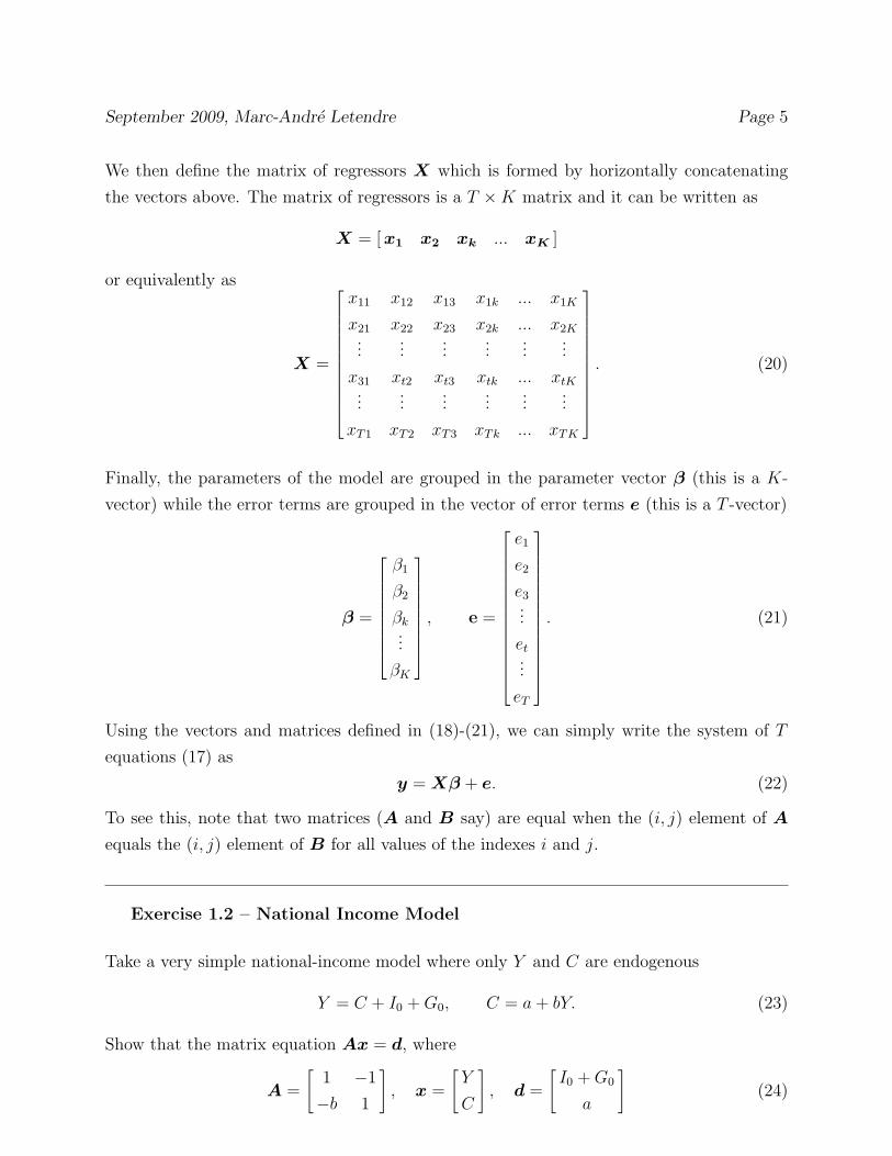
We then define the matrix of regressors X which is formed by horizontally concatenating
the vectors above. The matrix of regressors is a T ×K matrix and it can be written as
X = [ x1 x2 xk ... xK ]
or equivalently as
X =
x11 x12 x13 x1k ... x1K
x21 x22 x23 x2k ... x2K...
......
......
...
x31 xt2 xt3 xtk ... xtK...
......
......
...
xT1 xT2 xT3 xTk ... xTK
. (20)
Finally, the parameters of the model are grouped in the parameter vector β (this is a K-
vector) while the error terms are grouped in the vector of error terms e (this is a T -vector)
β =
β1
β2
βk...
βK
, e =
e1
e2
e3...
et...
eT
. (21)
Using the vectors and matrices defined in (18)-(21), we can simply write the system of T
equations (17) as
y = Xβ + e. (22)
To see this, note that two matrices (A and B say) are equal when the (i, j) element of A
equals the (i, j) element of B for all values of the indexes i and j.
Exercise 1.2 – National Income Model
Take a very simple national-income model where only Y and C are endogenous
Y = C + I0 + G0, C = a + bY. (23)
Show that the matrix equation Ax = d, where
A =
�1 −1
−b 1
�
, x =
�Y
C
�
, d =
�I0 + G0
a
�
(24)

September 2009, Marc-Andre Letendre Page 6
is equivalent to the system of equations (23).
1.4 Special Matrices
A square matrix A is said to be symmetric if its elements are such that aij = aji for all
(i, j) combinations. For a symmetric matrix A, we have A� = A. Here are two symmetric
matrices�
3 7
7 2
�
,
1 2 3
2 5 6
3 6 8
. (25)
A square matrix D is diagonal if its elements are such that dij = 0 for all i �= j. Here
are some diagonal matrices
�1 0
0 3
�
,
2 0 0
0 5 0
0 0 9
,
0 0 0
0 4 0
0 0 11
.
The identity matrix is a special case of a diagonal matrix. The elements on the main
diagonal of the identity matrix are all ones and all the off-diagonal elements are zeroes. The
identity matrix of order n is denoted In. Here are two examples
I2 =
�1 0
0 1
�
, I4 =
1 0 0 0
0 1 0 0
0 0 1 0
0 0 0 1
.
The identity matrix plays a role similar to that of unity in scalar algebra. For example, if
the matrix A is n× n, then InA = A and AIn = A. Also note that the identity matrix is
idempotent (it remains unchanged when it is multiplied by itself any number of times).
Just as the identity matrix plays the role of unity, a null matrix, or zero matrix,
denoted by O plays the role of number zero. Note that contrary to the identity matrix, the
null matrix does not have to be a square matrix. Here are two null matrices�
0 0
0 0
�
,
�0 0 0 0
0 0 0 0
�
. (26)
Triangular matrices have zeros either above the main diagonal (lower-triangular) or
below the main diagonal (upper-triangular).

September 2009, Marc-Andre Letendre Page 7
1.5 Determinants
The determinant of a matrix is particularly useful when we want to determine whether a
matrix is invertible or not. In this subsection we discuss determinants. Matrix inversion is
discussed later in this chapter.
The determinant of a square matrix A, denoted |A| is a uniquely defined scalar asso-
ciated with that matrix. For example, the determinant of a 2× 2 matrix A is calculated as
follows
|A| =
�����a11 a12
a21 a22
����� = a11a22 − a21a12. (27)
Here is a numerical example
A =
�2 3
5 −7
�
, |A| =
�����2 3
5 −7
����� = 2(−7)− 3(5) = −14− 15 = −29. (28)
Whereas calculating second-order determinants as in (28) is easy, the calculation of
higher-order determinants can be a burdensome task. To calculate higher-order determi-
nants, we use a method called Laplace expansion.1 The determinant of a square matrix
A of dimension n is
|A| =n�
j=1
aij |Cij| or |A| =n�
i=1
aij |Cij|. (29)
where |Cij| is the cofactor of element aij.2 To understand what is the cofactor of element
aij, we must first introduce the concept of minor of element aij, denoted |Mij|. |Mij| is a
subdeterminant of |A| obtained by deleting the ith row and the jth column of |A|. A cofactor
is simply a minor with a prescribed algebraic sign attached to it
|Cij| ≡ (−1)i+j|Mij|. (30)
Let’s apply formula (29) to calculate a third-order determinant. We want to find the
determinant of the 3× 3 matrix
A =
5 6 1
2 3 0
7 −3 0
. (31)
1The explanation of the calculation of higher-order determinants is included in these notes for complete-ness and is of secondary importance.
2In equation (29), the formula on the left corresponds to a Laplace expansion by the ith row while theformula on the right corresponds to an expansion by the jth column. Since the determinant of a matrix is aunique number, it does not matter which row or column is used to perform the expansion.

September 2009, Marc-Andre Letendre Page 8
An expansion by the first row yields
|A| = 5(−1)1+1
�����3 0
−3 0
����� + 6(−1)1+2
�����2 0
7 0
����� + 1(−1)1+3
�����2 3
7 −3
����� = −27. (32)
Note that the determinant of a diagonal matrix is simply the product of all the elements
on the main diagonal of the matrix. This implies that (i) the identity matrix always has a
determinant equal to unity and, (ii) any diagonal matrix with a zero on the main diagonal
has a determinant equal to zero. We conclude this subsection by stating six properties of
determinants.
1. The interchange of rows and columns does not affect the value of a determinant. In other
words, |A| = |A�|.
2. The interchange of any two rows (or any two columns) will alter the sign, but not the
numerical value, of the determinant.
3. The multiplication of any one row (or one column) by a scalar k will change the value of
the determinant k-fold.
4. The addition (subtraction) of a multiple of any row to (from) another row will leave the
value of the determinant unaltered. The same holds true if we replace “row” by “column”
in the previous statement.
5. If one row (or column) is a multiple of another row (or column), the value of the deter-
minant will be zero. As a special case of this, when two rows (or columns) are identical, the
determinant will be zero.
6. The expansion of a determinant by alien cofactors (the cofactors of a “wrong” row or
column) always yields a value of zero.
1.6 Rank of a Matrix
The rank of a matrix A indicates the maximum number of linearly independent columns
(or rows) in A. If a matrix A is m × n, then the rank of A can be at most m or n. Put
differently, if we let r(A) denote the rank of matrix A, then
r(A) ≤ min[m,n]. (33)

September 2009, Marc-Andre Letendre Page 9
Note that matrix A is said to be of full rank if r(A) = min[m, n].
For the product of two matrices A and B we have
r(AB) ≤ min [r(A), r(B)] . (34)
As an important practical application, recall the matrix of regressors X that was defined
in the discussion leading to (22). This matrix is T ×K where we restrict T > K. Therefore,
this matrix is full rank when r(X) = K meaning that all regressors (columns) are linearly
independent. Another important property of the rank of a matrix is that r(X �X) = r(X).
Noting that X�X is K ×K, then we have that X
�X is full rank when X is full rank.
To calculate the rank of a matrix we have to find out the number of linearly independent
rows and columns. Consider the following matrix
A =
2 5
3 2
5 7
. (35)
Since it has three rows and two columns, we know that it has rank no greater than 2. By
inspection, we see that the rows of A are not linearly independent (row 3=row 1+row 2)
whereas the two columns of A are. Therefore, r(A) = 2 in this example.
Another example is
B =
2 3
4 6
14 21
. (36)
Again we know that the rank is at most 2. Here we have only one independent row as row
2=2*row 1 and row 3=row 1+3*row 2 and we have only one independent column as column
2=1.5*column 1. So r(B) = 1.
A legitimate question at this point is how do we proceed more generally to calculate the
rank of a matrix? Suppose you are given a matrix A which is m × n where n < m. The
strategy to follow is to find the largest square submatrix of A which has linearly independent
rows and columns.3 If that submatrix is p×p then r(A) = p. For example, if A is 5×4, then
start by looking at 4×4 submatrices of A to see if there is one that has linearly independent
columns and rows. If there is one then r(A) = 4 otherwise look at 3× 3 submatrices of A.
3Submatrices are constructed by omitting some of the rows and columns of the matrix.

September 2009, Marc-Andre Letendre Page 10
If you find a 3×3 submatrix that has linearly independent columns and rows then r(A) = 3
otherwise look at 2× 2 submatrices of A and so on.
If you are used to working with determinants, then you can calculate the rank of a matrix
by using the property that the rank of a matrix A is the dimension of the largest square
submatrix of A whose determinant is not equal to zero.
1.7 Matrix Inversion
The inverse of matrix A, denoted A−1, is defined only if A is a square matrix, in which case
the inverse is the matrix that satisfies the conditions
AA−1 = A
−1A = I. (37)
Not all square matrices are invertible. In the case where A is a square matrix (n × n say),
A is invertible if and only if it has full rank (that is r(A) = n). A square matrix that is not
full rank is said to be singular and hence, is not invertible.4
Here are a few properties of inverses: (A−1)−1 = A; (A�)−1 = (A−1)�; A−1
A = I, where
I is the identity matrix.
The inverse of an invertible matrix A is denoted A−1 and can be calculated as
A−1 =
1
|A| adj(A) (38)
where adj(A) denotes the adjoint of A. Note that the adjoint of A is the transpose of the
matrix of cofactors of A (adj(A)=[cof(A)]�). For the special case where the matrix to invert
is 2× 2, then the previous formula reduces to
�a b
c d
�−1
= (ad− bc)−1
�d −b
−c a
�
. (39)
The inverse of a diagonal matrix is trivial to calculate. We simply have to invert each
of the elements on the main diagonal. For example, for a 3× 3 diagonal matrix D we have
d11 0 0
0 d22 0
0 0 d33
−1
=
1/d11 0 0
0 1/d22 0
0 0 1/d33
. (40)
4In terms of determinants. A matrix with a determinant equal to zero is said to be singular and hence,is not invertible. However, a matrix with a determinant different from zero is nonsingular and is invertible.
September 2009, Marc-Andre Letendre Page 11
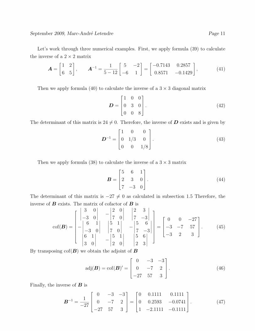
Let’s work through three numerical examples. First, we apply formula (39) to calculate
the inverse of a 2× 2 matrix
A =
�1 2
6 5
�
, A−1 =
1
5− 12
�5 −2
−6 1
�
=
�−0.7143 0.2857
0.8571 −0.1429
�
, (41)
Then we apply formula (40) to calculate the inverse of a 3× 3 diagonal matrix
D =
1 0 0
0 3 0
0 0 8
. (42)
The determinant of this matrix is 24 �= 0. Therefore, the inverse of D exists and is given by
D−1 =
1 0 0
0 1/3 0
0 0 1/8
. (43)
Then we apply formula (38) to calculate the inverse of a 3× 3 matrix
B =
5 6 1
2 3 0
7 −3 0
. (44)
The determinant of this matrix is −27 �= 0 as calculated in subsection 1.5 Therefore, the
inverse of B exists. The matrix of cofactor of B is
cof(B) =
�����3 0
−3 0
����� −�����2 0
7 0
�����
�����2 3
7 −3
�����
−�����
6 1
−3 0
�����
�����5 1
7 0
����� −�����5 6
7 −3
����������6 1
3 0
����� −�����5 1
2 0
�����
�����5 6
2 3
�����
=
0 0 −27
−3 −7 57
−3 2 3
. (45)
By transposing cof(B) we obtain the adjoint of B
adj(B) = cof(B)� =
0 −3 −3
0 −7 2
−27 57 3
. (46)
Finally, the inverse of B is
B−1 =
1
−27
0 −3 −3
0 −7 2
−27 57 3
=
0 0.1111 0.1111
0 0.2593 −0.0741
1 −2.1111 −0.1111
. (47)

September 2009, Marc-Andre Letendre Page 12
1.8 Additional Exercises
Exercise 1.3
Given the matrices and vector below, compute A�, b
�, A−1, AI2, I2A, I2b, Ab, AA, b
�b,
and bb�.
I2 =
�1 0
0 1
�
, A =
�3 1
−2 2
�
, b =
�2
3
�
.
Exercise 1.4
Find the inverse of each of the following matrices:
E =
4 −2 1
7 3 3
2 0 1
, F =
1 −1 2
1 0 3
4 0 2
, G =
1 0 0
0 3 0
0 0 2
Exercise 1.5
For the regression model y = Xβ + e, suppose
X�X =
�50 30
30 84
�
X�y =
�180
60
�
Compute β = (X �X)−1
X�y, the OLS estimates of the parameter vector β.
Exercise 1.6
Consider the constant-returns-to-scale Cobb-Douglas production function Yt = Kat L1−a
t ,
where Y is output and K and L are capital and labour inputs respectively. A popular
econometric model is
ln Yt = β1 + β2 ln Kt + β3 ln Lt + et
where the constant-returns-to-scale assumption is not imposed (i.e. β2 and β3 are not re-
stricted to sum up to unity). The observations on capital and labour inputs (both logged)
are grouped in the matrix of regressors X that also includes a constant regressor. The

September 2009, Marc-Andre Letendre Page 13
observations on output (logged) are grouped in the vector of dependent variables y.
X =
1 2.3 2.5
1 3.3 3.4
1 3.2 3.1
1 3.1 3.1
1 2.7 2.8
1 2.9 3.0
1 2.3 2.4
1 3.2 3.3
1 3.0 3.1
1 3.0 3.1
y =
2.4
3.5
3.1
3.3
2.7
3.0
2.3
3.1
2.9
3.0
• Compute β = (X �X)−1X
�y, the OLS estimates of the parameter vector β.
Exercise 1.7
(a) Find the transpose and the inverse of
A =
�4 2
1 3
�
.
(b) Find the inverse of
B =
3 0 0
0 5 0
0 0 7
.
(c) Find the determinant and the matrix of cofactors of
C =
7 2 −3
5 3 6
0 1 0
.
(d) Calculate the product �4 2
1 3
� �2 −1 −2
5 2 1
�
.
Exercise 1.8
Consider an open economy described by the following equations
Y = C + I + G + X (1)

September 2009, Marc-Andre Letendre Page 14
C = a0 + a1Yd (2)
Y d = (1− τ)Y (3)
X = b0 − b1Y (4)
where Y , I, G, C, X and Y d denote income, investment, government spending, consump-
tion, net exports and disposable income respectively. τ , ai and bi for i = 1, 2 are constant
parameters. Note that we assume I and G are exogenous variables.
(a) Eliminate Y d from the system (1)-(4) and then use matrix notation to write a system of
equations in the remaining endogenous variables Y , C and X. Your system must be of the
form Az = h were z = [ Y C X ]�.
(b) Suppose that a0 = 100, a1 = 0.9, b0 = 100, b1 = 0.12, τ = 0.2, I = 200 and G = 200.
Find the inverse of matrix A and solve for the value of the vector z.
Exercise 1.9
Let X and y be defined as
X =
1 2
1 3
1 4
, y =
4
2
3
1. Calculate X�X.
2. Calculate the rank of X and that of X�X and explain how you get to your answer.
3. Calculate the inverse of X�X.
4. Write down a 3× 4 matrix that is not full rank and explain why it is not full rank.

September 2009, Marc-Andre Letendre Page 15
1.9 Solutions to Exercises
Solution to Exercise 1.3
A� =
�3 −2
1 2
�
, b� = [ 2 3 ] , A
−1 =
�0.25 −0.125
0.25 0.375
�
,
AI2 = A, I2A = A, I2b = b,
Ab =
�9
2
�
, AA =
�7 5
−10 2
�
, b�b = 13, bb
� =
�4 6
6 9
�
Solution to Exercise 1.4
E−1 =
0.375 0.250 −1.125
−0.125 0.250 −0.625
−0.750 −0.500 3.250
, F−1 =
0.0 −0.2 0.3
−1.0 0.6 0.1
0.0 0.4 −0.1
,
G−1 =
1/1 0 0
0 1/3 0
0 0 1/2
Solution to Exercise 1.5
β = [ 4.0364 −0.7273 ]�.
Solution to Exercise 1.6
β = [−0.1077 0.6587 0.3783 ]�.
Solution to Exercise 1.7
(a)
A� =
�4 1
2 3
�
, A−1 =
�0.3 −0.2
−0.1 0.4
�
(b)
B =
1/3 0 0
0 1/5 0
0 0 1/7
.
(c)
|C| = −57, cof(C) =
−6 0 5
−3 0 −7
21 −57 11

September 2009, Marc-Andre Letendre Page 16
(d) �18 0 −6
17 5 1
�
Solution to Exercise 1.8
(a)
1 −1 −1
−a1(1− τ) 1 0
b1 0 1
Y
C
X
=
I + G
a0
b0
(b)
A−1 =
2.5 2.5 2.5
1.8 2.8 1.8
−0.3 −0.3 0.7
, z = A−1
h =
1, 500
1, 180
−80
.
Solution to Exercise 1.9
(a) �3 9
9 29
�
(b) rank(X)≤ (2, 3). Both columns of X are linearly independent. Therefore, rank(X)=2.
rank(X �X)=rank(X)=2.
(c) |X �X| = 6
(X �X)−1 =
1
6
�29 −9
−9 3
�
(d) Let matrix A be
A =
1 3 5 7
1 3 5 7
1 3 5 7
Since all rows of A are identical they are evidently not independent. Therefore the rank of
this matrix is 1. The rank of the matrix would have to be 3 for it to be full rank.
September 2009, Marc-Andre Letendre Page 17
2 Some Probability Concepts
2.1 Random Variables and PDFs
Almost all economic variables are random variables. A random variable is a variable
whose value is unknown until it is observed. The notational convention is to denote random
variables by uppercase letters (e.g. X or Y ) and outcomes of these random variables by
lowercase letters (e.g. x or y).
Random variables are either discrete or continuous. A discrete random variable can
take only a finite number of values (e.g. gender, age, number of years of schooling). A
continuous random variable can take any real value in an interval on the real number
line (e.g. stock returns, GDP growth rates).
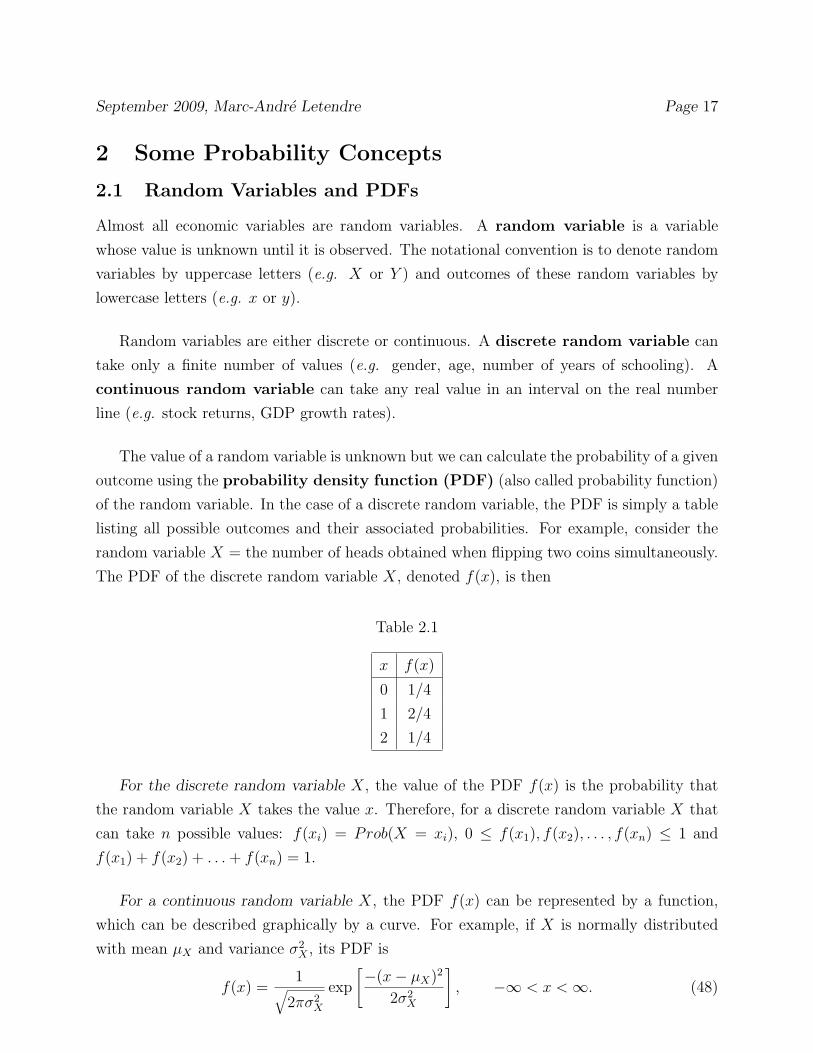
The value of a random variable is unknown but we can calculate the probability of a given
outcome using the probability density function (PDF) (also called probability function)
of the random variable. In the case of a discrete random variable, the PDF is simply a table
listing all possible outcomes and their associated probabilities. For example, consider the
random variable X = the number of heads obtained when flipping two coins simultaneously.
The PDF of the discrete random variable X, denoted f(x), is then
Table 2.1
x f(x)
0 1/4
1 2/4
2 1/4
For the discrete random variable X, the value of the PDF f(x) is the probability that
the random variable X takes the value x. Therefore, for a discrete random variable X that
can take n possible values: f(xi) = Prob(X = xi), 0 ≤ f(x1), f(x2), . . . , f(xn) ≤ 1 and
f(x1) + f(x2) + . . . + f(xn) = 1.
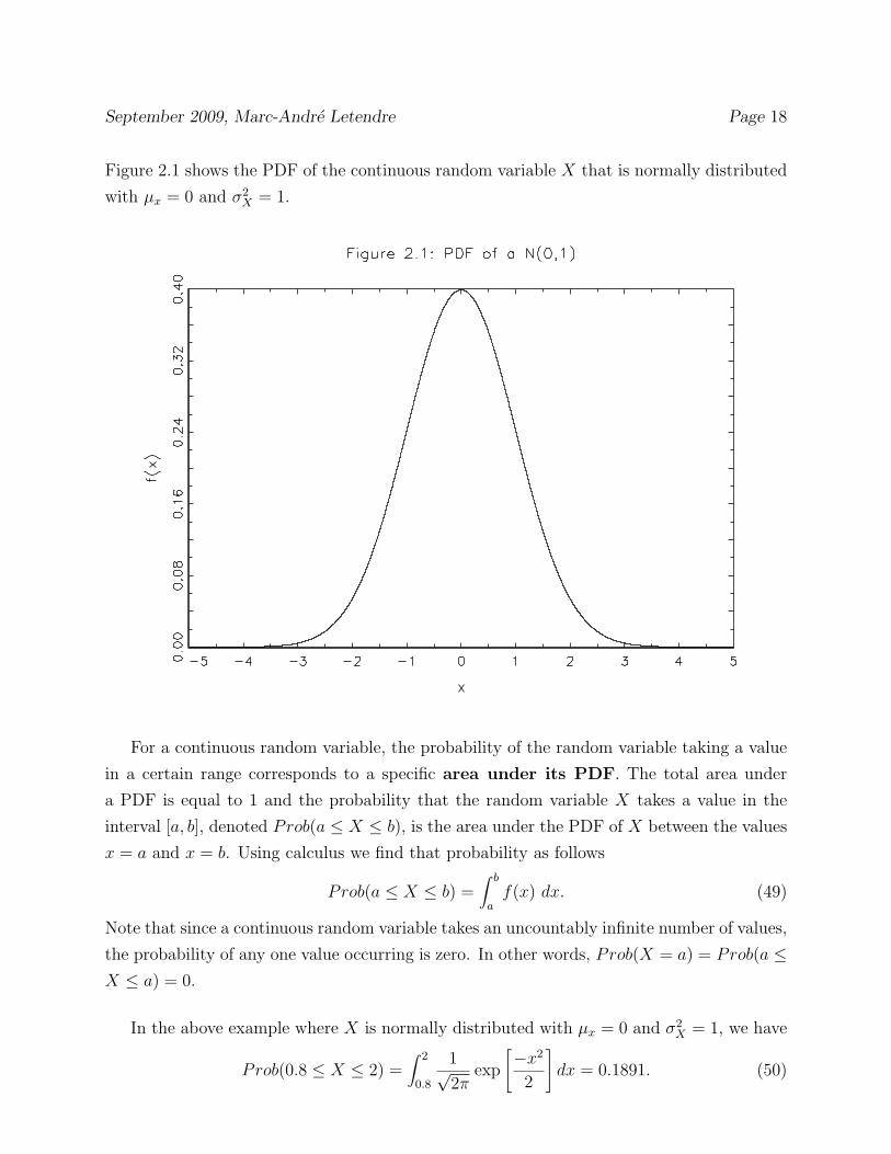
For a continuous random variable X, the PDF f(x) can be represented by a function,
which can be described graphically by a curve. For example, if X is normally distributed
with mean µX and variance σ2X , its PDF is
f(x) =1
�2πσ2
X
exp
�−(x− µX)2
2σ2X
�
, −∞ < x <∞. (48)
September 2009, Marc-Andre Letendre Page 18
Figure 2.1 shows the PDF of the continuous random variable X that is normally distributed
with µx = 0 and σ2X = 1.
For a continuous random variable, the probability of the random variable taking a value
in a certain range corresponds to a specific area under its PDF. The total area under
a PDF is equal to 1 and the probability that the random variable X takes a value in the
interval [a, b], denoted Prob(a ≤ X ≤ b), is the area under the PDF of X between the values
x = a and x = b. Using calculus we find that probability as follows
Prob(a ≤ X ≤ b) =� b
af(x) dx. (49)
Note that since a continuous random variable takes an uncountably infinite number of values,
the probability of any one value occurring is zero. In other words, Prob(X = a) = Prob(a ≤X ≤ a) = 0.
In the above example where X is normally distributed with µx = 0 and σ2X = 1, we have
Prob(0.8 ≤ X ≤ 2) =� 2
0.8
1√2π
exp
�−x2
2
�
dx = 0.1891. (50)

September 2009, Marc-Andre Letendre Page 19
2.2 Moments of Random Variables2.2.1 Rules of Summation
The formulae calculating the moments of random variables are more conveniently written
using summation notation. Therefore we first review the rules of summation. In equations
(51)-(58) below, X and Y are random variables and a and b are constants. X can take n
possible values and Y can take m possible values where m ≥ n.
1.
x1 + x2 + . . . + xn =n�
i=1
xi. (51)
2.n�
i=1
a = n a. (52)
3.n�
i=1
axi = an�
i=1
xi. (53)
4.n�
i=1
(xi + yi) =n�
i=1
xi +n�
i=1
yi. (54)
5.n�
i=1
(a + bxi) = n a + bn�
i=1
xi. (55)
6.n�
i=1
(axi + byi) = an�
i=1
xi + bn�
i=1
yi. (56)
7. The arithmetic mean (average) of T realizations of the random variable X is
x =x1 + x2 + . . . + xT
T=
1
T
T�
i=1
xi. (57)
8. The order of summation does not matter
n�
i=1
m�
j=1
f(xi, yi) =m�
j=1
n�
i=1
f(xi, yi). (58)
We sometimes use abbreviated forms of the summation operator. For example suppose that
X can take n possible values. Instead of�n
i=1 f(xi) we could write�
i f(xi) which reads

September 2009, Marc-Andre Letendre Page 20
“sum over all values of the index i”. Or alternatively,�
x f(x) which reads “sum over all
possible values of X.”
Exercise 2.1 – Summation Operator
Express each of the following sums using the summation operator
(a) y1 + y2 + y3 + y4 + y5 + y6
(b) ax1 + bx2 + cx3 + dx4
(c) ax1 + ax2 + ax3 + ax4
(d) y1 + x1 + y2 + x2 + y3 + x3 + x4 + y4
Exercise 2.2 – Summation Operator
Using the sample of data
t 1 2 3 4 5
xt 2 3 7 0 9
yt 4 10 1 5 6Calculate the following
(a)�5
t=1 yt
(b)�4
t=2 xt
(c)�5
t=1 xtyt
(d)�5
t=1 xt�5
t=1 yt
(e)�5
t=1 x2t
(f) (�5
t=1 xt)2
2.2.2 Expectation, Variance and the Expectation Operator
The first moment of a random variable is its mean or expectation. The expectation of
a random variable X is the average value of the random variable in an infinite number of
repetitions of the experiment (or in repeated samples). We denote the expectation of X by
E[X].
If X is a discrete random variable with associated PDF f(x), then the expectation of X
is
E[X] =�
x
x f(x). (59)
September 2009, Marc-Andre Letendre Page 21
For example, using the PDF in Table 2.1 we have
E[X] =�
x
x f(x) = 0× 1/4 + 1× 1/2 + 2× 1/4 = 1. (60)
It is important to distinguish an expectation from a sample average. To illustrate the
difference, consider our example where X = the number of heads obtained when flipping
two coins simultaneously. The expectation of X is equal to 1 as shown in equation (60).
Suppose that we repeat the experiment three times and get the outcomes: Head-Tail, Tail-
Head and Head-Head. Therefore the three realizations of X in our sample are 1, 1 and 2.
The sample average is x = (1 + 1 + 2)/3 = 4/3. In general, the sample average will differ
from the expectation, as it is the case in this example. However, if we repeat the experiment
an infinite number of times, then the sample average will be equal to the expectation in
accordance with the definition of an expectation given at the beginning of this subsection.5
In the case of a continuous random variable, the expectation is calculated as
E[X] =�
x f(x) dx. (61)
To calculate the expectation of a function g(X) of random variable X, we apply
the formula
E[g(X)] =�
x
g(x)f(x) (62)
when X is a discrete random variable and
E[g(X)] =�
g(x) f(x) dx (63)
when X is a continuous variable.
Note that in general E[g(X)] �= g(E[X]]). We will come back to this below.
To illustrate how to apply formula (62), let us use the PDF of the discrete random
variable X displayed in Table 2.1 to calculate E[3X2].
E[3X2] = (3× 02)1
4+ (3× 12)
1
2+ (3× 22)
1
4= 4.5. (64)
5To convince yourself, repeat the experiment a large number of times. After each repetition, recalculatethe sample mean. You will see that as the number of repetitions gets large, the sample mean converges tothe expectation.

September 2009, Marc-Andre Letendre Page 22
Here are some properties of the expectation operator. They are all relatively easy
to show.6 Let a and c denote constants and X denote a random variable:
1. The expectation of a constant
E[c] = c. (65)
2. Multiplying a random variable by a constant
E[cX] = cE[X]. (66)
3. Expectation of a sum. Let g1(X) and g2(X) be functions of the random variable X,
then
E[g1(X) + g2(X)] = E[g1(X)] + E[g2(X)]. (67)
4. Combining the previous properties
E[a + cX] = a + cE[X]. (68)
Often times, economic models imply taking the expectation of non-linear functions. For
example, in ECON 723 we often deal with Euler equations. These equations involve taking
the expectation of a marginal utility function which is usually non-linear. It turns out that
if g() is a concave function we have E[g(X)] ≤ g(E[X]) whereas we have E[g(X)] ≥ g(E[X])
if g() is a convex function. This is Jensen’s inequality. Let’s prove Jensen’s inequality for
the case where g() is convex and differentiable. We first use the convexity of g(X) to write
g(x) ≥ g(µX) + g�(µX)(x− µX), ∀x (69)
where µX = E[X] and g�(x) = ∂g(x)/∂x. Combining equations (62) and (69) we have
E[g(X)] =�
x
g(x)f(x) ≥�
x
[g(µX) + g�(µX)(x− µX)]f(x). (70)
It is straightforward to show that the term to the right of the inequality sign is equal to
g(µX) = g(E[X])
�
x
[g(µX) + g�(µX)(x− µX)]f(x) =�
x
g(µX)f(x) +�
x
g�(µX)(x− µX)f(x) (71)
= g(µX) + g�(µX)�
x
xf(x)− g�(µX)µX = g(µX) + g�(µX)µX − g�(µX)µX = g(µX)
6Doing so is an excellent exercise.

September 2009, Marc-Andre Letendre Page 23
Combining (70) and (71) completes the proof that E[g(X)] ≥ g(E[X]).
Exercise 2.3 – Jensen’s Inequality
Suppose that a representative agent has utility function u(Y ) = ln(Y ) where Y denotes
consumption. Suppose that consumption has the following PDF
Table 2.2
y f(y)
2 0.35
3 0.25
4 0.40
The expected marginal utility of consumption is E[1/Y ]. Show that E[1/Y ] �= 1/E[Y ] in
this numerical example.
We complete this section by discussing the second moment of a random variable, its
variance. The variance of a random variable X is defined as
var(X) = E(X − E[X])2. (72)
Note that the symbol σ2 is often used to denote the variance (and the symbol σ to denote
the standard deviation) of a random variable.
The variance of a function g(X) of random variable X is calculated as
var(g(X)) = E(g(X)− E[g(X)])2. (73)
While the expectation provides information about the center of the distribution of a
random variable, the variance provides information about the spread of the distribution.
Figure 2.2 compares the PDFs of two random variables: X is normally distributed with
expectation 0 and variance 1, and Y is normally distributed with expectation 0 and variance
5. We see that both PDFs are centered around zero but that the PDF of Y (dotted line) is
“flatter”.

September 2009, Marc-Andre Letendre Page 24
We can use equation (62) to re-write the variance formula
var(X) = E(X − E[X])2 =�
x
f(x)(x− E[X])2 (74)
where f(x) is the PDF of the discrete random variable X.
Exercise 2.4 – Variance of Consumption and Marginal Utility
Using the PDF in Table 2.2, calculate the variance of consumption (Y ) and marginal utility
(1/Y ).
Just like the expectation operator, the variance operator has many properties. The ones
listed below are all relatively easy to show.7 Let a and c denote constants and X denote a
random variable:7Doing so is an excellent exercise.

September 2009, Marc-Andre Letendre Page 25
1. The variance of a constant is zero
var(a) = 0. (75)
2. Multiplying a r.v. by a constant multiplies its variance by the square of the constant
var(cX) = c2var(X). (76)
3. Combining properties 1 and 2
var(a + cX) = c2var(X). (77)
2.3 Several Random Variables2.3.1 Joint, Marginal and Conditional PDFs
To make probability statements about more than one random variable we must know their
joint probability density function (or joint PDF). The joint PDF of two continuous
random variables must be represented on a three-dimensional graph. The volume under the
surface of the joint PDF is equal to 1.
The joint PDF of two discrete random variables, Y1 and Y2 say, is a table reporting
possible outcomes of the two variables with their joint probabilities. For example, consider a
two-period economy where consumption in period 1 (Y1) and consumption in period 2 (Y2)
are random variables with joint PDF
Table 2.3: f(y1, y2) — Joint PDF of Y1 and Y2
y1\y2 2 3 4
2 0.20 0.15 0.05
4 0.05 0.15 0.40
The joint PDF above indicates that the probability that the agent consumes 2 units in
period 1 and 3 units in period 2 is f(2, 3) = 0.15. The probability that the agent consumes
4 units in period 1 and 4 units in period 2 is f(4, 4) = 0.40. The concept of joint PDF is not
limited to the binary case. For example, if Y1, Y2, . . . , Ym are random variables, then their
joint PDF is denoted f(y1, y2, . . . , ym).

September 2009, Marc-Andre Letendre Page 26
We calculate the expectation of a function of several random variables using a
formula similar to that displayed in equation (62). Again, let Y1 and Y2 denote two discrete
random variables with joint PDF f(y1, y2) and let g(Y1, Y2) denote a function of Y1 and Y2.
Then we have
E[g(Y1, Y2)] =�
y1
�
y2
g(y1, y2)f(y1, y2). (78)
If Y1 and Y2 are continuous random variables, then
E[g(Y1, Y2)] =�
y1
�
y2
g(y1, y2)f(y1, y2) dy1 dy2. (79)
Exercise 2.5 – Expected Consumption Growth
Using the joint PDF in Table 2.3, calculate expected gross consumption growth between
periods 1 and 2.
Given a joint PDF, we can calculate marginal PDFs and conditional PDFs. A marginal
PDF indicates the probability of an individual random variable.8 Let Y1 and Y2 be two
discrete random variables. To calculate the marginal PDF of Y1 (denoted f(y1)) using the
joint PDF f(y1, y2) we “sum out” the other variable (Y2)
f(y1) =�
y2
f(y1, y2). (80)
And similarly
f(y2) =�
y1
f(y1, y2). (81)
If Y1 and Y2 are continuous random variables we have
f(y1) =�
f(y1, y2) dy2, f(y2) =�
f(y1, y2) dy1. (82)
Coming back to the two-period consumption example. The marginal PDFs of Y1 and Y2 are
8So in a sense, the PDF displayed in Table 2.1 is a marginal PDF. The notation reflects this fact.
September 2009, Marc-Andre Letendre Page 27
Table 2.4 Marginal PDF of Y1 (period 1 consumption)
y1 f(y1)
2 0.40
4 0.60
Table 2.5 Marginal PDF of Y2 (period 2 consumption)
y2 f(y2)
2 0.25
3 0.30
4 0.45
Table 2.4 indicates that the consumer will consume 2 units in period 1 with a probability
of 0.40. Table 2.5 indicates that the consumer will consume 3 units in period 2 with a
probability of 0.30.
A conditional probability is the probability of an event conditional on the realization
of another event. Consider the case of two discrete random variables, Y1 and Y2. Condi-
tional probabilities are calculated from the joint PDF f(y1, y2) and the marginal PDF of
the conditioning random variable. Prob[Y2 = y2|Y1 = y1] denotes the probability that the
random variable Y2 takes the value y2 given that the random variable Y1 takes the value y1.
We denote the conditional PDF by f(y2|y1) and calculate it as follows
f(y2|y1) = Prob[Y2 = y2|Y1 = y1] =f(y1, y2)
f(y1)(83)
In the two-period consumption example, suppose we want to know the probability that the
agent consumes 3 units in period 2 given that he consumes 2 units in period 1. We calculate
the probability as
Prob(Y2 = 3|Y1 = 2) =Prob(Y1 = 2, Y2 = 3)
Prob(Y1 = 2)=
0.15
0.40= 0.375. (84)
Note that we could also calculate Prob(Y1 = y1|Y2 = y2) if we wanted to.
In the two-period consumption example, the PDF of the random variable Y2 conditional
on Y1 = 4 is

September 2009, Marc-Andre Letendre Page 28
Table 2.6 PDF of Y2 conditional on Y1 = 4
y2 f(y2|4)
2 0.05/0.60=0.0833
3 0.15/0.60=0.2500
4 0.40/0.60=0.6667
2.3.2 Statistical Independence
We say that two random variables are statistically independent, or independently
distributed, if knowing the value that one takes does not reveal anything about what value
the other may take.
When the random variables Y1 and Y2 are statistically independent, their joint PDF is
the product of their marginal PDFs, that is
f(y1, y2) = f(y1)f(y2). (85)
Similarly, if the random variables Y1, Y2, . . . , Yn are statistically independent their joint PDF
is
f(y1, y2, . . . , yn) = f(y1)f(y2) · · · f(yn) (86)
Combining (83) and (85) we find that if Y1 and Y2 are statistically independent random
variables then the conditional PDFs reduce to marginal PDFs
f(y2|y1) =f(y1, y2)
f(y1)=
f(y1)f(y2)
f(y1)= f(y2), f(y1|y2) =
f(y1, y2)
f(y2)=
f(y1)f(y2)
f(y2)= f(y1).
(87)
In the two-period consumption example, the random variable Y1 and Y2 are not statistically
independent. Notice how marginal and conditional PDFs differ by comparing tables 2.5 and
2.6.
2.3.3 Conditional Expectation and Variance
With the conditional PDF of a random variable on hand, we can calculate conditional
moments (e.g. conditional expectation and conditional variance). For example, using the

September 2009, Marc-Andre Letendre Page 29
conditional PDF in Table 2.6 we can calculate the expectation and variance of the random
variable Y2 conditional on Y1 = 4
E[Y2|Y1 = 4] = 2×Prob(Y2 = 2|Y1 = 4)+3×Prob(Y2 = 3|Y1 = 4)+4×Prob(Y2 = 4|Y1 = 4)
(88)
= 2× 0.0833 + 3× 0.25 + 4× 0.6667 = 3.5833,
var(Y2|Y1 = 4) = E[Y2 − E(Y2|Y1 = 4)]2 = (2− 3.5833)2 × Prob(Y2 = 2|Y1 = 4) (89)
+(3− 3.5833)2 × Prob(Y2 = 3|Y1 = 4)
+(4− 3.5833)2 × Prob(Y2 = 4|Y1 = 4) = 0.4097.
Exercise 2.6 – Bond Returns
Suppose that in the two-period economy example the gross return on a one-period real bond,
denoted RY1=y1 , is related to consumption as follows
1
RY1=y1
= 0.95 E
�Y1
Y2
�����Y1 = y1
�
(90)
where the subscript on R reminds us that the return is conditional on the value of consump-
tion in period 1.
Using the PDF in Table 2.3, calculate the two possible values for the conditional return R
and then calculate the unconditional expected bond return Re
2.3.4 Covariance and Correlation
To measure how closely two variables move together, we calculate their covariance defined
as
cov(Y1, Y2) = E[(Y1 − E[Y1])(Y2 − E[Y2])]. (91)
The expression in square brackets in equation (91) is an example of a function of Y1 and Y2.
Therefore, we can combine equations (78) and (91) to write
cov(Y1, Y2) = E[(Y1 − E[Y1])(Y2 − E[Y2])] =�
y1
�
y2
(y1 − E[Y1])(y2 − E[Y2]) f(y1, y2) (92)
September 2009, Marc-Andre Letendre Page 30
when Y1 and Y2 are discrete random variables and equations (79) and (91) to write
cov(Y1, Y2) = E[(Y1 − E[Y1])(Y2 − E[Y2])] =�
y1
�
y2
(y1 − E[Y1])(y2 − E[Y2]) f(y1, y2) dy1 dy2
(93)
when Y1 and Y2 are continuous random variables.
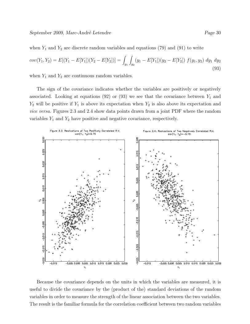
The sign of the covariance indicates whether the variables are positively or negatively
associated. Looking at equations (92) or (93) we see that the covariance between Y1 and
Y2 will be positive if Y1 is above its expectation when Y2 is also above its expectation and
vice versa. Figures 2.3 and 2.4 show data points drawn from a joint PDF where the random
variables Y1 and Y2 have positive and negative covariance, respectively.
Because the covariance depends on the units in which the variables are measured, it is
useful to divide the covariance by the (product of the) standard deviations of the random
variables in order to measure the strength of the linear association between the two variables.
The result is the familiar formula for the correlation coefficient between two random variables
September 2009, Marc-Andre Letendre Page 31
Y1 and Y2
cor(Y1, Y2) =cov(Y1, Y2)�
var(Y1) var(Y2). (94)
The correlation coefficient lies in the interval [−1, 1]. When cor(Y1, Y2) equals 1 (−1), we
say that the variables Y1 and Y2 are perfectly positively (negatively) correlated.
Note that if the random variables Y1 and Y2 are statistically independent, then their
covariance and correlation are zero. However, the converse is not true.
Exercise 2.7 – Covariance and Correlation
Use the joint PDF in Table 2.3 to calculate the covariance and correlation of the random
variables Y1 and Y2.
2.3.5 Expectation and Variance of a Sum of Random Variables
This short subsection lists a few important rules regarding expectations and variances of a
sum of random variables. They can all be derived from equation (78).9 Let Y1 and Y2 be
random variables and a and b be constants. The rules are
1. Expectation of a weighted sum of random variables
E[aY1 + bY2] = aE[Y1] + bE[Y2]. (95)
2. Variance of a weighted sum of random variables
var(aY1 + bY2) = a2var(Y1) + b2var(Y2) + 2ab cov(Y1, Y2). (96)
3. Expectation of a product of random variables
E[aY1 bY2] = ab E[Y1] E[Y2] + ab cov(Y1, Y2). (97)
In the special case where Y1 and Y2 are independent or uncorrelated we have
var(aY1 + bY2) = a2var(Y1) + b2var(Y2), E[aY1 bY2] = ab E[Y1] E[Y2]. (98)
9Doing so is an excellent exercise.

September 2009, Marc-Andre Letendre Page 32
These rules generalized to the case where there is more than two random variables. For
example, let c denote a constant and Y3 a random variable. Then we have
E[aY1 + bY2 + cY3] = aE[Y1] + bE[Y2] + cE[Y3] (99)
and
var(aY1 + bY2 + cY3) = a2var(Y1) + b2var(Y2) + c2var(Y3) + 2ab cov(Y1, Y2) (100)
+2ac cov(Y1, Y3) + 2bc cov(Y2, Y3).
2.3.6 Random Vectors and Matrices
Closely related to the concepts of expectation, variance and covariance of scalar random vari-
ables is that of the expectation of a random vector or matrix and the variance-covariance
matrix of a vector of random variables.
Recall the vector of error terms in (21). Denote the expectation of element ei as E[ei] = µi
and let µ = [ µ1 µ2 . . . µT ]�. The expectation of a vector (or matrix) is calculated by
taking the expectation of each element inside the vector (or matrix). Therefore we have
E[e] =
E[e1]
E[e2]
E[e3]...
E[eT ]
=
µ1
µ2
µ3...
µT
= µ (101)
By definition, the variance-covariance matrix of e is
Var(e) = E [(e− E[e])(e− E[e])�] . (102)
The variance-covariance matrix has variances of the random variables on the main diagonal
and covariance terms on the off diagonal. To see this work out Var(e) when e is a column-
vector with two elements.10
In the context of the linear regression model where we assume E[e] = 0 formula (102)
simplifies to Var(e) = E [ee�].
10Start by working out the product (e − E[e])(e − E[e])� then calculate the expectation of each elementof the resulting matrix.

September 2009, Marc-Andre Letendre Page 33
Let A be a matrix containing deterministic elements. Suppose that the number of
columns of A matches the number of rows of e. Then the variance-covariance matrix of
the product Ae is
Var(Ae) = E[(Ae− E(Ae))(Ae− E(Ae))�] = E[A(e− E(e))(e− E(e))�A�] (103)
= AE[(e− E(e))(e− E(e))�]A� = AVar(e)A�
where we make use of the property E[Ae] = AE[e] which can easily be derived from (66).
Make sure you understand all steps of the derivation in (103). Notice how the variance-
covariance formula in (103) differs from that of the scalar case shown in (76).
2.4 Markov Chains
Acknowledgement: this section draws heavily from Ljungqvist and Sargent (2004) chapter 2.
2.4.1 A Few Definitions
A stochastic process is a sequence of random variables. We denote a sequence of random
variables by {Xt} where X denotes a random variable and t denotes a time index (when
time is discrete t is an integer). When relevant, the exact starting and ending values of the
time index are specified. For example, if the context is such that the time index can only
take integer values from 1 and 50 then we write {Xt}50t=1.
A Markov chain is a stochastic process that satisfies the Markov property. Ljungqvist
and Sargent (2004) provide the following definition: A stochastic process {Xt} is aid to have
the Markov property if for all k ≥ 1 and all t,
Prob(xt+1|xt, xt−1, xt−2, . . . , xt−k) = Prob(xt+1|xt). (104)
Interpreting X as a state variable11, then the Markov property means that given the current
state (xt), the realization of the next period state (xt+1) is uncorrelated with past realizations
(xt−1, xt−2 and so forth). When the order of the Markov chain is not specified, it is to be
11A classical example given to illustrate the concept of state of the world is the weather: in period t iteither rains or shine (two possible states of the world).

September 2009, Marc-Andre Letendre Page 34
understood that the chain is of the first-order (as defined above). In the case of a second-order
Markov chain (104) must be replaced by
Prob(xt+1|xt, xt−1, xt−2, . . . , xt−k) = Prob(xt+1|xt, xt−1). (105)
A Markov chain is said to be time-invariant (or time-homogenous) if
Prob(xt+h+1|xt+h) = Prob(xt+1|xt), ∀h > 0. (106)
From now on, we work with first-order time-invariant Markov chains. Such a chain is defined
by a triplet of objects.
(i) An n-dimensional state space consisting of vectors ei for i = 1, . . . , n where ei is a
unit vector where the ith element is equal to unity and all other elements equal zero.
For example, if there are three possible states of the world then n = 3 (e.g. the GDP
growth rate is zero, positive or negative) and the state space is defined by
e1 =
1
0
0
, e2 =
0
1
0
, e3 =
0
0
1
. (107)
(ii) An n × n transition matrix P containing the transition probabilities, that is, the
probabilities of moving from one value of the state space to another in one period. The
ijth element of P is Pij = Prob(Xt+1 = ej|Xt = ei). Note that P does not have any
kind of time dependency here because we focus on time-invariant Markov chains.
Continuing with our n = 3 example we have
P =
P11 P12 P13
P21 P22 P23
P31 P32 P33
=
Prob(Xt+1 = e1|Xt = e1) Prob(Xt+1 = e2|Xt = e1) Prob(Xt+1 = e3|Xt = e1)
Prob(Xt+1 = e1|Xt = e2) Prob(Xt+1 = e2|Xt = e2) Prob(Xt+1 = e3|Xt = e2)
Prob(Xt+1 = e1|Xt = e3) Prob(Xt+1 = e2|Xt = e3) Prob(Xt+1 = e3|Xt = e3)
(108)
Matrix P satisfies condition�n
j=i Pij = 1 which makes it a stochastic matrix, that
is, a matrix that defines the probabilities of moving from each value of the state space
to any other in one period.
(iii) A vector of marginal probabilities in period 0 (the initial period) for the n elements of
the state space. Let π0 denote this column vector. Its ith element is π0i = Prob(X0 =
ei). The vector π0 satisfies�n
i=1 = π0i = 1

September 2009, Marc-Andre Letendre Page 35
2.4.2 Stationarity
Once the Markov chain is defined, the transition matrix containing the probabilities of
moving from each value of the state space to any other in k periods is given by Pk (to
illustrate this work out exercise 2.16) and the vector of unconditional probabilities in any
period are calculated as
(t = 1) π�1 = Prob(X1) = π
�0P (109)
(t = 2) π�2 = Prob(X2) = π
�0P
2
...
(t = k) π�k = Prob(Xk) = π
�0P
k
where π�t = Prob(Xt) is 1 × n and has ith element πti = Prob(Xt = ei). Generalizing the
equation for t = 1 above we see that unconditional probability distributions evolve according
to
π�t+1 = π
�tP . (110)
For example, when n = and t = 1 the above equation becomes
[ π21 π22 ] = [ π11 π12 ]
�P11 P12
P21 P22
�
= [ π11P11 + π12P21 π11P12 + π12P22 ] (111)
The unconditional distribution is said to be stationary or invariant if it satisfies πt+1 =
πt = π. From equation (110) a stationary distribution must satisfy
π� = π
�P ⇒ π
�(I − P ) = 0 (112)
Let’s denote the probability distribution the Markov chain will converge to in the infinite
future by π∞ = limt→∞ πt. Then we have a definition and a theorem regarding asymptotic
stationarity in section 2.2.2 of Ljungqvist and Sargent.
Definition: Let π∞ be a unique vector that satisfies π�(I − P ) = 0 [i.e π∞ is a stationary
distribution]. If for all distributions π0 it is true that limt→∞Pt�π0 converges to the same
π∞, we say that the Markov chain is asymptotically stationary with a unique invariant
distribution. Then, we call π∞ a stationary distribution of P .
Theorem: Let P be a stochastic matrix with Pij > 0 ∀(i, j). Then P has a unique stationary
distribution, and the process is asymptotically stationary.
The theorem states that as long as the transition probabilities are positive, then Pt�π0 will
eventually converge to a unique π.

September 2009, Marc-Andre Letendre Page 36
2.4.3 Expectations
We terminate our introduction to Markov chains by revisiting the concept of expectations.
Let’s first think about E[Xt] =�n
i=1 xiπti. Given the way the x�is are defined we obviously
get E[Xt] = πt = Pt�π0. Therefore, when the Markov chain is stationary then so is E[Xt].
Suppose we are interested in a variable Y which is related to the state X as follows:
Yt = X �ty where y is an n × 1 vector of real numbers. Given the way we defined the state
space for X, we know that Yt = yi when Xt = ei. The unconditional expectation of Yt is
then E[Yt] = π�ty = π
�0P
ty (make sure you can derive this).
Finally, the conditional expectation of Yt+1 given that the state in period t is xt = ei
is simply the ith row of matrix P y. That is, E[Yt+1|Xt = ei] = (P y)i. For a two-step-
ahead forecast we have E[Yt+2|Xt = ei] = (P 2y)i and for a k-step-ahead forecast we have
E[Yt+k|Xt = ei] = (P ky)i.
Therefore, once the transition matrix P and initial distribution π0 are known it is trivial to
calculate the conditional and unconditional probability of Yt+k, k > 0
E[Yt+k] = π�0P
t+ky and E[Yt+k|Xt] = P
ky (113)
where the last expression comes from “stacking” the expectations E[Yt+k|Xt = ei] = (P ky)i
for i = 1, . . . , n.

September 2009, Marc-Andre Letendre Page 37
2.5 Additional Exercises
Exercise 2.8
Consider a two-period economy where consumption in period t is given by Yt where t = 1, 2.
Consumption in both periods is random and its joint PDF is
y1\y2 2 3 4
2 0.20 0.08 0.04
3 0.08 0.20 0.08
4 0.04 0.08 0.20
(a) Calculate the expectation and the variance of Y1.
(b) Let lifetime utlity be U = ln(Y1)+0.9 ln(Y2). Calculate the expectation and the variance
of U .
(c) Given that Y1 = 3, calculate E[U |Y1 = 3].
(d) Calculate cov(Y1, Y2) and cor(Y1, Y2).
(e) Are the random variable Y1 and Y2 statistically independent in this example?
Exercise 2.9
Let Y1 and Y2 be two discrete random variales. Use Jensen’s inequality to find whether
E�Y1
Y2|Y1 = y1
�× E
�Y2
Y1|Y1 = y1
�
is less, greater or equal to 1.
Exercise 2.10
Let Y1 and Y2 be two discrete random variales. Prove that
var(Y1 + Y2) = var(Y1) + var(Y2) + 2 cov(Y1, Y2).
Exercise 2.11
Consider a two-period economy where consumption in period i is given by Yi where i = 1, 2.
Consumption in both periods is random and its PDF is

September 2009, Marc-Andre Letendre Page 38
y1\y2 2 3 4
1 0.10 0.08 0.02
3 0.50 0.10 0.20
(a) Calculate the expectation and the variance of Y1.
(b) Verify whether the marginal PDF of Y2 is equal to the PDF of Y2 conditional on Y1 = 3.
(c) Let lifetime utlity be U = Y1Y2. Calculate the expectations E[U ] and E[U |Y1 = 3].
Exercise 2.12
Let Y1 and Y2 be two discrete random variables and let a and b be two constants. The
marginal PDF of Yi is denoted f(yi) and the PDF of Y2 conditional on Y1 = y1 is denoted
f(y2|y1).
(a) Show that E[aY1 + bY2] = aE[Y1] + bE[Y2].
(b) Show that var(aY2) = a2var(Y2).
(c) Show that f(y2|y1) = f(y2) if Y1 and Y2 are statistically independent.
(difficult) Show that E{E[Y2|Y1 = y1]} = E[Y2].
Exercise 2.13
Let a = 2, b = 3 and c = 4. The following table lists the joint probabilities for the values of
two random variables, X and Y .
Y = 1 Y = 2 Y = 3
X = 1 0.15 0.05 0.20
X = 2 0.10 0.40 0.10
Calculate the following probabilities:
(a) Pr(Y = 1)
(b) Pr(X = 2)
(c) Pr(X = 2|Y = 1)
(d) Pr(Y = 1|X = 1)
Calculate the following expectations:

September 2009, Marc-Andre Letendre Page 39
(e) E[X]
(f) E[Y ]
(g) E[XY ]
(h) E[X|Y = 1]
(i) E[a + bX]
Calculate the following variances and covariances:
(j) V ar[X]
(k) V ar[aX + bY ]
(l) Cov[X,Y ]
(m) Cov[a + bX, cY ]
Exercise 2.14
Let X1 and X2 be two discrete random variables and let a and b be two constants. The joint
probability density function (PDF) of X1 and X2 is denoted f(X1, X2).
(a) Prove that
var(aX1 + bX2) = a2var(X1) + b2var(X2) + 2ab cov(X1, X2).
(b) Prove that cov(X1, X2) = 0 if X1 and X2 are statistically independent.
Exercise 2.15
Consider a two-period economy where consumption in period i is given by Yi where i = 1, 2.
Consumption in both periods is random and its PDF is
y1\y2 3 4 5
2 0.35 0.15 0.10
4 0.10 0.05 0.25
(a) Calculate the variance of Y2 conditional on Y1 = 4.
(b) Verify whether the random variables Y1 and Y2 are statistically independent.
Exercise 2.16 – Calculating a transition matrix
Suppose there are two states of the world. Write down matrix P for the case n = 2 and
then calculate P 2. Using a probability tree, verify that the elements of your matrix P 2 are
correct.
September 2009, Marc-Andre Letendre Page 40
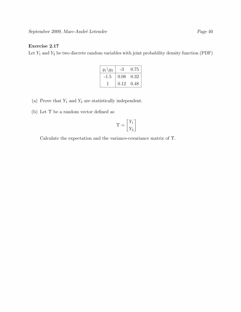
Exercise 2.17
Let Y1 and Y2 be two discrete random variables with joint probability density function (PDF)
y1\y2 -3 0.75
-1.5 0.08 0.32
1 0.12 0.48
(a) Prove that Y1 and Y2 are statistically independent.
(b) Let Υ be a random vector defined as
Υ =
�Y1
Y2
�
Calculate the expectation and the variance-covariance matrix of Υ.
September 2009, Marc-Andre Letendre Page 41
2.6 Solutions to Exercises
Solution to Exercise 2.1
(a) y1 + y2 + y3 + y4 + y5 + y6 =�6
t=1 yt
(b) x1y2 + x2y3 + x3y4 + x4y5 + x5y6 =�5
t=1 xtyt+1 or�6
t=2 xt−1yt
(c) ax1 + ax2 + ax3 + ax4 =�4
t=1 axt or a�4
t=1 xt
(d) y1 + x1 + y2 + x2 + y3 + x3 + x4 + y4 =�4
t=1 xt +�4
t=1 yt
(e) x21 + x2
2 + x23 + x2
4 + (y1 + y2 + y3)2 =�4
t=1 x2t + (
�3t=1 yt)2
Solution to Exercise 2.2
(a)�5
t=1 yt = 26
(b)�4
t=2 xt = 10
(c)�5
t=1 xtyt = 99
(d)�5
t=1 xt�5
t=1 yt = 546
(e)�3
t=1 x2t = 62
(f) (�3
t=1 xt)2 = 144
(g)�4
t=1(xt/yt) = 7.8
(h) (�4
t=2 xt)/(�5
t=1 yt) = 0.3846
Solution to Exercise 2.3
In this question, we have E[Y ] = 3.05 and therefore 1/E[Y ] = 0.3279. However, applying
formula (62) we find
E[1/Y ] = (1/2)× 0.35 + (1/3)× 0.25 + (1/4)× 0.40 = 0.3583 > 1/E[Y ].
Solution to Exercise 2.4
Before calculating the variances, we need the expectations. From Exercise 2.3 we have
E[Y ] = 3.05 and E[1/Y ] = 0.3583. The variance of consumption is
var(Y ) = (2− 3.05)2 × 0.35 + (3− 3.05)2 × 0.25 + (4− 3.05)2 × 0.40 = 0.7475
and the variance of marginal utility is
var(1/Y ) = (1/2−0.3583)2×0.35+(1/3−0.3583)2×0.25+(1/4−0.3583)2×0.40 = 0.0119.
Solution to Exercise 2.5
Let the function g(Y1, Y2) denote the consumption (gross) growth rate. That is, g(Y1, Y2) =
Y2/Y1. Applying formula (78) we find
E[g(Y1, Y2)] =2
2× 0.20 +
3
2× 0.15 +
4
2× 0.05 +
2
4× 0.05 +
3
4× 0.15 +
4
4× 0.40 = 1.0625.

September 2009, Marc-Andre Letendre Page 42
Solution to Exercise 2.6
If Y1 = 2 then,
1
RY1=2= 0.95 E
�Y1
Y2
�����Y1 = 2
�
= 0.95�2
2× 0.5 +
2
3× 0.375 +
2
4× 0.125
�= 0.8125
and therefore RY1=2 = 1.2308.
If Y1 = 4 then,
1
RY1=4= 0.95 E
�Y1
Y2
�����Y1 = 4
�
= 0.95�4
2× 0.0833 +
4
3× 0.25 +
4
4× 0.6667
�= 1.1083
and therefore RY1=4 = 0.9023.
The marginal PDF of Y1 tells us that there is a 40 percent probability that the conditional
return takes a value 1.2308 and a 60 percent chance that its takes a value 0.9023. Accordingly,
the unconditional expectation of the conditional return is
Re ≡ E[RY1=y1 ] = 0.40× 1.2308 + 0.60× 0.9023 = 1.0337.
Note that you can also get to the answer
Re = 1.0337
by using the property E[E(X2|X1 = x1)] = E(X2) for any two random variables X1 and X2.
Solution to Exercise 2.7
cov[Y1, Y2] = 0.46 and cor[Y1, Y2] = 0.5779.
Solution to Exercise 2.8
(a) E[Y1] = 3, var[Y1] = 0.64.
(b) The distribution of the random variable U is

September 2009, Marc-Andre Letendre Page 43
u f(u)
1.316980 0.20
1.681898 0.08
1.722445 0.08
1.940812 0.04
2.010127 0.04
2.087363 0.20
2.346277 0.08
2.375045 0.08
2.633959 0.20
E[U ] = 2.015751, var[U ] = 0.210210.
(c) E[U |Y1 = 3] = 2.0638.
(d) cov[Y1, Y2] = 0.32 and cor[Y1, Y2] = 0.5.
(e) No. Two random variables that are statistically independent are always uncorrelated.
Solution to Exercise 2.9
E�Y1
Y2|Y1 = y1
�× E
�Y2
Y1|Y1 = y1
�
= E�
1
Y2|Y1 = y1
�× E [Y2|Y1 = y1]
defining g(x) = 1/x we can write
=E[g(Y2)|Y1 = y1]
g(E[Y2|Y1 = y1])≥ 1
since g(x) = 1/x is a convex function.
Solution – Exercise 2.10
Let µ1 ≡ E[Yi] for i = 1, 2.
var(Y1 + Y2) =�
y1
�
y2
[y1 + y2 − µ1 − µ2]2f(y1, y2)
=�
y1
�
y2
[(y1 − µ1) + (y2 − µ2)]2f(y1, y2)
=�
y1
�
y2
[(y1 − µ1)2 + 2(y1 − µ1)(y2 − µ2) + (y2 − µ2)
2]f(y1, y2)

September 2009, Marc-Andre Letendre Page 44
=�
y1
(y1 − µ1)2f(y1) + 2cov(Y1, Y2) +
�
y2
(y2 − µ2)2f(y2)
= var[Y1] + 2cov(Y1, Y2) + var[Y2].
Solution – Exercise 2.11
(a) E[Y1] = 2.6; var[Y1] = 0.64.
(b) Marginal PDF of Y2
y2 f(y2)
2 0.60
3 0.18
4 0.22
Marginal PDF of Y2 conditional on Y1 = 3
y2 f(y2)
2 0.625
3 0.115
4 0.25
Marginal PDF of Y2 is not equal to the conditional PDF of Y2 conditional on Y1 = 3.
(c) E[U ] = 6.82; E[U |Y1 = 3] = 7.875.
Solution – Exercise 2.13
(a) Pr(Y = 1) = 0.25
(b) Pr(X = 2) = 0.6
(c) Pr(X = 2|Y = 1) = 0.4
(d) Pr(Y = 1|X = 1) = 0.375
(e) E[X] = 1.6
(f) E[Y ] = 2.05
(g) E[XY ] = 3.25
(h) E[X|Y = 1] = 1.4
(i) E[a + bX] = 6.8
(j) V ar[X] = 0.24
(k) V ar[Y ] = 0.5475
(l) Cov[X,Y ] = −0.03
(m) V ar[aX + bY ] = 5.5275
(n) Cov[a + bX, cY ] = −0.36
September 2009, Marc-Andre Letendre Page 45
Solution – Exercise 2.15
(a) E[Y2|Y1 = 4] = 4.375 and var(Y2|Y1 = 4) = 0.734375.
(b) Statistical independence implies that marginal and conditional PDFs are identical.
Showing that f(Y2) �= f(Y2|Y1 = 4) is sufficient to conclude that Y1 and Y2 are not in-
dependent.
Solution – Exercise 2.16
P 2 =
�p2
11 + p12p21 p11p12 + p12p22
p21p11 + p22p21 p21p12 + p222
�
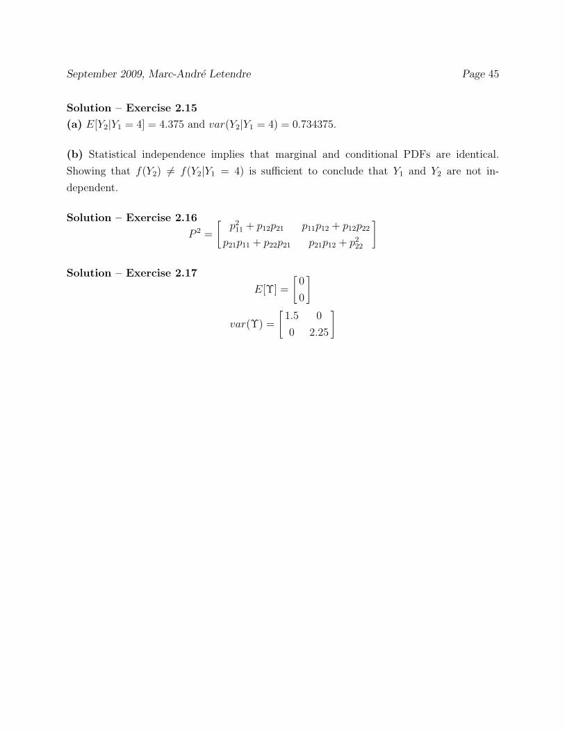
Solution – Exercise 2.17
E[Υ] =
�0
0
�
var(Υ) =
�1.5 0
0 2.25
�

September 2009, Marc-Andre Letendre Page 46
3 Difference Equations
Many economic models give rise to difference equations. It is therefore important to know
some of the techniques available to solve them. We restrict our attention to first-order and
second-order difference equations. This choice is not as restrictive as it may seem given that
a very large number of models generate first or second-order difference equations.
When dealing with difference equations it is implicitly assumed that time is discrete.12
That is, the “time variable” t takes values like . . . ,−3,−2,−1, 0, 1, 2, 3, . . .. In general, t can
run from −∞ to +∞. You can think of t as indexing months or quarters. For example,
t = 0 could represent the first quarter of 1947, t = 1 the second quarter of 1947 and so on.
The general form of an nth-order linear difference equation in the variable y is
yt = a0 +n�
i=1
aiyt−i + xt (114)
where a0, . . . , an are constant coefficients and xt is called a forcing process and can be any
function of time, current and lagged values of other variables, and/or stochastic disturbances.
In solving a difference equation, the objective is to find a time path for the variable y.
This time path is represented by the sequence {yt}∞t=0 (often simply denoted {yt}). The time
path we are looking for should be a function of t (i.e. a formula defining the values of y in
every time period) which is consistent with the given difference equation as well as with its
initial conditions. Also, the time path must not contain any difference expression such as
∆yt. Note that I denote first differences as ∆yt ≡ yt − yt−1. You should be careful about
the ∆ notation since some authors prefer defining first differences as ∆yt ≡ yt+1 − yt.
Most of this chapter discusses linear difference equations. In a linear difference equation,
no y term (of any period) is raised to a power different from unity or is multiplied by a y
term of another period.
3.1 First-Order Difference Equations3.1.1 Solution by Iteration
If we are provided with a first-order difference equation and an initial condition (i.e. a
known value for y0), then we can simply iterate forward from that initial period to calculate
12When time is continuous, we use the expression differential equation.
September 2009, Marc-Andre Letendre Page 47
the entire time path for y. Consider the linear first-order stochastic difference equation
yt = a0 + a1yt−1 + �t (115)
where �t is a random variable. Given an initial condition y0 and a realization for �1, we can
calculate y1 by setting t = 1 in (115)
y1 = a0 + a1y0 + �1. (116)
Similarly, setting t = 2 in (115) and using (116) we have
y2 = a0 + a1y1 + �2 = a0 + a1[a0 + a1y0 + �1] + �2 = a0(1 + a1) + a21y0 + a1�1 + �2. (117)
One more iteration yields
y3 = a0 + a1
�a0(1 + a1) + a2
1y0 + a1�1 + �2
�+ �3 (118)
= a0(1 + a1 + a21) + a3
1y0 + a21�1 + a1�2 + �3.
The solutions for y1, y2 and y3 above make clear that further iterations will yield
yt = a0
t−1�
i=0
ai1 + at
1y0 +t−1�
i=0
ai1�t−i (119)
Consider a first numerical example where an initial condition y0 is given, the parameters
are a0 = 0 and a1 = 0.95 and finally xt = 0 for all t. The equation to use to calculate the
time path for y is then
yt = 0.95yt−1. (120)
Again, let’s iterate on (120) three times to identify a pattern we can generalize. A first
iteration yields y1 = 0.95y0. A second iteration yields y2 = 0.95y1 = 0.952y0 and a third
iteration yields y3 = 0.95y2 = 0.953y0. Clearly, the solution to the deterministic homogeneous
linear first-order difference equation (120) is yt = 0.95ty0.
As a second example, consider the (non-homogeneous) difference equation
yt = 1 + 0.95yt−1. (121)
where an initial condition y0 is provided. A first iteration yields y1 = 1 + 0.95y0. A second
iteration yields
y2 = 1 + 0.95y1 = 1 + 0.95[1 + 0.95y0] = 1 + 0.95 + 0.952y0.
September 2009, Marc-Andre Letendre Page 48
A third iteration yields
y3 = 1 + 0.95y2 = 1 + 0.95[1 + 0.95 + 0.952y0] = 1 + 0.95 + 0.952 + 0.953y0.
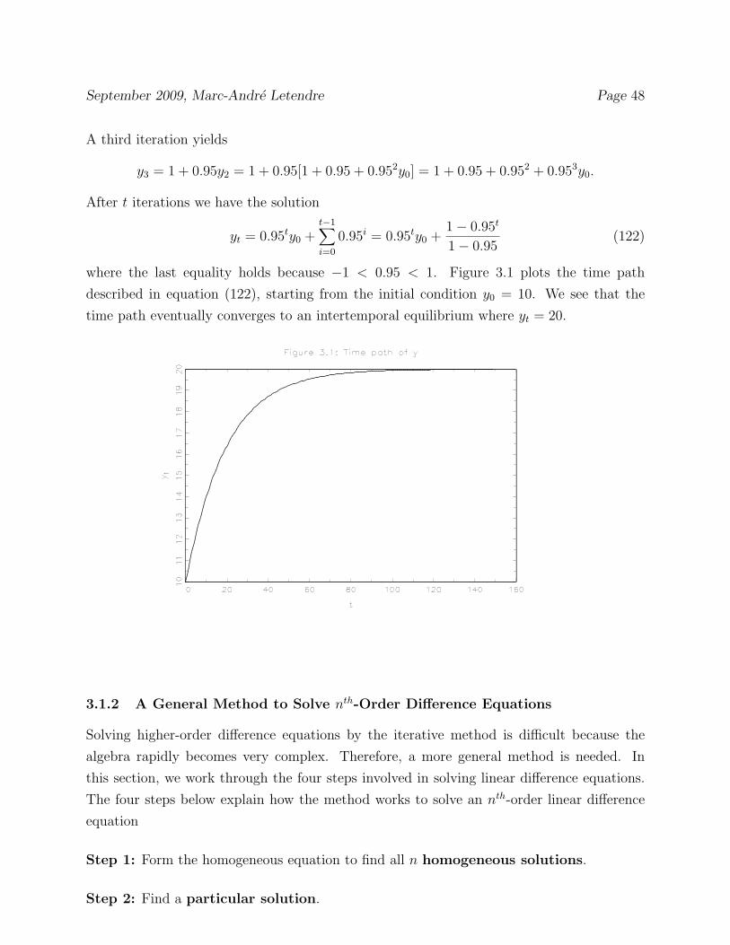
After t iterations we have the solution
yt = 0.95ty0 +t−1�
i=0
0.95i = 0.95ty0 +1− 0.95t
1− 0.95(122)
where the last equality holds because −1 < 0.95 < 1. Figure 3.1 plots the time path
described in equation (122), starting from the initial condition y0 = 10. We see that the
time path eventually converges to an intertemporal equilibrium where yt = 20.
3.1.2 A General Method to Solve nth-Order Difference Equations
Solving higher-order difference equations by the iterative method is difficult because the
algebra rapidly becomes very complex. Therefore, a more general method is needed. In
this section, we work through the four steps involved in solving linear difference equations.
The four steps below explain how the method works to solve an nth-order linear difference
equation
Step 1: Form the homogeneous equation to find all n homogeneous solutions.
Step 2: Find a particular solution.
September 2009, Marc-Andre Letendre Page 49
Step 3: Obtain the general solution as the sum of the particular solution and a linear
combination of all homogeneous solutions.
Step 4: Eliminate the arbitrary constant(s) by imposing the initial condition(s) on the
general solution to get the definite solution.13
The particular solution is any solution of the complete nonhomogeneous equation (114).
The homogeneous solution, denoted yh, is the general solution of the homogeneous version
of (114) given by
yt =n�
i=i
aiyt−i. (123)
The particular solution represents the intertemporal equilibrium level of y while the
combination of homogeneous solutions represents the deviations of the time path from that
equilibrium.
To see how the method works we apply it to solve the first-order linear difference equation
(FOLDE)
yt+1 = a0 + a1yt. (124)
In step 1, we find the solution to the homogeneous equation
yt+1 = a1yt. (125)
We guess that the solution to (125) is of the form
yt = Aαt (126)
where A and α are unknown coefficients. If our guess is correct it must also be the case that
yt+1 = Aαt+1. We find the value of α by substituting the guess on both sides of (125) to get
Aαt+1 = a1Aαt. (127)
Dividing through by Aαt yields α = a1. Using this result in our guess (126) implies that the
homogeneous solution should be written as
yht = Aat
1. (128)
13Note that some authors refer to the “homogeneous solutions” as the “complementary function”, to the“particular solution” as the “particular integral” and to the “general solution” as the “arbitrary solution.”

September 2009, Marc-Andre Letendre Page 50
In step 2, we have to find a particular solution to equation (124). Remember that the
particular solution is any solution to the complete nonhomogeneous equation. Therefore, let
us use a simple trial solution where y is constant over time. That is yt = c for all t. Using
this trial solution in (124) we can solve for c
c = a0 + a1c ⇒ c =a0
1− a1(129)
when a1 �= 1. Therefore, the particular solution can be written as
yp =a0
1− a1, (a1 �= 1). (130)
Obviously if a1 = 1, then a0/(1− a1) is not defined and some other particular solution must
be found. When a1 = 1, we use the trial solution yt = ct. Substituting this trial solution on
both sides of (124) we can solve for c
c(t + 1) = a0 + a1ct, ⇒ c =a0
1 + t− a1t. (131)
Given that a1 = 1 we find c = a0 and therefore, the particular solution is
ypt =
�a0/(1− a1), if a1 �= 1
a0t, if a1 = 1. (132)
In step 3 we combine homogeneous and particular solutions to obtain the general solution.
In the present case the general solution is written as
yt =
�Aat
1 + a01−a1
, if a1 �= 1
A + a0t, if a1 = 1(133)
In step 4 we find the value of the unknown coefficient A using the general solution and the
initial condition y0. Setting t = 0 in the general solution (133) yields
y0 = A +a0
1− a1⇒ A = y0 −
a0
1− a1, a1 �= 1 (134)
y0 = A ⇒ A = y0, a1 = 1. (135)
Using these results in the general solution (133) yields the definite solution
yt =
� �y0 − a0
1−a1
�at
1 + a01−a1
, if a1 �= 1
y0 + a0t, if a1 = 1(136)
Let us apply the four-step general method to a numerical example. Suppose that the
first-order difference equation we want to solve and the initial condition on y are
yt+1 = 1 + 0.5yt, y0 = 4. (137)

September 2009, Marc-Andre Letendre Page 51
We first proceed to solve the homogeneous version of (137) which is
yt+1 = 0.5yt. (138)
We guess that a solution to (138) is yt = Aαt. Substituting the guess in (138) yields
Aαt+1 = 0.5Aαt ⇒ α = 0.5 ⇒ yht = A0.5t. (139)
Second, we find a particular solution to (137). Since a1 �= 1 in this example, we guess that
y is constant over time, yt = c. Substituting this guess in (137) yields
c = 1 + 0.5c ⇒ c = 2 ⇒ yp = 2. (140)
Third, we combine the homogeneous and particular solution to get the general solution
yt = A0.5t + 2. (141)
Fourth, we use the initial condition y0 = 4 to identify A. Setting t = 0 in the general solution
(141) yields
4 = y0 = A + 2 ⇒ A = 2. (142)
Therefore, the solution to (137) is
yt = 2× 0.5t + 2. (143)
3.1.3 Dynamic Stability of a FOLDE
Recall that the particular solution to a difference equation represents the intertemporal
equilibrium level of y while the homogeneous solution represents the deviations of the time
path from that equilibrium. Therefore, it is not surprising that the dynamic stability of the
equilibrium depends on whether or not the homogeneous solution tends to zero as t → ∞.
The value of α in the homogeneous solution Aαt governs the time path of Aαt as t→∞.
We consider three cases. First, if |α| < 1 then the expression αt converges to zero as
t → ∞. In the case where −1 < α < 0, the term αt change signs every period. In such a
case, we say that the homogeneous solution displays oscillations.
Second, if |α| > 1 then the expression αt increases with t and the homogeneous solution is
explosive. In the special case where α < −1, the homogeneous solution oscillates explosively.
September 2009, Marc-Andre Letendre Page 52
Third, we have the case where |α| = 1. When α = 1 the homogeneous solution is always
equal to A. This may lead one to conclude that the time path of y will converge since the
homogeneous solutions does not explode. It is not the case however. Note that the time
path of y will converge to A + yp and not to its long run equilibrium level yp (unless A = 0).
Therefore, if we want the time path of y to converge to the equilibrium yp, we have to rule
out the case α = 1. Similarly, the case α = −1 must also be ruled out.
In summary, the solution yt = Aαt + yp is a convergent path if and only if
|α| < 1.
Exercise 3.1 – A Dynamically Stable Case
Apply the four-step method to solve the following difference equation
yt+1 = 1 + 0.95yt, y0 = 25.
Exercise 3.2 – Unit Root
Apply the four-step method to solve the following difference equation
yt+1 = 2 + yt, y0 = 5.
3.1.4 Linearizing Nonlinear Difference Equations
Not all economic models lead to linear difference equations. There are a couple of ways
to deal with nonlinear difference equations. Sometimes a simple operation transforms a
nonlinear difference equation in a linear one. For example, suppose the time path of GDP
(denoted by y) is described by
yt+1 = b0ya1t . (144)
If we are willing to study the dynamic properties of the logarithm of GDP instead of GDP,
then we can take logs on both sides of (144) to get
ln(yt+1) = ln(b0) + a1 ln(yt) (145)

September 2009, Marc-Andre Letendre Page 53
Defining gt = ln(yt), a0 = ln(b0) we end up with a linear difference equation in g
gt+1 = a0 + a1gt. (146)
Obviously, not all nonlinear difference equations have the log-linear form of (144). For
example, if we add a constant term so that yt+1 = b0ya1t + b1, then we cannot take logs to
“linearize” this nonlinear difference equation.
A strategy used regularly in macroeconomics is to approximate nonlinear equations by linear
ones before solving them. Taking a linear approximation yields a linear difference equation
that can be solved and studied in the way presented in the previous sections. To present the
basic idea we focus here on a first-order approximation.
According to Taylor’s Theorem, given an arbitrary function f(y), if we know the value of
the function at y = y and the value of its derivatives at y then
f(y) =
�f(y)
0!+
f �(y)
1!(y − y) +
f ��(y)
2!(y − y)2 + . . . +
f (n)(y)
n!(y − y)n
�
+ Rn (147)
where n denotes the order of the approximation, f (n) denotes the nth derivative of f(−) and
Rn is the remainder term (you can think of it as an approximation error).
When we use a first-order (hence linear) approximation we set n = 1 and drop the remainder
term to write
f(y) ≈ f(y) + f �(y)(y − y). (148)
where we used the fact that 0! = 1 and 1! = 1.
Evidently, when we solve difference equations we have at least two variables (taking time into
account) appearing in the function to approximate (e.g. yt and yt+1) so we have to adapt
the linear approximation to this scenario. Suppose that function f(−) actually depends on
yt and yt+1 as it would in the example
yt+1 = b1yt + b2yb3t . (149)
Then the first-order approximation formula becomes
f(yt, yt+1) ≈ f(y, y) + f1(y, y)(yt − y) + f2(y, y)(yt+1 − y) (150)
where the approximation point is (yt, yt+1) = (y, y) and fi(−) denotes the partial derivative
of f(−) with respect to its ith argument. The natural approximation point is the long run

September 2009, Marc-Andre Letendre Page 54
equilibrium value of y which is usually not that hard to find as long as the difference equation
we are solving is stationary. When it is not, then some intermediate steps must be taken to
arrive at a stationary nonlinear difference equation. Here we sidestep this issue by assuming
that the the equation we want to study (e.g. (149)) is stationary.
To see how the first-order linear approximation method works we approximate (149)). First,
we define the f(−) function which can be written
f(yt, yt+1) ≡ b1yt + b2yb3t − yt+1. (151)
With this definition, equation (149) is written f(yt, yt+1) = 0.
Second, we take the partial derivatives
f1(yt, yt+1) = b1 + b2b3yb3−1t , f2(yt, yt+1) = −1. (152)
Third, we apply formula (150)
f(yt, yt+1) ≈ [(b1 − 1)y + b2yb3 ]
� �� �f(y,y)
+ [b1 + b2b3yb3−1]
� �� �f1(y,y)
(yt − y) + [−1]� �� �f2(y,y)
(yt+1 − y) (153)
Therefore, our approximation of f(yt, yt+1) = 0 is
[(b1 − 1)y + b2yb3 ] + [b1 + b2b3y
b3−1](yt − y) + [−1](yt+1 − y) = 0. (154)
Actually, given that f(−) is defined in such a way that the nonlinear equation being approx-
imated is written f(yt, yt+1) = 0, it is always the case that f(y, y) = 0 which implies that the
first term in the equation above is exactly zero since it is exactly equal to f(y, y) as pointed
out in (153). Taking this into account our approximation of f(yt, yt+1) = 0 is
[b1 + b2b3yb3−1](yt − y) + [−1](yt+1 − y) = 0. (155)
Define a1 ≡ b1 + b2b3yb3−1 and the variables in deviations from their long-run equilibrium
level as gt ≡ yt − y (and gt+1 ≡ yt+1 − y). Then our linearized difference equation is written
gt+1 = a1gt (156)
which has a familiar form.
It is natural to wonder how we actually get the value y we are using in the approximation.
Remember that we are assuming a stationary nonlinear difference equation. Therefore we

September 2009, Marc-Andre Letendre Page 55
know that in the long-run yt = yt+1. We then solve for y by using yt = yt+1 = y in (149)
which yields
y =
�1− b1
b2
� 1b3−1
(157)
As an exercise, approximate the nonlinear difference equation
yt+1 = 0.9yt + y0.5t (158)
to find the equivalent of (156) and then solve.
3.1.5 Nonlinear Difference Equations: a Graphical Approach
When we want to study a nonlinear difference equation without approximating it we can
simply calculate the time path of y by iterating forward on the nonlinear difference equation
starting from an initial condition y0. However, when we do that we may not be able to
figure out the convergence properties of the time path (convergent, divergent, oscillatory).
To figure them out, we make use of a graphical tool: the phase diagram.
To explain what a phase diagram is, let us denote the nonlinear relationship between yt+1
and yt as yt+1 = f(yt). For example in equation (144), f(yt) = b0ya1t . A phase diagram
plots a phase line corresponding to f() together with a 45o line in the (yt+1, yt)-plan. Figure
3.2 plots four phase diagrams. In panels (a) and (b), the phase lines have positive slopes
(everywhere) while they have negative slopes (everywhere) in the other two panels. Starting
from an initial condition y0 on the yt-axis, we use the phase line to find y1, y2 and so on.
This is equivalent to iterating forward on the nonlinear difference equation starting from y0.
In Figure 3.2a, we see that the time path of y will converge to y where y represents the
intertemporal equilibrium level of y and is found at the intersection of the phase line and
the 45o line.14 Note that the time path of y converges to y whether y0 < y or y0 > y.
In Figure 3.2b, we see that the time path of y diverges from its equilibrium level y.15 For
example, if y0 > y then we have y0 < y1 < y2 < y3 < y4 < . . . and the time path will tend
to infinity (divergent path) as t→∞. If y0 < y, then the time path is also divergent but in
the other direction.14Recall that, by definition, yt+1 = yt along the 45o line.15Unless the initial condition turns out to be exactly y0 = y.

September 2009, Marc-Andre Letendre Page 56
In Figure 3.2c, the time path converges to y but is oscillatory. The figure illustrates the
phenomenon of overshooting. That is, if we start with y0 < y, the time path for y will
overshoot its equilibrium level as it converges to it. This is seen in the case illustrated in
Figure 3.2c since starting from y0 < y implies y1 > y.
Finally, Figure 3.2d displays an example of an oscillatory and divergent time path.
As you have most likely realized by now, the convergence properties of the time path
described by a nonlinear difference equation depend on the absolute value of the slope of
f() while the algebraic sign of the slope determines whether there will be oscillations or not.
When the absolute value of the slope is less than unity (as in Figures 3.2a and 3.2c) then
the time path is convergent. When the slope is negative, then the time path is oscillatory.
In general, the phase line may have positively or negatively sloped segments. It may also
have segments where the absolute value of its slope is less than unity and others where it is
greater than unity. In these cases, the time path will be more complicated but it can still
be analyzed using a phase diagram. In these cases, different starting values may imply time

September 2009, Marc-Andre Letendre Page 57
paths that are widely different.
3.1.6 Stochastic Difference Equations and the Method of Undetermined Coef-
ficients
The discussion in subsection 3.1.2 was restricted to deterministic linear difference equa-
tions. This section outlines the method of undetermined coefficients which is useful to find
particular solutions when difference equations include stochastic components. To keep the
exposition relatively clear, we will restrict our attention to solving the first-order stochastic
difference equation
yt+1 = a0 + a1yt + �t+1 (115�)
using an initial condition y0 and where |a1| < 1.
To solve equation (115’) we follow the four steps presented in subsection 3.1.2. The first
step is to find the homogeneous solution by solving
yt+1 = a1yt. (159)
As usual we guess that the homogeneous solution has the form yt = Aαt. Substituting the
guess in the equation above yields α = a1. Therefore the homogeneous solution is Aat1 where
the constant A will be determined in step 4.
In step 2 we have to find a particular solution to equation (115’). This is where the
method of undetermined coefficients comes in. Contrary to the deterministic case, it does
not make sense to choose yt = c (y constant over time) as a trial solution since y depends
on a random variable (�) which is not constant over time. Instead we use the trial solution
yt = c +∞�
i=0
βi�t−i (160)
where c and β0, β1, . . . are undetermined coefficients. If the trial solution is correct, then it
must be the case that
yt+1 = c +∞�
i=0
βi�t+1−i. (161)
Substituting the trial solution (160)-(161) into (115’) yields
c + β0�t+1 + β1�t + β2�t−1 + β3�t−2 + . . . (162)
= a0 + a1 [c + β0�t + β1�t−1 + β2�t−2 + . . .] + �t+1

September 2009, Marc-Andre Letendre Page 58
Re-arranging (162) to collect like terms, we obtain
(c− a0 − c a1) + (β0 − 1)�t+1 + (β1 − a1β0)�t + (β2 − a1β1)�t−1 + . . . = 0 (163)
Since equation (163) must hold for all possible values of the {�t} sequence, each of the
following conditions must hold
β0 − 1 = 0, β1 − a1β0 = 0, β2 − a1β1 = 0, . . . (164)
c− a0 − c a1 = 0 (164a).
We can easily solve for the βi’s recursively from (164): β0 = 1, β1 = a1, β2 = a21, . . ., βi = ai
1.
Then from (164a) we get c = a0/(1 − a1) (recall that we assumed |a1| < 1). Using these
results in the trial solution (160) yields the particular solution
ypt =
a0
1− a1+
∞�
i=0
ai1�t−i. (165)
In step 3 we simply combine the homogeneous and particular solutions (yt = yh + yp)
yt = Aat1 +
a0
1− a1+
∞�
i=0
ai1�t−i. (166)
In the last step, we use the initial condition y0 to identify A. Setting t = 0 in the general
solution (166) yields
y0 = A +a0
1− a1+
∞�
i=0
ai1�−i (167)
which implies that
A = y0 −a0
1− a1−
∞�
i=0
ai1�−i. (168)
Therefore the definite solution to equation (115) is
yt =
�
y0 −a0
1− a1−
∞�
i=0
ai1�−i
�
at1 +
a0
1− a1+
∞�
i=0
ai1�t−i (169)
which after some algebra can be written as
yt =�y0 −
a0
1− a1
�at
1 +a0
1− a1+
t−1�
i=0
ai1�t−i (170)
As you can see, the approach followed to solve a stochastic difference equation resem-
bles that used to solve a deterministic difference equation. The main difference lies in the
identification of the particular solution (step 2).

September 2009, Marc-Andre Letendre Page 59
3.1.7 Forward and Backward-Looking Solutions
The solution (170) to the stochastic difference equation (115’) is what we call a backward-
looking solution since it involves past values of the random variables. Notice that the solution
(119) to (115) obtained by backward repeated substitution is also a backward-looking solu-
tion. Recall that the backward repeated substitution method works as follows: start with
equation (115), then substitute out yt−1 (which introduces a term in yt−2), then substitute
out yt−2 (which introduces a term in yt−3), and so on.
We can also use a forward repeated substitution method which yields a forward-looking
solution. Instead of substituting out lags of yt, we substitute out leads of yt. For example,
we can rewrite equation (115) as
yt−1 = −a0
a1− �t
a1+
yt
a1. (171)
Updating by one period to get yt on the left-hand side yields
yt = −a0
a1− �t+1
a1+
yt+1
a1. (172)
To iterate forward on equation (172) we use the fact that yt+1 = (yt+2 − a0 − �t+2)/a1 to
substitute out yt+1 and get
yt = −a0
a1− �t+1
a1+
1
a1
�yt+2
a1− a0 + �t+2
a1
�. (173)
Re-arranging we have
yt = −a0
a1− a0
a12− �t+1
a1− �t+2
a21
+yt+2
a21
. (174)
Continuing this iterative process yields
yt = −a0
n�
i=1
a−i1 −
n�
i=1
a−i1 �t+i +
yt+n
an1
. (175)
Clearly, if |a1| > 1, the first term in (175) converges to a0/(1 − a1) while the last term
converges to zero as n tends to infinity. Therefore, a particular solution is
yt =a0
1− a1−
∞�
i=1
a−i1 �t+i. (176)
As explained in the discussion around equation (159) the homogeneous solution is yt = Aat1
where A is an unknown constant to be identified in step (4) using the initial condition y0.
It is worth taking some time to discuss some properties the forward-looking particular
solution (176) and of the backward-looking particular solution
yt =a0
1− a1+
∞�
i=0
ai1�t−i. (177)

September 2009, Marc-Andre Letendre Page 60
First, the backward-looking solution depends on past realizations of the random variables
while the forward-looking solution depends on future realizations of the random variables.
Since these future realizations are not observed, it may seem that the forward-looking solu-
tion is of limited interest. As you will see, forward-looking solutions are encountered when
solving rational expectations models. In such models, current behaviour of an economic
agent depends on its expectation of future events. For example, a consumer’s decision re-
garding consumption/savings in period t most likely depends on its expectations of future
income. In such a case, the random variables �t+1, �t+2, . . . appearing in the forward-looking
particular solution (176) would be replaced by their expectations/forecasts conditional on
the information known in period t denoted Et�t+1, Et�t+2, . . ..
Second, let us see how the two solutions depend on a1. Consider the backward-looking
solution first. If |a1| < 1, the expression ai1 converges toward zero as i → ∞ which implies
that the effects of past random variables diminishes over time when |a1| < 1. This can be
interpreted two ways: (1) the effect of �t−2 on yt is smaller than the effect of �t−1 on yt;
(2) the effect of �t−1 on yt is larger than its effect on yt+1. However, if |a1| > 1 then the
backward-looking solution explodes since the expression ai1 converges to infinity as i → ∞
(see the discussion in subsection 3.1.3).
The image is reversed when dealing with the forward-looking solution. If |a1| < 1, then
the expression a−i1 tends to infinity as i →∞ and the forward-looking solution explodes. If
|a1| > 1, then the expression a−i1 tends to zero as i → ∞ and the forward-looking solution
yields a finite sequence {yt}. When |a1| > 1, the effects of future random variables diminishes
over time. This can be interpreted two ways: (1) the effect of �t+2 on yt is smaller than the
effect of �t+1 on yt; (2) the effect of �t+2 on yt+1 is larger than its effect on yt.
From a purely mathematical point of view, we cannot say whether the forward-looking
or backward-looking solution is most appropriate. However economic theory often suggests
that a sequence be bounded (i.e. the elements of the sequence cannot tend to infinity).16
In such a case, we use the forward-looking solution when |a1| > 1 and the backward-looking
solution when |a1| < 1. In higher order difference equations where we may have stable
(inside the unit circle) and unstable roots (outside the unit circle) we often solve stable roots
backwards and unstable roots forwards.16For example, we do not expect real returns on assets, real GDP per capita and several other economic
variables to tend to (plus or minus) infinity.
September 2009, Marc-Andre Letendre Page 61
3.2 Vector First-Order Difference Equations
A vector difference equation differs from the difference equations we have seen above in that
the equation involves a vector of variables (yt say) rather that a scalar variable yt. For
example, a vector stochastic first-order difference equation in the vector y could be written
yt = A1yt−1 + Cwt (178)
where yt is an n×1 vector of (state) variables, A1 is a n×n matrix, C is a n×m matrix and
wt is an m× 1 vector of exogenous random variables. As you can see, this vector difference
equation is quite similar to the scalar difference equation (115). There are several possible
assumptions about the properties of the forcing process wt. We could assume that it is
an i.i.d process with a specific distribution (e.g. multivariate standard normal). A weaker
assumption would be E[wt+1|Jt] = 0 and E[wt+1w�t+1|Jt] = I where Jt is an information set
defined as Jt = [ w0 w1 w2 ... wt ].
Suppose an economic model also includes variables that are not part of the state vector yt
appearing in (178) but that are linear combinations of the elements of yt. Let’s group these
other variables in the vector ut where
ut = Gyt (179)
Equations (178)-(179) form what we call a linear state-space system.
Evidently, once a solution/time path {y}∞t=0 is identified by solving (178), then we can easily
get the time path {u}∞t=0 using (179).
Methods to solve vector stochastic linear difference equations exist but are beyond the scope
of this math review. Once one knows how to use these methods, then solving an nth-order
scalar stochastic linear difference equation is fairly easy since such a difference equation can
be written as a vector first-order stochastic linear difference equation. For example, consider
the scalar stochastic second-order linear difference equation
zt+1 = a0 + a1zt + a2zt−1 + �t+1. (180)
Defining the following vectors and matrices
yt+1 =
zt+1
zt
1
, A1 =
a1 a2 a0
1 0 0
0 0 1
, C =
1
0
0
, wt+1 = �t+1 (181)
we re-write (180) in the format of (178).

September 2009, Marc-Andre Letendre Page 62
3.3 Second-Order Difference Equations
A second-order deterministic linear difference equation is a special case of equation (114)
where n = 2 and the variable xt is omitted
yt = a0 + a1yt−1 + a2yt−2. (182)
Since the timing convention is arbitrary, we can also write it as
yt+2 = a0 + a1yt+1 + a2yt. (183)
The important point to understand is that a second-order difference equation is defined
as one involving a two-period lag in the variable.17
To solve a second-order difference equation we apply the four-step method described in
subsection 3.1.2. That is, we need a particular solution (representing the intertemporal equi-
librium level of y) and homogeneous solutions (representing deviations from the equilibrium
for every period) to derive a general solution. Finding a particular solution to a second-order
difference equation is quite similar to finding a particular solution to a first-order difference
equation. For this reason, we cover this topic first even though it corresponds to the second
step of our four-step solution method.
3.3.1 Particular Solution
As in the first-order case, we posit a trial solution where the variable is constant yt+2 =
yt+1 = yt = c. Using this trial solution in (183) yields
c = a0 + a1 c + a2 c ⇒ c =a0
1− a1 − a2(184)
when a1 + a2 �= 1. Therefore, the particular solution can be written
yp =a0
1− a1 − a2, (a1 + a2 �= 1). (185)
Compare this to solution (130).
When a1 + a2 = 1 the value of c in (184) is undefined. Actually, the process for yt has a
unit-root when a1 + a2 = 1. As we saw in section 3.1.3, the process for y is not convergent
when there is a unit root. Therefore, it is not surprising that the trial solution yt = c breaks
17Therefore, equation (182) still is a second-order difference equation when a1 = 0. Obviously, if a2 = 0,then equation (182) reduces to a first-order difference equation.

September 2009, Marc-Andre Letendre Page 63
down in this case. Instead we should work with the trial solution yt = ct (as long as a1 �= 2).
Using this trial solution on both sides of (183) yields
c(t + 2) = a0 + a1c(t + 1) + a2ct ⇒ c =a0
2− a1(186)
when a1 + a2 = 1 and a1 �= 2. Hence, in this case the particular solution is
ypt =
a0
2− a1t, (a1 + a2 = 1, a1 �= 2). (187)
If it turns out that a1 + a2 = 1 and a1 = 2 then we should work with the trial solution
yt = ct2 which yields18
c(t + 2)2 = a0 + a1c(t + 1)2 + a2ct2 ⇒ c =
a0
2. (188)
In summary, a particular solution to the second-order difference equation (183) is
yp =
a01−a1−a2
, (a1 + a2 �= 1)a0
2−a1t, (a1 + a2 = 1, a1 �= 2)
a02 t2, (a1 + a2 = 1, a1 = 2)
(189)
3.3.2 Homogeneous Solutions
To find the homogeneous solutions, we must solve the homogeneous version of equation (183)
given by
yt+2 − a1yt+1 − a2yt = 0. (190)
Not surprisingly, we guess that the solution to (190) is of the form yht = Aαt. Using this
guess in the homogeneous equation (190) yields
Aαt+2 − a1Aαt+1 − a2Aαt = 0. (191)
Simplifying yields the quadratic equation (called the characteristic equation of (182) or
(183))
α2 − a1α− a2 = 0. (192)
This characteristic equation yields two characteristic roots
α1 =a1 −
�a2
1 + 4a2
2, α2 =
a1 +�
a21 + 4a2
2. (193)
18The steps leading to the result in (188) make use of the fact that if a1 +a2 = 1 and a1 = 2 then a2 = −1.

September 2009, Marc-Andre Letendre Page 64
Each of these two characteristic roots yields a valid solution to the homogeneous equation
(190). Again, these solutions are not unique. Actually, for any two arbitrary constants A1
and A2, the linear combination A1αt1 +A2αt
2 also solves (190). Three possible situations may
be encountered in regard to the characteristic roots, depending on the value of a21 + 4a2.
Case 1 (distinct real roots)
When a21 + 4a2 > 0, there will be two distinct real characteristic roots. In that case, α1 and
α2 are linearly independent and the homogeneous solution is written
yht = A1
a1 −
�a2
1 + 4a2
2
t
+ A2
a1 +
�a2
1 + 4a2
2
t
(194)
where A1 and A2 are arbitrary constants to be determined in step 4.
Case 2 (repeated real roots)
When a21 + 4a2 = 0, the characteristic roots in (193) are repeated
α(= α1 = α2) =a1
2. (195)
Therefore, a homogeneous solution is A1(a12 )t. However, when a2
1 +4a2 = 0, there is a second
homogeneous solution given by A2 t (a12 )t. Therefore the complete homogeneous solution is
yht = A1
�a1
2
�t
+ A2 t�
a1
2
�t
(196)
where A1 and A2 are arbitrary constants to be determined in step 4.
Case 3 (complex roots)
When a21 + 4a2 < 0, the characteristic roots are conjugate complex. That is, they will be of
the form
α1 =a1 + i
�4a2 − a2
1
2, α2 =
a1 − i�
4a2 − a21
2(197)
where i =√−1. We can use De Moivre’s theorem to write the homogeneous solution as
yht = β1r
tcos(θt + β2) (198)
where β1 and β2 are arbitrary constants, r =√−a2, and the value of θ simultaneously
satisfies
cos(θ) =a1
2√−a2
. (199)
Note that√−a2 is not an imaginary number when a2
1 + 4a2 < 0 (because a2 have to be
negative to satisfy the inequality).

September 2009, Marc-Andre Letendre Page 65
3.3.3 The General Solution and Initial Conditions
As usual, the general solution is yt = yht + yp
t . It has a specific form for each of the three
cases discussed above. In the solutions below, A1, A2, β1 and β2 are arbitrary constants.
Case 1 (distinct real roots)
In case 1, the general solution is
yt =
A1
�a1−√
a21+4a2
2
�t
+ A2
�a1+√
a21+4a2
2
�t
+ a01−a1−a2
, (a1 + a2 �= 1)
A1
�a1−√
a21+4a2
2
�t
+ A2
�a1+√
a21+4a2
2
�t
+ a02−a1
t, (a1 + a2 = 1, a1 �= 2)
A1
�a1−√
a21+4a2
2
�t
+ A2
�a1+√
a21+4a2
2
�t
+ a02 t2, (a1 + a2 = 1, a1 = 2)
(200)
Case 2 (repeated real roots)
In case 2, the general solution is
yt =
A1
�a12
�t+ A2t
�a12
�t+ a0
1−a1−a2, (a1 + a2 �= 1)
A1
�a12
�t+ A2t
�a12
�t+ a0
2−a1t, (a1 + a2 = 1, a1 �= 2)
A1
�a12
�t+ A2t
�a12
�t+ a0
2 t2, (a1 + a2 = 1, a1 = 2)
(201)
Case 3 (complex roots)
In case 3, the general solution is
yt =
β1rtcos(θt + β2) + a01−a1−a2
, (a1 + a2 �= 1)
β1rtcos(θt + β2) + a02−a1
t, (a1 + a2 = 1, a1 �= 2)
β1rtcos(θt + β2) + a02 t2, (a1 + a2 = 1, a1 = 2)
(202)
In the solutions above, the arbitrary constants are identified using initial conditions.
Since there are two arbitrary constants to solve for, we need two initial conditions. Just like
in step 4 explained in subsection 3.1.2, we find values for the arbitrary constants using the
general solution and initial conditions.
To illustrate how to identify those arbitrary constants, suppose we are given the initial
conditions y0 and y1 and that we want to identify A1 and A2 in case 1 where a1 + a2 �= 1.
At t = 0 and t = 1 the general solution becomes
y0 = A1 + A2 +a0
1− a1 − a2, y1 = A1α1 + A2α2 +
a0
1− a1 − a2(203)
where α1 and α2 are given by (193). The latter two equations are linear in A1 and A2 and
can easily be solved for these two constants. For example, the first equation in (203) can be
September 2009, Marc-Andre Letendre Page 66
rewritten as
A1 = y0 − A2 −a0
1− a1 − a2(204)
and this result can be used in the second equation to eliminate A1. This yields
A2 =1
α2 − α1
�
y1 − α1y0 +a0(α1 − 1)
1− a1 − a2
�
. (205)
Finally, plugging (205) back into (204) yields
A1 = y0 −a0
1− a1 − a2− 1
α2 − α1
�
y1 − α1y0 +a0(α1 − 1)
1− a1 − a2
�
. (206)
3.3.4 Dynamic Stability
As in the case of first-order difference equations, the convergence of the time path of y
depends exclusively on whether yh tends toward zero as t tends to infinity. The condition
for dynamic stability closely resembles the condition stated in section 3.1.3.
For all three cases of characteristic roots, the time path will converge to a (stationary
or moving) intertemporal equilibrium (regardless of what the initial conditions might be) if
and only if the absolute value of every root is less than 1.
Exercise 3.3 – A Dynamically Unstable Case
Apply the four-step method to solve the following difference equation
yt+2 = 1 + 0.5yt+1 + 0.6yt, y0 = 1, y1 = 2.
Exercise 3.4 – A Special Case
Apply the four-step method to solve the following difference equation
yt+2 = 1 + 0.8yt, y0 = 7.

September 2009, Marc-Andre Letendre Page 67
3.4 Additional Exercises
Exercise 3.5
A standard neo-classical growth model where physical capital fully depreciates each period
yields the following first-order difference equation in the capital stock (K)
Kt+1 = 0.297K0.3t .
(a) Draw the phase diagram corresponding to the above nonlinear first-order difference
equation.
(b) What are the dynamic properties of the time path of capital (convergent/divergent,
smooth/oscillatory)?
(c) Using the trial solution Kt = c for all t, solve for the intertemporal equilibrium level of
K (a particular solution).
Taking natural logs, we can actually derive a difference equation that is linear in ln(K)
ln(Kt+1) = −1.214 + 0.3 ln(Kt).
(d) Solve the (log) linear difference equation above for the time path of ln(K), given an
initial condition K0.
(e) What is the intertemporal equilibrium level of ln(K)?
(f) Are your answers in (c) and (f) consistent?
Exercise 3.6
Use the initial conditions y0 = 10 to solve the first-order difference equation
yt+1 = 4 + 0.2yt.
Exercise 3.7
Use the initial conditions y0 = 20 to solve the first-order difference equation
yt+1 = 6 +1
3yt.
September 2009, Marc-Andre Letendre Page 68
Is the time path of y convergent? Is it oscillatory?
Exercise 3.8
Use the initial conditions y0 = 2 to solve the first-order difference equation
yt+1 = 1 + yt.
Is the time path of y convergent? Is it oscillatory?
Exercise 3.9
Use the initial conditions y0 = 2 to solve the first-order difference equation
yt+1 = 4 + 1.5yt.
Is the time path of y convergent? Is it oscillatory?
Exercise 3.10
Use the initial conditions y0 = 4 to solve the first-order difference equation
yt+1 = 9− 2yt.
Is the time path of y convergent? Is it oscillatory?
Exercise 3.11
Consider the first-order difference equation
yt+1 = 10 +1
2yt.
Find the initial condition (y0) that is consistent with the solution
yt = 20 + 11�
1
2
�t
.
Exercise 3.12
Consider the first-order difference equation
yt+1 = a0 + a1yt, y0 = −1
3.
Using the solution
yt =32
3− 11
�1
4
�t
find the values of a0 and a1.

September 2009, Marc-Andre Letendre Page 69
Exercise 3.13
A standard real business cycle model where physical capital fully depreciates each period
yields the following stochastic first-order difference equation in the capital stock (K)
Kt+1 = 0.297eεt+1K0.3t
where {εt} is a sequence of i.i.d. random variables. Use the method of undetermined
coefficients to derive an expression for the time path of ln(K) given an initial condition
K0 = 1.3. Is the path explosive?
Exercise 3.14
Consider the money demand function
mt − pt = ω − γ(pet+1 − pt), γ > 0
where mt is the logarithm of the nominal money supply in period t, pt is the logarithm of
the price level in t and pet+1 is the logarithm of the price level expected in period t + 1.
To keep things simple, we assume that mt = m + εt where m is a constant and εt is a
mean-zero random variable. In addition, we assume that the agents have perfect foresight,
which implies that pet+1 = pt+1. Thus, the equation to solve can be written as
pt+1 − (1 + 1/γ)pt = −(m− ω)/γ − εt/γ.
(a) Find the homogeneous solution.
(b) Use the method of undetermined coefficients and the forward-looking trial solution
pt = c +∞�
i=0
βiεt+i
to find a particular solution. Note that c, β0, β1, . . . are undetermined coefficients.
(c) Is the particular solution explosive? Would the particular solution be explosive if we had
used a backward-looking trial solution?
(d) Is the time path for p convergent?
Exercise 3.15
Use the initial conditions y0 = 13 and y1 = 11.3 to solve the second-order difference equation
yt+2 = 3 + 0.9yt+1 − 0.2yt.
September 2009, Marc-Andre Letendre Page 70
Is the time path of y convergent?
Exercise 3.16
Use the initial conditions y0 = 5/4 and y1 = 3 to solve the second-order difference equation
yt+2 = 4− 6yt+1 − 9yt.
Is the time path of y convergent?
Exercise 3.17
Use the initial conditions y0 = 4 and y1 = 3 to solve the second-order difference equation
yt+2 = −2 + 0.2yt+1 − 0.01yt.
Is the time path of y convergent?
Exercise 3.18
Use the initial conditions y0 = 2 and y1 = 2.5 to solve the second-order difference equation
yt+2 = 0.4yt+1 + 0.6yt.
Is the time path of y explosive?
Exercise 3.19
Consider the second-order difference equation
yt+2 = 3 + 0.7yt+1 + 0.3yt.
(a) Find the homogeneous, particular and general solutions.
(b) What should the initial conditions y0 and y1 be to insure that the time path of y converges
to the particular solution despite the existence of a unit root?
Exercise 3.20
Suppose that an overlapping generations model yields the following first-order difference
equation in the capital-labour ratio (k)
kt+1 =(1− µ)β
1 + βkµ
t , 0 < µ < 1, 0 < β < 1, k0 > 0.
(a) Sketch the phase diagram corresponding to the above nonlinear first-order difference
equation. Clearly indicate on the graph the intertemporal equilibrium level of k.

September 2009, Marc-Andre Letendre Page 71
(b) What are the dynamic properties of the time path of the capital-labour ratio (conver-
gent/divergent, smooth/oscillatory)?
(c) Take natural logs to obtain a difference equation that is linear in ln(k).
(d) Solve the log-linear difference equation you derived in (c) for the time path of ln(k),
given an initial condition k0 > 0.
(e) What is the intertemporal equilibrium level of ln(k)?
Exercise 3.21
Consider the following second-order difference equation
kt+2 = 0.8kt+1 + 0.2kt (1)
where the initial conditions k0 = 2 and k1 = 1.
(a) Solve the difference equation (1) to find an expression for the time path of k.
(b) Is the time path of k convergent? Explosive? Oscillatory? Explain.
Exercise 3.22
Consider the linear difference equation 1.5yt+1 = 2 + 0.5(yt+1 − yt)
(a) Solve this difference equation using the initial condition y0 = 2.333.
(b) Is the time path for y implied by your solution convergent? Explain.
(c) Is the time path for y implied by your solution oscillatory? Explain.

September 2009, Marc-Andre Letendre Page 72
3.5 Solutions to Exercises
Solution to Exercise 3.1
The time path for y is described by the equation yt = 20 + 5× 0.95t.
Solution to Exercise 3.2
The time path for y is described by the equation yt = 5 + 2t. If you graph the time path
of y, you will notice that yt does not converge to its equilibrium path ypt = 2t. This occurs
because the condition |a1| < 1 is not satisfied in this exercise .
Solution to Exercise 3.3
The time path for y is described by the equation yt = −10 − 0.5942 × 0.5639t + 11.5942 ×1.0639t.
Solution to Exercise 3.4
You should find that the time path for y is described by the equation yt = 5 + 2(√
0.8)t.
Solution to Exercise 3.5
(a)
September 2009, Marc-Andre Letendre Page 73
(b) Smooth and convergent.
(c) The equilibrium level of K is 0.2971
0.7 = 0.17652.
(d) ln(Kt) = −1.7343 + [ln(K0) + 1.7343]× 0.3t.
(e) The equilibrium level of ln(K) is given by its particular solution −1.7343.
(f) Yes they are since ln(0.17652) = −1.7343.
Solution to Exercise 3.6
yt = 5 + 5× 0.2t
Solution to Exercise 3.7
yt = 9 + 11× (1/3)t
Since a1 = 1/3 > 0 the time path of y is not oscillatory. Since |a1| < 1 the time path
converges to its equilibrium level (9 in this example).
Solution to Exercise 3.8
yt = 2 + t.
Since a1 = 1 > 0 the time path of y is not oscillatory. Since |a1| is not less than 1 the time
path does not converge to its equilibrium (in this example the equilibrium path is yt = t).
Solution to Exercise 3.9
yt = −8 + 10× 1.5t.
Since a1 = 1.5 > 0 the time path of y is not oscillatory. Since |a1| > 1 the time path is
explosive.
Solution to Exercise 3.10
yt = 3 + (−2)t.
Since a1 = −2 < 0 the time path of y is oscillatory. Since |a1| > 1 the time path is explosive.
Solution to Exercise 3.11
The initial condition must be y0 = 31.

September 2009, Marc-Andre Letendre Page 74
Solution to Exercise 3.12
By inspecting the solution, we immediately have that a1 = 1/4. Using the fact that the
particular solution is 32/3 and that a1 = 1/4 we find a0 = 8.
Solution to Exercise 3.13
ln(Kt) =
�
2−∞�
i=0
0.3iε−i
�
0.3t − 1.7343 +∞�
i=0
0.3iεt−i.
The path is not explosive since |0.3| < 1.
Solution to Exercise 3.14
(a) yht = A(1 + 1/γ)t.
(b)
c = m− ω, β0 =1
1 + γ, β1 =
γ
(1 + γ)2, β2 =
γ2
(1 + γ)3, . . . , βi =
γi
(1 + γ)i+1
which implies the particular solution
ypt = m− ω +
∞�
i=0
γi
(1 + γ)i+1εt+i = m− ω +
1
γ
∞�
i=0
�γ
1 + γ
�i+1
εt+i.
(c) The forward-looking particular solution is not explosive since γ > 0 implies that 0 <
γ/(1 + γ) < 1. The backward-looking solution would have been explosive.
(d) The time path for p predicted by the general solution
yt = A(1 + 1/γ)t + m− ω +1
γ
∞�
i=0
�γ
1 + γ
�i+1
εt+i
will be explosive in general since 1 + 1/γ > 1 implies that (1 + 1/γ)t tend to infinity as
t → ∞. However, if the initial condition is such that A = 0, then the time path for p is
convergent.
Solution to Exercise 3.15
yt = 10 + 2× 0.4t + 0.5t.
Both roots are less than one in absolute value, therefore the time path of y is convergent.
Solution to Exercise 3.16
yt =1
4+ (−3)t − 1.9167t(−3)t

September 2009, Marc-Andre Letendre Page 75
The time path of y is not convergent since |− 3| > 1.
Solution to Exercise 3.17
yt = −2.4691 + 6.4691× 0.1t + 48.2222t× 0.1t
The time path of y is convergent since |0.1| < 1.
Solution to Exercise 3.18
y = 2.3125− 0.3125(−0.6)t
The path is not explosive. As t→∞, yt will approach 2.3125.
Solution to Exercise 3.19
(a)
yht = A1(−0.3)t + A2 yp
t = 2.308t.
yt = 2.308t + A1(−0.3)t + A2.
(b) The initial conditions must be y0 = 0 and y1 = 2.308.
Solution to Exercise 3.20
(a) Let f(k) ≡ (1 − µ)β(1 + β)−1 kµ. Since f �(k) > 0 for k > 0 and f ��(k) < 0 for k > 0,
the function f(k) is concave. Moreover, the Inada conditions indicate that the slope of the
function is infinitely steep when k → 0 and is zero when k →∞.

September 2009, Marc-Andre Letendre Page 76
(b) Using phase diagrams, we can easily show that the time path of k is smooth and con-
vergent for any k0 > 0.
(c) To simplify notation, define kt ≡ ln kt and a0 = ln([1− µ]β[1 + β]−1). Taking logs yields
kt+1 = a0 + µkt.
(d) Definite solution:
kt =a0
1− µ+
�
k0 −a0
1− µ
�
µt
(e) The intertemporal equilibrium level of ln(k) is given by the particular solution a0/(1−µ).
Solution to Exercise 3.21
(a) kt = 1.1667 + 0.8333(−0.2)t.
(b) We need both roots less than unity in absolute value for the time path of k to converge
to its intertemporal equilibrium (zero in the current case). This condition is not satisfied
since one of the roots equals unity exactly.
September 2009, Marc-Andre Letendre Page 77
The time path will not be explosive since lim(−0.2)t = 0 as t→∞.
The path is occilatory since there is a negative root.
Solution to Exercise 3.22
(a) yt = 1.333 + (−0.5)t
(b) Yes, as indicated by the root test: |α| = |− 0.5| = 0.5 < 1.
(c) Yes, because the root -0.5 is negative.

September 2009, Marc-Andre Letendre Page 78
4 References
Chiang, A.C., Fundamental Methods of Mathematical Economics, Third Edition, 1984,
McGraw-Hill.
Davidson, R. and J.G. MacKinnon, Estimation and Inference in Econometrics, 1993, Oxford
University Press.
Enders, W., Applied Econometric Time Series, 1995, John Wiley and Sons.
Hill, R.C., Griffiths, W.E. and G.G. Judge, Undergraduate Econometrics, Second Edition,
2001, John Wiley and Sons.
Smith, G.W., MAcroeconomics Lecture Notes, 1999, mimeo Queen’s University.