Review

Demand curve, consumer surplus

Price elasticity of demand

Lecture 10 Elasticity and Empirical Estimation

Corresponds to different time

periods.

Understanding the concept of Elasticity of Demand is necessary to successfully apply demand-oriented pricing

Elasticity = Q2 - Q1 (P1 + P2)

P2 - P1 (Q1 + Q2)

where P = price per unitQ = quantity demanded in units1,2 = time periods

Price Elasticity of Demand

Price Elasticity of Demand (E)

E measures the responsiveness of customer demand to changes in the service’s price.

Elastic demand = % change in demand > % change in price

Inelastic demand = % change in demand < % change in price

-1.0

Elastic demand Inelastic demand

0

Buyers are price sensitive Buyers are price insensitive

-2 -.8-3-4 -.4-.6

Rare

Consumers have lots of choice (substitutes) when products are elastic.

Measuring Elasticity of Demand

Dell Computers recently cut the price of a poor selling notebookfrom $1599 to $1399. Sales averaging 14,000 units in the first period rose to 20,000 in the second period.

1. What is EP for the notebook?

2. Interpret EP.

3. Did revenues rise or fall after the price cut?

Q2-Q1 P2-P1

(P1+P2 )(Q1+Q2 )

20-14 1399-1599

X2998

34 = -2.64

Elastic and buyer are sensitive to price.

1599*14,000 = 22.3m

1399*20,000 = 27.9m Good move for Dell

Why is Price Elasticity Important?

Fact: sales revenue will be maximized when price elasticity is equal to -1.

Elastic demand: decrease in price leads to increase in sales revenue

Inelastic demand: increase in price leads to increase in sales revenue

Fact: in the monopoly situation, optimal margin is related to the elasticity in the following way: Optimal margin = -1/(Elasticity)

Why is Price Elasticity important?

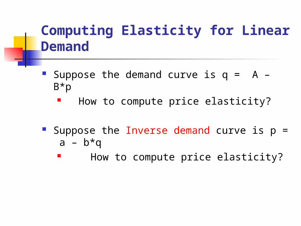
Computing Elasticity for Linear Demand

Suppose the demand curve is q = A – B*p How to compute price elasticity?

Suppose the Inverse demand curve is p = a – b*q How to compute price elasticity?

Solving for Profit-Maximizing Price

Stick with the inverse demand function p = a – b*q Step 1: Increase the quantity produced until the marginal revenue

equals the marginal cost.

Marginal revenue and marginal cost equates at the optimal quantity

2Rev ( )p q a bq q aq bq

Marginal Rev 2a bq *q

*2a bq c *

2

a cq

b

Marginal Cost c

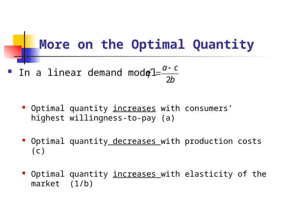
More on the Optimal Quantity

In a linear demand model

Optimal quantity increases with consumers’ highest willingness-to-pay (a)

Optimal quantity decreases with production costs (c)

Optimal quantity increases with elasticity of the market (1/b)

*

2

a cq

b

Solving for Profit-Maximizing Price

Step 2: Compute the optimal price by substituting into the inverse demand function

* *

p a bq

p a bq

*

2

a cq

b

*

2

a cp

More on the Optimal Price

In a linear demand model

Optimal price increases with consumers’ highest willingness-to-pay (a)

Optimal price increases with production costs (c)

Optimal quantity is not affected by the elasticity of the market (1/b)

*

2

a cp

Solving for Profit-Maximizing Price

Step 3: Compute the optimal profit level

At optimum,

Maximal profit is:

Total Profit ( )p c q F

*

2

a cp

*

2

a cq

b

* *

2

( )

( )2 2

( )

4

p c q F

a c a cc F

b

a cF

b

More on the Optimal Profit

In a linear demand model optimal profit is

Optimal profit increases with consumers’ highest willingness-to-pay (a)

Optimal profit decreases with production costs (c)

Optimal profit is increases with the elasticity of the market (1/b)

2( )

4

a c

b

Role of Fixed Cost

Denote fixed cost by F

Decision Rule when Fixed cost has not been incurred Invest if the optimal profit > F Do not invest if the optimal profit < F

Decision Rule when Fixed has already been incurred Invest if the optimal profit > 0

Market Selection

A Firm usually can choose to which market to enter.

Each market will have different fixed costs and demand curve.

Market entry decision depends on the optimal profits of both markets.

Market Selection: An Example

Consider two markets described by the inverse demand functions: p1 = 100 – 0.5*q1 and P2 = 50 – 0.1*q2

The market-specific fixed cost associated with operating in markets 1 and 2 are F1 = F2 = $500.

Marginal Cost is assumed to be the same at $10

The firm can chooses only one market to serve

Market Selection: An Example

Total Profits at Market #1/ Market #2?

Computation follows the three-step procedure outlined above

Which market should be entered?

Enter Market # 1 if the total profit at Market # 1 is higher Enter Market # 2 if the total profit at Market # 2 is higher Need to also account for the fixed cost when we compute the total profit.

Market Selection: An Example Computing the Expected Profit at Market #1 p1 = 100 – 0.5*q1

Step 1: Increase the quantity produced until the marginal revenue equals the marginal cost.

Step 2: Compute the optimal price by substituting into the inverse demand function

Step 3: Compute the optimal profit level

*1

100 1090

2*0.5q

*1

100 10$55

2p

2*1

(100 10)$3550

4 0.5F

Market Selection: An Example Computing the Expected Profit at Market #2 p2 = 50 – 0.1*q2

Step 1: Increase the quantity produced until the marginal revenue equals the marginal cost.

Step 2: Compute the optimal price by substituting into the inverse demand function

Step 3: Compute the optimal profit level

Practice

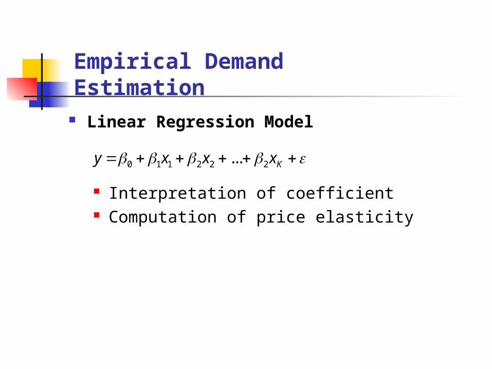
Linear Regression Model

Interpretation of coefficient Computation of price elasticity

Empirical Demand Estimation

0 1 1 2 2 2... Ky x x x

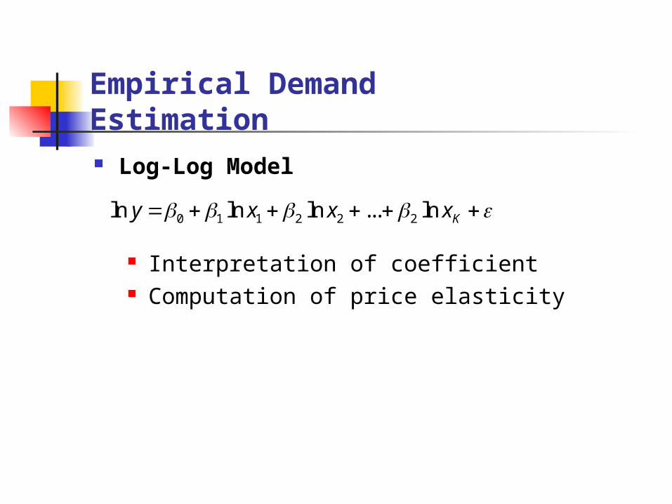
Log-Log Model

Interpretation of coefficient Computation of price elasticity

Empirical Demand Estimation

0 1 1 2 2 2ln ln ln ... ln Ky x x x

Demand Estimation Excel Worksheet

Empirical Demand Estimation - Illustration

Next Lecture

Price Discrimination I