REVENUE MANAGEMENT BEYOND “ESTIMATE, THEN...
113
REVENUE MANAGEMENT BEYOND “ESTIMATE, THEN OPTIMIZE” A DISSERTATION SUBMITTED TO THE DEPARTMENT OF ELECTRICAL ENGINEERING AND THE COMMITTEE ON GRADUATE STUDIES OF STANFORD UNIVERSITY IN PARTIAL FULFILLMENT OF THE REQUIREMENTS FOR THE DEGREE OF DOCTOR OF PHILOSOPHY Vivek Francis Farias June 2007
Transcript of REVENUE MANAGEMENT BEYOND “ESTIMATE, THEN...

REVENUE MANAGEMENT BEYOND
“ESTIMATE, THEN OPTIMIZE”
A DISSERTATION
SUBMITTED TO THE DEPARTMENT OF
ELECTRICAL ENGINEERING
AND THE COMMITTEE ON GRADUATE STUDIES
OF STANFORD UNIVERSITY
IN PARTIAL FULFILLMENT OF THE REQUIREMENTS
FOR THE DEGREE OF
DOCTOR OF PHILOSOPHY
Vivek Francis Farias
June 2007

c© Copyright by Vivek Francis Farias 2007
All Rights Reserved
ii
I certify that I have read this dissertation and that, in my opinion, it is fully
adequate in scope and quality as a dissertation for the degree of Doctor of
Philosophy.
(Benjamin Van Roy) Principal Adviser
I certify that I have read this dissertation and that, in my opinion, it is fully
adequate in scope and quality as a dissertation for the degree of Doctor of
Philosophy.
(Balaji Prabhakar)
I certify that I have read this dissertation and that, in my opinion, it is fully
adequate in scope and quality as a dissertation for the degree of Doctor of
Philosophy.
(Ramesh Johari (Management Science and Engineering))
Approved for the University Committee on Graduate Studies.
iii

iv

Abstract
Modern revenue management systems enable firms to make sophisticated pricing deci-
sions over the course of a sales season. Many of these systems operate within what one
might refer to as the “estimate, then optimize” paradigm where estimation and optimiza-
tion are two distinct, interleaved activities. This thesis will discuss two research efforts
that explore moving away from such a paradigm.
We begin with the study of a simple model of one-resource revenue management
that incorporates uncertainty in demand statistics. The opportunity to learn more about
demand over the course of the sales season introduces a tension between “exploratory”
pricing that attempts to learn quickly and “exploitative” pricing that attempts to exploit
existing demand knowledge so as to maximize revenues. We present a simple heuristic
that addresses this trade-off in a transparent, operationally intuitive, manner. We establish
that pricing decisions that account for this trade-off offer significant increases in revenue
over repeated cycles of “estimate, then optimize.”
We next turn our attention to the dynamic capacity allocation problem that airlines
face. We will present new approximate dynamic programming based algorithms for this
large-scale problem that allow for a seamless integration of complex demand forecast
models within the optimization framework. The algorithms we develop are scalable to
large problems and we present computational results that suggest a significant improve-
ment over methods that rely on frequent re-optimization using a popular linear program-
ming based heuristic.
v

To my parents – Francis and Juliana Farias
vi

Acknowledgements
This thesis is the product of, what for me has been, a very fruitful collaboration with my
advisor and friend Professor Benjamin Van Roy. Ben has taught me the importance of
seeking problems that are of broad interest, formulating them correctly, and not quitting
when the going gets tough. And he has taught me all of this by example, while treating
me no different from a colleague. Life in graduate school can be very trying at times - for
social, academic and other reasons. Ben has, in many ways, displayed a genuine concern
for my well being and this has been as important to me as his guidance in academic
matters. I would be hard-pressed to distinguish my respect for Ben from awe.
Much of the work in this thesis has benefited from the advice of Professor Michael
Harrison, who has always been amazingly accessible. Chapter 2 in this thesis was mo-
tivated by a problem Mike told me about over the course of a Revenue Management
class he taught in 2005 and his emphasis on the importance of moving beyond Poisson
models for Network RM led to Chapter 4 in its current form. I’ve collaborated on other
research problems with Professors Balaji Prabhakar and Tsachy Weissman. I admire
Balaji’s style and his keen knack for formulating elegant problems. The little informa-
tion theory I know, I learned from Tsachy who is in addition to being a gracious teacher,
a formidable problem solver. In recent years I have come to learn some game theory
thanks to Professor Ramesh Johari. We continue to have very stimulating discussions
and although we haven’t written a paper together yet, I hope that changes soon. Finally, I
owe a debt of gratitude to Professor Dunbar Birnie and the late Professor Michael Wein-
berg at the University of Arizona for starting me out with a great deal of care and support
on the path I have chosen.
Graduate school would probably have been very different without my office mate and
vii

good friend, Ciamac Moallemi. Ciamac and I have written two papers together, and I am
certain that our collaboration and friendship will continue over the years to come. Paat
Rusmevichientong and Gabriel Weintraub graciously read parts of this work. They were
also generous with advice for my job search for which I am grateful. I was fortunate to
have as fellow group members David Choi, Jared Han, Kahn Mason, Michael Padilla,
Waraporn Tongprasit and Robbie Yan. The Information Systems Laboratory at Stanford
(ISL) has been a nice place to call home over the last five years – and it wouldn’t be nearly
quite as nice without our administrator Denise Murphy and some of the frighteningly
clever and down-to-earth people I have befriended here.
There are a number of close friends without whose help I wouldn’t have made it this
far in one piece. My good friend Pieter Abbeel has been a sounding board for many ideas
and a constant source of encouragement through times of self doubt. My roommate and
partner-in-crime Jian Wong and I have done a number of things over the last five years
that will hopefully never make it to print – I will really miss those fun times. Among
my other close friends are David Wakayama, Scott Coughlin and Melissa Kar (from my
undergraduate days at Arizona), and Chinmay Belthangady, Ankit Bhagatwala, James
Mammen and Jimmy Zhang here at Stanford. I am grateful to all of them for their
untiring friendship over these years.
My parents Francis and Juliana have over the years sacrificed a great deal to get me
to where I stand today. They are honest and hardworking and I have tried – and will
continue to try – to make myself in their mould. My accomplishments to this point are
primarily the outcome of their parenting. Together with my baby brother Vinay, they are
the people I love the most, and all of this would be hopeless were it not for them.
viii

Contents
Abstract v
Acknowledgements vii
1 Revenue Management Beyond “Estimate, Then Optimize” 1
1.1 What is Revenue Management? . . . . . . . . . . . . . . . . . . . . . 2
1.2 Problems and Models: Two Examples . . . . . . . . . . . . . . . . . . 4
1.3 “Estimate, Then Optimize” . . . . . . . . . . . . . . . . . . . . . . . . 7
1.4 Beyond “Estimate, Then Optimize” . . . . . . . . . . . . . . . . . . . 10
1.5 Further reading . . . . . . . . . . . . . . . . . . . . . . . . . . . . . . 12
2 Dynamic Pricing with an Uncertain Market Response 14
2.1 Introduction . . . . . . . . . . . . . . . . . . . . . . . . . . . . . . . . 15
2.2 Problem Formulation . . . . . . . . . . . . . . . . . . . . . . . . . . . 18
2.3 Optimal Pricing . . . . . . . . . . . . . . . . . . . . . . . . . . . . . . 21
2.3.1 The Case of a Known Arrival Rate . . . . . . . . . . . . . . . . 22
2.3.2 The Case of an Unknown Arrival Rate . . . . . . . . . . . . . . 23
2.4 Estimate, Then Optimize . . . . . . . . . . . . . . . . . . . . . . . . . 24
2.5 The Greedy Heuristic . . . . . . . . . . . . . . . . . . . . . . . . . . . 25
2.6 Decay Balancing . . . . . . . . . . . . . . . . . . . . . . . . . . . . . 26
2.7 Bounds on Performance Loss . . . . . . . . . . . . . . . . . . . . . . . 28
2.7.1 Decay Balancing Versus Optimal Prices . . . . . . . . . . . . . 31
2.7.2 An Upper Bound on Performance Loss . . . . . . . . . . . . . 33
ix

2.7.3 A Uniform Performance Bound for Exponential Reservation
Prices . . . . . . . . . . . . . . . . . . . . . . . . . . . . . . . 35
2.8 Computational Study . . . . . . . . . . . . . . . . . . . . . . . . . . . 37
2.9 Discussion and Conclusions . . . . . . . . . . . . . . . . . . . . . . . 41
3 Decay Balancing Extensions 45
3.1 Multiple Stores and Consumer Segments . . . . . . . . . . . . . . . . . 45
3.2 Product Versioning . . . . . . . . . . . . . . . . . . . . . . . . . . . . 49
3.2.1 Problem Formulation . . . . . . . . . . . . . . . . . . . . . . . 50
3.2.2 Optimal pricing . . . . . . . . . . . . . . . . . . . . . . . . . . 51
3.2.3 Decay Balancing . . . . . . . . . . . . . . . . . . . . . . . . . 52
3.3 Discussion . . . . . . . . . . . . . . . . . . . . . . . . . . . . . . . . . 53
4 Network-RM with Forecast Models 55
4.1 Introduction . . . . . . . . . . . . . . . . . . . . . . . . . . . . . . . . 56
4.2 Model . . . . . . . . . . . . . . . . . . . . . . . . . . . . . . . . . . . 59
4.3 Benchmark Heuristic: The Deterministic LP (DLP) . . . . . . . . . . . 61
4.4 Bid Price Heuristics via Approximate DP . . . . . . . . . . . . . . . . 62
4.4.1 Separable Affine Approximation . . . . . . . . . . . . . . . . . 63
4.4.2 Separable Concave Approximation . . . . . . . . . . . . . . . 64
4.4.3 ALP Solution Properties . . . . . . . . . . . . . . . . . . . . . 65
4.5 Computational Results . . . . . . . . . . . . . . . . . . . . . . . . . . 66
4.5.1 Time homogeneous arrivals (M1) . . . . . . . . . . . . . . . . 68
4.5.2 Multiple demand modes (M2, M3) . . . . . . . . . . . . . . . . 69
4.6 Towards scalability: A simpler ALP . . . . . . . . . . . . . . . . . . . 71
4.6.1 The rALP . . . . . . . . . . . . . . . . . . . . . . . . . . . . . 71
4.6.2 Quality of Approximation . . . . . . . . . . . . . . . . . . . . 74
4.6.3 Computational experience with the rALP . . . . . . . . . . . . 75
4.7 Discussion and Conclusions . . . . . . . . . . . . . . . . . . . . . . . 76
Concluding Remarks 78
x
A Proofs for Chapter 2 79A.1 Proofs of Theorems 1 and 2 . . . . . . . . . . . . . . . . . . . . . . . . 79
A.1.1 Existence of Solutions to the HJB Equation . . . . . . . . . . . 79
A.1.2 Proofs for Theorems 1 and 2 . . . . . . . . . . . . . . . . . . . 83
A.2 Proofs for Section 2.5 . . . . . . . . . . . . . . . . . . . . . . . . . . . 84
A.3 Proofs for Section 2.7 . . . . . . . . . . . . . . . . . . . . . . . . . . . 85
B Proofs for Chapter 4 93B.1 Proofs for Section 4.4 . . . . . . . . . . . . . . . . . . . . . . . . . . . 93
B.2 Proofs for Section 4.6 . . . . . . . . . . . . . . . . . . . . . . . . . . . 95
Bibliography 97
xi

List of Tables
2.1 Decay Balance Price Formulas . . . . . . . . . . . . . . . . . . . . . . 29
2.2 Decay Balance vs. Optimal Prices . . . . . . . . . . . . . . . . . . . . 33
2.3 Performance vs. a Clairvoyant algorithm . . . . . . . . . . . . . . . . . 38
4.1 Solution quality and computation time for the rALP and ALP. * indicates
values for an RLP with 100,000 constraints (recall that the RLP provides
a lower bound on the ALP). ** indicates values for the sampled rALP
described in section 6.3 using the same sample set as that in the compu-
tation of the corresponding RLP. Computation time reported in seconds
for the CPLEX barrier LP optimizer running on a workstation with a 64
bit AMD processor and 8GB of RAM. . . . . . . . . . . . . . . . . . . 76
xii
List of Figures
2.1 Lower bound on Decay Balancing performance . . . . . . . . . . . . . 35
2.2 Decay Balancing price trajectories vs. Clairvoyant price trajectories . . 38
2.3 Performance gain over the Certainty Equivalent and Greedy Pricing heuris-
tics at various inventory levels . . . . . . . . . . . . . . . . . . . . . . 39
2.4 Maximal performance gain over the Certainty Equivalent Heuristic (left)
and Greedy Heuristic (right) for various coefficients of variation . . . . 44
3.1 Performance relative to a clairvoyant algorithm . . . . . . . . . . . . . 48
3.2 Performance relative to the Certainty Equivalent (left) heuristic and Greedy
Pricing heuristic (right) . . . . . . . . . . . . . . . . . . . . . . . . . . 54
4.1 Performance relative to the DLP for model M1 . . . . . . . . . . . . . 66
4.2 Performance relative to the DLP for model M1 . . . . . . . . . . . . . 67
4.3 Performance relative to the DLP for model M2 . . . . . . . . . . . . . 68
4.4 Performance relative to the DLP for model M2 . . . . . . . . . . . . . 69
4.5 Performance relative to the DLP for model M3 . . . . . . . . . . . . . 70
xiii

xiv

Chapter 1
Revenue Management Beyond“Estimate, Then Optimize”
“Revenue Management” (or RM for short) is today a ubiquitous area of operations re-
search that is concerned with developing into a science, the art of selling the right item,
to the right person, at the right price. This thesis is concerned with addressing the flaws
of an operational paradigm we refer to as “estimate, then optimize”, that has become
commonplace in the modern practice of revenue management. Our objective is to pro-
pose new schemes that, by appropriately addressing these flaws, are capable of adding to
the revenues generated by existing RM mechanisms.
This chapter begins with a brief introduction to the field of revenue management.
We then introduce the “estimate, then optimize” paradigm in the context of two fairly
commonplace RM models. After a discussion of the flaws inherent to this paradigm,
we provide a brief overview of the contributions made by this thesis in addressing those
flaws. We restrict ourselves in this chapter to a high level, qualitative discussion; sub-
sequent chapters will make more detailed arguments supported either by mathematical
results or computational evidence.
1

2 CHAPTER 1. BEYOND “ESTIMATE, THEN OPTIMIZE”
1.1 What is Revenue Management?
Revenue management has over the years come to be associated with a broad variety of
sales practices across an equally broad array of industries. It is therefore natural that
any attempt at a concise description of the term is likely to fail to capture the finer nu-
ances of the practice. Nonetheless, we attempt to provide such a description: Revenue
management refers to the optimal or near-optimal use of a sales mechanism so as to
maximize over some period, expected revenues from the sale of one or more products,
each requiring quantities of one or more potentially scarce resources. While certainly
not comprehensive, this definition is rather broad. In particular, the products in question
could be essentially anything ranging from airline tickets, hotel rooms and fashion goods
on the one hand, to power and natural gas on the other. The sales mechanisms employed
could also vary widely. For example, a product may be sold at a posted price in which
case the seller must decide on what prices to post over time. As another example, items
of a product may be auctioned in which case the seller must design a suitable auction
mechanism. Finally, the phrases “optimal use” and “maximize expected revenues” sug-
gest a well specified mathematical optimization problem and a number of reasonable
formulations are likely to be viable for a given revenue management problem. The very
act of selling a product entails making the types of decisions we have alluded to and it is
this last feature – the mathematical systematization of the typical decisions that must be
made by a seller – that distinguishes RM.
To get a sense for the diversity inherent to the practice of RM, consider the following
instances: Airlines offer an array of “fare-products” (which are essentially itinerary-
price-restriction combinations) whose availability are carefully modulated over time us-
ing RM tools. Potential customers arrive through varied sources such as internet travel
sites or through a travel agent which in turn, through an interface with the airline’s reser-
vation management system, allow the customer to choose from fare-products that are
available at that point in time. Fashion goods are typically sold through retail outlets
where prices posted for various items are adjusted multiple times over the course of a
sales season based on a multitude of factors including the perceived popularity of the
item and its availability. Again such price adjustments often require the support of an

1.1. WHAT IS REVENUE MANAGEMENT? 3
RM system. As yet another example, Natural gas pipeline operators offer a variety of
gas delivery contracts at rates that depend on available capacity on their pipelines and gas
futures prices in spot markets (such as the New York Mercantile Exchange); customers
are typically utility companies or large industrial units and purchases may be made either
directly or through online market places such as the Intercontinental Exchange. Again,
RM systems aid managers in pricing such products.
Effective RM tools can have an enormous impact on the revenues and profits of a
firm. While there is no dearth of examples across industries, one of the most notable,
and perhaps earliest, success stories is the American Airlines RM system “DINAMO”.
By carefully controlling the availability of various fare-products on their network via
DINAMO, American estimates that they added 1.4 Billion dollars to their bottom line
for the period from 1989-92 (see Smith et al. (1992)). This level of success, however,
is contingent upon a number of factors. These include: engineering an information pro-
cessing system that streamlines the sales process and the acquisition of sales data that
a manager might find useful, building mathematical models that capture features of the
sales process that managers believe to be important, and finally the design of algorithmic
tools to support decision making within these models. There are two broad classes of
algorithmic problems that arise in this context:
Forecasting and Estimation: A “forecast model” is a black box that predicts demand
for products based on factors such as price, popularity and historical demand for that
product and similar products, market factors such as competitor prices and so forth.
Firms treat their proprietary forecast models as trade secrets. Designing good forecast
models is an art and typically requires an experts intuition. Using a forecast model typi-
cally requires some manner of statistical estimation – be it regressions against historical
data to estimate forecast model parameters, or Bayesian updating to estimate state in
a state-space model of demand. As such the design of forecast models and estimators
leverages a number of tools from the statistics and econometrics literature.
Optimization: Many revenue management problems are posed as optimization prob-
lems; inventory constraints and uncertainty in demand make these problems stochastic
and dynamic. These optimization problems are often computationally difficult, the chief
difficulty arising from having to jointly manage inventory levels of multiple resources

4 CHAPTER 1. BEYOND “ESTIMATE, THEN OPTIMIZE”
and from the complexities of the processes that describe demand. Optimal solution is
rarely possible, and heuristics that relax inventory constraints in certain ways or that
make simplifying assumptions about demand are often called for.
This thesis is concerned with issues that arise in the design of optimization tools for
an RM system. We next introduce two problems that arise in the context of retail and
airline RM respectively. These will serve as illustrative examples for our discussion over
the remainder of this chapter.
1.2 Problems and Models: Two Examples
Example 1. Dynamic Pricing for a Single Product
Consider a retailer selling a single product over some finite sales season. At every
point in time, the retailer must post a price should he have inventory of the product on
hand. An arriving customer must pay the posted price at that time should he choose to
acquire the product. In building an RM system to decide what price to post at each point
in time, the retailer might begin with the following modeling assumptions:
1. Potential customers arrive according to some stochastic point process (say a Pois-
son process).
2. Arriving customers have “reservation prices” and make a purchase if and only if
their reservation price exceeds the posted price.
3. Reservation prices are themselves random and distributed according to some known
distribution.
With these three modeling assumptions, and assuming the retailer has succeeded in es-
timating the rate at which customers arrive and their reservation price distribution, one
may show that his optimal pricing decision is a function of the time remaining in the
sales season and the inventory he has on hand. Dynamic programming may then be used
to compute the optimal price function.
Example 2. Capacity Control for Airline Network RM

1.2. PROBLEMS AND MODELS: TWO EXAMPLES 5
Consider an airline that operates flights across a network of cities. The airline sells
fare-products, a given fare-product being completely specified by its associated itinerary,
price and restrictions (such as the non-refundability of a canceled ticket). In selling
tickets for flights on a particular date in the future, the airline must at suitably frequent
intervals of time up to that date decide which fare-products it will make available until
the next decision epoch. Of course, the airline can make available a given fare-product
only if it has seats available on the flight legs required for that product 1. An arriving
customer may be interested in a subset of fare-products offered by the airline and must
choose among available products (or not purchasing). Again, the retailer might begin
with a few modeling assumptions:
1. Arriving customers have reservation prices for each of the products available upon
their arrival and choose to purchase the product that maximizes their surplus (that
is, the difference between their reservation price for the product and its price). A
customer buys nothing if no product offers him a positive surplus.
2. Customer reservation prices for the products offered are themselves random and
jointly distributed according to some known distribution; there are several cus-
tomer “types” – each type is associated with a specific joint distribution of reser-
vation prices.
3. Potential customers of each type arrive according to some stochastic point process
(such as a Poisson process) specific to that type.
Again, assuming that the revenue manager is able to estimate the required arrival rates
and reservation price distributions, the optimal capacity allocation decision at every
point in time may be shown to be a function of available capacities on each network leg
and the time remaining to the end of the sales horizon. The optimal capacity allocation
function may be found via dynamic programming, though the compute time required
would likely render such an approach impractical.
A seller is ultimately interested in the net proceeds from all sales over the course of
a sales season and the sales mechanisms implicit in Examples 1 and 2 are by no means1Although, in general one may also consider over-booking

6 CHAPTER 1. BEYOND “ESTIMATE, THEN OPTIMIZE”
the only – or most suitable – mechanisms possible. For example, the retailer may choose
to sell products via a dynamic auction of some sort. In the case of airline network ca-
pacity allocation the notion of a fare-product is somewhat synthetic – at the very least it
imposes an unnecessary discretization on the price a consumer is charged. Deciding on
the “right” sales mechanism, while important, depends on a large number of factors in-
cluding laws (such as those forbidding price discrimination) or the infrastructure in place
to support the sales mechanism (such as the computer reservation processing system an
airline might have in place). As such, many industries including the airline and fashion
retail industries have established sales mechanisms in place that have seen few, if any,
fundamental changes in decades. We will, in problems we consider in this thesis, not
consider these issues and instead treat the sales mechanism as a given.
Example 1 outlines a potential RM system for the retailer’s problem. Its success
hinges on the validity of the modeling assumptions and the ability of the retailer to es-
timate customer arrival rate and the reservation price distribution. Having done so, the
relevant dynamic program is in fact quite simple. Even so, it is unlikely that accurate
estimates of the type needed are available at the start of a sales season, and in practice
these estimates might be refined as the sales season unfolds.
The network capacity control problem is more complex. For one, even if the mod-
eler were able to identify customer types, it is unlikely that sufficient data for reliable
estimates of joint reservation price distributions for each of these types will be avail-
able. Even if these difficulties could somehow be surmounted, the relevant dynamic
optimization problem that one must solve to compute optimal capacity allocation deci-
sions suffers from the “curse of dimensionality” and is, for all practical purposes, not
amenable to efficient solution. This necessitates the consideration of further specialized
models. For example, one may restrict attention to parametric families of reservation
price distributions. Assuming that the data to estimate such a model is available one is
still left with a difficult dynamic optimization problem. A natural simplification is to
assume customer arrival processes are deterministic with rates that agree with observed
averages. In doing so, we are left with a far simpler, often tractable, optimization prob-
lem. While such simplifications yield tractability, it is clear that models of this nature
are likely to provide very crude descriptions of demand and not leverage the full power
1.3. “ESTIMATE, THEN OPTIMIZE” 7
of a good forecast model’s abilities. Coping with these difficulties is something of an
art, but typical strategies include repeated model re-estimation and optimization of the
re-estimated model.
1.3 “Estimate, Then Optimize”
Consider a vendor of Winter apparel. New items are stocked in the Autumn and sold over
several months. Because of significant manufacturing lead times and fixed costs, items
are not restocked over this period. Evolving fashion trends generate great uncertainty in
the number of customers who will consider purchasing these items. To optimize revenue,
the vendor should adjust prices over time. But how should these prices be set as time
passes and units are sold? At first sight, this problem appears amenable to the type of
modeling that Example 1 suggests. A problematic issue however, is that at the start of the
sales season, the retailer is unlikely to have reliable estimates of the customer arrival rate
or perhaps even the reservation price distribution required for that model. How might
one address this issue?
One pragmatic solution proceeds as follows: Start with a guess for the customer
arrival rate and reservation price distribution. There are many reasonable ways of coming
up with a good guess. For example, market research or historical sales data for similar
products that were sold in the past might be used to estimate these quantities. Given such
a guess, solve the necessary dynamic optimization problem to compute an optimal price
(assuming the guess is correct). As the sales season unfolds, the retailer accumulates new
data on the frequency with which he sees customers purchasing his product at various
price levels which in turn allows him to refine his guess of arrival rate and reservation
price distribution. He then solves a new dynamic optimization problem based on these
revised estimates and proceeds to price based on the solution to this new problem. A
procedure of this type could potentially be repeated many times over the course of a
sales season with estimates that improve over time. For obvious reasons, we refer to this
as the “estimate, then optimize” paradigm.
There are some qualitative differences in the nature of the demand uncertainties faced
8 CHAPTER 1. BEYOND “ESTIMATE, THEN OPTIMIZE”
by a fashion retailer and an airline revenue manger. In particular, the airline is in a posi-
tion to produce more accurate demand forecasts. For instance, the airline will have ac-
cess to large quantities of historical data that let the airline calibrate complex forecasting
models. Such models might be capable of predicting demand contingent on historical
information and various other relevant factors. One mathematical abstraction for such
a forecasting model is a Markov-modulated Poisson process with partially observable
modulating states. The role of estimation here is then to estimate the underlying state in
such a model.
The underlying dynamic optimization problem for the capacity allocation problem
is challenging even in the context of simple stochastic demand processes (such as time
homogeneous Poisson processes). As such, it is not uncommon in formulating an opti-
mization problem, to assume that demand for a given fare product is deterministic and
equal to the expected forecasted demand, and make allocation decisions based on such an
assumption. The revenue manager then relies on frequently updating the demand quanti-
ties assumed by the optimization algorithm in the hope that this corrects for the fact that
the algorithm assumes a model that is a poor description of reality although this clearly
fails to utilize all of the forecasting models potential predictive abilities. Although more
complex, the “estimate, then optimize” cycle in the case of network capacity control con-
tinues to fulfill the same two basic needs as it did in the case of the retailers problem: one
is the need to compute updated forecasts, and the second is to update the optimization
model inputs so as to compensate for the fact that it assumes a crude model for demand.
The “estimate, then optimize” paradigm is a natural means to addressing the com-
plexities inherent to revenue management in the face of large uncertainties in demand.
But it is not without its flaws:
1. Optimizing assuming the “wrong” model of demand: For an optimization al-
gorithm to use a cruder model of customer demand than is available is an obvious
shortcoming. Over each optimization phase, the retailer assumes that demand is a
Poisson process of a deterministically known rate, whereas in reality there is un-
certainty in this rate which is unaccounted for; depending on the precise nature of
this uncertainty, the retailer may want to adjust prices so as to hedge effectively
1.3. “ESTIMATE, THEN OPTIMIZE” 9
against the possibilities of a favorable or unfavorable demand environment. Simi-
lar problems are evident with using a crude demand model in the network capacity
control case. In particular, consider the following toy forecast model: the model
predicts constant demand up to a certain point in time. Beyond that point, demand
either goes up by 20 % or falls by 20 % with equal probability. Under the “esti-
mate, then optimize” paradigm, an optimization algorithm that operates based on
expected demand forecasts will assume that demand is to remain constant over all
time, and updates this assumption only once demand actually does change. Such
an algorithm cannot be expected to hedge effectively between the two potential
outcomes of demand going up by 20 % or falling by 20 %.
2. Ignoring the incentive to learn: The price set by the fashion retailer impacts,
in addition to his revenues, the rate at which he is able to learn about customer
demand. In particular, price serves to censor demand, so that at high prices the
retailer learns slowly thereby potentially wasting precious selling time, whereas at
low prices he learns quickly but at the expensive of potentially precious inventory.
Clearly a trade-off needs to be made between eliminating uncertainty in demand
statistics, exploiting existing demand knowledge and hedging against the possi-
bility that demand for the product is in fact higher than expected. The “estimate,
then optimize” paradigm ignores these trade-offs entirely. The same criticism is
relevant to the case of network capacity control as well. In particular, the relevant
inputs to a forecast model for network capacity control need to be estimated. For
example, in the case of Markov-modulated demand with partial observability, the
underlying arrival rate modulating state needs to be estimated. A high degree of
uncertainty in the underlying state might call for controls that quickly eliminate
this uncertainty so as to have accurate forecasts available.
These flaws are by no means subtle. We are naturally led to wonder:
• Would addressing these issues produce a tangible impact on revenues?
• Can these flaws be addressed in a manner that is robust and efficient?
Our intention is to explore these questions.

10 CHAPTER 1. BEYOND “ESTIMATE, THEN OPTIMIZE”
1.4 Beyond “Estimate, Then Optimize”
This thesis makes an attempt to move beyond the “estimate, then optimize” paradigm
and address some of its flaws. The paradigm – like our discussion thus far – is quite
general and making progress requires us to specialize our attention in several ways. For
one, formulating well posed problems will require us to restrict focus to specific revenue
management models. We focus in turn on two models very similar in spirit to those
suggested in Examples 1 and 2. Both models we consider are natural generalizations of
optimization models commonplace in the academic RM literature. The generalizations
we incorporate allow for richer forms of demand uncertainty and capture features of real
world problems that we believe are generally ignored in the formulation of RM optimiza-
tion problems for want of tractable solution techniques; they are instead typically dealt
with via repeated iterations of estimation followed by re-optimization.
We consider in Chapter 2, a model for one product dynamic pricing where we in-
corporate uncertainty in demand via the introduction of a prior on customer arrival rate;
such models typically call for the solution of high dimensional dynamic programming
problems and standard models typically ignore this type of uncertainty. In addition to
having several potential real-world applications, our model allows us to understand in a
precise way some of the flaws inherent to a scheme based on “estimate, then optimize”.
Chapter 2 makes several contributions. Among them:
• We propose “decay balancing” – a simple, new heuristic for dynamic pricing in the
face of demand uncertainty. Unlike methods that rely on repeated re-optimization
based on revised estimates of expected arrival rate, decay balancing prices implic-
itly account for the level of uncertainty in making pricing decisions. While being
no more complex than a typical “estimate, then optimize” type scheme, decay bal-
ancing shows performance improvements of up to about 30% over such schemes.
• We demonstrate performance guarantees for our heuristic, including a uniform
performance bound: For Gamma priors on arrival rates and exponential reserva-
tion prices, Decay balancing is a 3-approximation algorithm. Such bounds are
indicators of robustness across all parameter regimes; computationally observed
performance losses are on the order of 1-2%.

1.4. BEYOND “ESTIMATE, THEN OPTIMIZE” 11
• We derive key structural properties that an optimal scheme must possess and show
that Decay Balancing inherits these properties.
In the previous section, we were led to ask whether overcoming the flaws inherent
to the “estimate, then optimize” paradigm could have a tangible impact on revenues,
and whether this could be accomplished via simple schemes. For the one product RM
model introduced in Chapter 2, decay balancing provides an affirmative answer to both
questions.
Chapter 4 considers a model for network RM wherein customers arrive according
to a Markov modulated Poisson process. This is a substantial generalization of the de-
terministic rate customer arrival processes considered in a majority of the network RM
literature. It is an important generalization since it allows for the integration of relatively
complex demand forecast models in the optimization process. One might hope that op-
timal or near optimal solutions to dynamic optimization problems that arise from such
models would lead to improvements over schemes that rely on solutions to optimization
problems that assume far cruder models of demand (such as expected demand forecasts).
Solving such optimization problems however is non-trivial, and Chapter 4 makes several
contributions in this direction:
• We develop an approximation algorithm for a dynamic capacity allocation problem
arising from a network RM model with Markov modulated arrival rates. Our algo-
rithm is based on the linear programming (LP) approach to approximate dynamic
programming (DP).
• Our algorithm demonstrates performance gains of up to 8% over an approach that
uses only expected demand forecasts. The approach we compare our performance
to is representative of the state of the art in network RM optimization.
• Our algorithm is scalable. In particular, its use requires the one time solution of a
single LP that even for large networks could potentially be solved in minutes.
Chapter 4 proposes models and algorithms with a view to allowing for more realistic
demand modeling in optimization for network RM. The results in that chapter suggest

12 CHAPTER 1. BEYOND “ESTIMATE, THEN OPTIMIZE”
that doing so is likely to be viable in practice and could in addition to yielding levels
of performance superior to the state of the art, substantially reduce dependence on the
frequent re-optimization necessary for optimization models that assume crude models of
demand.
The “estimate, then optimize” paradigm is applicable to a number of models beyond
the scope of this thesis and is an approach that is easily understood and adapted. The
schemes we propose on the other hand, while relatively simple to implement, are tai-
lored to specific models. The decay balancing heuristic can be extended to models other
than the vanilla one-product dynamic pricing problem in Chapter 2 (see Chapter 3), and
the approximate DP approach that drives the algorithms in Chapter 4 is almost certainly
applicable to many problems in RM that call for the solution of high dimensional dy-
namic programs. Nonetheless, moving beyond the “estimate, then optimize” paradigm
in general is likely to require some effort on the part of the algorithm designer. In a world
where 1-2% gains in revenue have potentially large implications for the profits of a firm,
this effort is likely to be well rewarded.
1.5 Further reading
Revenue management is a fairly broad area of research and borrows heavily from fields
such as marketing, statistics and stochastic control. The books by Talluri and van Ryzin
(2004) and Phillips (2005) are excellent, encyclopedic resources for a broad overview
of the area. Little is available in the way of literature on the estimation and forecasting
practices in the RM industry, and these texts are among the few thorough treatments of
those areas. In contrast, much of the academic RM literature is dedicated to optimization
problems that arise in various RM contexts.
There are a number of papers on various aspect of airline RM. Smith et al. (1992)
provides an overview of the RM heuristics that went into building American Airlines’
first successful RM system DINAMO while P.P.Belobaba (2001) surveys industry prac-
tice. Papers by Gallego and van Ryzin (1997), Bertsimas and de Boer (2005), van Ryzin
and McGill (2000) and Bertsimas and Popescu (2003) are representative of modern al-
gorithmic approaches to the network RM dynamic capacity allocation problem. The

1.5. FURTHER READING 13
main thrust of the work in these papers is designing effective means of dealing with the
curse of dimensionality that arises from having to jointly manage multiple resources in
network RM problems. RM for the natural gas and fashion industries are of relatively
newer vintage; as examples, Talluri and van Ryzin (2004) discuss RM problems that
arise in the natural gas industry while Bitran and Mondschein (1997) consider optimal
markup/ markdown policies for fashion retail.
Gallego and van Ryzin (1994) undertake a detailed study of a model similar to that
in Example 1 and provide optimal and heuristic dynamic pricing policies under the as-
sumption of known arrival rates and reservation price distributions while a subsequent
paper (Gallego and van Ryzin (1997)) considers the multi-dimensional (that is, multi-
resource, multi-product) generalization to that problem. Alternative sales mechanisms –
such as dynamic auctions – have not been throughly studied in an RM context. Vulcano
et al. (2002) explores the use of a dynamic auction for a one resource, finite time horizon
revenue management problem.
The “estimate, then optimize” paradigm has received little attention in the literature;
an exception is Eren and Maglaras (2006) that points out the potential dangers of using
such an approach for a certain one product RM problem. Other authors have recognized
some of the flaws inherent to the paradigm in the context of problems such as examples
1 and 2 and proposed alternatives; we will discuss that work in subsequent chapters.

Chapter 2
Dynamic Pricing with an UncertainMarket Response
This chapter studies a problem of dynamic pricing faced by a vendor with limited inven-
tory, uncertain about demand, aiming to maximize expected discounted revenue over an
infinite time horizon. The vendor learns from purchase data, so his strategy must take
into account the impact of price on both revenue and future observations; a key flaw
of the “estimate, then optimize” paradigm was its failure to account for this trade-off.
We focus on a model in which customers arrive according to a Poisson process, each
with an independent, identically distributed reservation price. Upon arrival, a customer
purchases a unit of inventory if and only if his reservation price equals or exceeds the
vendor’s prevailing price.
We propose in this chapter a new heuristic approach to pricing, which we refer to as
decay balancing. Among other performance bounds, we establish that when reservations
prices are exponentially distributed and the vendor begins with a Gamma prior over ar-
rival rates, decay balancing always garners at least one-third of the maximum expected
discounted revenue. This is the first heuristic for problems of this type for which a uni-
form performance bound is available. We also establish that changes in inventory and
uncertainty in the arrival rate bear appropriate directional impacts on decay balancing
prices, in contrast to the recently proposed certainty equivalent and greedy heuristics.
Further, we provide computational results to demonstrate that decay balancing offers
14

2.1. INTRODUCTION 15
significant revenue gains over these alternatives. The decay balancing heuristic may be
extended to several interesting related models; we pursue these extensions in the next
chapter.
The remainder of this chapter is organized as follows: Section 2.1 introduces the
problem and places it in the context of other work in the general area of pricing in the
face of demand uncertainty. In Section 2.2, we formulate our model and cast our pricing
problem as one of stochastic optimal control. Section 2.3 develops the HJB equation
for the optimal pricing problem in the contexts of known and unknown arrival rates.
Section 2.4 introduces an existing “estimate, then optimize” style heuristic (the certainty
equivalent heuristic) for the problem, while section 2.5 introduces a recently proposed
heuristic that attempts to address the flaws inherent to an “estimate, then optimize” based
approach. Section 2.6 introduces decay balancing which is the focus of this chapter. This
section also discusses structural properties of the decay balancing policy. Section 2.7 is
devoted to a performance analysis of the decay balancing heuristic. When the arrival
rate is Gamma distributed and reservation prices are exponentially distributed, we prove
a uniform performance guarantee for our heuristic. Section 2.8 presents a computational
study that compares decay balancing to certainty equivalent and greedy pricing heuristics
as well as a clairvoyant algorithm. Finally, in Section 2.9 we conclude with thoughts on
future prospects for this work.
2.1 Introduction
In motivating the need to consider moving beyond the “estimate, then optimize” paradigm,
the last chapter considered the example of a vendor of winter apparel who needed to ad-
just prices over time in the face of limited inventory and great uncertainty in the number
of customers who might consider purchasing his product. This is representative of prob-
lems faced by many vendors of seasonal, fashion, and perishable goods.
There is a substantial literature on pricing strategies for such a vendor (see Talluri
and van Ryzin (2004) and references therein). Gallego and van Ryzin (1994), in par-
ticular, formulated an elegant model in which the vendor starts with a finite number of
identical indivisible units of inventory. Customers arrive according to a Poisson process,

16 CHAPTER 2. UNCERTAIN MARKET RESPONSE
with independent, identically distributed reservation prices. In the case of exponentially
distributed reservation prices the optimal pricing strategy is easily derived. The analysis
of Gallego and van Ryzin (1994) can be used to derive pricing strategies that optimize
expected revenue over a finite horizon and is easily extended to the optimization of dis-
counted expected revenue over an infinite horizon. Resulting strategies provide insight
into how prices should depend on the arrival rate, expected reservation price, and the
length of the horizon or discount rate.
Our focus in this chapter is on an extension of this model in which the arrival rate
is uncertain and the vendor learns from sales data. Incorporating such uncertainty is un-
doubtedly important in many industries that practice revenue management. For instance,
in the Winter fashion apparel example, there may be great uncertainty in how the market
will respond to the product at the beginning of a sales season; the vendor must take into
account how price influences both revenue and future observations from which he can
learn.
In this setting, it is important to understand how uncertainty should influence price.
However, uncertainty in the arrival rate makes the analysis challenging. Optimal pricing
strategies can be characterized by a Hamilton-Jacobi-Bellman (HJB) Equation, but there
is no known analytical solution. Further, for arrival rate distributions of interest, grid-
based numerical methods require discommoding computational resources and generate
strategies that are difficult to interpret. As such researchers have designed and analyzed
heuristic approaches.
Aviv and Pazgal (2005) studied a certainty equivalent heuristic for exponentially dis-
tributed reservation prices which at each point in time computes the conditional expec-
tation of the arrival rate, conditioned on observed sales data, and prices as though the
arrival rate is equal to this expectation. This is precisely the “estimate, then optimize”
paradigm and it inherits the flaws of that paradigm we pointed out in the introductory
chapter. In particular, it uses an incorrect demand model and further ignores the incen-
tive to learn.
In an effort to address these flaws Araman and Caldentey (2005) recently proposed a
more sophisticated heuristic that takes arrival rate uncertainty into account when pricing.
The idea is to use a strategy that is greedy with respect to a particular approximate value

2.1. INTRODUCTION 17
function. In this chapter, we propose and analyze decay balancing, a new heuristic ap-
proach which makes use of the same approximate value function as the greedy approach
of Araman and Caldentey (2005).
Several idiosyncrasies distinguish the models studied in Aviv and Pazgal (2005) and
Araman and Caldentey (2005). The former models uncertainty in the arrival rate in
terms of a Gamma distribution, whereas the latter uses a two-point distribution. The
former considers maximization of expected revenue over a finite horizon, whereas the
latter considers expected discounted revenue over an infinite horizon. To elucidate rela-
tionships among the three heuristic strategies, we study them in the context of a common
model. In particular, we take the arrival rate to be distributed according to a finite mixture
of Gamma distributions. This is a very general class of priors and can closely approx-
imate any bounded continuous density. We take the objective to be maximization of
expected discounted revenue over an infinite horizon. It is worth noting that in the case
of exponentially distributed reservation prices such a model is equivalent to one with-
out discounting but where expected reservation prices diminish exponentially over time.
This may make it an appropriate model for certain seasonal, fashion, or perishable prod-
ucts. Our modeling choices were made to provide a simple, yet fairly general context for
our study. We expect that our results can be extended to other classes of models such as
those with finite time horizons, though this is left for future work.
When customer reservation prices are exponential and the arrival rate is Gamma dis-
tributed we prove that decay balancing always garners at least 33.3% of the maximum
expected discounted revenue. Allowing for a dependance on the number of sales we can
show that after four sales decay balancing achieves at least 80% of optimal performance
thereafter. It is worth noting that no performance loss bounds (uniform or otherwise)
have been established for the certainty equivalent and greedy approaches. Further, our
computational results suggest that our theoretical bounds are conservative and also that
decay balancing offers substantial increases in revenue relative to certainty equivalent
and greedy approaches. Surprisingly, though the two heuristics are based on the same
approximate value function, switching from the greedy approach to decay balancing can
increase expected discounted revenue by over a factor of three. Further, uncertainty in
the arrival rate and changes in inventory bear appropriate directional impacts on decay

18 CHAPTER 2. UNCERTAIN MARKET RESPONSE
balancing prices: uncertainty in the arrival rate increases price, while a decrease in inven-
tory increases price. In contrast, uncertainty in the arrival rate has no impact on certainty
equivalent prices while greedy prices can increase or decrease with inventory.
Aside from Aviv and Pazgal (2005) and Araman and Caldentey (2005), there is a sig-
nificant literature on dynamic pricing while learning about demand. Lin (2007) considers
a model identical to Aviv and Pazgal (2005) and develops heuristics which are motivated
by the behavior of a seller who knows the arrival rate and anticipates all arriving cus-
tomers. Bertsimas and Perakis (2003) develop several algorithms for a discrete, finite
time-horizon problem where demand is an unknown linear function of price plus Gaus-
sian noise. This allows for least-squares based estimation. Lobo and Boyd (2003) study
a model similar to Bertsimas and Perakis (2003) and propose a “price-dithering” heuris-
tic that involves the solution of a semi-definite convex program. All of the aforemen-
tioned work is experimental; no performance guarantees are provided for the heuristics
proposed. Cope (2006) studies a Bayesian approach to pricing where inventory levels
are unimportant (this is motivated by sales of on-line services) and there is uncertainty
in the distribution of reservation price. His work uses a very general prior distribution
(a Dirichlet mixture) on reservation price. Modeling this type of uncertainty within a
framework where inventory levels do matter represents an interesting direction for future
work. In contrast with the the above work, Burnetas and Smith (1998) and Kleinberg
and Leighton (2004) consider non-parametric approaches to pricing with uncertainty in
demand. However, those models again do not account for inventory levels. Recently,
Besbes and Zeevi (2006) presented a non-parametric algorithm for ”blind“ pricing; they
present a pricing algorithm for pricing multiple products that use multiple resources, sim-
ilar to the model considered in Gallego and van Ryzin (1997). Their algorithm requires
essentially no knowledge of the demand function. While the algorithm is optimal under a
certain fluid-limit like scaling, the algorithm requires testing every possible price vector
within a multidimensional grid which represents a discretization of the space of price
vectors.

2.2. PROBLEM FORMULATION 19
2.2 Problem Formulation
We consider a problem faced by a vendor who begins with x0 identical indivisible units
of a product and dynamically adjusts price pt over time t ∈ [0,∞). Customers arrive
according to a Poisson process with rate λ. As a convention, we will assume that the
arrival process is right continuous with left limits. Each customer’s reservation price is an
independent random variable with cumulative distribution F (·). A customer purchases a
unit of the product if it is available at the time of his arrival at a price no greater than his
reservation price; otherwise, the customer permanently leaves the system.
For convenience, we introduce the notation F (p) = 1− F (p) for the tail probability.
We place the following restrictions on F (·):
Assumption 1.
1. F (·) has a density f(·) with support R+.
2. ρ(p)
F (p)is an increasing function of p, where ρ(p) = f(p)
F (p)is the hazard rate function
for F .
3. p− 1/ρ(p) is a surjective function of p with R+ in it’s range.
The first assumption is a regularity assumption. Now, one may think of F (p) ≡ q
as the expected quantity of the product sold at price p garnering the seller an expected
revenue of R(p) = pF (p). By the first part of Assumption 1, given a quantity q ∈ (0, 1],
the unique price that achieves this expected quantity is given by p(q) = F−1(1 − q),
so that expected revenue can also be thought of as a function of q, R(q) = R(p(q)).
The marginal revenue to the seller with respect to quantity is then given by dR/dq =
p(q) − 1/ρ(p(q)). S. Ziya and Foley (2004) note that if f is differentiable, the second
assumption is equivalent to the statement that marginal revenue with respect to quantity
is increasing in price and equivalently, decreasing in quantity. This is a reasonable eco-
nomic premise. If the first and second parts of Assumption 1 hold, the assumption that
p − 1/ρ(p) is surjective with range R+ is equivalent to assuming that expected revenue
in the presence of a finite non-negative marginal cost c, (p − c)F (p), is maximized at
some finite price p∗. This too appears to be reasonable. Our assumptions are standard

20 CHAPTER 2. UNCERTAIN MARKET RESPONSE
to the revenue management literature (see Talluri and van Ryzin (2004) pp. 315-318)
and permit us to use first order optimality conditions to characterize solutions to various
optimization problems that will arise in our discussion.
Let tk denote the time of the kth purchase and nt = |{tk : tk ≤ t}| denote the number
of purchases made by customers arriving at or before time t. The vendor’s expected
revenue, discounted at a rate of α > 0, is given by
E
[∫ ∞
t=0
e−αtptdnt
].
Let τ0 = inf{t : xt = 0} be the time at which the final unit of inventory is sold. For
t ≤ τ0, nt follows a Poisson process with intensity λF (pt). Consequently, one may show
that
E
[∫ ∞
t=0
e−αtptdnt
]= E
[∫ τ0
t=0
e−αtptλF (pt)dt
].
We now describe the vendor’s optimization problem. Because of differences in these
two contexts, we first consider the case where the vendor knows λ and later allow for
arrival rate uncertainty. In the case with known arrival rate, we consider pricing policies
π that are measurable real-valued functions of the inventory level. The price is irrelevant
when there is no inventory, and as a convention, we will require that π(0) = ∞. We
denote the set of policies by Πλ. A vendor who employs pricing policy π ∈ Πλ sets price
according to pt = π(xt), where xt = x0 − nt, and receives expected discounted revenue
Jπλ (x) = Ex,π
[∫ τ0
t=0
e−αtptλF (pt)dt
],
where the subscripts of the expectation indicate that x0 = x and pt = π(xt). The optimal
discounted revenue is given by J∗λ(x) = supπ∈ΠλJπ
λ (x), and a policy π is said to be
optimal if J∗λ = Jπλ .
Suppose now that the arrival rate λ is not known, but rather, the vendor starts with a
prior on λ that is a finite mixture of Gamma distributions. A kth order mixture of this
type is parameterized by vectors a0, b0 ∈ Rk+ and a vector of k weights w0 ∈ Rk
+ that

2.2. PROBLEM FORMULATION 21
sum to unity. Such a prior is given by:
Pr[λ ∈ dλ] =∑
k
wkb0,k
a0,kλa0,k−1e−λb0,k
Γ(a0,k)dλ,
where Γ denotes the Gamma-function: Γ(x) =∫∞
s=0sx−1e−sds. The expectation and
variance are E[λ] =∑
k wka0,k/b0,k ∼ µ0 and Var[λ] =∑
k wka0,k(a0,k + 1)/b20,k − µ20.
Any prior on λ with a continuous, bounded density can be approximated to an arbitrary
accuracy within such a family (see Dalal and Hall (1983)). Moreover, as we describe
below, posteriors on λ continue to remain within this family rendering such a model
parsimonious as well as relatively tractable.
The vendor revises his beliefs about λ as sales are observed. In particular, at time t,
the vendor obtains a posterior that is a kth order mixture of Gamma distributions with
parameters
at,k = a0,k + nt and bt,k = b0,k +
∫ t
τ=0
F (pτ )dτ.
and weights
wt,k = w0,kPr(nt
0|pt0, w0,k = 1)
Pr(nt0|pt
0).
Note that the vendor does not observe all customer arrivals but only those that result in
sales. Further, lowering price results in more frequent sales and therefore more accurate
estimation of the demand rate.
We consider pricing policies π that are measurable real-valued functions of the in-
ventory level and arrival rate distribution parameters. As a convention we require that
π(0, a, b, w) = ∞ for all arrival rate distribution parameters a, b and w. We denote the
domain by S = N×Rk+×Rk
+×Rk+ and the set of policies by Π. Let zt = (xt, at, bt, wt).
A vendor who employs pricing policy π ∈ Π sets price according to pt = π(zt) and
receives expected discounted revenue
Jπ(z) = Ez,π
[∫ τ0
t=0
e−αtptλF (pt)dt
],
where the subscripts of the expectation indicate that z0 = z and pt = π(zt). Note that,
unlike the case with known arrival rate, λ is a random variable in this expectation. The

22 CHAPTER 2. UNCERTAIN MARKET RESPONSE
optimal discounted revenue is given by J∗(z) = supπ∈Π Jπ(z), and a policy π is said to
be optimal if J∗ = Jπ.
2.3 Optimal Pricing
An optimal pricing policy can be derived from the value function J∗. The value function
in turn solves the HJB equation which we develop in this section. Unfortunately direct
solution of the HJB equation, either analytically or computationally, does not appear to
be a feasible task and one must resort to heuristic policies. With an end to deriving
such heuristic policies we characterize optimal solutions to problems with known and
unknown arrival rates and discuss some of their properties.
2.3.1 The Case of a Known Arrival Rate
We begin with the case of a known arrival rate. For each λ ≥ 0 and π ∈ Πλ, define an
operator Hλ by
(HπλJ)(x) = λF (π(x))(π(x) + J(x− 1)− J(x))− αJ(x).
Recall that π(0) = ∞. In this case, we interpret F (π(0))π(0) as a limit, and As-
sumption 1 (which ensures a finite, unique static revenue maximizing price) implies that
(HπλJ)(0) = −αJ(0). Further, we define the dynamic programming operator
(HλJ)(x) = supπ∈Πλ
(HπλJ)(x).
It is easy to show that J∗λ is the unique solution to the HJB Equation HλJ = 0. The
first order optimality condition for prices yields an optimal policy of the form
π∗λ(x) = 1/ρ(π∗λ(x)) + J∗λ(x)− J∗λ(x− 1),
for x > 0. By Assumption 1 and the fact that J∗λ(x) ≥ J∗λ(x − 1), the above equation
always has a solution on R+.

2.3. OPTIMAL PRICING 23
Now, the HJB Equation implies the recursion
αJ∗λ(x) =
{supp≥0 λF (p)(p+ J∗λ(x− 1)− J∗λ(x)) if x > 0
0 otherwise.
Assumption 1 guarantees that supp≥0 F (p)(p + c) is an increasing function of c on R+.
This allows one to compute J∗λ(x) given J∗λ(x− 1) via bisection. This offers an efficient
algorithm that computes J∗(0), J∗(1), . . . , J∗(x) in x iterations. As a specific concrete
example, consider the case where reservation prices are exponentially distributed with
mean r > 0. We have the HJB equation:
αJ∗λ(x) =
{λr exp(J∗λ(x− 1)− J∗λ(x)− 1) if x > 0
0 otherwise.
It follows that
J∗λ(x) = W((e−1λr/α
)exp(J∗λ(x− 1))
)(2.1)
for x > 0, where W (·) is the Lambert W-function (the inverse of xex).
We note that a derivation of the optimal policy for the case of a known arrival rate
may also be found in Araman and Caldentey (2005), among other sources.
2.3.2 The Case of an Unknown Arrival Rate
Let Sx,a,b = {(x, a, b, w) ∈ S : a + x = a + x, b ≤ b, w ≥ 0, 1′w = 1} denote
the set of states that might be visited starting at a state with x0 = x, a0 = a, b0 = b.
Let J denote the set of functions J : S 7→ < such that supz∈Sx,a,b|J(z)| < ∞ for
all x and b > 0 and that have bounded derivatives with respect to the third and fourth
arguments. We define µ(z) to be the expectation for the prior on arrival rate in state z, so
that µ(z) =∑
k wkak/bk.
For each policy π ∈ Π, we define an operator
(HπJ)(z) = F (π(z)) (µ(z) (π(z) + J(z′)− J(z)) + (DJ)(z))− αJ(z),

24 CHAPTER 2. UNCERTAIN MARKET RESPONSE
where z ∈ Sx,a,b, z = (x, a, b, w) and z′ = (x − 1, a + 1, b, w′). Here w′ is defined
according to w′k = (wkak)/(bkµ(z)), and D is a differential operator given by:
(DJ)(z) =∑
k
wk (µ(z)− ak/bk)d
dwk
J(z) +d
dbkJ(z).
We now define the dynamic programming operator:
(HJ)(z) = supπ
(HπJ)(z).
We then have that the value function J∗ solves the HJB Equation in a sense stated
precisely by the following Theorem. The proof is somewhat technical and not central to
our exposition. It may be found in the appendix for the special case of a Gamma prior
and exponential reservation prices which will be the primary context for our performance
analysis in later sections.
Theorem 1. The value function J∗ is the unique solution in J to HJ = 0.
The next Theorem, again proved in the appendix for Gamma priors and exponential
reservation prices, offers a necessary and sufficient condition for optimality based on the
HJB Equation.
Theorem 2. A policy π ∈ Π is optimal if and only if HπJ∗ = 0.
Under Assumption 1, we have that for each state z with x > 0 and µ(z) > 0, there is
a unique price, π∗(z), that satisfies the first-order necessary condition for optimality, and
it is given by the unique solution to
p =1
ρ(p)+ J∗(z)− J∗(z′)− 1
µ(z)(DJ∗)(z), (2.2)
where z = (x, a, b, w) and z′ = (x − 1, a + 1, b, w′), w′ being defined according to
w′k = (wkak)/(bkµ(z))
Unfortunately there is no known analytical solution to the HJB Equation when the
arrival rate is unknown, even for special cases such as a Gamma or two-point prior with
exponential reservation prices. Further, grid-based numerical solution methods require

2.4. ESTIMATE, THEN OPTIMIZE 25
discommoding computational resources and generate strategies that are difficult to inter-
pret. As such, simple effective heuristics are desirable.
2.4 Estimate, Then Optimize
Aviv and Pazgal (2005) studied a certainty equivalent heuristic which at each point in
time computes the conditional expectation of the arrival rate, conditioned on observed
sales data, and prices as though the arrival rate is equal to this expectation. This is
effectively ”estimate, then optimize“ for our problem. In our context, the price function
for such a heuristic uniquely solves
πce(z) =1
ρ(πce(z))+ J∗µ(z)(x)− J∗µ(z)(x− 1),
for x > 0. The existence of a unique solution to this equation is guaranteed by As-
sumption 1. As derived in the preceding section, this is an optimal policy for the case
where the arrival rate is known and equal to µ(z), which is the expectation of the arrival
rate given a prior distribution with parameters a, b and w. The certainty equivalent pol-
icy is computationally attractive since J∗λ is easily computed numerically (and in some
cases, even analytically) as discussed in the previous section. As one would expect,
prices generated by this heuristic increase as the inventory x decreases. However, ar-
rival rate uncertainty bears no influence on price – the price only depends on the arrival
rate distribution through its expectation µ(z). Hence, this pricing policy is unlikely to
appropriately address information acquisition.
2.5 The Greedy Heuristic
We now present another heuristic which was recently proposed by Araman and Caldentey
(2005) and does account for arrival rate uncertainty. To do so, we first introduce the
notion of a greedy policy. A policy π is said to be greedy with respect to a function J if
HπJ = HJ . The first-order necessary condition for optimality and Assumption 1 imply

26 CHAPTER 2. UNCERTAIN MARKET RESPONSE
that the greedy price is given by the solution to
π(z) =
(1
ρ(π(z))+ J(z)− J(z′)− 1
µ(z)(DJ)(z)
)+
,
for z = (x, a, b, w) with x > 0 and z′ = (x− 1, a+ 1, b, w′) with w′k = (wkak)/(bkµ).
Perhaps the simplest approximation one might consider to J∗(z) is J∗µ(z)(x), the value
for a problem with known arrival rate µ(z). One troubling aspect of this approximation
is that it ignores the variance (as also higher moments) of the arrival rate. The alterna-
tive approximation proposed by Araman and Caldentey takes variance into account. In
particular their heuristic employs a greedy policy with respect to the approximate value
function J which takes the form
J(z) = E[J∗λ(x)],
where the expectation is taken over the random variable λ, which is drawn from a Gamma
mixture with parameters a, b and w. J(z) can be thought of as the expected optimal value
if λ is to be observed at the next time instant.
Since it can only help to know the value of λ, J∗λ(x) ≥ E[J∗(z)|λ]. Taking expec-
tations of both sides of this inequality, we see that J is an upper bound on J∗. The
approximation J∗µ(z)(x) is a looser upper bound on J∗(z). This follows from concavity
of J∗λ in λ, which is established in the proof of the following Lemma whose proof may
be found in the appendix:
Lemma 1. For all z ∈ S, α > 0
J∗(z) ≤ J(z) ≤ J∗µ(z)(x) ≤F (p∗)p∗µ(z)
α.
where p∗ is the static revenue maximizing price.
The greedy price in state z is thus the solution to
πgp(z) =
(1
ρ(πgp(z))+ J(z)− J(z′)− 1
µ(z)(DJ)(z)
)+
,

2.6. DECAY BALANCING 27
for z = (x, a, b, w) with x > 0 and z′ = (x−1, a+1, b, w′) with w′k = (wkak)/(bkµ(z)).
We have observed through computational experiments (see Section 6) that when
reservation prices are exponentially distributed and the vendor begins with a Gamma
prior with scalar parameters a and b, greedy prices can increase or decrease with the
inventory level x, keeping a and b fixed. This is clearly not optimal behavior.
2.6 Decay Balancing
In this section, we describe decay balancing, a new heuristic which will be the primary
subject of the remainder of this chapter. To motivate the heuristic, we start by deriving
an alternative characterization of the optimal pricing policy. The HJB Equation yields
maxp≥0
F (p) (µ(z) (p+ J∗(z′)− J∗(z)) + (DJ∗)(z)) = αJ∗(z),
for all z = (x, a, b, w) and z′ = (x−1, a+1, b, w′), with x > 0 andw′k = (wkak)/(bkµ(z)).
This equation can be viewed as a balance condition. The right hand side represents the
rate at which value decays over time; if the price were set to infinity so that no sales could
take place for a time increment dt but an optimal policy is used thereafter, the current
value would become J∗(x) − αJ∗(x)dt. The left hand side represents the rate at which
value is generated from both sales and learning. The equation requires these two rates to
balance so that the net value is conserved.
Note that the first order optimality condition implies that if J(z′)−J(z)+ 1µ(z)
(DJ)(z) <
0 (which must necessarily hold for J = J∗),
F (p∗)
ρ(p∗)µ(z) = max
p≥0F (p) (µ(z) (p+ J(z′)− J(z)) + (DJ)(z)) ,
if p∗ attains the maximum in the right hand side. Interestingly, the maximum depends
on J only through p∗. Hence, the balance equation can alternatively be written in the
following simpler form:F (π∗(z))
ρ(π∗(z))µ(z) = αJ∗(z).

28 CHAPTER 2. UNCERTAIN MARKET RESPONSE
which implicitly characterizes π∗.
This alternative characterization of π∗ makes obvious two properties of optimal prices.
Note that F (p)/ρ(p) is decreasing in p. Consequently, holding a, b and w fixed, as x de-
creases, J∗(z) decreases and therefore π∗(z) increases. Further, since J∗(z) ≤ J∗µ(z)(x),
we see that for a fixed inventory level x and expected arrival rate µ(z), the optimal price
in the presence of uncertainty is higher than in the case where the arrival rate is known
exactly.
Like greedy pricing, the decay balancing heuristic relies on an approximate value
function. We will use the same approximation J . But instead of following a greedy
policy with respect to J , the decay balancing approach chooses a policy πdb that satisfies
the balance condition:F (πdb(z))
ρ(πdb(z))µ(z) = αJ(z),
with the decay rate approximated using J(z). The following Lemma guarantees that
the above balance equation always has a unique solution so that our heuristic is well
defined. The proof is omitted; it is a straightforward consequence of Assumption 1 and
the fact that F (p∗)αρ(p∗)
µ(z) ≥ J(z) ≥ J∗(z) = F (π∗(z))αρ(π∗(z))
µ(z) where p∗ is the static revenue
maximizing price.
Lemma 2. For all z ∈ S , there is a unique p ≥ 0 such that F (p)ρ(p)
µ(z) = αJ(z).
Unlike certainty equivalent and greedy pricing, uncertainty in the arrival rate and
changes in inventory level have the correct directional impact on decay balancing prices.
Holding a, b and w fixed, as x decreases, J(z) decreases and therefore πdb(z) increases.
Holding x and the expected arrival rate µ(z) fixed, J(z) ≤ J∗µ(z)(x), so that the decay
balance price with uncertainty in arrival rate is higher than when the arrival rate is known
with certainty.
It is frequently possible to express the decay balance price at a state z explicitly,
as a function of J(z). Table 1 lists formulas for the decay balance price for several
reservation price distributions. This list includes iso-elastic distributions (of the form
F (p) = cp−γ) which are frequently used to model reservation prices, but do not sat-
isfy Assumption 1 since they are improper. One may address this technical difficulty
by restricting attention to prices in (ε,∞], so that F (p) = εγp−γ). Such distributions

2.7. BOUNDS ON PERFORMANCE LOSS 29
Table 2.1: Decay Balance Price FormulasDistribution F (p) πdb(z) Remarks
Exponential exp(−p/r) r log(
rµ(z)
αJ(z)
)r > 0
Logit 2 exp(−p/r)1+exp(−p/r)
r log(
2rµ(z)
αJ(z)
)r > 0
Iso-Elastic εγp−γ max
((µ(z)εγ
γαJ(z)
) 1γ−1
, ε
)γ > 2, p ≥ ε
do not satisfy Assumption 1 either since they have no support on [0, ε). Nonetheless,
for γ > 2, it is possible to derive a decay balance equation (which takes the form
γ−1εγ(πdb(z))1−γµ(z) = min
(αJ(z), µ(z)γ−1ε
)) and extend our analysis to such dis-
tributions without difficulty.
2.7 Bounds on Performance Loss
For the decay balancing price to be a good approximation to the optimal price at a par-
ticular state, one requires only a good approximation to the value function at that state
(and not its derivatives). This section characterizes the quality of our approximation to
J∗ and uses such a characterization to ultimately bound the performance loss incurred
by decay balancing relative to optimal pricing. Our analysis will focus primarily on the
case of a Gamma prior and exponential reservation prices (although we will also provide
performance guarantees for other types of reservation price distributions). We will show
that in this case, decay balancing captures at least 33.3% of the expected revenue earned
by the optimal algorithm for all choices of x0 > 1, a0 > 0, b0 > 0, α > 0 and r > 0
when reservation prices are exponentially distributed with mean r > 0. Such a bound
is an indicator of robustness across all parameter regimes. Decay balancing is the first

30 CHAPTER 2. UNCERTAIN MARKET RESPONSE
heuristic for problems of this type for which a uniform performance guarantee is avail-
able. Further, by allowing for a dependence on the number of sales we can guarantee
that after four sales decay balancing achieves a level of performance that is within 80%
of optimal thereafter.
Before we launch into the proof of our performance bound, we present an overview
of the analysis. Since our analysis will focus on a gamma prior we will suppress the state
variable w in our notation, and a and b will be understood to be scalars. Without loss of
generality, we will restrict attention to problems with α = e−1; in particular, the value
function exhibits the following invariance where the notation J∗,α makes the dependence
on α explicit (see the appendix for a proof):
Lemma 3. For all z ∈ S, α > 0, J∗,α(z) = J∗,1(x, a, αb).
As a natural first step, we attempt to find upper and lower bounds on πdb(z)/π∗(z),
the ratio of the decay balancing price in a particular state to the optimal price in that state.
We are able to show that 1 ≥ J∗(z)/J(z) ≥ 1/κ(a) where κ(·) is a certain decreasing
function. Under an additional assumption on reservation prices, this suffices to establish
that:1
κ(a)≤ πdb(z)
π∗(z)≤ 1
By considering a certain system under which revenue is higher than the optimal revenue,
we then use the bound above and a dynamic programming argument to show that:
1
κ(a)≤ Jπdb(z)
J∗(z)≤ 1
where Jπdb(z) denotes the expected revenue earned by the decay balancing heuristic
starting in state z. If z is a state reached after i sales then a = a0 + i > i, so that the
above bound guarantees that the decay balancing heuristic will demonstrate performance
that is within a factor of κ(i) of optimal moving forward after i sales.
Our general performance bound can be strengthened to a uniform bound in the special
case of exponential reservation prices. In particular, a coupling argument that uses a
refinement of the general bound above along with an analysis of the maximal loss in
revenue up to the first sale for exponential reservation prices, establishes the uniform

2.7. BOUNDS ON PERFORMANCE LOSS 31
bound1
3≤ Jπdb(z)
J∗(z)≤ 1
We begin our proof with a simple dynamic programming result that we will have
several opportunities to use. The proof is essentially a consequence of Dynkin’s formula
and may be found in the appendix:
Lemma 4. Let J ∈ J satisfy J(0, a, b) = 0. Let τ = inf{t : J(zt) = 0}. Let z0 ∈ Sx,a,b.
Then,
E
[∫ τ
0
e−αtHπJ(zt)dt
]= Jπ(z0)− J(z0)
Let J : N → R be bounded and satisfy J(0) = 0. Let τ = inf{t : J(xt) = 0}. Let
x0 ∈ N. Then,
E
[∫ τ
0
e−αtHπλJ(xt)dt
]= Jπ
λ (x0)− J(x0)
2.7.1 Decay Balancing Versus Optimal Prices
As discussed in the preceding outline, we will establish a lower bound on J∗(z)/J(z) in
order to establish a lower bound on πdb(z)/π∗(z). Let Jnl(z) be the expected revenue
garnered by a pricing scheme that does not learn, upon starting in state z. Delaying a
precise description of this scheme for just a moment, we will have Jnl(z) ≤ J∗(z) ≤J(z) ≤ J∗a/b(x). It follows that Jnl(z)/J∗a/b(x) ≤ J∗(z)/J(z), so that a lower bound
on Jnl(z)/J∗a/b(x) is also a lower bound on J∗(z)/J(z). We will focus on developing a
lower bound on Jnl(z)/J∗a/b(x).
Upon starting in state z, the “no-learning” scheme assumes that λ = a/b = µ and
does not update this estimate over time. Assuming we begin with a prior of mean µ, such
a scheme would use a pricing policy given implicitly by:
πnl(z) = π∗µ(x) = 1/ρ(π∗µ(x)) + J∗µ(x)− J∗µ(x− 1). (2.3)
Some simplification yields
Hπnl
λ J∗µ(x) = (λ/ρ− 1)αJ∗µ(x).

32 CHAPTER 2. UNCERTAIN MARKET RESPONSE
The following two results are then essentially immediate consequences of Lemma 4:
Lemma 5. If λ < µ, Jπnl
λ (x) ≥ λ/µJ∗µ(x) for all x ∈ N.
Lemma 6. If λ ≥ µ, Jπnl
λ (x) ≥ J∗µ(x) for all x ∈ N.
Armed with these two results we can establish a lower bound on Jnl(z)/J∗a/b(x):
Theorem 3. For all z ∈ S ,
Jnl(z)
J∗a/b(x)≥ Γ(a+ 1)− Γ(a+ 1, a) + aΓ(a, a)
aΓ(a)≡ 1/κ(a)
Proof: Proof: We have
Jnl(z) = Eλ
[Jπnl
λ (x)]
≥ Eλ
[1λ<µλ/µJ
∗µ(x) + 1λ≥µJ
∗µ(x)
]=
Γ(a+ 1)− Γ(a+ 1, a) + aΓ(a, a)
aΓ(a)J∗µ(x)
where the inequality follows from the two preceding Lemmas. Γ(·, ·) is the incomplete
Gamma function and is given by Γ(x, y) =∫∞
ysx−1e−sds. 2
The decay balance equation allows one to use the above bound on the quality of our
approximation J to compute bounds on the decay balance price relative to the optimal
price at a given state. Within the class of reservation price distributions specified by
the Assumption 1 and the following assumption, this bound depends merely on the state
variable a:
Assumption 2.
1. ρ(p)
F (p)is a differentiable, convex function of p with support R+.
2. There exists a unique static revenue maximizing price p∗ > 0 with ddp
ρ(p)
F (p)
∣∣∣p=p∗
≥
1/F (p∗)p∗2.
While Assumption 2 is not a typical assumption within the revenue management lit-
erature, it is easily verified that it includes several interesting distributions with support

2.7. BOUNDS ON PERFORMANCE LOSS 33
Table 2.2: Decay Balance vs. Optimal PricesDistribution F (p) πdb(z)/π∗(z) ≥
Exponential exp(−p/r) 11+log κ(a)
Logit 2 exp(−p/r)1+exp(−p/r)
1.271.27+log κ(a)
Iso-Elastic εγp−γ(
1κ(a)
) 1γ−1
on R+ including the exponential and the Logit. It does not include constant elasticity
distributions, but the bound in Corollary 1 can nevertheless be verified directly for such
distributions. For reservation price distributions satisfying Assumptions 1 and 2 the fol-
lowing is a simple corollary to Theorem 3 and is proved in the appendix.
Corollary 1. For all z ∈ S , and reservation price distributions satisfying Assumptions 1
and 21
κ(a)≤ πdb(z)
π∗(z)≤ 1
The lower bound in Corollary 1 can often be strengthened for specific reservation
price distributions (via a finer analysis of their respective decay balance equations). Table
2 lists the bounds that can be derived for exponential, Logit and iso-elastic distributions.
2.7.2 An Upper Bound on Performance Loss
We now proceed with proving a general performance bound for reservation price distri-
butions satisfying Assumptions 1 and 2 . In particular, we will establish a lower bound
on Jπdb(z)/J∗(z) that will depend on the coefficient of variation of the prior on λ, 1/√a.
Let
Rdb(z) =∑
k:tk≤τ
e−e−1tkπdb(zt−k)
be the revenue under the decay balancing policy for a particular sample path of the sales

34 CHAPTER 2. UNCERTAIN MARKET RESPONSE
process, starting in state z and define
Rub(z) =∑
k:tk≤τ
e−e−1tkπ∗(zt−k).
This describes a system whose state evolution is identical to that under the decay balanc-
ing policy but whose revenues on a sale correspond to those that would be earned if the
price set prior to the sale was that of the optimal pricing algorithm.
Of course, Jπdb(z) = Ez[Rdb(z)]. Define Jub(z) = Ez[R
ub(z)], where the expecta-
tion is over {tk} and assumes that an arriving consumer at time tk makes a purchase with
probability F (πdb(ztk)). That is, the expectation is understood to be according to the
dynamics of the system controlled by πdb. The following result should be intuitive given
our construction of the upper-bounding system and the fact that since πdb(z) ≤ π∗(z),
the probability that a customer arriving in state z chooses to purchase is higher in the
system controlled by the decay balancing policy. The proof uses the monotonicity of the
dynamic programming operator and may be found in the appendix.
Lemma 7. For all z ∈ S, and reservation price distributions satisfying Assumptions 1
and 2,
Jub(z) ≥ J∗(z)
Now observe that since κ(a) is decreasing in a, we have from Corollary 1 that
1
κ(a)≤ Rdb(z)
Rub(z)≤ 1.
Taking expectations, and employing Lemma 7, we then immediately have:
Theorem 4. For all z ∈ S, and reservation price distributions satisfying Assumptions 1
and 2,1
κ(a)≤ Jπdb(z)
J∗(z)≤ 1
We note that upon using the reservation price distribution specific bounds on πdb(z)/π∗(z)
in Table 2 as opposed to the general bound in Corollary 1, one recovers correspondingly
sharper, reservation price distribution specific bounds on Jπdb (z)J∗(z)
. See Figure 2.1 for an
illustration of these bounds.

2.7. BOUNDS ON PERFORMANCE LOSS 35
0 1 2 3 4 5 60
0.1
0.2
0.3
0.4
0.5
0.6
0.7
0.8
0.9
1
a
Lowe
r bou
nd o
n Jdb
(z)/J
* (z)
GeneralExponentialLogitIso−Elastic (γ = 3)
Figure 2.1: Lower bound on Decay Balancing performance
It is worth pausing to reflect on the bound we have just established. Our performance
bound does not depend on x, b, α or the parameters of the reservation price distribution.
It is valid for a number of reservation price distributions including the exponential, Logit,
and iso-elastic (or power law) distributions. There are several ways to interpret the bound.
For one, since the coefficient of variation of a Gamma prior with parameters a and b
is given by 1/√a, the bound illustrates how decay balancing performance approaches
optimal performance as the coefficient of variation of the initial prior is decreased. For
example, for coefficients of variation smaller than 0.5, decay balancing is guaranteed to
capture at least 80% of the optimal performance. The fact that after after i sales, we must
be in a state with a > i, yields a second interpretation: after merely four sales, we are
guaranteed performance that is within 80% of optimal from that point onwards. Next, we
further specialize our attention to exponential reservation price distributions and present
a uniform performance guarantee for that case.
2.7.3 A Uniform Performance Bound for Exponential ReservationPrices
We now consider the case of exponentially distributed prices. In particular, we have
F (p) = exp(−p/r) where r > 0. In light of the following Lemma (where the notation

36 CHAPTER 2. UNCERTAIN MARKET RESPONSE
J∗,r makes the dependence of the value function on r explicit), we can assume without
loss that the mean reservation price, r, is 1; see the appendix for a proof.
Lemma 8. For all z ∈ S, r > 0, J∗,r(z) = rJ∗,1(z).
Using the stronger bounds on πdb(z)/π∗(z) for exponential reservation prices from
Table 2, it is easy to see that the result of Theorem 4 can be strengthened further to:
Theorem 5. Assume F (p) = exp(−p). Then, for all z ∈ S ,
1
1 + log κ(a)≤ Jπdb(z)
J∗(z)≤ 1
Our proof of a uniform performance bound will use Theorem 5 along with a coupling
argument to bound performance loss up to the time of the first sale.
Begin by considering the following coupling (A superscript “db” on a variable in-
dicates that the variable is relevant to a system controlled by the πdb policy): For an
arbitrary policy π(·) ∈ Π, the sales processes ndbt and nπ
t are coupled in the following
sense: Denote by {tk} the points of the Poisson process corresponding to customer ar-
rivals (not sales) to both systems. Assume πdbt−k≤ πt−k
. Then a jump in nπ at time tkcan occur if and only if a jump occurs in ndb at time tk. Further, conditioned on a jump
in ndb at tk, the jump in nπ occurs with probability exp(−(πt−k− πdbt−k
)). The situation
is reversed if πdbt−k> πt−k
. Let τ denote the time of the first sale for the πdb system i.e.
τ = inf{t : ndbt = 1}. In the context of this coupling consider the optimal (i.e. π∗) and
πdb controlled systems. We then have:
Lemma 9. For all z ∈ S ,
J∗(z|τ) ≤
e−e−1τ(e−(π∗−πdb)
[π∗ + J∗(x− 1, a+ 1, bdb
τ )]+ (1− e−(π∗−πdb))J∗(x, a+ 1, bdb
τ ))
where π∗ = π∗(x, a, b∗τ ) and πdb = πdb(x, a, bdbτ ).
The result above is essentially a consequence of the fact that it is never the case
that the π∗ controlled system sells it’s first item before the πdb system, and moreover,

2.7. BOUNDS ON PERFORMANCE LOSS 37
that conditioning on τ , and the information available in both systems up to τ− yields a
posterior with shape parameter a + 1 and scale parameter bdbτ . A formal proof may be
found in the appendix.
We will also find the following technical Lemma, whose proof is in the appendix,
useful:
Lemma 10. For x > 1, a > 1, b > 0, J∗(x, a, b) ≤ 2.05J∗(x− 1, a, b).
The result above is intuitive; it would follow, for example, from decreasing returns
to an additional unit of inventory. It is unfortunate that we aren’t able to show such
a “decreasing returns” property directly. In particular, should such a property hold for
general reservation price distributions, the uniform bound we establish in the following
theorem could be extended to reservation price distributions satisfying Assumptions 1
and 2 as also Iso-elastic reservation price distributions. We are now poised to prove a
uniform (over x > 1) performance bound for our pricing scheme:
Theorem 6. For all z ∈ S with x > 1,
Jπdb(z)
J∗(z)≥ 1/3.
Proof: Proof: In Lemma 9 we showed:
J∗(z) ≤
E[e−e−1τ
(e−(π∗−πdb)
[π∗ + J∗(x− 1, a+ 1, bdb
τ )]+ (1− e−(π∗−πdb))J∗(x, a+ 1, bdb
τ ))]
Now,
e−e−1τ(e−(π∗−πdb)
[π∗ + J∗(x− 1, a+ 1, bdb
τ )]+ (1− e−(π∗−πdb))J∗(x, a+ 1, bdb
τ ))
≤ e−e−1τ(e−(π∗−πdb)π∗ + J∗(x, a+ 1, bdb
τ ))
≤ e−e−1τ(e−(π∗−πdb)π∗ + 2.05 J∗(x− 1, a+ 1, bdb
τ ))
≤ e−e−1τ(πdb + 2.05(1 + log κ(a+ 1))Jπdb(x− 1, a+ 1, bdb
τ ))
≤ e−e−1τ2.05(1 + log κ(a+ 1))(πdb + Jπdb(x− 1, a+ 1, bdb
τ ))
where the first inequality is because J∗ is non-decreasing in x. The second inequality
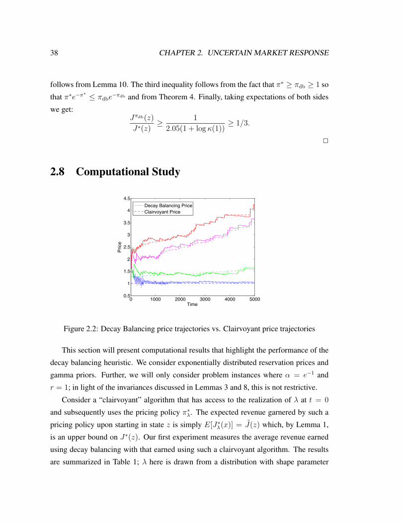
38 CHAPTER 2. UNCERTAIN MARKET RESPONSE
follows from Lemma 10. The third inequality follows from the fact that π∗ ≥ πdb ≥ 1 so
that π∗e−π∗ ≤ πdbe−πdb and from Theorem 4. Finally, taking expectations of both sides
we get:Jπdb(z)
J∗(z)≥ 1
2.05(1 + log κ(1))≥ 1/3.
2
2.8 Computational Study
0 1000 2000 3000 4000 50000.5
1
1.5
2
2.5
3
3.5
4
4.5
Time
Price
Decay Balancing PriceClairvoyant Price
Figure 2.2: Decay Balancing price trajectories vs. Clairvoyant price trajectories
This section will present computational results that highlight the performance of the
decay balancing heuristic. We consider exponentially distributed reservation prices and
gamma priors. Further, we will only consider problem instances where α = e−1 and
r = 1; in light of the invariances discussed in Lemmas 3 and 8, this is not restrictive.
Consider a “clairvoyant” algorithm that has access to the realization of λ at t = 0
and subsequently uses the pricing policy π∗λ. The expected revenue garnered by such a
pricing policy upon starting in state z is simply E[J∗λ(x)] = J(z) which, by Lemma 1,
is an upper bound on J∗(z). Our first experiment measures the average revenue earned
using decay balancing with that earned using such a clairvoyant algorithm. The results
are summarized in Table 1; λ here is drawn from a distribution with shape parameter

2.8. COMPUTATIONAL STUDY 39
1 2 3 4 5 6 7 8 9 100 %
10%
20%
30%
40%Performance Gain over Certainty Equivalent Heuristic
Initial Inventory Level
% G
ain
1 2 3 4 5 6 7 8 9 100%
100%
200%
300%Performance Gain over Greedy Pricing
Initial Inventory Level
% G
ain
Figure 2.3: Performance gain over the Certainty Equivalent and Greedy Pricing heuristicsat various inventory levels
a = 0.04 and scale parameter b = 0.001 which corresponds to a mean of 40 and a
coefficient of variation of 5. These parameter values are representative of a high level of
uncertainty in λ. As is seen in Table 1, the performance of the decay balancing heuristic
is surprisingly close to that of the clairvoyant algorithm.
We next record price trajectories realized using decay balancing for several widely
different realizations of λ. We compare these trajectories with the prices set by a clair-
voyant algorithm. In particular, for a given state trajectory realized under the use of the
decay balancing heuristic, zt, we plot πdb(zt) along side π∗λ(zt). The decay balancing
heuristic begins with a prior with mean 50 and coefficient of variation 4.47. Figure 2.2
plots decay balancing price trajectories for λ = 10, 50, 200, and 400 along side the
optimal clairvoyant price for each trajectory. From lowest to highest, the curves corre-
spond respectively to λ = 10, 50, 200, and 400. First, it is satisfying to note that the
decay balancing price tracks the clairvoyant price closely. Second, we note that each of
the price trajectories have relatively stable trends which is desirable from an operational
perspective. In contrast, price trajectories realized by a non-parametric pricing algorithm

40 CHAPTER 2. UNCERTAIN MARKET RESPONSE
Table 2.3: Performance vs. a Clairvoyant algorithm
Inventory Level x0 = 1 x0 = 2 x0 = 5 x0 = 10 x0 = 20 x0 = 40
Performance Gain −13% −10% −6% −3.7% −2% −0.5%i.e. (Jπdb − J)/J
such as Besbes and Zeevi (2006) will vary substantially over periods corresponding to
price-experimentation since such an algorithm needs to experiment with essentially ev-
ery possible price. Finally, these trajectories are also an indicator of robustness to our
choice of prior; πdb when λ = 400 (the topmost solid curve) tracks π∗400 (the topmost
dashed curve) in spite of starting with a prior mean that is smaller than the actual arrival
rate by an order of magnitude!
We finally turn to comparing the performance of decay balancing against that of
the certainty equivalent and greedy policies. We first compare gain in performance
over the certainty equivalent heuristic and the greedy policy for inventory levels be-
tween 1 and 10. We set a = 0.05 and b = 0.001 for all heuristics, corresponding to
a mean of 50 and a coefficient of variation of 4.47. Now E[λ]/α can be interpreted as
the expected number of potential customers encountered over the sales season. Con-
sequently, E[λ]/α divided by the inventory level may be viewed as the “load factor”
here. Figure 2.3 indicates that we offer a substantial gain in performance over the cer-
tainty equivalent and greedy pricing heuristics at higher load factors (approximately 2
for these experiments) which is representative of a regime wherein judiciously managing
inventory levels is crucial. The greedy policy performs particularly poorly. In addi-
tion, as discussed earlier, that policy exhibits qualitative behavior that is clearly subopti-
mal: for a problem with mean reservation price 1 and discount factor e−1, we compute
πgp(1, 0.1, 0.1)(= 1.26) < πgp(4, 0.1, 0.1)(= 1.61) > πgp(10, 0.1, 0.1)(= 1.25) so that,
all other factors remaining the same, prices may increase or decrease with an increase in
inventory level. Our gain in performance falls at lower load factors. This is not surpris-
ing; intuitively, the control problem at hand is simpler at low load factors since we are
essentially allowed to sacrifice a few units of inventory early on so as to learn quickly

2.9. DISCUSSION AND CONCLUSIONS 41
without incurring much of a penalty. We next present a lower bound on highest poten-
tial performance gain for various coefficients of variation of the initial prior on λ. See
Figure 2.4 wherein the data point for each coefficient of variation c, corresponds to an
experiment with a = 1/c2, b = 0.001 (which corresponds to a mean of 1000/c2), and
an inventory level of 1 and 2 for the certainty equivalent and greedy pricing heuristics
respectively. These experiments indicate that the potential gain from using decay bal-
ancing increases with increasing uncertainty in λ, and that in fact the gain over certainty
equivalence can be as much as a factor of 1.3, and that over the greedy policy can be as
much as a factor of 3.
To summarize our computational experience, the performance of decay balancing is
surprisingly competitive with that of a clairvoyant algorithm even at high levels of un-
certainty, so that we suspect decay balancing is near optimal. In comparison with other
available heuristics (namely certainty equivalent and greedy) decay balancing offers sub-
stantial performance gains especially at high load factors. Finally, the performance gains
offered by decay balancing over these competing heuristics increase with increasing un-
certainty in customer arrival rate.
2.9 Discussion and Conclusions
The dynamic pricing model proposed by Gallego and van Ryzin (1994) is central to a
large body of the revenue management literature. This chapter considered an important
extension to that model. In particular, we considered incorporating uncertainty in the
customer arrival rate or “market response” which is without doubt important in many
industries that practice revenue management, but whose effects are nonetheless ignored
in “estimate, then optimize” style pricing schemes.
We proposed and analyzed a simple new heuristic for this problem: decay balancing.
Decay balancing is computationally efficient and leverages the solution to problems with
no uncertainty in market response. Our computational experiments (which focused on
gamma priors and exponentially distributed reservation prices) suggest that decay balanc-
ing achieves near-optimal performance even on problems with high levels of uncertainty
in market response. Pricing policies generated by decay balancing have the appealing

42 CHAPTER 2. UNCERTAIN MARKET RESPONSE
structural property that, all other factors remaining the same, the price in the presence of
uncertainty in market response is higher than the corresponding price with no uncertainty
. This is reasonable from an operational perspective and is in fact a property possessed
by the optimal policy. Uncertainty in market response could qualitatively induce two
potential price movements: whereas on the one hand, the revenue manager may wish to
price lower than the no-uncertainty price in an effort to eliminate uncertainty as quickly
as possible, he may on the other hand want to hedge against the possibility that market
response is in fact stronger than expected by pricing higher than the no-unceratinty price
and protecting inventory for this eventuality. It is interesting to note that this second
hedging effect dominates irrespective of the level of uncertainty. Finally, our analysis
demonstrated a uniform performance guarantee for decay balancing when reservation
prices are exponentially distributed, which is an indicator of robustness.
Two heuristics proposed for problems of this nature prior to our work were the cer-
tainty equivalent heuristic (by Aviv and Pazgal (2005)) and the greedy pricing heuristic
(by Araman and Caldentey (2005)). Our computational results suggest that decay bal-
ancing offers significant performance advantages over these heuristics. These advantages
are especially clear at high levels of uncertainty in market response which is arguably the
regime of greatest interest. Decay balancing relies only on a good approximation to the
value of an optimal policy at a given state. This is in contrast with greedy pricing that
requires not only a good approximation to value but further to derivatives of value with
respect to the scale parameter. At the same time, uncertainty in arrival rate and changes
in inventory levels bear the appropriate directional impact on decay balancing prices:
uncertainty in the arrival rate calls for higher prices than in corresponding situations with
no uncertainty, while a decrease in inventory calls for an increase in prices. In contrast,
uncertainty in the arrival rate has no impact on certainty equivalent prices while greedy
prices can increase or decrease with decreasing inventory.
Our computational study and performance analysis were focused on exponentially
distributed reservation prices and gamma priors, but we expect favorable performance
for other distributions as well. In particular, the analysis of Theorem 3 can be extended
to mixtures of Gamma priors yielding encouraging estimates on the quality of approxi-
mation provided by J . Since the decay balancing price at state z is likely to be a good

2.9. DISCUSSION AND CONCLUSIONS 43
approximation to the optimal price at z if J(z) is a good approximation to J∗(z), this
suggests that decay balancing is likely to do a good job of approximating the optimal
price for general reservation price distributions and priors on arrival rate, which in turn
should lead to superior performance.
There is ample room for further work in the general area of pricing with uncertainty
in market response and other factors that impact demand. One direction is considering
more complex models. The next chapter makes a foray in this direction. In particu-
lar, that chapter will consider two interesting models closely related to the model we
focused on here, that allows for the modeling of joint learning from sales at multiple
locations and product “versioning” respectively. There are other models one might hope
to consider. For example, the multi product model proposed by Gallego and van Ryzin
(1997). Another potential direction is exploring new approximations to the value func-
tion beyond the approximation considered here and applying such approximations with
either the greedy pricing or decay balancing heuristics. Finally, it would be interesting to
extend the approaches in this chapter to problems with uncertainty in other factors that
impact demand such as price elasticity.

44 CHAPTER 2. UNCERTAIN MARKET RESPONSE
0 1 2 3 4 5 6−5%
0%
5%
10%
15%
20%
25%
30%
35%
40%
45%
Coefficient of Variation of Initial Prior
% G
ain
Maximal Performance Gain over Certainty Equivalent heuristic
Estimated gain98% confidence upper bound98% confidence lower bound
0 1 2 3 4 5 60%
50%
100%
150%
200%
250%
300%
350%
Coefficient of Variation of Initial Prior
% G
ain
Maximal Performance Gain over Greedy Pricing heuristic
Estimated gain98% confidence upper bound98% confidence lower bound
Figure 2.4: Maximal performance gain over the Certainty Equivalent Heuristic (left) andGreedy Heuristic (right) for various coefficients of variation

Chapter 3
Decay Balancing Extensions
The previous chapter developed a “decay balancing” heuristic in the context of a simple
one product dynamic pricing problem. This chapter explores generalizing that heuris-
tic to two closely related problems of dynamic pricing with demand uncertainty. In
particular, we consider a problem of dynamic pricing across multiple stores with un-
interchangeable inventories, where stores attempt to learn from each others’ purchase
data. We also consider a problem of dynamic pricing with product “versioning”: a single
product may be sold in multiple versions. Customers arrive at an uncertain rate and must
choose from among these versions according to a pre-specified demand model. The rev-
enue manager would like to set prices for all of the product versions over time so as to
maximize expected discounted revenues.
3.1 Multiple Stores and Consumer Segments
We consider in this section a model with multiple stores and consumer segments. We do
not attempt to extend our performance analysis to this more general model but instead
present numerical experiments, the goal being to show that decay balancing demonstrates
the same qualitative behavior as in the one store, one customer segment case we have
studied to this point.
More formally, we consider a model with N stores and M consumer segments. Each
store is endowed with an initial inventory x0,i for i ∈ {1, . . . , N}. Customers from class
45

46 CHAPTER 3. DECAY BALANCING EXTENSIONS
j, for j ∈ {1, . . . ,M} arrive according to a Poisson process of rate λj where λj is a
Gamma distributed random variable with shape parameter a0,j and scale parameter b0,j .
An arriving segment j customer considers visiting a single store and will consider store
i with probability αij . Consequently, each store i sees a Poisson stream of customers
having rate∑
j αijλj . We assume without loss of generality that∑
i αij = 1. We as-
sume that customers in each segment have exponential reservation price distributions
with mean r and moreover that upon a purchase the store has a mechanism in place to
identify what segment the purchasing customer belongs to.
Let pt ∈ RN , t ∈ [0,∞) represent the process of prices charged at the stores over
time. Let njt,i represent the total number of type j customers served at store i up to time
t and let njt =
∑i n
jt,i. The parameter vectors a and b are then updated according to:
at,j = a0,j + nt,j and bt,j = b0,j +
∫ t
τ=0
∑i
e−pτ,i/rdτ
Our state at time t is now zt = (xt, at, bt). As before, we will consider prices gener-
ated by policies π that are measurable, non-negative vector-valued functions of state, so
that pt = π(zt) ≥ 0. Letting Π denote the set of all such policies, our objective will be
to identify a policy π∗ ∈ Π that maximizes
Jπ(z) = Ez,π
[∑i
∫ τ i
0
ρt,ie−pt,i/rdt
]
where τ i = inf{t :∑
j njt,i = x0,i} and ρi =
∑j αi,j(aj/bj). We define the operator
(HπJ)(z) =∑i
[ρie
−π(z)i/r
(π(z)i +
∑j
αi,j(aj/bj)
ρi
J(x− ei, a+ ej, b)− J(z)
)
+∑
j
e−π(z)i/r d
dbjJ(z)
]− αJ(z).
where ek is the vector that is 1 in the kth coordinate and 0 in other coordinates. One may

3.1. MULTIPLE STORES AND CONSUMER SEGMENTS 47
show that J∗ = Jπ∗ is the unique solution to
supπ∈Π
(HπJ)(z) = 0 ∀z
satisfying J∗(0, a, b) = 0, and that the corresponding optimal policy for xi > 0 is given
by
(π∗(z))i =
r + J∗(z)−∑
j
αi,j(aj/bj)
ρi
J∗(x− ei, a+ ej, b)−1
ρi
∑j
d
dbjJ∗(z).
(3.1)
Now, assuming that the λj’s are known perfectly a-priori, it is easy to see that the
control problem decomposes across stores. In particular, the optimal strategy simply
involves store i using as it’s pricing policy
pt,i = π∗ρi(xt,i)
where ρi =∑
j αi,jλj . Consequently, a certainty equivalent policy would use the pricing
policy
(πCE(z))i = π∗ρi(xi)
We can also consider as an approximation to J∗, the following upper bound (which is in
the spirit of the upper bound we derived in Section 3):
J(z) = E
[∑i
J∗ρi(xi)
].
The analogous greedy pricing policy πgp is then given by (3.1) upon substituting J(·) for
J∗(·) in that expression.
Motivated by the decay balancing policy derived for the single store case we consider
using the following pricing policy at each store:
(πdb(z))i = r log
(rρi
αE[J∗ρi(xi)]
).

48 CHAPTER 3. DECAY BALANCING EXTENSIONS
1 22
4488
1122
4488
−12%
−10%
−8%
−6%
−4%
−2%
Store 1 Inventory
Performance Gain over Clairvoyant Algorithm
Store 2 Inventory
% G
ain
Figure 3.1: Performance relative to a clairvoyant algorithm
Such a heuristic involves joint learning across stores and continues to account for the
level of uncertainty in the pricing process. Further, the structural properties discussed in
the single store case are retained. The joint learning under this heuristic does not however
account for inventory levels across stores.
We now present computational results for the three heuristics. Our experiments will
use the following model parameters. We take N = 2,M = 2 and assume αi,j = 1/2
for all i, j, and further that we begin with prior parameters a1 = a2 = 0.04, and
b1 = b2 = 0.001 (which corresponds to a mean of 40 and a coefficient of variation
of 5). As usual, α = e−1, r = 1. Our first set of results (Figure 3.1) compares the de-
cay balancing heuristic’s performance against that of a clairvoyant algorithm which as
in Section 2.8 has perfect a-priori knowledge of λ. As in the N = 1,M = 1 case, our
performance is quite close to that of the clairvoyant algorithm. Figure 3.2 compares de-
cay balancing performance to the certainty equivalent heuristic and the greedy heuristic.
Figure 3.2 is indicative of performance that is qualitatively similar to that observed for
the N = 1,M = 1 case; there is a significant gain over certainty equivalence at lower
inventory levels, but this gain shrinks as inventory level increases. The performance of
the greedy heuristic is particularly dismal, one explanation for which is that∑
jd
dbjJ(z)
is a potentially poor approximation to∑
jd
dbjJ∗(z).
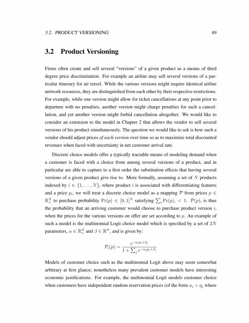
3.2. PRODUCT VERSIONING 49
3.2 Product Versioning
Firms often create and sell several “versions” of a given product as a means of third
degree price discrimination. For example an airline may sell several versions of a par-
ticular itinerary for air travel. While the various versions might require identical airline
network resources, they are distinguished from each other by their respective restrictions.
For example, while one version might allow for ticket cancellations at any point prior to
departure with no penalties, another version might charge penalties for such a cancel-
lation, and yet another version might forbid cancellation altogether. We would like to
consider an extension to the model in Chapter 2 that allows the vendor to sell several
versions of his product simultaneously. The question we would like to ask is how such a
vendor should adjust prices of each version over time so as to maximize total discounted
revenues when faced with uncertainty in net customer arrival rate.
Discrete choice models offer a typically tractable means of modeling demand when
a customer is faced with a choice from among several versions of a product, and in
particular are able to capture to a first order the substitution effects that having several
versions of a given product give rise to. More formally, assuming a set of N products
indexed by i ∈ {1, . . . , N}, where product i is associated with differentiating features
and a price pi, we will treat a discrete choice model as a mapping P from prices p ∈RN
+ to purchase probability Pr(p) ∈ [0, 1]N satisfying∑
i Pr(p)i < 1. P(p)i is thus
the probability that an arriving customer would choose to purchase product version i,
when the prices for the various versions on offer are set according to p. An example of
such a model is the multinomial Logit choice model which is specified by a set of 2N
parameters, α ∈ RN+ and β ∈ RN , and is given by:
Pi(p) =e−αipi+βj
1 +∑
j e−αjpj+βj
Models of customer choice such as the multinomial Logit above may seem somewhat
arbitrary at first glance; nonetheless many prevalent customer models have interesting
economic justifications. For example, the multinomial Logit models customer choice
when customers have independent random reservation prices (of the form uj + ηj where

50 CHAPTER 3. DECAY BALANCING EXTENSIONS
ηj is a certain extreme valued random variable) for the various product versions, and
make choices that maximize their surplus. Ben-Akiva and Lerman (1985) provides an
interesting discussion of various choice models that may be used in modeling situations
such as the product versioning example under consideration.
3.2.1 Problem Formulation
We consider the following extension to the model with uncertain arrival rates of Chapter
2. The vendor is endowed with a finite initial inventory x0 ∈ Z+ of a product and
chooses to sell N versions of the product. Customers arrive at a rate λ where λ is a
Gamma distributed random variable with parameters a and b. Upon arrival the customer
faces a choice among the N product versions priced according to p ∈ RN+ . The customer
chooses at most one product version for purchase; version i is chosen with probability
P(p)i, and we denote by I(p) the random index of the chosen version. The vendor sets
a vector of prices pt ∈ RN+ over time t ∈ [0,∞). Letting nt denote the total number of
sales up to time t, the vendor updates the parameters of his prior on arrival rate according
to
at = a0 + nt and bt = b0 +
∫ t
0
θτdτ
where θτ =∑
iP(pτ )i.
From a control standpoint, our state is now zt = (xt, at, bt), and as in Chapter 2 we
will consider prices generated by policies π that are measurable, non-negative, vector
valued functions of state, so that pt = π(zt) ≥ 0. Letting Π denote the set of all such
policies, our objective will be to identify a policy π∗ ∈ Π that maximizes
Jπ(z) = Ez,π
[∫ τ0
0
pt,I(pt)dnt
]= Ez,π
[∫ τ0
0
∑i
P(pt)ipt,iλdt
]
where we use the fact that the sales process for product version i is Poisson of instanta-
neous rate λP(pt)i.

3.2. PRODUCT VERSIONING 51
3.2.2 Optimal pricing
For each policy π ∈ Π, we define an operator
(HπJ)(z) =∑
i
µ(z)P(π(z))i
(π(z)i + J(z′)− J(z) +
1
µ(z)
d
dbJ(z)
)− αJ(z)
where z′ = (x− 1, a+ 1, b). Assuming that there exists a solution J∗ ∈ J to
supπ∈Π
(HπJ)(z) = 0 ∀z
it is straight forward to show that this solution is unique and that J∗ = Jπ∗ . Further, the
optimal policy requires
π∗(z) ∈ argmaxπ(z)
∑i
µ(z)P(π(z))i
(π(z)i + J(z′)− J(z) +
1
µ(z)
d
dbJ(z)
)
We note that in the absence of uncertainty in λ, the corresponding HJB equation is in
fact reduced to a simple recursion via which computing J∗λ is a computationally tractable
task.
While the preceding formulation is natural, it has the disadvantage of requiring the
solution to a control problem with anN -dimensional action space. An alternative, equiv-
alent view of the optimal control problem at hand with a one-dimensional action space is
the following: At each point in time, the vendor picks θt ∈ [0, β], the fraction of arriving
customers that will make a purchase of some version. Here β = maxp∈RN+
∑iP(p)i, the
maximal arrival rate that the seller can induce. One may then assume without loss that he
should set prices pt = p∗(θt) ∈ argmaxp:P
i P(p)i=θt
∑iP(p)ipi. We may consequently
view a policy π as a measurable mapping from state to the interval [0, β] and we denote
by Π the set of all such policies.
Define the expected revenue from a sale upon taking action θ asR(θ) =∑
ip∗(θ)iP(p∗(θ))iP
i P(p∗(θ))i.
We make the following assumptions on the functions R(·) and ·R(·):
Assumption 3. R(·) is a bounded, differentiable function and ·R(·) is a strictly concave

52 CHAPTER 3. DECAY BALANCING EXTENSIONS
function on the interval [0, β].
We next define for each policy π, the operator:
(H πJ)(z) = µ(z)π(z)
(R(π(z)) + J(z′)− J(z) +
1
µ(z)
d
dbJ(z)
)− αJ(z).
Now, assuming that there exists a solution J∗ ∈ J to
supπ∈Π
(H πJ)(z) = 0 ∀z
it is straight forward to show that this solution is unique and that J∗ = Jπ∗ .
3.2.3 Decay Balancing
A solution J∗ to the HJB equation (for our second formulation) must satisfy:
supθ∈[0,β]
µ(z)θ
(R(θ) + J∗(z′)− J∗(z) +
1
µ(z)
d
dbJ∗(z)
)= αJ∗(z) (3.2)
Now, if θ∗ attains the maximum in the equation above, and assuming that this maximum
is always attained in (0, β), the first order optimality conditions are by Assumption 3
necessary and sufficient, and imply that
−(θ∗)2R′(θ∗) =αJ∗(z)
µ(z)
This is a decay balance equation for the dynamic pricing problem with product ver-
sioning. Now by Assumption 3, the optimal control problem at hand has a unique opti-
mizing policy in Π (that is, the maximizing set for the left hand side of (3.2) is a single-
ton), so that the decay balance equation at state z has a unique solution θ(z) on (0, β)
with θ(z) = θ∗(z). p∗(θ(z)) is then the optimal price vector in state z.
Of course, since we do not know J∗ we could consider using the same approximation
to J∗ as in the previous section, J(z) = E[J∗λ(z)]. The decay balance heuristic price in

3.3. DISCUSSION 53
state z is then p∗(θdb(z)) where θdb(z) solves
−(θdb(z))2R′(θdb(z)) =
αJ(z)
µ(z)
If J(z) is a good approximation to J∗(z), p∗(θdb(z)) is likely to be a good approximation
to p∗(θ∗(z)) and one would expect similar levels of performance as in the one product
case studied in Chapter 2.
3.3 Discussion
Decay balancing type heuristics should typically be useful in deriving pricing policies
for problems with uncertainty in a single parameter and a one dimensional control. This
chapter attempted to generalize the heuristic to other situations. The product versioning
problem nominally requires an N -dimensional control, but our development took ad-
vantage of the fact that the optimal control problem may be reduced to one with a one
dimensional control. For the problem with multiple stores and consumer segments, our
use of the decay balancing heuristic was ad-hoc and motivated by the single store solu-
tion of Chapter 2, but nonetheless yielded promising computational results. There are
several other formulations for which we believe decay balancing might well yield useful
pricing heuristics including problems with uncertainty in demand elasticity (as opposed
to market response), or the finite time horizon version of the problem in Chapter 2.
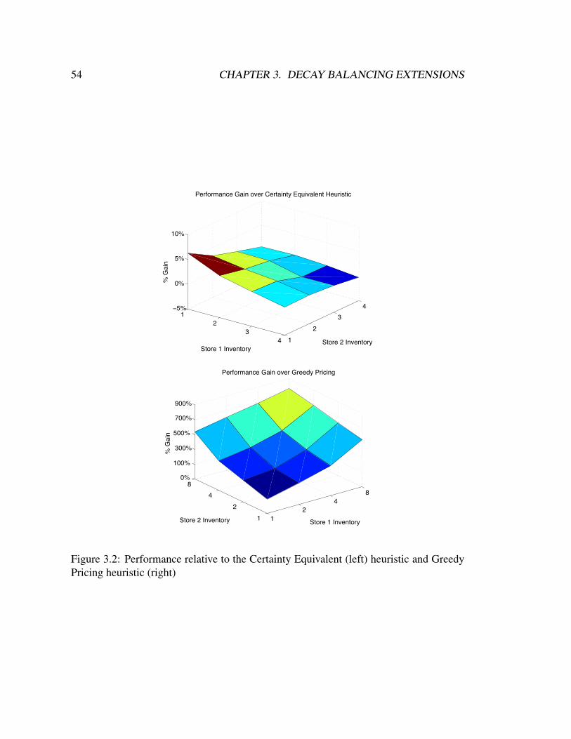
54 CHAPTER 3. DECAY BALANCING EXTENSIONS
12
34 1
23
4−5%
0%
5%
10%
Store 2 Inventory
Performance Gain over Certainty Equivalent Heuristic
Store 1 Inventory
% G
ain
1 2
48
1 2
4 8
0%
100%
300%
500%
700%
900%
Store 1 Inventory
Performance Gain over Greedy Pricing
Store 2 Inventory
% G
ain
Figure 3.2: Performance relative to the Certainty Equivalent (left) heuristic and GreedyPricing heuristic (right)

Chapter 4
Network-RM with Forecast Models
This chapter focuses on a problem of airline Network-RM. In contrast to the dynamic
pricing problems studied in Chapters 2 and 3, demand in the airline industry is far more
predictable and fairly well modeled. Most airlines have access to complex forecast mod-
els estimated on the basis of large quantities of relevant historical data. The “Estimate,
Then Optimize” heuristic in this context entails the use of optimization algorithms that in
the interest of tractability make simplifying assumptions of demand. In doing so, the rev-
enue manager is typically unable to harness all the predictive capabilities of the forecast
models available to him.
We develop in this chapter an approximation algorithm for a dynamic capacity allo-
cation problem with Markov modulated customer arrival rates (the typical simplifying
assumption made in solving such optimization problems is that demand is determinis-
tic and equal to expected forecasted demand). For each time period and each state of
the modulating process, the algorithm approximates the dynamic programming value
function using a concave function that is separable across resource inventory levels. We
establish via computational experiments that our algorithm increases expected revenue,
in some cases by close to 8%, relative to a deterministic linear program that is widely
used for bid-price control.
55

56 CHAPTER 4. NETWORK-RM WITH FORECAST MODELS
4.1 Introduction
Network revenue management refers to the activity of a vendor who is endowed with
limited quantities of multiple resources and sells products, each composed of a bundle of
resources, controlling their availability and/or prices over time with an aim to maximize
revenue. The airline industry is perhaps the most notable source for such problems. An
airline typically operates flights on each leg of a network of cities and offers for sale
“fare products” composed of seats on one or more of these legs. Each fare product is
associated, among other things, with some fixed price which the airline receives upon its
sale. Since demand for fare products is stochastic and capacity on each leg limited, the
airline’s problem becomes one of deciding which of its fare products to offer for sale at
each point in time over a finite sales period so as to maximize expected revenues. This
chapter presents a new algorithm for this widely studied problem.
For most models of interest, the dynamic capacity allocation problem we have de-
scribed can be cast as a dynamic program, albeit one with a computationally intractable
state-space even for networks of moderate size. As such, revenue management tech-
niques have typically resorted to heuristic control strategies. Early heuristics for the
problem were based primarily on the solutions to a set of single resource problems solved
for each leg. Today’s state of the art techniques involve “bid-price” control. A generic
bid-price control scheme might work as follows: At each point in time the scheme gen-
erates a bid-price for a seat or unit of capacity on each leg of the network. A request for a
particular fare product at that point in time is then accepted if and only if the revenue gar-
nered from the sale is no smaller than the sum of the bid prices of the resources or seats
that constitute that fare product. There is a vast array of available algorithms that may be
used in the generation of bid-prices. There are two important dimensions along which
such an algorithm must be evaluated. One, of course, is revenues generated from the
strategy. Since bid-prices must be generated in real time, a second important dimension
is the efficiency of the procedure used to generate them. A simple approach to this prob-
lem which has found wide-spread acceptance involves the solution of a single linear pro-
gram referred to as the deterministic LP (DLP). This approach and associated bid-price
techniques have found widespread use in modern revenue management systems and are

4.1. INTRODUCTION 57
believed to have generated incremental revenues on the order of 1-2% greater than previ-
ously used “fare-class” level heuristics (see P.P.Belobaba and Lee (2000), P.P.Belobaba
(2001)).
The algorithm we present applies to models with Markov-modulated customer ar-
rival rates. This represents a substantial generalization of the deterministic arrival rate
arrival process models generally considered in the literature and accommodates a broad
class of demand forecasting models. We demonstrate via a sequence of computational
examples that our algorithm consistently produces higher revenues than a strategy using
bid-prices computed via re-solution of the DLP at each time step. While the performance
gain relative to the DLP is modest (∼ 1%) for a model with time homogeneous arrivals,
this gain increases significantly when arrival rates vary stochastically. Even for a simple
arrival process in which the modulating process has three states, we report relative per-
formance gains of up to about 8% over a DLP approach suitably modified to account for
the stochasticity in arrival rates.
Our algorithm is based on a linear programming approach to approximate dynamic
programming (de Farias and Van Roy (2003), de Farias and Van Roy (2004)). A lin-
ear program is solved to produce for each modulating process state and each time an
approximation to the optimal value function that is separable across resource inventory
levels. A heuristic is then given by the greedy policy with respect to this approximate
value function. This policy can be interpreted in terms of bid-price control for which bid
prices are generated at each point in time via a table look-up, which takes far less time
than solving the DLP.
The ALP has as many constraints as the size of the state space and practical solution
requires a constraint sampling procedure. We exploit the structural properties afforded
by our specific approximation architecture to derive a significantly simpler alternative
(the rALP) for which the number of constraints grows linearly with maximal capacity
on each network leg. The rALP generates a feasible solution to the ALP. We show that
this solution is optimal for affine approximations. While we aren’t able to prove that
this solution is optimal for concave approximations, the rALP generates optimal ALP
solutions in all of our computational experiments with that architecture as well. The
rALP thus significantly enhances the scalability of our approach.

58 CHAPTER 4. NETWORK-RM WITH FORECAST MODELS
The literature on both general dynamic capacity allocation heuristics, as well as bid-
price controls is vast and predominantly computational; Talluri and van Ryzin (2004)
provides an excellent review. Closest to this work is the paper by Adelman (2005), which
also proposes an approximate DP approach to computing bid prices via an affine approx-
imation to the value function. The rALP we propose allows an exponential reduction in
the number of constraints for the ALP with affine approximation. However, in spite of
affine approximation being a computationally attractive approximation architecture, our
computational experiments suggest that affine approximations are not competitive with
an approach that uses bid-prices computed via re-solution of the DLP at each time step.
Our approach might be viewed as a means of generating bid-prices. There have been
a number of algorithms and heuristics proposed for this purpose. One class of schemes
is based on mathematical programming formulations of essentially static versions of the
problem that make the simplifying assumption that demand is deterministic and equal to
its mean. The DLP approach is representative of this class and apparently the method of
choice in practical applications (Talluri and van Ryzin (2004)). We compare the perfor-
mance of our approach to such a scheme. Highly realistic simulations in P.P.Belobaba
(2001) suggest that this class of approaches generates incremental revenues of approxi-
mately 1-2% over earlier leg-based RM techniques. There are alternatives to the use of
bid price controls, the most prominent among them being “virtual nesting” schemes such
as the displacement adjusted (DAVN) scheme (see Talluri and van Ryzin (2004)). We do
not consider our performance relative to such schemes; a subjective view (E. A. Boyd
(2005)) is that these schemes are consistently outperformed by bid-price based schemes
in practice.
An important thrust of our work is the incorporation of Markov-modulated customer
arrival processes. There is an emerging literature on optimization techniques for models
that incorporate demand processes where arrival rates are correlated in time. A recent
example is the paper by de Miguel and Mishra (2006), that evaluates various multi-stage
stochastic programming techniques for a linear (with additive noise) model of demand
evolution. These approaches rely on building “scenario-trees” based on simulations of
demand trajectories. While they can be applied to Markov-modulated arrival processes,

4.2. MODEL 59
scenario trees and their associated computational requirements typically grow exponen-
tially in the horizon.
The remainder of this chapter is organized as follows: In section 2, we formally
specify a model for the dynamic capacity allocation problem. In section 3 we review
the benchmark DLP heuristic. Section 4 presents an ADP approach to the dynamic
capacity allocation problem and specifies our approximation architecture. That section
also discusses some simple structural properties possessed by our approximation to the
value function. Section 5 presents a series of computational examples comparing the
performance of our algorithm with the DLP approach as also an approach based on an
affine approximation to the value function. Section 6 studies a simple scalable alternative
to the ALP, the rALP, and discusses computational experience with that program. Section
7 concludes.
4.2 Model
We consider an airline operating L flight legs. The airline may offer up to F fare products
for sale at each point in time. Each fare product f is associated with a price pf and
requires seats on one or more legs. A matrix A ∈ ZL×F+ encodes the capacity on each
leg consumed by each fare product: Al,f = k if and only if fare product f requires k
seats on leg l. For concreteness we will restrict attention to the situation wherein a given
fare product can consume at most 1 seat on any given leg although our discussion and
algorithms carry over without any change to the more general case. Initial capacity on
each leg is given by a vector x0 ∈ ZL+. Time is discrete. We assume an N period horizon
with at most one customer arrival in a single period. A customer for fare product f arrives
in the nth period with probability λf (mn). Heremn ∈M (a finite set) and represents the
current demand “mode”. mn evolves according to a discrete time Markov process onMwith transition kernel Pn. We note that the discrete time arrival process model we have
described may be viewed as a uniformization of an appropriately defined continuous time
arrival process. At the start of the nth period the airline must decide which subset of fare
products from the set {f : Af � xn} it will offer for sale; an arriving customer for fare
product f is assigned that fare product should it be available, the airline receives pf , and

60 CHAPTER 4. NETWORK-RM WITH FORECAST MODELS
xn+1 = xn − Af .
We define the state-space S = {x : x ∈ ZL+, x � x0} × {0, 1, 2, . . . , N} × M.
Encoding the fare products offered for sale at time n by a vector in {0, 1}F ≡ A, a
control policy is a mapping π : S → A satisfying Aπ(s) ≤ x(s) for all s ∈ S. Let
Π represent the set of all such policies. Let R(s, a) be a random variable representing
revenue generated by the airline in state s ∈ S when fare products a ∈ A are offered for
sale, and define for s ∈ S ,
Jπ(s) = Eπ
N−1∑n′=n(s)
R(sn′ , π(sn′))∣∣sn(s) = s
.We let J∗(s) = maxπ∈Π J
π(s), denote the expected revenue under the optimal policy π∗
upon starting in state s.
J∗ and π∗ can, in principle, be computed via Dynamic Programming. In particular,
define the dynamic programming operator T for s ∈ {s′ : n(s′) < N − 1} according to
(TJ)(s) =∑
f :Af≤x(s)
λf (m(s)) max[pf + E
[J(S ′f)], E [J (S ′)]
]+(1−
∑f :Af≤x(s)
λf (m(s)))E [J(S ′)] .
(4.1)
where S ′f = (x(s) − Af , n(s) + 1,mn(s)+1) and S ′ = (x(s), n(s) + 1,mn(s)+1).
For s ∈ {s′ : n(s′) = N − 1} we define (TJ)(s) =∑
f :Af≤x(s) λf (m(s))pf . We
define (TJ)(s) = 0 for all s ∈ {s′ : n(s′) = N}. J∗ may then be identified as the
unique solution to the fixed point equation TJ = J . π∗ is then the policy that achieves
the maximum in (4.1); in particular, π∗(s)f = 0 iff pf + E[J(S ′f )
]< E [J (S ′)] and
n(s) < N − 1.
We will focus on three special cases of the above model, with N assumed even for
notational convenience:
• (M1) Time homogeneous arrivals: Here we have |M| = 1. That is the arrival
rate of customers for the various fare products is constant over time and the arrival

4.3. BENCHMARK HEURISTIC: THE DETERMINISTIC LP (DLP) 61
process is un-correlated in time.
• (M2) Multiple demand modes, deterministic transition time: Here we consider
a model with M = {med,hi,lo}. We have mn = med for n ≤ N/2. With
probability p, mn = lo for all n > N/2 and with probability 1 − p and mn = hi
for all n > N/2. This is representative of a situation where there is likely to be a
change in arrival rates at some known point during the sales season. The revenue
manager has a probabilistic model of what the new arrival rates are likely to be.
• (M3) Multiple demand modes, random transition time: Here we consider a model
with M = {med, hi,lo}, with the transition kernel Pt defined according to
Pn(mn+1 = y|mn = x) =
1− q qp q(1− p)
0 1 0
0 0 1
xy
.
where q, p ∈ (0, 1). This arrival model is similar to the second with the exception
that instead of a change in demand modes occurring at precisely n = N/2, there
is now uncertainty in when this transition will occur. In particular, the transition
time is now a geometric random variable with expectation 1/q.
The above models were chosen since they are simple and yet serve to illustrate the rela-
tive merits of our approach for Markov-modulated demand processes.
4.3 Benchmark Heuristic: The Deterministic LP (DLP)
The Dynamic Programming problem we have formulated is computationally intractable
and so one must resort to various sub-optimal control strategies. We review the DLP-
heuristic for generating bid prices. This heuristic makes the simplifying assumption that
demand is deterministic and equal to its expectation. In doing so, the resulting control
problem reduces to the solution of a simple LP (the DLP) and the optimal control policy
is static. In particular, if demand for fare product f over aN−n period sales season,Dn,f ,
were deterministic and equal to expected demand, E[Dn,f |mn], the maximal revenue that

62 CHAPTER 4. NETWORK-RM WITH FORECAST MODELS
one may generate with an initial capacity x(s) is given by the optimal solution to the
DLP:
DLP (s) : max p′z
s. t. Az ≤ x(s)
0 ≤ z ≤ E[Dn(s)|mn(s) = m(s)]
Denote by r∗(s) a vector of optimal shadow prices corresponding to the constraint
Az ≤ x(s) in DLP (s). The bid price control policy based on the DLP solution is then
given by:
πDLP(s)f =
{1 if A′
fr∗(s) ≤ pf and Af ≤ x(s)
0 otherwise
The above description of the DLP heuristic assumes that the shadow prices r∗ are
recomputed at each time step. While this many not always be the case, a general com-
putational observation according to Talluri and van Ryzin (2004) is that frequent re-
computation of r∗ improves performance. This is consistent with our computational
experience.
In the case of model M2, one might correctly point out that a simple modification of
the DLP is likely to have superior performance. In particular, one may consider retaining
the probabilistic structure of the demand mode transition model and solving a multi-
stage stochastic program with recourse variables for capacity allocation in the event of
a transition to the hi and lo demand modes respectively. We do not consider such a
stochastic programming approach as it is intractable except for very simple models (such
as M2); for a general Markov-modulated demand model with at least two demand modes,
the number of recourse variables grows exponentially with horizon length.
4.4 Bid Price Heuristics via Approximate DP
Given a component-wise positive vector c, the optimal value function J∗ may be identi-
fied as the optimal solution to the following LP:

4.4. BID PRICE HEURISTICS VIA APPROXIMATE DP 63
min c′J
s. t. (TJ)(s) ≤ J(s) ∀s ∈ S
The linear programming approach to approximate DP entails adding to the above LP,
the further constraint that the value function J lie in the linear span of some set of basis
functions φi : S → R, i = 1, 2, . . . , k. Encoding these functions as a matrix Φ ∈ R|S|×k,
the approximate LP (ALP) computes a vector of weights r ∈ Rk that optimally solve:
min c′Φr
s. t. (TΦr)(s) ≤ (Φr)(s) ∀s ∈ S
Given a solution r∗ to the ALP (assuming it is feasible), one then uses a policy that
is greedy with respect to Φr∗. Of course, the success of this approach depends crucially
upon the choice of the set of basis functions Φ. In the next two subsections we examine
affine and concave approximation architectures. The affine approximation architecture
for the network RM problem was proposed by Adelman (2005) in the context of the M1
model. The concave architecture is the focus of this work. In the sequel we assume that
cs0 = 1 and that all other components of c are 0.
4.4.1 Separable Affine Approximation
Adelman (2005) considers the use of affine basis functions in the M1 model. In partic-
ular, Adelman (2005) explores the use of the following set of (L + 1)N basis functions
defined according to
φl,n(x, n′) =
xl if l ≤ L and n = n′
1 if l = L+ 1 and n = n′
0 otherwise
The ALP here consequently has Θ(LN) variables but Θ(xLNF ) constraints. Adel-
man (2005) proposes the use of a column generation procedure to solve the ALP. We
show in Section 6 that the ALP can be reduced to an LP with Θ(LN) variables and
Θ(x2LLNF ) constraints making practical solution of the ALP to optimality possible

64 CHAPTER 4. NETWORK-RM WITH FORECAST MODELS
for relatively large networks (including, for instance, the largest examples in Adelman
(2005)).
In spite of being a computationally attractive approximation architecture, affine ap-
proximations have an obvious weakness: the greedy policy with respect to an affine
approximation to the value function is insensitive to intermediate capacity levels so that
the set of fare products offered for sale at any intermediate point in time depends only
upon the time left until the sales season ends. In particular the greedy policy with respect
to an affine approximation, πaff , will satisfy πaff(x, n) = πaff(x, n) provided x and x are
positive in identical components. We observe in computational experiments that a pol-
icy that is greedy with respect to an affine approximation to the value function is in fact
not competitive with a policy based on re-computation of bid-prices at each time step
via the DLP. While one possible approach to consider is frequent re-solution of the ALP
with affine approximation, this is not a feasible option given that bid-prices must often
be generated in real time. It is simple to show (using, for example, the monotonicity of
the T operator) for any vector e ∈ {0, 1}L that is positive in a single component, that
J∗(x + e, n) − J∗(x, n) is non-increasing in x. Affine approximations are incapable of
capturing this concavity of J∗ in inventory level. This motivates us to consider a separa-
ble concave approximation architecture which is the focus of this chapter.
4.4.2 Separable Concave Approximation
Consider the following set of basis functions, φl,n,i,m, defined for integers l ∈ [1, L];n ∈[0, N ], i ∈ [0, (x0)l], and m ∈M according to:
φl,n,i,m(x′, n′,m′) =
{1 if x′l ≥ i , n = n′ and m = m′
0 otherwise
The ALP in this case will have Θ(xLN |M|) variables and Θ(xLNF |M|) con-
straints. Note that optimal solution is intractable since |S| is exponentially large. One
remedy is the constraint sampling procedure in de Farias and Van Roy (2004) which
suggests sampling constraints from S according to the state-distribution induced by an
optimal policy. Assuming a sales season of N periods and an initial inventory of x0, we

4.4. BID PRICE HEURISTICS VIA APPROXIMATE DP 65
propose using the following procedure with parameter K:
1. Simulate a bid price control policy starting at state s0 = (x0, 0,m0), using bid
prices generated by re-solving the DLP at each time step. Let X be the set of states
visited over the course of several simulations. We generate a set with |X | = K
2. Solve the following Relaxed LP (RLP):
min (Φr)(s0)
s. t. (TΦr)(s) ≤ (Φr)(s) for s ∈ Xrl,n,i,m ≥ rl,n,i+1,m ∀i > 0, l, n,m
3. Given a solution r∗ to the RLP, use the following control policy over the actual
sales season:
πcon(s)f =
{1 if
∑l:Al,f=1 r
∗l,n(s),x(s)l,m(s) ≤ pf and Af ≤ x(s)
0 otherwise
Several comments on the above procedure are in order. Step 1 in the procedure
entails choosing a suitable number of samplesK; de Farias and Van Roy (2004) provides
some guidance on this choice. Our choice of K was heuristic and is described in the
next section. Step 2 of the procedure entails solving the RLP whose constraints are
samples of the original ALP. We will shortly mention several simple structural properties
that an optimal solution to the ALP must posses. Adding these constraints to the RLP
strengthens the quality of our solution. Also, note that the inequality constraints on the
weights enforce concavity of the approximation. Finally note that the greedy policy with
respect to the our approximation to J∗ takes the form of a bid price policy as in the
case of affine approximation. However, unlike affine approximation the resulting policy
decisions depend on available capacity as well as time.
4.4.3 ALP Solution Properties
The optimal solution to the DLP provides an upper bound to the true value function J∗,
i.e. DLP (s) ≥ J∗(s). There are several proofs of this fact for the time homogeneous

66 CHAPTER 4. NETWORK-RM WITH FORECAST MODELS
model M1. For example, see Gallego and van Ryzin (1997) or Adelman (2005). The DLP
continues to be an upper bound to the true value function for the more general model we
study here (via a simple concavity argument and the use of Jensen’s inequality). We can
show that the ALP with separable concave approximation provides a tighter upper bound
than does the DLP for model M2, and generalizations to M2 which allow for more than
a single branching time. The same result for time homogeneous arrival rates (i.e. for
model M1) follows as a corollary. We are at present unable to establish such a result for
the general model.
Lemma 11. For model M2 with initial state s, J∗(s) ≤ ALP (s) ≤ DLP (s)
The proof of the lemma can be found in the appendix. The above result is not en-
tirely conclusive. In particular, while it is indeed desirable to have a good approximation
to the true value function, a tighter approximation does not guarantee an improved policy.
Nonetheless, stronger approximations to the true value function imply stronger bounds
on policy performance. Finally, solutions to the ALP must satisfy simple structural prop-
erties. For example, in the case of model M1 it is clear that we must have∑x
i=0 rl,n,i ≥ 0
for all x, l, n < N and further∑x
i=0 rl,n,i ≤∑x
i=0 rl,n−1,i for all l, x, 0 < n < N . We
explicitly enforce these constraints in our computational experiments.
4.5 Computational Results
It is difficult to establish theoretical performance guarantees for our algorithm. Indeed,
we are unaware of any algorithm for the dynamic capacity allocation problem for which
non-asymptotic theoretical performance guarantees are available. As such, we will es-
tablish performance merits for our algorithm via a computational study. We will consider
two simple test networks each with a single “hub” and either three or four spoke cities.
This topology is representative of actual airline network topologies. Each leg in our net-
work represents two separate aircraft (one in each direction) making for a total of f = 15
itineraries on the 3 spoke network and f = 24 itineraries on the 4 spoke network. Arrival
rates for each itinerary, demand mode i.e. (f,m) pair were picked randomly from the

4.5. COMPUTATIONAL RESULTS 67
3 Spokes
-6
-4
-2
0
2
4
6
8
0.65 0.75 0.85 0.95
Load factor induced by DLP policy
% P
erf
orm
ance G
ain
S=3, C=5 (concave)
S=3,C=10 (concave)
S=3, C=5 (affine)
S=3, C=10 (affine)
Figure 4.1: Performance relative to the DLP for model M1
unit f -dimensional simplex and suitably normalized. Route prices were generated uni-
formly in the interval [50, 150] for single leg routes and [50, 250] for two leg routes. We
consider a random instantiation of arrival rates and probabilities for each network topol-
ogy and for each instantiation measure policy performance upon varying initial capacity
levels and sales horizon. We compare performance against the DLP with re-solution at
each time step. In the case of model M1, we also include policies generated via the sepa-
rable affine approximation architecture in our experiments. We solve RLPs with 50, 000
sampled states, this number being determined by memory constraints. We now describe
in detail our experiments and results for each of the three models.
4.5.1 Time homogeneous arrivals (M1)
We consider three and four spoke models. The arrival probabilities for each fare product
were drawn uniformly at random on the unit simplex and normalized so that the proba-
bility of no customer arrival in each period was 0.7. For both models, we consider fixed
capacities (of 5 and 10 for 3-spoke networks, 10 and 20 for four spoke networks) on each
network leg and vary the sales horizon N . For each value of N we record the average
load-factor (i.e. the average fraction of seats sold) under the DLP policy; we select values
ofN so that this induced load factor is> 0.7. We plot in Figures 1 and 2 the performance

68 CHAPTER 4. NETWORK-RM WITH FORECAST MODELS
4 Spokes
-6
-5
-4
-3
-2
-1
0
1
2
3
4
5
0.65 0.75 0.85 0.95
Load factor induced by DLP policy
% P
erf
orm
ance G
ain
S=4, C=10 (concave)
S=4,C=20 (concave)
S=4, C=10 (affine)
S=4, C=20 (affine)
Figure 4.2: Performance relative to the DLP for model M1
of the the ADP based approaches with affine and separable approximations relative to the
DLP heuristic for two different initial capacity levels. The x-intercept for a data point in
both plots is the average load factor induced by the DLP heuristic for the problem data
in question at that point.
The plots suggest a few broad trends. The affine approximation architecture is almost
uniformly dominated by the DLP heuristic when the DLP is re-solved at every time step,
while the separable architecture uniformly dominates both heuristics in every problem
instance. We note that since a bid price computation in the ADP approach is simply a
lookup it is far quicker than solving the DLP, so that together these facts support the
plausibility of using an ADP approach with separable approximation. Another trend is
performance gain. This is actually quite low at low induced load factors (< 0.5%) but
can be as high as 5% at high load factors. At moderate load factors (that are at least
nominally representative) the performance gain is on the order of 1%. We anticipate the
gain to be larger for more complex networks.
It is difficult to expect higher performance gains than we have observed for the M1
demand model. In particular, at low load factors, the problem is trivialized (since it is
optimal to accept all requests). Moreover, it is well known (see Gallego and van Ryzin
(1997)) that in a certain fluid scaling (which involves scaling both initial capacity x0 and
sales horizon N by some scaling factor N ), the DLP heuristic is optimal as N gets large.

4.5. COMPUTATIONAL RESULTS 69
Initial Capacity=20
0
1
2
3
4
5
6
7
0.7 0.75 0.8 0.85 0.9 0.95
Load Factor induced by DLP policy
% P
erf
orm
ance G
ain
Figure 4.3: Performance relative to the DLP for model M2
The purpose of our experiments with this model is to illustrate the fact that the separable
concave approximations we employ are robust in this simple demand setting.
4.5.2 Multiple demand modes (M2, M3)
Model M1 is potentially a poor representation of reality. This leads us to consider in-
corporating a demand forecasting model such as that in models M2 and M3. In our
experiments, the arrival probabilities for each demand mode were drawn uniformly at
random on the unit 24-dimensional simplex and normalized so that the probability of no
customer arrival in each period was 0.55 for the “med” demand mode, 0.7 for the “lo”
mode, and 0.1 in the “hi” mode. The probability of transitioning from the med to lo
demand mode, p, was set to 0.5 in both models, and we set m0 = med.The probability
of transitioning out of the med demand state, q, was set to 2/N in model M3. The sales
horizon N was varied so that the load-factor induced by the DLP policy was approxi-
mately between 0.8 and 0.9. We generate a random ensemble of 40 such problems for
a network with 4 spokes and consider initial capacity levels of 20 seats and 40 seats.
We measure the performance gain of our ADP with separable concave approximation
derived bid price control over the DLP. The DLP is resolved at every time step so that it
may recompute expected total remaining demand for each fare product conditioned on
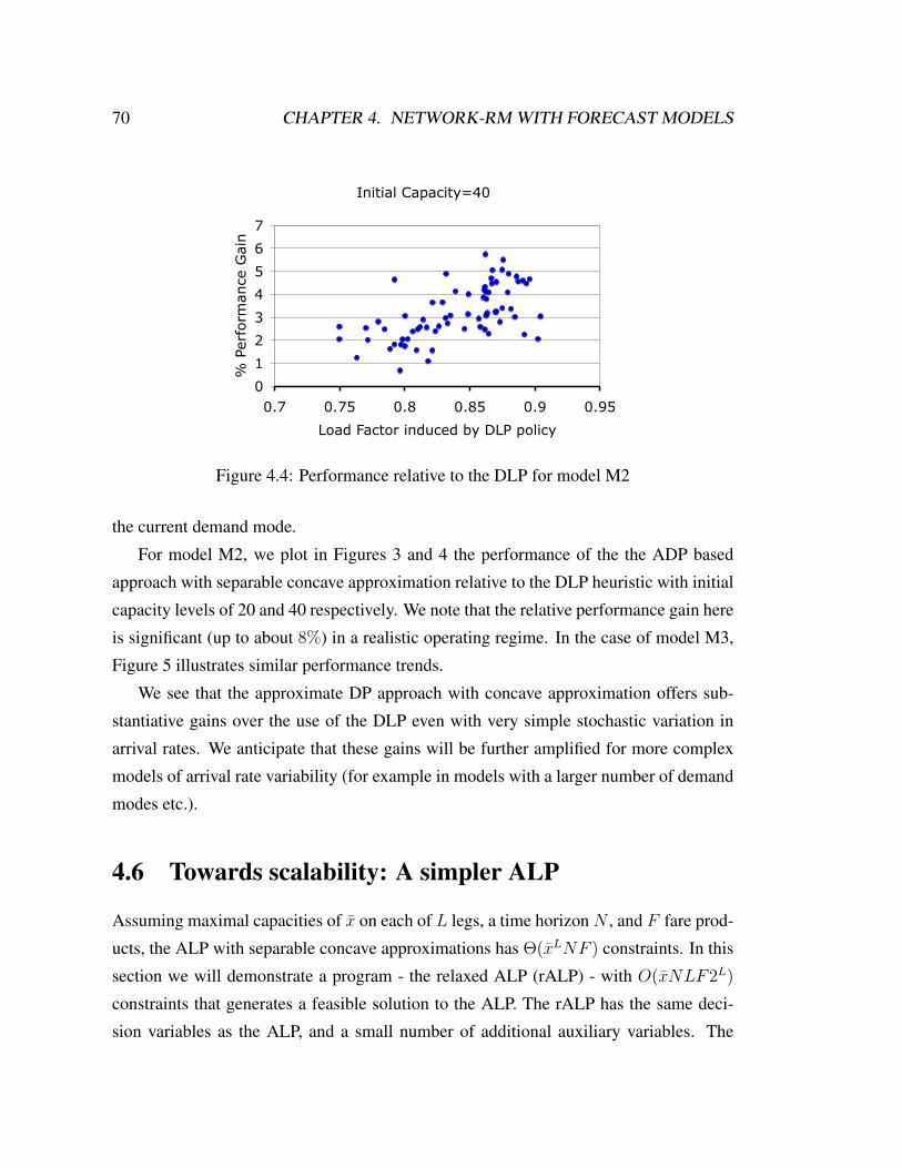
70 CHAPTER 4. NETWORK-RM WITH FORECAST MODELS
Initial Capacity=40
0
1
2
3
4
5
6
7
0.7 0.75 0.8 0.85 0.9 0.95
Load Factor induced by DLP policy
% P
erf
orm
ance G
ain
Figure 4.4: Performance relative to the DLP for model M2
the current demand mode.
For model M2, we plot in Figures 3 and 4 the performance of the the ADP based
approach with separable concave approximation relative to the DLP heuristic with initial
capacity levels of 20 and 40 respectively. We note that the relative performance gain here
is significant (up to about 8%) in a realistic operating regime. In the case of model M3,
Figure 5 illustrates similar performance trends.
We see that the approximate DP approach with concave approximation offers sub-
stantiative gains over the use of the DLP even with very simple stochastic variation in
arrival rates. We anticipate that these gains will be further amplified for more complex
models of arrival rate variability (for example in models with a larger number of demand
modes etc.).
4.6 Towards scalability: A simpler ALP
Assuming maximal capacities of x on each of L legs, a time horizon N , and F fare prod-
ucts, the ALP with separable concave approximations has Θ(xLNF ) constraints. In this
section we will demonstrate a program - the relaxed ALP (rALP) - with O(xNLF2L)
constraints that generates a feasible solution to the ALP. The rALP has the same deci-
sion variables as the ALP, and a small number of additional auxiliary variables. The

4.6. TOWARDS SCALABILITY: A SIMPLER ALP 71
Initial Capacity=20
0
1
2
3
4
5
6
7
8
9
0.75 0.8 0.85 0.9 0.95
Load Factor induced by DLP policy
% P
erf
orm
ance G
ain
Figure 4.5: Performance relative to the DLP for model M3
rALP is consequently a significantly simpler program than the ALP. In the case of affine
approximation, the rALP generates the optimal solution to the ALP. In the case of sepa-
rable concave approximations, the rALP generates a feasible solution to the ALP whose
quality we demonstrate through computational experiments to be excellent. The rALP
solution in fact coincides with the ALP solution in all of our experiments. Our presen-
tation will assume that an itinerary can consist of at most 2 flight legs and will be in
the context of model M1 for simplicity; extending the program to more general arrival
process model is straightforward.
4.6.1 The rALP
In what follows, we understand that for a state s ∈ S, s ≡ (x(s), n(s)). Let us partition
S into sets of the form Sy = {s : s ∈ S, x(s)i = 0 ⇐⇒ yi = 0} for all y ∈ {0, 1}L.
Clearly, S can be expressed as the disjoint union of all such sets Sy. Also define the
subset of fare products Fy according to Fy = {f : Af ≤ y} and assume Fy 6= ∅ for all
y. For some y ∈ {0, 1}L, consider the set of constraints
(TΦr)(s) ≤ (Φr)(s) for all s ∈ Sy. (4.2)

72 CHAPTER 4. NETWORK-RM WITH FORECAST MODELS
We will approximate the feasible region specified by this set of constraints by the follow-
ing set of constraints in r and the auxiliary variables m:
LPy,n(r,m) ≤ 0 ∀n < N
mfl,n,i ≥ rl,n,i ∀ l, n ≤ N, i ∈ {1, . . . , x}, f ∈ Fy∑l:Al,f=1m
fl,n,x ≥ pf ∀n ≤ N, f ∈ Fy
mfl,n,i+1 ≤ mf
l,n,i ∀l, n ≤ N, i ∈ {1, . . . , x− 1}, f ∈ Fy
(4.3)
whereLPy,n(r,m) refers to a certain linear program with decision variables x ∈ RLN(x+1).
We will now proceed to describe this linear program as also discuss how the constraint
LPy,n(r,m) ≤ 0 may itself be described by a set of linear constraints in r,m and certain
additional auxiliary variables.
Let us define:
cy,n(r,m)′x =∑
l
x∑i=0
(rl,n+1,i − rl,n,i)xl,n,i +
∑f∈Fy
λf
∑l:Al,f=1
(x−1∑i=1
(mfl,n+1,i − rl,n+1,i)(xl,n,i − xl,n,i+1) + (mf
l,n+1,x − rl,n+1,x)xl,n,x
)
Implicit in this definition, the vector cy,n(r,m) has components that are themselves linear
functions of r and m. Delaying a precise description for a moment, our goal is to employ
the approximation
∑l:Al,f=1
mfl,n,xl
∼ max((Φr)(x, n)− (Φr)(x− Af , t), pf ),
for all f ∈ Fy, so that cy,n(r,m)′xwill serve as our approximation to (TΦr)(s)−(Φr)(s)
when s ∈ Sy, n(s) = n and x(s)l =∑
i xl,n,i.
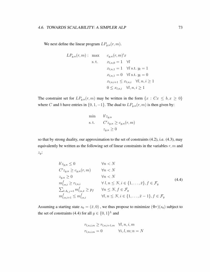
4.6. TOWARDS SCALABILITY: A SIMPLER ALP 73
We next define the linear program LPy,n(r,m).
LPy,n(r,m) : max cy,n(r,m)′x
s. t. xl,n,0 = 1 ∀lxl,n,1 = 1 ∀l s.t. yl = 1
xl,n,1 = 0 ∀l s.t. yl = 0
xl,n,i+1 ≤ xl,n,i ∀l, n, i ≥ 1
0 ≤ xl,n,i ∀l, n, i ≥ 1
The constraint set for LPy,n(r,m) may be written in the form {x : Cx ≤ b, x ≥ 0}where C and b have entries in {0, 1,−1}. The dual to LPy,n(r,m) is then given by:
min b′zy,n
s. t. C ′zy,n ≥ cy,n(r,m)
zy,n ≥ 0
so that by strong duality, our approximation to the set of constraints (4.2), i.e. (4.3), may
equivalently be written as the following set of linear constraints in the variables r,m and
zy:
b′zy,n ≤ 0 ∀n < N
C ′zy,n ≥ cy,n(r,m) ∀n < N
zy,n ≥ 0 ∀n < N
mfl,n,i ≥ rl,n,i ∀ l, n ≤ N, i ∈ {1, . . . , x}, f ∈ Fy∑l:Al,f=1m
fl,n,x ≥ pf ∀n ≤ N, f ∈ Fy
mfl,n,i+1 ≤ mf
l,n,i ∀l, n ≤ N, i ∈ {1, . . . , x− 1}, f ∈ Fy
(4.4)
Assuming a starting state s0 = (x, 0) , we thus propose to minimize (Φr)(s0) subject to
the set of constraints (4.4) for all y ∈ {0, 1}L and
rl,n,i,m ≥ rl,n,i+1,m ∀l, n, i,mrl,n,i,m = 0 ∀i, l,m;n = N

74 CHAPTER 4. NETWORK-RM WITH FORECAST MODELS
in order to compute our approximation to the value function. We will refer to this pro-
gram as rALP (s0).
4.6.2 Quality of Approximation
We have proposed approximating the feasible region specified by the set of constraints
(TΦr)(s) ≤ (Φr)(s) for all s ∈ S
which has size that is Θ(xLNF ) by a set of linear constraints of sizeO(xNLF2L). There
are two potential sources of error for this approximation: For one, we would ideally like
to enforce the constraint cy,n(r,m)′x ≤ 0 only for x·,n,· in {0, 1}(x+1)L, whereas in fact
we allow x·,n,· to take values in [0, 1](x+1)L. It turns out that this relaxation introduces
no error to the approximation, simply because the vertices of LPy,n(r,m) are integral.
That is, the optimal solutions always satisfy x∗l,n,i ∈ {0, 1}. This is simple to verify;
LPy,n(r,m) may be rewritten as a min-cost flow problem on a certain graph with integral
supplies at the sources and sinks.
The second source of approximation error arises from the fact that we approximate
max((Φr)(x, n)− (Φr)(x− Af , n), pf ) by∑
l:Al,f=1mfl,n,xl
. In particular, we have:
∑l:Al,f=1
mfl,n(s),x(s)l
≥ max((Φr)(s)− (Φr)(x(s)− Af , n(s)), pf ) (4.5)
This yields the following Lemma. A proof may be found in the appendix.
Lemma 12. rALP (s0) ≥ ALP (s0). Moreover if (rrALP ,m) is a feasible solution to the
rALP then rrALP is a feasible solution to the ALP.
In the case of affine approximations the reverse is true as well. That is, we have:
Lemma 13. For affine approximations, rALP (s0) ≤ ALP (s0). Moreover if rALP is a
feasible solution to the ALP then there exists a feasible solution to the rALP, (rrALP ,m)
satisfying rrALP = rALP .
Consequently, the rALP yields the optimal solution to the ALP for affine approxima-
tions. In the case of separable concave approximations, the rALP will in general yield

4.6. TOWARDS SCALABILITY: A SIMPLER ALP 75
suboptimal solutions to the ALP. One may however show that there exists an optimal
solution to the rALP satisfying for all s ∈ S:
∑l:Al,f=1
m∗,fl,n(s),x(s)l
≥ max((Φr∗)(s)−(Φr∗)(x(s)−Af , n(s)), pf ) ≥1
2
∑l:Al,f=1
m∗,fl,n(s),x(s)l
,
(4.6)
so that heuristically we might expect the rALP to provide solutions to the ALP that are
of reasonable quality. In fact, as our computational experiments in the next subsection
illustrate, the rALP appears to yield the optimal ALP solution in the case of separable
concave approximations as well.
4.6.3 Computational experience with the rALP
We consider problems with 3, 4, and 8 flights with problem data generated as in the
computational experiments in Section 5. Table 1 illustrates the solution objective and
solution time for the rALP and ALP for each of these problems. For the 3 and 4 dimen-
sional problems, we consider instances small enough so that it is possible to solve the
ALP exactly. We see in these instances that the rALP delivers the same solution as the
ALP in a far shorter time. The ALP for the 8 dimensional instance cannot be stored - let
alone solved - on most conventional computers; the rALP for that problem on the other
hand is relatively easy to solve and yields a near optimal solution (the comparison here
being with the optimal solution of an RLP with 100,000 sampled constraints; recall that
the RLP solution is a lower bound on the ALP).
In practice we envision the rALP being used in conjunction with constraint sampling.
In particular, consider the following alternative to the RLP of Section 4: Let X be the
set of sampled states one might use for the RLP. We then include in the rALP the set of
constraints (4.3) for only those (y, n) such that there exists a sampled state (x, n) ∈ Xwith x(s) ∈ Sy. The sampled rALP will haveO(xLFK(X )) constraints whereK(X ) =
|{(y, n) : ∃s ∈ X s.t. s ∈ Sy, n(s) = n}|. Since a majority of sampled states are likely to
be in Se where e is the vector of all ones (indicating that all fare products can potentially
be serviced), one may expect K(X ) to be far smaller than |X |, making the sampled
rALP a significantly simpler program than the RLP. Moreover, since the sampled rALP

76 CHAPTER 4. NETWORK-RM WITH FORECAST MODELS
Dimension x T ALP (s0) rALP (s0) tALP trALP
310 50 925.46 925.46 99.33 2.67420 50 1035.23 1035.23 2611.89 11.46
410 10 218.28 218.28 161.67 0.4110 30 653.37 653.37 2771.0 2.45
810 100 5019.90∗ 5028.15 849.2∗ 1251.9210 100 5019.90∗ 5028.12∗∗ 849.2∗ 177.77 ∗∗
Table 4.1: Solution quality and computation time for the rALP and ALP. * indicatesvalues for an RLP with 100,000 constraints (recall that the RLP provides a lower boundon the ALP). ** indicates values for the sampled rALP described in section 6.3 using thesame sample set as that in the computation of the corresponding RLP. Computation timereported in seconds for the CPLEX barrier LP optimizer running on a workstation witha 64 bit AMD processor and 8GB of RAM.
attempts to enforce (TΦr)(s) ≤ (Φr)(s) for a collection states that are a superset of the
states in X , we might expect it to provide a stronger approximation as well. While a
thorough exploration of the sampled rALP is beyond the scope of this chapter, the last
row of Table 1 provides encouraging supporting evidence.
4.7 Discussion and Conclusions
We have explored the use of separable concave functions for the approximation of the
optimal value function for the dynamic capacity allocation problem. The approximation
architecture is quite flexible and we have illustrated how it might be employed in the con-
text of a general arrival process model wherein arrival rates vary stochastically according
to a Markov process. Our computational experiments indicate that the use of the LP
approach to Approximate DP along with this approximation architecture can yield sig-
nificant performance gains over the DLP (of up to about 8%) , even when re-computation
of DLP bid prices is allowed at every time step. Moreover, our control policy is a bid
price policy where policy execution requires a table look-up at each epoch making the
methodology ideally suited to real time implementation. State of the art heuristics for the
dynamic capacity allocation problem typically resort to using point estimates of demand
in conjunction with a model that assumes simple time homogeneous arrival processes in

4.7. DISCUSSION AND CONCLUSIONS 77
order to make capacity allocation decisions dynamically. As such, our algorithm may
be viewed as a viable approach to moving beyond the use of point estimates and instead
integrating forecasting and optimization. The approach we propose is also scalable. For
example, the sampled rALP proposed in section 6 may be solved in a few minutes for
quite large problems.
Our approximate DP approach offered only a marginal performance improvement
relative to the DLP in the case where demand for the various fare classes were time
homogenous Poisson processes. In fact, the DLP is asymptotically optimal for such
demand processes (when one scales the time horizon T and the starting inventory level
x0). This is not surprising, and is essentially the consequence of an averaging effect: in
particular, if demand for a fare class is a Poisson processes, then expected demand for that
fare class is Θ(T ) (in the time horizon T ), and realized demand is with high probability
within an additive factor of Θ(√T ) of expected demand. Of course, the Poisson process
is not unique in this regard, and the DLP is likely to yield close to optimal performance if
demand for fare classes demonstrates averaging behavior of this manner on a time-scale
comparable to the sales horizon T . Demand in models M1 and M2 (for which we show
a significant improvement over the DLP) does not demonstrate this averaging effect due
to a random transition in arrival rates at ∼ T/2. In summary, we note that if demand for
fare classes is likely to experience significant shocks on a time scale that is slow relative
to the time horizon, the DLP is unlikely to be near optimal and our approximate DP
methods are likely to yield significant improvements.
Several issues remain to be resolved. For example, in the interest of very large-
scale implementations, it would be useful to explore the use of simpler basis functions
that are nonetheless capable of capturing the concavity of the true value function. In
computational experiments, the rALP produced optimal solutions to the ALP; it would be
interesting to establish that the programs are equivalent (as we have in the case of affine
approximations). The ALP produces a tighter approximation to the true value function
than does the DLP but it remains to show that the ALP policy dominates the DLP policy
as well if this is at all true. Finally, a computational exploration of our approach with a
highly realistic simulator such as that used by P.P.Belobaba (2001) would give a better
sense for the gains that one may hope to achieve via the use of this approach in practice.

Concluding Remarks
The “estimate, then optimize” paradigm is widely used in practice. Its use stems primar-
ily from the speed and modularity requirement for modern RM systems. Yet, it is not
without its flaws. This thesis set out to address some of those flaws. In particular, we
asked two questions:
• Would addressing these flaws produce a tangible impact on revenues?
• Could these flaws be addressed in a manner that is robust and efficient?
While definitive answers to either question can only be provided through real world
tests and implementations, we have over the course of this thesis provided support for af-
firmative answers to both. In particular, we saw that accounting for the incentive to learn
(in the case of the one product dynamic pricing problem) and optimization that attempts
to harness all the predictive capabilities of a forecast model (for problems of network-
RM), could potentially yield large performance gains. This perhaps isn’t so surprising.
What is noteworthy is that we were able to accomplish these goals via tractable schemes
that required no more computational effort than existing approaches to these problems.
RM optimization research has typically focused on highly simplified models of cus-
tomer demand. In part this is because there is a dearth of information on “true” demand
models used in practice (these are highly proprietary), and in part because many of these
optimization problems are hard in spite of such simplifying assumptions. Hopefully, the
insights we have gained through this study encourage the use of optimization techniques
that attempt to incorporate more realistic models of demand.
78

Appendix A
Proofs for Chapter 2
A.1 Proofs of Theorems 1 and 2
A.1.1 Existence of Solutions to the HJB Equation
Our proofs to both Theorems 1 and 2 will rely on showing the existence of a bounded
solution to the HJB Equation (HJ)(z) = 0 for z ∈ Sx,a,b. We will demonstrate the
existence of a solution to the HJB Equation wherein price is restricted to some bounded
interval. We will later show that the solution obtained is in fact a solution to the original
HJB Equation.
Define B = r + rb
(1 + e−1(a+x)
aα+ e−1(a+x)
α
). Let ΠB be the set of admissible price
functions bounded by B, and define the Dynamic programming operator
(HBJ)(z) = supπ∈ΠB
(HπJ)(z)
We will first illustrate the existence of a bounded solution to the HJB Equation:
(HBJ)(z) = 0 (A.1)
for z ∈ Sx,a,b.
For some arbitrary N > b let us first construct a solution on the compact set SNx,a,b
≡{(x, a, b) ∈ S : x+a = x+ a; b ≤ b ≤ N} with the boundary conditions J(x, a,N) = 0
79

80 APPENDIX A. PROOFS FOR CHAPTER 2
and J(0, a, b) = 0.
Lemma 14. (A.1) has a unique bounded solution on SNx,a,b
satisfying J(x, a,N) = 0 and
J(0, a, b) = 0.
In the interest of brevity, the proof to the Lemma is omitted. Nonetheless, we provide
a sketch: Upon setting J(0, a, b) = 0, (A.1) can be interpreted as an initial value problem
of the form J = f(J, b) with J(N) = 0, in the space Rx−1 equipped with the max-
norm. It is then routine to check the requirements for the application of a local existence
Theorem for ODE’s in a Banach space (such as Theorem 11.19 in Jost (2000)).
The following two Lemma’s construct a solution to (A.1) on Sx,a,b using solutions
constructed on SNx,a,b
.
Lemma 15. Let JN be the unique solution to (A.1) on SNx,a,b
with J(x, a,N) = 0 and
J(0, a, b) = 0. Moreover, let JN ′be the unique solution to (A.1) on SN ′
x,a,bfor some
N ′ > N with J(x, a,N ′) = 0 and J(0, a, b) = 0. Then, for (x, a, b) ∈ SNx,a,b
,
|JN(x, a, b)− JN ′(x, a, b)| ≤ r
a+ x
bexp(−α(N − b))
Moreover, JN(x, a, b) ≤ re−1(a+x)
αb
Proof: Define τN = inf{t : nt = x} ∧ inf{t : bt = N}. Similarly, define τN ′ . Let
π∗,N(·), defined on SNx,a,b
, be the greedy price with respect to JN . Finally, define the
“revenue” function r∗,Nt =ate
−π∗,Nt /rπ∗,N
t
bt. We then have, via an application of Lemma 4,
JN(x, a, b) = Ez,π∗,N
[∫ τN
0
e−αtr∗,Nt dt
]+ Ez,π∗,N
[e−ατNJN(xτN
, aτN, bτN
)]
= Ez,π∗,N
[∫ τN
0
e−αtr∗,Nt dt
]Note that this immediately yields:
JN(x, a, b) ≤ J∗(x, a, b) ≤ J∗a/b(x) ≤re−1(a+ x)
αb.

A.1. PROOFS OF THEOREMS 1 AND 2 81
Now, for an arbitrary π ∈ ΠB, and the corresponding revenue function r, we have (again,
via Lemma 4)
JN ′(x, a, b) ≥ Ez,π
[∫ τN′
0
e−αtrtdt
]+ Ez,π
[e−ατN′JN ′
(xτN′ , aτN′ , bτN′ )]
= Ez,π
[∫ τN′
0
e−αtrtdt
]In particular, using the price function π = π∗,N for b ≤ N and 0 otherwise, yields,
JN ′(x, a, b) ≥ Ez,π∗,N
[∫ τN
0
e−αtr∗,Nt dt
]= JN(x, a, b) (A.2)
The same argument, applied to JN , with the price function π∗,N ′ , yields
Ez,π∗,N′
[∫ τN
0
e−αtr∗,N′
t dt
]≤ JN(x, a, b)
Finally, noting that on {τN ′ > τN}, τN ≥ N − b, we have
Ez,π∗,N′
[∫ τN′
τN
e−αtr∗,N′
t dt
]≤ r
a+ x
bexp(−α(N − b))
Adding the two preceding inequalities, yields
JN ′(x, a, b)− r
a+ x
bexp(−α(N − b)) ≤ JN(x, a, b).
Since JN ′(x, a, b) ≥ JN(x, a, b) by (A.2), the result follows.
2
Lemma 16. limN→∞ JN exists on Sx,a,b, is bounded, and solves system (A.1)
The key step here is showing limNddbJN = d
dblimN J
N for all z ∈ Sx,a,b; this is
routine analysis given the result of the preceding Lemma and is omitted for brevity. The
previous Lemma constructs a bounded solution to (A.1). We now show that this solution
is in fact a solution to the original HJB Equation (HJ)(z) = 0 for z ∈ Sx,a,b.

82 APPENDIX A. PROOFS FOR CHAPTER 2
Lemma 17. Let J be a bounded solution to (A.1). Then, J is a solution to (HJ)(z) = 0
for z ∈ Sx,a,b.
Proof: We show the claim by demonstrating that the greedy price (in ΠB) with respect
to J is in fact attained in [0, B). We begin by proving a bound on such a greedy price.
Let πdb ∈ ΠB be the greedy price with respect to J , and τ = inf{t : Nt = x0}. We have,
via Lemma 4,
J(z) = Ez,πdb
[∫ τ
0
e−αtrtdt
]+ Ez,πdb
[e−ατ J(zτ )
]= Ez,πdb
[∫ τ
0
e−αtrtdt
]≤ J∗(z)
≤ re−1(a+ x)
αb.
Now let Jδ be the solution to (A.1) when the discount factor is α(1 + δ/b). Let πδdb be
the corresponding greedy price. We then have from Lemma 4 and using the fact that
J(x, a, b+ δ) = Jδ(x, a, b),
J(x, a, b+ δ) = Ez,πδdb
[∫ τ
0
e−α(1+δ/b)trδtdt
]≥ Ez,πdb
[∫ τ
0
e−α(1+δ/b)trtdt
]It follows that
J(z)− J(x, a, b+ δ) ≤ Ez,πdb
[∫ τ
0
(e−αt − e−α(1+δ/b)t)rtdt
]≤∫ ∞
0
(e−αt − e−α(1+δ/b)t)re−1(a+ x)
bdt
so thatd
dbJ(z) ≥ −rα
b
e−1(a+ x)
bα2

A.1. PROOFS OF THEOREMS 1 AND 2 83
Putting the two bounds together yields
J(x− 1, a+ 1, b)− J(z) +b
a
d
dbJ(z) ≥ −re
−1(a+ x)
αb− re−1(a+ x)
abα(A.3)
Now observe that the greedy price πdb ∈ Π with respect to J is given by
p =
(r − J(x− 1, a+ 1, b) + J(z)− b
a
d
dbJ(z)
)+
which by (A.3) is in [0, B), so that we have that J is, in fact, a solution to (HJ)(z) = 0
for z ∈ Sx,a,b. 2
A.1.2 Proofs for Theorems 1 and 2
Lemma 18.
Aπ,zJ(z) = e−π(z)/r a
b
(J(z′)− J(z) +
b
a
d
dbJ(z)
)− αJ(z)
Proof: As in Theorem T1 in Section VII.2 of Bremaud (1981), one may show for
J ∈ J , and an arbitrary z0 ∈ Sx,a,b,
J(zt) =J(z0) +
∫ t
0
[b
a
d
dbJ(zs) + J(xs − 1, as + 1, bs)− J(zs)
]as
bse−ps/rds
+
∫ t
0
[J(xs− − 1, as− + 1, bs−)− J(zs−)] (dNs −as
bse−ps/rds)
It is not hard to show that that Ns− as
bse−ps/r is a zero-mean σ(zs, ps) martingale, so that
we may conclude
e−αtE[J(zt)]− J(z0) =
e−αtE
[∫ t
0
[d
dbJ(zs) + J(xs − 1, as + 1, bs)− J(zs)
]as
bse−ps/rds
]+ (e−αt − 1)J(z0)
Dividing by t and taking a limit as t→0 yields, via bounded convergence, the result. 2

84 APPENDIX A. PROOFS FOR CHAPTER 2
Lemma 19. (Verification Lemma) If there exists a solution, J ∈ J to
(HJ)(z) = 0
for all z ∈ Sx,a,b, we have:
1. J(·) = J∗(·)
2. Let π∗(·) be the greedy policy with respect to J . Then π∗(·) is an optimal policy.
Proof:Let π ∈ Π be arbitrary. By Lemma 4
Jπ(z0)− J(z0) =E
[∫ τ0
0
e−αsHπJ(zs)ds
]≤0
(A.4)
with equality for π∗(·), since Hπ∗ J(z) = (HJ)(z) = 0 for all z ∈ Sx,a,b. 2
Now we have shown the existence of a bounded solution, J to (HJ)(z) = 0 on Sx,a,b
in the previous section, so that the first conclusion of the Verification Lemma gives
Theorem 1. The value function J∗ is the unique solution in J to HJ = 0.
The second conclusion and (A.4) in the Verification Lemma give
Theorem 2. A policy π ∈ Π is optimal if and only if HπJ∗ = 0.
A.2 Proofs for Section 2.5
Lemma 1. For all z ∈ S, α > 0
J∗(z) ≤ J(z) ≤ J∗µ(z)(x) ≤F (p∗)p∗µ(z)
α.
where p∗ is the static revenue maximizing price.

A.3. PROOFS FOR SECTION 2.7 85
Proof: We begin with showing that J∗λ(·) is concave in λ. Consider maximizing the
sum of revenues from two independent systems, both of which have an initial inventory
x and arrival rates λ1 and λ2 respectively. It is clear that the revenue maximizing policy
is one which charges π∗λ1(x1(t)) in the λ1 system and π∗λ2
(x2(t)) in the λ2 system. Now
consider a system with no inventory constraint that at every time t must post a price
for both the λ1 and λ2 streams, but registers sales and receives revenues from only one
of the streams (w.p. 1/2 for each). The system cannot register any sales after a total
of 2x sales (both registered and unregistered) have occurred. Note that irrespective of
the policy employed the system will register X sales where X is a Binomial(2x, 1/2)
random variable. Moreover it is possible to show that givenX , one may generate arrivals
so that the relevant arrival stream continues to be Poisson((λ1 +λ2)/2. Consider a policy
that charges π∗λ1(x1(t)) in the λ1 system and π∗λ2
(x2(t)) in the λ2 system. The expected
revenue under such a policy is precisely (J∗λ1(x)+J∗λ2
(x))/2. Moreover, it is clear that the
expected revenue for such a system under the optimal policy is E[J∗(λ1+λ2)/2(X)] where
X is a Binomial(2x, 1/2) random variable. A simple induction using the monotonicity of
the Hλ operator establishes that J∗λ(x)−J∗λ(x−1) is non-increasing in x so that we have
by Jensen’s inequality that E[J∗(λ1+λ2)/2(X)] ≤ J∗(λ1+λ2)/2(x). The concavity of J∗λ(·) in
λ follows.
Now since J∗λ(x) is concave in λ, Jensen’s inequality gives us that J∗a/b(x) = J∗E[λ](x) ≥E[J∗λ(x)] = J(z). Note that J∗λ(x) is bounded above by the value of a system with cus-
tomer arrival rate λ but without a finite capacity constraint. The optimal policy in such a
system is simply to charge the static revenue maximizing price, p∗, garnering a value ofF (p∗)p∗λ
αyielding J∗λ(x) ≤ F (p∗)p∗λ
α. 2
A.3 Proofs for Section 2.7
Lemma 3. For all z ∈ S, α > 0, J∗,α(z) = J∗,1(x, a, αb).
Proof: Consider the following coupling of the α system starting at state (x, a, b), and of
the 1 system starting at state (x, a, αb). Let us assume that the first system is controlled by
the price function π1(·) while the second is controlled by the price function π2(·) where
π2(x, a, b) = π1(x, a, b/α). Consider the evolution of system 1 under a sample path with

86 APPENDIX A. PROOFS FOR CHAPTER 2
arrivals at {tk} and a corresponding binary valued sequence {ψk} and of system 2 with
arrivals {t′k} = {αtk} and the same binary valued sequence {ψk}. Now let {tk , k ≤ x}be distributed as the first x points of a Poisson(λ) process where λ ∼ Γ(a, b). Then it
is easy to verify that {αtk , k ≤ x} is distributed as the first x points of a Poisson(λ)
process where λ ∼ Γ(a.αb). It immediately follows that:
Jπ1,α(x, a, b) = Eλ∼Γ(a.b)
[x∑
k=1
ψkπ1(t−k ) exp(−α(tk))
]
= Eλ∼Γ(a.b)
[x∑
k=1
ψkπ2(αt−k ) exp(−(αtk))
]
= Eλ∼Γ(a.αb)
[x∑
k=1
ψkπ2(t−k ) exp(−tk)
]= Jπ2,1(x, a, αb)
The result follows by taking a supremum over all price functions π1. 2
Lemma 4. Let J ∈ J satisfy J(0, a, b) = 0. Let τ = inf{t : J(zt) = 0}. Let z0 ∈ Sx,a,b.
Then,
E
[∫ τ
0
e−αtHπJ(zt)dt
]= Jπ(z0)− J(z0)
Let J : N → R be bounded and satisfy J(0) = 0. Let τ = inf{t : J(xt) = 0}. Let
x0 ∈ N. Then,
E
[∫ τ
0
e−αtHπλJ(xt)dt
]= Jπ
λ (x0)− J(x0)
Proof: Define for J ∈ J , and π ∈ Π,
Aπ,zJ(z) = limt>0,t→0
=e−αtEz,π[J(z(t))]− J(z)
t
Define
HπJ(z) = F (π(z))a
bπ(z) +Aπ,zJ(z)

A.3. PROOFS FOR SECTION 2.7 87
Lemma 18 verifies that this definition is in agreement with our previous definition pro-
vided J ∈ J . Let τ be a stopping time of the filtration σ(zt). We then have:
E
[∫ τ
0
e−αtHπJ(zt)dt
]= E
[∫ τ
0
e−αt(F (π(zt))
a
bπ(zt) +Aπ,zJ(zt)
)dt
]= Jπ(z0) + Ez0
[e−ατJ(zτ )
]− J(z0)
= Jπ(z0)− J(z0)
where the second equality follows from Dynkin’s formula. The proof of the second
statement is analogous. 2
Lemma 5. If λ < µ, Jπnl
λ (x) ≥ λ/µJ∗µ(x) for all x ∈ N.
Proof: Letting τ = inf{t : nt = x0} as usual, we have
−E[∫ τ
0
e−αtHπnl
λ J∗ρ (xt)dt
]= E
[∫ τ
0
e−αt(1− λ/ρ)αJ∗ρ (xt)dt
]≤ E
[∫ τ
0
e−αt(1− λ/ρ)αJ∗ρ (x0)dt
]≤ (1− λ/ρ)J∗ρ (x0)
where the inequality follows from the fact that J∗ρ (x) is decreasing in x and since λ < ρ
here. So, from Lemma 4, we immediately have:
J∗ρ (x0)− Jπnl
λ (x0) ≤ (1− λ/ρ)J∗ρ (x0)
which is the result. 2
Lemma 6. If λ ≥ µ, Jπnl
λ (x) ≥ J∗µ(x) for all x ∈ N.
Proof: Here,
−E[∫ τ
0
e−αtHJ∗π0(x(t))dt
]≤ 0
so the result follows immediately from Lemma 4. 2
Corollary 1. For all z ∈ S , and reservation price distributions satisfying Assumptions 1

88 APPENDIX A. PROOFS FOR CHAPTER 2
and 21
κ(a)≤ πdb(z)
π∗(z)≤ 1
Proof: Recall that the decay balance equation implies that F (p∗)p∗ρ(π∗(z))
F (π∗(z))= F (p∗)p∗a
J∗(z)bα=
r∗. Let F (p∗)p∗(a/bα)
J(z)= r. Lemma 1 implies that r∗ ≥ r ≥ 1. It is simple to check that
when the right hand side is 1, the equation is satisfied uniquely by p = p∗, the static
revenue maximizing price. Now we have that πdb(z) = p∗+ πdb(z)−p∗
r−1(r− 1) and by part
1 of Assumption 2, π∗(z) ≤ p∗ + πdb(z)−p∗
r−1(r∗ − 1). Consequently,
πdb(z)
π∗(z)≥
p∗ + πdb(z)−p∗
r−1(r − 1)
p∗ + πdb(z)−p∗
r−1(r∗ − 1)
≥p∗ + πdb(z)−p∗
r−1(r − 1)
p∗ + πdb(z)−p∗
r−1(κ(a)r − 1)
≥p∗ + (r − 1)/(F (p∗)p∗ d
dpρ(p)
F (p)
∣∣p=p∗
)
p∗ + (κ(a)r − 1)/(F (p∗)p∗ ddp
ρ(p)
F (p)
∣∣p=p∗
)
≥ 1
κ(a)
where the second inequality follows from Theorem 3, the third inequality follows from
the convexity assumed in part 1 of Assumption 2, and the final inequality follows from
part 2 of Assumption 2. The upper bound is immediate from the fact that J∗(z) ≤ J(z).
2
Lemma 7. For all z ∈ S, and reservation price distributions satisfying Assumptions 1
and 2,
Jub(z) ≥ J∗(z)
Proof: Define the operator:
(HubJ)(z) = F (πdb(z))
(a
b(π∗(z) + J(z′)− J(z)) +
d
dbJ(z)
)− e−1J(z).
Analogous to the proof of Theorem 1, one may verify that Jub is the unique bounded
solution to (HubJ)(z) = 0 for all z ∈ Sx,a,b satisfying Jub(0, a, b) = 0. Identically to the

A.3. PROOFS FOR SECTION 2.7 89
proof of Lemma 4, we can then show for J ∈ J satisfying J(0, a, b) = 0, and z0 ∈ Sx,a,b
that
E
[∫ τ
0
e−αtHubJ(zt)dt
]= Jub(z0)− J(z0) (A.5)
Now, observe that for x > 0,
(HubJ∗)(z)
= F (πdb(z))
(a
b(π∗(z) + J∗(z′)− J∗(z)) +
d
dbJ∗(z)
)− e−1J∗(z)
≥ F (π∗(z))
(a
b(π∗(z) + J∗(z′)− J∗(z)) +
d
dbJ∗(z)
)− e−1J∗(z)
= 0
where for the inequality, we use the fact that
π∗(z) + J∗(z′)− J∗(z) +b
a
d
dbJ∗(z) = 1/ρ(π∗(z)) ≥ 0
and that πdb(z) ≤ π∗(z) from Corollary 1. The equality is simply Theorem 1. We
consequently have
HubJ∗(z) ≥ 0 ∀z ∈ Sx,a,b
so that (A.5) applied to J∗ immediately gives:
Jub(x, a, b) ≥ J∗(x, a, b)
2
Lemma 8. For all z ∈ S, r > 0, J∗,r(z) = rJ∗,1(z).
Proof: Consider the following coupling of the r system starting at state z = (x, a, b),
and of the 1 system starting at state z. Let us assume that the first system is controlled
by the price function π1(·) while the second is controlled by the price function π2(·) =
(1/r)π1(·). Consider the evolution of both systems under a sample path with arrivals
at {tk} and a corresponding binary valued sequence {ψk} indicating whether or not the
consumer chose to make a purchase. Let E[·] be a joint expectation over {tk, ψk; k ≤ x}

90 APPENDIX A. PROOFS FOR CHAPTER 2
assuming {tk} are the points of a Poisson(λ) process where λ ∼ Γ(a, b), and ψk is a
Bernoulli random variable with parameter exp(−π1(t−k )/r) = exp(−π2(t
−k )). We then
have:
Jπ1,r(z) = E
[x∑
k=1
ψkπ1(t−k ) exp(−α(tk))
]
= rE
[x∑
k=1
ψkπ2(t−k ) exp(−α(tk))
]= rJπ2,1(z)
The result follows by taking a supremum over all price functions π1. 2
Lemma 9. For all z ∈ S ,
J∗(z|τ) ≤
e−e−1τ(e−(π∗−πdb)
[π∗ + J∗(x− 1, a+ 1, bdb
τ )]+ (1− e−(π∗−πdb))J∗(x, a+ 1, bdb
τ ))
where π∗ = π∗(x, a, b∗τ ) and πdb = πdb(x, a, bdbτ ).
Proof: Define Fdbt = σ(zdb
t ) and F∗t = σ(z∗t ) Then,
J∗(z|τ)
= E
[x∑
k=1
e−e−1tkπ∗t−k
∣∣∣∣σ(Fdbτ− ∪ F∗
τ−)
]
= E
[x∑
k=1
e−e−1tkπ∗t−k
∣∣∣∣λ|σ(Fdbτ− ∪ F∗
τ−), x
]≤ e−e−1τ
[e−(π∗−πdb)[π∗ + J∗(x− 1, a+ 1, bdb
τ )] + (1− e−(π∗−πdb))J∗(x, a+ 1, bdbτ )]
The second equality is from conditional independence of the past given the distribution
of λ|σ(Fdbt ∪ F∗
t ) and xt. For the third inequality, we note that since π∗(·) ≥ πdb(·),and further since πdb(·) is decreasing in b, we must have that π∗t ≥ πdbt on t < τ .
Consequently, we must have that, b∗t ≤ bdbt , on t < τ , so that, λ|σ(Fdb
τ− ∪ F∗τ−) is a
Gamma random variable with shape parameter a+ 1 and scale parameter, bdbτ so that we

A.3. PROOFS FOR SECTION 2.7 91
have,
E
[x∑
k=1
e−e−1tkπ∗t−k
∣∣∣∣λ|σ(Fdbτ− ∪ F∗
τ−), x
]
≤ sup{π:πt=π∗t on t<τ}
E
[x∑
k=1
e−e−1tkπt−k
∣∣∣∣λ|σ(Fdbτ− ∪ F∗
τ−), x
]
which on {n∗τ = 1} is equal to e−e−1τ (π∗ + J∗(x − 1, a + 1, bdbτ )) and on {n∗τ = 0} is
equal to e−e−1τJ∗(x, a+ 1, bdbτ ). The inequality follows from the fact that π∗ ignores the
information in Fdbτ− . 2
Lemma 10. For x > 1, a > 1, b > 0, J∗(x, a, b) ≤ 2.05J∗(x− 1, a, b).
Proof: Let τ1 = inf{t : n∗(t) = x− 1}, and define
J∗,τ1(z) = Ez,π∗
[x−1∑k=1
e−e−1tkπt−k
].
Now,
J∗(z) = J∗,τ1(z) + E[e−e−1τ1J∗(1, a+ x− 1, bτ1)
](A.6)
We will show that E[e−e−1τ1J∗(1, a+ x− 1, bτ1)
]≤ 1.05J∗(x − 1, a, b). Since we
know by definition that J∗(x−1, a, b) ≥ J∗,τ1(z), the result will then follow immediately
from (A.6).
To show E[e−e−1τ1J∗(1, a+ x− 1, bτ1)
]≤ 1.05J∗(x − 1, a, b), we will first estab-
lish a lower bound on
π∗(2, a+ x− 2, bτ1)/J∗(1, a+ x− 1, bτ1).
Let a+ x− 2 ≡ k, a+ x− 1 ≡ k′. Certainly, k′ ≤ 2k since a > 1. Now,
π∗(2, k, b) = 1 + log k/b− log J∗(2, k, b) ≥ 1 + log k/b− log J∗k/b(2)

92 APPENDIX A. PROOFS FOR CHAPTER 2
and J∗(1, k′, b) ≤ J∗(1, 2k, b) ≤ J∗2k/b(1) so that
π∗(2, k, b)
J∗(1, k′, b)≥ 1 + log k − log J∗k (2)
J∗2k(1)
But,
infk∈(0,∞)
1 + log k − log J∗k (2)
J∗2k(1)= inf
k∈(0,∞)
1 + log k − logW (keW (k))
W (2k)≥ 0.96
so thatπ∗(2, a+ x− 2, bτ1)
J∗(1, a+ x− 1, bτ1)≥ 0.96
It follows that
J∗(x− 1, a, b) ≥ J∗,τ1(z)
≥ E[e−e−1τ1π∗(2, a+ x− 2, bτ1)]
≥ 0.96 E[e−e−1τ1J∗(1, a+ x− 1, bτ1)]
Substituting in (A.6), we have the result. 2

Appendix B
Proofs for Chapter 4
B.1 Proofs for Section 4.4
Lemma 11. For model M2 with initial state s, J∗(s) ≤ ALP (s) ≤ DLP (s)
Proof: We assume for notational convenience that N is even. Consider the following
linear program:
sDLP (s) : max p′z0 + Pr(sN/2 = lo)p′z1 + Pr(sN/2 = hi)p′z2
s. t. A(z0 + z1) ≤ x(s)
A(z0 + z2) ≤ x(s)
0 ≤ z0 ≤ E[D0]− E[DN/2]
0 ≤ z1 ≤ E[DN/2|sN/2 = lo]
0 ≤ z2 ≤ E[DN/2|sN/2 = hi]
It is clear that sDLP (s) ≤ DLP (s). This is because z0 + Pr(sN/2 = lo)z1 + Pr(sN/2 =
hi)z2 is a feasible solution to DLP (s) of the same value as sDLP (s). We will first show
93

94 APPENDIX B. PROOFS FOR CHAPTER 4
that ALP (s) ≤ sDLP (s). The dual to sDLP (s) is given by:
min x(s)′y1,1 + x(s)′y1,2 + D′0y2,0 + D′
1y2,1 + D′2y2,2
s. t. A′(y1,1 + y1,2) + y2,0 ≥ p
A′y1,1 + y2,1 ≥ pPr(sN/2 = lo)
A′y1,2 + y2,2 ≥ pPr(sN/2 = hi)
y1,1, y1,2, y2,0, y2,1, y2,2 ≥ 0
where D0 = E[D0]− E[DN/2], D1 = E[DN/2|sN/2 = lo] and D2 = E[DN/2|sN/2 = hi].
Consider the following solution to the ALP for M2: Set
r∗l,n,i,med
= (y∗1,1)l + (y∗1,2)l
for i > 0, n < N/2
= D′0,ny
∗2,0 + Pr(sN/2 = lo)r∗1,N/2,0,lo + Pr(sN/2 = hi)r∗1,N/2,0,hi
for i = 0, l = 1, n < N/2
= 0 otherwise
r∗l,n,i,lo
= (y∗1,1)l/Pr(sN/2 = lo) for i > 0, N > n ≥ N/2
= D′1,ny
∗2,1/Pr(sN/2 = lo) for i = 0, l = 1, N > n ≥ N/2
= 0 otherwise
r∗l,n,i,hi
= (y∗1,2)l/Pr(sN/2 = hi) for i > 0, N > n ≥ N/2
= D′2,ny
∗2,2/Pr(sN/2 = hi) for i = 0, l = 1, N > n ≥ N/2
= 0 otherwise
where D0,n = E[Dn] − E[DN/2] for n < N/2, D1,n = E[Dn|sN/2 = lo] and D2,n =
E[Dn|sN/2 = hi] for n ≥ N/2. It is routinely verified that this solution is in fact feasible
for the ALP and has value equal to sDLP (s). The fact that ALP (s) ≥ J∗(s) follows
from the monotonicity of the T operator and the fact that J∗ is the unique fixed point of
T . This completes the proof.

B.2. PROOFS FOR SECTION 4.6 95
B.2 Proofs for Section 4.6
Lemma 12. rALP (s0) ≥ ALP (s0). Moreover if (rrALP ,m) is a feasible solution to the
rALP then rrALP is a feasible solution to the ALP.
Proof: Let rrALP be optimal weights from a solution to the rALP, and consider an
arbitrary state s ∈ S . We have
(ΦrrALP)(s)
≥∑
f :Af≤x(s)
λf
(ΦrrALP)(x(s)− Af , n(s) + 1) +∑
l:Al,f=1
mfl,n(s)+1,x(s)l
+
1−∑
f :Af≤x(s)
λf
(ΦrdALP)(x(s), n(s) + 1)
≥∑
f :Af≤x(s)
λf
((ΦrrALP)(x(s)− Af , n(s) + 1)
+ max((ΦrrALP)(x(s), n(s) + 1)− (ΦrrALP)(x(s)− Af , n(s) + 1), pf
) )+
1−∑
f :Af≤x(s)
λf
(ΦrrALP)(x(s), n(s) + 1)
= (TΦrrALP)(s)
where the first inequality is by the feasibility of rrALP,m∗ for the rALP and the second
inequality is enforced by the fourth through sixth constraints in (4.4). This yields the
result. 2
Lemma 13. For affine approximations, rALP (s0) ≤ ALP (s0). Moreover if (rALP ) is a
feasible solution to the ALP then there exists a feasible solution to the rALP, (rrALP ,m)
satisfying rrALP = rALP .
Proof: Let r∗ be the optimal solution to the ALP. For each i ≥ 1, l, f, n ≤ N , define
m∗,fl,n,i = rl,n,i +
max
∑l:Al,f=1
r∗l,n,1, pf
− ∑l:Al,f=1
r∗l,n,1
/L(f)

96 APPENDIX B. PROOFS FOR CHAPTER 4
where L(f) = |{l : Al,f = 1}|. Since we are considering affine approximations, r∗l,n,i′ =
r∗l,n,i′′ for i′, i′′ > 0. Consequently, our definition implies that for every f, n,
∑l:Al,f=1
m∗,fl,n,i = max
∑l:Al,f=1
r∗l,n,i, pf
so that the feasibility of r∗ for the ALP implies that LPy,n(r∗,m∗) ≤ 0 for each y ∈{0, 1}L, n < N . Moreover, m∗ clearly satisfies the second through fourth constraints of
(4.3). This completes the proof. 2

Bibliography
Adelman, D. 2005. Dynamic bid price in revenue management. To appear in Operations Re-
search.
Araman, V., R. Caldentey. 2005. Dynamic pricing for non-perishable products with demand
learning. Submitted .
Aviv, Y., A. Pazgal. 2005. Pricing of short life-cycle products through active learning. Working
paper .
Ben-Akiva, Moshe, Steven Lerman. 1985. Discrete Choice Analysis: Theory and Application to
Travel Demand. The MIT Press.
Bertsimas, D., S de Boer. 2005. Simulation-based booking limits for airline revenue management.
Operations Research 53(1) 90–106.
Bertsimas, D., G. Perakis. 2003. Dynamic pricing: A learning approach. to appear in Models for
Congestion Charging/Network Pricing .
Bertsimas, D., I Popescu. 2003. Revenue management in a dynamic network environment. Trans-
portation Science 37(3) 257–277.
Besbes, O., A. Zeevi. 2006. Blind nonparametric revenue management: Asymptotic optimality
of a joint learning and pricing method. Submitted .
Bitran, G., Susana V. Mondschein. 1997. Periodic pricing of seasonal products in retailing. Man-
agement Science 43(1) 64–79.
Bremaud, P. 1981. Point Processes and Queues: Martingale Dynamics. 1st ed. Springer-Verlag.
Burnetas, A. N., C. E. Smith. 1998. Adaptive ordering and pricing for perishable products.
Operations Research 48(3) 436–443.
Cope, E. 2006. Bayesian strategies for dynamic pricing in E-commerce. Naval Research Logistics
54(3) 265–281.
97

98 BIBLIOGRAPHY
Dalal, S. R., W. J. Hall. 1983. Approximating priors by mixtures of natural conjugate priors. J.
R. Statist. Soc. B. 45(2) 278–286.
de Farias, D.P., B. Van Roy. 2003. The linear programming approach to approximate dynamic
programming. Operations Research 51:6 850–865.
de Farias, D.P., B. Van Roy. 2004. On constraint sampling in the linear programming approach to
approximate dynamic programming. Mathematics of Operations Research 29:3 462–478.
de Miguel, V, N. Mishra. 2006. What multistage stochastic programming can do for network
revenue management. London Business School working paper.
E. A. Boyd, I. C. Bilegan. 2005. Revenue management and E-commerce. Pros-RM white paper.
URL: http://www.prospricing.com.
Eren, S., C. Maglaras. 2006. Revenue management heuristics under limited market information:
A maximum entropy approach. Working paper .
Gallego, G., G. van Ryzin. 1994. Optimal dynamic pricing of inventories with stochastic demand
over finite horizons. Management Science 40(8) 999–1020.
Gallego, G., G. van Ryzin. 1997. A multiproduct dynamic pricing problem and its applications
to network yield management. Operations Research 45(1) 24–41.
Jost, J. 2000. Postmodern Analysis. 3rd ed. Springer-Verlag.
Kleinberg, R., F. T. Leighton. 2004. The value of knowing a demand curve: Bounds on regret for
on-line posted-price auctions. Proceedings of the 44th IEEE Symposium on Foundations of
Computer Science (FOCS 2003). 594–605.
Lin, K. Y. 2007. Dynamic pricing with real-time demand learning. European Journal of Opera-
tional Research (forthcoming) .
Lobo, M. S., S. Boyd. 2003. Pricing and learning with uncertain demand. Submitted .
Phillips, Robert. 2005. Pricing and Revenue Optimization. Stanford Business Books.
P.P.Belobaba. 2001. Revenue and competitive impacts of O-D control: Summary of PODS re-
sults. First Annual INFORMS Revenue Management Section Meeting. New York, NY.
P.P.Belobaba, S. Lee. 2000. PODS update: Large network O-D control results. Proc. 2000
AGIFORS Reservations and Yield Management Study Group Symposium. New York, NY.
S. Ziya, H. Ayhan, R. D. Foley. 2004. Relationships among three assumptions in revenue man-
agement. Operations Research 52(5) 804–809.

BIBLIOGRAPHY 99
Smith, Barry C., John F. Leikuhler, Ross M. Darrow. 1992. Yield management at American
Airlines. (special issue: Franz Edelman award papers). Interfaces 22(1) 8–32.
Talluri, Kalyan T., Garrett J. van Ryzin. 2004. The Theory and Practice of Revenue Management.
Springer Science+Business Media.
van Ryzin, Garrett, Jeff McGill. 2000. Revenue management without forecasting or optimization:
An adaptive algorithm for determining airline seat protection levels. Management Science
46(6) 760–775.
Vulcano, Gustavo, Garrett van Ryzin, Costis Maglaras. 2002. Optimal dynamic auctions for
revenue management. Management Science 48(11) 1388–1407.