Return Predictability in the Treasury Market:Real Rates, Inflation, and Liquidity

Carolin E. Pflueger and Luis M. Viceira1

First draft: July 2010This version: September 2013

JEL Classification: G12Keywords: Term structure; Real interest rate risk; Inflation risk; Inflation-indexed bonds

1Pflueger: University of British Columbia, Vancouver BC V6T 1Z2, Canada. Email car-olin.pflueger@sauder.ubc.ca. Viceira: Harvard Business School, Boston MA 02163 and NBER. Email lvi-ceira@hbs.edu. We thank Tom Powers and Haibo Jiang for excellent research assistance. We are grateful to JohnCampbell, Kent Daniel, Graig Fantuzzi, Peter Feldhutter, Michael Fleming, Josh Gottlieb, Robin Greenwood, ArvindKrishnamurthy, George Pennacchi, Michael Pond, Matthew Richardson, Josephine Smith, Jeremy Stein, to seminarparticipants at the NBER Summer Institute 2011, the Econometric Society Winter Meeting 2011, the Federal Re-serve Board, the European Central Bank, the New York Federal Reserve, the Foster School of Business at the U. ofWashington, the HBS-Harvard Economics Finance Lunch and the HBS Finance Research Day for helpful commentsand suggestions. We are also grateful to Martin Duffell and Anna Christie from the U.K. Debt Management Office fortheir help providing us with U.K. bond data. This material is based upon work supported by the Harvard BusinessSchool Research Funding. This paper was previously circulated under the title “An Empirical Decomposition of Riskand Liquidity in Nominal and Inflation-Indexed Government Bonds”.

Return Predictability in the Treasury Market:Real Rates, Inflation, and Liquidity

Abstract

Estimating the liquidity differential between inflation-indexed and nominal bond yields, we sepa-rately test for time-varying real rate risk premia, inflation risk premia, and liquidity premia in U.S.and U.K. bond markets. We find strong, model independent evidence that real rate risk premia andinflation risk premia contribute to nominal bond excess return predictability to quantitatively sim-ilar degrees. The estimated liquidity premium between U.S. inflation-indexed and nominal yields issystematic, ranges from 30 bps in 2005 to over 150 bps during 2008-2009, and contributes to returnpredictability in inflation-indexed bonds. We find no evidence that bond supply shocks generatereturn predictability.

There is wide consensus among financial economists that returns on nominal U.S. Treasury

bonds in excess of Treasury bills are predictable at different investment horizons. Predictor variables

include forward rates (Fama and Bliss, 1987), the slope of the yield curve (Campbell and Shiller,

1991), and a linear combination of forward rates (Cochrane and Piazzesi, 2005).

There is however an ongoing discussion about what drives this predictability. We contribute

to this discussion by conducting a joint empirical analysis of the sources of excess bond return

predictability in nominal and inflation-indexed bonds in the U.S. and the U.K. Specifically, we

provide evidence that both time-varying inflation risk premia and time-varying real interest rate

risk premia are quantitatively important in explaining time variation in the expected excess return

on nominal bonds.

The question whether expected excess returns of inflation-indexed bonds are time-varying is

important on its own. It remains relatively unexplored, partly due to the short history of U.S.

inflation-indexed bonds (Campbell, Shiller, and Viceira, 2009). We contribute to the emerging

research on inflation-indexed bonds by examining and distinguishing among three potential sources

of excess return predictability in inflation-indexed bonds: time-varying real interest rate risk, time-

varying liquidity risk, and market segmentation. Our work differs from recent work on inflation-

indexed bond return predictability by Campbell, Sunderam, and Viceira (2013) and Pflueger and

Viceira (2011) in that it finds and corrects for an economically significant liquidity risk premium,

which otherwise would likely distort estimates of real rate and inflation risk premia.

Novel and unique to our work is the finding that a liquidity component in breakeven inflation,

or the spread between nominal and inflation-indexed bond yields of similar maturity, predicts the

return differential between nominal and inflation-indexed bonds due to liquidity. The estimated

U.S. return differential due to liquidity exhibits a significantly positive stock market CAPM beta,

suggesting that U.S. TIPS investors bear systematic liquidity risk and should be compensated in

terms of a positive return premium. While the return differential due to liquidity is not directly

1

tradable, this result is relevant to investors who may differ in terms of their exposure to liquidity

crises.

Research in financial economics has proposed several theories to explain predictability in nom-

inal excess bond returns. One hypothesis is that excess return predictability results from time

variation in the aggregate price of risk. Building on the habit preferences model of Campbell and

Cochrane (1999), Wachter (2006) shows that a model with time-varying real interest rates can

generate nominal bond excess return predictability.

Second, excess return predictability could result from time variation in expected aggregate

consumption growth or its volatility. The long-run consumption risk model of Bansal and Yaron

(2004) and Bansal, Kiku, and Yaron (2010) emphasizes this possibility. Bansal and Shaliastovich

(2013) show that this, combined with time-varying inflation volatility, can explain nominal bond

predictability.

If excess bond return predictability is entirely due to time-varying habit or long-run consumption

risk, then excess returns of real bonds should be predictable, since prices of both real and nominal

government bonds change with the economy-wide real interest rate. Prices of nominal, but not

real, government bonds also vary with expected inflation, so excess returns on nominal bonds over

real bonds should not be predictable.

A third hypothesis is that the nominal nature of bonds is an important source of time-varying

risk premia. In this case, the wedge between nominal and real bond returns should be predictable.

Time-varying inflation risk premia are an important source of bond risks in Buraschi and Jiltsov

(2005), Piazzesi and Schneider (2007), Gabaix (2012), Bansal and Shaliastovich (2013), and Camp-

bell, Sunderam, and Viceira (2013).

We use an empirically flexible approach to estimate the liquidity differential between inflation-

indexed and nominal bond yields. We regress breakeven onto bond market liquidity proxies while

2

controlling for inflation expectation proxies. Liquidity proxies explain almost as much variation

in U.S. breakeven as do inflation expectation proxies. We estimate that the sample average ten

year U.S. TIPS yield would have been 69 basis points (bps) lower if TIPS had been as liquid as

nominal Treasury bonds. Liquidity variables have smaller, but still significant, explanatory power

for U.K. breakeven. We find no evidence that residuals from liquidity regressions are non-stationary,

alleviating concerns that results might be spurious. Moreover, U.S. liquidity estimation results are

robust to using quarterly changes instead of levels.

Conditional on estimates of liquidity-adjusted returns, we find strong evidence that returns on

nominal bonds in excess of real bonds are predictable from the breakeven term spread. We find

that real bond excess returns are predictable from the real term spread. Time-varying liquidity

risk contributes statistically and economically significantly to predictability in inflation-indexed

bond excess returns. Our results suggest that a well specified model of bond return predictability

should match substantial predictability in liquidity-adjusted real bond excess returns and in the

liquidity-adjusted differential between nominal and real bond excess returns.

Interpreting expected real bond excess returns as real rate risk premia and expected returns

on nominal bonds in excess of real bonds as inflation risk premia, we find that both are similarly

variable and strongly correlated with the nominal term spread. Therefore, both inflation and real

rate risk appear quantitatively important in explaining the predictability of nominal bond excess

returns documented by Campbell and Shiller (1991). Moreover, we find that real rate risk premia

and inflation risk premia can contribute either positively or negatively to expected nominal bond

excess returns. These empirical findings are consistent across the U.S. and the U.K.

Finally, we use the approach of Greenwood and Vayanos (2008) and Hamilton and Wu (2012) to

test for segmentation between inflation-indexed and nominal bond markets as a non-fundamental

source of bond excess return predictability. Recent research has emphasized the role of limited

arbitrage and bond investors’ habitat preferences to explain predictability in nominal bond re-

3

turns (Modigliani and Sutch, 1966, Vayanos and Vila, 2009), but we find no evidence for similar

segmentation between inflation-indexed and nominal bond markets.

Our work relates to a large literature that uses nominal term structure models to decompose

nominal bond yields into expected inflation, expected real rates, inflation risk premia, and po-

tentially liquidity. Recent studies include Ang, Bekaert and Wei (2008), D’Amico, Kim, and Wei

(2008), Chen, Liu, and Cheng (2010), Christensen, Lopez, and Rudebusch (2010), Haubrich, Pen-

nacchi and Ritchken (2012), and Campbell, Sunderam, and Viceira (2013). Our findings differ

from these studies, which either do not study return-predictability or find inconclusive evidence

(Haubrich, Pennacchi, and Ritchken, 2012). Moreover, our decomposition of nominal bond risk

premia does not rely on a specific parameterization of the stochastic discount factor and it can

therefore provide guidance for a much wider range of asset pricing models. Our approach allows us

to use a well-developed array of tools to address identification concerns in the presence of persistent

variables, which can plague both ordinary least squares and affine term structure models (Bauer,

Rudebusch, and Wu, 2012).

Our work also builds on recent work by D’Amico, Kim, and Wei (2008) and Gurkaynak, Sack,

and Wright (2010) estimating a liquidity discount in U.S. TIPS relative to U.S. Treasury bonds of

similar maturity. Fleckenstein, Longstaff, and Lustig (2013) show evidence of price discrepancies

between U.S. inflation swap and TIPS markets. In contrast to us, these studies do not study bond

return predictability.2 We are not aware of any prior estimates of liquidity differentials between

U.K. inflation-indexed and nominal bond markets.

Previous studies have tested for predictability in inflation-indexed bond excess returns (Barr

and Campbell (1997), Evans (1998), Pflueger and Viceira (2011), Huang and Shi (2012)), but do

not adjust for substantial liquidity components. Fontaine and Garcia (2012) argue that liquidity

2For additional evidence of relatively lower liquidity in U.S. TIPS, see Campbell, Shiller, and Viceira (2009),Fleming and Krishnan (2009), Dudley, Roush, and Steinberg Ezer (2009), Gurkaynak, Sack, and Wright (2010),Christensen and Gillan (2011).

4

predicts excess returns on nominal bonds, but provide no evidence on inflation-indexed bonds.

I Bond Data and Definitions

A Bond Notation and Definitions

Let y$n,t and yTIPSn,t denote nominal and inflation-indexed log (or continuously compounded) yields

with maturity n. We use the superscript TIPS for both U.S. and U.K. inflation-indexed bonds.

Breakeven inflation is the difference between nominal and inflation-indexed bond yields:

bn,t = y$n,t − yTIPSn,t . (1)

Log excess returns on nominal and inflation-indexed zero-coupon n-period bonds held for one period

before maturity are given by:

xr$n,t+1 = ny$n,t − (n− 1) y$n−1,t+1 − y$1,t, (2)

xrTIPSn,t+1 = nyTIPS

n,t − (n− 1) yTIPSn−1,t+1 − yTIPS

1,t . (3)

Inflation-indexed bonds are commonly quoted in terms of real yields, but since xrTIPSn,t+1 is an excess

return over the real short rate it can be interpreted as a real or nominal excess return. We

approximate y$n−1,t+1 and yTIPSn−1,t+1 with y$n,t+1 and yTIPS

n,t+1 .

We define the log excess one-period breakeven return as the log return on a portfolio long

one nominal bond and short one inflation-indexed bond with maturity n. This portfolio will have

positive returns when breakeven inflation declines:

xrbn,t+1 = xr$n,t+1 − xrTIPSn,t+1 . (4)

5

The yield spread is the difference between a long-term yield and a short-term yield:

s$n,t = y$n,t − y$1,t, (5)

sTIPSn,t = yTIPS

n,t − yTIPS1,t , (6)

sbn,t = bn,t − b1,t. (7)

B Yield Data

U.S. yields are from the zero-coupon off-the-run smoothed yield curves by Gurkaynak, Sack, and

Wright (2007) and Gurkaynak, Sack, and Wright (2010, GSW henceforth). Using yields derived

from a smoothed yield curve is likely to reduce non-fundamental fluctuations in yields and therefore

to bias downward the volatility of the estimated liquidity premium. We focus on 10-year nominal

and real yields, because this maturity has the longest sample period. Our sample period is 1999.3-

2010.12 for yields and 1999.6-2010.12 for quarterly excess returns. We measure U.S. inflation with

the all-urban seasonally adjusted CPI. The U.S. 3-month nominal interest rate is from the Fama-

Bliss riskless interest rate file available on CRSP.

We use U.K. constant-maturity zero-coupon yield curves from the Bank of England, which

are estimated with spline-based techniques (Anderson and Sleath, 2001). We use 20-year yields

because those have the longest history.3 Our sample covers 1999.11-2010.12 for U.K. yields and

2000.2-2010.12 for U.K. quarterly excess returns because liquidity variables only become available

at the end of 1999. We use the non seasonally adjusted Retail Price Index, which is also used to

calculate inflation-indexed bond payouts. U.K. three month Treasury bill rates are from the Bank

of England (IUMAJNB).

The nominal principal value of U.S. TIPS adjusts with the CPI, but it can never fall below

3For some months the 20 year yields are not available and instead we use the longest maturity available. Thematurity used for the 20 year yield series drops down to 16.5 years for a short period in 1991.

6

its original nominal face value. Consequently, a recently issued TIPS, whose nominal face value

is close to its original nominal face value, contains a potentially valuable deflation option (Wright

(2010), Grishchenko, Vanden, and Zhang (2011)). We verify in Appendix Figure A.1 that the 10

year TIPS yield used for our empirical analysis corresponds closely to TIPS issuances with a high

nominal face value. Our empirical measure of 10 year TIPS yield therefore likely does not contain

a significant deflation option. U.K. inflation-indexed bonds do not contain a deflation option.4

Since neither the U.S. nor the U.K. governments issue inflation-indexed bills, we build a hypo-

thetical short-term real interest rate following Campbell and Shiller (1996) as the predicted real

return on the nominal three month T-bill.5 We use this real rate to construct excess returns on

inflation-indexed bonds. Our results hold if we use instead nominal returns on inflation-indexed

bonds in excess of the return on nominal T-bills. Finally, although our yield data is available

monthly, we focus on quarterly overlapping bond returns to reduce the influence of high-frequency

noise in observed inflation and short-term nominal interest rate volatility in our tests.

II Estimating the Liquidity Differential Between Inflation-Indexed

and Nominal Bond Yields

Breakeven inflation should reflect investors’ inflation expectations plus any compensation for bear-

ing inflation risk. However, if the inflation-indexed bond market is not as liquid as the nominal bond

market, inflation-indexed bond prices might reflect a liquidity discount relative to nominal bonds,

4There are further details such as in inflation lags in principal updating and tax treatment of the coupons thatslightly complicate the pricing of these bonds. More details on TIPS can be found in Viceira (2001), Roll (2004),Campbell, Shiller, and Viceira (2009) and Gurkaynak, Sack, and Wright (2010). Campbell and Shiller (1996) offer adiscussion of the taxation of inflation-indexed bonds.

5We predict the real return on a nominal T-bill using the lagged real return on the nominal three month T-bill,the lagged nominal T-bill, and lagged four quarter inflation in Appendix Table A.I. For simplicity we assume a zeroliquidity premium on one-quarter real bonds. Figure A.3 in the Appendix shows that the hypothetical U.S. realshort-term rate corresponds very closely to an alternative proxy of the real short-term rate: the difference betweenthe nominal short-term rate minus the Survey of Professional Forecasters median one quarter CPI inflation forecast.

7

or equivalently a liquidity premium in yields. This liquidity differential will impact breakeven

inflation negatively.

We pursue an empirical approach to identify the liquidity differential between inflation-indexed

and nominal bond markets in the U.S. and the U.K. We estimate the liquidity differential by re-

gressing breakeven inflation on measures of liquidity as in D’Amico, Kim, and Wei (2008) and

Gurkaynak, Sack, and Wright (2010), while controlling for inflation expectation proxies. We cap-

ture different notions of liquidity through three different liquidity proxies: the nominal off-the-run

spread, relative transaction volume of inflation-indexed bonds and nominal bonds, and proxies for

the cost of funding a levered investment in inflation-indexed bonds.

Time-varying market-wide desire to hold only the most liquid securities, such as “flight to liq-

uidity” episodes, might drive part of the liquidity differential between nominal and inflation-indexed

bonds. We capture this notion of liquidity by the nominal U.S. off-the-run spread. The Treasury

regularly issues new 10 year nominal notes and the newest “on-the-run” note is considered the most

liquidly traded security in the Treasury bond market. The older “off-the-run”bond typically trades

at a discount – i.e., at a higher yield – despite offering almost identical cash flows (Krishnamurthy,

2002).6 The U.K. Treasury market does not have on-the-run and off-the-run bonds in a strict

sense, since the Treasury typically reopens existing bonds to issue additional debt. We capture

liquidity in the U.K. nominal government bond market with the difference between a fitted par

yield and the yield on the most recently issued 10 year nominal bond, similarly to Hu, Pan, and

Wang (2013). Hu, Pan, and Wang (2013) argue that such a measure captures market-wide liquidity

and the availability of arbitrage capital. We refer to this U.K. measure as the “off-the-run spread”

for simplicity.

Liquidity developments specific to inflation-indexed bond markets might also generate liquidity

6In the search model with partially segmented markets of Vayanos and Wang (2007) short-horizon traders endoge-nously concentrate in one asset, making it more liquid. Vayanos (2004) presents a model of financial intermediariesand exogenous transaction costs, where preference for liquidity is time-varying and increasing with volatility.

8

premia. When U.S. TIPS were first issued in 1997, investors might have had to learn about them

and the TIPS market might have taken time to get established. More generally, following Duffie,

Garleanu and Pedersen (2005, 2007) and Weill (2008), one can think of the transaction volume

of inflation-indexed bonds as a measure of illiquidity due to search frictions.7 We proxy for this

idea with the transaction volume of inflation-indexed bonds relative to nominal bonds for the U.S.

and the U.K., a measure previously used by Gurkaynak, Sack, and Wright (2010) for U.S. TIPS.

Fleming and Krishnan (2009) also provide evidence that trading activity is a good measure of

cross-sectional TIPS liquidity.

Finally, we want to capture the cost of arbitraging between inflation-indexed and nominal bond

markets for levered investors, and more generally the availability of arbitrage capital and the shadow

cost of capital (Garleanu and Pedersen, 2011). In the U.S. and the U.K., levered investors looking

for inflation-indexed bond exposure can borrow by putting the bond on repo. In the U.S., investors

can alternatively enter an asset swap. We use the difference between the asset-swap spreads for

U.S. TIPS and nominal Treasuries to proxy for current and expected relative financing costs:

ASW spreadn,t = ASW TIPS

n,t −ASW $n,t. (8)

An asset-swap is a derivative contract, where one party receives the cash flows on a particular

government bond (TIPS or nominal) and pays LIBOR plus the asset-swap spread (ASW ), which

can be positive or negative. A non-levered investor who perceives TIPS to be under priced relative

to nominal Treasuries can enter a zero price portfolio long one dollar of TIPS and short one dollar

of nominal Treasuries. A levered investor can similarly enter a position long one TIPS asset-swap

and short one nominal Treasury asset-swap. This levered investor pays the relative spread (8),

which is typically positive, for the privilege of not having to put up any initial capital.

7See Duffie, Garleanu, and Pedersen (2005, 2007) and Weill (2008) for models of over-the-counter markets, inwhich traders need to search for counter parties and incur opportunity or other costs while doing so.

9

The asset-swap spread and the off-the-run spread are likely related to specialness of nominal

Treasuries in the repo market and the lack of specialness of TIPS, which can vary over time.8

Differences in specialness might be the result of variation in the relative liquidity of securities,

which make some securities easier to liquidate and hence more attractive to hold than others.

For robustness, we consider the spread between synthetic breakeven and cash breakeven. A zero-

coupon inflation swap is a contract, where at maturity one party pays cumulative CPI inflation in

exchange for a pre-determined fixed rate. The fixed rate is often referred to as synthetic inflation.

A zero coupon inflation swap does not require any initial capital, similarly to entering an asset

swap. The difference between synthetic breakeven and cash breakeven is therefore the flip side of

the asset-swap spread (Viceira, 2011).

Fleckenstein, Longstaff, and Lustig (2013) show evidence of price discrepancies between U.S.

inflation swap and TIPS markets. When TIPS and inflation derivatives are not traded by the

same marginal investor and investors face borrowing constraints, derivatives may not reflect all

non-fundamental related fluctuations in TIPS prices. Moreover, inflation derivatives data is only

available over a significantly shorter U.S. sample. We therefore control for investors’ ability to

finance a levered bond position, as reflected by mispricing between derivatives and bond markets,

as an important but not the only potential source of non-payoff related fluctuations. We use the

asset-swap spread as our benchmark variable, since it most closely captures the relative financing

cost and specialness of TIPS over nominal Treasuries.

U.K. asset-swap spread or inflation swap data is not available. We use the LIBOR-general

collateral (GC) repo interest-rate spread, as suggested by Garleanu and Pedersen (2011), to proxy

for arbitrageurs’ shadow cost of capital. In contrast to the asset-swap spread, this measure cannot

8Holders of certain bonds may be able to borrow at ‘special’ collateralized loan rates below general market interestrates (Duffie, 1996, Buraschi and Menini, 2002). In private email conversations Michael Fleming and Neel Krishnanreport that for the period Feb. 4, 2004 to the end of 2010 average repo specialness was as follows. On-the-run couponsecurities: 35 bps; off-the-run coupon securities: 6 bps; T-Bills: 13 bps; TIPS: 0 bps.

10

capture time-varying margin requirements of inflation-indexed bonds relative to nominal bonds.

The estimated liquidity premium likely represents a combination of current ease of trading and

the risk that liquidity might deteriorate: If the liquidity of inflation-indexed bonds deteriorates

during periods when investors would like to sell, as in “flight to liquidity” episodes, risk averse

investors will demand a liquidity risk premium (Amihud, Mendelson, and Pedersen, 2005, Acharya

and Pedersen, 2005). While the relative transaction volume of inflation-indexed bonds likely only

captures the current ease of trading, the off-the-run spread, the smoothness of the nominal yield

curve, the asset-swap spread and the LIBOR-GC spread are likely to represent both current liquidity

and liquidity risk.

A Estimation Strategy

Let bn,t be breakeven inflation, Xt a vector of liquidity proxies, and πet a vector of inflation expec-

tation proxies. We estimate:

bn,t = a1 + a2Xt + a3πet + εt, (9)

Let a2 denote the vector of slope estimates in (9). The estimated liquidity premium in inflation-

indexed yields over nominal yields is the negative of the variation in bn,t explained by the liquidity

variables:

Ln,t = −a2Xt. (10)

Variables indicating less liquidity in the inflation-indexed bond market, such as the off-the-run

spread, the smoothness of the nominal yield curve, the asset-swap spread, and the LIBOR-GC

spread, should enter negatively in (9). The relative transaction volume of the inflation-indexed

bonds should enter positively.

11

We normalize liquidity variables to equal zero in a world of perfect liquidity. With perfect

liquidity, the off-the-run spread, the smoothness of the nominal yield curve, the asset-swap spread,

and the LIBOR-GC spread should be zero. U.S. and U.K. relative transaction volumes are nor-

malized to a maximum of zero. This assumption might bias the estimated liquidity differential

downward and does not affect the liquidity differential’s estimated variability.

In order to obtain consistent liquidity estimates, the regression residual εt needs to be uncorre-

lated with liquidity proxies, controlling for inflation expectations. We do not include inflation risk

proxies in the liquidity estimation (9) so as not to not preclude the outcome of our analysis. Not

controlling for inflation risk premia is conservative in the following sense: If the estimated liquidity

premium also happens to pick up on inflation risk premia in nominal bonds, then this should bias

us against finding predictability in liquidity-adjusted breakeven returns.

If our liquidity proxies contain information on inflation expectations not already captured by

included inflation variables, our estimate of the liquidity premium may be biased. We think that

this is unlikely given that we control comprehensively for inflation expectations. In any case,

changes in inflation expectations are not predictable if agents are rational. In that case, even if our

estimate of the liquidity premium is correlated with inflation expectations, this type of potential

mis-estimation will not introduce return predictability in either liquidity or liquidity-adjusted bond

returns.

While our liquidity estimate most likely reflects liquidity fluctuations in both nominal bonds

and in inflation-indexed bonds, we have to make an assumption in computing liquidity-adjusted

inflation-indexed bond yields. We could assume that all of the liquidity premium is in nominal

bonds, in which case we would not need to correct inflation-indexed bond yields. Alternatively, we

could assume that the relative liquidity premium is entirely attributable to inflation-indexed bond

illiquidity. To allow for comparison between these two possibilities, we calculate inflation-indexed

bond yields under the second assumption. We refer to the following variables as liquidity-adjusted

12

inflation-indexed bond yields and liquidity-adjusted breakeven:

yTIPS,adjn,t = yTIPS

n,t − Ln,t, (11)

badjn,t = bn,t + Ln,t. (12)

B Data on Liquidity and Inflation Expectation Proxies

The U.S. off-the-run spread is the difference between the 10 year GSW off-the-run par yield and

the 10 year on-the-run nominal bond yield from Bloomberg (USGG10YR).9 For the U.K., we use

the difference between the fitted 10 year nominal par yield available from the Bank of England

(IUMMNPY) and the 10 year nominal on-the-run yield from Bloomberg.

We calculate U.S. and U.K. relative transaction volume as log(TransTIPS

t /Trans$t

)smoothed

over the past three months. Here, TransTIPSt and Trans$t denote average monthly transaction

volume for inflation-indexed and long-term nominal bonds. We use transaction volume for long-

term nominal coupon bonds to capture the liquidity differential between inflation-indexed and

equivalent maturity nominal bonds.10

[FIGURE 1 ABOUT HERE]

Data on ASW spreadn,t is from Barclays Live from January 2004 and we set it to its January 2004

value of 28 bps before that date. 10 year zero-coupon inflation swaps are available from Bloomberg

9Alternatively, we can discount the on-the-run bond cash flows at the Gurkaynak, Sack, and Wright (2007) off-the-run yield curve. The obtaining off-the-run spread is 85% correlated with our baseline measure. Appendix TableA.XV shows that liquidity estimates are robust to using the alternative off-the-run spread.

10For the U.S., we use Primary Dealers’ transaction volumes from the New York Federal Reserve FR-2004 survey.We are grateful to Martin Duffell from the U.K. Debt Management Office for providing us with U.K. turnover data. In2001 the Federal Reserve changed the maturity cutoffs. Before 6/28/2001 we use the transaction volume of Treasurieswith 6 or more years to maturity while starting 6/28/2001 we use the transaction volume of Treasuries with 7 or moreyears to maturity. The series after the break is scaled so that the growth in Trans$ from 6/21/2001 to 6/28/2001 isequal to the growth in transaction volume of all government coupon securities.

13

(USDSW10Y) from July 2004 onwards. The U.K. LIBOR-GC spread is the difference between

three month British Pound LIBOR and three month British Pound GC rates from Bloomberg.

Figures 1A and 1B plot the time series of the U.S. and U.K. liquidity variables. The U.S.

off-the-run spread was high during the late 1990s, declined during 2005-2007, and jumped to over

50 bps during the financial crisis. U.S. relative transaction volume rises linearly through 2004 and

then stabilizes. The asset-swap spread ASW spreadn,t varies within a relatively narrow range of 21

to 41 bps between January 2004 and December 2006. Before the crisis, it was about 30 bps more

expensive to finance a long position in TIPS than in nominal Treasury bonds. This cost differential

rose sharply during the financial crisis, reaching 130 bps in December 2008. Campbell, Shiller,

and Viceira (2009) argue that the Lehman bankruptcy significantly affected TIPS liquidity because

Lehman Brothers had been very active in the TIPS market. The unwinding of its large TIPS

inventory, combined with a sudden increase in the cost of financing long positions in TIPS appears

to have induced unexpected downward price pressure in the TIPS market. The asset-swap spread

ASW spreadn,t and the differential between synthetic and cash breakeven inflation track very closely,

as expected.

Figure 1B shows a steady increase in the U.K. relative transaction volume until 2005. Green-

wood and Vayanos (2010) argue that the U.K. pension reform of 2004, which required pension

funds to discount future liabilities at long-term real rates, increased demand for inflation-indexed

gilts and it seems plausible that the same reform also increased trading volume. Figure 1B shows

that the LIBOR-GC spread peaked during the financial crisis, consistent with the notion that ar-

bitrageurs’ capital was scarce during this period. The smoother U.K. off-the-run spread might

indicate that during flight-to-liquidity episodes investors have a preference for U.S. on-the-run

nominal Treasuries.

We proxy for U.S. inflation expectations with the median 10 year CPI inflation forecast from

the Survey of Professional Forecasters (SPF), consistent with bond maturities. We also include

14

the Chicago Fed National Activity Index (CFNAI) to account for the possibility that shorter-term

inflation expectations enter into breakeven (Stock and Watson, 1999).11 We proxy for U.K. inflation

expectations using the median response to the question “How much would you expect prices in the

shops generally to change over the next 12 months?’ from the Bank of England Public Attitudes

survey. Unfortunately, no longer forecasting horizon is available for our sample.

[TABLE I ABOUT HERE]

Summary statistics in Table I suggest that there was a substantial liquidity premium in U.S.

TIPS yields relative to nominal yields, or a substantial negative inflation risk premium in nominal

yields. Over our sample, U.S. average breakeven was 2.24% per annum (p.a.), average TIPS yields

were 2.44% p.a., and average U.S. survey inflation was 2.47% p.a. If breakeven exclusively reflected

investors’ inflation expectations, the negative gap between U.S. breakeven and survey inflation

would be surprising, especially given that the SPF tends to under predict inflation in low inflation

environments (Ang, Bekaert, and Wei, 2007). In contrast, average U.K. breakeven exceeded survey

inflation over the similar period 1999.11-2010.12.

Table I shows that realized log excess returns on U.S. TIPS averaged 4.66% p.a. and exceeded

average log excess returns on U.S. nominal government bonds by 48 bps over our sample. Average

log excess returns on U.K. inflation-indexed bonds were substantially smaller at only 2.36% p.a.,

but exceeded U.K. nominal log excess returns by 1.80% p.a.

11SPF survey expectations are available at a quarterly frequency and are released towards the end of the middlemonth of the quarter. We create a monthly series by using the most recently released inflation forecast.

15

C Estimating Differential Liquidity

Table IIA and IIB estimate the relation (9) for the U.S. and the U.K., respectively. We add

liquidity proxies one at a time. For both panels, column (4) presents our benchmark estimate with

all liquidity proxies and inflation expectation controls. The last two columns verify that results are

robust to excluding the financial crisis.

[TABLE II ABOUT HERE]

Table IIA column (1) shows that inflation expectation proxies jointly explain 39% of the vari-

ability in U.S. breakeven. CFNAI enters positively and significantly, suggesting that short-run

inflation expectations influence investors’ long-run inflation expectations. Table I shows that SPF

inflation expectations exhibit very little time variation. Table II suggests that this variation is

unrelated to breakeven, after controlling for liquidity proxies and CFNAI.

Panel A shows that liquidity measures explain significant variation in U.S. breakeven inflation.

The regression R2 increases with the inclusion of every additional liquidity variable and reaches

66% in column (4). Column (2) shows that the off-the-run spread alone increases the regression

R2 by 21 percentage points. Appendix Table A.II shows that each variable alone also explains

significant variation in breakeven inflation.

The coefficients in Table IIA are consistent with intuition and they are statistically significant.

Breakeven inflation decreases in the off-the-run spread, suggesting that TIPS yields reflect a strong

market-wide liquidity component. A one standard deviation move in the off-the-run spread of 11

bps tends to go along with a decrease in breakeven of 9.5 bps in our benchmark estimation (0.87×11

bps). These magnitudes are substantial relative to average breakeven of 224 bps. This empirical

finding indicates that during flight-to-liquidity episodes, investors prefer nominal on-the-run U.S.

16

Treasuries over U.S. TIPS, even though both types of bonds are fully backed by the U.S. Treasury.

Relative TIPS trading volume enters positively and significantly, indicating that search frictions

impacted inflation-indexed bond prices during the early period of inflation-indexed bond issuance.

As TIPS trading volume relative to nominal Treasury trading volume increased, TIPS yields fell

relative to nominal bond yields. Our empirical estimates suggest that an increase in relative trading

volume from its minimum in 1999 to its maximum in 2004 was associated with a decrease in the

TIPS liquidity premium of 48 bps.

When the marginal investor in TIPS is levered, we would expect breakeven to fall one for one

with the asset-swap differential. The estimated slope on the asset-swap spread is at -0.86 well within

one standard deviation of the theoretical value of -1. This slope estimate suggests that disruptions

to securities markets and constraints on levered investors were important in explaining the sharp fall

in breakeven during the financial crisis, since the asset-swap spread differential behaves almost like

a dummy variable that spikes up during the financial crisis. We obtain similar results estimating

the regression for the synthetic minus cash breakeven spread.

We also find a strong relationship between breakeven and liquidity proxies during the pre-crisis

period. Column (6) in Panel A shows that before 2007, proxies for inflation expectations explain

30% of the variability of breakeven inflation. Column (7) shows that adding liquidity proxies more

than doubles the regression R2 to 61% and that the off-the-run spread enters with a strongly

negative and significant coefficient.

Since some liquidity variables are persistent, one might be concerned about spuriousness. If

there is no slope vector so that the regression residuals are stationary, Ordinary Least Squares is

quite likely to produce artificially large R2s and t-statistics (Granger and Newbold, 1974, Phillips,

1986, Hamilton, 1994). Table II shows that the augmented Dickey-Fuller test rejects the presence

of a unit root in regression residuals for all regression specifications at conventional significance

17

levels. Appendix Table A.III shows that the U.S. regression results in quarterly changes are very

similar to those in levels, further alleviating concerns.

Our estimation of the liquidity premium might rely on extrapolation outside the range of his-

torically observed liquidity events. Nonlinear effects might be especially important during events

of extreme liquidity or extreme illiquidity. Appendix Tables A.IV reports additional results includ-

ing interaction terms. Appendix Table A.IV also shows that the bid-ask spread does not enter,

suggesting that the other liquidity proxies already incorporate the time-varying round-trip cost of

buying and selling TIPS.12

Appendix Table XV illustrates that our results are robust to using an alternative measure for

the off-the-run spread. The alternative off-the-run spread compares 10 year nominal on-the-run

bond yields with yields derived from discounting the on-the-run cash flows at the Gurkaynak, Sack

and Wright (2007) off-the-run curve, as described in the Supplementary Appendix. Table XV also

shows that Fontaine and Garcia (2012) bond market liquidity factor does not enter in addition to

the other liquidity variables.

Table IIB shows that U.K. survey inflation explains 51% of the variability in U.K. breakeven.

Liquidity proxies enter with the predicted signs and increase the regression R2 substantially to 65%.

Interestingly, columns (5) and (6) show that prior to the financial crisis, liquidity variables have

even greater explanatory power. In the pre-2007 sample, including the liquidity variables more than

doubles the R2 to 67%. While in the full sample only relative transaction volume is individually

statistically significant, in the pre-2007 sample the smoothness of the nominal yield curve also

becomes statistically significant. Again, the augmented Dickey-Fuller tests reject the presence of a

unit root for all regression specifications in the panel. Overall these results suggest that liquidity

factors are important for understanding the time series variability of breakeven inflation both in

the U.S. and the U.K.

12We are grateful to George Pennacchi for making his proprietary data on TIPS bid-ask spreads available to us.

18

[FIGURES 2A AND 2B ABOUT HERE]

Figures 2A and 2B plot estimated U.S. and U.K. liquidity premia from Table IIA (4) and Table

IIB (4). The estimated U.S. liquidity premium averages 69 bps with a standard deviation of 24 bps

over our sample. This high average reflects periods of very low liquidity in this market. Figure 2A

shows a high liquidity premium in the early 2000’s (about 70-100 bps), but a much lower liquidity

premium between 2004 and 2007 (35-70 bps). The premium shoots up again beyond 150 bps during

the crisis, and finally comes down to 50 bps after the crisis.

The estimated U.S. liquidity time series is consistent with previous estimates (D’Amico, Kim,

and Wei (2008), Dudley, Roush, and Steinberg Ezer (2009), Gurkaynak, Sack, Wright (2010),

Christensen and Gillan (2011), Haubrich, Pennacchi, and Ritchken (2012), Fleckenstein, Longstaff,

and Lustig (2013)). However, we consider a more comprehensive set of liquidity proxies and estimate

U.S. liquidity over a longer time period. We are not aware of any previous estimates of the liquidity

differential between U.K. inflation-indexed and nominal bond yields.

The large liquidity premium in TIPS is puzzling given narrow TIPS bid-ask spreads. Haubrich,

Pennacchi, and Ritchken (2012) report TIPS bid-ask spreads of at most 10 bps during the financial

crisis. It seems implausible that the liquidity premium in TIPS yields simply serves to amortize

transaction costs of a long-term investor.13 If TIPS are held by buy-and-hold investors, as previously

argued, then transaction costs of 10 bps can only justify a 1 bp liquidity premium for 10 year TIPS

(Amihud, Mendelson, and Pedersen (2005)).

A simple calculation shows that the estimated liquidity premium in U.S. TIPS, though puz-

zlingly large when compared to bid-ask spreads, gives rise to liquidity returns in line with those

on off-the-run nominal Treasuries. The on-the-run off-the-run liquidity differential converges in 6

13See also Wright (2009).

19

months, when the new on-the-run nominal 10-year bond is issued. Thus, an average U.S. off-the-

run spread of 21 bps yields an annualized return on the liquidity differential of 21 × 10 × 2 bps

= 420 bps. In contrast, the 10 year U.S. TIPS liquidity premium might take as long as 10 years to

converge, yielding an average annualized return on U.S. TIPS liquidity of only 69 bps.

The estimated U.K. liquidity premium has a lower average (50 bps) but a similar standard

deviation (24 bps) compared to U.S. liquidity. Figure 2B shows that the estimated U.K. liquidity

premium was initially similar to the U.S. liquidity premium (around 100 bps) and stabilized around

40 bps after 2005. It even became negative during the financial crisis, reflecting extremely high

relative transaction volume in U.K. inflation-indexed bonds.

[FIGURE 3 ABOUT HERE]

Figure 3A shows that liquidity-adjusted U.S. breakeven was substantially more stable than

raw U.S. breakeven. Estimated liquidity-adjusted U.S. breakeven averaged 2.93% with a standard

deviation of 25 bps over our sample. Adjusting breakeven for liquidity suggests that while investors’

U.S. long-term inflation expectations fell during the crisis, there was never a period when investors

feared substantial long-term deflation in the U.S.

Figure 3B partly attributes the strong upward trend in U.K. breakeven inflation to liquidity.

However, even after adjusting for liquidity U.K. breakeven has trended upwards from around 3% to

4% over our sample. In contrast to the U.S., U.K. breakeven does not exhibit a pronounced drop

during the financial crisis. Both raw and liquidity-adjusted U.K. breakeven become highly volatile

during 2008-2010, potentially reflecting inflation uncertainty.

20

III Testing for Preferred Habitat in U.S. and U.K. Inflation-Indexed

and Nominal Bond Markets

Section II shows that liquidity, understood as market factors not directly related to real interest

rate and inflation fundamentals, explains substantial variation in breakeven inflation or the yield

differential between nominal bonds and inflation-indexed bonds in both the U.S. and U.K. bond

markets. This section tests for another potential source of non-fundamental variation in bond

valuations and returns: market segmentation due to preferred habitat preferences and limited

arbitrage.

We consider a natural extension of the market segmentation hypothesis of Modigliani and

Sutch (1966) and Vayanos and Vila (2009). Inflation-indexed and nominal bond markets might

be segmented due to different investor clientles: Conservative long-term investors or pension funds

with inflation-indexed liabilities might have a natural preference for inflation-indexed bonds, while

pension funds with nominal liabilities or global investors seeking highly liquid, non-defaultable se-

curities might have a natural preference for nominal bonds. If arbitrage capital is limited, we might

observe temporary price divergences between the two markets that are unrelated to fundamentals.

Our empirical setup is similar to Greenwood and Vayanos (2008) and Hamilton and Wu (2012).

If supply is subject to exogenous shocks while clientle demand is stable over time, relative supply of

inflation-indexed bonds should be inversely related to breakeven, as the price of inflation-indexed

bonds falls in response to excess supply. Subsequently we would expect to see positive returns on

inflation-indexed bonds as their prices rebound.

Let DTIPSt denote the face value of inflation-indexed bonds outstanding and Dt the combined

face value of nominal and inflation-indexed bonds outstanding for either the U.S. or the U.K. We

21

define relative supply Supplyt and relative issuance ∆Supplyt:14

Supplyt = DTIPSt /Dt, (13)

∆Supplyt =(DTIPS

t −DTIPSt−1

)/DTIPS

t−1 − (Dt −Dt−1) /Dt−1. (14)

We also construct a measure of unexpected relative issuance εSupplyt . Dickey-Fuller tests in Appendix

Table A.XII show that we cannot reject a unit root in U.S. Supplyt or ∆Supplyt. However, the

year-over-year change in U.S. relative issuance appears stationary and we construct εSupplyt as the

residual from an autoregression of ∆Supplyt−∆Supplyt−12 with twelve lags. In the U.K. we reject

stationarity in relative issuance ∆Supplyt, potentially reflecting the less regular U.K. bond issuance

cycle. We therefore construct the U.K. supply shock εSupplyt as the residual from an autoregression

of ∆Supplyt with twelve lags.

[FIGURE 4 ABOUT HERE]

Figures 4A and 4B plot the relative supply of inflation-indexed bonds and breakeven in the

U.S. and the U.K. Starting from less than 2% in 1997 TIPS increased to represent over 14% of the

U.S. Treasury coupon bond portfolio in 2008. The relative share of U.K. linkers has increased from

about 9% in 1985 to 16% in 2010.

[TABLE III ABOUT HERE]

14We measure the relative supply of inflation-indexed bonds in the U.S. as the nominal amount of TIPS outstandingrelative to U.S. government TIPS, notes and bonds outstanding. U.K. relative supply is the total amount of inflation-linked gilts relative to the total amount of conventional gilts outstanding. The economic report of the president reportsU.S. Treasury securities by kind of obligation and reports T-bills, Treasury notes, Treasury bonds and TIPS. The datacan be found in Table 85 until 2000 and in Table 87 afterwards at http://www.gpoaccess.gov/eop/download.html.The face value of TIPS outstanding available in the data is the original face value at issuance times the inflationincurred since then and therefore it increases with inflation. The numbers include both privately held Treasurysecurities and Federal Reserve and intra-governmental holdings as in Greenwood and Vayanos (2008). We are deeplygrateful to the U.K. Debt Management Office for providing us with data. Conventional U.K. gilts exclude floating-rate and double-dated gilts but include undated gilts. The face value of U.K. index-linked gilts does not includeinflation-uplift and is reported as the original nominal issuance value.

22

Table III finds no relation between breakeven and relative supply measures Supplyt, ∆Supplyt,

εSupplyt while controlling for inflation expectations in the U.S. or the U.K. Table IIIA shows that

U.S. relative supply enters with a positive and significant coefficient, but the coefficient becomes

insignificant when controlling for liquidity proxies and a time trend. Neither relative issuance nor

relative supply shocks εSupplyt enter significantly, either individually or when controlling for liquidity

variables and a time trend.

Table IIIB shows similar empirical results for the U.K. The U.K. results are consistent between

a significantly longer sample and a shorter sample with liquidity controls. Relative supply enters

positively and significantly, but becomes insignificant when including a time trend. The U.K. time

trend is highly statistically significant and dramatically increases the regression R2.

We can reconcile the findings in this section with Fleckenstein, Longstaff, and Lustig (2013),

who argue that the supply of Treasury securities affects liquidity and hence the relative mispricing

of inflation-indexed and nominal bonds. We use the theoretically motivated relative supply of

inflation-indexed bonds, while they include both the supply of TIPS and of Treasuries separately.

They find that TIPS become relatively more expensive when the Treasury issues more TIPS, which

seems inconsistent with market segmentation and supply shocks driving breakeven and consistent

with our results.

If markets are segmented in the sense of Greenwood and Vayanos (2008), an unexpected increase

in the relative supply of inflation-indexed bonds should negatively predict breakeven returns. Table

IV regresses nominal, inflation-indexed and breakeven returns onto lagged relative supply. We

find no evidence that U.S. or U.K. supply variables predict bond excess returns. We include

the nominal term spread as a well-known predictor of nominal bond excess returns (Campbell and

Shiller (1991)) and the breakeven and inflation-indexed term spreads as predictors of breakeven and

inflation-indexed bond excess returns (Pflueger and Viceira (2011)). We control for lagged relative

23

inflation-indexed bonds liquidity to account for potentially time-varying liquidity risk premia.

[TABLE IV ABOUT HERE]

Table IV shows that relative supply shocks cannot explain the predictability of bond excess

returns from term spreads. Even after controlling for supply effects, the nominal term spread

forecasts nominal bond excess returns positively and it enters significantly for the U.K. long sample.

The breakeven term spread predicts breakeven excess returns both in the U.S. and the U.K. The

inflation-indexed bond term spread predicts inflation-indexed bond excess returns in the U.K. long

sample and is marginally significant for the U.S. and the U.K. shorter samples.

In summary, there is no evidence of relative supply shocks predicting bond excess returns in

either the U.S. or the U.K. A potential alternative hypothesis is that bond demand changes over

time while the government accommodates demand, effectively acting as an arbitrageur between

the two markets. In this case, relative supply of inflation-indexed bonds might be unrelated to

subsequent returns, and possibly even positively correlated with contemporaneous breakeven infla-

tion.15Appendix Figures A.4 and A.5 explore the effect of supply shocks on breakeven in structural

VARs in the U.S. and the U.K. These impulse responses are consistent with the U.S. and U.K.

governments increasing relative issuance of inflation-indexed bonds when breakeven is high and

inflation-indexed bonds are relatively expensive.

15Unlike the U.S. Treasury, the U.K. Debt Management Office has an irregular auction calendar and appears totake into account bond demand when deciding the size and characteristics of bond issues. The issuance of inflation-indexed and nominal bonds is likely to be endogenous.

24

IV Bond Excess Return Predictability

This section decomposes government bond excess returns into returns due to real interest rates,

changing inflation expectations, and liquidity. We test for predictability in each component sepa-

rately: Predictability in liquidity-adjusted real bond excess returns would indicate a time-varying

real interest rate risk premium, while predictability in liquidity-adjusted breakeven returns would in-

dicate a time-varying inflation risk premium. Predictability in the liquidity component of inflation-

indexed returns would indicate a time-varying liquidity risk premium. Having found no evidence

that relative supply shocks and preferred habitat generate bond excess return predictability, we

rule out this potential channel for the remaining analysis.16

We adjust inflation-indexed and breakeven excess returns for liquidity and compute inflation-

indexed bond returns due to illiquidity:

xrTIPS−Ln,t+1 = nyTIPS,adj

n,t − (n− 1) yTIPS,adjn−1,t+1 − yTIPS

1,t , (15)

xrb+Ln,t+1 = xr$n,t+1 − xrTIPS−L

n,t+1 , (16)

rLn,t+1 = − (n− 1)Ln−1,t+1 + nLn,t. (17)

Table V regresses quarterly excess returns (15), (16), and (17) onto the lagged liquidity-adjusted

real term spread(yTIPSn,t − Ln,t

)− yTIPS

1,t , the lagged liquidity-adjusted breakeven term spread

(bn,t + Ln,t) − b1,t, and the lagged estimated liquidity differential between inflation-indexed and

nominal yields Ln,t. Intuitively, the three right-hand-side variables decompose the nominal term

spread, used by Campbell and Shiller (1991) to predict nominal bond excess returns, into real term

structure, inflation, and liquidity components. Table V reports Newey-West standard errors with

three lags and one-sided bootstrap p-values accounting for generated regressors.17

16For comparison, Appendix Table A.IX reports results for non-liquidity adjusted excess returns.17We use a non-parametric block bootstrap with block length 24 months and 2000 replications. We re-sample

the data on inflation-indexed and nominal yields, liquidity variables, and inflation expectation proxies from non-overlapping blocks of length 24 with replacement. See Horowitz (2001) for a survey of bootstrap methods with

25

Ordinary least squares can overstate return-predictability in small samples, when the regressor

is persistent and innovations are negatively correlated with returns (Stambaugh, 1999). In contrast,

this correlation is typically negative for bond return predictability regressions (Bekaert, Hodrick,

and Marshall, 1997). Therefore, the same small sample bias should bias us towards finding no

predictability in real bond excess returns and breakeven returns.

[TABLE V ABOUT HERE]

Bootstrap p-values in Table VA show no statistically significant predictability in liquidity-

adjusted U.S. TIPS excess returns. Of course, the relatively short U.S. sample might bias us

towards finding no predictability. Columns (1) and (2) of Panel B provide additional evidence

from the cross-section of international inflation-indexed bonds and show strong evidence for excess

return predictability in the U.K. The U.K. real term spread enters with a positive and significant

coefficient even when controlling for liquidity. The liquidity-adjusted breakeven term spread and

lagged liquidity do not enter significantly in columns (1) or (2) either in the U.S. or the U.K., as

one might expect if those variables are unrelated to real interest rate risk.

Columns (3) and (4) in Tables VA and VB show that liquidity-adjusted breakeven term spreads

predict breakeven excess returns with coefficients that are large, statistically significant, and similar

across both countries. This empirical finding indicates that that time-varying inflation risk premia

are a source of predictability in nominal bond excess returns and that the nominal term spread

partly reflects time-varying inflation risk premia.

Remarkably, liquidity does not predict liquidity-adjusted real bond or breakeven excess returns

in the U.S. or the U.K. The estimated liquidity differential does not appear related to fundamen-

tal bond cash-flow risk, alleviating concerns that estimated liquidity might capture time-varying

serially dependent data.

26

inflation risk premia as a result of our estimation strategy.

The last two columns in Tables VA and VB show that liquidity Ln,t predicts liquidity returns

rLn,t+1 with large and highly significant coefficients. Time-varying and predictable liquidity premia

are a source of inflation-indexed bond excess return predictability both in the U.S. and the U.K.

Equivalently, the liquidity component in breakeven exhibits predictable mean reversion. When

liquidity in the inflation-indexed bond market is scarce, inflation-indexed bonds enjoy a higher

expected return relatively to nominal bonds, rewarding investors who are willing to invest into a

temporarily less liquid market.

Table V uses inflation-indexed bond returns in excess of a hypothetical real short rate. Appendix

Table A.VIII shows that our results are similar if we replace TIPS returns in excess of the estimated

real interest rate with nominal TIPS returns in excess of the nominal T-bill rate. Appendix Table

A.VII shows that return predictability regressions are very similar if we include interaction terms

in the liquidity estimation.

A Economic Significance of Bond Risk Premia

[TABLE VI ABOUT HERE]

Table VI evaluates the economic significance of time-varying real rate risk premia, inflation risk

premia, and liquidity risk premia. For simplicity we refer to the expected liquidity excess return

as a liquidity risk premium, the expected liquidity-adjusted breakeven return as an inflation risk

premium and expected liquidity-adjusted TIPS returns as a real rate risk premium. We note that

our average return calculations are based on log returns with no variance adjustments for Jensen’s

inequality.

By construction, the average excess return on inflation-indexed bonds equals the sum of the

27

liquidity risk premium plus the real rate risk premium. Column (1) of Panel A shows that, at 99 bps,

the liquidity risk premium accounts for almost one-fifth of the average realized U.S. TIPS excess

return over this period. Although the average estimated inflation risk premium is economically

significant at 52 bps, it is substantially smaller than the average real interest rate risk premium

over the same time period. Panel B shows that at 161 bps, the average estimated U.K. liquidity

risk premium is even more substantial. Interestingly, the estimated inflation risk premium in U.K.

nominal bonds is negative at -34 bps, helping to explain low average log excess returns on nominal

U.K. bonds.18

Column (2) of Table VIA shows that U.S. liquidity-adjusted breakeven excess returns and

liquidity-adjusted TIPS excess returns both have small and negative CAPM betas. In contrast, the

beta on U.S. liquidity returns is positive and significant. The positive liquidity beta implies that

TIPS tend to become illiquid relative to nominal Treasury bonds – or conversely, nominal bonds

become liquid relative to TIPS – during stock market drops.19

The strong positive covariation between U.S. estimated liquidity returns and stock returns

suggests that investors should earn a premium on TIPS for bearing systematic variation in liquidity.

Consistent with this notion, Appendix Table A.X shows a small and insignificant market alpha for

liquidity returns over our full sample. The same table shows that during the pre-crisis period,

liquidity returns have no market exposure and substantial alpha, suggesting that liquidity returns

compensate TIPS holders for the risk of illiquidity during dramatic falls in the stock market.

In contrast, Table VIB shows that the U.K. liquidity beta is indistinguishable from zero. The

18Our estimates suggest that the negative inflation risk premium estimated by Campbell, Sunderam and Viceira(2013) over our sample period might have been partly due to a relative TIPS liquidity premium.

19We compute CAPM betas using the stock market as the proxy for the wealth portfolio. The U.S. excess stockreturn is the log quarterly return on the value-weighted CRSP index, rebalanced annually, in excess of the log 3-monthinterest rate. The U.K. excess stock return is the log quarterly total return on the FTSE in excess of the log 3-monthinterest rate. Appendix Table A.X shows that raw breakeven returns exhibit a large and negative CAPM beta.Appendix Table A.XI shows that TIPS liquidity returns are not related to innovations in the Pastor and Stambaugh(2003) factor, which captures stock market liquidity, or to the Fama-French factors.

28

CAPM beta of U.K. liquidity-adjusted breakeven returns is large, negative, and statistically signif-

icant, indicating pro-cyclical inflation expectations and nominal interest rates during our sample.

Both procyclical nominal interest rates and low inflation risk premia are consistent with a view

that nominal Treasuries were safe assets and provided investors with sizable diversification benefits

over our sample.

The last two columns in Table VI tie our results back to the initial motivation and theory.

Column (3) of Table VI reports roughly similar standard deviations for estimated real rate risk

premia, inflation risk premia and liquidity risk premia. The standard deviations in column (3)

are in line with the standard deviation of predicted nominal excess bond returns estimated from

standard Campbell and Shiller (1991) bond return forecasting regressions (Appendix Table A.IX),

so estimated components of bond excess returns are as predictable as raw excess returns.

Column (4) of Table VI shows that the nominal term spread, shown by Campbell and Shiller

(1991) to forecast nominal bond excess returns, is highly correlated with estimates of both inflation

risk premia and real rate risk premia. The correlations between the nominal term spread and

inflation risk premia range from 71% to 85%, while the correlations with real rate risk premia

range from 88% to 90%.

[FIGURE 5 ABOUT HERE]

Figure 5 shows predicted 3-month excess returns or real rate risk premia, inflation risk premia,

and liquidity risk premia. While magnitudes may appear large, Figure 5 shows predicted 3-month

returns in annualized units and not predicted 12-month returns. Figure 5A shows a small or

negative U.S. inflation risk premium 2000-2006. The inflation risk premium became positive during

the period of high oil prices in 2008 and fell to almost -5% at the beginning of 2009, just when the

U.S. real rate risk premium increased sharply.

29

A large and positive U.S. real interest rate risk premium during the crisis indicates that real

bonds were considered risky, so a deepening of the recession was considered likely to go along with

high long-term real interest rates. The liquidity risk premium on real bonds relative to nominal

bonds spiked in the U.S., but not in the U.K. during the financial crisis. The U.K. liquidity risk

premium even declined, suggesting that investors did not consider U.K. real bonds risky due to

illiquidity.

U.S. and U.K. inflation risk premia present a contrasting picture during the financial crisis,

mirroring contrasting inflation experiences. In contrast to the U.S., the U.K. inflation risk premium

shot up during the financial crisis. This high inflation risk premium likely reflected the high level

and volatility of U.K. inflation during the financial crisis.

V Conclusion

This paper explores the sources of time variation in bond risk premia in nominal and inflation-

indexed bonds in the U.S. and the U.K. We find strong empirical evidence in both markets that

nominal bond excess return predictability is related to time variation in inflation risk premia.

Inflation risk premia exhibit significant time variation, are low on average, and take both positive

and negative values in our sample. We find strong evidence in U.K. data that predictability in

nominal bond excess returns is also related to time-varying real interest rate risk premia.

We find strong empirical evidence for both time-varying real rate and time-varying liquidity risk

premia in inflation-indexed bonds in both markets. Liquidity risk premia in U.S. TIPS account for

99 bps of TIPS excess returns over our sample. Our results suggest that bond investors receive a

liquidity discount for holding inflation-indexed bonds. However, this time-varying discount exposes

them to systematic risk as measured by a positive and statistically significant CAPM beta.

30

The estimated liquidity premium in U.S. TIPS yields relative to nominal yields is economically

significant and strongly time-varying. We estimate a large premium early in the life of TIPS, a

significant decline after 2004, and a sharp increase to over 150 bps during the height of the financial

crisis in the fall of 2008 and winter of 2009. Since then, the premium has declined back to more

normal levels of 50 to 70 bps. The estimated relative liquidity premium might partly reflect a

convenience yield on nominal bonds (Krishnamurthy and Vissing-Jorgensen, 2012), rather than a

liquidity discount specific to TIPS. In this case, TIPS are not undervalued securities, but instead

investors may be willing to pay a liquidity premium on nominal Treasury bonds.

Estimated inflation risk premia, real rate risk premia and liquidity risk premia are roughly

equally quantitatively important as sources of bond excess return predictability. Inflation risk

premia and real rate risk premia are strongly correlated with the nominal term spread, while

liquidity risk premia are not. The empirical results in this paper have important implications for

modeling and understanding predictability in bond excess returns. We find an important role for

time-varying real interest rate risk, which can be modeled either in a model of time-varying habit

(Wachter, 2006) or in a model of time variation in expected aggregate consumption growth or its

volatility (Bansal and Yaron, 2004, Bansal, Kiku, and Yaron, 2010). However, our results indicate

that time-varying inflation risk is equally important for understanding the time-varying risks of

nominal government bonds. A model that aims to capture predictability in nominal government

bond excess returns therefore has to integrate sources of real interest rate risk and inflation risk.

Our results suggest directions for future research. Different classes of investors have different

degrees of exposure to time-varying liquidity risk, real interest rate risk and inflation risk. Exposures

may vary with shares of real and nominal liabilities and time horizons. Understanding the sources

of bond return predictability can therefore have potentially important implications for investors’

portfolio management and pension investing.

31

References

Acharya, Viral V., and Lasse Heje Pedersen, 2005, Asset Pricing with Liquidity Risk, JournalFinancial Economics 77, 375-410.

Amihud, Yakov, Haim Mendelson, and Lasse Heje Pedersen, 2005, Liquidity and Asset Prices,Foundations and Trends in Finance 1(4), 269-364.

Anderson, Nicola, and John Sleath, 2001, New Estimates of the U.K. Real and Nominal YieldCurves, Bank of England Working Paper, ISSN 1368-5562

Ang, Andrew, Geert Bekaert, and Min Wei, 2007, Do Macro Variables, Asset Markets, or SurveysForecast Inflation Better?, Journal of Monetary Economics 54:1163-1212.

Ang, Andrew, Geert Bekaert, and Min Wei, 2008, The Term Structure of Real Rates and ExpectedInflation, Journal of Finance 63(2), 797-849.

Bansal, Ravi, Dana Kiku, and Amir Yaron, 2010, Long Run Risks, the Macroeconomy, and AssetPrices, American Economic Review 100(2), 542-546.

Bansal, Ravi, and Ivan Shaliastovich, 2013, A Long-Run Risks Explanation of PredictabilityPuzzles in Bond and Currency Markets, Review of Financial Studies 26(1), 1-33.

Bansal, Ravi, and Amir Yaron, 2004, Risks for the Long Run: A Potential Resolution of AssetPricing Puzzles, Journal of Finance 59, 1481-1509.

Barr, David G., and John Y. Campbell, 1997, Inflation, Real Interest Rates, and the Bond Market:A Study of UK Nominal and Index-Linked Government Bond Prices, Journal of MonetaryEconomics 39, 361-383.

Bauer, Michael D., Glenn D. Rudebusch, and Jing Cynthia Wu, 2012, Correcting Estimation Biasin Dynamic Term Structure Models, Journal of Business and Economic Statistics, 30(3),454-467.

Bekaert, Geert, Robert J. Hodrick, and David A. Marshall, 1997, On Biases in Tests of the Expec-tations Hypothesis of the Term Structure of Interest Rates, Journal of Financial Economics44, 309-348.

Bitsberger, Timothy, 2003, Why the Treasury Issues TIPS, Chart Presentation of Deputy Assis-tant Secretary for Federal Finance Timothy S. Bitsberger To the Bond Market Association’sInflation-Linked Securities Conference New York, NY, available at http://www.treasury.gov/press-center/press-releases/Pages/js505.aspx.

Buraschi, Andrea, and Alexei Jiltsov, 2005, Inflation Risk Premia and the Expectations Hypoth-esis, Journal of Financial Economics 75, 429-490.

32

Buraschi, Andrea, and Davide Menini, 2002, Liquidity Risk and Specialness, Journal of FinancialEconomics 64, 243-284.

Campbell, John Y., and John H. Cochrane, 1999, By Force of Habit: A Consumption-BasedExplanation of Aggregate Stock Market Behavior, Journal of Political Economy 107, 205-251.

Campbell, John Y. and Robert J. Shiller, 1991, Yield Spreads and Interest Rate Movements: ABird’s Eye View, Review of Economic Studies 58, 495–514.

Campbell, John Y., and Robert J. Shiller, 1996, A Scorecard for Indexed Government Debt, inBen S. Bernanke and Julio Rotemberg, ed.: National Bureau of Economic Research Macroe-conomics Annual 1996 (MIT Press).

Campbell, John Y., Robert J. Shiller, and Luis M. Viceira, 2009, Understanding Inflation-IndexedBond Markets, in David Romer and Justin Wolfers, ed.: Brookings Papers on EconomicActivity: Spring 2009 (Brookings Institution Press).

Campbell, John Y., Adi Sunderam, and Luis M. Viceira, 2013, Inflation Bets or Deflation Hedges?The Changing Risks of Nominal Bonds, Manuscript, Harvard University.

Campbell, John Y., Carolin Pflueger, and Luis M. Viceira, 2013, Monetary Policy Drivers of Bondand Equity Risks, Manuscript, Harvard University and University of British Columbia.

Campbell, John Y., and Luis M. Viceira, 2001, Who Should Buy Long-Term Bonds?, AmericanEconomic Review 91, 99–127.

Chen, R.-R., B. Liu, and X. Cheng, 2010, Pricing the Term Structure of Inflation Risk Premia:Theory and Evidence from TIPS, Journal of Empirical Finance 17:702-21.

Christensen, Jens E., and Gillan, James M., 2011, A Model-Independent Maximum Range for theLiquidity Correction of TIPS Yields, manuscript, Federal Reserve Bank of San Francisco.

Christensen, Jens E., Jose A. Lopez, and Glenn D. Rudebusch, 2010, Inflation Expectations andRisk Premiums in an Arbitrage-Free Model of Nominal and Real Bond Yields, Journal ofMoney, Credit and Banking 42(6), 143-178.

Cochrane, John H., and Monika Piazzesi, 2005, Bond Risk Premia, American Economic Review95(1):138-160.

D’Amico, Stefania, Don H. Kim, and Min Wei, 2008, Tips from TIPS: The Informational Contentof Treasury Inflation-Protected Security Prices, BIS Working Papers, No 248.

Dudley, William C., Jennifer Roush, and Michelle Steinberg Ezer, 2009, The Case for TIPS: AnExamination of the Costs and Benefits, Economic Policy Review 15(1), 1-17.

Duffie, Darrel, 1996, Special Repo Rates, Journal of Finance 51(2), 493-526.

33

Duffie, Darrel, Nicolae Garleanu, and Lasse Heje Pedersen, 2005, Over-the-Counter Markets,Econometrica 73(6), 1815-1847.

Duffie, Darrel, Nicolae Garleanu, and Lasse Heje Pedersen, 2007, Valuation in Over-the-CounterMarkets, Review of Financial Studies 20(5), 1865-1900.

Evans, Martin D., 1998, Real Rates, Expected Inflation and Inflation Risk Premia, Journal ofFinance 53(1):187-218.

Fama, Eugene F., and Robert R. Bliss, 1987, The Information in Long-Maturity Forward Rates,American Economic Review 77, 680-692.

Fleckenstein, Matthias, Francis A. Longstaff, and Hanno Lustig, 2013, The TIPS-Treasury BondPuzzle, Journal of Finance, forthcoming.

Fleming, Michael J., and Neel Krishnan, 2009, The Microstructure of the TIPS Market, FRB ofNew York Staff Report, No. 414.

Fontaine, Jean-Sebastien, and Rene Garcia, 2012, Bond Liquidity Premia, Review of FinancialStudies, 25(4), 1207-1254.

Gabaix, Xavier, 2012, Variable Rare Disasters: An Exactly Solved Framework for Ten Puzzles inMacro-Finance, Quarterly Journal of Economics 127, 645-700.

Garleanu, Nicolae, and Lasse H. Pedersen, 2011, Margin-Based Asset Pricing and Deviations fromthe Law of One Price, Review of Financial Studies 24(6), 1980-2022.

Gurkaynak, Refet S., Brian Sack, and Jonathan H. Wright, 2007, The U.S. Treasury yield curve:1961 to the present, Journal of Monetary Economics 54(8), 2291-2304.

Gurkaynak, Refet S., Brian Sack, and Jonathan H. Wright, 2010, The TIPS Yield Curve andInflation Compensation, American Economic Journal: Macroeconomics 2(1), 70-92.

Granger, C.W.J., and P. Newbold, 1974, Spurious Regressions in Econometrics, Journal of Econo-metrics 2, 111-120.

Greenwood, Robin, and Dimitri Vayanos, 2008, Bond Supply and Excess Bond Returns, NBERWorking Paper Series, No. 13806.

Greenwood, Robin, and Dimitri Vayanos, 2010, Price Pressure in the Government Bond Market,American Economic Review 100(2), 585-90.

Grishchenko, Olesya V., Joel M. Vanden, and Jianing Zhang, 2011, The Informational Content ofthe Embedded Deflation Option in TIPS, Finance and Economics Discussion Series, FederalReserve Board.

Hamilton, James, 1994, Time Series Analysis, Princeton University Press.

34

Hamilton, James D., and Jing (Cynthia) Wu, 2012, The Effectiveness of Alternative MonetaryPolicy Tools in a Zero Lower Bound Environment, Journal of Money, Credit and Banking 44,3-46.

Haubrich, Joseph G., George G. Pennacchi, and Peter H. Ritchken, 2012, Inflation Expectations,Real Rates, and Risk Premia: Evidence from Inflation Swaps, Review of Financial Studies,25(5), 1588-1629

Horowitz, J.L., 2001, The Bootstrap, in J.J. Heckman and E.E. Leamer, ed: Handbook of Econo-metrics Vol. 5 (Amsterdam: North-Holland Publishing Co.).

Hu, Grace Xing, Jun Pan, and Jiang Wang, 2013, Noise as Information for Illiquidity, Journal ofFinance, forthcoming.

Huang, Jing-Zhi, and Zhan Shi, 2012, “Understanding Term Premia on Real Bonds”, Manuscript,Penn State University

Krishnamurthy, Arvind, 2002, The Bond/Old-Bond Spread, Journal of Financial Economics66(2), 463-506.

Krishnamurthy, Arvind, and Annette Vissing-Jorgensen, 2012, The Aggregate Demand for Trea-sury Debt, Journal of Political Economy 120(2), 233-267.

Modigliani, Franco, and Richard Sutch, 1966, Innovations in Interest-Rate Policy, American Eco-nomic Review 56, 178-197.

Pastor, Lubos, and Robert F. Stambaugh, 2003, Liquidity Risk and Expected Stock Returns,Journal of Political Economy 111, 642–685.

Phillips, P.C.B., 1986, Understanding Spurious Regressions in Econometrics, Journal of Econo-metrics 33(3), 311-340.

Piazzesi, Monika and Martin Schneider, 2007, Equilibrium Yield Curves, in D. Acemoglu, K.Rogoff, and M. Woodford (eds.) NBER Macroeconomics Annual 2006, 317-363, MIT Press,Cambridge, MA.

Pflueger, Carolin E., and Luis M. Viceira, 2011, Inflation-Indexed Bonds and the ExpectationsHypothesis, Annual Review of Financial Economics 3:139-158.

Roll, Richard, 2004, Empirical TIPS, Financial Analysts Journal 60, 31-53.

Stock, James, and Mark Watson, 1999, Forecasting Inflation, Journal of Monetary Economics 44,293-335.

Stambaugh, Robert, 1999, Predictive Regressions, Journal of Financial Economics 54, 375-421.

Vayanos, Dimitri, 2004, Flight to Quality, Flight to Liquidity, and the Pricing of Risk, NBERWorking Paper Series, No. 10327.

35

Vayanos, Dimitri, and Jean-Luc Vila, 2009, A Preferred-Habitat Model of the Term Structure ofInterest Rates, NBER Working Paper Series, No. 15487.

Vayanos, Dimitri, and Tan Wang, 2007, Search and Endogenous Concentration of Liquidity inAsset Markets, Journal of Economic Theory 136, 66 -104.

Viceira, Luis M, 2001, The Harvard Management Company and Inflation-Protected Bonds, HBSCase # 201-053.

Viceira, Luis M., 2011, Discussion of ‘Why Does The Treasury Issue TIPS? The TIPS-TreasuryBond Puzzle’, slide presentation prepared for the NBER Asset Pricing Group Meeting ofApril 29, 2011, Chicago. Available upon request.

Wachter, Jessica A., 2003, Risk Aversion and Allocation to Long-Term Bonds, Journal of Eco-nomic Theory 112, 325–333.

Wachter, Jessica A., 2006, A Consumption-Based Model of the Term Structure of Interest Rates,,Journal of Financial Economics 79, 365–399.

Weill, Pierre-Olivier, 2008, Liquidity Premia in Dynamic Bargaining Markets, Journal of Eco-nomic Theory 140, 66-96.

Wright, Jonathan H., 2009, Comment on Understanding Inflation-Indexed Bond Markets, in DavidRomer and Justin Wolfers, ed.: Brookings Papers on Economic Activity: Spring 2009 (Brook-ings Institution Press).

36

Table I: Summary Statistics.

Nominal and inflation-indexed bond yields, excess returns, inflation expectation proxies and liquidityproxies. U.S. 10 year nominal and TIPS yields from Gurkaynak, Sack, and Wright (2010). U.K. 20year nominal and inflation-indexed yields from Anderson and Sleath (2001). U.S. three-month log excessreturns (1996.-2010.12) and U.K. three-month log excess returns (2000.2-2010.12) are approximated usingzero-coupon log yields. U.S. survey inflation is the median 10 year CPI inflation forecast from theSurvey of Professional Forecasters. The Chicago Fed National Activity Index (CFNAI) is as in Stock andWatson (1999). U.K. survey inflation reflects Bank of England Public Attitudes Survey 12 month inflationexpectations. U.S. asset-swap spread (2004.1-2010.12), U.S. difference between synthetic and cash breakeven(2004.7-2010.12), and U.K. 3-month GBP LIBOR minus general collateral (GC) spread capture cost ofarbitraging between nominal and inflation-indexed bonds. We normalize the maxima of relative transactionvolumes to zero. The U.K. off-the-run spread reflects the spread between a fitted 10 year nominal paryield and the generic 10 year nominal U.K. bond yield from Bloomberg. Spreads and zero-coupon yieldscontinously compounded in annualized percent.

Panel A: U.S. (1999.3-2010.12) Mean Std Min Max

Nominal Yields y$n,t 4.68 0.87 2.66 6.70Inflation-Indexed Yields yTIPS

n,t 2.44 0.91 0.59 4.29Breakeven bn,t 2.24 0.39 0.39 2.87

Nominal Excess Ret. xr$n,t+1 4.19 8.75 −41.89 56.62Infl.-Indexed Excess Ret. xrTIPS

n,t+1 4.66 7.63 −64.91 58.03Breakeven Excess Ret. xrbn,t+1 −0.48 7.30 −42.62 74.33

Survey Inflation πE 2.47 0.07 2.2 2.55Chicago Fed Nat. Activity CFNAI −0.37 0.96 −4.46 1.08Off-the-Run Spr. 0.21 0.11 0.07 0.63Log Transaction Vol. −0.57 0.44 −1.44 0.00Asset-Swap Spr. 0.43 0.21 0.21 1.34Synthetic - Cash 0.32 0.17 0.11 1.13

Panel B: U.K. (1999.11-2010.12) Mean Std Min Max

Nominal Yields y$n,t 4.41 0.25 3.79 5.01Inflation-Indexed Yields yTIPS

n,t 1.53 0.52 0.57 2.44Breakeven bn,t 2.88 0.46 2.14 3.95

Nominal Excess Ret. xr$n,t+1 0.50 10.09 −49.25 50.08Infl.-Indexed Excess Ret. xrTIPS

n,t+1 2.46 8.39 −65.78 32.85Breakeven Excess Ret. xrbn,t+1 −1.96 7.96 −37.39 66.96

Survey Inflation πE 2.52 0.57 1.50 4.40Off-the-Run Spr. 0.04 0.05 −0.06 0.32Log Transaction Vol. −0.65 0.29 −1.36 0.00LIBOR-GC Spr. 0.35 0.36 0.11 2.25

Table II: Estimating Differential Liquidity.

We regress the difference between nominal and inflation-indexed bond yields (breakeven inflation)onto liquidity proxies. The variables are as described in Table I. Newey-West standard errors with threelags in parentheses. The p-value of the F-test for no predictability is shown. * and ** denote significance atthe 5% and 1% level, respectively.

Panel A: U.S. (1999.3-2010.12)

y$n,t − yTIPSn,t (1) (2) (3) (4) (5) (6) (7)

Off-the-Run Spr. −2.07∗∗ −1.97∗∗ −0.87∗ −1.27∗∗ −1.46∗∗(0.26) (0.26) (0.42) (0.32) (0.42)

Asset-Swap Spr. −0.27 −0.86∗∗ 0.78(0.24) (0.31) (0.93)

Transaction Vol. 0.33∗∗ 0.24∗∗ 0.09(0.10) (0.07) (0.09)

Synthetic-Cash −1.13∗∗(0.28)

Survey Inflation 0.04 0.70 0.50 0.17 0.56 0.80 0.29(0.46) (0.49) (0.49) (0.41) (0.39) (1.62) (0.82)

CFNAI 0.25∗∗ 0.11∗∗ 0.08∗∗ 0.12∗∗ 0.10∗∗ 0.28∗∗ 0.18∗∗

(0.05) (0.04) (0.04) (0.03) (0.03) (0.05) (0.04)p-value 0.00 0.00 0.00 0.00 0.00 0.00 0.00R2 0.39 0.60 0.61 0.66 0.70 0.30 0.61ADF of Residuals −4.17∗∗ −4.45∗∗ −4.27∗∗ −4.73∗∗ −5.08∗∗ −4.58∗∗ −4.75∗∗Period Full Full Full Full Full 1999.3− 2006.12

Panel B: U.K. (1999.11-2010.12)

y$n,t − yTIPSn,t (1) (2) (3) (4) (5) (6)

Off-the-Run Spr. −0.45 −0.89 −1.25 −3.19∗∗(0.88) (1.14) (0.94) (0.57)

LIBOR-GC Spr. 0.16 0.18 0.39(0.20) (0.18) (0.20)

Transaction Vol. 0.78∗∗ 0.47∗∗

(0.17) (0.11)Survey Inflation 0.57∗∗ 0.59∗∗ 0.56∗∗ 0.28∗∗ 0.55∗∗ 0.27∗∗

(0.06) (0.06) (0.06) (0.08) (0.12) (0.08)p-value 0.00 0.00 0.00 0.00 0.00 0.00R2 0.51 0.51 0.52 0.65 0.31 0.67ADF of Residuals −3.86∗ −3.88∗ −3.92∗ −4.14∗∗ −3.88∗ −4.07∗∗Period Full Full Full Full 1999.11− 2006.12

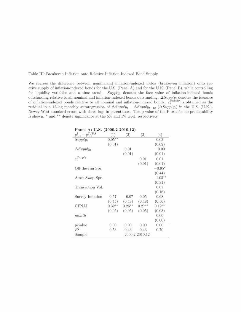
Table III: Breakeven Inflation onto Relative Inflation-Indexed Bond Supply.

We regress the difference between nominaland inflation-indexed yields (breakeven inflation) onto rel-ative supply of inflation-indexed bonds for the U.S. (Panel A) and for the U.K. (Panel B), while controllingfor liquidity variables and a time trend. Supplyt denotes the face value of inflation-indexed bondsoutstanding relative to all nominal and inflation-indexed bonds outstanding. ΔSupplyt denotes the issuanceof inflation-indexed bonds relative to all nominal and inflation-indexed bonds. εSupply

t is obtained as theresidual in a 12-lag monthly autoregression of ΔSupplyt − ΔSupplyt−12 (ΔSupplyt) in the U.S. (U.K.).Newey-West standard errors with three lags in parentheses. The p-value of the F-test for no predictabilityis shown. * and ** denote significance at the 5% and 1% level, respectively.

Panel A: U.S. (2000.2-2010.12)

y$n,t − yTIPSn,t (1) (2) (3) (4)

Supplyt 0.05∗∗ 0.03(0.01) (0.02)

ΔSupplyt 0.01 −0.00(0.01) (0.01)

εSupplyt 0.01 0.01

(0.01) (0.01)Off-the-run Spr. −0.95∗

(0.44)Asset-Swap-Spr. −1.05∗∗

(0.31)Transaction Vol. 0.07

(0.16)Survey Inflation 0.57 −0.07 0.05 0.68

(0.45) (0.49) (0.48) (0.56)CFNAI 0.32∗∗ 0.26∗∗ 0.27∗∗ 0.12∗∗

(0.05) (0.05) (0.05) (0.03)month 0.00

(0.00)p-value 0.00 0.00 0.00 0.00R2 0.53 0.43 0.43 0.70Sample 2000.2-2010.12

Table III (continued)

Panel B: U.K. (1986.1-2010.12 and 1999.11-2010.12)

y$n,t − yTIPSn,t (1) (2) (3) (4) (5)

Supplyt 0.07∗ 0.03 0.01(0.03) (0.03) (0.03)

ΔSupplyt 0.00 −0.00 −0.02(0.02) (0.05) (0.05)

εSupplyt 0.01 0.00 0.02

(0.02) (0.05) (0.05)Off-the-run Spr. −0.11

(0.11)LIBOR-GC Spr. 0.02

(0.03)Transaction Vol. −0.00∗∗

(0.00)Survey Inflation 0.11∗∗ 0.14∗∗ 0.14∗∗ 0.04∗∗ 0.06∗∗

(0.02) (0.01) (0.01) (0.02) (0.02)month 0.01∗∗ 0.01∗∗

(0.00) (0.00)p-value 0.00 0.00 0.00 0.00 0.00R2 0.54 0.51 0.51 0.87 0.88Sample 1986.1− 2010.12 1999.11− 2010.12

Table IV: Excess Bond Returns onto Relative Supply of Inflation-Indexed Bonds.

We regress overlapping 3-month nominal, inflation-indexed and breakeven log excess bond returnsonto measures of relative supply as defined in Table III while controlling for the nominal term spread, theTIPS term spread and the breakeven term spread and liquidity as estimated in Table II(4). Newey-Weststandard errors with three lags are provided in parentheses. The p-value of the F-test of no predictability isshown. * and ** denote significance at the 5% and 1% level, respectively.

Panel A: U.S. (2000.5-2010.12)(1) (2) (3) (4)

xr$n,t+1 xr$n,t+1 xrTIPSn,t+1 xrbn,t+1

Supplyt −0.21 −0.38 0.04 −0.42(0.73) (0.68) (0.71) (0.73)

ΔSupplyt 0.26 0.22 0.28 −0.06(0.55) (0.54) (0.41) (0.30)

εSupplyt −0.00 −0.00 −0.00 −0.00

(0.00) (0.00) (0.00) (0.00)Ln,t 1.64 7.03 18.02 −10.99

(9.87) (11.82) (10.20) (9.82)

y$n,t − y$1,t 2.11(1.41)

yTIPSn,t − yTIPS

1,t 0.77 2.53 −1.76(2.12) (1.39) (1.57)

bn,t − b1,t 4.18 −2.40 6.58∗

(3.18) (2.43) (2.68)p-value 0.39 0.44 0.01 0.03R2 0.05 0.05 0.21 0.20Sample 2000.5− 2010.12

Panel B: U.K. (1986.4-2010.12 and 2000.2-2010.12)(1) (2) (3) (4) (5) (6) (7) (8)

xr$n,t+1 xr$n,t+1 xrTIPSn,t+1 xrbn,t+1 xr$n,t+1 xr$n,t+1 xrTIPS

n,t+1 xrbn,t+1

Supplyt −1.26 −1.11 −0.24 −0.87 −1.42 −1.58 −1.90 0.33(1.09) (1.06) (0.78) (0.99) (1.67) (1.69) (1.69) (2.05)

ΔSupplyt −3.05 −3.70 −3.79 0.09 3.55 2.72 3.51 −0.79(5.78) (5.92) (3.23) (5.39) (5.39) (5.46) (3.73) (5.24)

εSupplyt 2.46 2.94 3.73 −0.79 −4.82 −4.10 −3.91 −0.19

(5.94) (6.04) (3.34) (5.53) (5.68) (5.68) (3.96) (5.67)Ln,t −10.77 −7.97 −13.26 5.29

(14.11) (14.61) (8.45) (11.21)

y$n,t − y$1,t 3.02∗ 2.05(1.52) (1.74)

yTIPSn,t − yTIPS

1,t 0.01 3.63∗ −3.62 0.02 2.76 −2.75(3.27) (1.75) (2.48) (2.82) (1.86) (2.15)

bn,t − b1,t 6.70 −2.30 9.00∗∗ 4.40 0.03 4.37(3.73) (2.00) (3.01) (4.38) (2.47) (2.62)

p-value 0.17 0.20 0.23 0.03 0.32 0.41 0.15 0.35R2 0.06 0.07 0.05 0.10 0.07 0.08 0.06 0.05Sample 1986.4− 2010.12 2000.2− 2010.12

Table V: Liquidity-Adjusted Bond Return Predictability.

We predict 3-month overlapping liquidity-adjusted excess log returns of inflation-indexed bonds andof nominal bonds in excess of inflation-indexed bonds using the liquidity-adjusted inflation-indexed termspread, the liquidity-adjusted breakeven term spread, and the liquidity differential Ln,t. Ln,t is estimatedas the negative of the variation explained by liquidity variables in Table II(4). rLn,t+1 is the return oninflation-indexed bonds due to illiquidity. Newey-West standard errors with three lags in parentheses.The p-value of the F-test for no predictability is shown. We show one-sided bootstrap p-values from 2000replications to account for the fact that liquidity is estimated. We use block bootstrap with block length 24months.

Panel A: U.S. (1999.6-2010.12)(1) (2) (3) (4) (5) (6)

xrTIPS−Ln,t+1 xrTIPS−L

n,t+1 xrb+Ln,t+1 xrb+L

n,t+1 rLn,t+1 rLn,t+1(yTIPSn,t − Ln,t

)− yTIPS1,t 3.04 2.31 −1.31 0.24

Newey-West SE (1.35) (1.81) (1.53) (0.66)Bootstrap p-value 15.3% 23.9% 33.8% 44.5%

(bn,t + Ln,t)− b1,t −0.22 4.55 5.20 −0.87Newey-West SE (2.91) (1.75) (1.75) (1.74)

Bootstrap p-value 17.9% 0.1% 0.0% 32.5%Ln,t 6.88 −6.76 11.49 11.03

Newey-West SE (10.14) (7.50) (2.92) (3.53)Bootstrap p-value 23.0% 15.5% 0.1% 0.1%

Const. −0.00 −0.01 −0.01 0.01 −0.02 −0.02Newey-West SE (0.01) (0.02) (0.00 (0.01) (0.01) (0.01)

Bootstrap p-value 68.7% 10.0% 14.6% 6.4% 11.6% 15.9%p-value 0.03 0.16 0.01 0.02 0.00 0.00R2 0.06 0.07 0.08 0.13 0.17 0.17Sample 1999.6− 2010.12

Panel B: U.K. (2000.2-2010.12)(1) (2) (3) (4) (5) (6)

xrTIPS−Ln,t+1 xrTIPS−L

n,t+1 xrb+Ln,t+1 xrb+L

n,t+1 rLn,t+1 rLn,t+1(yTIPSn,t − Ln,t

)− yTIPS1,t 4.99 5.52 −4.76 −2.44

Newey-West SE (2.13) (2.71) (3.16) (1.75)Bootstrap p-value 4.1% 4.2% 4.2% 9.0%

(bn,t + Ln,t)− b1,t −4.28 4.59 8.38 4.14Newey-West SE (3.10) (3.77) (4.20) (2.42)

Bootstrap p-value 24.0% 0.7% 0.8% 17.6%Ln,t −20.42 14.16 18.67 17.93

Newey-West SE (12.02) (14.17) (7.15) (7.24)Bootstrap p-value 8.3% 15.7% 0.0% 0.0%

Const. 0.00 0.04 −0.01 −0.04 −0.02 −0.03Newey-West SE (0.01) (0.02) (0.01) (0.02) (0.01) (0.01)

Bootstrap p-value 31.7% 5.7% 1.8% 5.2% 2.3% 2.1%p-value 0.02 0.00 0.23 0.01 0.01 0.00R2 0.06 0.13 0.03 0.12 0.13 0.19Sample 2000.2− 2010.12

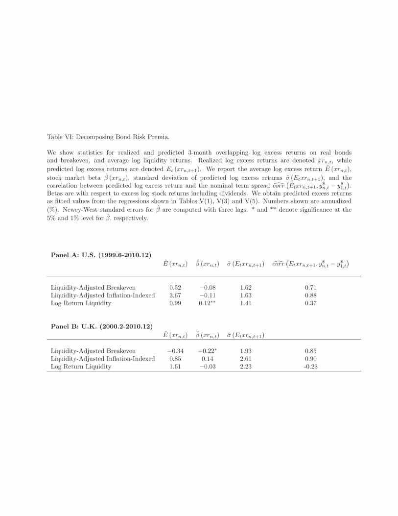
Table VI: Decomposing Bond Risk Premia.

We show statistics for realized and predicted 3-month overlapping log excess returns on real bondsand breakeven, and average log liquidity returns. Realized log excess returns are denoted xrn,t, while

predicted log excess returns are denoted Et (xrn,t+1). We report the average log excess return E (xrn,t),

stock market beta β (xrn,t), standard deviation of predicted log excess returns σ (Etxrn,t+1), and thecorrelation between predicted log excess return and the nominal term spread corr

(Etxrn,t+1, y

$n,t − y$1,t

).

Betas are with respect to excess log stock returns including dividends. We obtain predicted excess returnsas fitted values from the regressions shown in Tables V(1), V(3) and V(5). Numbers shown are annualized

(%). Newey-West standard errors for β are computed with three lags. * and ** denote significance at the

5% and 1% level for β, respectively.

Panel A: U.S. (1999.6-2010.12)

E (xrn,t) β (xrn,t) σ (Etxrn,t+1) corr(Etxrn,t+1, y

$n,t − y$1,t

)

Liquidity-Adjusted Breakeven 0.52 −0.08 1.62 0.71Liquidity-Adjusted Inflation-Indexed 3.67 −0.11 1.63 0.88Log Return Liquidity 0.99 0.12∗∗ 1.41 0.37

Panel B: U.K. (2000.2-2010.12)

E (xrn,t) β (xrn,t) σ (Etxrn,t+1)

Liquidity-Adjusted Breakeven −0.34 −0.22∗ 1.93 0.85Liquidity-Adjusted Inflation-Indexed 0.85 0.14 2.61 0.90Log Return Liquidity 1.61 −0.03 2.23 -0.23

Panel A: U.S. (1999.3-2010.12)

-1.5

-1-.

50

Tra

nsac

tion

Vol

.

0.5

11.

5A

nnua

lized

(%

)

99 00 01 02 03 04 05 06 07 08 09 10Year

Off-the-Run Spread Asset-Swap SpreadSynthetic Minus Cash Transaction Vol. (Right)

Panel B: U.K. (1999.11-2010.12)

-1.5

-1-.

50

Tra

nsac

tion

Vol

.

0.5

11.

52

2.5

Ann

ualiz

ed (

%)

99 00 01 02 03 04 05 06 07 08 09 10Year

Off-the-Run Spread LIBOR-GC SpreadTransaction Vol. (Right)

Figure 1: U.S. and U.K. Liquidity Proxies.

We use liquidity proxies to estimate differential liquidity between inflation-indexedand nominal government bonds. For the U.S., we use the spread between off-the-run andon-the-run 10 year nominal bond yields, the relative inflation-indexed bond log transactionvolume, the asset-swap differential, and the difference between synthetic and cash breakeven.For the U.K., we use the difference between a 10 year nominal fitted par yield and the 10year nominal generic Bloomberg yield, denoted “off the run”. We normalize the maximaof relative transaction volumes to zero. The asset-swap spread differential, synthetic minuscash breakeven, and the GBP three-month LIBOR-GC spread proxy for the cost of fundinga levered investment in inflation-indexed bonds.

Panel A: U.S. (1999.3-2010.12)

-.5

0.5

11.

52

Ann

ualiz

ed (

%)

99 00 01 02 03 04 05 06 07 08 09 10Year

Panel B: U.K. (1999.11-2010.12)

-.5

0.5

11.

52

Ann

ualiz

ed (

%)

99 00 01 02 03 04 05 06 07 08 09 10year

Figure 2: Estimated U.S. and U.K. Liquidity Premia.

We estimate liquidity premia as the negative of the variation in breakeven explainedby liquidity proxies. Formally, Ln,t = −a2Xt, where Xt is the vector of liquidity variablesand a2 is the vector of corresponding estimated coefficients in Table II(4), Panels A and B.

Panel A: U.S. (1999.3-2010.12)

0.5

11.

52

2.5

33.

54

4.5

Ann

ualiz

ed (

%)

99 00 01 02 03 04 05 06 07 08 09 10Year

U.S. Breakeven Liquidity-Adjusted U.S. Breakeven

Panel B: U.K. (1999.11-2010.12)

0.5

11.

52

2.5

33.

54

4.5

Ann

ualiz

ed (

%)

99 00 01 02 03 04 05 06 07 08 09 10Year

U.K. Breakeven Liquidity-Adjusted U.K. Breakeven

Figure 3: Liquidity-Adjusted U.S. 10 Year Breakeven and U.K. 20 Year Breakeven.

Liquidity-adjusted breakeven equals breakeven plus the liquidity premium shown inFigure 2.

Panel A: U.S. (2000.2-2010.12)

05

1015

(%)

.51

1.5

22.

53

Ann

ualiz

ed (

%)

99 00 01 02 03 04 05 06 07 08 09 10Year

U.S. Breakeven Relative Supply U.S. TIPS (Right)

Panel B: U.K. (1986.1-2010.12)

1015

20(%

)

23

45

6A

nnua

lized

(%

)

85 90 95 00 05 10year

Breakeven Relative Supply Linkers (Right)

Figure 4: Relative Supply of Inflation-Indexed Bonds and Breakeven.

Relative supply shows the face value of inflation-indexed bonds outstanding relativeto the face value of inflation-indexed and nominal bonds outstanding. We show 10 yearU.S. breakeven and 20 year U.K. breakeven.

Panel A: U.S. (1999.6-2010.12)

-50

510

15A

nnua

lized

(%

)

99 00 01 02 03 04 05 06 07 08 09 10Year

U.S. Liquidity RP U.S. Real Rate RPU.S. Inflation RP

Panel B: U.K. (2000.2-2010.12)

-10

-50

510

15A

nnua

lized

(%

)

99 00 01 02 03 04 05 06 07 08 09 10Year

U.K. Liquidity RP U.K. Real Rate RPU.K. Inflation RP

Figure 5: U.S. and U.K. Estimated Risk Premia.

Predicted 3-month excess returns in annualized units, labeled real rate risk premia,inflation risk premia, and liquidity risk premia. We obtain predicted excess returns as fittedvalues from the regressions shown in Tables V(1), V(3) and V(5), Panels A and B.