Restoring Ramsey tax lessons to Mirrleesian tax settings:Atkinson-Stiglitz and Ramsey reconciled∗

Helmuth CremerToulouse School of Economics

(University of Toulouse and Institut universitaire de France)Toulouse, France

Firouz GahvariDepartment of Economics

University of Illinois at Urbana-ChampaignUrbana, IL 61801, USA

May 2012, revised February 2016

∗This paper has been presented in seminars at CESifo, Uppsala University, the Universityof Cologne and University Nova (Lisbon). We thank all the participants and in particular FelixBiebrauer, Sören Blomquist, Denis Epple, Kenneth Kletzer, Etienne Lehmann and CatarinaReis for their helpful suggestions and comments. We also thank Jean-Tirole for a number ofinspiring discussions about the underlying problem.

Abstract

This paper restores many of the Ramsey tax/pricing lessons considered as outdatedby the optimal tax approach to the Atkinson and Stiglitz (1976) framework whereindifferential commodity taxes are considered to be redundant. The key to this finding isincorporating a “break-even”constraint for public firms into the Atkinson and Stiglitzframework. Break-even constraints are fundamental to the regulatory pricing literaturebut have somehow been overlooked in the optimal tax literature. This reconciles theoptimal-tax and the regulatory-pricing views on Ramsey tax/pricing rules.

JEL classification: H2, H5.

Keywords: Ramsey taxes and pricing, break-even constraints, optimal tax literature,Atkinson and Stiglitz framework, regulatory pricing literature.

1 Introduction

In a recent contribution, Stiglitz (2015) discusses the importance of Frank Ramsey’s

1927 classic paper on optimal taxation; referring to it as “brilliant”and a paper that

“can be thought of as launching the field of optimal taxation and revolutionising public

finance” (p. 1). Nevertheless, Stiglitz goes on to conclude his paper’s Introduction

by this observation “... later analyses showed crucial qualifications, so that the policy

relevance of Ramsey’s analysis may be limited”. This paper calls for a reexamination

of these “qualifications”. They, we shall argue, stem from a Mirrleesian approach to

optimal taxation that ignores public firms’ break-even constraints. Yet, in practice,

regulation is almost always associated with budget balancing requirement. A fact that

has not escaped the attention of regulatory pricing literature forming a cornerstone of

regulatory economics.1

Prior to Mirrlees (1971), the Ramsey tax framework served as a cornerstone of the

optimal tax theory. The central question in this literature was that of designing (linear)

commodity taxes to collect a given tax revenue. Labor income went generally untaxed

or subjected to a linear tax. The main point made in this literature was that, except in

very special cases, commodity taxes should not be uniform and that they should be set to

balance effi ciency and equity considerations. The effi ciency aspects manifest themselves

most clearly in the inverse-elasticity rules (derived when demand functions, Hicksian

or Marshallian are separable). These effi ciency-driven tax rules entail a regressive bias

in that goods with low price-elasticities are often necessities consumed proportionately

more by poorer households. This bias is then mitigated by the equity terms in the tax

rules (often appearing as covariance terms). These tend to increase the tax rate on

1 It is a mystery as to why it took the public finance literature more than four decades and untilearly 1970s to appreciate Ramsey’s (1927) insights. It started with the seminal paper by Diamond andMirrlees (1971) and followed by literally hundreds of papers. Baumol and Bradford (1970) and Sandmo(1976) provide an interesting history of this subject. In the original Ramsey problem, individuals arealike and there is no income tax. With heterogeneous individuals, one also allows for a uniform lump-sumtax or rebate (and possibly a linear tax on labor income); see Diamond (1975).

1

goods that are consumed proportionately more by richer households.

The Mirrleesian approach posed a serious challenge to the Ramsey tax framework

approach and the lessons drawn from it. Mirrlees (1971) argued that the existence

or absence of tax instruments must be rationalized on the basis of the informational

constraints in the economy. This approach turns the Ramsey tax framework on its head

by making nonlinear income taxation the most powerful tax instrument at the disposal

of the government. In turn, the reliance on the nonlinear income tax has a devastating

implication for the usefulness of commodity taxes. In their classic contribution, Atkinson

and Stiglitz (1976) show that under some conditions– weak separability of preferences

in labor supply and goods– an optimal nonlinear income tax is suffi cient to implement

any incentive compatible Pareto-effi cient allocation. In other words, commodity taxes

are redundant (or should be uniform). The Ramsey results come about, it is thus

argued, merely as an artifact of restricting the income tax to be linear (an ad hoc and

inconsistent assumption given the assumed informational structure). The Atkinson and

Stiglitz (AS) result has had a tremendous effect in shaping the views of public economists

concerning the design of optimal tax systems: In particular that prices should not be

used for redistribution (even in a second best setting), and that in-kind transfers are

not useful.2

A prominent public economics specialist summarizes his and the prevailing view in

the literature this way: “Once we add the nonlinear income tax, if we keep homogeneous

preferences and weak separability of labor, we have the following generalized view:

The equity-effi ciency tradeoff associated with income taxation is addressed with the

2 It is by now well understood though that the AS result also has its own limitations. In particular,it may not hold under uncertainty (Cremer and Gahvari, 1995) or under multi-dimensional heterogene-ity (Cremer, Gahvari and Ladoux, 1998, and Cremer, Pestieau and Rochet, 2001) and redistributionthrough prices may then once again be second-best optimal (Cremer and Gahvari, 1998 and 2002). Still,these limitations notwithstanding, it is fair to say that the Ramsey approach to taxation is consideredas dated and no longer “state of the art”. It does continue to occupy a prominent place in all advancedtextbooks, but it is taught mainly as an introduction to tax design and not because of its practicalrelevance.

2

income tax (as done by Mirrlees), and we should follow Economics 101 first-best rules

in other realms: uniform commodity taxes (so as not to distort consumption), public

goods according to the Samuelson rule, marginal cost pricing, and so forth” (private

correspondence).

This strong view notwithstanding, the Ramsey-type rules have had a more or less

independent second– or some might argue first– life as a model of regulatory pricing.3

In his pioneering paper that appeared prior to Mirrlees (1971), Boiteux (1956) studied

linear pricing of a regulated multi-product monopoly that has to cover some “fixed cost”

(for instance the infrastructure cost of the network). This is to be achieved through

markups on the monopoly’s different products (equivalent to taxes).4 Formally, this

problem is equivalent to a Ramsey tax model with the fixed cost playing the role of the

government’s tax revenue requirement.

To sum, optimal tax and regulatory pricing literatures appear to have diverged in the

way they view the practical relevance of the AS result (see Section 2.1 below). Whereas

Ramsey pricing is considered totally passé in the optimal tax literature (even by Econ

101 standard according to our earlier quote from a prominent expert), Ramsey-type

lessons permeate the field of regulatory economics. This is quite surprising considering

the fact that the issues the two literatures address have an identical formal structure.

In both cases, there is a public authority whose objective is to raise a fixed amount of

revenue (where the revenue finances the government’s expenditures in the optimal tax

literature and the firms’fixed costs in the regulation literature).5 This paper is thus

also an attempt to reconcile these divergent views and bring them together. To this

3While it is true that regulators and especially competition authorities are often reluctant to acceptRamsey pricing arguments, this is not because of the AS result. Their objection is more of legal andprocedural nature. In particular, Ramsey prices are often viewed as “discriminatory” and subject toinformational problems when the operator is better informed about demand condition than the regulator.

4We follow the terminology used in the regulation literature but, in reality, this is a quasi-fixed costrelevant also in the long-run (a non convexity in the production set).

5Redistributive concerns are not confined to the tax literature and also appear in the regulatoryeconomics literature.

3

end, we incorporate the regulatory economics focus on budget balance into a Mirrleesian

optimal tax framework. As far as we know, a comprehensive analysis of this sort has

not been attempted before.

The optimal tax setting we consider combines nonlinear income taxation with linear

taxation/pricing of consumption goods. The informational structure that underlies this

setting is now standard in the Mirrleesian optimal taxation literature. First, individ-

uals’earning abilities and labor supplies are not publicly observable, but their pre-tax

incomes are. This rules out type-specific lump-sum taxes but allows for nonlinear in-

come taxation. Second, individual consumption levels of goods, whether subject to

regulation or not, are not observable so that nonlinear taxation and/or pricing of goods

are not possible. On the other hand, anonymous transactions are observable making

linear commodity taxation feasible.

To account for the regulatory economics balanced budget concerns, we assume that

a subset of the goods are produced by a public or regulated firm that has to cover a

fixed cost through markups on the different commodities it sells.6 This latter constraint

gives rise to a “break-even”constraint on the part of the firm. This comes on top of the

overall government’s budget constraint. In other words, while our setting is that of AS,

we depart from the existing optimal tax literature by formally incorporating a binding

break-even in our model. Break-even constraints are fundamental to the regulatory

pricing literature; yet somehow they have been overlooked in the optimal tax literature.

We draw on this literature to show that there exist good justifications for imposing

such a constraint. Some are due to informational issues pertaining to the opportunity

to invest in a given sector or the incentives to reduce costs.7

While we optimize over all tax instruments including income, we are not concerned

6Whether this firm is public, as in Boiteux’s world, or private but regulated does not matter. Eitherway, one implicitly assumes that the firms’revenues must also cover some “fair”rate of return on capital.

7We will not formally model these type of informational asymmetries in this paper. However, weshall return to this issue in the Conclusion and provide some indication on how our results would beaffected if this extra source of information asymmetry were considered.

4

with the properties of the income tax schedule. Our aim is to solely study the commodity

taxation and pricing rules (for goods produced by public/regulated firms as well as

those produced subject to no regulation). We derive these rules for general preferences

but concentrate on the case of weakly-separable preferences between labor supply and

goods that underlies the AS result. We shall refer to this environment as the AS

setting/framework/model and contrast it with the Ramsey environment wherein all

tax instruments are linear. The fundamental contribution of our paper is that the AS

setting with a break-even constraint restores many of the traditional Ramsey tax/pricing

features that have been questioned by modern optimal tax theory.

Specifically, we demonstrate that, given a break-even constraint, not only is it de-

sirable to tax the goods produced by the public/regulated firm but also other goods.

Intuitively, taxation of privately-produced goods are generally needed to offset the dis-

tortions created by the public/regulated firm’s departure from marginal cost pricing.

This result stands in sharp contrast to AS result on the redundancy of commodity taxes.

We then illustrate and elaborate on our findings by studying a simple framework with

one publicly-provided and two privately-provided goods.

To interpret our results, and for comparison purposes, we also recast and derive the

pricing rules for a setting wherein nonlinear income taxation is ruled out, and taxes

and markups are used to finance both a revenue requirement and a fixed cost (rather

than only one of the two as is traditionally done in Ramsey models). While this yields

predictable results and is not of much interest in itself, it is a useful reference point.

It encapsulates the effects of imposing a break-even constraint in a Ramsey setting

and thus serves as a benchmark for understanding and interpreting our results (derived

for the AS setting with a break-even constraint). We present this benchmark as an

Appendix to the paper. Comparing the results derived in our setting to those in this

benchmark highlights and isolates the role that commodity taxes do play in the AS

setting (contrary to the AS’s own “no role”result).

5

The two special cases of independent Hicksian and independent Marshallian demand

curves provide further insights into the nature of the tax/pricing rules in our model.

In the separable Hicksian demand case, we find that private goods (not included in

the break-even constraint) should go untaxed. On the other hand, public firms should

follow pricing rules that are purely effi ciency-driven and Ramsey type: Goods are taxed

inversely to their compensated demand elasticity regardless of their distributional impli-

cations. Redistribution is taken care of by the income tax (allowing public firms’prices

to be adjusted for revenue raising as in the Ramsey model with identical individuals).

This is to be contrasted with today’s prevailing view– based on the AS framework that

ignores break-even constraints– that commodity taxes are redundant. It also differs

from earlier Ramsey pricing views that commodity taxes should follow inverse elasticity

rules adjusted for redistributive concerns.

Results become less predictable in the case where Marshallian demands are inde-

pendent. Here, allowing for a break-even constraint in the AS framework, resurrects a

role for commodity taxes that go beyond the goods produced subject to the break-even

constraint. Instead, it spills over to the taxation of other goods as well. One con-

tinues to get inverse elasticity rules as in the Ramsey model; however, their structure

differs from the traditional expressions in the Ramsey model. On the one hand, they

are more complicated than the pure effi ciency rules. On the other hand, there is no

covariance (or similar) term that captures redistributive considerations. Instead, they

contain “tax revenue terms” that measure the social value of the extra tax revenues

generated from demand variations that follow the (compensating) adjustments in dis-

posable income. These terms lead to predictions that are similar to those coming from

the many-household Ramsey model albeit without redistributive concerns; namely, that

goods with higher demand elasticities should be taxed more heavily.

Finally, we study what is arguably the most celebrated general result obtained in

the Ramsey model; namely, the (un)equal proportional reduction in compensated de-

6

mands property. We show that, in contrast to the single-household Ramsey model, the

reductions differ across goods. This in and of itself is not particularly surprising given

the presence of heterogeneous households. More interestingly, compared to the many-

household Ramsey model with the break-even constraint, we find that the redistributive

considerations are once again replaced by tax revenue terms.

2 The model

There are H types of individuals, indexed j = 1, 2 . . . , H, who differ in their wages,

wj , but have identical preferences over goods and leisure.8 All goods are produced at

a constant marginal cost which we normalize to one. Some, x = (x1, x2, . . . , xn), are

produced by the private sector; the rest, y = (y1, y2, . . . , ym) are produced by a public

or regulated firm which incurs a fixed cost. The firm is constrained to break even by

marking up its marginal costs.9 Let p = (p1, p2, . . . , pn) denote the consumer price

of x and q = (q1, q2, . . . , qn) the consumer price of y. Finally, denote the commodity

tax rates on x by t = (t1, t2, . . . , tn) and the public firms’commodity-tax-cum-mark-

ups by τ = (τ1, τ2, . . . , τm). We have pi = 1 + ti (i = 1, 2, . . . , n) and qs = 1 + τ s

(s = 1, 2, . . . ,m).

Individual consumption levels are not publicly observable but anonymous transac-

tions can be observed. Consequently, commodity taxes must be proportional and public

sector prices are linear. For the remaining variables, the information structure is the

one typically considered in mixed taxation models; see e.g., Christiansen (1984) and

Cremer and Gahvari (1997). In particular, an individual’s type, wj , and labor input,

Lj , are not publicly observable; his before-tax income, Ij = wjLj , on the other hand,

is. Consequently, type-specific lump-sum taxation is ruled out but non-linear taxation

of incomes is feasible.8Our results will not change if a continuous distribution of types are considered.9Alternatively one can think of a privately owned regulated firm whose prices are set to cover cost

plus a fair rate of return on capital.

7

To characterize the (constrained) Pareto-effi cient allocations we derive an optimal

revelation mechanism. For our purpose, a mechanism consists of a set of type-specific

before-tax incomes, Ijs, aggregate expenditures on private sector and public sector

goods, cjs, and two vectors of consumer prices (same for everyone) p and q (for x

and y). To proceed further, it is necessary to consider the optimization problem of an

individual for a given mechanism (p, q, c, I). Formally, given any vector (p, q, c, I), an

individual of type j maximizes utility u = u(x, y, I/wj

)subject to the budget constraint∑n

i=1 pixi +∑m

s=1 qsys = c. The resulting conditional demand functions for x and y are

denoted by xi = xi(p, q, c, I/wj

)and ys = ys

(p, q, c, I/wj

).10 Substituting in the utility

function yields the conditional indirect utility function

v(p, q, c, I/wj

)≡ u

[x(p, q, c, I/wj

), y(p, q, c, I/wj

), I/wj

].

Thus, a j-type individual who is assigned cj , Ij will have demand functions and an

indirect utility function given by

xji = xi(p, q, cj , Ij/wj), (1)

yjs = ys(p, q, cj , Ij/wj

), (2)

vj = v(p, q, cj , Ij/wj

). (3)

Similarly, the demand functions and the indirect utility function for a j-type who claims

to be of type k, the so-called mimicker, is given by

xjki = xi(p, q, ck, Ik/wj), (4)

yjks = ys

(p, q, ck, Ik/wj

), (5)

vjk = v(p, q, ck, Ik/wj

). (6)

10These demand functions are derived conditional on a given I. Hence the conditional qualifier.

8

2.1 The break-even constraint

The information structure posited above describes only the informational asymmetries

between the tax administration and the taxpayers typically assumed in the optimal

tax literature. This does not rationalize a break-even constraint which is the missing

link between the optimal tax and regulatory economics literatures. In settings where

tax policy is restricted only by informational considerations of this type, break-even

constraints could be undone by simple lump-sum transfers from the government to the

operators. Yet, in practice, regulation is almost always associated with budget balancing

requirements. Which explains why they form a cornerstone of regulatory economics.

2.1.1 Break-even constraints in regulatory economics

Ramsey-Boiteux (RB) pricing continues to play an important role in the sectors still

subject to some form of regulation even though, over the last few decades, the scope

of regulation has declined. A prominent example is the postal sector in the US where

Ramsey-Boiteux pricing remains an important benchmark in regulatory hearings; see

Crew and Kleindorfer (2011, 2012). As a matter of fact, not only has RB pricing kept its

position but it has even found new applications in setting of regulatory reform and mar-

ket liberalization. For instance, while the original Boiteux model concerns a monopoly,

Ware and Winter (1985) show that generalized RB rules prevail in imperfectly compet-

itive markets. Furthermore, Laffont and Tirole (1990) argue that one should price the

network access an incumbent operator has to provide to its upstream competitors on

the basis of RB logic.

Another interesting result, shown by Vogelsang and Finsinger (1979), is that Ramsey

prices can be decentralized through an iterative procedure based on a global price cap;

see also Laffont and Tirole (2000, page 67). More generally, in the literature on incentive

regulation, Ramsey prices are viewed as a kind of “ideal” solution: they represent a

so-called “full information” benchmark. One should bear in mind, however, that the

9

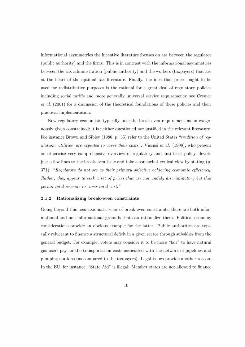
informational asymmetries the incentive literature focuses on are between the regulator

(public authority) and the firms. This is in contrast with the informational asymmetries

between the tax administration (public authority) and the workers (taxpayers) that are

at the heart of the optimal tax literature. Finally, the idea that prices ought to be

used for redistributive purposes is the rational for a great deal of regulatory policies

including social tariffs and more generally universal service requirements; see Cremer

et al. (2001) for a discussion of the theoretical foundations of these policies and their

practical implementation.

Now regulatory economists typically take the break-even requirement as an exoge-

nously given constrained; it is neither questioned nor justified in the relevant literature.

For instance Brown and Sibley (1986, p. 35) refer to the United States “tradition of reg-

ulation: utilities’are expected to cover their costs”. Viscusi et al. (1998), who present

an otherwise very comprehensive overview of regulatory and anti-trust policy, devote

just a few lines to the break-even issue and take a somewhat cynical view by stating (p.

371): “Regulators do not see as their primary objective achieving economic effi ciency.

Rather, they appear to seek a set of prices that are not unduly discriminatory but that

permit total revenue to cover total cost.”

2.1.2 Rationalizing break-even constraints

Going beyond this near axiomatic view of break-even constraints, there are both infor-

mational and non-informational grounds that can rationalize them. Political economy

considerations provide an obvious example for the latter. Public authorities are typi-

cally reluctant to finance a structural deficit in a given sector through subsidies from the

general budget. For example, voters may consider it to be more “fair”to have natural

gas users pay for the transportation costs associated with the network of pipelines and

pumping stations (as compared to the taxpayers). Legal issues provide another reason.

In the EU, for instance, “State Aid”is illegal: Member states are not allowed to finance

10

their operators’deficits through subsidies.11

The information-based rationalizations are not explicitly addressed in our setting.

These are summarized by Laffont and Tirole (1993, pp 23—30). They give two basic

arguments. One, which they ascribe to Coase (1945, 1946), applies to “a firm or a

product whose existence is not a forgone conclusion”. Unless an activity at least breaks

even, one cannot be sure that its production is beneficial for the society to warrant

the government covering its fixed costs. Roughly speaking, Coase argues that, absent a

budget constraint, the government is entrusted to make this decision without having the

appropriate information. With a break-even constraint, this decision is effectively made

by consumers who thereby reveal if their willingness to pay for the product is suffi ciently

high. The second argument is related to incentives associated with informational asym-

metries between the regulator and the firm (which we do not formally model).12 For

instance, Allais (1947) has argued that the absence of a break-even constraint would

create “inappropriate incentives for cost reduction”.

2.2 Constrained Pareto-effi cient allocations

Denote the government’s external revenue requirement by R and the fixed costs of

public firms by F. Constrained Pareto-effi cient allocations are described, indirectly, as

follows.13 MaximizeH∑j=1

ηjv(p, q, cj , Ij/wj

)(7)

11Unless the aid comes as a compensation for specific public-service obligations imposed on an op-erator. The State Aid legislation is in turn motivated by anti-trust considerations and specifically theconcern that member states might subsidize their “national champion”.12We discuss this issue further in the Conclusion.13 Indirectly because the optimization is over a mix of quantities and prices. Then, given the com-

modity prices, utility maximizing individuals would choose the quantities themselves.

11

with respect to p, q, cj and Ij where ηjs are constants with the normalization∑H

j=1 ηj =

1.14 The maximization is subject to the resource constraint

H∑j=1

πj

[(Ij − cj) +

n∑i=1

(pi − 1)xji +

m∑s=1

(qs − 1)yjs

]≥ R+ F, (8)

the break-even constraint

H∑j=1

πj

[m∑s=1

(qs − 1)yjs

]≥ F, (9)

and the self-selection constraints

vj ≥ vjk, j, k = 1, 2, . . . ,H. (10)

Denote the Lagrangian expression by L, and the Lagrangian multipliers associated

with the resource constraint (8) by µ, the public firms’break-even constraint (9) by δ,

and with the self-selection constraints (10) by λjk. We have

L =∑j

ηjvj + µ

∑j

πj

[(Ij − cj) +

n∑i=1

(pi − 1)xji +

m∑s=1

(qs − 1)yjs

]− R− F

+δ

∑j

πj

[m∑s=1

(qs − 1)yjs

]− F

+∑j

∑k 6=j

λjk(vj − vjk). (11)

The first-order conditions of this problem with respect to Ij , cj , for j, k = 1, 2, . . . ,H,

and pi, qs, for i = 2, 3, . . . , n, and s = 1, 2, . . . ,m, characterize the Pareto-effi cient

allocations constrained both by the public firms’break-even constraint, the resource

constraint, the self-selection constraints, as well as the linearity of commodity tax rates

(see the paragraph below as to why the optimization does not extend to i = 1). They

are derived in Appendix A.15

14The maximization must leave one of the prices out; see the discussion at the end of this Section.15We assume that the second-order conditions are satisfied. Their violation is only interesting in

conjunction with the properties of the income tax schedule and the question of bunching.

12

The reason that we do not optimize over p1 is well-known in the optimal tax liter-

ature. With x and y being homogeneous of degree zero in p, q, and c, consumer prices

can determined only up to a proportionality factor. Consequently, one of the consumer

prices must be normalized. We choose p1 and set its value at p1 = 1.16 Having stated

this, a caveat is in order. In the absence of the break-even constraint, the normalization

of one of the consumer prices is without any loss of generality. In our setting, the fact

that consumer prices can be determined only up to a proportionality factor implies, at

first glance, that the break-even constraint may be rendered inconsequential. This is the

idea that the government can always raise all prices proportionately to cover the break-

even constraint of the public firm! However, imposing a binding break-even constraint

also rules out the possibility of an across the board uniform increase in all consumer

prices, including those of the public firm, for the revenues of the public firm to cover its

fixed costs. Indeed, such an across the board increases in all prices is in contradiction

with the very idea of imposing a break-even constraint in the first place. This “policy”

will never work when there are multiple firms with different cost structures.17

3 Atkinson and Stiglitz theorem and optimal commoditytaxes

In the standard mixed taxation model without the break-even constraint, assuming

preferences are weakly separable in goods and labor supply, the Atkinson and Stiglitz

(1976) theorem on the redundancy of commodity taxes holds. The particular feature of

separability that drives the AS result is the property that a j-type who pretends to be

16Observe that with p1 = 1, one can replace∑n

i=1(pi − 1)xji in (11) with∑n

i=2(pi − 1)xji .17Suppose there are two public firms. Refer to the one which has a relatively higher fixed cost as #1

and the other as #2. Raising prices proportionately to balance the budget of #1 must imply that #2will have a surplus, while raising them to balance the budget of #2 must imply that #1 will have adeficit.

13

of type k will have the same demand as type k. That is,

xjki = xki = xi(p, q, ck), (12)

yjks = yks = ys

(p, q, ck

). (13)

This arises because with weak-separability, preferences take the following form u =

u(f(x, y), I/wj

). Under this circumstance, the (conditional) demand functions for x

and y specified in equations (1)—(2) and (4)—(5) will be independent of I/wj so that

xi = xi(p, q, c

)and ys = ys

(p, q, c

). Moreover, the indirect utility function too will be

weakly separable in(p, q, c

)and I/wj and written as v

(φ(p, q, c

), I/wj

).

The above property has far reaching implications for optimal commodity taxes in

our setting too; both those produced by the public firm as well as privately. To derive

these, introduce the compensated version of demand functions (1)—(2). Specifically,

denote the compensated demand for a good by a “tilde”over the corresponding variable.

Let ∆ denote the (n+m− 1) × (n+m− 1) matrix derived from the Slutsky matrix,

aggregated over all individuals, by deleting its first row and column,

∆ =

∑j π

j ∂xj2

∂p2· · ·

∑j π

j ∂xj2

∂pn

∑j π

j ∂xj2

∂q1· · ·

∑j π

j ∂xj2

∂qm...

. . ....

.... . .

...∑j π

j ∂xjn

∂p2· · ·

∑j π

j ∂xjn

∂pn

∑j π

j ∂xjn

∂q1· · ·

∑j π

j ∂xjn

∂qm∑j π

j ∂yj1

∂p2· · ·

∑j π

j ∂yj1

∂pn

∑j π

j ∂yj1

∂q1· · ·

∑j π

j ∂yj1

∂qm...

. . ....

.... . .

...∑j π

j ∂yjm

∂p2· · ·

∑j π

j ∂yjm

∂pn

∑j π

j ∂yjm

∂q1· · ·

∑j π

j ∂yjm

∂qm

. (14)

We prove in Appendix A that in this case optimal commodity taxes satisfy the following

14

equations,18

t2...tn(

1 + δµ

)τ1

...(1 + δ

µ

)τm

= − δ

µ∆−1

0...0∑j π

jyj1...∑

j πjyjm

. (15)

The implication of equation (15) stands in sharp contrast to the prevailing view in

the literature as summarized in the quote we gave in the Introduction. It demonstrates

quite clearly that, notwithstanding the Atkinson and Stiglitz (1976) theorem, t = 0

and τ = 0 are not a solution to (15). Commodity taxes and departures from marginal

cost pricing are necessary components of Pareto-effi cient tax structures. The so-called

“Economics 101”intuition appears to be a false one!

Equally crucial is to realize that the underlying reason for this result is the existence

of the “break-even” constraint. To see this, observe that if F = 0, i.e. if there is no

fixed cost, the break-even constraint becomes irrelevant and thus non-binding in our

optimization problem. Under this circumstance, δ = 0 and the right-hand side of (15)

is reduced to a vector of n+m− 1 zeros. One then obtains ti = 0 and τ s = 0 (marginal

cost pricing) for all i = 1, 2, . . . , n and s = 1, 2, . . . ,m, and returns to the Atkinson

and Stiglitz result that commodity taxes are redundant. With F > 0, the break-even

constraint is necessarily violated under marginal cost pricing so that δ > 0. In this

case, the first n elements of the vector in the right-hand side of (15) continue to be zero,

but the other m elements differ from zero. It then follows that the solution no longer

implies all ts and all τs are zero. Nor will it be the case that the ts are necessarily zero.

This point, that the existence of a break-even point requires not only the taxation of

goods produced by the public firm but also the taxation of privately-provided goods,

constitutes the major lesson of our study.

18Observe that ∆ is of full rank so that its inverse exists; see Takayama (1985).

15

The second important lesson we are seeking to answer is the extent to which the pric-

ing rules defined by (15) resemble the traditional Ramsey rules. Traditionally, however,

the Ramsey pricing rules are derived for either a unified government budget constraint

(in the public finance literature), or for a public firm (in the regulation literature), but

not for the two together as we have done here. Adding on a break-even constraint to

the government’s budget constraint in the Ramsey problem, however, does not change

the structure of Ramsey taxes/pricing rules. This is easy to show. For completeness,

and to establish a benchmark for comparison, we do this and report it in Appendix B.

The counterpart to (15) in the Ramsey model with break-even constraint is equation

(B8) in Appendix B. The most striking difference between the two sets of results is the

lack of any distributional considerations (15).19 This constitutes the second important

lesson of our study: The tax/pricing rules for both types of goods, those that are

produced privately and those that are provided through the public firm, are not affected

by redistribution concerns. It is important to note that this statement concerns tax rules

as opposed to tax levels which will obviously be affected.

To gain further insights into the nature of commodity taxes in (15), we next resort

to a simple special case with one private-sector and one public-sector good.

3.1 Two privately-produced goods, one public

Under this simple structure, and with t1 = 0, t2 and τ1 are found from equation (15) to

be(t2(

1 + δµ

)τ1

)=

−δ

µ

[∑j π

j ∂xj2

∂p2

∑j π

j ∂yj1

∂q1−(∑

j πj ∂x

j2

∂q1

)2] −∑j π

j ∂xj2

∂q1

∑j π

jyj1∑j π

j ∂xj2

∂p2

∑j π

jyj1

.

19They appear in (B8) through γj .

16

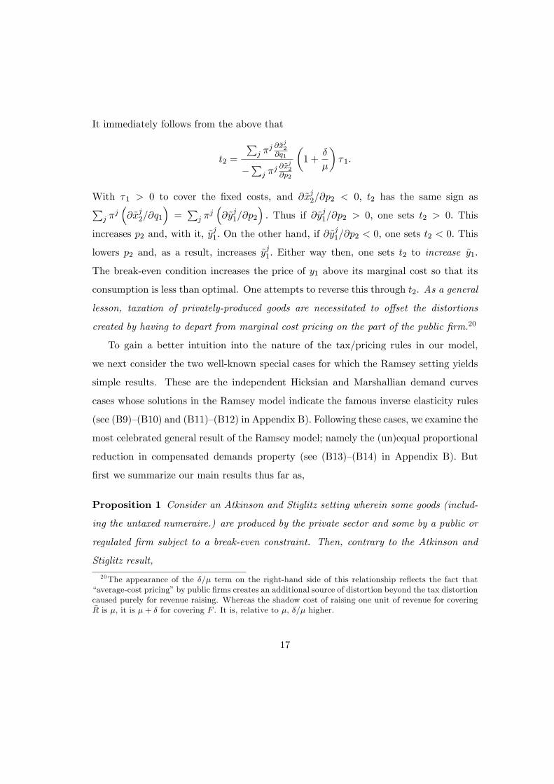
It immediately follows from the above that

t2 =

∑j π

j ∂xj2

∂q1

−∑

j πj ∂x

j2

∂p2

(1 +

δ

µ

)τ1.

With τ1 > 0 to cover the fixed costs, and ∂xj2/∂p2 < 0, t2 has the same sign as∑j π

j(∂xj2/∂q1

)=∑

j πj(∂yj1/∂p2

). Thus if ∂yj1/∂p2 > 0, one sets t2 > 0. This

increases p2 and, with it, yj1. On the other hand, if ∂y

j1/∂p2 < 0, one sets t2 < 0. This

lowers p2 and, as a result, increases yj1. Either way then, one sets t2 to increase y1.

The break-even condition increases the price of y1 above its marginal cost so that its

consumption is less than optimal. One attempts to reverse this through t2. As a general

lesson, taxation of privately-produced goods are necessitated to offset the distortions

created by having to depart from marginal cost pricing on the part of the public firm.20

To gain a better intuition into the nature of the tax/pricing rules in our model,

we next consider the two well-known special cases for which the Ramsey setting yields

simple results. These are the independent Hicksian and Marshallian demand curves

cases whose solutions in the Ramsey model indicate the famous inverse elasticity rules

(see (B9)—(B10) and (B11)—(B12) in Appendix B). Following these cases, we examine the

most celebrated general result of the Ramsey model; namely the (un)equal proportional

reduction in compensated demands property (see (B13)—(B14) in Appendix B). But

first we summarize our main results thus far as,

Proposition 1 Consider an Atkinson and Stiglitz setting wherein some goods (includ-

ing the untaxed numeraire.) are produced by the private sector and some by a public or

regulated firm subject to a break-even constraint. Then, contrary to the Atkinson and

Stiglitz result,

20The appearance of the δ/µ term on the right-hand side of this relationship reflects the fact that“average-cost pricing”by public firms creates an additional source of distortion beyond the tax distortioncaused purely for revenue raising. Whereas the shadow cost of raising one unit of revenue for coveringR is µ, it is µ+ δ for covering F . It is, relative to µ, δ/µ higher.

17

(i) Commodity taxes are desirable. Optimal commodity taxes are characterized by

(15).

(ii) Break-even constraints for public/regulated firms have spill overs to other goods;

they should be taxed too. These taxes are necessitated to offset the distortions created

by having to depart from marginal cost pricing on the part of the public firm.

(iii) The tax/pricing rules for both types of goods, those that are produced privately

and those that are provided through the public firm, are not affected by redistribution

concerns.

4 Constrained Pareto effi cient pricing rules

4.1 Zero cross-price compensated elasticities

Assume that Hicksian demands are independent so that the compensated demand of

any produced good does not depend on the prices of the other produced goods. In this

case, the reduced Slutsky matrix (where the line and column pertaining to leisure is

deleted) is diagonal so that equation (15) simplifies to

t2...tn(

1 + δµ

)τ1

...(1 + δ

µ

)τm

=δ

µ

0...0∑j π

jyj1

−∑j π

j∂yj1

∂q1...∑

j πjyjm

−∑j π

j ∂yjm

∂qm

.

Consequently, for all i = 2, . . . , n and s = 1, 2, . . . ,m,

ti = 0,

τ s =δ

µ+ δ

∑j π

jyjs

−∑

j πj ∂y

js

∂qs

=δ

µ+ δ

qs∑

j πjyjs∑

j πj yjs ε

jss

,

18

where εjss is the absolute value of the j-type’s own-price elasticity of compensated de-

mand for ys. Or, for all i = 2, . . . , n and s = 1, 2, . . . ,m, ti = 0 and

τ s1 + τ s

=δ∑

j πjyjs

(µ+ δ)∑

j πjyjs ε

jss

, (16)

which is an inverse elasticity rule. Again, the inverse elasticity rule arises only because

of the existence of the break-even constraint. In the absence of this constraint, δ = 0 so

that τ s, for all s = 1, 2, . . . ,m, will also be equal to zero.

The next question concerns the difference between our results of t = 0 and τ charac-

terized by equation (16) with the inverse elasticity rules derived in the Ramsey frame-

work (with a break-even constraint). The corresponding results under linear income

taxes with independent Hicksian demands are reported in equations (B9)—(B10) in Ap-

pendix B. Comparing the two sets of results reveals two differences. One is that whereas

in the traditional Ramsey model, both types of goods are subject to the inverse elastic-

ity rules, in the Atkinson-Stiglitz framework only the goods that are produces by public

firms are subject to the inverse elasticity rule. The goods produced by private firms

should not be taxed. The second difference is that in the traditional Ramsey frame-

work, the inverse elasticity rules are adjusted for redistributive concerns (through the

covariance terms). No such terms appear in the Atkinson-Stiglitz framework. Here are

redistributive concerns are taken care of by nonlinear income taxes. The only role for

commodity taxes is “effi ciency”. There will be no tax on private goods while the goods

provided by the public form are subject to the inverse elasticity rule that reflect pure

effi ciency considerations; see equation (16).

To sum, we find that in this special case, the private goods (not included in the

break-even constraint) continue to go untaxed as in the Atkinson-Stiglitz setting with no

break-even constraint. On the other hand, the pricing rules used by the public firm are

purely effi ciency-driven Ramsey rules. Goods are taxed inversely to their compensated

demand elasticity regardless of their distributional implications. Redistribution is taken

19

care of by the income tax allowing the public firm’s prices to be adjusted for revenue

raising (as in the Ramsey model with identical individuals).

It will become clear below that the apparent simplicity of this rule is to some extent

misleading. It obscures some effects which are present but happen to cancel out in this

special case. We shall return to this issue in the next subsections.

4.2 Zero cross-price elasticities

We now turn to the case where Marshallian demand functions are independent so that

the demand for any given good does not depend on the prices of other (produced)

goods.21 To simplify the pricing rules that obtain in this case, it is simpler to start

from the intermediate expressions (A10)—(A11) given in Appendix A rather than from

(15). Rearranging these expressions, making use of the weak-separability assumption,

and setting all the cross-price derivatives equal to zero, we obtain for all i = 2, . . . , n

and s = 1, 2, . . . ,m,

ti∑j

πj∂xji∂pi

+∑j

πjxji

n∑e=1

te∂xje∂cj

+

(1 +

δ

µ

) m∑f=1

τ f∂yjf∂cj

= 0, (17)

(1 +

δ

µ

)τ s∑j

πj∂yjs∂qs

+∑j

πjyjs

n∑e=1

te∂xje∂cj

+

(1 +

δ

µ

) m∑f=1

τ f∂yjf∂cj

+δ

µ

∑j

πjyjs = 0.

(18)

Before simplifying these expressions any further, it is informative to delve into their

interpretation. Recall that we are considering a compensated variation in the tax rates

such that dcj = xjidti for a variation in ti and dcj = yjsdqs for a variation in τ s. In other

words, individual disposable incomes are adjusted to keep utility levels constant for all

individuals. With utility levels unchanged, the impact of the variation on social welfare

entirely depends on the extra tax revenue (or profit) it generates. The left-hand sides21Much of the regulation and industrial organization literature uses quasi-linear preference. In that

case there are no income effects and the distinction between Hicksian and Marshallian demand becomesirrelevant.

20

of (17)—(18) measure the social value of this extra tax revenue (for a variation in ti or

in τ s respectively). Obviously, when the tax system is optimized, this social value must

be equal to zero (otherwise welfare could be increased by changing the tax rates).

To understand this interpretation, assume one changes cj after ti or τ s changes.

Start with a variation in ti. With the tax revenues being given by

∑j

πj

n∑e=1

texje +

m∑f=1

τ fyjf

,

and the cross-price derivatives being equal to zero, the change in ti produces an extra

tax revenue of ∑j

πjxji + ti∑j

πj∂xji∂pi

.

Our compensation rule requires∑

j πjxji of this to be rebated to individuals.

22 The net

change in revenue, minus compensation, is equal to

ti∑j

πj∂xji∂pi

.

This is the first expression on the left-hand side of (17). At the same time, the∑

j πjxji

compensation leads to an additional tax revenue of

n∑e=1

texje

∑j

πjxji

+

m∑f=1

τ fyjf

∑j

πjxji

=

∑j

πjxji

n∑e=1

texje +

m∑f=1

τ fyjf

.

To convert these tax revenue changes into social welfare (measured in units of general

revenues), one must multiply tax revenue variations emanating from y-goods by a factor

of (1 + δ/µ). This is because the revenue from y-goods enters both the global govern-

ment budget constraint as well as the break-even constraint. This results in the second

expression on the left-hand side of (17).

22To see this, observe that cj changes according to dcj = xjidti so that aggregate compensations

change by∑

j πjdcj =

(∑j π

jxji

)dti.

21

The left-hand side of (18) can be decomposed in a similar way, except for one extra

complication; namely the additional term (δ/µ)∑

j πjyjs. In this exercise,

∑j π

jyjs rep-

resents the value of the refunds to individuals. When collected as a tax, this amount has

a social value of (1+δ/µ)∑

j πjyjs. On the other hand, the refund “costs”only

∑j π

jyjs

(it comes from the general budget and has no impact on the break even constraint).

To ease the comparison with traditional Ramsey expressions, we can rewrite (17)—

(18) as inverse elasticity rules. Introducing

Ai =H∑j=1

πjxji

n∑e=1

te∂xje∂cj

+

(1 +

δ

µ

) m∑f=1

τ f∂yjf∂cj

, (19)

Bs =H∑j=1

πjyjs

n∑e=1

te∂xje∂cj

+

(1 +

δ

µ

) m∑f=1

τ f∂yjf∂cj

+δ

µ

∑j

πjyjs, (20)

where Ai and Bs measure the social value of the extra tax revenues due to refunds, with

Bs also including (δ/µ)∑

j πjyjs. We have, for all i = 2, . . . , n and s = 1, 2, . . . ,m,

ti1 + ti

=Ai∑

j πjxjiη

jii

, (21)

τ s1 + τ s

=Bs

(1 + δ/µ)∑

j πjyjsε

jss

, (22)

where and ηjii and εjss denote the absolute value of the j-type’s own-price elasticity of

Marshallian demands for xi and ys.

Expressions (21)—(22) have a number of interesting implications, particularly when

compared to their traditional counterparts. First, the effect of the break-even constraint

is no longer confined to the goods which enter this constraint. Instead, it spills over to the

other goods which no longer go untaxed (compare with the result obtained in Subsection

4.1). Second, we get inverse elasticity rules as in the Ramsey model; albeit without

redistributive terms. This becomes clear below. The numerator of both expressions

contain the “tax revenue”terms Ai and Bs. Recall that these expressions measure the

22

social value of the extra tax revenue generated from the demand variations that follow

the (compensating) adjustments in disposable income.

One may wonder why these terms were absent in Subsection 4.1. The key to under-

standing this property is that when Hicksian demands are independent, the price-cum-

income variations we consider have by definition no impact on the demand of any of the

other goods. And the effect on the good under consideration is already captured in the

(compensated) elasticity term. To sum up, Subsection 4.1 has given simple results, not

because the different effects were absent but because they happen to cancel out exactly

under the considered assumptions.

Finally, compare (21)—(22) with their counterparts in the traditional Ramsey model

under linear income taxes and independent Marshallian demands, as reported by (B11)—

(B12) in Appendix B. The comparison reveals one significant difference. Our model

results in the same exact expressions for optimal tax rates with one exception. Ex-

pressions (21)—(22) contain no terms reflecting redistributive concerns. These concerns

enter in the Ramsey model through the covariance terms in (B11)—(B12).

4.3 Proportional reduction in compensated demands

When there are cross-price effects, the Ramsey model no longer yields results that can

be presented as simple inverse elasticity rules. One popular way to present the tax rules

in this case is in terms of proportional reduction in compensated demands. This leads to

the celebrated “equal proportional reduction”pure effi ciency result in the one-consumer

Ramsey problem (and adjusted for redistributive considerations in the many household

case).

23

−

∑ne=1 te

(∑j π

j ∂xji

∂pe

)+∑m

f=1 τ f

(∑j π

j ∂xji

∂qf

)∑

j πjxji

=δ

µ

∑mf=1 τ f

(∑j π

j ∂yjf

∂pi

)∑

j πjxji

, (23)

−

∑ne=1 te

(∑j π

j ∂yjs

∂pe

)+∑m

f=1 τ f

(∑j π

j ∂yjs

∂qf

)∑

j πjyjs

=δ

µ+δ

µ

∑mf=1 τ f

(∑j π

j ∂yjf

∂qs

)∑

j πjyjs

.

(24)

The left-hand side of (23) and (24) represents the proportional reduction in compensated

demand of xi and yi respectively. More precisely, it is proportional to the compensated

impact of the considered good’s tax rate on the break-even constraint. And as such, it

differs across different commodities. Consequently, a version of the inverse elasticity rule

also holds in the Atkinson-Stiglitz framework with a break-even constraint. However,

the reduction is adjusted for tax revenue considerations; or more precisely the revenue

of the regulated firm.

These are to be compared with (B13) and (B14) given in Appendix B for the Ramsey

model. One again immediately observes that the two sets of formulas are identical except

for the covariance terms that appear in (B13)—(B14). Equations (23) and (24) contain

no such redistributive terms. Consequently, as in Subsection 4.2, nonlinear income

taxation fully takes care of redistributive concerns and obviates the need to adjust the

inverse elasticity rules for redistribution. We summarize the main results of this section

as,

Proposition 2 In the Atkinson and Stiglitz setting of Proposition 1:

(i) Assume compensated demands are independent. Then, (a) the goods that are

produced by non-regulated firms should not be taxed but public/regulated firms’ goods

should be. (b) Taxation of public/regulated firms’goods follow the Ramsey inverse elas-

ticity rule as characterized by equation (16). (c) The taxation/pricing rules are purely

effi ciency-driven. Redistribution is taken care of by the income tax allowing the public

24

firm’s prices to be adjusted for revenue raising (as in the Ramsey model with identical

individuals).

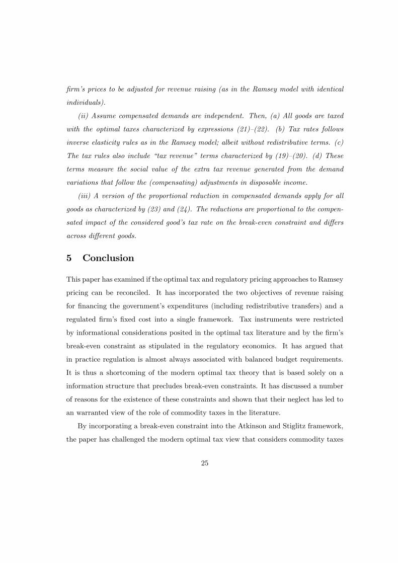
(ii) Assume compensated demands are independent. Then, (a) All goods are taxed

with the optimal taxes characterized by expressions (21)—(22). (b) Tax rates follows

inverse elasticity rules as in the Ramsey model; albeit without redistributive terms. (c)

The tax rules also include “tax revenue” terms characterized by (19)—(20). (d) These

terms measure the social value of the extra tax revenue generated from the demand

variations that follow the (compensating) adjustments in disposable income.

(iii) A version of the proportional reduction in compensated demands apply for all

goods as characterized by (23) and (24). The reductions are proportional to the compen-

sated impact of the considered good’s tax rate on the break-even constraint and differs

across different goods.

5 Conclusion

This paper has examined if the optimal tax and regulatory pricing approaches to Ramsey

pricing can be reconciled. It has incorporated the two objectives of revenue raising

for financing the government’s expenditures (including redistributive transfers) and a

regulated firm’s fixed cost into a single framework. Tax instruments were restricted

by informational considerations posited in the optimal tax literature and by the firm’s

break-even constraint as stipulated in the regulatory economics. It has argued that

in practice regulation is almost always associated with balanced budget requirements.

It is thus a shortcoming of the modern optimal tax theory that is based solely on a

information structure that precludes break-even constraints. It has discussed a number

of reasons for the existence of these constraints and shown that their neglect has led to

an warranted view of the role of commodity taxes in the literature.

By incorporating a break-even constraint into the Atkinson and Stiglitz framework,

the paper has challenged the modern optimal tax view that considers commodity taxes

25

redundant. It has restored many of the earlier Ramsey tax/pricing lessons within the

Atkinson and Stiglitz framework. In particular, it has shown that while nonlinear income

taxes does take care of all redistributive concerns, this does not mean that commodity

taxes are redundant. Break-even constraints create a role for commodity taxes. Inter-

estingly too, this role goes beyond taxation of goods produced by the public/regulated

firm but to the taxation of other goods as well. Put differently, break-even constraints

for “regulated goods”have spill overs to “non-regulated goods”.

We conclude by pointing out a number of possible extensions to our study. First,

it would be interesting to compare the spill-over effects on the prices of non-regulated

goods to the markups imposed on the goods subject to break-even constraints. Our

various expressions suggest that this depends mainly on the size of the (compensated)

cross-price effects. However, the complex way they operate does not allow one to draw

clearcut conclusions at this level of generality. Numerical examples could provide some

illustrative indications, while an empirical study may lead to more satisfactory answers.

Second, we have not formally modeled the informational asymmetries between public

authorities and the regulated firm. These have been at the heart of the regulatory

economics literature during the last two decades.23 Such asymmetries of information

would introduce an additional layer of complexity. For the regulator, the design of an

incentive schemes come on top (and is intertwined) with the traditional price pricing

problem; see e.g., Laffont and Tirole (1993, chapter 3). However, the use of sophisticated

incentive regulation does not in itself solve the problem of breaking even. In particular,

this literature uses Ramsey pricing as a benchmark which obtains under full information.

Under asymmetric information pertaining to a public/regulated firm’s cost, pricing rules

are more complex and often incorporate incentive corrections. As far as our results are

23As we have emphasized previously, our objective has been to explore what break-even constraintsimply for the role of commodity taxes however one rationalizes these constraints. In a way, this issomewhat akin to the one-consumer Ramsey tax problem wherein one rules out lump-sum taxation fora variety of reasons and studies its implications for the design of optimal commodity taxes.

26

concerned, this complexity can only reinforce our main findings. The use of Ramsey-

type prices in the Atkinson-Stiglitz setting, and the spillover to the taxation of goods

produced in the private sector, are expected to be robust. What may not be robust,

though, are the simple results we obtained for separable demands. However, even these

results may well continue to hold, at least in some circumstances. In particular, Laffont

and Tirole (1993, p. 173) show that when the cost function satisfies some separability

conditions, one obtains the so-called “incentive-pricing dichotomy”. Then, the incentive

design leaves the pricing rules unaffected and we return to traditional Ramsey pricing.

Last but not least, regulation often pursues specific and likely non-welfarist redis-

tributive objectives (as in universal access). It would be interesting to study how these

objectives interact with the general objectives of tax policy.

27

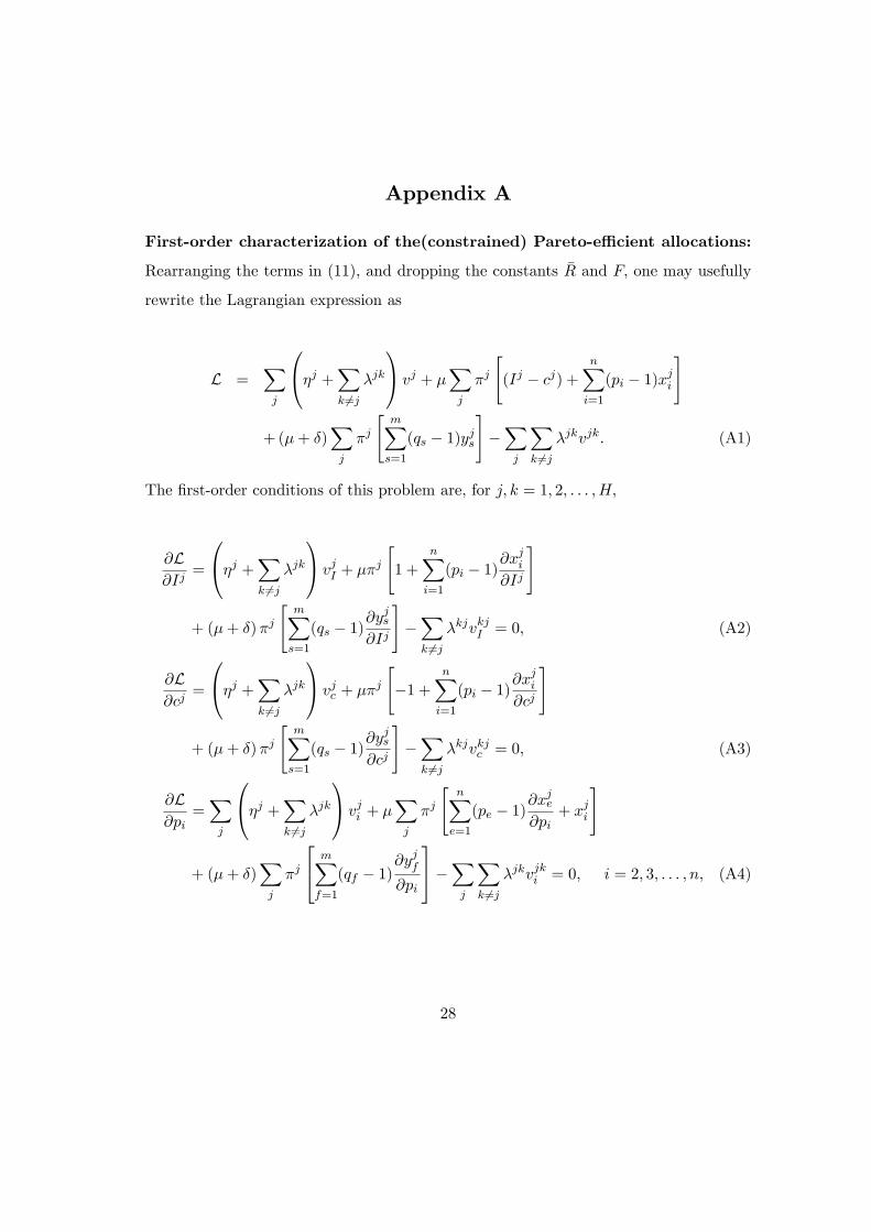
Appendix A

First-order characterization of the(constrained) Pareto-effi cient allocations:

Rearranging the terms in (11), and dropping the constants R and F, one may usefully

rewrite the Lagrangian expression as

L =∑j

ηj +∑k 6=j

λjk

vj + µ∑j

πj

[(Ij − cj) +

n∑i=1

(pi − 1)xji

]

+ (µ+ δ)∑j

πj

[m∑s=1

(qs − 1)yjs

]−∑j

∑k 6=j

λjkvjk. (A1)

The first-order conditions of this problem are, for j, k = 1, 2, . . . ,H,

∂L∂Ij

=

ηj +∑k 6=j

λjk

vjI + µπj

[1 +

n∑i=1

(pi − 1)∂xji∂Ij

]

+ (µ+ δ)πj

[m∑s=1

(qs − 1)∂yjs∂Ij

]−∑k 6=j

λkjvkjI = 0, (A2)

∂L∂cj

=

ηj +∑k 6=j

λjk

vjc + µπj

[−1 +

n∑i=1

(pi − 1)∂xji∂cj

]

+ (µ+ δ)πj

[m∑s=1

(qs − 1)∂yjs∂cj

]−∑k 6=j

λkjvkjc = 0, (A3)

∂L∂pi

=∑j

ηj +∑k 6=j

λjk

vji + µ∑j

πj

[n∑e=1

(pe − 1)∂xje∂pi

+ xji

]

+ (µ+ δ)∑j

πj

m∑f=1

(qf − 1)∂yjf∂pi

−∑j

∑k 6=j

λjkvjki = 0, i = 2, 3, . . . , n, (A4)

28

∂L∂qs

=∑j

ηj +∑k 6=j

λjk

vjs + µ∑j

πj

[n∑e=1

(pe − 1)∂xje∂qs

]

+ (µ+ δ)∑j

πj

m∑f=1

(qf − 1)∂yjf∂qs

+ yjs

−∑j

∑k 6=j

λjkvjks = 0, s = 1, 2, . . . ,m,

(A5)

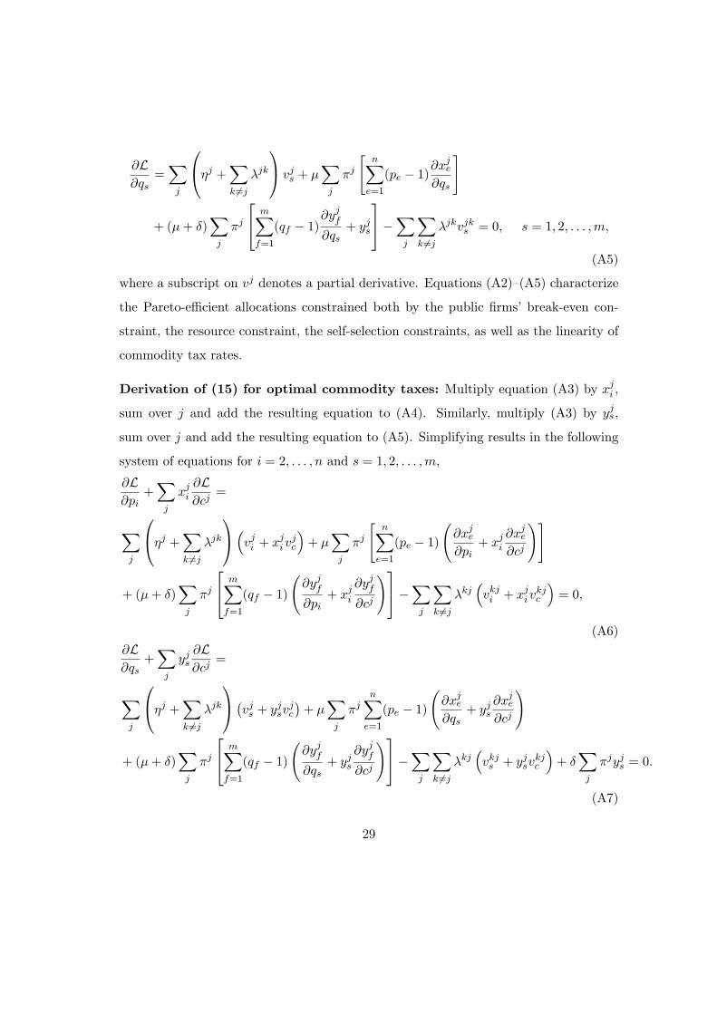
where a subscript on vj denotes a partial derivative. Equations (A2)—(A5) characterize

the Pareto-effi cient allocations constrained both by the public firms’break-even con-

straint, the resource constraint, the self-selection constraints, as well as the linearity of

commodity tax rates.

Derivation of (15) for optimal commodity taxes: Multiply equation (A3) by xji ,

sum over j and add the resulting equation to (A4). Similarly, multiply (A3) by yjs,

sum over j and add the resulting equation to (A5). Simplifying results in the following

system of equations for i = 2, . . . , n and s = 1, 2, . . . ,m,

∂L∂pi

+∑j

xji∂L∂cj

=

∑j

ηj +∑k 6=j

λjk

(vji + xjivjc

)+ µ

∑j

πj

[n∑e=1

(pe − 1)

(∂xje∂pi

+ xji∂xje∂cj

)]

+ (µ+ δ)∑j

πj

m∑f=1

(qf − 1)

(∂yjf∂pi

+ xji∂yjf∂cj

)−∑j

∑k 6=j

λkj(vkji + xjiv

kjc

)= 0,

(A6)∂L∂qs

+∑j

yjs∂L∂cj

=

∑j

ηj +∑k 6=j

λjk

(vjs + yjsvjc

)+ µ

∑j

πjn∑e=1

(pe − 1)

(∂xje∂qs

+ yjs∂xje∂cj

)

+ (µ+ δ)∑j

πj

m∑f=1

(qf − 1)

(∂yjf∂qs

+ yjs∂yjf∂cj

)−∑j

∑k 6=j

λkj(vkjs + yjsv

kjc

)+ δ

∑j

πjyjs = 0.

(A7)

29

With vji +xjivjc = 0 from Roy’s identity, the left-hand side of (A6) shows the impact

on the Lagrangian expression L of a variation in pi when the disposable income of

individuals is adjusted according to

dcj = xjidti, (A8)

to keep their utility levels constant. With vjs + yjsvjc = 0, the left-hand side of (A7)

shows the same compensated effect for a variation in qs where

dcj = yjsdτ s. (A9)

These compensated derivatives, (∂L/∂pi)vj=vj and (∂L/∂qs)vj=vj vanish at the optimal

solution.

Make use of Roy’s identity to set,

vji + xjivjc = 0,

vkji + xkji vkjc = 0,

vjs + yjsvjc = 0,

vkjs + ykjs vkjc = 0.

Substitute these values in equations (A6)—(A7), set pi−1 = ti and qs−1 = τ s, and divide

by µ. Upon changing the order of summation and further simplification one arrives at,

for all i = 2, . . . , n, and s = 1, 2, . . . ,m,

n∑e=1

te

∑j

πj

(∂xje∂pi

+ xji∂xje∂cj

)+

(1 +

δ

µ

) m∑f=1

τ f

∑j

πj

(∂yjf∂pi

+ xji∂yjf∂cj

)− 1

µ

∑j

∑k 6=j

λkj(xji − x

kji

)vkjc = 0, (A10)

n∑e=1

te

∑j

πj

(∂xje∂qs

+ yjs∂xje∂cj

)+

(1 +

δ

µ

) m∑f=1

τ f

∑j

πj

(∂yjf∂qs

+ yjs∂yjf∂cj

)− 1

µ

∑j

∑k 6=j

λkj(yjs − ykjs

)vkjc +

δ

µ

∑j

πjyjs = 0. (A11)

30

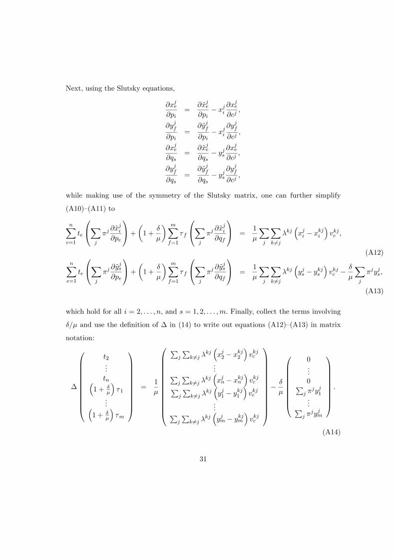
Next, using the Slutsky equations,

∂xje∂pi

=∂xje∂pi− xji

∂xje∂cj

,

∂yjf∂pi

=∂yjf∂pi− xji

∂yjf∂cj

,

∂xje∂qs

=∂xje∂qs− yjs

∂xje∂cj

,

∂yjf∂qs

=∂yjf∂qs− yjs

∂yjf∂cj

,

while making use of the symmetry of the Slutsky matrix, one can further simplify

(A10)—(A11) to

n∑e=1

te

∑j

πj∂xji∂pe

+

(1 +

δ

µ

) m∑f=1

τ f

∑j

πj∂xji∂qf

=1

µ

∑j

∑k 6=j

λkj(xji − x

kji

)vkjc ,

(A12)n∑e=1

te

∑j

πj∂yjs∂pe

+

(1 +

δ

µ

) m∑f=1

τ f

∑j

πj∂yjs∂qf

=1

µ

∑j

∑k 6=j

λkj(yjs − ykjs

)vkjc −

δ

µ

∑j

πjyjs,

(A13)

which hold for all i = 2, . . . , n, and s = 1, 2, . . . ,m. Finally, collect the terms involving

δ/µ and use the definition of ∆ in (14) to write out equations (A12)—(A13) in matrix

notation:

∆

t2...tn(

1 + δµ

)τ1

...(1 + δ

µ

)τm

=

1

µ

∑j

∑k 6=j λ

kj(xj2 − x

kj2

)vkjc

...∑j

∑k 6=j λ

kj(xjn − xkjn

)vkjc∑

j

∑k 6=j λ

kj(yj1 − y

kj1

)vkjc

...∑j

∑k 6=j λ

kj(yjm − ykjm

)vkjc

− δ

µ

0...0∑j π

jyj1...∑

j πjyjm

.

(A14)

31

Premultiplying through by ∆−1 yields

t2...tn(

1 + δµ

)τ1

...(1 + δ

µ

)τm

=

1

µ∆−1

∑j

∑k 6=j λ

kj(xj2 − x

kj2

)vkjc

...∑j

∑k 6=j λ

kj(xjn − xkjn

)vkjc∑

j

∑k 6=j λ

kj(yj1 − y

kj1

)vkjc

...∑j

∑k 6=j λ

kj(yjm − ykjm

)vkjc

− δ

µ∆−1

0...0∑j π

jyj1...∑

j πjyjm

.

(A15)

With weak-separability of preferences, equations (12)—(13) hold so that xjki = xki and

yjks = yks . It then follows immediately that the first vector on the right-hand side of

(A15) vanishes, reducing it to (15).

Derivation of (23)—(24): With weakly-separable preferences, one can rearrange

equations (A12)—(A13) as

−µn∑e=1

te

∑j

πj∂xji∂pe

− µ m∑f=1

τ f

∑j

πj∂xji∂qf

= δm∑f=1

τ f

∑j

πj∂yjf∂pi

,

−µn∑e=1

te

∑j

πj∂yjs∂pe

− µ m∑f=1

τ f

∑j

πj∂yjs∂qf

= δm∑f=1

τ f

∑j

πj∂yjf∂qs

+ δ∑j

πjyjs.

Then divide the first set of equations by µ∑

j πjxji and the second set of equations by

µ∑

j πjyjs. They will then be rewritten as (23)—(24).

32

Appendix B: The benchmark

The many-consumer Ramsey problem with a break-evenconstraint

An individual of type j now chooses x, y, and L to maximize his utility u = u(x, y, L

)subject to the budget constraint

∑i pixi +

∑s qsys = wj (1− θ)L + b, where θ is the

linear income tax rate and b is the uniform lump-sum rebate. The resulting demand

functions for x and y, and the supply function for L, for all i = 1, 2, . . . , n and s =

1, 2, . . . ,m, are denoted by xji = xi(p, q, wj (1− θ) , b

), yjs = ys

(p, q, wj (1− θ) , b

), and

Lj = L(p, q, wj (1− θ) , b

). Substituting in the utility function yields the indirect utility

function24

vj = v(p, q, wj (1− θ) , b

)≡ u

(x(p, q, wj (1− θ) , b

), y(p, q, wj (1− θ) , b

), L(p, q, wj (1− θ) , b

)).

Let πj denote the proportion of individuals of type j in the economy and consider a

utilitarian social welfare function of the form

H∑j=1

πjW(vj),

where W (·) is increasing, twice differentiable, and concave. The optimization problem

consists of maximizing∑

j πjW

(vj)with respect to p, q, b and subject to resource and

break-even constraints (8)—(9). Observe that with x, y and L being homogeneous of

24Separability of preferences does not simplify the characterization of the unconditional demand andindirect utility functions. If the utility function is separable and is written as U

(f(x, y), L), all one can

do is to write, for a given L, the consumer’s demand for x, y as functions of p, q and wj (1− θ)L + b.Then,

vj = U(f(x(p, q, wj (1− θ)L+ b

), y(p, q, wj (1− θ)L+ b

)), L).

However, optimization over L yields L = L(p, q, wj (1− θ) , b

). Consequently,

vj = v(p, q, wj (1− θ) , b

).

33

degree zero in p, q, wj (1− θ) and b, consumer prices are determined only up to a pro-

portionality factor. It is for this reason that we do not optimize over θ, setting it equal

to zero.

The Lagrangian expression associated with maximizing∑

j πjW

(vj)with respect

to p, q, b and subject to constraints (8)—(9) is represented by

L =∑j

πjW(vj)

+ µ

∑j

πj

[n∑i=1

(pi − 1)xji +m∑s=1

(qs − 1)yjs − b]− R− F

+δ

∑j

πj

[m∑s=1

(qs − 1)yjs

]− F

.

The first-order conditions of this problem are,

∂L∂b

=∑j

πj∂W

∂vj∂vj

∂b+ µ

∑j

πj

[−1 +

n∑i=1

(pi − 1)∂xji∂b

]+

(µ+ δ)∑j

πj

[m∑s=1

(qs − 1)∂yjs∂b

]= 0, (B1)

∂L∂pi

=∑j

πj∂W

∂vj∂vj

∂pi+ µ

∑j

πj

[xji +

n∑e=1

(pe − 1)∂xje∂pi

]+

(µ+ δ)∑j

πj

m∑f=1

(qf − 1)∂yjf∂pi

= 0, i = 1, 2, . . . , n, (B2)

∂L∂qs

=∑j

πj∂W

∂vj∂vj

∂qs+ µ

∑j

πj

[n∑e=1

(pe − 1)∂xje∂qs

]+

(µ+ δ)∑j

πj

yjs +m∑f=1

(qf − 1)∂yjf∂qs

= 0, s = 1, 2, . . . ,m. (B3)

34

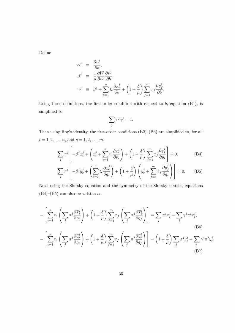
Define

αj ≡ ∂vj

∂b,

βj ≡ 1

µ

∂W

∂vj∂vj

∂b,

γj ≡ βj +

n∑e=1

te∂xje∂b

+

(1 +

δ

µ

) m∑f=1

τ f∂yjf∂b

.

Using these definitions, the first-order condition with respect to b, equation (B1), is

simplified to ∑j

πjγj = 1.

Then using Roy’s identity, the first-order conditions (B2)—(B3) are simplified to, for all

i = 1, 2, . . . , n, and s = 1, 2, . . . ,m,

∑j

πj

−βjxji +

(xji +

n∑e=1

te∂xje∂pi

)+

(1 +

δ

µ

) m∑f=1

τ f∂yjf∂pi

= 0, (B4)

∑j

πj

−βjyjs +

(n∑e=1

te∂xje∂qs

)+

(1 +

δ

µ

)yjs +m∑f=1

τ f∂yjf∂qs

= 0. (B5)

Next using the Slutsky equation and the symmetry of the Slutsky matrix, equations

(B4)—(B5) can also be written as

−

n∑e=1

te

∑j

πj∂xji∂pe

+

(1 +

δ

µ

) m∑f=1

τ f

∑j

πj∂xji∂qf

=∑j

πjxji −∑j

γjπjxji ,

(B6)

−

n∑e=1

te

∑j

πj∂yjs∂pe

+

(1 +

δ

µ

) m∑f=1

τ f

∑j

πj∂yjs∂qf

=

(1 +

δ

µ

)∑j

πjyjs −∑j

γjπjyjs.

(B7)

35

Finally, define

Ω ≡

∑j π

j ∂xj1

∂p1· · ·

∑j π

j ∂xj1

∂pn

∑j π

j ∂xj1

∂q1· · ·

∑j π

j ∂xj1

∂qm...

. . ....

.... . .

...∑j π

j ∂xjn

∂p1· · ·

∑j π

j ∂xjn

∂pn

∑j π

j ∂xjn

∂q1· · ·

∑j π

j ∂xjn

∂qm∑j π

j ∂yj1

∂p1· · ·

∑j π

j ∂yj1

∂pn

∑j π

j ∂yj1

∂q1· · ·

∑j π

j ∂yj1

∂qm...

. . ....

.... . .

...∑j π

j ∂yjm

∂p1· · ·

∑j π

j ∂yjm

∂pn

∑j π

j ∂yjm

∂q1· · ·

∑j π

j ∂yjm

∂qm

to rewrite equations (B6)—(B7) in matrix notation

Ω

t1...tn(

1 + δµ

)τ1

...(1 + δ

µ

)τm

=

∑Hj=1

(1− γj

)πjxj1

...∑Hj=1

(1− γj

)πjxjn∑H

j=1

(1 + δ

µ − γj)πjyj1

...∑Hj=1

(1 + δ

µ − γj)πjyjm

.

Pre-multiplying by Ω−1 yields,25

t1...tn(

1 + δµ

)τ1

...(1 + δ

µ

)τm

= Ω−1

∑Hj=1

(1− γj

)πjxj1

...∑Hj=1

(1− γj

)πjxjn∑H

j=1

(1 + δ

µ − γj)πjyj1

...∑Hj=1

(1 + δ

µ − γj)πjyjm

. (B8)

Observe that while the structure of taxes on private goods and public firms’goods

are not identical here, the same Ramsey tax/pricing rules apply to both under this

setting (as compared to our result in the text given by equation (15)). Observe also

that the many-consumer Ramsey problem we have considered as our benchmark here

allows for a uniform lump-sum rebate, b. The literature considers this problem for both

25As with ∆, Ω is of full rank so that its inverse exists; see Takayama (1985).

36

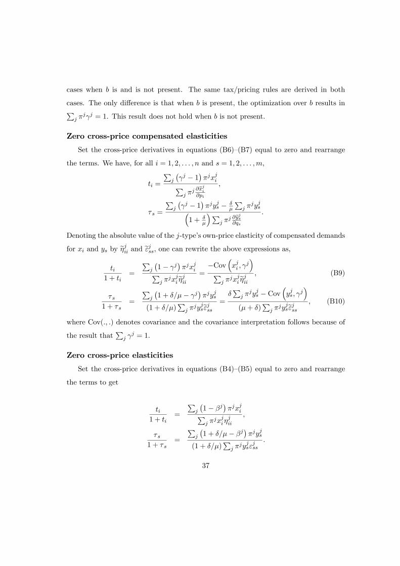
cases when b is and is not present. The same tax/pricing rules are derived in both

cases. The only difference is that when b is present, the optimization over b results in∑j π

jγj = 1. This result does not hold when b is not present.

Zero cross-price compensated elasticities

Set the cross-price derivatives in equations (B6)—(B7) equal to zero and rearrange

the terms. We have, for all i = 1, 2, . . . , n and s = 1, 2, . . . ,m,

ti =

∑j

(γj − 1

)πjxji∑

j πj ∂x

ji

∂pi

,

τ s =

∑j

(γj − 1

)πjyjs − δ

µ

∑j π

jyjs(1 + δ

µ

)∑j π

j ∂yjs

∂qs

.

Denoting the absolute value of the j-type’s own-price elasticity of compensated demands

for xi and ys by ηjii and ε

jss, one can rewrite the above expressions as,

ti1 + ti

=

∑j

(1− γj

)πjxji∑

j πjxji η

jii

=−Cov

(xji , γ

j)

∑j π

jxji ηjii

, (B9)

τ s1 + τ s

=

∑j

(1 + δ/µ− γj

)πjyjs

(1 + δ/µ)∑

j πjyjs ε

jss

=δ∑

j πjyjs − Cov

(yjs, γj

)(µ+ δ)

∑j π

jyjs εjss

, (B10)

where Cov(., .) denotes covariance and the covariance interpretation follows because of

the result that∑

j γj = 1.

Zero cross-price elasticities

Set the cross-price derivatives in equations (B4)—(B5) equal to zero and rearrange

the terms to get

ti1 + ti

=

∑j

(1− βj

)πjxji∑

j πjxjiη

jii

,

τ s1 + τ s

=

∑j

(1 + δ/µ− βj

)πjyjs

(1 + δ/µ)∑

j πjyjsε

jss

.

37

Add and subtract γj to βj to rewrite the above expressions as

ti1 + ti

=

∑j

(γj − βj

)πjxji −

∑j

(γj − 1

)πjxji∑

j πjxjiη

jii

,

τ s1 + τ s

=

∑j

(γj − βj

)πjyjs + (δ/µ)

∑j π

jyjs −∑

j

(γj − 1

)πjyjs

(1 + δ/µ)∑

j πjyjsε

jss

.

Finally, rewrite∑

j

(γj − 1

)πjxji and

∑j

(γj − 1

)πjyjs as Cov

(xji , γ

j)and Cov

(yjs, γj

).

Then recall from the definition of γj that we have: γj − βj =∑n

e=1 te

(∂xje/∂b

)+

(1 + δ/µ)∑m

f=1 τ f

(∂yjf/∂b

). Substitute in above and make use of the definitions of Ai

and Bs in the text to arrive at the counterparts of (21)—(22) in the text. We have, for

all i = 1, 2, . . . , n and s = 1, 2, . . . ,m,

ti1 + ti

=Ai − Cov

(xji , γ

j)

∑j π

jxjiηjii

, (B11)

τ s1 + τ s

=Bs − Cov

(yjs, γj

)(1 + δ/µ)

∑j π

jyjsεjss

. (B12)

Proportional reduction in compensated demands

Rearrange equations (B6)—(B7) and substitute −Cov(xji , γ

j)for∑

j

(1− γj

)πjxji

and −Cov(yjs, γj

)for∑

j

(1− γj

)πjyjs in them. We get, as counterparts of equations

(23)—(24) in the text,

−

∑ne=1 te

(∑j π

j ∂xji

∂pe

)+∑m

f=1 τ f

(∑j π

j ∂xji

∂qf

)∑

j πjxji

=

δµ

∑mf=1 τ f

(∑j π

j ∂yjf

∂pi

)− Cov

(xji , γ

j)

∑j π

jxji,

(B13)

−

∑ne=1 te

(∑j π

j ∂yjs

∂pe

)+∑m

f=1 τ f

(∑j π

j ∂yjs

∂qf

)∑

j πjyjs

=δ

µ+

δµ

∑mf=1 τ f

(∑j π

j ∂yjf

∂qs

)− Cov

(yjs, γj

)∑

j πjyjs

.

(B14)

38

References

[1] Allais, Maurice, 1947. Le problème de la coordination des transports et la théorieeconomique, Bulletin des Ponts et Chaussées et des Mines.

[2] Atkinson, Anthony B. and Joseph E. Stiglitz, 1976. The design of tax structure:direct versus indirect taxation, Journal of Public Economics, 6, 55—75.

[3] Baumol, William J. and David F. Bradford, 1970. Optimal departures from mar-ginal cost pricing, American Economic Review, 60, 265—283.

[4] Boiteux, Marcel, 1956. Sur la gestion des monopoles publics astreints à l’équilibrebudgétaire, Econometrica, 24, 22—40. Published in English as: On the manage-ment of public monopolies subject to budgetary constraints, Journal of EconomicTheory, 3, 219—240, 1971.

[5] Brown, Stephen and David Sibley, 1986. The Theory of Public Utility Pricing,Cambridge University Press, Cambridge, UK.

[6] Christiansen, Vidar, 1984. Which commodity taxes should supplement the incometax? Journal of Public Economics, 24, 195—220.

[7] Coase, Ronald, 1945. Price and output policy of state enterprise, Economics Jour-nal, 55, 112—113.

[8] Coase, Ronald, 1946. The marginal cost controversy, Economica, 13, 169—182

[9] Cremer, Helmuth and Firouz Gahvari, 1995. Uncertainty, optimal taxation and thedirect versus indirect tax controversy, Economic Journal, 105, 1165—79.

[10] Cremer, Helmuth and Firouz Gahvari, 1997. In—kind transfers, self—selection andoptimal tax policy. European Economic Review, 41, 97—114.

[11] Cremer, Helmuth and Firouz Gahvari, 1998. On optimal taxation of housing”,Journal of Urban Economics, 43, 315—335.

[12] Cremer, Helmuth and Firouz Gahvari, 2002. Nonlinear pricing, redistribution andoptimal tax policy, Journal of Public Economic Theory, 4, 139—161.

[13] Cremer, Helmuth, Firouz Gahvari and Norbert Ladoux, 1998. Externalities andoptimal taxation, Journal of Public Economics, 70, 343—364.

39

[14] Cremer, Helmuth, Fahrid Gasmi, André Grimaux and Jean-Jacqaues Laffont, 2001.Universal Service: an economic perspective, Annals of Public and Cooperative Eco-nomics, 72, 5—43.

[15] Cremer, Helmuth, Pierre Pestieau and Jean-Charles Rochet, 2001. Direct versusindirect taxation : The design of the tax structure revisited, International EconomicReview, 42, 781—799.

[16] Crew, Michael and Paul Kleindorfer, 2011. Competitive strategies under FMO andintermodal competition, in Reinventing the Postal Sector in an Electronic Age, M.A. Crew and P. R. Kleindorfer, ed., Northampton: Edward Elgar Publishing, Inc.,1—19.

[17] Crew, Michael and Paul Kleindorfer, 2012. Non-linear pricing and volume discountsand the USO under entry, in Multi-modal Competition and the Future of Mail, M.A. Crew and P. R. Kleindorfer, ed., Northampton: Edward Elgar Publishing, Inc.,1—18.

[18] Diamond, Peter A. and James A. Mirrlees, 1971. Optimal taxation and publicproduction I—II, American Economic Review, 61, 8—27, 261—278.

[19] Diamond, Peter A., 1975. A many-person Ramsey tax rule, Journal of Public Eco-nomics, 4, 335—342.

[20] Laffont, Jean-Jacques and Jean Tirole, 1990. Bypass and cream skimming, Amer-ican Economic Review, 80, 1042—1061.

[21] Laffont, Jean-Jacques and Jean Tirole, 1993. A Theory of Incentives in Procure-ment and Regulation, MIT Press, Cambridge, Mass.

[22] Laffont, Jean-Jacques and Jean Tirole, 2000. Competition in Telecommunications,MIT Press, Cambridge, Mass.

[23] Mirrlees, James A. 1971. An Exploration in the Theory of Optimum Income Tax-ation. Review of Economic Studies, 38, 175—208.

[24] Ramsey, Frank, 1927. A contribution to the theory of taxation, Economic Journal,37, 47—61.

[25] Sandmo, Agnar, 1976. Optimal taxation: An introduction to the literature, Journalof Public Economics, 6, 37—54.

40

[26] Stiglitz, Joseph E., 2015. In praise of Frank Ramsey’s contribution to the theoryof taxation. Economic Journal, 125, 235—268.

[27] Takayama, Akira. 1985. Mathematical Economics, 2nd ed. Cambridge: CambridgeUniversity Press.

[28] Viscusi, W. Kip, John Vernon and Joseph Harrington, 1998. Economics of Regula-tion and Antitrust, 2nd ed. MIT Press, Cambridge, MA.

[29] Vogelsang, Ingo et Jörg Finsinger, 1979. Regulatory adjustment process for optimalpricing of multiproduct firm, Bell Journal of Economics, 10, 157—171.

[30] Ware, Roger and Ralph A. Winter, 1986. Public pricing under imperfect competi-tion, International Journal of Industrial Organization, 4, 87—97.

41