The Ecological and Hydrological Significance of Ephemeral ...
RESTORING HYDROLOGICAL AND ECOLOGICAL FUNCTIONS OF
WETLANDS INVADED WITH REED CANARY GRASS (PHALARIS
ARUNDINACEA) FOR POTENTIAL OREGON SPOTTED FROG (RANA PRETIOSA)
OVIPOSITION RECOVERY AT JOINT BASE LEWIS-MCCHORD, FORT LEWIS,
WA
by
Pamela Abreu
A Thesis
Submitted in partial fulfillment of the requirements for the degree Master of Environmental Studies
The Evergreen State College June 2015

©2015 by Pamela Abreu. All rights reserved.

This Thesis for the Master of Environmental Studies Degree
by
Pamela Abreu
has been approved for
The Evergreen State College
by
________________________ Erin Martin, PhD.
Member of the Faculty
________________________ Date
ABSTRACT
Restoring Hydrological and Ecological Functions of Wetlands Invaded with Reed Canary Grass (Phalaris arundinacea) for Potential Oregon Spotted Frog (Rana pretiosa)
Oviposition Recovery at Joint Base Lewis-McChord, Fort Lewis, WA
Pamela Abreu
Reed canary grass (Phalaris arundinacea) is an invasive aquatic plant capable of changing wetland characteristics and outcompeting native species, causing wetland
habitat loss. One of the main causes of amphibian declines is loss of habitat. Currently the Oregon spotted frog (Rana pretiosa) is listed as threatened under the federal
Endangered Species Act, and wetland managers are making many efforts to restore its habitat. This research explored how reed canary grass (RCG) can be managed in order to restore Oregon spotted frog (OSF) oviposition habitat at the Joint Base Lewis-McChrod (JBLM), where an OSF translocation program is being conducted. Hydrologic (Water
depth and temperature), vegetation (Percent live RCG, percent RCG thatch cover, percent open water, emergent vegetation height, and RCG thatch height), and chemical (dissolved
oxygen and conductivity) measurements were collected at JBLM, where five different treatments were applied to wetlands invaded with RCG to reduce infestation. Results were compared to West Rocky Prairie (a successful OSF oviposition site). Treatments
applied at JBLM included: Mow/Burn/Herbicide, Mow/Burn, Mow/Herbicide, Burn/Herbicide, and a control treatment. 281 egg masses were found at West Rocky Prairie throughout 2015 oviposition season, and none at JBLM. Conductivity was
significantly higher at JBLM compared to West Rocky Prairie (Two sites at JBLM were 84.5 ± 7.4 and 89.7 ± 12.5, respectively; whereas West Rocky Prairie had a mean of 61.2
± 18.9), but it did not differed between treatments (SSamong= 773.126, p= 0.126) Dissolved oxygen did not significantly differed between sites (SSamong=
1.3498,p=0.9846). All hydrologic and vegetation variables (except for RCG thatch height) were affected by the different treatments. Chemical variables were not affected by
treatments. The treatment most successful at JBLM for OSF oviposition success was Mow/Herbicide. Nonetheless, more studies are needed to see if the lack of egg masses at JBLM is related to intrinsic habitat conditions, and it is recommended to study effects of herbicide at all stages for the Oregon spotted frog before using herbicide as a large-scale
management strategy.
Table of Contents
CHAPTER ONE: INTRODUCTION TO THESIS……………………………1
Introduction………………………………………………………………..1
CHAPTER TWO: LITERATURE REVIEW………………………………….4
Wetlands and Invasive Plants……………………………………………..4
Importance of Wetlands…………………………………………...4
Effects of Invasive Plants on Wetlands……………………………5
Reed Canary Grass in Washington Wetlands……………………………..7
Origin and Habitat………………………………………………...7
Basic Ecology……………………………………………………...8
Spread of RCG in Washington State………………………………9
Effects of RCG in Wetland Habitats……………………………..10
Control Practices………………………………………………...10
Mechanical Control Practices…………………………...11
Chemical Control Practices……………………………...12
Biological Control Practices…………………………….13
Other Methods…………………………………………...14
Control Practices Suitable for OSF Oviposition………...16
Effects on Amphibian populations……………………………….17
Oregon Spotted Frog in Washington…………………………………….17
Status……………………………………………………………..17
Life History………………………………………………………18
Habitat Needed for Oviposition………………………………….19
Effects of RCG on OSF…………………………………………..20
v
Management Strategies…………………………………………..21
CHAPTER THREE: METHODS……………………………………………..23
Study Areas………………………………………………………………23
Joint Base Lewis-McChord (JBLM)……………………………..24
West Rocky Prairie (WRP)……………………………………….26
Field Survey Methods: Vegetation Data…………………………………28
Joint Base Lewis-McChrod (JBLM)……………………………..29
West Rocky Prairie (WRP)……………………………………….30
Vegetation Monitoring…………………………………………...31
Field Survey Methods: Chemical and Hydrologic Data…………………31
Statistical Analysis……………………………………………………….33
CHAPTER FOUR: RESULTS………………………………………………...35
Site Differences…………………………………………………………..35
Egg Mass Data…………………………………………………...35
Chemical Data…………………………………………………...36
Hydrologic Data…………………………………………………39
Vegetation Differences Between Treatments…………………………....44
Percent Live RCG………………………………………………..44
Successful OSF Oviposition Habitat Characteristics……44
Unsuccessful OSF Oviposition Habitat Characteristics…45
Percent RCG Thatch Cover……………………………………...48
Successful OSF Ovipositon Habitat Characteristics…….48
Unsuccessful OSF Oviposition Habitat Characteristics…49
Percent Open Water……………………………………………...52
vi
Successful OSF Oviposition Habitat Characteristics……52
Unsuccessful OSF Oviposition Habitat Characteristics…53
Emergent Vegetation Height……………………………………..56
Successful OSF Oviposition Habitat Characteristics……56
Unsuccessful OSF Oviposition Habitat Characteristics…57 RCG Thatch Height………………………………………………60
Successful OSF Oviposition Habitat Characteristics……60
Unsuccessful OSF Oviposition Habitat Characteristics…61
CHAPTER FIVE: DISCUSSION……………………………………………...64
Site Differences…………………………………………………………..65
Egg Mass Data…………………………………………………...65
Chemical Data…………………………………………………...66
Hydrologic Data…………………………………………………68
Vegetation Differences Between Treatments……………………………70
Percent Live RCG………………………………………………..70
Percent RCG Thatch Cover……………………………………...71
Percent Open Water……………………………………………...72
Emergent Vegetation Height……………………………………..73
RCG Thatch Height………………………………………………74
Most Efficient Treatments for JBLM……………………………..75
CHAPTER SIX: RECOMMENDATIONS AND CONCLUSION………….77

v
List of Figures
Figure 1. Existing Oregon spotted frog populations in the State of Washington………...3
Figure 2. Map illustration of Reed canary grass distribution in Washington State………9
Figure 3. Map of Oregon spotted frog historical range………………………………….19
Figure 4. Map location of Watkins and Johnson within Joint Base Lewis-McChord, with corresponding positioning of treatment plots……………………………………………26
Figure 5. Map location of West Rocky Prairie in Western Washington………………...28
Figure 6. Map of setup of treated and control plots at the West area within West Rocky Prairie…………………………………………………………………………………….28
Figure 7. Placement of buffers and sub-plots within each existing treatment at Joint Base Lewis-McChord used for vegetation monitoring………………………………………...30
Figure 8. Image of constructed PVC structure used for data logger set-up at JBLM…...33
Figure 9. Image of installed data loggers at Joint Base Lewis-McChord……………….33
Figure 10: Mean conductivity for Johnson, Watkins, and West Rocky Prairie…………37
Figure 11: Mean dissolved oxygen concentrations for different treatments at Watkins and Johnson sites within Joint Base Lewis-McChord…………………………………...38
Figure 12: Mean surface water temperatures for different treatments at Watkins site within Joint Base Lewis-McChord………………………………………………………40
Figure 13: Mean surface water temperatures for different treatments at Johnson site within Joint Base Lewis-McChrod………………………………………………………40
Figure 14. Mean surface water temperatures at West Rocky Prairie site……………….41
Figure 15. Mean water depth for different treatments at Watkins site within Joint Base Lewis-McChord………………………………………………………………………….43
Figure 16. Mean water depth for different treatments at Johnson site within Joint Base Lewis-McChrod………………………………………………………………………….43
Figure 17. Mean water depth at West Rocky Prairie site………………………………..44

vi
Figure 18. Difference in average percent live reed canary grass per plot at West Rocky Prairie…………………………………………………………………………………….45
Figure 19. Difference in percent live reed canary grass per treatment for Watkins and Johnson sites within Joint Base Lewis-McChord………………………………………..47
Figure 20. Difference in percent reed canary grass thatch cover per plot at West Rocky Prairie…………………………………………………………………………………….49
Figure 21. Difference in percent reed canary grass thatch cover per treatment for Watkins and Johnson sites within Joint Base Lewis-McChord…………………………………...51
Figure 22. Difference in percent open water per plot at West Rocky Prairie…………...53
Figure 23. Difference in percent open water per treatment for Watkins and Johnson sites within Joint Base Lewis-McChord………………………………………………………55
Figure 24. Difference in mean emergent vegetation height per plot at West Rocky Prairie…………………………………………………………………………………….56
Figure 25. Difference in mean emergent vegetation height per treatment for Watkins and Johnson sites within Joint Base Lewis-McChord………………………………………..59
Figure 26. Difference in mean reed canary grass thatch height per plot at West Rocky Prairie…………………………………………………………………………………….60
Figure 27. Difference in mean reed canary grass thatch height per treatment for Watkins and Johnson sites within Joint Base Lewis-McChord…………………………………...62
vii
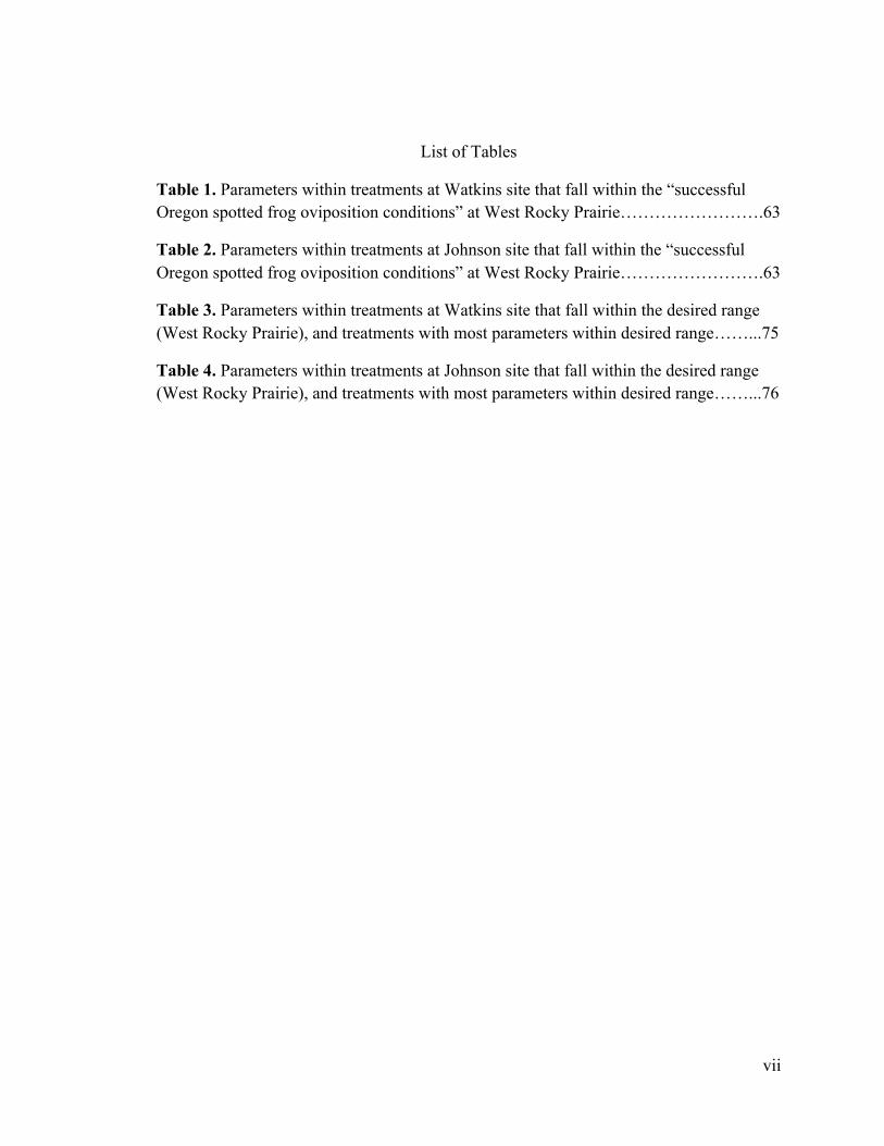
List of Tables
Table 1. Parameters within treatments at Watkins site that fall within the “successful Oregon spotted frog oviposition conditions” at West Rocky Prairie…………………….63
Table 2. Parameters within treatments at Johnson site that fall within the “successful Oregon spotted frog oviposition conditions” at West Rocky Prairie…………………….63
Table 3. Parameters within treatments at Watkins site that fall within the desired range (West Rocky Prairie), and treatments with most parameters within desired range……...75
Table 4. Parameters within treatments at Johnson site that fall within the desired range (West Rocky Prairie), and treatments with most parameters within desired range……...76

viii
Acknowledgements
This research was supported by the faculty of The Evergreen State College, notably: Dr. Erin Martin, Dr. Sarah Hamman, Dr. Dina Roberts, Dr. Kevin Francis, and the entire Science Support Center staff. In particular, I would like to thank my advisor, Dr. Erin Martin, for challenging me and motivating me throughout my time in the Master of Environmental Studies Program.
Thank you to Dr. Sarah Hamman, for supporting my ideas and helping direct me in the right direction throughout this thesis project, as well as lending me extra hands for the setup of my study. Thank you to Dr. Marc Hayes, for being a mentor throughout this entire process. Thank you to the Washington Department of Fish and Wildlife for giving me the opportunity to conduct my study within West Rocky Prairie Wildlife Area, the entire Joint Base Lewis-McChord Wildlife Division for allowing me the access and the opportunity to conduct my studies there. Thank you to the Center for Natural Lands Management (CNLM) for providing me with equipment necessary for this research, and Bill Grantham for supporting my ideas, providing guidance, and lending me a pair of extra hands whenever they were needed in the field. Thank you to Jim Mathieu for sharing the water data for West Rocky Prairie.
I would like to thank my family, especially my father, Roberto Abreu, for their unconditional love and support, even from a distance you are always with me. Thank you to Mr. Hutchinson, I couldn’t have done it without you.
1
CHAPTER 1: INTRODUCTION TO THESIS
Reed canary grass (Phalaris arundinacea) is an invasive aquatic plant that has
become a problem for ecosystem managers all across the Pacific Northwest. It is
considered an ecosystem engineer since it can spread, reproduce, and change wetland
characteristics. It is able to outcompete native species of plants due to its ability to
survive a wide range of environmental conditions (Kapust, McAllister, Hayes, & others,
2012). Reed canary grass (hereafter RCG), is a main cause of wetland habitat loss
(Lavergne & Molofsky, 2006), and habitat loss is considered one of the main causes for
amphibian declines worldwide (Denton & Richter, 2013; Petranka & Holbrook, 2006).
The Oregon spotted frog (Rana pretiosa) has been listed as a State Endangered
species in Washington since 1997, and just recently was listed as threatened under the
federal Endangered Species Act (Hallock, 2013; McAllister & Leonard, 1997). Several
human-related stressors have been suggested as the main cause of population declines of
Oregon spotted frog, including alteration and loss of wetland ecosystems, introduction of
non-native species, and changes in ultraviolet radiation and water chemistry (Kapust et
al., 2012; McAllister & Leonard, 1997).
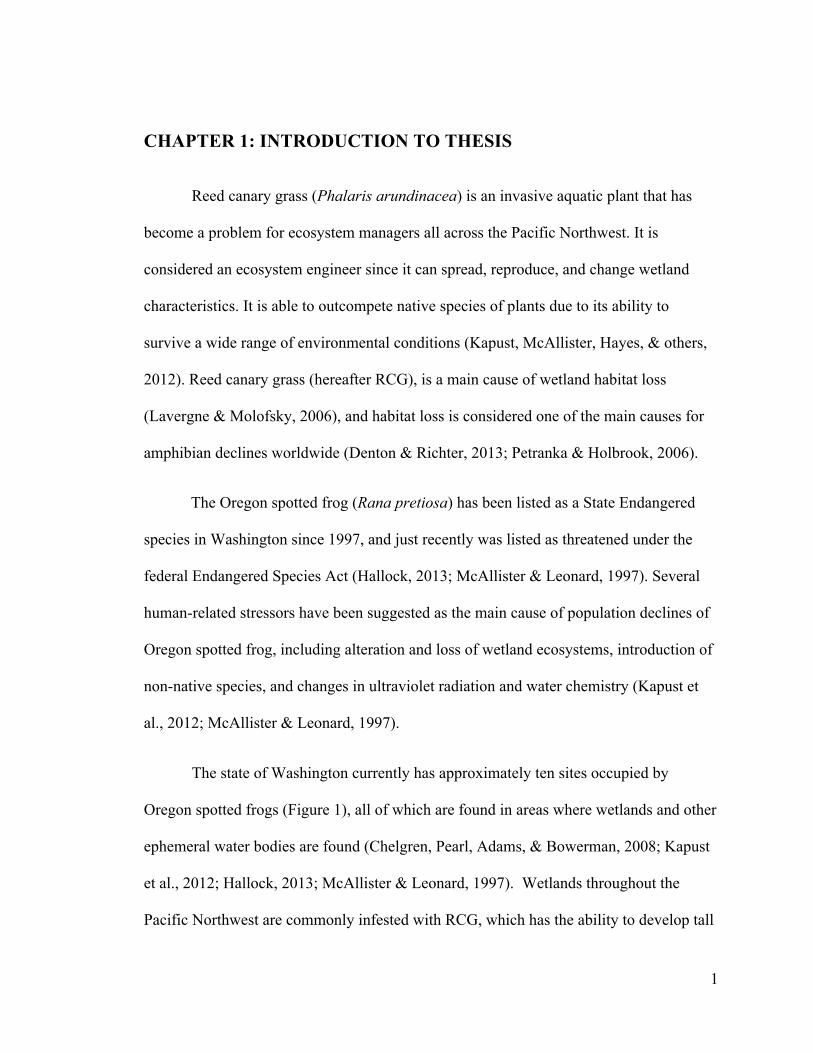
The state of Washington currently has approximately ten sites occupied by
Oregon spotted frogs (Figure 1), all of which are found in areas where wetlands and other
ephemeral water bodies are found (Chelgren, Pearl, Adams, & Bowerman, 2008; Kapust
et al., 2012; Hallock, 2013; McAllister & Leonard, 1997). Wetlands throughout the
Pacific Northwest are commonly infested with RCG, which has the ability to develop tall
2
monotypic stands that change the ecosystem structure and hydrology, as well as
eliminates low vegetation structure needed by the Oregon spotted frog (hereafter OSF) to
lay egg masses (Kapust et al., 2012). Studies by Kapust, McAllister and Hayes have
shown OSF tends to prefer sites where RCG has been treated in order to reduce its
density (Kapust et al., 2012).
This thesis was motivated by two different ongoing pilot studies being done at the
Joint Base Lewis McChord (JBLM). The pilot study, being done by Sarah Hamman with
the Center of Natural Lands Management (CNLM), consisting on assessing different
treatments to control RCG density within the wetlands found at the base. The second
pilot study consists of the implantation of an OSF population by relocating frogs from
two different populations (Conboy Lake and Black River) currently found in other areas
of Washington, in order to create a new population at JBLM. Most of the wetlands found
at the JBLM are infested with RCG, which can potentially affect the frog’s ability to lay
egg masses. This can inadvertently affect the frog’s ability to maintain a self-sustaining
the population. There is currently an example of a successful RCG treatment for OSF
oviposition success at West Rocky Prairie wildlife area (hereafter WRP), which is located
in Thurston County, where mowing desired areas has led to increased egg masses being
laid by OSF.
This study has several objectives: 1) to study how RCG can effectively be
controlled to improve wetland conditions for OSF oviposition habitat recovery at JBLM;
2) to see if RCG control treatments at JBLM can successfully replicate OSF oviposition
habitat; and 3) to learn about existing reed canary grass management techniques, and
which practices are the most efficient control of reed canary grass.
3
Figure 1:
Figure 1: Existing Oregon Spotted frog populations in the State of Washington (WDFW, 2013).
This study consists of a literature review that investigates wetlands and invasive
plants, RCG in Washington wetlands, treatment strategies for invasive RCG, and OSF in
Washington State. Later methodology, results, and discussion of results of my thesis
work are presented, followed by a final chapter that consists of my conclusion and
recommendations.
4
CHAPTER 2: LITERATURE REVIEW
The following literature review consists of looking at the importance of wetlands,
and how invasive plants are affecting these specific ecosystems. Then it looks
specifically Reed canary grass, including its life history and basic ecology, as well as its
current state in Washington, its effect on Washington wetlands, different available
control practices, and the effects it has on amphibian populations. Later it looks
specifically at the Oregon spotted frog and its status in the state of Washington, its life
history and basic ecology, habitat needed for oviposition, the effects of reed RCG has on
OSF, and management strategies being used in the state of Washington to restore OSF
populations.
WETLANDS AND INVASIVE PLANTS
Importance of wetlands
Wetlands around the country provide important habitat for a variety of native
flora, fauna, and waterfowl (Paveglio & Kilbride, 2000). Apart from providing habitat
and structure for wildlife, wetlands also provide water circulation services and help
regulate fire frequency regimes (Lavergne & Molofsky, 2006). Isolated wetlands provide
important habitat for amphibian populations. Currently, isolated wetlands (i.e.
hydrologically independent wetlands) are not considered critical habitat, and with human
population’s exponential growth many of these wetlands have been altered or lost
(Denton & Richter, 2013). The insufficient federal protection for isolated wetlands has
lead to the loss of breeding habitat for amphibians, since even small wetlands can

5
function as linkage habitats between isolated amphibian populations (Denton & Richter,
2013).
Effect of invasive plants on wetlands
Presently, many ecosystems around the world are being affected by non-native
biological species, and wetlands can be very sensitive to plant invaders (Lavergne &
Molofsky, 2006). Invasive plants are a significant wetland disruptor for biodiversity and
ecosystem functioning worldwide. The increased distribution and abundance of invasive
plant species is reducing biological diversity in wetlands, since they simplify plant
community structure, and change ecosystem processes leading to disturbance in nutrient
dynamics within the system (Schooler, McEvoy, & Coombs, 2006a).
Reductions in plant diversity can change wetland functions and services. The
effects of an invasive plant on the biotic community are dependent on the relative
abundance of the invasive acquired in the existing community (Schooler et al., 2006). Not
all invasive plants are over abundant, but each acts differently depending on the system
they are introduced to. An invasive plant is considered a “weak invader” if, after they
colonize, they stay at a relatively low abundance with minimal influence on other species,
therefore increasing species richness of the wetland ecosystem. However, when an
invasive plant increases in density to the point where most of the other species decrease,
it becomes a “strong invader,” and it can cause the extirpation of local species.
A simple equation can be used to explain the total impact of an invasive species,
where (I) is the impact an invader can have on the ecosystem, which depends on: the
6
abundance of the invader (A), the distribution of the invader within the wetland (D), and
the effect each invasive plant can have on the wetland ecosystem (or per capita effect)
(E); thus I= A x D x E (Schooler et al., 2006a).
The primary factor influencing diversity of wetland plant communities is the
duration of inundation periods within the wetland (hydrologic regime), since it can
promote or limit primary production. There will be a greater number of plant species
coexisting in a freshwater habitat that is seasonally flooded, since fluctuating water can
provide conditions desirable for a wide range of plant species. Variation in the
topography of the wetland, as well as fluctuation of moving water, creates fluctuations in
soil oxygen concentration. When water levels are high, the rate at which plant roots
obtain oxygen from the environment is slowed down, while also affecting seed
germination rates and photosynthetic ability. This happens because plant roots need
oxygen from the environment to respire, and standing water can prevent them from
accessing oxygen needed. Invasive aquatic plants have the ability to form dense stands
that can affect the hydrologic regime of a wetland by affecting water circulation regime
(Lavergne & Molofsky, 2006), as well as the plant diversity (Schooler et al., 2006a).
Plant diversity is an essential component of healthy wetland ecosystems, and
invasive aquatic plants have made maintaining a diverse plant community a challenge for
wetland managers. As invaders outcompete natives, invader abundance increases leading
to a decrease in plant diversity, which leads to further increase in invader abundance.
Maintaining the plant diversity in wetlands is crucial for wetland managers since it can
provide different niches for aquatic organisms, therefore increasing aquatic and wildlife
diversity (Hillhouse, Tunnell, & Stubbendieck, 2010). In the Pacific Northwest, invasive
7
RCG has been a major concern for wetland managers. Since RCG thrives in systems
where water is deeper, and inundation periods are extended (Miller & Zedler, 2003), it
can potentially infest habitat needed by the OSF for oviposition,
REED CANARY GRASS IN WASHINGTON WETLANDS
Origin and Habitat
RCG is native to Europe and Asia, but recently it has been disputed that it is also
native to North America, specifically the greater Interior Mountain West (Jakubowski,
Casler, & Jackson, 2010). Samples collected prior to 1900 suggest RCG could be native
to river systems in Montana, Idaho, and Wyoming. It is believed that the RCG that is
widely distributed now in the Pacific Northwest came from European cultivars, but both
native and introduced genotypes can occur (Miller & Zedler, 2003; Tu, 2004).
RCG is considered a wetland species since it is typically found in soils that are
nearly saturated or saturated through at least one growing season (Miller & Zedler, 2003).
Once this grass is established it can survive long periods of inundation. However, in order
to survive new establishment, periods of several months without standing water are
necessary to allow seeds to germinate (Fred Weinmann & United States. Army. Corps of
Engineers. Seattle District, 1984).

8
Basic Ecology
RCG is a cool-season perennial plant distributed extensively throughout the state
of Washington. It can reach up to 9 ft in height (2.7 m), with rough texture flat blades
8.9-25.4 cm long, and a width of 6.4 to 19.1 mm. This grass easily adapts to different
functions and modes of life, meaning it is able to live in a wide range of habitats and
utilize resources available. It also can easily develop into dense, monotypic stands.
Phalaris arundinacea has the ability to reproduce both vegetatively by its rhizome and
rhizome fragmentation, and sexually by seed dispersal (Paveglio & Kilbride, 2000).
RCG has the ability to establish and expand quickly since dense rhizome growth
occurs throughout one growing season, and seeds usually germinate directly after
ripening (Paveglio & Kilbride, 2000). This grass has the ability to form dense
monocultures because even though seeds have a short storage life, they can be easily
transported by air or water. This helps propagate the invasive and allows it to spread long
distances from its original location. Furthermore, monocultures can be formed due to the
plant’s quick growth and potential to release and propagate thousands of seeds at once.
The plant’s ability to spread vegetatively in a short period of time, grow
efficiently, tolerate multiple hydrological regimes, and serve as an ecosystem engineer by
changing the environment that surrounds it, makes reed canary grass a highly competitive
plant (Wilcox, Healy, & Zedler, 2007). For these reasons, RCG can have detrimental
impacts on structure of native plant and animal communities, and can alter multiple
ecosystem processes such as hydrology, nutrient cycling and fire regimes (Lavergne &
Molofsky, 2006). The ability of RCG to outcompete and have injurious effects on native
9
wetland communities is a main concern for wetland managers in the state of Washington,
leading to the current search for new and more efficient approaches to control the species.
Spread of reed canary grass (RCG) in Washington
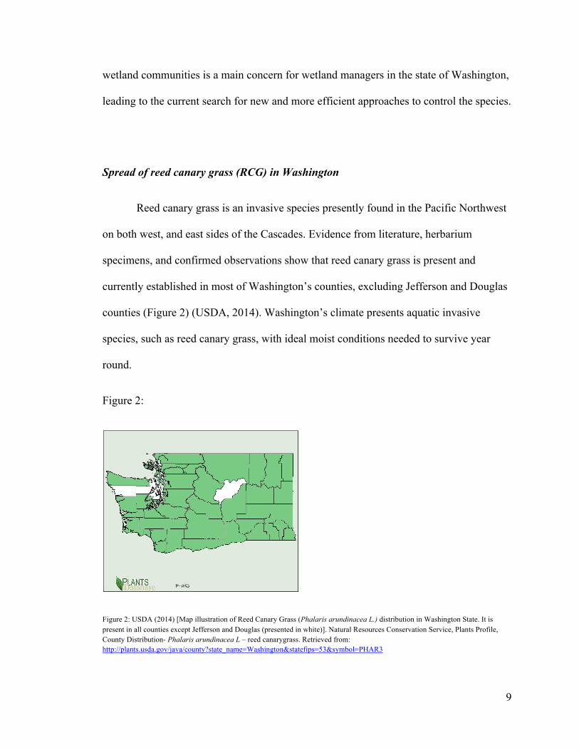
Reed canary grass is an invasive species presently found in the Pacific Northwest
on both west, and east sides of the Cascades. Evidence from literature, herbarium
specimens, and confirmed observations show that reed canary grass is present and
currently established in most of Washington’s counties, excluding Jefferson and Douglas
counties (Figure 2) (USDA, 2014). Washington’s climate presents aquatic invasive
species, such as reed canary grass, with ideal moist conditions needed to survive year
round.
Figure 2:
Figure 2: USDA (2014) [Map illustration of Reed Canary Grass (Phalaris arundinacea L.) distribution in Washington State. It is present in all counties except Jefferson and Douglas (presented in white)]. Natural Resources Conservation Service, Plants Profile, County Distribution- Phalaris arundinacea L – reed canarygrass. Retrieved from: http://plants.usda.gov/java/county?state_name=Washington&statefips=53&symbol=PHAR3
10
Effects of RCG on Wetland Habitats
RCG can alter the hydrology of wetland systems by trapping sediments, and
constricting water ways (Wisconsin Reed Canary Grass Management Working Group,
2009). It can affect water temperatures by restricting the amount of sunlight that can be in
contact with the water surface, cooling the water. This in turn can also affect surface
water depth, by avoiding water evaporation, and absorbing the water instead due to its
ability to develop adventitious roots at its nodes in response to flooding (Jenkins,
Yeakley, & Stewart, 2008)
Phalaris arundinacea is capable of altering nutrient dynamics within a wetland.
Since RCG homogenizes wetland habitats, and reduces environmental variability (which
has an effect on species richness) carbon sequestration capacity is decreased due to
acceleration of turnover periods (Wisconsin Reed Canary Grass Management Working
Group, 2009)
One of the most important alterations RCG has on wetland habitats is light
availability. Since it can turn wetlands into tall monocrops, it can prevent light from
reaching seedlings, which can crowd and limit tree or other plant species regeneration
(Tu, 2004)
Control Practices
There are many existing management practices for RCG in North America.
Management practices vary depending on the topography of the wetland system,

11
hydrology, available time and resources, and management objectives (Tu et al., 2004).
Management objectives can vary depending on the desired goal of restoration; for this
specific thesis the goal of restoration is providing OSF oviposition habitat, which means
reduction of RCG density is necessary in order to allow for open water habitat. Existing
literature suggests the following practices for different types of RCG control:
Mechanical Control Practices
Mechanical practices can be time and labor consuming, but they tend to be the
most economical way to eradicate or control reed canary grass. These practices include:
digging, mowing/cutting, and tillage.
Digging can be a successful practice when reed canary grass hasn’t completely
taken over a wetland ecosystem and there is a necessity to remove isolated plants or small
patches. This technique requires removing all rhizomes and roots, since reed canary grass
has the ability to reproduce vegetatively. Moreover, adequate disposal of plant material
removed from wetlands is extremely important to avoid re-colonization. It is also
essential to re-visit the wetland and make sure to catch any re-sprouted stems for
complete removal (Tu, 2004). Digging is most successful when coupled with other
control practices. Digging after chemical treatment (see “Chemical control practices”
section) when water levels are low, and letting dead biomass dry out can be an effective
method of eradication. Management goals should include complete eradication of reed
canary grass at low cost. It can also be beneficial to couple digging with native vegetation
seeding and re-planting to avoid re-colonization by RCG (Tu, 2004).
12
Mowing/cutting involves using a brush cutter, mower, machete, weed-eater, etc.
Mowing/cutting does not kill reed canary grass, it is believed that it can actually stimulate
additional stem production and result in higher infestation if done only once or twice per
year, since it does not eliminate the rhizome and RCG can rapidly re-grow (Tu, 2004).
Mowing is usually combined with other practices for reed canary grass control (such as
chemical treatment or burning), and it is considered a successful “pre-treatment” practice
(Lavergne & Molofsky, 2006). Depending on management practices it can be use to
temporarily reduce reed canary grass biomass, or be coupled with chemical treatments to
completely eradicate the species.
Tillage requires the use of large, expensive equipment, and the ability to
manipulate water levels within a wetland. Using large tillage machinery can efficiently
eradicate reed canary grass if there is an appropriate flooding regime. This is also the case
if the area is tilled as soon as it is dry to the point that extracted stems and rhizomes are
killed by drying out. When considering this practice it is important to understand that not
only reed canary grass will be removed, but other species found in the area too.
Chemical Control Practices
Herbicide is one of the most commonly used strategies for invasive plants, since it
can be applied over large areas. Since reed canary grass is usually found in wet areas, it
requires the application of approved aquatic herbicides. Reed canary grass can also
potentially build tolerance to the herbicide and decrease the treatment efficacy after a
certain period of time (Lavergne & Molofsky, 2006). The use of herbicide can injure or

13
kill other non-target organisms once it comes into contact. The most frequently
recommended herbicide to treat reed canary grass is Rodeo® (glycophosphate), as it was
designed for use in wetlands. Previous studies have also found that herbicide application
left a layer of dead RCG that can limit germination of desired native plants, thus
concluding that chemical management alone might not be the best approach (Paveglio &
Kilbride, 2000).
Biological Control Practices
Biological practices involve using other organisms to control reed canary grass.
However, previous literature has only studied two different kinds of biological practices:
competition and virus.
Studies have shown that reed canary grass is sensitive to competition for light at
germination and early developmental stages. The use of tall native vegetation can
potentially outcompete, suppress infestations, or prevent re-establishment while also
restoring native plant communities (Perry & Galatowitsch, 2004). The success of this
method depends on the occurrence of native species that can tolerate shade better than
reed canary grass. Native species can also be used to limit the establishment of reed
canary grass, using carbon enrichment to reduce nitrogen availability. Manipulating
resource availability at the same time as species composition can increase the
overpowering effect native plants can have over reed canary grass (Lavergne &
Molofsky, 2006).

14
Using a virus to eliminate reed canary grass requires having a large body of
biological information before strategy is implemented. Previously there have been reports
of adverse effects to wetland ecosystems when these biological control agents have been
introduced (Lavergne & Molofsky, 2006). Moreover, it is necessary to study the species
that the virus can affect, and make sure the introduction is constrained so it does not
affect undesired species. This treatment could work better if coupled with herbicide
treatment or digging, where rhizomes and roots could further be exterminated, in order to
avoid additional stem production. Since this treatment has not yet been widely studied, it
would be necessary to consider the effects of herbicide on virus-treated plots before
coupling these two methods.
Other Methods
Prevention is considered the most efficient and cost effective method of invasive
species control. Prevention includes, but it is not limited to limiting dispersal of RCG
seed or propagules, maintaining a healthy community of natives or desired plant species,
and periodically monitoring previously managed areas and eliminating RCG populations.
Another approach is to previously avoid conditions that promote RCG infestation in the
first place (Tu, 2004).
Water level manipulation is also used as a strategy to influence survival and
growth of RCG. Even though hydrology manipulation can significantly reduce RCG, this
method does not fully kill individual plants since they can re-sprout and vegetatively
reproduce even after a flooding event. RCG is a successful competitor and can adapt to
15
many different moisture conditions, therefore hydrology manipulation alone might not be
the best option for management of this plant (Lavergne & Molofsky, 2006).
Prescribed fire can be an effective method to eliminate large RCG stands and
make place for more tolerant native species to compete successfully in those areas
(Lavergne & Molofsky, 2006). Studies show that fire can successfully remove RCG
growing material in the spring and eliminate seed banks while possibly killing its
rhizomes (Paveglio & Kilbride, 2000). Prescribed fire can prevent seed production of
RCG, but unless the fire burns through the entire reed canary grass sod layer, the practice
can actually stimulate additional stem production. In the Pacific Northwest, prescribed
fire can only occur in the fall, and can be extremely difficult to achieve in wetlands
(Lavergne & Molofsky, 2006).
Solarization and shade cloth are also used as methods to control RCG. It consists
of placing a plastic fabric over RCG and “baking it” to reduce its densities. However, this
practice can be difficult to achieve in wetlands where water is usually present. Moreover,
in areas where reed canary grass is mixed with other desirable species, this practice might
not be the best option since it can also kill desired species. Studies from the Puget Sound
region report that using several layers of cardboard, covered by 4-6 inches of wood
mulch can be an efficient solarization practice (Tu, 2004).
Grazing has also been studied as a possible RCG management method, but it has
been found that only certain animals (such as cattle) will graze on RCG when it is found
in dry sites, because its stems become tough with age. Grazing is usually considered for
RCG management because it requires relatively low investment, and time. This practice

16
can reduce above-ground and below-ground biomass, and seed production. Therefore it
decreasing the competitive superiority reed canary grass has over native plants and
increasing the probability of native plant survival (Hillhouse et al., 2010).
Control practices suitable for OSF oviposition
RCG control practices that could potentially be most efficient for OSF oviposition
should include a combination of practices described above, since OSF has very specific
habitat requirements and one treatment alone might not be efficient at having the desired
effect on all important habitat components. Studies are necessary to assess how these
combinations can affect different habitat metrics important for OSF oviposition site
selection (such as water depth, water temperature, open water habitat, and submerged
vegetation availability among others). Since OSF needs vegetation to be available for egg
masses to attach themselves for stability purposes, combining a mechanical method that
decreases RCG density (such as mowing) with a chemical method that can more
permanently eliminate RCG and provide open water habitat could provide desired results.
If applying chemical treatments to OSF oviposition habitat, it would be imperative to
study the effects of that specific chemical treatment on OSF in order to avoid OSF
mortality.

17
Effects on amphibian populations
Amphibian declines worldwide have been largely attributed to habitat loss and
alteration. It is known that invasive plants can largely contribute to habitat loss, but their
influence on the loss of amphibian habitat has not yet been studied (Kapust et al., 2012).
RCG has the ability to alter wetland ecosystems dramatically due to its ability to develop
persistent, tall, monotypic stands (Lavergne & Molofsky, 2006). This can influence the
ecology and hydrology of the wetland system, which in turn can potentially affect Oregon
spotted frog movement and oviposition success.
OREGON SPOTTED FROG IN WASHINGTON
Status
The OSF has been listed as endangered in the state of Washington since 1997, and
was just recently listed as threatened under the federal Endangered Species Act. There are
currently approximately ten sites with OSF populations (Figure 1) in the state of
Washington, and all of them rely on ephemeral water bodies, as well as wetlands (White,
2002; Kapust, 2012). Studies attribute OSF population declines to predation by non-
native fish and amphibians, water quality issues, and alteration or loss of wetland habitat
(White, 2002; Kapust, 2012; Kapust et al., 2012).
OSF is preyed upon by a variety of organisms, including different species of
snakes, various species of fish, bullfrog (Rana catesbeiana) and herons (family Ardeidae)
(McAllister & Leonard, 1997). These different predatory species can largely be found

18
within the OSF habitat, and due to increasing reductions in numbers of OSF individuals,
they pose a threat to OSF populations. Moreover, OSF has very specific aquatic habitat
requirements, such as slow-moving flow, shallow waters, emergent or floating
vegetation, and relatively warm water (6°C and above) (McAllister & Leonard, 1997).
Invasive species such as RCG have changed these very specific OSF habitat
characteristics and decreased their value for OSF.
Life History
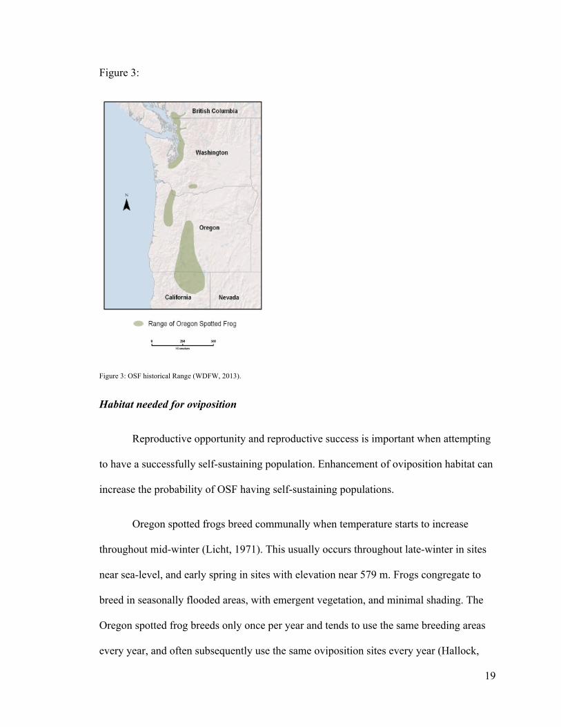
The OSF historically ranges from southwestern British Columbia, Canada to
northeastern California, USA (Figure 3) (Hallock, 2013). They are highly aquatic,
medium-sized frogs (McAllister & Leonard, 1997). The species has largely been
extirpated from its historical range, and current populations continue to be isolated and
diminished (Chelgren et al., 2008). It is estimated that approximately 78% of the OSF’s
historical range has been lost (McAllister & Leonard, 1997).
OSF’s breeding season is usually throughout late-winter or early spring. Females
lay egg masses in communal oviposition sites (i.e. in groups in direct contact), within
shallow areas, with slow moving water and low emergent vegetation. It takes from 18-30
days for eggs to hatch, then tadpoles develop for 13-16 weeks and undergo
metamorphosis throughout mid-summer. It takes OSF two or three years to mature and
start reproducing (McAllister & Leonard, 1997). OSF spends most of their life in aquatic
habitat, leaving occassionally only for short periods of time.
19
Figure 3:
Figure 3: OSF historical Range (WDFW, 2013).
Habitat needed for oviposition
Reproductive opportunity and reproductive success is important when attempting
to have a successfully self-sustaining population. Enhancement of oviposition habitat can
increase the probability of OSF having self-sustaining populations.
Oregon spotted frogs breed communally when temperature starts to increase
throughout mid-winter (Licht, 1971). This usually occurs throughout late-winter in sites
near sea-level, and early spring in sites with elevation near 579 m. Frogs congregate to
breed in seasonally flooded areas, with emergent vegetation, and minimal shading. The
Oregon spotted frog breeds only once per year and tends to use the same breeding areas
every year, and often subsequently use the same oviposition sites every year (Hallock,
20
2013). In years where hydrology is extreme (very low or very high waters), different sites
might be selected for oviposition. The OSF tends to move towards breeding sites
throughout the fall, when rain inundates the wetlands. Since the frog is highly aquatic,
periodically flooded wetlands become very important for the frog to reach oviposition
sites (Kapust et al., 2012; Hallock, 2013). The start of egg deposition depends on spring
conditions, and thus varies every year. OSF usually starts laying egg masses when
surface water temperatures reach 7-9°C. Once breeding starts, frogs usually lay their egg
masses communally over a short period of time. Moreover, the frog tends to lay their
eggs adjacent or on top of other egg masses (Hallock, 2013).
Pearl and colleagues found the mean water depth for oviposition to be 18.5 cm in
the state of Oregon, with occasional laying on top of floating vegetation mats (Pearl,
Adams, & Leuthold, 2009). This shows that emergent vegetation can be important for
OSF oviposition site selection, since it provides egg mass clusters with stability within
wetlands.
Effects of reed canary grass on Oregon spotted frog
There aren’t many studies on how RCG specifically influences the OSF, but given
observations, and known breeding habitat requirements, some inferences have been made
about the relationship between them. Kapust and colleagues (2012) conducted a study to
see if reduction of RCG height and density could improve oviposition habitat for the OSF
in Southwestern Washington. This study was done at West Rocky Prairie wildlife area.
The experiment consisted of monitoring 32 pairs of mowed and un-mowed plots, where
21
circular 30 m plots were mowed throughout the summer dry season using mechanical
weed-removal methods. The plots were specifically placed in areas where egg masses
had been observed in the year 2000. They found structural differences between mowed
and un-mowed plots were significant, since mowed plots showed little RCG growth.
They also found the median temperature difference to be 1.4°C (throughout oviposition
season) between mowed and un-mowed plots, with diurnal temperatures being
significantly higher in the mowed plots since decreasing RCG density exposes water to
direct sunlight (Kapust et al., 2012). Two clusters of egg masses were found in mowed
plots, and none in un-mowed ones. According to this study, mowing RCG throughout late
summer can provide OSF with desired habitat throughout oviposition time in the winter.
RCG infested wetlands can potentially be suitable OSF oviposition sites, if
density of the grass at oviposition time is suitable (Hallock, 2013). OSF requires habitat
that is shallow and seasonally flooded, and where emergent vegetation will not shade
eggs (Kapust et al., 2012), there is a variety of RCG control strategies that can be used to
serve this purpose. Additional studies are necessary to assess which treatment is most
efficient to reduce RCG densities in oviposition sites and provide OSF with desired
oviposition habitat.
Management strategies
Current management strategies for Oregon spotted frog in the state of Washington
involve mostly habitat enhancement, and control of non-native fish, wildife and
amphibian species to reduce predation (Hallock, 2013). The Washington Department of

22
Fish and Wildlife is currently trying to study and manage the existing Oregon spotted
frog by undertaking the following management activities: species monitoring, species
inventory, population reintroduction, protection and enhancement of significant habitat,
research to facilitate and enhance recovery, information management systems and
sharing, public information and education programs, and coordination and partnership
with several agencies (Hallock, 2013).
Specific management strategies in the state of Washington will depend on habitat
and population needs of specific populations. Continued population studies can provide
valuable information that can help specify management strategies needed in each of the
locations where OSF is currently found. The purpose of this study is to assess how
different RCG control treatments can influence important variables necessary for
successful OSF oviposition habitat (such as water depth, water temperatures, percentage
live RCG, percentage RCG thatch cover, percentage open water, emergent vegetation
height, RCG thatch height, dissolved oxygen concentrations, and conductivity levels)
between different wetlands.
23
CHAPTER 3: METHODS
This study was conducted based on the likelihood of covering the time span when
oviposition was bound to occur at these sites in Southern Washington. As such,
vegetation data, hydrological data, and chemical data were collected from February 6th
until March 13th, 2015. These dates of data collection were selected by analyzing surface
water temperatures continuously (given that once temperatures have passed the threshold
of 6°C, it is a trigger for oviposition) and studying past year’s oviposition timing for OSF
(White, 2002; Kapust et al., 2012). The dates included one week prior to oviposion, the
duration of oviposition period, and a week following oviposition period.
Study Areas
Two different sites were studied: West Rocky Prairie (WRP) and the Joint Base
Lewis-McChord (JBLM), with the purpose of comparing hydrologic, vegetation, and
chemical data between the sites in order to identify changes in wetland ecosystem
functions caused by RCG infestations. The study areas were selected because they are
infested with RCG, and work is being conducted related to OSF habitat enhancement.
OSF is present at both sites: naturally at WRP, and by translocation at JBLM. WRP is
considered a “successful site” within this study since RCG has been successfully treated
for OSF oviposition habitat (Kapust, 2012). JBLM is considered an “usuccessful site”
since most wetlands are RCG monocrops, and OSF oviposition has been unsuccessful at
this site so far.

24
The purpose of analyzing two different sites was to evaluate if any of the
treatments at JBLM (unsuccessful site), replicated successful OSF oviposition habitat
(WRP). In order to assess successful habitat, hydrologic (water depth, and water
temperature), vegetation (percentage live RCG, percentage RCG thatch height,
percentage open water, emergent vegetation height, and thatch height), and chemical
components (dissolved oxygen concentrations, and conductivity) were measured.
Joint Base Lewis-McChord (JBLM)
JBLM is located approximately 9 miles southwest of Tacoma, Washington,
U.S.A. Roughly 131 hectares of JBLM consist of wetlands that drain off of Muck Creek
(Richardson, 2011). These wetlands are connected seasonally via Muck Creek, and are
dominated by emergent vegetation such as cattail (Typha latifolia), reed canary grass
(Phalaris arundinacea), bulrush (Schoenoplectus acutus), pond shield (Potamogenton
spp), sedges (Carex spp), rushes (Juncus spp), and Eurasian watermilfoil (Myriophyllum
spicatum) (Richardson, 2011).
Three RCG-infested wetlands exist within this area (Johnson, ROTC Camp, and
Watkins Marsh) and all were originally selected for a RCG control pilot study. However,
upon inspection only two (Johnson and Watkins Marsh) (figure 4) were chosen for this
specific study since ROTC camp floods only every few years and therefore has lower
water levels year-round, which would not be suitable for OSF oviposition habitat.
There is no record of OSF ever existing naturally at JBLM. There currently is a
translocation program, where frogs are reared at Cedar Creek Correction Center by

25
inmate technicians, and later released within the wetlands at JBLM. The program started
in 2008 and approximately 500 frogs are released at JBLM every year (Hallock, 2013).
However, only one male OSF was observed this year near the Watkins plots.
Both sites contain five 10 x 10 meter plots (10 plots total for this study), each with
different treatments. Each of the sites (Johnson and Watkins) had 5 different treatments:
Mow/Burn/Herbicide (MBH), Mow/Burn (MB), Mow/Herbicide (MH), Burn/Herbicide
(BH), and a Control (C) treatment that was left as is (no treatment). Treatments have been
done once per year throughout late summer, starting in 2013. These treatments are part of
pilot study initiated by Sarah Hamman (CNLM).
For the treatments Aquamaster® Herbicide (aquatic approved glyphosate) was
used at 2% concentration with Liberate (non-ionic approved surfactant) to improve
herbicide performance. Herbicide was applied at different times of the year, depending on
the treatments: Mow/Burn/Herbicide was mowed in late June/early July (before seed
heads fully formed), sprayed in early August, and burned in early September. The
Burn/Herbicide treatment was sprayed in early August, and burned in early September.
The Mow/Herbicide treatment was mowed in June/early July, and sprayed in
September/October. And finally the Mow/Burn treatment was mowed in late July, and
burned in early September. Backing burns were used to move fire through the plots
slowly in order to consume as much litter and duff as possible, and brushcutting was used
to cut down the standings clumps before the seed heads were fully formed each year.
26
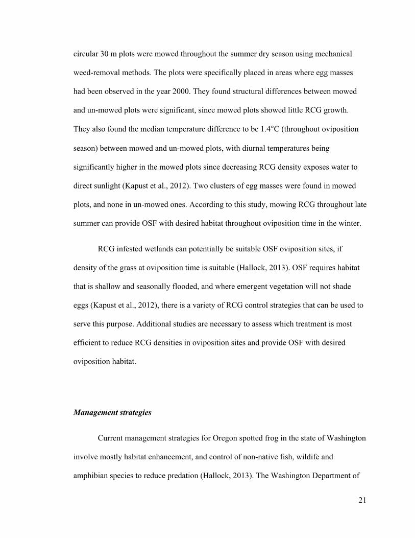
Figure 4:
Figure 4: Location of Watkins and Johnson sites within Joint Base Lewis-McChord, with the corresponding positioning of treatment plots (MBH representing Mow/Burn/Herbicide treatment, MB respresenting Mow/Burn treatment, MH representing Mow/Herbicide treatment, BH representing Burn/Herbicide, and C representing the Control treatment.
West Rocky Prairie
The West Rocky Prairie Wildlife Area is a 324-ha wetland complex located
northwest of Tenino, in Thurston County, U.S.A., and it is currently managed by the
Washington Department of Fish and Wildlife (Kapust, 2012). This study site was
historically agricultural land, and was actively cultivated until mid-1980’s (Kapust,
2012). Since then, the Washington Department of Fish and Wildlife has designated WRP
as a wildlife area, and has allowed for historical prairie conditions to resurface in the
area.
Johnson
Watkins

27
WRP is a historical site for OSF. Two units within this area are currently occupied
by Rana pretiosa, one of them at the headwaters of Allen Creek (hereafter West area),
and another one in a small tributary of Beaver Creek (hereafter East area) (Figure 5). This
study was specifically conducted on the West area, since it is where most of the OSF
oviposition activity happens. The West Area consists of 12 ha dominated by RCG, but
Slough and Beaked sedges (Carex obnupta, C. utriculata) can also be found (Tyson &
Hayes, 2014).
The West Area contains eight 15 x 30 m plots total: four treated (T1, T2, T3, and
T4), and four control plots (C1, C2, C3 and C4) (Figure 6). The treatment consisted of
mowing RCG once per year throughout the summer. For this study, data was taken only
from the mowed plots, since it is where most OSF oviposition activity takes place (only
two egg masses found outside treated plots in 2010, and areas had similar characteristics
as mowed plots). This site is critical, since over 145 egg masses were found between
2009 and 2011, and number of egg masses have been increasing since treatments started.
As such, by studying water characteristics, vegetation cover, and chemical characteristics
of the successful site, it will be possible to infer which characteristics are more ideal for
OSF oviposition.
28
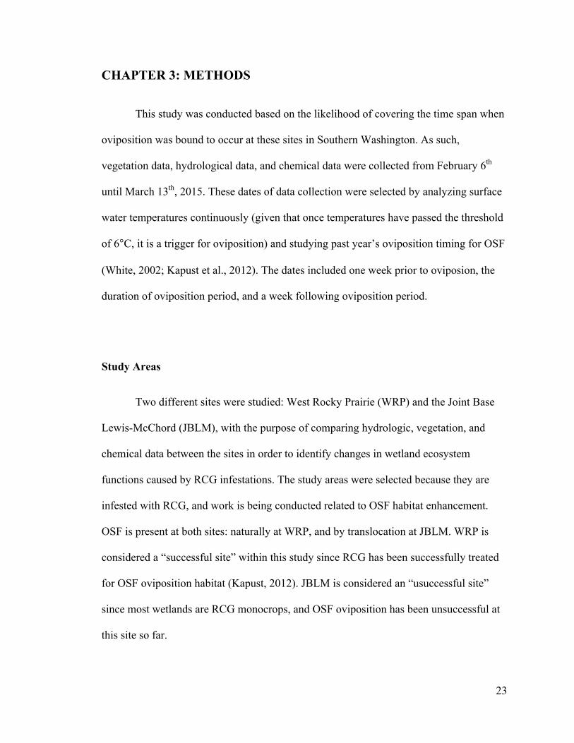
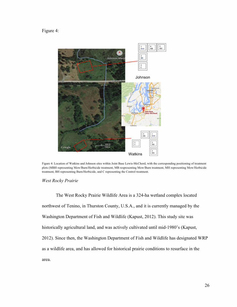
Figure 5:
Figure 5: Location of West Rocky Prairie in Western Washington, with headwaters Allen Creek (West Side), and Beaver Creek (East Side). Red boxes indicate location of West and East Areas (Tyson & Hayes, 2014).
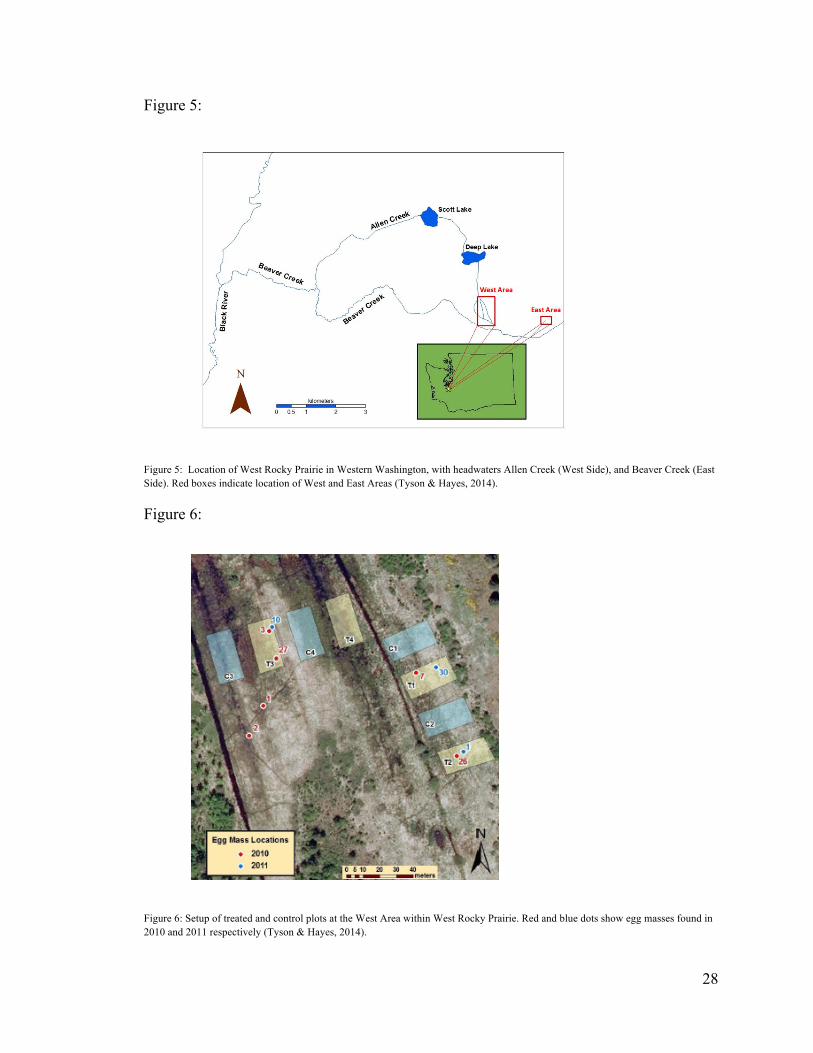
Figure 6:
Figure 6: Setup of treated and control plots at the West Area within West Rocky Prairie. Red and blue dots show egg masses found in 2010 and 2011 respectively (Tyson & Hayes, 2014).

29
Field Survey Methods: Vegetation Data
Vegetation conditions are important for determining suitable OSF ovipositon
habitat. OSF prefers sites with emergent or floating vegetation, and open water habitat
(McAllister & Leonard, 1997). Vegetation analysis consisted of measuring percent cover
to estimate ground cover of live RCG, RCG thatch cover, open water (or bare ground)
within each plot, as well as RCG thatch height and emergent vegetation height at both
sites. Vegetation analysis was conducted once at the beginning of the study (February
10th, 2015) and once at the end of the study (March 13th, 2015).
JBLM
There were a total of 10 plots: 5 at Johnson, and 5 at Watkins. Every 10 x 10 m
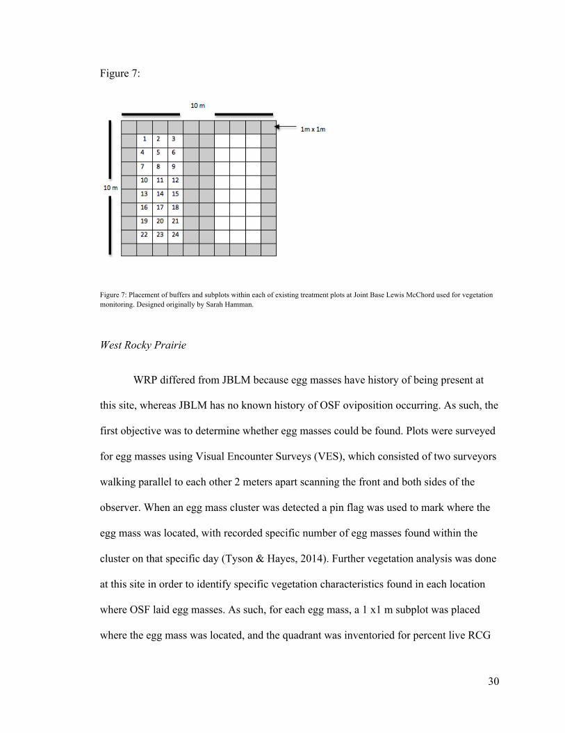
plot was analyzed by randomly assigning 1 X 1 m subplots within each 10 x 10 m plot
using a random number generator to place the subplot in 1 of 24 possible locations
(Figure 7). A 1 m buffer area within the perimeter of each 10 x 10 m plot was excluded in
order to buffer against external influential factors. Three subplots were assessed within
each of the plots to account for variation.
Each 1 X 1 meter subplot was inventoried for: percent RCG cover, percent thatch
cover, percent bare ground/open water, and percent cover of other species. In order to
assess vertical vegetation structure each 1 x 1 meter subplot was inventoried for both
thatch height and emergent vegetation height (in cm) (as depicted in the section titled
“Vegetation Monitoring”).
30
Figure 7:
Figure 7: Placement of buffers and subplots within each of existing treatment plots at Joint Base Lewis McChord used for vegetation monitoring. Designed originally by Sarah Hamman.
West Rocky Prairie
WRP differed from JBLM because egg masses have history of being present at
this site, whereas JBLM has no known history of OSF oviposition occurring. As such, the
first objective was to determine whether egg masses could be found. Plots were surveyed
for egg masses using Visual Encounter Surveys (VES), which consisted of two surveyors
walking parallel to each other 2 meters apart scanning the front and both sides of the
observer. When an egg mass cluster was detected a pin flag was used to mark where the
egg mass was located, with recorded specific number of egg masses found within the
cluster on that specific day (Tyson & Hayes, 2014). Further vegetation analysis was done
at this site in order to identify specific vegetation characteristics found in each location
where OSF laid egg masses. As such, for each egg mass, a 1 x1 m subplot was placed
where the egg mass was located, and the quadrant was inventoried for percent live RCG

31
cover, percent RCG thatch cover, percent open water, emergent vegetation height, and
thatch height.
Additionally, for general plot conditions every plot was analyzed by randomly
assigning two numbers (one for vertical length from 1 to 30, and one for horizontal length
from 1 to 15) and then measuring them out with a meter to place a 1 x 1 meter subplot
within each 15 x 30 meter plot. Three subplots were assessed for each plot to account for
variation in vegetation parameters (depicted in the section below “Vegetation
Monitoring”).
Vegetation Monitoring
At both JBLM and WRP each 1 X 1 meter subplot was inventoried for percent
live RCG cover, percent RCG thatch cover, and percent open water. In order to assess
vertical vegetation structure each 1 x 1 meter subplot was inventoried for both RCG
thatch height and emergent vegetation height (in cm).
Percentage RCG cover was calculated by placing a 1 x 1 meter quadrant frame,
and visually calculating the percentage. Percent thatch cover (which included floating
thatch visually in contact with surface water) was calculated in the same manner, as well
as percent bare ground/open water, and percent cover of other species.
Vertical vegetation structure was measured by examining thatch height by
applying pressure and inserting a PVC pipe (with marked measured centimeters) to the
bottom of the wetland and marking the exact spot where RCG thatch was the highest (In

32
order to measure thickness of submerged thatch). Emergent vegetation was measured by
using the same marked PVC pipe and measuring the highest point of emergent vegetation
from the surface water.
Field Survey Methods: Chemical and Hydrological Data
Chemical data collection consisted of measuring dissolved oxygen (mg/L),
percentage dissolved oxygen (%DO/L), conductivity (µS/cm), temperature (°C) and
salinity (ppt) using a YSI model YSI Pro2030 (cable model 6052030 Pro Series
DO/Conductivity Cable). The data was taken on the following dates:
-‐ West Rocky Prairie: February 10th, February 13th, February 17th, February 20th,
February 24th, February 27th, March 3rd, March 6th, March 11th,
-‐ JBLM: February 13th, February 20th, February 27th, March 12th
Dissolved oxygen, conductivity, temperature, and salinity were taken by submerging
the tip of the probe until it was completely submerged but not touching the bottom of the
wetland or any other floating or emergent vegetation. Measurements were taken once on
each plot, without replication for both JBLM and WRP on dates mentioned above. On
WRP each measurement was taken on the most southeastern corner of each plot, and on
JBLM each measurement was taken next to data logger setup. Time was recorded with
each measurement.
Additional hydrological data was taken in both sites with the use of dataloggers
(HOBO U20L). The data loggers measured water temperature and height of surface water
every 30 minutes continuously throughout oviposition time, and data was downloaded
33
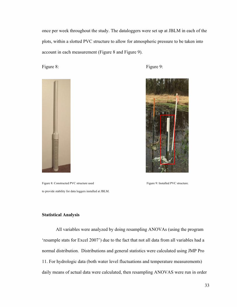
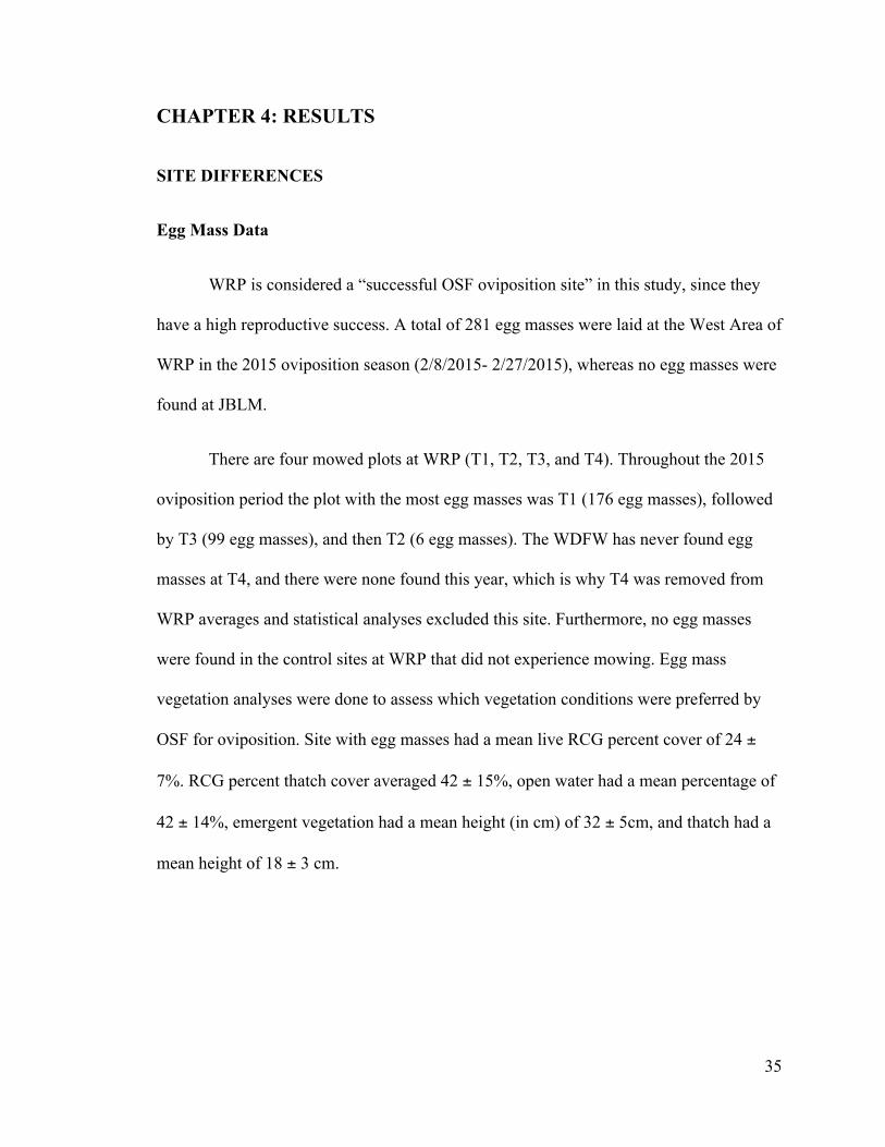
once per week throughout the study. The dataloggers were set up at JBLM in each of the
plots, within a slotted PVC structure to allow for atmospheric pressure to be taken into
account in each measurement (Figure 8 and Figure 9).
Figure 8: Figure 9:
Figure 8: Constructed PVC structure used Figure 9: Installed PVC structure.
to provide stability for data loggers installed at JBLM.
Statistical Analysis
All variables were analyzed by doing resampling ANOVAs (using the program
‘resample stats for Excel 2007’) due to the fact that not all data from all variables had a
normal distribution. Distributions and general statistics were calculated using JMP Pro
11. For hydrologic data (both water level fluctuations and temperature measurements)
daily means of actual data were calculated, then resampling ANOVAS were run in order

34
to see how different treatments affected water depth and temperature fluctuations over
oviposition time. Additional resampling ANOVAS were done in order to see how
hydrologic components differed between Johnson and Watkins.
Vegetation data (% live RCG, % RCG thatch cover, % open water, RCG thatch
height, and emergent vegetation height) was analyzed also by running resampling
ANOVAs in order to compare differences between sites and also between treatments.
The same was done for abiotic data (dissolved oxygen and conductivity). The original
data collected was used to run ANOVAs, which were done to compare the means of each
of the vegetation variables between the different treatments using resampling stats for
Excel.
Moreover, for all variables (within JBLM plots) further analysis was done to
compare each of the treatments (MBH, MB, MH, and BH) to the control treatment (C).
Resampling ANOVAs were run between each treatment and their corresponding control
plot (for both Watkins and Johnson).
35
CHAPTER 4: RESULTS
SITE DIFFERENCES
Egg Mass Data
WRP is considered a “successful OSF oviposition site” in this study, since they
have a high reproductive success. A total of 281 egg masses were laid at the West Area of
WRP in the 2015 oviposition season (2/8/2015- 2/27/2015), whereas no egg masses were
found at JBLM.
There are four mowed plots at WRP (T1, T2, T3, and T4). Throughout the 2015
oviposition period the plot with the most egg masses was T1 (176 egg masses), followed
by T3 (99 egg masses), and then T2 (6 egg masses). The WDFW has never found egg
masses at T4, and there were none found this year, which is why T4 was removed from
WRP averages and statistical analyses excluded this site. Furthermore, no egg masses
were found in the control sites at WRP that did not experience mowing. Egg mass
vegetation analyses were done to assess which vegetation conditions were preferred by
OSF for oviposition. Site with egg masses had a mean live RCG percent cover of 24 ±
7%. RCG percent thatch cover averaged 42 ± 15%, open water had a mean percentage of
42 ± 14%, emergent vegetation had a mean height (in cm) of 32 ± 5cm, and thatch had a
mean height of 18 ± 3 cm.
36
Chemical Data
Chemical data was analyzed between sites to assess if there were any significant
differences between “successful” and “unsuccessful” sites (when it comes to dissolved
oxygen concentrations and conductivity) that could attribute to the reasons why egg
masses were found only at one of these locations (WRP).
Conductivity
Conductivity is important when it comes to amphibians, since they tend to be
fairly sensitive species and have low tolerance levels, which can in turn affect occupancy
of potential breeding sites(Klaver, Peterson, & Patla, 2013). Total site conductivity
ranged from 69.1- 94.9, 68.7-104.6, and 19.5-103 µS/cm for Watkins, Johnson, and WRP
respectively (Mean= 84.5, Std. Dev.= 7.4; Mean= 89.7, Std. Dev.= 12.5; and Mean=
61.2, Std. Dev.= 18.9488; respectively). The average conductivity analysis shows the plot
with the lowest conductivity at JBLM is the Control treatment at the Johnson site,
ranging from 68.7-81.5 µS/cm (Mean= 73.1 µS/cm , Std. Dev.= 5.8).
Looking at the differences in average SPC between WRP (“successful site”) and
JBLM sites (“unsuccessful sites”), most sites at JBLM have much higher SPC than what
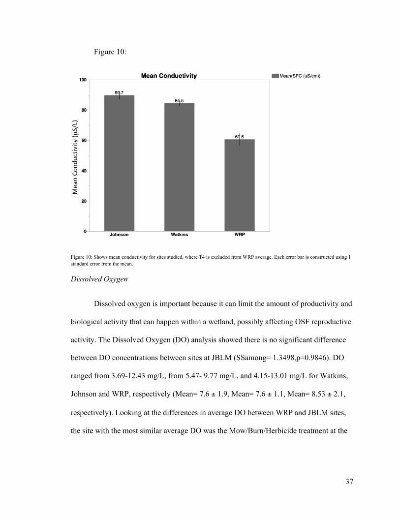
is found at WRP (Figure 10). Data analysis showed there was no significant difference in
conductivity between treatments for both Watkins and Johnson (SSamong= 773.126, p=
0.126).
37
Figure 10:
Figure 10: Shows mean conductivity for sites studied, where T4 is excluded from WRP average. Each error bar is constructed using 1 standard error from the mean.
Dissolved Oxygen
Dissolved oxygen is important because it can limit the amount of productivity and
biological activity that can happen within a wetland, possibly affecting OSF reproductive
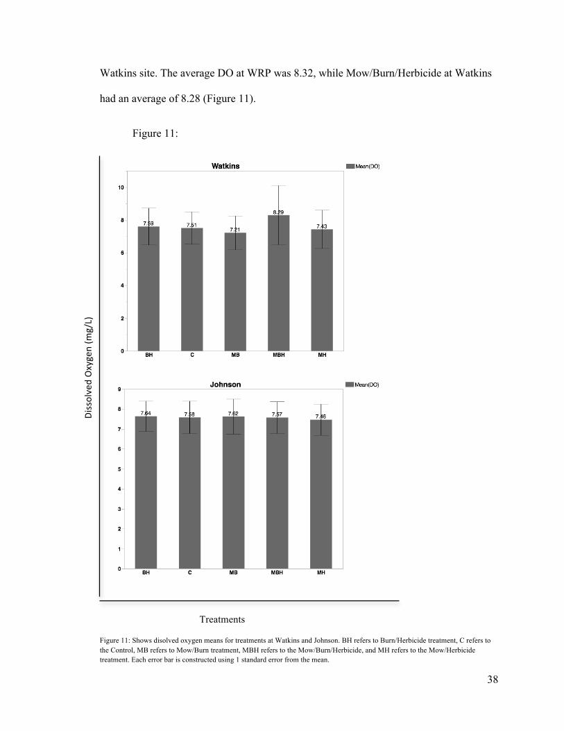
activity. The Dissolved Oxygen (DO) analysis showed there is no significant difference
between DO concentrations between sites at JBLM (SSamong= 1.3498,p=0.9846). DO
ranged from 3.69-12.43 mg/L, from 5.47- 9.77 mg/L, and 4.15-13.01 mg/L for Watkins,
Johnson and WRP, respectively (Mean= 7.6 ± 1.9, Mean= 7.6 ± 1.1, Mean= 8.53 ± 2.1,
respectively). Looking at the differences in average DO between WRP and JBLM sites,
the site with the most similar average DO was the Mow/Burn/Herbicide treatment at the
Mean Co
nductivity (µ
S/L)
38
Watkins site. The average DO at WRP was 8.32, while Mow/Burn/Herbicide at Watkins
had an average of 8.28 (Figure 11).
Figure 11:
Treatments
Figure 11: Shows disolved oxygen means for treatments at Watkins and Johnson. BH refers to Burn/Herbicide treatment, C refers to the Control, MB refers to Mow/Burn treatment, MBH refers to the Mow/Burn/Herbicide, and MH refers to the Mow/Herbicide treatment. Each error bar is constructed using 1 standard error from the mean.
Dissolved
Oxygen (m
g/L)
39
Hydrologic Data:
Temperature
Temperature is one of the most important factors when it comes to OSF
oviposition, it has been used to determine when and if OSF is able to start laying egg
masses (once temperatures reach 6°C). Low temperatures can lead to egg mass mortality,
which is why temperature stability is important throughout OSF oviposition period.
Results show temperature differences between WRP and JBLM. Temperatures in WRP
range from 6.1-9.8 °C, from 5.3 - 13.4 °C at Johnson, and from 5.5 - 10.8°C at Watkins.
There was a higher range in variability of temperature at the two sites in JBLM,
indicating less temperature stability.
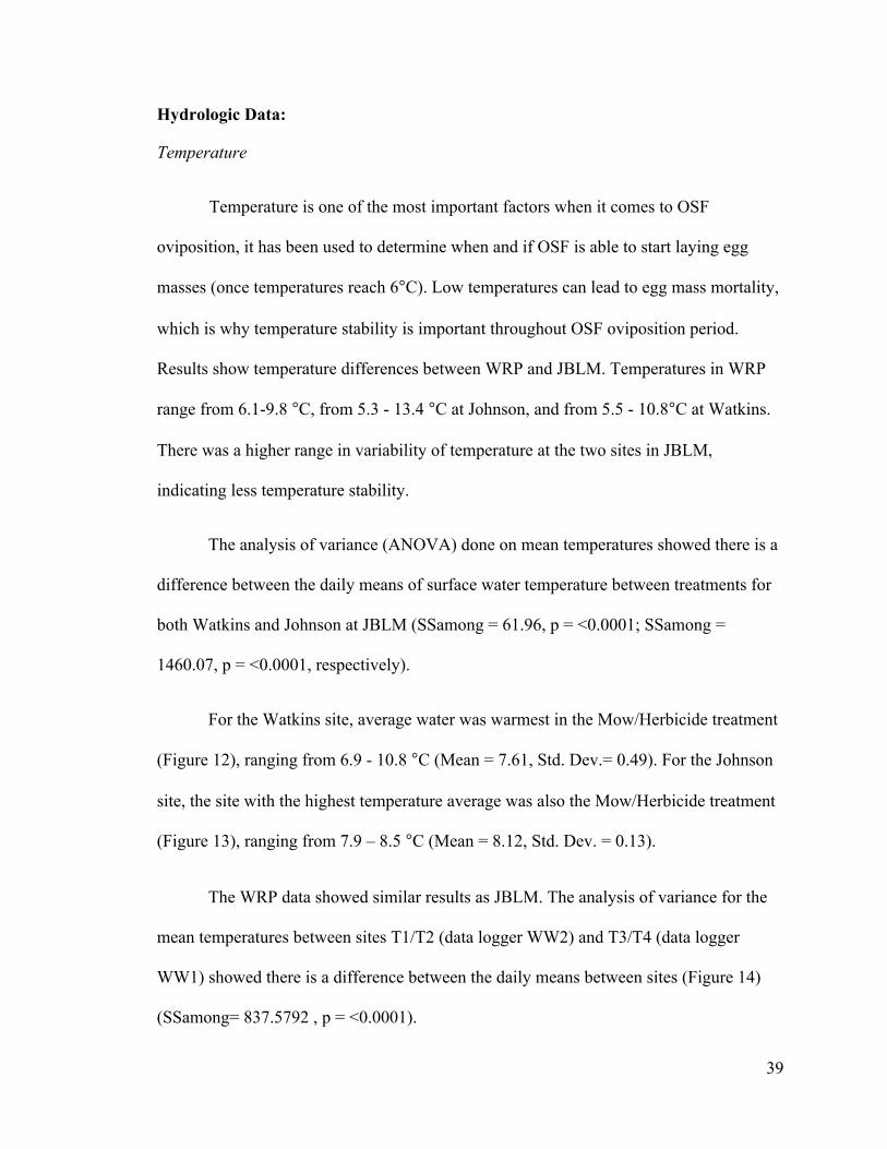
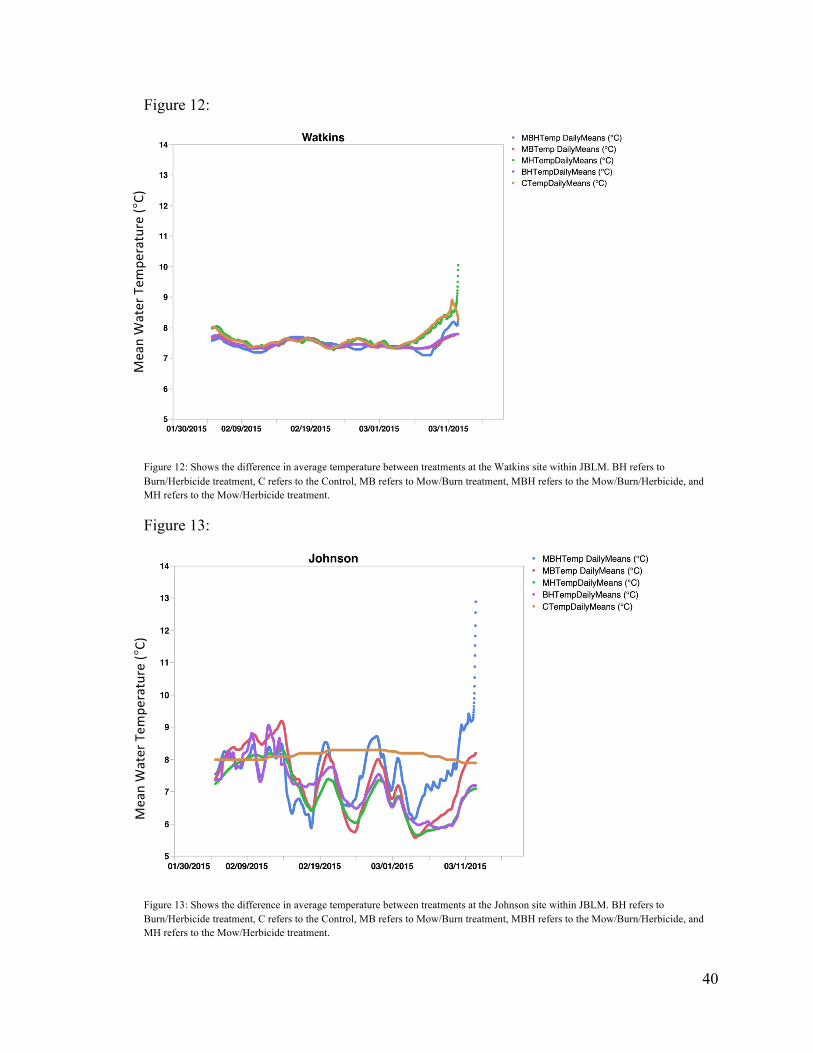
The analysis of variance (ANOVA) done on mean temperatures showed there is a
difference between the daily means of surface water temperature between treatments for
both Watkins and Johnson at JBLM (SSamong = 61.96, p = <0.0001; SSamong =
1460.07, p = <0.0001, respectively).
For the Watkins site, average water was warmest in the Mow/Herbicide treatment
(Figure 12), ranging from 6.9 - 10.8 °C (Mean = 7.61, Std. Dev.= 0.49). For the Johnson
site, the site with the highest temperature average was also the Mow/Herbicide treatment
(Figure 13), ranging from 7.9 – 8.5 °C (Mean = 8.12, Std. Dev. = 0.13).
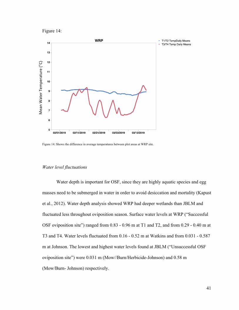
The WRP data showed similar results as JBLM. The analysis of variance for the
mean temperatures between sites T1/T2 (data logger WW2) and T3/T4 (data logger
WW1) showed there is a difference between the daily means between sites (Figure 14)
(SSamong= 837.5792 , p = <0.0001).
40
Figure 12:
Figure 12: Shows the difference in average temperature between treatments at the Watkins site within JBLM. BH refers to Burn/Herbicide treatment, C refers to the Control, MB refers to Mow/Burn treatment, MBH refers to the Mow/Burn/Herbicide, and MH refers to the Mow/Herbicide treatment.
Figure 13:
Figure 13: Shows the difference in average temperature between treatments at the Johnson site within JBLM. BH refers to Burn/Herbicide treatment, C refers to the Control, MB refers to Mow/Burn treatment, MBH refers to the Mow/Burn/Herbicide, and MH refers to the Mow/Herbicide treatment.
Mean Water Tem
perature (°C)
Mean Water Tem
perature (°C)
41
Figure 14:
Figure 14: Shows the difference in average temperatures between plot areas at WRP site.
Water level fluctuations
Water depth is important for OSF, since they are highly aquatic species and egg
masses need to be submerged in water in order to avoid desiccation and mortality (Kapust
et al., 2012). Water depth analysis showed WRP had deeper wetlands than JBLM and
fluctuated less throughout oviposition season. Surface water levels at WRP (“Successful
OSF oviposition site”) ranged from 0.83 - 0.96 m at T1 and T2, and from 0.29 - 0.40 m at
T3 and T4. Water levels fluctuated from 0.16 - 0.52 m at Watkins and from 0.031 - 0.587
m at Johnson. The lowest and highest water levels found at JBLM (“Unsuccessful OSF
oviposition site”) were 0.031 m (Mow//Burn/Herbicide-Johnson) and 0.58 m
(Mow/Burn- Johnson) respectively.
Mean Water Tem
perature (°C)

42
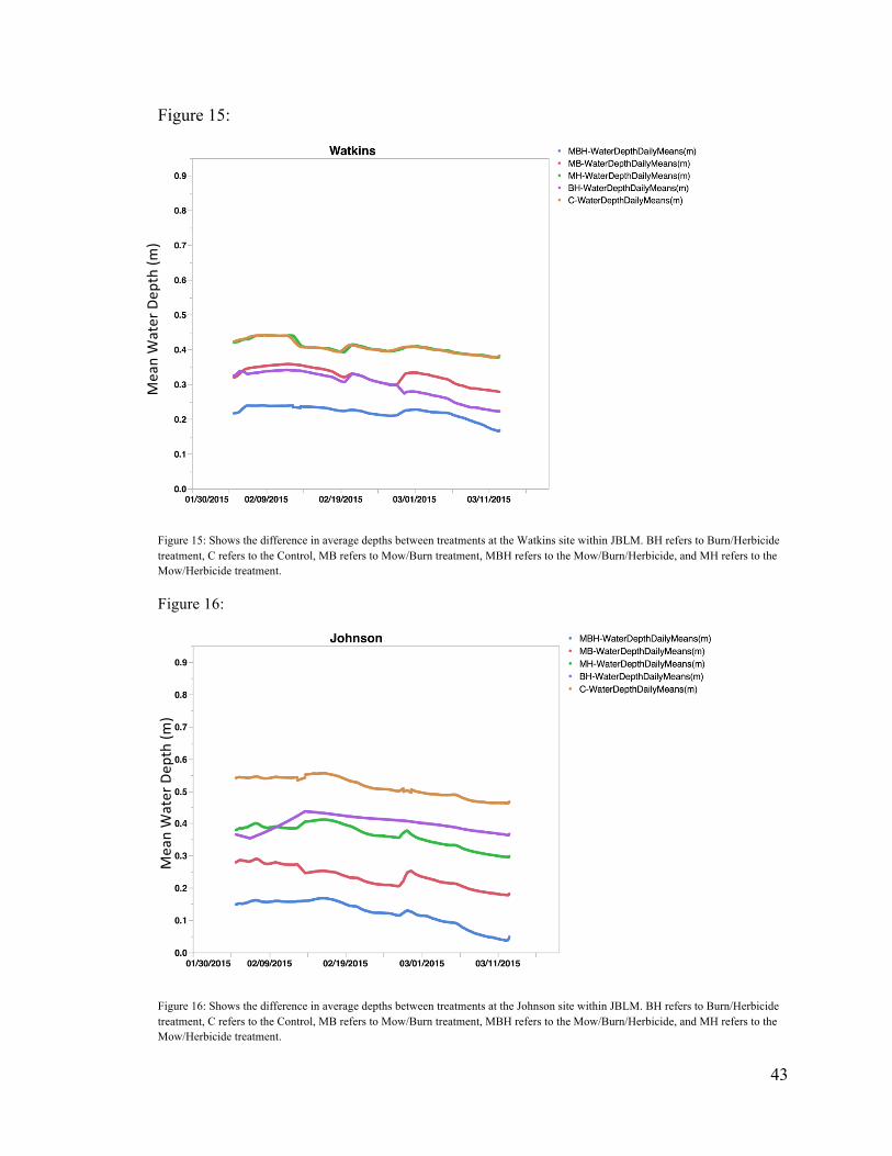
The analysis of variance (ANOVA) done on mean depths for JBLM showed there
is a difference between the daily means water depths between treatments for both
Watkins and Johnson (SSamong = 43.06, p = <0.0001; SSamong = 157.68, p = <0.0001,
respectively).
For the Watkins site, average water was highest in the Mow/Herbicide treatment
(Figure 15), ranging from 0.37 - 0.44 m (Mean = 0.41, Std. Dev.= 0.02). For the Johnson
site, the site with the highest water depth average was the control treatment (Figure 16),
ranging from 0.29 - 0.42 m (Mean = 0.37, Std. Dev. = 0.03).
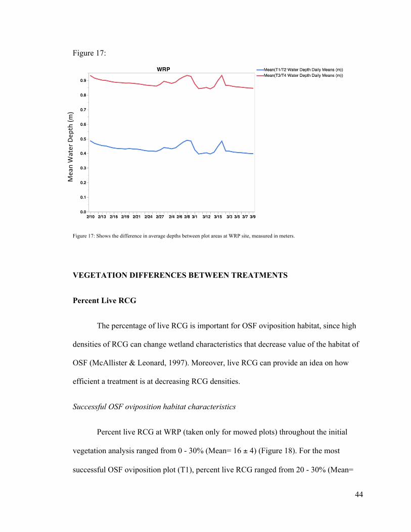
The WRP data showed similar results as JBLM. The analysis of variance for the
mean depths between sites T1/T2 (data logger WW2) and T3/T4 (data logger WW1)
showed there is a difference between the daily means between sites (Figure 17)
(SSamong= 103.81, p = <0.0001).
43
Figure 15:
Figure 15: Shows the difference in average depths between treatments at the Watkins site within JBLM. BH refers to Burn/Herbicide treatment, C refers to the Control, MB refers to Mow/Burn treatment, MBH refers to the Mow/Burn/Herbicide, and MH refers to the Mow/Herbicide treatment.
Figure 16:
Figure 16: Shows the difference in average depths between treatments at the Johnson site within JBLM. BH refers to Burn/Herbicide treatment, C refers to the Control, MB refers to Mow/Burn treatment, MBH refers to the Mow/Burn/Herbicide, and MH refers to the Mow/Herbicide treatment.
Mean Water Dep
th (m
) Mean Water Dep
th (m
)
44
Figure 17:
Figure 17: Shows the difference in average depths between plot areas at WRP site, measured in meters.
VEGETATION DIFFERENCES BETWEEN TREATMENTS
Percent Live RCG
The percentage of live RCG is important for OSF oviposition habitat, since high
densities of RCG can change wetland characteristics that decrease value of the habitat of
OSF (McAllister & Leonard, 1997). Moreover, live RCG can provide an idea on how
efficient a treatment is at decreasing RCG densities.
Successful OSF oviposition habitat characteristics
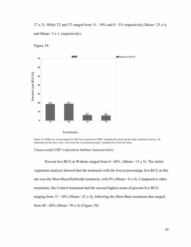
Percent live RCG at WRP (taken only for mowed plots) throughout the initial
vegetation analysis ranged from 0 - 30% (Mean= 16 ± 4) (Figure 18). For the most
successful OSF oviposition plot (T1), percent live RCG ranged from 20 - 30% (Mean=
Mean Water Dep
th (m
) Mean Water Dep
th (m
)
45
27 ± 3). While T2 and T3 ranged from 15 - 30% and 0 - 5% respectively (Mean= 23 ± 4,
and Mean= 3 ± 1, respectively).
Figure 18:
Treatments
Figure 18: Difference of percentage live RCG per treatment in WRP, including the initial and the final vegetation analysis. All treatments are the same: mow. Each error bar is constructed using 1 standard error from the mean.
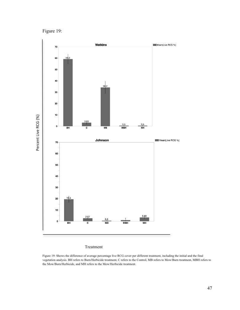
Unsuccessful OSF oviposition habitat characteristics
Percent live RCG at Watkins ranged from 0 - 60% (Mean= 15 ± 5). The initial
vegetation analysis showed that the treatment with the lowest percentage live RCG at this
site was the Mow/Burn/Herbicide treatment, with 0% (Mean= 0 ± 0). Compared to other
treatments, the Control treatment had the second highest mean of percent live RCG
ranging from 15 - 30% (Mean= 22 ± 4), following the Mow/Burn treatment that ranged
from 40 - 60% (Mean= 50 ± 6) (Figure 19).
Percen
t Live RC
G (%
)

46
Percent live RCG at Johnson ranged from 0 - 17% (Mean = 3.7 ± 1.6). The
treatment with the lowest mean percentage live RCG was the Control plot with 0% live
RCG, due to excessive thatch (Mean= 0 ± 0). Compared to the Control treatment, all
treatments had higher percentages of live RCG, with the highest one being the Mow/Burn
treatment ranging from 15 -17% (Mean 16 ± 1) (Figure 19).
Data analysis showed there is a significant difference between Johnson and
Watkins (SSamong= 997.63, p=0.044) when it comes to percentage live RCG. Additional
analysis showed there was also a significant difference in percent live RCG between the
different treatments for both Watkins and Johnson (SSamong= 4532.3, p=0.0002). When
comparing each of the treatments to the controls, the only plot with significant difference
between means for percentage live RCG was the Mow/Burn treatment (SSamong= 1452,
p=0.0408) for both Johnson and Watkins.
Looking at the conditions where OSF has been successful, the treatment that had
similar percent live RCG to those at WRP was the Control treatment at Watkins (Table
1). No treatments at Johnson were found within the successful OSF oviposition range as
seen in WRP (Table 2).
47
Figure 19:
Treatment
Figure 19: Shows the difference of average percentage live RCG cover per different treatment, including the initial and the final vegetation analysis. BH refers to Burn/Herbicide treatment, C refers to the Control, MB refers to Mow/Burn treatment, MBH refers to the Mow/Burn/Herbicide, and MH refers to the Mow/Herbicide treatment.
Percen
t Live RC
G (%
)

48
Percent RCG Thatch Cover
Percent thatch cover can be useful for OSF throughout oviposition time, since it
can provide egg masses with stability, and OSF tends to prefers sites where emergent or
floating vegetation is available (McAllister & Leonard, 1997). However, excess of thatch
can lead alterations to wetland hydrology (reducing water level), which can lead to
undesired conditions for OSF.
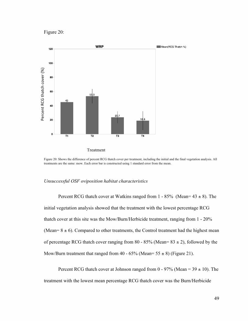
Successful OSF oviposition habitat characteristics
Percentage thatch cover at WRP throughout the initial vegetation analysis ranged
from 5-95% (Mean= 49 ± 9) (Figure 20). For the most successful OSF oviposition plot
(T1), percentage RCG thatch cover ranged from 60 - 75% (Mean= 68 ± 5). While T2 and
T3 ranged from 40-95% and 5 - 35% respectively (Mean= 62 ± 17, and Mean= 17 ± 9,
respectively).
49
Figure 20:
Treatment
Figure 20: Shows the difference of percent RCG thatch cover per treatment, including the initial and the final vegetation analysis. All treatments are the same: mow. Each error bar is constructed using 1 standard error from the mean.
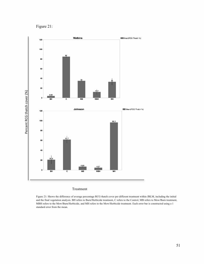
Unsuccessful OSF oviposition habitat characteristics
Percent RCG thatch cover at Watkins ranged from 1 - 85% (Mean= 43 ± 8). The
initial vegetation analysis showed that the treatment with the lowest percentage RCG
thatch cover at this site was the Mow/Burn/Herbicide treatment, ranging from 1 - 20%
(Mean= 8 ± 6). Compared to other treatments, the Control treatment had the highest mean
of percentage RCG thatch cover ranging from 80 - 85% (Mean= 83 ± 2), followed by the
Mow/Burn treatment that ranged from 40 - 65% (Mean= 55 ± 8) (Figure 21).
Percent RCG thatch cover at Johnson ranged from 0 - 97% (Mean = 39 ± 10). The
treatment with the lowest mean percentage RCG thatch cover was the Burn/Herbicide
Percen
t RCG
thatch cover (%
)

50
plot ranging from 0 - 10% (Mean= 5 ± 3). Compared to the Control treatment, which
ranged from 95 - 97% (Mean= 96 ± 0.7), all treatments had lower percentages of RCG
thatch cover, with the second highest one being the Mow/Herbicide treatment ranging
from 50-85% (Mean 67 ± 10) (Figure 21).
The resampling ANOVA showed that there was no significant difference between
the two sites (Johnson and Watkins) when it comes to percentage RCG thatch cover
(SSamong= 136.53, p=0.7317). Additional analysis showed percent RCG thatch cover
differed between treatments for both Watkins and Johnson (SSamong= 28692.9,
p<0.0001). When comparing each treatment to the control plots, all treatments showed
significant difference between the means for percentage RCG thatch cover relative to the
control (SSamong= 18330.08, p< 0.0001 for MBH; SSamong= 8374.08, p,0.0001 for
MB; SSamong= 2760.33, p= 0.009 for MH; and SSamong= 20750.08, p< 0.0001 for
BH) for both Watkins and Johnson.
Looking at the conditions where OSF has been successful, the treatments that had
similar percentage of RCG thatch cover averages to those at WRP were the Mow/Burn,
and Mow/Herbicide treatments at Watkins (Table 1), and the Mow/Herbicide treatment at
Johnson (Table 2).
51
Figure 21:
Treatment
Figure 21: Shows the difference of average percentage RCG thatch cover per different treatment within JBLM, including the initial and the final vegetation analysis. BH refers to Burn/Herbicide treatment, C refers to the Control, MB refers to Mow/Burn treatment, MBH refers to the Mow/Burn/Herbicide, and MH refers to the Mow/Herbicide treatment. Each error bar is constructed using a 1 standard error from the mean.
Percen
t RCG
thatch cover (%
)
52
Percent Open Water
The OSF is a highly aquatic species (McAllister & Leonard, 1997). Open water
habitat is important throughout oviposition season in order for OSF to move from
breeding site to breeding site. It is especially important throughout low water periods,
since it can provide egg masses with water necessary to avoid desiccation and ensure
reproductive success.
Successful OSF oviposition habitat characteristics
Percentage open water at WRP throughout the initial vegetation analysis ranged
from 1 - 80% (Mean= 36 ± 9) (Figure 22). For the most successful OSF oviposition plot
(T1), percentage open water ranged from 7 - 35% (Mean= 17 ± 9). While T2 and T3
ranged from 1 - 55% and 27 -80% respectively (Mean= 28 ± 16, and Mean= 57 ± 16,
respectively).
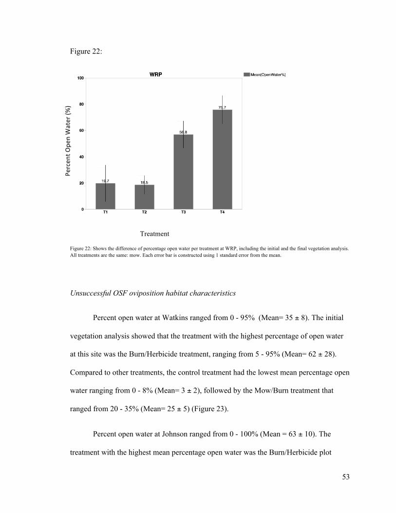
53
Figure 22:
Treatment
Figure 22: Shows the difference of percentage open water per treatment at WRP, including the initial and the final vegetation analysis. All treatments are the same: mow. Each error bar is constructed using 1 standard error from the mean.
Unsuccessful OSF oviposition habitat characteristics
Percent open water at Watkins ranged from 0 - 95% (Mean= 35 ± 8). The initial
vegetation analysis showed that the treatment with the highest percentage of open water
at this site was the Burn/Herbicide treatment, ranging from 5 - 95% (Mean= 62 ± 28).
Compared to other treatments, the control treatment had the lowest mean percentage open
water ranging from 0 - 8% (Mean= 3 ± 2), followed by the Mow/Burn treatment that
ranged from 20 - 35% (Mean= 25 ± 5) (Figure 23).
Percent open water at Johnson ranged from 0 - 100% (Mean = 63 ± 10). The
treatment with the highest mean percentage open water was the Burn/Herbicide plot
Percen
t Ope
n Water (%
)
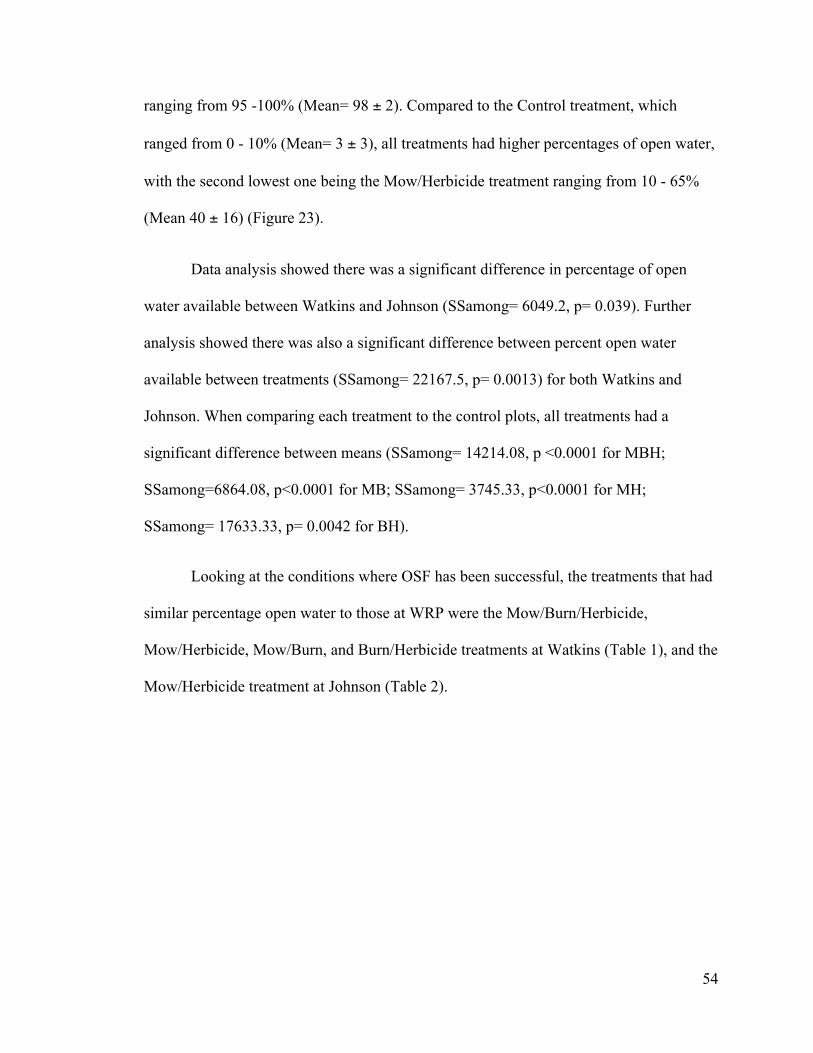
54
ranging from 95 -100% (Mean= 98 ± 2). Compared to the Control treatment, which
ranged from 0 - 10% (Mean= 3 ± 3), all treatments had higher percentages of open water,
with the second lowest one being the Mow/Herbicide treatment ranging from 10 - 65%
(Mean 40 ± 16) (Figure 23).
Data analysis showed there was a significant difference in percentage of open
water available between Watkins and Johnson (SSamong= 6049.2, p= 0.039). Further
analysis showed there was also a significant difference between percent open water
available between treatments (SSamong= 22167.5, p= 0.0013) for both Watkins and
Johnson. When comparing each treatment to the control plots, all treatments had a
significant difference between means (SSamong= 14214.08, p <0.0001 for MBH;
SSamong=6864.08, p<0.0001 for MB; SSamong= 3745.33, p<0.0001 for MH;
SSamong= 17633.33, p= 0.0042 for BH).
Looking at the conditions where OSF has been successful, the treatments that had
similar percentage open water to those at WRP were the Mow/Burn/Herbicide,
Mow/Herbicide, Mow/Burn, and Burn/Herbicide treatments at Watkins (Table 1), and the
Mow/Herbicide treatment at Johnson (Table 2).
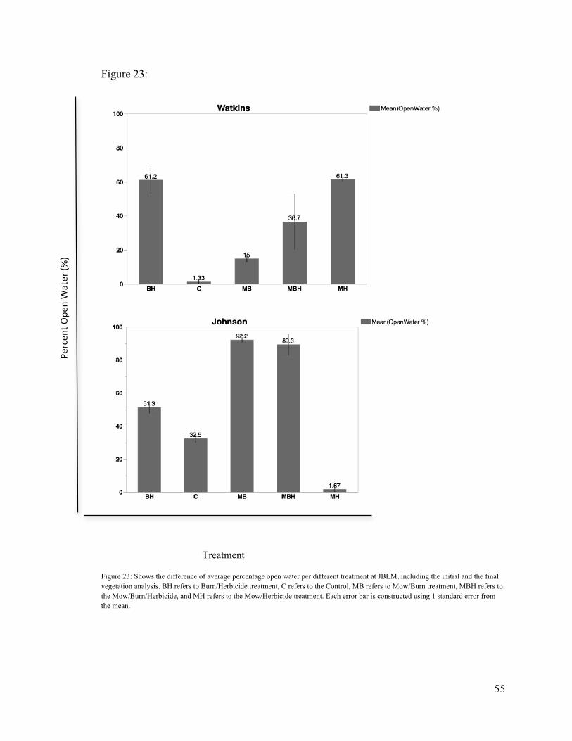
55
Figure 23:
Treatment
Figure 23: Shows the difference of average percentage open water per different treatment at JBLM, including the initial and the final vegetation analysis. BH refers to Burn/Herbicide treatment, C refers to the Control, MB refers to Mow/Burn treatment, MBH refers to the Mow/Burn/Herbicide, and MH refers to the Mow/Herbicide treatment. Each error bar is constructed using 1 standard error from the mean.
Percen
t Ope
n Water (%
)
56
Emergent Vegetation Height
OSF prefers habitats with low emergent vegetation, where egg masses can still get
sun radiation, but still be submerged in water (McAllister & Leonard, 1997). Moreover,
emergent vegetation can also provide OSF protection needed against predators.
Successful OSF oviposition habitat characteristics
Emergent vegetation height at WRP throughout the initial vegetation analysis
ranged from 16.5 - 45% (Mean= 23 ± 3) (Figure 24). For the most successful OSF
oviposition plot (T1), emergent vegetation height ranged from 20 - 21.5 cm (Mean= 21 ±
0.5). While T2 and T3 ranged from 16.5 - 22.5 cm and 21 - 45 cm respectively (Mean=
20 ± 2, and Mean= 29 ± 8, respectively).
Figure 24:
Treatment
Figure 24: Shows the difference between mean emergent vegetation height per different treatment at WRP, including the initial and the final vegetation analysis. All treatments are the same: mow. Each error bar is constructed using 1 standard error from the mean.
Mean Em
ergent Vegetation Heigh
t (cm
)

57
Unsuccessful OSF oviposition habitat characteristics
Emergent vegetation height at Watkins ranged from 2 - 47.5 cm (Mean= 28 ± 4).
The initial vegetation analysis showed that the treatment with the lowest emergent
vegetation height at this site was the Burn/Herbicide treatment, ranging from 2 - 4.5 cm
(Mean= 3 ± 1). Compared to other treatments, the Control treatment had the second
highest mean emergent vegetation height ranging from 33 - 46 cm (Mean= 41 ± 4),
following the Mow/Burn treatment that ranged from 38 - 47.5 cm (Mean= 42 ± 3) (Figure
25).
Emergent vegetation height at Johnson ranged from 0 - 61 cm (Mean = 27 ± 5).
The treatment with the lowest mean emergent vegetation height was the
Mow/Burn/Herbicide plot ranging from 7.5 - 17 cm (Mean= 12 ± 3). Compared to the
Control treatment, which ranged from 41.5 - 61 (Mean= 50 ± 6), all treatments had lower
mean emergent vegetation height, with the second highest one being the Burn/Herbicide
treatment ranging from 0 - 54 cm (Mean 35 ± 18) (Figure 25).
Resampling ANOVA analysis showed there was no significant difference in mean
emergent vegetation height between Watkins and Johnson (SSamong= 16.875, p=
0.8145). Further analysis showed there was a significant difference in mean emergent
vegetation height between the different treatments for Watkins and Johnson (SSamong=
3020.033, p= 0.0279). When comparing each treatment to the control plots, the only
treatment that significantly differed was the Mow/Herbicide plot (SSamong= 2241.33,
p<0.0001) for both sites.

58
Looking at the conditions where OSF has been successful, the treatments that had
similar emergent vegetation height averages to those at WRP were the
Mow/Burn/Herbicide treatment at Watkins (Table 1), and the Mow/Herbicide, and
Burn/Herbicide treatment at Johnson (Table 2).
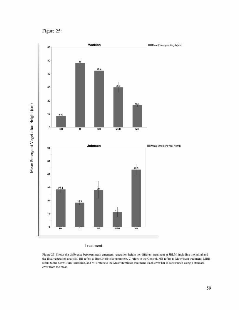
59
Figure 25:
Treatment
Figure 25: Shows the difference between mean emergent vegetation height per different treatment at JBLM, including the initial and the final vegetation analysis. BH refers to Burn/Herbicide treatment, C refers to the Control, MB refers to Mow/Burn treatment, MBH refers to the Mow/Burn/Herbicide, and MH refers to the Mow/Herbicide treatment. Each error bar is constructed using 1 standard error from the mean.
Mean Em
ergent Vegetation Heigh
t (cm
)
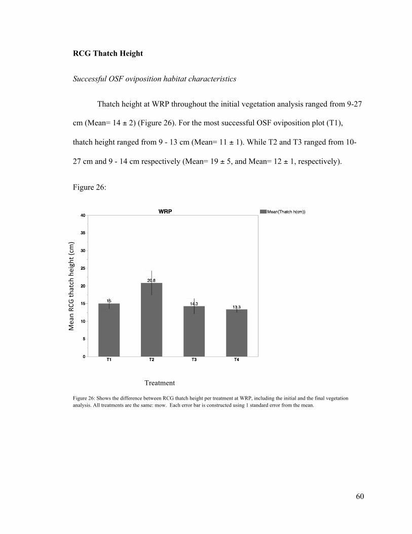
60
RCG Thatch Height
Successful OSF oviposition habitat characteristics
Thatch height at WRP throughout the initial vegetation analysis ranged from 9-27
cm (Mean= 14 ± 2) (Figure 26). For the most successful OSF oviposition plot (T1),
thatch height ranged from 9 - 13 cm (Mean= 11 ± 1). While T2 and T3 ranged from 10-
27 cm and 9 - 14 cm respectively (Mean= 19 ± 5, and Mean= 12 ± 1, respectively).
Figure 26:
Treatment
Figure 26: Shows the difference between RCG thatch height per treatment at WRP, including the initial and the final vegetation analysis. All treatments are the same: mow. Each error bar is constructed using 1 standard error from the mean.
Mean RC
G th
atch heigh
t (cm
)

61
Unsuccessful OSF oviposition habitat characteristics
Thatch height at Watkins ranged from 0 - 33 cm (Mean= 18 ± 3). The initial
vegetation analysis showed that the treatment with the lowest thatch height at this site
was the Mow/Burn/Herbicide treatment, ranging from 0 - 9 cm (Mean= 6 ± 3). Compared
to other treatments, the Control treatment had the highest mean thatch height ranging
from 30 - 33 cm (Mean= 32 ± 1), with the second highest one being the Mow/Burn
treatment that ranged from 7 - 30 cm (Mean= 22 ± 8) (Figure 27).
Thatch height at Johnson ranged from 11 - 61.5 cm (Mean = 35 ± 3). The
treatment with the lowest mean thatch height was the Mow/Burn/Herbicide plot ranging
from 11 - 42 cm (Mean= 29 ± 9). The Control treatment, which ranged from 16.5 - 48 cm
(Mean= 35 ± 9), was the plot with the second lowest thatch height (Figure 27).
The resampling ANOVA showed mean thatch height was significantly different
between Watkins and Johnson (SSamong= 2159.008, p= 0.0004). Further analysis
showed treatments were not significantly different from each other at both Watkins and
Johnson (SSamong= 871.6667, p=3857). When comparing treatments to the control plot,
none of the treatments significantly differed from the control for both Watkins and
Johnson.
Looking at the conditions where OSF has been successful, the treatments that had
similar thatch height averages to those at WRP were the Mow/Burn, Mow/Herbicide, and
Burn/Herbicide treatments at Watkins (Table 1). No treatments at Johnson were found
within the successful OSF oviposition range (Table 2).
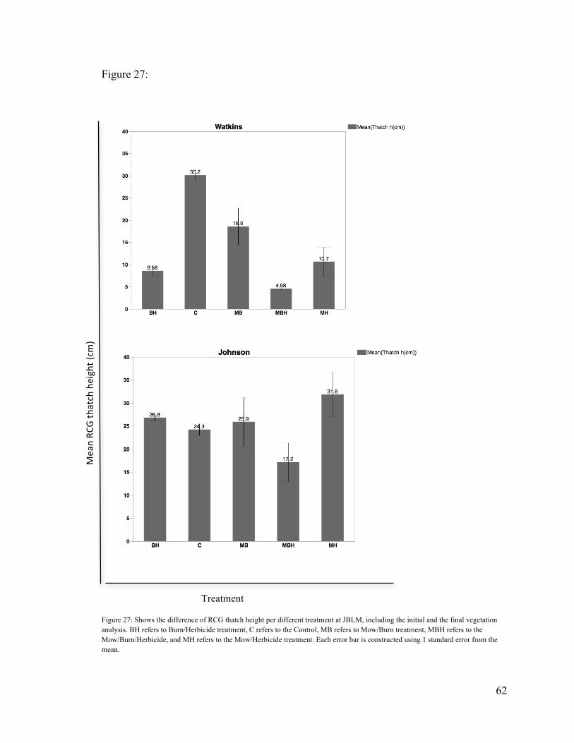
62
Figure 27:
Treatment
Figure 27: Shows the difference of RCG thatch height per different treatment at JBLM, including the initial and the final vegetation analysis. BH refers to Burn/Herbicide treatment, C refers to the Control, MB refers to Mow/Burn treatment, MBH refers to the Mow/Burn/Herbicide, and MH refers to the Mow/Herbicide treatment. Each error bar is constructed using 1 standard error from the mean.
Mean RC
G th
atch heigh
t (cm
)
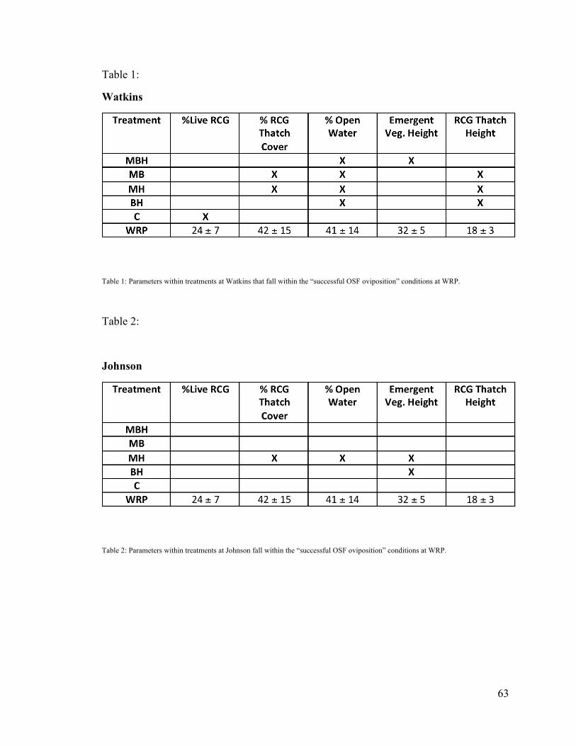
63
Table 1:
Watkins
Table 1: Parameters within treatments at Watkins that fall within the “successful OSF oviposition” conditions at WRP.
Table 2:
Johnson
Table 2: Parameters within treatments at Johnson fall within the “successful OSF oviposition” conditions at WRP.
64
CHAPTER 5: DISCUSSION
The main goal of this thesis was to see how ecological and hydrological
components of wetlands invaded with RCG could be improved by treating RCG, in order
to potentially restore OSF oviposition sites within JBLM. The different independent
variables (vegetation variables, hydrological variables, and chemical variables) were
chosen and monitored to examine individual effects they can have on OSF oviposition
site selection and success. The same metrics were measured at WRP in order to use as a
basis to compare a non-successful OSF oviposition habitat (in this case JBLM) to a
successful OSF oviposition habitat (WRP). This was done with the purpose of assessing
which treatment would allow for the independent variables to more closely resemble the
successful OSF oviposition site.
Results showed that treatments at JBLM affected all hydrologic, and most
vegetation components (except for thatch height), but no chemical components were
affected by the treatments. This suggests treatment of RCG can be utilized to manipulate
hydrologic and vegetation characteristics and potentially desired characteristics desired
by OSF throughout oviposition season.
65
Site differences
Egg mass data
Oviposition success was the main restoration focus on this study, since it is
necessary for OSF populations to be able to lay egg masses in order to have a self-
sustaining population. A total of 278 egg masses were found within the West Area of
WRP throughout the 2015 oviposition season. No egg masses were found within JBLM
both in 2014 and 2015, even with treatments being placed. This leads to question which
variables are limiting OSF oviposition at JBLM.
OSF is considered a sensitive species overall, subsequently it will also be a
sensitive species when it comes to selecting sites for oviposition. There are many
variables that can affect where the OSF chooses to lay egg masses, including vegetation
characteristics, hydrological conditions, and chemical conditions. This study looked at
these variables independently to identify patterns that are preferred by OSF for
oviposition site selection, and provide recommendations on management strategies for
wetlands infested with RCG.
It is important to point out that no adult OSF are usually found within the plots
being studied. Throughout the 2015 oviposition season there is only record of one frog
being observed within those sites (Within the Watkins site). This means that there is a
reason why OSF populations that have been released are not spending time at these sites.
It is currently not clear where the released frogs are spending time after being released.
Further studies are needed to address this question. If no adults are being found within the
66
sites, then it is not likely they will lay egg masses within the plots, even if the conditions
are ideal.
Chemical data
Conductivity
Conductivity levels were analyzed in this study since it has been hypothesized
conductivity levels can affect amphibian occupancy at breeding sites (Klaver, Peterson,
and Patla, 2013). It is not known to what level conductivity affects OSF specifically, but
since they are a sensitive species, it is possible that high conductivity levels might
prevent OSF from spending time at breeding sites and therefore reproducing there.
Results showed treatments did not significantly differed between sites at JBLM
(SSamong= 271.96, p= 0.1219), or between treatments within JBLM (either for Watkins
or Johnson). This suggests differences in conductivity levels aren’t attributed to
treatments but to specific site conditions.
Data analysis also showed there is much higher conductivity levels at JBLM
compared to WRP. SPC ranged from 69.1- 94.9, 68.7-104.6, and 19.5-103 µS/cm for
Watkins, Johnson, and WRP respectively (Mean= 85 ± 7; Mean= 90 ± 13; and Mean= 61
± 19; respectively). This can possibly be affecting OSF occupancy at potential
oviposition habitat within JBLM, and could be attributed to geological conditions or
specific activities surrounding the wetlands. While WRP is a nature reserve, with low
human traffic and no significant activity (other than recreational activities or scientific
research), JBLM is a facility with high human traffic and daily military operations. These

67
operations could potentially be affecting conductivity levels within wetlands at JBLM,
and potentially affecting OSF oviposition sites, but further study is necessary to confirm
this. This also leads to question if OSF prefers sites with lower conductivity levels.
Further study is required to identify the causes.
Dissolved Oxygen
Throughout this study it was hypothesized that treatments would affect DO
concentrations, since in theory excess in biomass could potentially have an effect on
oxygen available within the system. This variable was analyzed since DO concentrations
can affect productivity and biological activity within a wetland, possibly limiting OSF
reproductive activity within wetlands. There were no significant differences between sites
within JBLM (SSamong= 0.00841,p=0.9090). There were also no significant differences
between treatments. This suggests treatments, and therefore RCG, have no effect on DO
concentrations within these specific wetlands at JBLM. Moreover, dissolved oxygen
might be affected more by existing environmental conditions (such as source of water for
the wetlands) than RCG density at JBLM.
Analysis of DO data collected showed there was no significant difference between
WRP and JBLM averages. DO ranged from 3.7-12.4, 5.5-9.8, and 4.2-13 mg/L for
Watkins, Johnson, and WRP respectively (Mean= 7.6 ± 2; Mean= 7.6 ± 1; Mean= 8.8 ±
3; respectively). This suggest DO might not be the variable limiting OSF oviposition
within JBLM.
68
Hydrologic data
Temperature
Hydrologic data showed temperatures at successful OSF oviposition site (WRP)
were more stable and had less variation than temperatures at JBLM. Mean temperatures
in WRP had a 3.6°C variation (from 6.1 - 9.7 °C), while mean temperatures at Johnson
had an 8 °C variation (from 5.3 -13.4 °C), and a 5°C variation at Watkins (from 5.5-
10.7°C). For an OSF oviposition site high temperature variations can result in egg mass
mortality, especially if they reach low temperature levels. Temperatures below 6°C are
considered unfit for OSF oviposition, and can affect development of the embryo(White,
2002). Both Johnson and Watkins showed temperatures below 6°C throughout the lower
temperature ranges. This suggest some of the overnight temperatures throughout at JBLM
OSF oviposition period can lead to egg mass mortality. Moreover, one of the triggers for
OSF to start laying egg masses is for surface water to reach that 6°C threshold, and since
temperatures are still reaching levels below that threshold throughout oviposition season
at JBLM, it could potentially be one of the reasons why OSF is not laying egg masses
there.
One of the objectives of this study was to determine if the different treatments
affected surface water temperatures. The hydrological analysis showed there was a
significant difference in mean water temperatures between treatments for both Watkins
and Johnson JBLM (SSamong = 61.96, p = <0.0001; SSamong = 1460.07, p = <0.0001,
respectively). This suggests treatments actually affect water temperature within these
specific wetlands, and therefore the presence of high RCG densities has the ability to

69
affect water temperature. When it comes to water temperature, the Mow/Herbicide
treatment seemed to have the highest water temperatures at JBLM, possibly due to its
success in reducing vegetation height and significantly reducing RCG densities (which in
turn allow for sun light to directly access surface waters. This could potentially prevent
OSF mortality throughout periods of cold temperature.
Water Level Fluctuations
Hydrological data showed surface water depth at successful OSF oviposition sites
(WRP) was much higher and fluctuated less than surface water depth at JBLM. Surface
water depth at WRP fluctuated by 0.13 m at T1 and T2 and 0.16 m at T3 and T4 (from
0.83-0.96 m, and 0.29-0.41 m, respectively), while fluctuating by 0.36 m at Watkins
(from 0.16-0.52 m), and 0.56 m at Johnson (from 0.03-0.59 m). OSF seems to prefer
wetlands with higher surface water availability to lay eggs, possibly due to the fact that
low surface water levels can lead to egg mass dissection and mortality, and also make it
harder for OSF to move from oviposition site to oviposition site.
One of the objectives of this study was to determine if the different treatments
affected surface water fluctuations. Analysis of hydrological data showed there was a
significant difference in mean water fluctuations between treatments for both Watkins
and Johnson (SSamong = 43.0603, p = <0.0001; SSamong = 157.6803, p = <0.0001,
respectively). This suggests that the treatments have an effect on water level fluctuations;
therefore suggesting high RCG densities can have an effect on surface water depth for
these specific wetlands.
70
The treatments with highest water levels at JBLM were the Mow/Herbicide
treatment for Watkins (ranging from 0.37- 0.44 m). For the Johnson site the treatment
with the highest water level was the Control treatment, possibly due to shading from
RCG thatch. Following the control treatment at Johnson, the one with the second highest
water levels was the Mow/Herbicide treatment, ranging from 0.46-0.56 m. Since JBLM
has lower water levels, a treatment such as Mow/Herbicide that prevents water levels
from getting too low might be a good alternative.
Vegetation differences between treatments
Percentage live RCG
RCG has the ability to reproduce both vegetatively and sexually, therefore
presence of live RCG can lead to further infestation. Live RCG was measured with the
purpose on looking at how effective the treatments were at eradicating RCG overall.
Since RCG management practices (mowing once per year) at WRP have the purpose of
seasonally reducing RCG density and not necessarily eradicating it, it was expected to
find RCG at the site throughout oviposition season. Vegetation data analysis showed
mean live RCG percentages at WRP and Watkins were similar (Mean= 16 ± 4, and
Mean= 15 ± 5, respectively), while Johnson had a much lower live RCG percentage
(Mean = 4 ± 2). This suggests treatments were more efficient at completely eradicating
RCG at Johnson than at Watkins. When it comes to OSF oviposition, if an additional goal
is to eradicate RCG, it would be necessary to plant desired species to provide the habitat
that RCG is providing for OSF at WRP.
71
One of the objectives of this study was to see if the different treatments affected
percent live RCG within JBLM wetlands. Since analysis showed there was a significant
difference between treatments both at Watkins and Johnson (SSamong= 4532.3,
p=0.0002), it can be said that the different treatments had an effect on the percent of live
RCG found at these specific wetlands. This can benefit wetlands at JBLM if the
treatments are seeded or planted with desired species, in order to prevent RCG from
establishing at the sites again.
The treatment at JBLM that most resembled percent live RCG in OSF successful
oviposition conditions (specifically where egg masses were laid within WRP) was the
control site at Watkins. No treatment at Johnson fell within the range of “ideal
conditions”, possibly due to the success of treatments at eradicating RCG completely
Percentage RCG thatch cover
RCG thatch can be useful for OSF oviposition habitat, since it can provide
stability for egg mass deposition. Percentage RCG thatch cover was measured to see its
importance when it comes to OSF oviposition site selection. Overall there was a lower
percentage thatch cover both at Watkins and Johnson (Mean= 43 ± 8; Mean = 38 ± 10;
respectively) compared to WRP (Mean= 49 ± 10). This suggests treatments were
successful at eradicating RCG thatch, which can possibly affect OSF oviposition habitat
selection.
One objective of this study was to see if the different treatments had an effect on
percentage RCG thatch cover. Vegetation data analysis showed there was a significant

72
difference between treatments for both Watkins and Johnson (SSamong= 28692.9,
p<0.0001), suggesting the treatments had an effect on percentage RCG thatch cover
within these wetlands. These treatments can decrease RCG thatch cover, and with that
increase open water habitat, which is necessary for OSF to move between oviposition
sites.
The treatments at JBLM that most resembled percentage RCG thatch cover in
OSF successful oviposition conditions (specifically where egg masses were laid within
WRP) were the Mow/Burn, and Mow/Herbicide treatments at Watkins, and the
Mow/Herbicide treatment at Johnson. This can be attributed to the fact that these three
treatments were treated with mowing before a follow up mechanical or chemical
treatment, and all treatments at WRP have a mowing treatment.
Percentage open water
Open water is necessary throughout oviposition period, since it can provide OSF
movement between potential breeding sites. It can also prevent egg mass mortality due to
desiccation. Watkins had similar mean percent open water to treatments at WRP (Mean=
36 ± 9, and Mean= 35 ± 8; respectively), while Johnson had much higher percent open
water (Mean = 63 ± 10). This can be due to the fact that even though treatments at JBLM
were successful at eradicating RCG overall, new species colonization was observed at
Watkins, but it was lacking at Johnson.
Another objective of this study was to see if the different treatments had an effect
on percent open water available. Vegetation data analysis showed there was a significant
73
difference between treatments when it comes to mean percentage open water both at
Johnson and Watkins (SSamong= 22167.5, p= 0.0013), suggesting treatments were
successful at reducing RCG densities, or completely eradicating it, which in turn increase
open water habitat.
Emergent vegetation height
OSF tends to prefer habitats with low emergent vegetation height, since they look
for habitat where the sunlight can directly reach egg masses. Moreover, OSF tends to be a
very cryptic species, and is more partial to spending time where emergent vegetation can
provide protection from predators. Emergent vegetation height was similar at WRP and
JBLM, but the amount of vegetation available did. The treatment with the lowest mean
emergent vegetation height was the Burn/Herbicide treatment at Watkins (Mean= 8.4 ±
3), possibly due to the combination of methods that were effective at first removing
excess biomass by burning, and then eradicating RCG by applying herbicide.
Another objective of this study was to see if treatments had an effect on emergent
vegetation height. Results showed there was a significant difference between mean
emergent vegetation height between the treatments for both Watkins and Johnson
(SSamong= 3020.033, p= 0.0279). These results suggest these specific treatments are
effective at controlling emergent vegetation height, an can potentially help provide
habitat suitable for OSF oviposition, where sunlight is able to have direct contact with
egg masses, but protection from predators is also provided.

74
The treatments that most resembled “successful OSF oviposition conditions” were
the Mow/Burn/Herbicide treatment at Watkins, and the Mow/Herbicide, and
Burn/Herbicide treatment at Johnson. This suggests the use of herbicide might have an
effect on RCG growth within JBLM, and might be a desired approach within these
wetlands.
RCG Thatch height
Thatch height can affect OSF reproduction site selection, since they prefer
submerged vegetation in order to provide certain stability for egg masses. If thatch height
is too high it can lead to mortality by desiccation throughout low water periods, since it
can rise above the water table and prevent egg masses from being submerged. The
treatment with the lowest mean thatch height at JBLM was the Mow/Burn/Herbicide
treatment at Watkins (Mean= 4.58 ± 0.6). This could be due to the combination of
mechanical practices and chemical practices that were very efficient at eradicating live
RCG, dead RCG biomass, and preventing new RCG growth.
One of the purposes of this thesis is to see if treatments affected thatch height
within JBLM. Data analysis showed treatments did not affect thatch height within JBLM
(SSamong= 871.6667, p=0.3857). This suggests some treatments might be efficient at
completely eradicating RCG, but not as efficient at getting rid of dead biomass left
behind after RCG has been exterminated.
The treatment at JBLM that most resembled the average thatch height present at
WRP (Mean= 14 ± 2) was the Mow/Burn/Herbicide treatment at Johnson (Mean= 17.17±
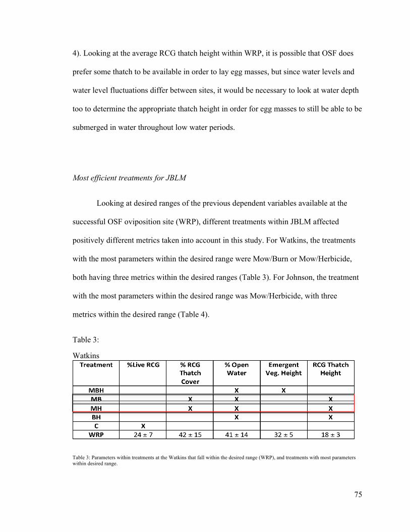
75
4). Looking at the average RCG thatch height within WRP, it is possible that OSF does
prefer some thatch to be available in order to lay egg masses, but since water levels and
water level fluctuations differ between sites, it would be necessary to look at water depth
too to determine the appropriate thatch height in order for egg masses to still be able to be
submerged in water throughout low water periods.
Most efficient treatments for JBLM
Looking at desired ranges of the previous dependent variables available at the
successful OSF oviposition site (WRP), different treatments within JBLM affected
positively different metrics taken into account in this study. For Watkins, the treatments
with the most parameters within the desired range were Mow/Burn or Mow/Herbicide,
both having three metrics within the desired ranges (Table 3). For Johnson, the treatment
with the most parameters within the desired range was Mow/Herbicide, with three
metrics within the desired range (Table 4).
Table 3:
Watkins
Table 3: Parameters within treatments at the Watkins that fall within the desired range (WRP), and treatments with most parameters within desired range.
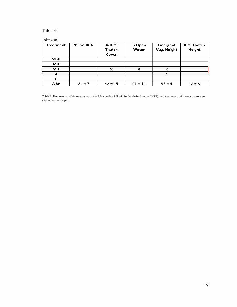
76
Table 4:
Johnson
Table 4: Parameters within treatments at the Johnson that fall within the desired range (WRP), and treatments with most parameters within desired range.
77
CHAPTER 6: RECOMMENDATIONS AND CONCLUSION
Treatments at JBLM were done with the purpose of seeing how the different
treatments (Mow/Burn/Herbicide, Mow/Burn, Mow/Herbicide, Burn/Herbicide, and
Control) affected RCG densities. This study focused on looking at conditions wetlands
were left in after treatments, and seeing if they could provide habitat for OSF for
oviposition purposes by comparing it to a “successful OSF oviposition site” (WRP). Egg
masses continue to be found only at WRP. This leads to question if the lack of egg
masses at JBLM is attributed to intrinsic site properties or surrounding activities that
prevent OSF from reproductive success at JBLM. So far, only one adult was observed
within the treated sites (Watkins), and no eggs were observed. As such, they appear to be
discriminating against this site with or without treatments. Looking at the different
metrics measured throughout the study, one of the site properties that could be affecting
OSF from establishing at JBLM might be high conductivity levels, or lower water levels,
or more water temperature fluctuations, but further research is necessary to understand
the cause.
Treatments within JBLM had an effect on all hydrologic components, and most of
vegetation components (except for thatch height). Chemical components were not
significantly affected by treatments, leading to believe that pre-existing site conditions or
current activities surrounding the wetlands might have more of an effect in chemical
properties than treatments at this specific wetlands (Watkins and Johnson) within JBLM.
The Mow/Burn/Herbicide treatment was the most effective at completely
eradicating RCG from Watkins and Johnson, but for the purpose of OSF ovipositon

78
habitat enhancement, the Mow/Herbicide treatment was the treatment that had the most
parameters within the desired range at JBLM. Complete RCG eradication would be ideal
if it is coupled with introduction of desired vegetation, since at this point it is RCG who
provides shading and stability needed for OSF oviposition periods. This leads to the
realization that wetlands invaded with RCG at JBLM can potentially be treated for OSF
oviposition success. This also gives rise to an opportunity for further research: How does
herbicide affect OSF throughout oviposition season? It would be important to know if
herbicide has some detrimental effects on OSF at different life stages before deciding to
use this treatment at large scale as a management strategy.
Finally, there are many ways invasive RCG can be treated depending on
management goals and resources available. This research helps stress the importance of
taking wetlands on a case by case scenario, since all wetlands examined throughout this
study had different hydrologic, vegetation and chemical features, which in turn can affect
the choice of management strategy. The effects treatments have on different wetlands can
vary depending on existing wetland characteristics. It is recommended thoroughly
studying intrinsic wetland conditions before creating a management plan, and applying
treatments for RCG control.
79
Bibliography
Adams, C. R., & Galatowitsch, S. M. (2005). Phalaris arundinacea (reed canary grass):
Rapid growth and growth pattern in conditions approximating newly restored
wetlands. Ecoscience, 12(4), 569–573. http://doi.org/10.2980/i1195-6860-12-4-
569.1
Apfelbaum, S. I., & Sams, C. E. (1987). Ecology and control of reed canary grass.
Natural Areas Journal, 7(2), 69.
Chelgren, N. D., Pearl, C. A., Adams, M. J., & Bowerman, J. (2008). Demography and
Movement in a Relocated Population of Oregon Spotted Frogs (Rana pretiosa):
Influence of Season and Gender. Copeia, 2008(4), 742–751.
http://doi.org/10.1643/CH-07-142
Denton, R. D., & Richter, S. C. (2013). Amphibian communities in natural and
constructed ridge top wetlands with implications for wetland construction.
Journal of Wildlife Management, 77(5), 886–896.
http://doi.org/10.1002/jwmg.543
Foster, R. D., & Wetzel, P. R. (2005). Invading monotypic stands ofPhalaris arundinacea:
A test of fire, herbicide, and woody and herbaceous native plant groups.
Restoration Ecology, 13(2), 318–324. http://doi.org/10.1111/j.1526-
100X.2005.00040.x
Hallock, L. E. (2013). Oregon Spotted Frog Recovery Plan, State of Washington
(DRAFT) (p. 106). Washington Department of Fish and Wildlife. Retrieved from
http://wdfw.wa.gov/publications/01505/wdfw01505.pdf
80
Herr-Turoff, A., & Zedler, J. B. (2007). Does morphological plasticity of the Phalaris
arundinacea canopy increase invasiveness? Plant Ecology, 193(2), 265–277.
http://doi.org/10.1007/s11258-007-9264-2
Hillhouse, H. L., Tunnell, S. J., & Stubbendieck, J. (2010). Spring Grazing Impacts on
the Vegetation of Reed Canarygrass-Invaded Wetlands. Rangeland Ecology &
Management, 63(5), 581–587. http://doi.org/10.2111/REM-D-09-00173.1
Iannone III, B. V., & Galatowitsch, S. M. (2008). Altering Light and Soil N to Limit
Phalaris arundinacea Reinvasion in Sedge Meadow Restorations. Restoration
Ecology, 16(4), 689–701. http://doi.org/10.1111/j.1526-100X.2008.00481.x
Jakubowski, A. R., Casler, M. D., & Jackson, R. D. (2010). Landscape Context Predicts
Reed Canarygrass Invasion: Implications for Management. Wetlands, 30(4), 685–
692. http://doi.org/10.1007/s13157-010-0078-y
Jenkins, N. J., Yeakley, J. A., & Stewart, E. M. (2008). First-Year Responses to Managed
Flooding of Lower Columbia River Bottomland Vegetation Dominated by
Phalaris Arundinacea. Wetlands, 28(4), 1018–1027.
Kaproth, M., Eppinga, M., & Molofsky, J. (2013). Leaf litter variation influences
invasion dynamics in the invasive wetland grass Phalaris arundinacea. Biological
Invasions, 15(8), 1819–1832. http://doi.org/10.1007/s10530-013-0411-5
Kapust, H. Q., McAllister, K. R., Hayes, M. P., & others. (2012). Oregon spotted frog
(Rana pretiosa) response to enhancement of oviposition habitat degraded by
invasive reed canary grass (Phalaris arundinacea). Herpetological Conservation
and Biology, 7(3), 358–366.
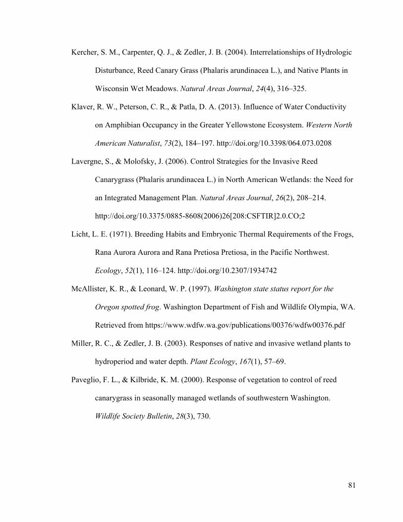
81
Kercher, S. M., Carpenter, Q. J., & Zedler, J. B. (2004). Interrelationships of Hydrologic
Disturbance, Reed Canary Grass (Phalaris arundinacea L.), and Native Plants in
Wisconsin Wet Meadows. Natural Areas Journal, 24(4), 316–325.
Klaver, R. W., Peterson, C. R., & Patla, D. A. (2013). Influence of Water Conductivity
on Amphibian Occupancy in the Greater Yellowstone Ecosystem. Western North
American Naturalist, 73(2), 184–197. http://doi.org/10.3398/064.073.0208
Lavergne, S., & Molofsky, J. (2006). Control Strategies for the Invasive Reed
Canarygrass (Phalaris arundinacea L.) in North American Wetlands: the Need for
an Integrated Management Plan. Natural Areas Journal, 26(2), 208–214.
http://doi.org/10.3375/0885-8608(2006)26[208:CSFTIR]2.0.CO;2
Licht, L. E. (1971). Breeding Habits and Embryonic Thermal Requirements of the Frogs,
Rana Aurora Aurora and Rana Pretiosa Pretiosa, in the Pacific Northwest.
Ecology, 52(1), 116–124. http://doi.org/10.2307/1934742
McAllister, K. R., & Leonard, W. P. (1997). Washington state status report for the
Oregon spotted frog. Washington Department of Fish and Wildlife Olympia, WA.
Retrieved from https://www.wdfw.wa.gov/publications/00376/wdfw00376.pdf
Miller, R. C., & Zedler, J. B. (2003). Responses of native and invasive wetland plants to
hydroperiod and water depth. Plant Ecology, 167(1), 57–69.
Paveglio, F. L., & Kilbride, K. M. (2000). Response of vegetation to control of reed
canarygrass in seasonally managed wetlands of southwestern Washington.
Wildlife Society Bulletin, 28(3), 730.
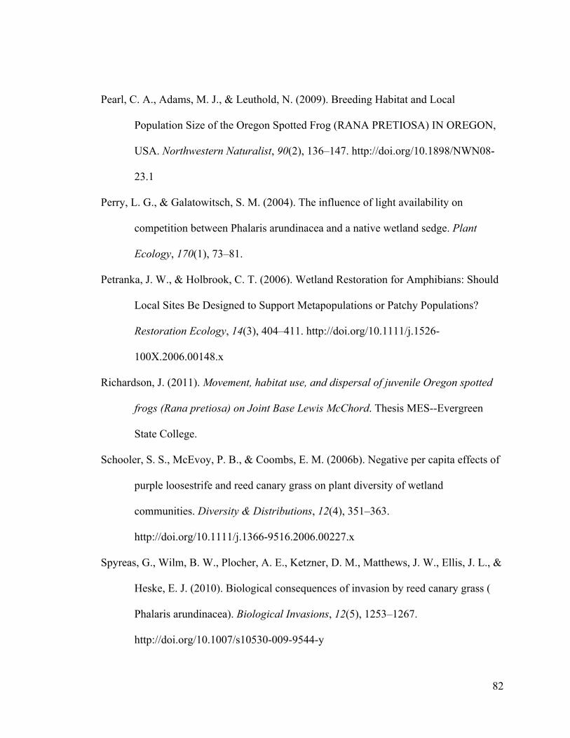
82
Pearl, C. A., Adams, M. J., & Leuthold, N. (2009). Breeding Habitat and Local
Population Size of the Oregon Spotted Frog (RANA PRETIOSA) IN OREGON,
USA. Northwestern Naturalist, 90(2), 136–147. http://doi.org/10.1898/NWN08-
23.1
Perry, L. G., & Galatowitsch, S. M. (2004). The influence of light availability on
competition between Phalaris arundinacea and a native wetland sedge. Plant
Ecology, 170(1), 73–81.
Petranka, J. W., & Holbrook, C. T. (2006). Wetland Restoration for Amphibians: Should
Local Sites Be Designed to Support Metapopulations or Patchy Populations?
Restoration Ecology, 14(3), 404–411. http://doi.org/10.1111/j.1526-
100X.2006.00148.x
Richardson, J. (2011). Movement, habitat use, and dispersal of juvenile Oregon spotted
frogs (Rana pretiosa) on Joint Base Lewis McChord. Thesis MES--Evergreen
State College.
Schooler, S. S., McEvoy, P. B., & Coombs, E. M. (2006b). Negative per capita effects of
purple loosestrife and reed canary grass on plant diversity of wetland
communities. Diversity & Distributions, 12(4), 351–363.
http://doi.org/10.1111/j.1366-9516.2006.00227.x
Spyreas, G., Wilm, B. W., Plocher, A. E., Ketzner, D. M., Matthews, J. W., Ellis, J. L., &
Heske, E. J. (2010). Biological consequences of invasion by reed canary grass (
Phalaris arundinacea). Biological Invasions, 12(5), 1253–1267.
http://doi.org/10.1007/s10530-009-9544-y
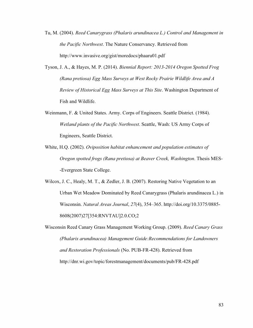
83
Tu, M. (2004). Reed Canarygrass (Phalaris arundinacea L.) Control and Management in
the Pacific Northwest. The Nature Conservancy. Retrieved from
http://www.invasive.org/gist/moredocs/phaaru01.pdf
Tyson, J. A., & Hayes, M. P. (2014). Biennial Report: 2013-2014 Oregon Spotted Frog
(Rana pretiosa) Egg Mass Surveys at West Rocky Prairie Wildlife Area and A
Review of Historical Egg Mass Surveys at This Site. Washington Department of
Fish and Wildlife.
Weinmann, F. & United States. Army. Corps of Engineers. Seattle District. (1984).
Wetland plants of the Pacific Northwest. Seattle, Wash: US Army Corps of
Engineers, Seattle District.
White, H.Q. (2002). Oviposition habitat enhancement and population estimates of
Oregon spotted frogs (Rana pretiosa) at Beaver Creek, Washington. Thesis MES-
-Evergreen State College.
Wilcox, J. C., Healy, M. T., & Zedler, J. B. (2007). Restoring Native Vegetation to an
Urban Wet Meadow Dominated by Reed Canarygrass (Phalaris arundinacea L.) in
Wisconsin. Natural Areas Journal, 27(4), 354–365. http://doi.org/10.3375/0885-
8608(2007)27[354:RNVTAU]2.0.CO;2
Wisconsin Reed Canary Grass Management Working Group. (2009). Reed Canary Grass
(Phalaris arundinacea) Management Guide:Recommendations for Landowners
and Restoration Professionals (No. PUB-FR-428). Retrieved from
http://dnr.wi.gov/topic/forestmanagement/documents/pub/FR-428.pdf