RESPONSES OF GREETING CARD ASSOCIATION WITNESS JAMES … · RESPONSES OF GREETING CARD ASSOCIATION...

BEFORE THE POSTAL RATE COMMISSION

WASHINGTON, D.C. 20268B0001 POSTAL RATE AND FEE CHANGES, 2006

Docket No. R2006-1

RESPONSES OF GREETING CARD ASSOCIATION WITNESS JAMES A. CLIFTON TO INTERROGATORIES OF THE UNITED

STATES POSTAL SERVICE (USPS/GCA-T1-56-63a., 64, 65, 67-70, and 72-80)

(October 27, 2006)

The Greeting Card Association (“GCA”) hereby provides the responses of

James A. Clifton to the following interrogatories of the United States Postal

Service filed on October 4, 2006: USPS/GCA T1-56-63a., 64, 65, 67-70 and 72-

80. Each interrogatory is set out verbatim followed by the response. Responses

to USPS/GCA T1-63b.-g., 66 and 71 will be forthcoming.

Respectfully submitted, /s/ James Horwood James Horwood Spiegel & McDiarmid 1333 New Hampshire Ave. NW 2nd Floor Washington, D.C. 20036

Date: October 27, 2006

Postal Rate CommissionSubmitted 10/27/2006 2:01 pmFiling ID: 54574Accepted 10/27/2006

RESPONSE OF GREETING CARD ASSOCIATION WITNESS CLIFTON TO INTERROGATORIES OF THE UNITED STATES POSTAL SERVICE

1 of 6

USPS/GCA-T1-56: You have stated in several places in your testimony and in your responses to USPS/GCA-T1-9, USPS/GCA-T1-33, and USPS/GCA-T1-42 that the non-linear transformation which witness Thress applies to consumption expenditures on Internet Service Providers in his testimony “is not a Box-Cox transformation.”

a. Please confirm that witness Thress’s model can be expressed as follows: Ln(V) = a + b(Xλ) + …

b. Please confirm that a Box-Cox model can be expressed as follows: Ln(V) = a’ + b’[(Xλ – 1) / λ] + …

c. Please confirm that the Box-Cox model equation in b. could be re-written as follows:

Ln(V) = a’ + (b’/λ)(Xλ) – (b’/λ) + … d. Please confirm that the Box-Cox model equation in c. could be re-written

as follows: Ln(V) = [a’ – (b’/λ)]+ (b’/λ)(Xλ) + …

e. Please confirm that the Box-Cox model equation in d. could be re-written as follows:

Ln(V) = a + b(Xλ) + … Where a = a’ – (b’/λ) and b = (b’/λ)

f. Please confirm that witness Thress’s model equation in a. is identical to the Box-Cox model equation in e.

g. Please confirm that your statements that witness Thress’s transformation “is not a Box-Cox transformation” (e.g., page 31, line 3 of your testimony) are not correct.

h. Would the fact that witness Thress does, in fact, use a correct Box-Cox transformation in his work change your answer to USPS/GCA-T1-33?

i. Would the fact that witness Thress does, in fact, use a correct Box-Cox transformation in his work change your answer to USPS/GCA-T1-42?

RESPONSE:

a-i. Please see Dr. Kelegian’s response to USPS/GCA-2, redirected to GCA

witness Kelejian. Before I continue, I should make it clear that, Mr. Thress

nowhere in his testimony shows or states that he has reformulated the Box-Cox

transformation. In addition to Dr. Kelejian’s response and assuming that Mr.

Thress has deliberately reformulated his Box-Cox specification, I will show below

2 of 6

that this reformulation of Box-Cox in R2006-1 has resulted in two relevant

variables being omitted from his model. This results in a mis-specified model.

This can introduce serious bias in the model with severe consequences.

To begin with, let’s write the complete Internet variables in the Single-Piece

equation for R2006-1 with the correct Box-Cox specification:

L(n) = a0 + (b0+b1*T1+b2*T2)(ISP^ λ -1)/λ

Where T1=Trend, T2=T02Q4, and ISP=CS_ISP

Let’s reformulate this specification and re-group relevant terms:

L(n) = [(a0-b0/λ)] + [(b0/λ +b1/λ*T1+b2/λ*T2)*(ISP^ λ)] + [(-b1/λ)*T1+(-b2/λ)*T2)]

Let a0’ = a0-b0/λ in the first bracket; b0’ = b0/λ, b1’ = b1/λ, and b2’ = b2/λ in the

second bracket; and c1’ = b1/λ, and c2’ = b2/λ in the third bracket. Now we get:

L(n) = [a0’] + [(b0’+b1’ *T1+b2’ *T2)*(ISP^ λ)] + [c1*T1+c2*T2]

Below I have provided Thress’s Single-Piece equation given in LR-L-64, file,

demandequations.prg:

equation singlepiece2.ls bgvol01sp = c01sp(1) + c01sp(2)*employ(-1) + c01sp(3)*empl_t(-1) + (c01sp(4)+c01sp(26)*trend+c01sp(25)*t02q4)*(cs_isp^lcoef(1)) + c01sp(7)*msadj + c01sp(8)*mc95 + c01sp(9)*d2004_05q1 + x_d*d1_3ws + c01sp(10)*px01sp + c01sp(11)*px01sp(-1) + c01sp(12)*sep1_15 + c01sp(13)*sep16_30 + c01sp(14)*(oct+nov1_dec10) + c01sp(15)*(dec11_12+dec13_15+dec16_17+dec18_19) + c01sp(16)*(dec20_21+dec22_23+dec24) + c01sp(17)*(dec25_jan1+jan_feb) + c01sp(18)*march + c01sp(19)*apr1_15 + c01sp(20)*apr16_may + c01sp(22)*gqtr1 + c01sp(23)*gqtr2 + c01sp(24)*gqtr3 + (0-c01sp(22)-c01sp(23)-c01sp(24))*gqtr4 + 100000000*(lcoef(1) - @abs(lcoef(1))) + 100000000*((1-lcoef(1)) - @abs(1-lcoef(1)))

Comparing the correctly reformulated Box-Cox specification with Mr. Thress’s

reformulated Box-Cox, the terms in the second bracket are similar to those that

Mr. Thress has given in his equation. However, those terms in the third bracket,

3 of 6

that is, the two time trend variables of T1 & T2 are missing from Thress’s

demand equation above. To be considered a correctly reformulated Box-Cox

specification, these two relevant variables must be explicitly included in this

equation. Given that these two relevant time trend variables are omitted, Mr.

Thress’s model is mis-specified, thus, leading to biased estimates. (Please see

William H. Greene, Econometric Analysis, 1993, Second Edition, Macmillan

Publishing Company, New York, section 8.4.2 “Omission of Relevant Variables,

pages 245-247.)

What are the empirical consequences of Thress’s omitted variables? I did a

preliminary investigation by adding the two trend variables of TREND and T02Q4

to Mr. Thress’s equation above and re-estimated the model using his program

given in LR-L-64. Table One provides partial output for the correctly

reformulated Box-Cox transformation as well as Mr. Thress’s original estimation

in Panels A & B, respectively.

Coefficients Std. Error T-Ratio Coefficients Std. Error T-RatioCONSTANT 0.59774 0.20964 2.85129 0.01562 0.12514 0.12482EMPLOY(-1) 1.01400 0.33120 3.06157 0.67930 0.10804 6.28755EMPL_T(-1) -0.00780 0.00322 -2.42465 -0.00221 0.00079 -2.79245CS_ISP_L01SP 0.69108 0.06837 10.10860 0.75321 0.04588 16.41696CS_ISP_L01SP_T -0.00856 0.00089 -9.58340 -0.01109 0.00058 -19.00949CS_ISP_L01SP_T02 0.12634 0.01335 9.46331 -0.00814 0.00171 -4.76793MSADJ 0.01766 0.00523 3.37763 0.02046 0.00795 2.57555MC95 0.02917 0.01594 1.83019 0.05861 0.01076 5.44669D2004_05Q1 0.03946 0.01526 2.58561 0.04349 0.01496 2.90700D1_3WS 0.01567 0.05529 0.28333 -0.09566 0.00993 -9.63352TREND -0.00625 0.00251 -2.48955T02Q4 -0.09542 0.00938 -10.17524PX01SP -0.27598 0.11929 -2.31360 -0.07115 0.10636 -0.66891lag1 -0.05596 0.08192 -0.68310 -0.11259 0.10189 -1.10501lag2 0 0 0 0 0 0lag3 0 0 0 0 0 0lag4 0 0 0 0 0 0

Own Price Elasticity -0.331938 -0.18374

Table OneSingle-Piece Letters Demand Equation: 1983:1-2005:4

Box-Cox Transformation

Panel AThress's Model with Correctly Reformulated Thress''s Original Model

Panel B

4 of 6

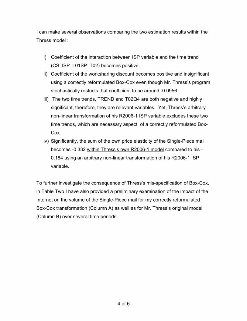
I can make several observations comparing the two estimation results within the

Thress model :

i) Coefficient of the interaction between ISP variable and the time trend

(CS_ISP_L01SP_T02) becomes positive.

ii) Coefficient of the worksharing discount becomes positive and insignificant

using a correctly reformulated Box-Cox even though Mr. Thress’s program

stochastically restricts that coefficient to be around -0.0956.

iii) The two time trends, TREND and T02Q4 are both negative and highly

significant, therefore, they are relevant variables. Yet, Thress’s arbitrary

non-linear transformation of his R2006-1 ISP variable excludes these two

time trends, which are necessary aspect of a correctly reformulated Box-

Cox.

iv) Significantly, the sum of the own price elasticity of the Single-Piece mail

becomes -0.332 within Thress’s own R2006-1 model compared to his -

0.184 using an arbitrary non-linear transformation of his R2006-1 ISP

variable.

To further investigate the consequence of Thress’s mis-specification of Box-Cox,

in Table Two I have also provided a preliminary examination of the impact of the

Internet on the volume of the Single-Piece mail for my correctly reformulated

Box-Cox transformation (Column A) as well as for Mr. Thress’s original model

(Column B) over several time periods.

5 of 6

Column A Column BReformulated Thress's

Box-Cox Model Original Model

Coefficients CoefficientsCS_ISP 0.691079 0.75321CS_ISP*T -0.008557 -0.01109CS_ISP*T02Q4 0.126344 -0.00814Box-Cox 0.145734 0.122

Period CS_ISP Trend T02Q4 ISP-Impact ISP-Impact1983Q1 0.0000000 49 0 0.00000 0.000001988Q2 0.0000451 70 0 0.02142 -0.00674

2000GQ1 0.0409519 117 0 -0.19465 -0.368172002GQ3 0.0637703 127 0 -0.26492 -0.467852002GQ4 0.0632438 128 1 -0.18583 -0.481102003GQ1 0.0655523 129 2 -0.10762 -0.497002004GQ1 0.0786080 133 6 0.21472 -0.564522004GQ2 0.0791217 134 7 0.29631 -0.579082004GQ3 0.0821951 135 8 0.37980 -0.595952004GQ4 0.0818597 136 9 0.46136 -0.609822005GQ1 0.0826809 137 10 0.54394 -0.624742005GQ2 0.0852990 138 11 0.62870 -0.641362005GQ3 0.0874551 139 12 0.71357 -0.657602005GQ4 0.0895049 140 13 0.79885 -0.67378

Impact of Internet on the Volume of Single-Piece Mail LettersR2006-1

Table Two

As it is shown in Table Two, using Box-Cox, the impact of the internet on the

single-piece volume is initially positive, then becomes negative and then

becomes positive again beginning in 2004GQ1. These results are at odds with

the economic reality surrounding the Internet’s impact on mail but they are the

results of using a correctly reformulated Box-Cox.

There are three non-exclusive possibilities as to why Mr. Thress used the R2006-

1 non-linear form (ISPλ) form that he used:

(1) Erroneous understanding of the Box-Cox transformation or erroneous Box-

Cox “reformulation”.

6 of 6

(2) Intentionally choosing his non-linear form (ISPλ) rather than properly

specified Box-Cox transformation [(Xλ – 1)/λ], because he could not obtain

empirical results that were plausible with the latter.

(3) An arbitrary choice on this particular variable.


1 of 1

USPS/GCA-T1-57: In your response to USPS/GCA-T1-42, you indicate that you believe that “[i]ncluding a variable as non-linear without some reasonable justification is nothing but an arbitrary choice.” At line 3 of page 18 of your testimony you present the following hypothetical equation for modeling the demand for First-Class single-piece letters.

(2) log(Q) = a – b log(P) + b2 log(P2) where P is the price of First-Class single-piece letters and P2 is the price of competing electronic alternatives. You go on to state that “price data for competing substitutes … is not readily available.”

a. Would it be appropriate in this case to attempt to find some variable, call it z, to serve as a proxy for log(P2) within equation (2)? If not, why not?

b. Suppose that there was some variable, X, and some constant, y, such that Xy appeared to be very highly correlated with log(P2). Would it be appropriate in this case to substitute Xy into equation (2) as a proxy for log(P2)? If not, why not?

c. If Xy as described in part b. were used instead of log(P2) in equation (2), would the estimated value of b be biased? If so, please provide the precise mathematical formulation for the expected value of b expressed as a function of the true value of b?

d. If X (not raised to the power y) as described in part b. were used instead of log(P2) in equation (2), would the estimated value of b be biased? If so, please provide the precise mathematical formulation for the expected value of b expressed as a function of the true value of b?

RESPONSE:

a-d. Please see Dr. Kelejian’s response to USPS/GCA-3 redirected to GCA

witness Kelejian.


1 of 1

USPS/GCA-T1-58: In your response to USPS/GCA-T1-1(c), you say that witness Thress’s own-price elasticity estimate is “biased” because “the Box-Cox specification … dampens the true estimates.”

a. Please confirm that it is possible for two unbiased estimates to have different values. Further, please confirm that if two estimates are different, this does not necessarily mean that either of the two estimates is “biased” as you define that term in your response to USPS/GCA-T1-1(a).

b. Why was the “Box-Cox specification of the ISP variable” used by witness Thress “incorrect and unnecessary”?

c. What is the specific bias which is introduced through witness Thress’s use of the “Box-Cox specification of the ISP variable”? In your answer, please provide a precise mathematical formula for the expected value of the own-price elasticity from witness Thress’s equation. If you are unable to provide such a formula, please explain how you can state with certainty that witness Thress’s own-price elasticity is “biased” as you define that term in your answer to USPS/GCA-T1-1(a).

d. What is the basis for your assertion in your answer to USPS/GCA-T1-1(c) that “even if Box-Cox is correctly specified, its coefficients should be estimated along with the other coefficients using an appropriate econometric technique such as the maximum-likelihood estimation rather than least square technique. Otherwise, this could also be another source of bias.”

RESPONSE:

a. Confirmed for both.

b. Please see my response to USPS/GCA-T1-56. Furthermore, there are

plausible justifications for entering the ISP variable in a linear form as I do in

my VES model.

c. Please see my response to USPS/GCA-T1-56 and the reference to Greene.

d. Please see Dr. Kelejian’s response to USPS/GCA-10, redirected to GCA

witness Kelejian.


1 of 2

USPS/GCA-T1-59: In your response to USPS/GCA-T1-2, you state that “the definition of the U.S. payments market I adopt is based on that of the 2004 Federal Reserve Bank of Atlanta study.”

a. Please confirm that the “U.S. payments market” as defined in the 2004 Federal Reserve Bank of Atlanta study includes non-cash transactions made at the point of sale. For example, point-of-sale transactions are cited specifically on pages 4, 5, and 6 of this report.

b. Please confirm that point-of-sale transactions would not have ever been sent through the mail. If you cannot confirm, please give an example of a point-of-sale transaction which would involve payment being sent through the mail.

c. Please confirm that the greatest increases in non-cash payments identified in the Federal Reserve’s report were for credit cards and debit cards.

d. Please confirm that the vast majority of credit card and debit card payments represent point-of-sale transactions. If you cannot confirm, please provide the basis for your position.

e. Since credit cards and debit cards are used primarily for point-of-sale transactions, and point-of-sale transactions would never have been sent through the mail, what would you expect the increase in the use of credit cards and debit cards to make point-of-sale transactions to be on the volume of First-Class Mail? Please explain fully.

RESPONSE:

a. – e. You are missing the forest for the trees. The Postal Service has

repeatedly underestimated the size of the U. S. Payments market in studies such

as the annual Household Diary Study, with the result that its share of that market

is made to look substantially larger than it actually is. Incredibly, even the latest

available 2005 Diary did not include debit cards as a bill payment method even

though the 2004 Atlanta FED study indicates that debit card payments were

nearly as large as credit card payments in 2003, 16 versus 19 billion respectively.

There is no explicit reference to “point of sale” transactions anywhere on pages

4-6 except page 5 with reference to consumer checks being converted into

electronic payments. Unless you define point of sale transactions as those that

would never have been sent through the mail, a reductio ad absurdum

2 of 2

proposition, then no, I do not confirm your query in b. Many of these transactions

have involved the mail in some way in the past: older department store cards, for

example, or layaway plans, that involved bills sent by mail and payments made

by mail, as well as monthly bank statements sent by mail which included checks

processed for various transactions and payments. I do confirm that debit cards

were the fastest growing non-cash payment method in Exhibit 1 of the 2004 FED

study but do not confirm that credit cards showed one of the two greatest

increases. Credit cards were the second slowest growing means of non cash

payments in that Exhibit 1.


1 of 1

USPS/GCA-T1-60: In your response to USPS/GCA-T1-3, you define “pricing power” as “an economic term referring to the effect that a change in a firm’s production price has on the quantity demanded of that product.” On page 4, line 1, of your testimony you make the following assertion. “The facts are the Postal Service has no remaining ‘pricing power’ in [the U.S. payments] market[], where its correctly measured market share is well under 50%.”

a. Do you believe that the Postal Service had a “correctly measured market share” greater than 50% in the U.S. payments market at one time? Please provide the basis for your answer.

b. You state in your answer to USPS/GCA-T1-3 that “[p]ricing power relates to the “Price Elasticity of Demand.” Do you believe that the “Price Elasticity of Demand” has changed for First-Class Mail within the U.S. payments market? Please provide all of the evidence upon which you base your answer.

RESPONSE:

a. Yes. In addition to the payments instruments listed in the 2004 Atlanta FED

study, please refer to annual Household Diary Study tables such as Table 4.12 in

the 2005 study. In addition to “Mail”, the other payments instruments listed are

either relatively recent competitors to the mail, or insignificant, or both. Before

automatic deduction, the Internet, the credit card, the ATM, etc., mail appears

clearly to have been more dominant in the payments market than it is today.

b. Yes. See Table 3 on page 20 of my testimony, and the requested revisions to

that table provided to the Postal Service in my response to USPS/GCA-T1- 49.


1 of 5

USPS/GCA-T1-61: In your response to USPS/GCA-T1-44, you confirm that your First-Class single-piece letters equation includes the volume of First-Class single-piece letters lagged two quarters as an explanatory variable.

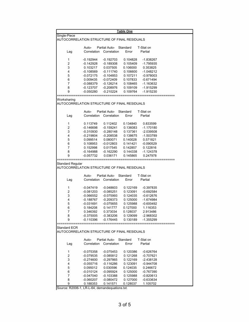
a. In your answer to USPS/GCA-T1-44(b), you say that witness Thress’s “econometric program is incapable of dealing with the autocorrelation problems.” What do you mean by this statement? Please provide all statistical evidence to suggest that witness Thress’s econometric program has failed to adequately deal with autocorrelation in his equations.

b. In your response to USPS/GCA-T1-44(b), you say that “Autocorrelation and partial autocorrelation that Mr. Thress has provided … reveals that his econometric program is incapable of dealing with the autocorrelation problems.” In his testimony on page 321, at line 3, Mr. Thress says that “a 95 percent confidence level is used to test for the presence of autocorrelation.” Please confirm that the partial autocorrelation values associated with First-Class single-piece letters presented by witness Thress in his output file, demandequations.txt, in LR-L-64, are not significant at a 95 percent confidence level. If not confirmed, please explain fully.

c. In your answer to USPS/GCA-T1-44(b), you state that with respect to witness Thress’s demand equations “in most cases the calculated Durbin Watson values are in the indeterminant range of critical values.” Please confirm that a Durbin Watson value “in the indeterminant range” is not evidence of autocorrelation. If not confirmed, please explain fully.

d. In the third edition of Econometric Analysis by William H. Greene (1997), on page 586, the author says, “If the regression contains any lagged values of the dependent variable, least squares will no longer be unbiased or consistent.” In your response to USPS/GCA-T1-47(a) you confirm that your demand equation for First-Class single-piece letters presented in Table A-8 of your testimony includes a lagged value of the dependent variable. Please confirm that your elasticity estimates from this equation are therefore biased and inconsistent. If not confirmed, please explain fully.

RESPONSE:

a. Please see Dr. Kelejian’s response to USPS/GCA-11 redirected to GCA

witness Kelejian. In addition to Dr. Kelejian’s response, below in Table One, I

have provided several examples of the final autocorrelation tables given in

Thress’ USPS-LR-L-64, file, demandequations.txt. It is evident from this table

that, in each case, one to several lags have significant autocorrelation at less

than a 10% significance level. For example, in the case of Single-Piece

2 of 5

equation, lags 1, 2, 8, and 9 are significant. In the case of Standard A Regular,

lag 3 is significant. In the Worksharing equation lag 3 is significant at 5% level.

In the case of Standard ECR, lag 3 is significant at less than 5% significance

level and etc. In summary, in the majority of mail category equations in the

Thress forecasting model, one to several autocorrelation lags are significant.

To illustrate the issue by way of examples, we used the Correlogram

autocorrelation procedure in Eviews and applied it to the residuals for Single-

Piece and Standard A Regular. These residuals are given in USPS-LR-L-64, file,

demandequations.txt. The Q-statistics tests are presented in Table two. The

tests confirm that Thress’s autocorrelation procedure has not removed all the

autocorrelation.

3 of 5

Single-PieceAUTOCORRELATION STRUCTURE OF FINAL RESIDUALS Auto- Partial Auto- Standard T-Stat on Lag Correlation Correlation Error Partial 1 -0.192944 -0.192703 0.104828 -1.838267 2 -0.142928 -0.189308 0.105409 -1.795935 3 0.103217 0.037505 0.106000 0.353825 4 -0.108569 -0.111740 0.106600 -1.048212 5 -0.072175 -0.104853 0.107211 -0.978003 6 0.009435 -0.072409 0.107833 -0.671494 7 -0.088379 -0.126214 0.108465 -1.163632 8 -0.123707 -0.208976 0.109109 -1.915299 9 -0.050280 -0.210224 0.109764 -1.915230 ===============================================================WorksharingAUTOCORRELATION STRUCTURE OF FINAL RESIDUALS Auto- Partial Auto- Standard T-Stat on Lag Correlation Correlation Error Partial 1 0.113749 0.112402 0.134840 0.833599 2 -0.146698 -0.159241 0.136083 -1.170180 3 -0.310930 -0.280148 0.137361 -2.039508 4 -0.219804 -0.208538 0.138675 -1.503789 5 0.099514 0.080071 0.140028 0.571821 6 0.108953 -0.012803 0.141421 -0.090529 7 0.152998 0.017545 0.142857 0.122816 8 -0.164988 -0.162290 0.144338 -1.124378 9 -0.057732 0.036171 0.145865 0.247978 ===============================================================Standard RegularAUTOCORRELATION STRUCTURE OF FINAL RESIDUALS Auto- Partial Auto- Standard T-Stat on Lag Correlation Correlation Error Partial 1 -0.047419 -0.048603 0.122169 -0.397835 2 -0.081203 -0.085251 0.123091 -0.692584 3 -0.066552 -0.075993 0.124035 -0.612676 4 -0.188767 -0.209373 0.125000 -1.674984 5 -0.031691 -0.075655 0.125988 -0.600492 6 0.184208 0.141777 0.127000 1.116353 7 0.346392 0.373034 0.128037 2.913486 8 -0.375005 -0.383206 0.129099 -2.968302 9 -0.110396 -0.176445 0.130189 -1.355299 ===============================================================Standard ECRAUTOCORRELATION STRUCTURE OF FINAL RESIDUALS Auto- Partial Auto- Standard T-Stat on Lag Correlation Correlation Error Partial 1 -0.075358 -0.075453 0.120386 -0.626764 2 -0.079535 -0.085812 0.121268 -0.707621 3 -0.274600 -0.297865 0.122169 -2.438128 4 -0.055716 -0.116286 0.123091 -0.944708 5 0.095012 0.030596 0.124035 0.246672 6 -0.010124 -0.095924 0.125000 -0.767390 7 -0.047040 -0.103388 0.125988 -0.820613 8 -0.060207 -0.080472 0.127000 -0.633634 9 0.188353 0.141571 0.128037 1.105702 Source: R2006-1, LR-L-64, demandequations.txt.

Table One

4 of 5

Lag AC PAC Q-Stat Prob AC PAC Q-Stat Prob

1 -0.193 -0.193 3.525 0.060 -0.046 -0.046 0.152 0.6972 -0.142 -0.186 5.453 0.065 -0.079 -0.081 0.601 0.7403 0.102 0.037 6.468 0.091 -0.065 -0.073 0.907 0.8244 -0.107 -0.110 7.589 0.108 -0.182 -0.199 3.380 0.4965 -0.071 -0.102 8.090 0.151 -0.031 -0.070 3.451 0.6316 0.009 -0.072 8.098 0.231 0.172 0.132 5.721 0.4557 -0.085 -0.126 8.827 0.265 0.315 0.324 13.461 0.0628 -0.118 -0.201 10.258 0.247 -0.331 -0.348 22.134 0.0059 -0.048 -0.207 10.495 0.312 -0.096 -0.122 22.873 0.006

10 0.126 -0.012 12.177 0.273 -0.128 -0.103 24.226 0.00711 -0.038 -0.097 12.331 0.339 -0.048 0.065 24.416 0.01112 -0.175 -0.302 15.634 0.209 0.169 0.046 26.849 0.00813 0.172 -0.090 18.887 0.127 0.066 -0.124 27.226 0.01214 0.111 0.005 20.252 0.122 0.077 0.038 27.743 0.01515 0.041 0.055 20.444 0.156 -0.303 -0.111 35.984 0.00216 -0.060 -0.166 20.849 0.184 -0.082 -0.105 36.606 0.00217 0.031 -0.075 20.957 0.228 0.015 0.008 36.628 0.00418 -0.066 -0.117 21.462 0.257 0.107 0.032 37.722 0.00419 0.053 -0.009 21.791 0.295 0.163 0.036 40.311 0.00320 0.010 -0.096 21.802 0.351 -0.164 -0.263 42.976 0.00221 -0.092 -0.132 22.830 0.353 0.098 0.162 43.955 0.00222 0.042 0.045 23.044 0.399 -0.218 0.013 48.855 0.00123 0.005 -0.022 23.047 0.458 0.056 0.020 49.188 0.00124 -0.079 -0.183 23.838 0.471 0.122 -0.102 50.811 0.001

CorrelogramThress's Single-Piece Residuals ress's Standrad Regular Residu

Table Two

b. Confirmed. First, arguably, using a 95% confidence level is somewhat too

restrictive. Second, in the four examples I have shown above in Table One,

some lags are significant at less that 95% (lag3 in worksharing, lag7 & lag8 in

standard regular and etc.), while others are significant at a little more than 95%

confidence level (lag1, lag2, lag8 & lag9 in single-piece).

c. Confirmed. A Durbin Watson value “in the indeterminant range” is not

evidence of autocorrelation. However, when this happens one needs to perform

further testing. The Q-Statistics test given above is an example of such tests,

which confirms the presence of autocorrelation in the Single-Piece and the

Standard A Regular models.

5 of 5

d. The paragraph from Greene you quote is totally out of context in this section

of his text book. You need to read the whole section including, in particular, the

last paragraph. What this section says is that if one has a model with the lag

dependent variable ( Yt = Yt-1 + εt ) and its residuals are correlated ( εt = ρ εt-1 + ut

) then using OLS leads to inconsistent and biased results. Otherwise, if the error

terms are not correlated, then, OLS is fine. The following table provides Q-

statistics for my Single-Piece linear model obtained using the Correlogram

procedure in the Eviews on the residuals.

lag AC PAC Q-Stat Prob1 0.094 0.094 0.847 0.3582 -0.002 -0.011 0.847 0.6553 0.211 0.214 5.156 0.1614 -0.063 -0.110 5.543 0.2365 -0.089 -0.068 6.331 0.2756 -0.034 -0.071 6.450 0.3757 -0.157 -0.121 8.949 0.2568 -0.160 -0.116 11.590 0.1709 -0.057 -0.031 11.927 0.217

10 0.088 0.151 12.736 0.23911 -0.107 -0.110 13.961 0.23512 -0.109 -0.119 15.256 0.22813 0.082 0.014 15.990 0.25014 -0.007 0.005 15.996 0.31415 0.113 0.143 17.438 0.29316 0.065 -0.032 17.918 0.32917 0.172 0.220 21.321 0.21218 0.081 -0.013 22.092 0.22819 0.030 -0.006 22.198 0.27520 -0.068 -0.205 22.748 0.30121 -0.193 -0.165 27.288 0.16222 -0.091 0.024 28.319 0.16523 -0.046 0.020 28.581 0.19524 -0.140 0.008 31.083 0.151

Correlogram for our Single-Piece Linear ModelTable One

My linear Single-Piece model has a lag-dependent variable in it and as the above

table shows, the residuals for it are not autocorrelated. Therefore, the OLS

technique is appropriate for my model, but witness Thress’s program has not

eliminated autocorrelation in his model.


1 of 1

USPS/GCA-T1-62: USPS/GCA-T1-15(c), asked the following: “If the percentage

of checks which are mailed, as opposed to being used at the point of sale, has

been increasing over time, could the number of checks which are mailed have

increased even as the total number of checks has decreased?”

a. If a variable, A, increases over time, and a variable, B, decreases over time, please confirm that the product of these two variables, A*B, could increase or decrease over time, depending on the specific values of A and B. If not confirmed, please explain fully.

b. Let A = the percentage of checks which are mailed, as opposed to being used at the point of sale. Let B = the total number of checks. Please confirm that the number of checks which are mailed would be equal to A*B. If not confirmed, please explain fully.

c. Please confirm that, if A has been increasing over time and B has decreased, that the value of A*B could have increased over time. If you cannot confirm, please reconcile your answer to your answer to part a.

d. Please confirm that the answer to USPS/GCA-T1-15(c) is “Yes.” If you cannot confirm, please reconcile your answer to your answer to parts a – c. above.

RESPONSE:

You are attempting to make a mathematical point, completely outside the actual

factual context, that hypothetically, even if overall check volumes are in decline,

checks sent through the mail could still be increasing. Yet, the Postal Service’s

own bill payment data from annual Household Diary studies contradicts your

hypothetical! It shows bill payments made by mail per month have dropped from

8.6 in FY2002 to 8.0 in FY2005. Since bill payments made by mail almost always

include a check, a decline in such mail means a decline in the number of checks

that are mailed.


1 of 2

USPS/GCA-T1-63: In your response to USPS/GCA-T1-16, you quote Dennis Carlton and Jeffrey Perloff, “All else the same, the larger a cross-elasticity of demand, the larger in absolute value is the direct elasticity of demand.”

a. Please confirm that Carlton and Perloff are talking about true (i.e., not estimated) price elasticities under long-run equilibrium conditions in the quoted text. If not confirmed, please explain fully.

b. Question USPS/GCA-T1-16 asked about your quote that “[a] direct estimate of that cross price elasticity, b2, would greatly sharpen the estimate for b, the own-price elasticity of demand for single piece payments mail.” Please confirm that the relationship between the estimated values b and b2 is a mathematical relationship, not an economic relationship. If not confirmed, please explain fully.

c. Consider the following two equations: (1) V = a + bX1 + u (2) V = a + b1X1 + b2X2 + u

Please express the OLS estimator of b in equation (1) as a function of the OLS estimator of b1 in equation (2).

d. Please confirm that the OLS estimator of b in equation (1) and the OLS estimator of b1 in equation (2) in part c. of this question will be identical if sample correlation between X1 and X2 is zero. If not confirmed, please explain fully.

e. On page 17, at line 20 through page 18, line 2, you claim that “[o]ther things being equal, a further property of the demand specification in equation (2) is that when the cross price elasticity b2 is high, the absolute value of the own price elasticity, b, will also tend to be high.” Please confirm that this statement is only true mathematically if the prices P and P2 are correlated. If not confirmed, please explain fully.

f. Please define the mathematical term “correlation” as it is commonly used in the fields of statistics and econometrics.

g. Please answer USPS/GCA-T1-17(d) using the definition of “correlation” in part f. above.

RESPONSE:

a. Not confirmed. Your assertion is totally contradicted by Carlton’s and Perloff’s

discussion surrounding elasticities. For example, on page 647 they define “price

correlations [as] a statistical measure of how closely prices move together among

different products that are under consideration for inclusion in the same product

market.” Their entire discussion is about estimated elasticities in the real world,

2 of 2

for example “in court decisions”, not about “long run equilibrium” or “true”

concepts. The reference to Henderson and Quant in footnote 23 is to those

authors’ discussion early in their text in a chapter on consumer behavior about

price and income elasticities of demand, yet nowhere in that discussion is it

claimed that the demand conditions are long run or short run.


1 of 1

USPS/GCA-T1-64: Please refer to your response to USPS/GCA-T1-12. Part b. of the question asked what percentage of First-Class Mail single piece letters consist of payments sent by households. Please indicate where in your response that percentage is identified, or please provide it now.

RESPONSE:

53.7%, as stated on the last line in the answer to USPS/GCA-T1-12.


1 of 1

USPS/GCA-T1-65: In your response to USPS/GCA-T1-22(a), you say that the BEA deflator in the GDP accounts for computers and peripheral prices “performed appreciably better” as a “proxy for electronic substitutes” because “[t]he GDP deflator has a higher correlation with the single-piece volume compared to the BLS series.” Why would you expect the correlation of a variable with respect to mail volume to measure the appropriateness of using such a variable as a proxy for the price of non-mail payment methods? Wouldn’t a more appropriate test be to consider how well such a variable correlated with the volume of electronic substitutes? Please explain fully.

RESPONSE:

Not enough time series data on the volume of electronic substitutes was

available to do the corresponding correlation.


1 of 1

USPS/GCA-T1-67: In your response to USPS/GCA-T1-25, you say that you “have descriptive statistics for the payments market, which indicate own price elasticities for the payments market could be well above -1.0.” Please provide all such statistics or provide an exact citation to where such statistics might be found in your testimony in this case.

RESPONSE:

Please see Table 3 from my testimony and the discussion surrounding it insofar

as the relationship between high cross elasticities and high own price elasticities

for the U. S. payments market.


1 of 1

USPS/GCA-T1-68: Interrogatory USPS/GCA-T1-40(a) asked, “What are the factors which you believe determine the real price of stamps?” You do not appear to have answered this question. Please do so now.

RESPONSE:

As indicated in my original answer the real price of stamps is largely set by USPS

management since it can adjust its nominal proposed rate increases in light of its

knowledge of inflation and inflationary expectations, including the Board of

Governors’ decision to accept or reject a rate case recommendation. If you are

asking about the cost factors underlying USPS rate requests before the

Commission, about 80% of total costs are driven by various collective bargaining

agreements, which almost always end up in arbitration for a final decision. Most

of these agreements contain substantial COLA’s on top of nominal wage

increases, and that appears to dictate a floor, but unfortunately not a ceiling, for

real price changes in stamps. While I have not studied COLAs for many years,

while trying to cap them for federal entitlements when I was Republican Staff

Director of the House Budget Committee, I found there was a stable long term

relationship for the indexation of wages, namely for all working age Americans,

union and non-union combined, COLA’s averaged 57% of the CPI, moving up

and down around this long run equilibrium figure. That would, possibly, be a good

goal for arbitration or legislation that would foster real price competition against

electronic substitutes for FCM.


1 of 1

USPS/GCA-T1-69: Interrogatory USPS/GCA-T1-40(b) asked, “If the Postal Service does not go to the Postal Rate Commission and seek an increase in the real price of stamps, is there any mechanism by which stamp prices will increase? Please explain.” You do not appear to have answered this question. Please do so now.

RESPONSE:

Real stamp prices can increase through deflation, through new product offerings

at a new fresh price which cannibalizes some existing product volumes, or

through legislative changes such as the now defunct postal reform bill, which tied

annual rate increases for a broad set of products on average to inflation.


1 of 1

USPS/GCA-T1-70: Interrogatory USPS/GCA-T1-40(c) asked, “If mail volume declines as a result of an increasing ‘presence of competing substitutes due to Internet diversion and electronic payments substitutes for the mail’ when nominal stamp prices remain unchanged, what do you believe this indicates about the own-price elasticity for First- Class Mail? Please explain why you believe this.” You do not appear to have answered this question. Please do so now.

RESPONSE:

I would need more information to answer this question for a “real prices matter”

decision model. Is inflation positive, negative or zero? If consumers are reacting

to nominal prices and they remain unchanged, one cannot say anything about

elasticity because one has to have sufficient variation in the independent variable

to calculate an elasticity.


1 of 2

USPS/GCA-T1-72: In your response to USPS/GCA-T1-28(c), you say that witness Thress’s First-Class single-piece letters demand equation does not represent “statistical data that would allow one to calculate an own-price elasticity for single piece mail when letters prices are cut” because you are “talking about a cut in the nominal price of stamps.”

a. Do you believe that consumers respond to real prices or nominal prices? b. If you believe that consumers respond to real prices, please confirm that

witness Thress’s First-Class single-piece letters demand equation represents “statistical data that would allow one to calculate an own-price elasticity for single piece mail when letters prices are cut”. If not confirmed, please explain fully.

c. If you believe that consumers respond to nominal prices, please explain why you did not include the nominal price of First-Class single-piece letters in your estimated demand equations for First-Class single-piece mail which you present in Appendix A of your testimony.

d. If you believe that consumers respond to nominal prices, please provide citations in the economics literature which support your position.

RESPONSE:

a. I do not know as I have not conducted a study or seen any. It just strikes me

as far-fetched that consumers in particular think about real stamp prices when

making decisions. What a consumer generally, and a consumer of greeting cards

in particular, will note about this case is that stamp prices have just gone up from

37 cents to 39 cents, and now – if USPS’ proposals are adopted—are going up

suddenly all over again with an increase from 39 to 42 cents.

b. See my answer to a. above.

c. The single piece demand equation is not just for consumers, but for

business, government and other entities. Large businesses may well react to real

changes. This would be one explanation of why consumers have greatly reduced

bill payments by mail in favor of electronic substitutes in recent years (because

their decisions are based on nominal stamp increases) while bills sent by large

worksharing mailers have not so declined (because their decisions are based on

roughly constant real prices).

2 of 2

d. See my answer to a. and c. above.


1 of 1

USPS/GCA-T1-73: In your response to USPS/GCA-T1-29(c), you say that “Mr. Thress’ R2006-1 internet variable does not reflect or even capture the price of competing substitutes to First-Class single-piece mail.” In your testimony on page 21, beginning at line 7, you state the following:

“While direct price data are hard to come by for each of these electronic substitutes, I tested both the BLS series for computer prices and the BEA deflator in the GDP accounts for computer and peripherals prices. The latter series performed appreciably better, and I adopt it as a proxy for the prices of electronic substitutes.”

a. Do you believe that “the BEA deflator in the GDP accounts for computer and peripherals prices” reflects or even captures the price of competing substitutes to First-Class single-piece mail? If your answer is yes, please explain why you believe this GDP deflator better “reflects or … captures the price of competing substitutes” as compared to “Mr. Thress’ R2006-1 internet variable.”

b. Why do you believe that “Mr. Thress’ R2006-1 internet variable” is an inappropriate “proxy for the prices of electronic substitutes”?

RESPONSE:

a. I do not believe there is currently a good proxy available to represent the

price of Internet use for mail substitutes. I used what was available, but the lack

of an ideal numerical measure is obviously not at the heart of my critique of

Thress and my proposed alternative, namely the use of a straightforward VES

demand function which seems clearly better suited to identifying changing

demand elasticities due to electronic or other substitutes, and therefore better

suited to being an input for rate making by the Commission and rate proposals by

the Postal Service.

b. Mr. Thress’s R2006-1 variable measures the number of Internet

subscribers, not the price of Internet use for mail substitutes.


1 of 1

USPS/GCA-T1-74: In your response to USPS/GCA-T1-34(a), you confirm “that the Internet variable(s) used by witness Thress were different in R2001-1, R2005-1, and R2006-1.” On page 33 of your testimony, starting at line 5, you make the following statement:

“In R2001-1, the estimated coefficient, lambda, for witness Thress’ non-linear transformation of the Internet variable was 0.560; in R2005-1, it was 0.326; and in R2006-1, the value has fallen to 0.122. His non-linear transformation of the Internet variable is tending to a lambda of zero. In terms of mathematics, any variable to the power of zero equals one. This is the same as saying the Internet has no impact on the demand for single piece letters. This is an a priori absurd result which further points to the weakness of Mr. Thress’ approach to the demand for single piece mail in the presence of strong competing substitutes.”

In your response to USPS/GCA-T1-34(b), you confirmed that “a coherent discussion of an alleged “trend” in the coefficient estimates of a variable requires the definition of the variable to be consistent for each coefficient estimate under discussion.”

a. Please confirm that, because the Internet variables used by witness Thress were different in R2001-1, R2005-1, and R2006-1, it is not possible to have a coherent discussion of an alleged “trend” in the lambda coefficients associated with these variables. If not confirmed, please explain fully.

b. Please confirm that your statement that witness Thress’s “non-linear transformation of the Internet variable is tending to a lambda of zero”suffers from the same lack of coherence you acknowledged in response to USPS/GCA-T1-34. If not confirmed, please explain fully.

RESPONSE:

a.-b. Not confirmed. These model variations are minor evolutionary changes of

essentially the same basic model structure. As a practical matter, therefore, it is

legitimate to compare them. The reductio ad absurdum definition of an

“improvement” in Thress’ model case by case seems to be that improvement

means the same low elasticity or an even lower elasticity, a strange definition of

improvement when such a result flies in the face of obvious business facts, as it

has case by case since the last litigated case in 2000.


1 of 1

USPS/GCA-T1-75: Interrogatory USPS/GCA-T1-35(a) asked for evidence “that Mr. Thress’s choice criterion did, in fact, lead to an incorrect model” (emphasis added). Your response to this question identified several issues that “can affect the MSE value” (emphasis added). Please confirm that your answer to USPS/GCA-T1-35(a) confirms that you have no evidence that Mr. Thress’s choice criterion did, in fact, lead to an incorrect model. If not confirmed, please explain fully.

RESPONSE:

Please see Dr. Kelejian’s response to USPS/GCA-7 redirected to GCA witness

Kelejian and my response to USPS/GCA-T1-56. It was shown that Mr. Thress’s

equation is mis-specified due to either incorrect Box-Cox transformation or

incorrect reformulation of the Box-Cox transformation. Such a result is an

example of a specific issue out of the “several issues” referenced in your

question above which can lead, and in fact did lead, to an incorrect choice of the

model, namely, a Box-Cox that was not a Box-Cox.


1 of 1

USPS/GCA-T1-76: Interrogatory USPS/GCA-T1-36 asked you to what you

referred when you claimed in your testimony that “Mr. Thress’ model … includes

prolonged periods in the 1970s.” Please confirm that Mr. Thress’s First-Class

Mail models do not rely upon any data earlier than 1983, so that, in fact, Mr.

Thress’s model does not rely upon any data from the 1970s at all. If not

confirmed, please explain fully.

RESPONSE:

It would be more precise to say that “RCF models” produced by associates of

that firm have involved data from the 1970s rather than “witness Thress’ models”

per se. RCF forecasting models for the Postal Service in rate cases have

involved witnesses Tolley and Thress over the years.


1 of 1

USPS/GCA-T1-77: Please confirm that the “experimental own-price elasticities” which you describe in your response to USPS/GCA-T1-41 are calculated assuming that all factors remain unchanged during the period surrounding Postal rate changes except for the price of First-Class single-piece letters. If not confirmed, please explain fully.

RESPONSE:

Confirmed.


1 of 2

USPS/GCA-T1-78: In your response to USPS/GCA-T1-41, you indicate that “the experimental own-price elasticities which you found necessary to “bring the forecasted volume curve to the actual volume curve” had values which were greater than zero.”

a. Please provide the values for these “experimental own-price elasticities” for each of the rate cases for which you calculated such elasticities.

b. Would an “experimental own-price elasticity” greater than zero indicate that the negative impact of the change in First-Class postage rates was less than the impact estimated by witness Thress for a particular rate case?

c. If your answer to b. is affirmative, would an “experimental own-price elasticity” greater than zero therefore suggest that witness Thress’s own-price elasticity estimates for First-Class Mail in recent cases are not too low? If not, why not?

d. On page 40 of your testimony, beginning at line 13, you say the following: “Figures 4 and 5 indicate the general bias that appears to exist with respect to USPS–sponsored volume forecasts in rate cases that are based on, among other things, their own price demand elasticity parameters that are estimated in order to do the forecast.”

(i) What is the direction of this “general bias”? (ii) What is the source of this “general bias”?

RESPONSE:

a. We used the forecasting model provided in the Docket No. R2000-1. The

value of the single-piece own price elasticity was changed to see when the

forecast volumes approached the actual volumes. An elasticity close to 3 made

the forecast values approach the actual values.

Given that theoretically and statistically the own-price elasticity should be

negative, what this could imply is that the estimated model is probably not

correctly specified with respect to the reality of postal products and competing

substitutes in relevant markets. Either certain relevant variables are omitted or

irrelevant variables are included in the model and/or a wrong estimation

technique is used. It could also be that the forecasted explanatory variables

which are used to forecast the volume are not good forecasts themselves.

2 of 2

Another possible explanation for “over-forecasting” is that, a few quarters after

the rate case is implemented the real prices begin to drop given the quarterly

BLS data used to compute real prices. The consequence of this is that the

forecasting is good for only a very short period, possibly a couple of quarters,

depending on inflation for the following reason. Since the elasticity is negative,

the drop in the real prices results in an increase in the forecast volume, making

the gap between the forecast volume and the actual volume wider than before.

However, using Thress’s forecasting model and holding everything else constant,

if the own-price elasticity is changed to positive, in the presence of the declining

real prices, the forecasted volume declines, making the gap between actual and

forecast smaller. As was stated in part a. an elasticity close to 3 made the

forecast values approach the actual values. However, this approach does not

make any economic sense as the elasticity is obviously not positive.

b. See my answer to part b. above.

c. (i) Over-forecasting.

(ii) See my response to part b. above.


1 of 1

USPS/GCA-T1-79: In your response to USPS/GCA-T1-46(c)-(d), you state that you “did not investigate, and had no reason to investigate, the period between 1983 and 1990.”

a. Please confirm that the period between 1983 and 1990 was included within the sample period over which your own-price elasticity of -0.456 was estimated.

b. Wouldn’t the presence of this time period within your sample period provide a “reason to investigate the period between 1983 and 1990”?

c. You state, in your response to USPS/GCA-T1-46(c)-(d) that your “focus was on the post-1995 period.” Did you attempt to estimate a demand equation for First-Class single-piece letters relying only on data since 1995? If so, please report the results of all such experiments. If not, why not?

RESPONSE:

a – c. You misunderstand my statement. I had no reason to break out of the

overall period 1983-2005 a 1983 – 1990 period because the Internet was not

really operationally widespread during this period. 1990-1995 is the earliest

period for which it would have made sense to examine whether increased

Internet penetration was affecting mail elasticities, and as my data showed, it did

appear to impact elasticities for that period. The elasticities that I have given in

Table A8 of my testimony are point elasticities which shows an upward trend

starting in 1990.


1 of 1

USPS/GCA-T1-80: In your response to USPS/GCA-T1-47, you indicate that your source for “commercial checks” was the 2004 Federal Reserve Payments Study.

a. Please confirm that the number of Commercial Checks presented in Table 2 on page 20 of your testimony is equal to 16,993 million in 2000 and 15,805 million in 2003. If not confirmed, please explain fully.

b. Please confirm that the number of Commercial Checks shown in Appendix A (page 11) of the 2004 Federal Reserve Payments Study were 41.4 billion in 2000 and 36.2 billion in 2003. If not confirmed, please explain fully.

c. Please reconcile the difference between these numbers.

RESPONSE:

a. – c. No reconciliation is needed. The source of the 41.9 billion figure for 2000

and other years is “checks paid by depository institutions, U. S. Treasury

checks, and postal money orders.” (See footnote 1, page 181,

http://www.federalreserve.gov/pubs/bulletin/2005/spring05_payment.pdf ).

The other figure, 16.993 billion is commercial checks collected through the

Federal Reserve. (See

http://www.federalreserve.gov/paymentsystems/checkservices/commcheckcol

annual.htm)

RESPONSES OF GREETING CARD ASSOCIATION WITNESS JAMES … · RESPONSES OF GREETING CARD ASSOCIATION...

Documents

Transcript of RESPONSES OF GREETING CARD ASSOCIATION WITNESS JAMES … · RESPONSES OF GREETING CARD ASSOCIATION...