
Response to Issues Paper - Australian Energy Regulator submission...The Australian Pipeline Industry...
149
Response to Issues Paper The Australian Energy Regulator’s development of Rate of Return Guidelines 20/2/2013
Transcript of Response to Issues Paper - Australian Energy Regulator submission...The Australian Pipeline Industry...

Response to Issues Paper The Australian Energy Regulator’s development of Rate of Return Guidelines
20/2/2013

1
Executive Summary The 2012 changes to the National Gas Rules and National Electricity Rules deliver a common framework
for determining the rate of return for all energy service providers that is radically altered from the preceding
framework.
It is the Australian Pipeline Industry Association’s view, and our interpretation of the reasoning articulated by
the Australian Energy Market Commission in its Final Decision, that the new framework is to be used by the
regulator to make a well-informed judgement on allowed rate of rate by considering a much wider range of
evidence that previously required.
APIA has engaged the services of the Brattle Group to make recommendations as to how the task of
estimating the rate of return on equity should be undertaken in accordance with the requirements of the
rules. As part of this work, the Brattle Group obtained the views of Professor Stewart Myers. Copies of the
reports from the Brattle Group and Professor Stewart Myers are attached in Schedules 1 and 2 respectively
are referred to through APIA’s submission.
Most importantly, both reports conclude, consistently with the AEMC’s position, that “there is no one model
that is the most suitable for estimating the cost of equity at any given time or for any given company. 1” Use
more than one model when you can. Because estimating the opportunity cost of capital is difficult, only a
fool throws away useful information.”2
1 The Brattle Group, Estimating the Cost of Equity for Regulated Companies (2013), p 1 2 Ibid, p 1

2
In light of the AEMC’s reasoning and the advice received from the Brattle Group and Professor Myers, APIA
advocates an approach to determining the allowed rate of return that:
Uses a wide range of relevant evidence, data and models (rate of return informative material);
Weights each piece of rate of return information material according to its merits at the time of
determination; and
Uses the weighted evidence to provide a transparent and clear decision on the allowed rate of
return.
APIA terms such an approach a ‘multiple model methodology’.
The purpose of the Rate of Return Guideline, required under rule 87 of the National Gas Rules, is to
provide clarity as to how the regulator proposes to approach the task of considering a wide range of
evidence.
APIA considers the content of the Guideline should cover:
The process undertaken in determining the allowed rate of return through a multiple model
methodology. The process for the Cost of Equity and Cost of Debt will need to be described
separately.
Identification of the relevant rate of return informative material that can be used in determining the
rate of return. This would provide appropriate clarification as to the regulators thinking on the
application of NGR 87 (5)(a).
Establishment of the recognised biases, strengths and weakness of rate of return information
materials identified.
Establishment of the technique, rules or framework that will apply to the regulator’s judgement in
weighing the various rate of return informative material to determine the rate of return.

3
Discussion of the relevant interrelationships between financial parameters that the regulator. This
would provide appropriate clarification as to the regulators thinking on the application of NGR 87
(5)(c).
In terms of the rules or framework that will apply to relevance of information, establishment of
biases/strengths/weakness and weighting of material; APIA believes clear boundaries should be
established in the Guidelines within which the AER can apply its judgement consistently.

4
Contents Executive Summary .................................................................................................................................. 1
Introduction ............................................................................................................................................... 5
Definitions ................................................................................................................................................. 7
The AEMC’s rule change ........................................................................................................................... 8
Certainty is achieved in a way which preserves flexibility ....................................................................... 11
Nominal post tax rate of return .............................................................................................................. 11
Benchmark efficiency to provide incentives for efficient financing .......................................................... 13
Guidelines will set out methodologies for determining the rate of return ................................................. 14
Achieving the Allowable Rate of Return Objective .................................................................................... 15
Practical approach to determine the allowed rate of return .................................................................... 15
The use of regulatory judgement .......................................................................................................... 16
A first proposal .................................................................................................................................... 17
Response to AER Questions ................................................................................................................... 20
Principles based approach ................................................................................................................... 20
Key concepts and terms ...................................................................................................................... 28
Overall rate of return ........................................................................................................................... 34
Return on equity .................................................................................................................................. 37
Return on debt .................................................................................................................................... 42
SCHEDULE 1: PROFESSOR MYERS – ESTIMATING THE COST OF EQUITY
SCHEDULE 2: THE BRATTLE GROUP – ESTIMATING THE COST OF EQUITY
FOR REGULATED COMPANIES
SCHEDULE 3: APIA ANALYSIS OF DIFFERENCES BETWEEN GAS AND
ELECTRICITY ASSETS
5
Introduction The Australian Pipeline Industry Association (APIA) welcomes the opportunity to provide our view on the
Australian Energy Regulator’s Rate of Return Guidelines Issues Paper and the approaches that should be
taken to determine an allowed rate of return under the new framework in the National Gas Rules.
APIA is the peak industry body representing the interests of Australia’s gas transmission industry. The views
presented in this paper are the agreed position of the owners of regulated gas transmission infrastructure.
Rule 87 of the National Gas Rules (NGR) governs determination of the rate of return to be used in setting
the total revenue and reference tariffs for covered (regulated) gas pipeline systems. Significant changes to
Rule 87, made by the Australian Energy Market Commission (AEMC) in response to rule change requests
from the Australian Energy Regulator (AER) and the Energy Users Rule Change Committee, will come in to
operation at 1 July 2014.
New rule 87(13) requires that the regulator – being the AER and, in Western Australia, the Economic
Regulation Authority (ERA) – make and periodically review rate of return guidelines following a procedure
(the rate of return consultative procedure) set out in new rule 9B.
In accordance with the requirements of the rate of return consultative procedure, the AER has published an
issues paper, Better Regulation Rate of Return Guidelines (dated 18 December 2012) (Consultation
Paper), and has invited submissions on matters raised in the paper. Submissions are to be made before
close of business on Friday 15 February 2013.
Rate of return is a critical issue for both pipeline service providers, and for the users of pipeline services. A
rate of return which is too high will lead to reference tariffs which are too high, and these higher tariffs have
the capacity to, other things being equal, reduce downstream demand for gas to detriment of the wider
economy. A rate of return which is too low will provide, in the short term, price signals which stimulate the
demand for gas but which will depress investment in pipeline systems to the longer term detriment of gas
consumers.
The rule change which came into effect on 29 November 2012 is a major change. Rule 87 previously
comprised just two subrules. Rate of return determination is now governed by some 19 subrules (and two

6
new related rules, 9B, the rate of return consultative procedure, and 87A, which requires estimation of the
cost of corporate income tax consistent with the rate of return measure adopted in rule 87)3.
More importantly, rule 87 now requires an approach to rate of return determination which is different from
the approach previously taken by both service providers and regulators. The new rule recognises that rate
of return determination cannot be reduced to “application of a formula”. It calls for examination of the
evidence from relevant financial models and estimation methods, and from financial markets, and for the
weighing of that evidence to arrive at a rate of return which meets an explicit allowed rate of return
objective.
The AER has set out, in the Consultation Paper a series of questions about how those requirements should
be addressed in the guidelines the regulator is make and publish in accordance with rule 87(13). In this
document, APIA provides responses to the questions which the AER has asked with a view to facilitating
the rate of return determination process now required by rule 87.
APIA’s submissions on the matters raised in the Consultation Paper are made in the context of its
understanding of why the AEMC has chosen to make major changes to rule 87. That understanding of the
AEMC’s reasons is summarised in the next section of this submission.
APIA has engaged the Brattle Group to make recommendations as to how the task of estimating the rate of
return on equity should be undertaken in accordance with the requirements of the rules. As part of this
work, the Brattle Group obtained the views of Professor Stewart Myers. Copies of the reports from the
Brattle Group and Professor Stewart Myers are attached in Schedules 1 and 2 respectively.
The understanding on matters of rate of return that the Brattle Group and Professor Stewart Myers possess cannot be underestimated. They are international experts in matters of finance and economic regulation. Professor Myers is the co-author of the classic textbook, Principles of Corporate Finance, now in its 10th edition and used around the world.
3 These rules are in addition to the requirements under the National Gas Law, including but not limited to sections 23 and 28 of the NGL

7
Most importantly however, both reports conclude, consistently with the AEMC’s position, that “there is no
one model that is the most suitable for estimating the cost of equity at any given time or for any given
company.4” Use more than one model when you can. Because estimating the opportunity cost of capital is
difficult, only a fool throws away useful information.”5 These reports will be referred to in various parts of
this submission.
In subsequent sections of the submission, APIA will:
(a) discuss the usefulness of establishing some agreed definitions;
(b) set out our view of the AEMC’s Rule Change and reasoning in the final determination
(c) discuss a practical approach to determining the overall rate of return in the new regime
(d) address the questions raised in the Issues Paper.
Definitions There are a number of terms used in the National Gas Rules concerning rate of return that appear to be
used in different ways by different stakeholders in discussions about the Rate of Return Guidelines. For
clarity, throughout this submission APIA takes the following meanings to apply.
METHODOLOGY: The process by which the Cost of Equity and Cost of Debt are determined. There is a
separate methodology for each. Multiple methodologies may be identified in the Guideline, but only one can
be used for each of the Cost of Equity and Cost of Debt at each determination. In the case of the Cost of
Equity, in APIA’s view there is debate around the use of a ‘single model with crosschecks’ methodology and
a ‘multiple models’ methodology.
An example of where confusion can arise when the term ‘methodology’ is used otherwise is in Question 15
of the Issues Paper, which discusses ‘methodologies’ that should more appropriately be referred to as
‘methods’
4 The Brattle Group, Estimating the Cost of Equity for Regulated Companies (2013), p 1 5 Ibid, p 1

8
MODEL: A single, theoretical approach to determining cost of equity. Models are combined (or not) in an
agreed way to form a methodology.
METHOD: A single approach, often empirical, other than a model to determining the cost of equity or debt
The requirements of the rules are that the regulator will have regard to ‘relevant estimation methods,
financial models, market data and other evidence’. APIA considers it would be very useful and further
reduce confusion if a collective term for this information is agreed. APIA suggests ‘Rate of Return
informative material’, whilst wordy, is a suitable term.
The AEMC’s rule change
In its Rule Determination, the AEMC observed that a simple formulaic approach to rate of return
determination had been set out in Chapter 6A of the National Electricity Rules (NER), while a more flexible
framework had been included in the NGR. 6
The original rate of return framework of the NGR, the AEMC contended, had been better aligned with
achieving the national gas objective (NGO) of section 23 of the National Gas Law (NGL) and the revenue
and pricing principles (RPP) of section 24. This was not because rule 87(2) prescribed a superior
estimation process. It was because rule 87(1) specified an overall objective for the rate of return that
directly aligned with achieving the NGO and the RPP.
However, in its Rule Determination, the AEMC observed that the greater flexibility available in the
framework of the NGR had not been used by regulators. Rate of return decision making under the NGR
had become infected by the inflexible approach of Chapter 6A of the NER, and that had been reinforced by
recent decisions by the Australian Competition Tribunal (ACT). The ACT had interpreted rule 87 in a way
that reduced the range of information which could be taken into account in determining the rate of return. 7
6 Australian Energy Market Commission, Rule Determination, National Electricity Amendment (Economic Regulation of
Network Service Providers) Rule 2012, National Gas Amendment (Price and Revenue Regulation of Gas Services) Rule 2012, 29 November 2012 (Rule Determination), page 41.
7 Rule Determination, page 41.

9
In its decisions in ATCO and DBP, the ACT had rejected the applicants’ contentions that giving primacy to
rule 87(1) of the NGR would achieve the requirements of the NGO and the RPP.8 The ACT concluded that,
although rule 87(1) set out the objective for rate of return determination, it did not provide guidance on how
that objective was to be achieved. The ACT concluded that, in the interests of regulatory consistency, such
guidance should be provided, and that it was provided by rule 87(2). In these circumstances, the ACT
reasoned that criticisms of the approach which the regulator had taken to applying rule 87(2), and the
financial models used with that approach, were misplaced especially if the approach and model were well
accepted.
This was not, the AEMC advised, its view of the way in which rate of return determination should be
approached.9 The AEMC was of the view that rate of return determination should focus on producing an
overall rate of return which was consistent with the objectives of the regulatory regime. The interpretation
which had been provided by the ACT in ATCO and DBP meant that the AEMC could not be confident that,
without amendment, the NGR framework would provide rates of return which best met the NGO and RPP.
The ACT’s conclusion, the AEMC reasoned, presupposed that a single model, by itself, could achieve all
that was required by the rate of return objective of rule 87(1). However, this was not the case: rate of
return determination could not be reduced to a simple formulaic approach. A simple formulaic approach,
the AEMC maintained, placed undue emphasis on individual parameter values, and did not inquire into
whether the overall rate of return produced could best achieve the National Electricity Objective (NEO), the
NGO and the RPP.10 A framework relying on a relatively mechanistic approach was not well placed to
achieve the NEO, the NGO and the RPP.11
According to the AEMC, there was a need to bring the focus of rate of return determination in the NER and
the NGR back to the NEO, the NGO and the RPP. To this end, the AEMC has included an overall
objective for the allowed rate of return in rule 87.12 By including the allowed rate of return objective of rule
8 Application by WA Gas Networks Pty Ltd (No 3) [2012] ACompT 12 (ATCO), and Application by DBNGP (WA)
Transmission Pty Ltd (No 3) [2012] ACompT 14 (DBP). 9 Rule Determination, page 42. 10 Section 7A of the National Electricity Law (NEL) sets out revenue and pricing principles very similar to those of section 24
of the NGL. 11 Rule Determination, page 57. 12 Rule Determination, page 43.

10
87(3), the AEMC intended that the regulators and the appeal body focus on whether the overall estimate of
the rate of return met the objective for the allowed rate of return, which was closely linked to the NEO, the
NGO and the RPP.13
In making economic regulatory decisions under the NGL, the AER and the ERA are required to ensure that
the decision is likely to contribute to the NGO and in so doing, must take into account the RPP14. The AER
and the ERA were, the AEMC advised, expected to follow good administrative decision making practice
and, in this context, that required a full and considered explanation for decisions and adherence to due
process, rigour and objectivity required under administrative law principles. The regulators should, in these
circumstances, be striving for the best possible estimates of the benchmark efficient financing costs. This,
in turn, required an estimation process of the highest possible quality.15 A range of financial models,
estimation methods, market data and other evidence had to be considered, and the regulatory regime
needed to give the regulator the discretion to be able to give appropriate weight to all of this evidence.16
The AEMC was of the view that any relevant evidence, including that from a range of financial models,
should be considered in determining whether the overall rate of return objective was satisfied.17 Requiring
the regulator to have regard to relevant information on estimation methods, financial models, market data
and other evidence, and allowing the regulator greater scope to achieve an overall rate of return objective,
combined with a strengthened requirement to achieve that objective, was more likely to achieve the NEO
and the NGO than the current approaches to rate of return determination. 18
Whether a particular estimate of the rate satisfied the allowed rate of return objective would, the AEMC
recognised, invariably require some level of judgement. The exercise of this judgement was to be made
with reference to all relevant financial models, estimation methods, market data and other evidence that
could reasonably be expected to inform the regulator’s decision. 19
13 Rule Determination, page 38. 14 Section 28 NGL 15 Rule Determination, pages 43, 55-56. 16 Rule Determination, pages 43-44. 17 Rule Determination, page 48. 18 Rule Determination, page 49. 19 Rule Determination, page 67.

11
In these circumstances, service provider concerns about the regulators continuing to make exclusive use of
the Capital Asset Pricing Model (CAPM) were, according to the AEMC, unfounded. The AEMC’s intention
was to ensure that the regulators take relevant models, estimation methods and other evidence into account
when estimating the required rate of return on equity. 20
Certainty is achieved in a way which preserves flexibility
A focus on outcome in new rule 87, rather than detailed prescription of the rate of return determination
process, also provided the flexibility that was needed to deal with changing market conditions and new
evidence.21 While flexibility was desirable, that flexibility did not extend to ignoring important inter-
relationships between key parameters likely to be used in rate of return estimation. Rule 87(5)(c) requires
that the regulator and service providers have regard to these inter-relationships.22
In ATCO and DBP, the ACT had concerns that a focus on the objective in rule 87(1) would remove the
prescription of rule 87(2), lead to idiosyncratic regulatory decisions, and contribute to greater uncertainty
about rate of return determination. The AEMC acknowledged this greater uncertainty, but was of the view
that it should be balanced against the potential benefits. Limited prescription and a focus on the outcome of
the process of rate of return determination would, the AEMC contended, better achieve the NEO and the
NGO. The certainty which rule 87(2) had provided through more or less well defined steps in a process of
rate of return determination had been removed, but it was replaced by certainty of outcome. 23
Nominal post tax rate of return
One issue on which the AEMC was prescriptive in its new framework was the form which the allowed rate
of return was to take: the rate of return was to be a nominal post-tax rate of return. Rule 87(4)(b)
requires that the allowed rate of return be determined on a nominal vanilla basis consistent with the
estimate of the value of imputation credits to be made as part of the requirements of rule 87A.
20 Rule Determination, page 57. 21 Rule Determination, page 44. 22 Rule Determination, pages 44-45. 23 Rule Determination, page 49.

12
Rule 87(4)(b) has the effect requiring a post-tax approach to total revenue determination. A post-tax
approach to total revenue determination would, the AEMC advised, address the issue of service provider
overcompensation for the cost of tax when the rate of return is estimated as a pre-tax weighted average
cost of capital calculated using the statutory corporate tax rate.24 A post-tax approach explicitly recognised
the benefits to the service provider of accelerated depreciation of some assets for tax purposes.
A post-tax approach was, the AEMC noted, already consistently applied under the NER. Incorporation of
that approach into the regime of the NGR would:
(a) streamline the access arrangement review process;
(b) provide gas pipeline service providers with certainty about the basis of rate of return determination;
(c) allow convergence in modelling approaches across sectors; and
(d) improve the ability to compare returns across sectors.25
The AEMC intended continued use of the definition of WACC that was found in the NER, and which was
used in the AER’s Post Tax Revenue Model (PTRM).26 The AEMC did not mandate use of the PTRM,
which was a model of regulated revenue determination initially designed for the electricity sector, and which
necessarily incorporates a great deal more than a rate of return calculation.
24 Rule Determination, page 47. 25 Rule Determination, page 47. 26 Rule Determination, page 63.

13
Benchmark efficiency to provide incentives for efficient financing
For the NGO to be achieved, the allowed rate of return objective needed to ensure that the rate of return
allowed to a service provider reflected the efficient financing costs of a benchmark efficient entity with
similar circumstances and degree of risk to the service provider. This requirement was necessary, the
AEMC advised, to ensure that service providers could earn revenues sufficient to attract investment into
electricity networks and gas pipeline systems in the long term interests of energy consumers while
minimising the costs to those consumers. Rule 87(3) therefore requires that the allowed rate of return be
consistent with the rate of return required by a benchmark efficient firm with similar risk characteristics to the
service provider in question.27
The concept of efficiency and the characteristics of the benchmark efficient firm are not, however, specified
in rule 87. The AEMC was of the view that they, and the benchmark characteristics that relate to service
provider risk, were best left to regulator determination.28
This was, in part, considered necessary by the AEMC because the concept of a benchmark efficient service
provider and the risks that a benchmark service provider may face can change over time.29
Although it is noted that there is an established set of judicial precedent to define the concept of efficiency
in the field of regulatory economics. APIA further outlines its position on the Benchmark Efficient Entity
concept in response to AER’s question 7.
The AEMC was of the view that the regulator and the industry should have the opportunity to discuss these
matters periodically and to make incremental changes as required. Guidelines revision provided the forum
for these discussions.30
27 Rule Determination, pages 23, 43. 28 Rule Determination, page 65. 29 Rule Determination, page 65. 30 Rule Determination, page 65.

14
Guidelines will set out methodologies for determining the rate of return
The guidelines now required by rule 87(13) are important in providing both flexibility and certainty without
an overly rigid prescriptive approach.31 Their role is to provide service providers, investors and consumers
with certainty on the methodologies of the various rate of return components and how the regulator is likely
to assess the relevant financial models, estimation methods, market data and other evidence in meeting the
allowed rate of return objective.32
The guidelines are not intended to explicitly lock-in any methods of rate of return determination, or specific
parameters, from which departure would not be permitted. Their purpose is to “narrow the debate” at the
time of a specific regulatory determination or access arrangement revisions decision.33
The guidelines also provide the regulators with the opportunity to specify how they will deal with
unpredictable changes in market conditions at the time of a specific regulatory determination or access
arrangement revisions decision.
The processes of preparing and revising the guidelines will also provide stakeholders with an opportunity to
engage with the regulator to determine how the rate of return will be estimated at the time of a specific
regulatory determination or access arrangement revisions decision.
The guidelines are not, the AEMC advised, to be the determinative instrument for calculating the rate of
return. Rate of return determination is about making the best estimate of the rate of return at for each
regulatory determination or access arrangement revisions process.34
The AEMC summarised: rule 87 now provides the regulator with sufficient discretion on the methodology
for estimating the required return on equity and debt components but also requires the consideration of a
range of estimation methods, financial models, market data and other information so that the best estimate
of the rate of return can be obtained overall that achieves the allowed rate of return objective.35
31 Rule Determination, page 46. 32 Rule Determination, page 57. 33 Rule Determination, page 58. 34 Rule Determination, page 59. 35 Rule Determination, page 8.

15
Achieving the Allowable Rate of Return Objective
Practical approach to determine the allowed rate of return
APIA considers the allowed rate of return will be best delivered by a methodology that:
Uses a wide range of relevant evidence, data and models (rate of return informative material);
Weights each piece of rate of return information material according to its merits at the time of
determination; and
Uses the weighted evidence to provide a transparent and clear decision on the allowed rate of
return.
The new gas rules specifically allow, and encourage, such an approach. This is made clear in the AEMC’s
reasoning provided in the Final Decision.
APIA has also obtained advice from the Brattle Group on the approach to be followed in relation to the
estimation of the cost of equity. The Brattle Group has confirmed that this is the correct approach to adopt
for the return on equity as it will give greater confidence as to the rate of return being estimated. A copy of
the report prepared by the Brattle Group (Brattle Report) is in Schedule 1. Relevantly, the Brattle Report
makes the following points:
Practitioners, regulators and textbooks commonly look to several models or data sources before
reaching conclusions on the cost of equity
All models have relative strengths and weaknesses, with the result that there is no one model that
is the most suitable for estimating the cost of equity at any given time or for any given company.
Professor Myers of the Massachusetts Institute of Technology commented:
Use more than one model when you can. Because estimating the opportunity cost of capital is
difficult, only a fool throws away useful information. That means you should not use any one

16
model or measure mechanically or exclusively. Beta is helpful as one tool in a kit, to be used in
parallel with DCF models or other techniques for interpreting capital market data.36
The advantages of such an approach are:
It delivers a robust rate of return that avoids the false precision of a single model.
The use of multiple models and other relevant evidence means the effects of biases and weakness
of any single model are reduced.
The consequences of discretionary decisions required in estimating the rate of return of a single
model (or any errors that occur) are muted as the influence of any one model is not too great.
If the guidelines effectively establish the principles and articulate the criteria under which the
regulator will make decisions (so long as they align with the requirements in the rules and the
NGL) it will result in transparent, consistent and logical use of regulatory discretion and judgement.
It better manages the effects caused by the fact that all individual models can be, and often are,
subject to instability over time37.
The use of regulatory judgement
A multiple model methodology will require the use of regulatory judgement and discretion throughout the
decision making process. This is not something that can, or should, be avoided in making complex
decisions on the rate of return and other matters of economic regulation. The transparent application of
well-informed, logical regulatory judgement consistently across determinations will lead to a regulatory
environment all stakeholders can have confidence in.
To APIA’s mind, the use of regulatory judgement is a two stage process. First, the regulator must apply
understanding, perspective and insight to the evidence before it with logic and reasoning. Second, a
decision must be reached and explained in a logical, clear and transparent manner. . This is not a new
concept – this is exactly what occurs when a judge makes a decision at the conclusion of a legal
proceeding. Throughout the process of exercising judgement, the regulator must be mindful of consistency.
36 Brattle Report, p51 37 Brattle Report, p 10

17
A series of well-articulated decisions will build consistency, with stakeholders reasonably being able to
predict a regulator’s judgement in a decision based on the discussion in previous decisions.
The guidelines have a major role to play in ensuring this occurs. In APIA’s view, the primary purpose of the
guidelines is to set out the principles, criteria and ‘rules’ under which the AER will exercise its judgement. In
finalising these matters in the guideline through a genuinely consultative process, presumably they will be
based on a logical approach that all stakeholders agree on and understand.
A first proposal
Putting a multiple model methodology into practice will be challenging. In order to make a decision that is
appropriate both in the quality of its finding and its resource intensity, it is clear some boundaries and rules
will have to be established to enable the consideration of a wide range of evidence and its weighting.
Below, APIA provides its first thoughts on how the practical implementation of a multiple model methodology
could be achieved. The details of each stage would be discussed and finalised during the Guidelines
process.
Step 1: Relevant Rate of Return Information Materials are used to make initial estimates of the rate of
return. The Rate of Return Information Materials to be used are determined during the guideline process
and published in the guideline. It is important that the Materials are:
- Consistent with the goal being pursued;
- Transparent;
- Produce consistent results;
- Robust to small deviations or sampling error;
- As simple as possible (while maintaining reliability);
- Can be replicated by others; and
- Able to recognise the regulatory context and legislative requirements in which the service provider
operates.

18
Step 2: Each model delivers a range for the rate of return – based on uncertainties in the various
parameters that are inputs to the models.
Step 3: The Rate of Return Information Materials must be weighted having regard to their key
characteristics. In relation to the cost of equity, APIA recognises that there is no one single way to estimate
the cost of equity and that it will require the exercise of judgement by the estimator. However, to help guide
the weight to be given to each of the Rate of Return Information Materials, there must be a consideration of:
the degree to which the information from the Rate of Return Information Materials overlaps versus
providing additional information;
the economic and financial environment that gave rise to the estimates; and
the context in which the Rate of Return Information Materials are being used.
APIA has engaged the Brattle Group to recommend how this weighting process should be done. Details
are outlined in section IV of the Brattle Report. This will be discussed in more detail in response to
question 4 of the Issues Paper.
Step 4: The regulator must then assess if further adjustment is warranted based on the unique risks of each
service provider and the unique characteristics of each model. APIA refers to this as ‘risk positioning’. Risk
positioning must be conducted under principles which are determined during the guideline process and
published in the guideline.
The factors that may be considered have been assessed by the Brattle Group in the Brattle Report. They
are risks that expose the service provider to systematic risk and have been conveniently categorised by the
National Energy Board in Canada as follows:
Supply risk
Market (downstream) risk
Regulatory risk
Competitive risk

19
Operating risk38
38 Brattle report, page 72

20
Response to AER Questions
Principles based approach
A principles based approach is appropriate to ensure the methodology used to determine the allowed rate of
return meets the objective and is applied consistently and transparently.
In approaching the task of developing the principles, it is appropriate to be cognisant of the hierarchy of
objectives that must be met when determining the allowed rate of return. In the case of gas decisions, the
overarching priority is meeting the National Gas Objective (NGO). Under the NGO sits the Revenue and
Pricing Principles (R&PP). Then there are the requirements of the National Gas Rules, primarily set out in
rule 87.
A high level set of principles for the rate of return are already set out by 87(5) of the NGR and its NER
equivalent. This is further supported by specific principles for the return on equity (87(6)-(7)) and debt
(87(8)-(12)) already provided.
Any further subset of principles regarding the rate of return developed by a regulator should be explicitly
referenced back to the principles contained in the rules and be focussed on how the decision maker intends
to ensure its thought process in making rate of return decisions is rigorous and meets the requirements of
the rules.
It is not useful to for any principles developed for the Guideline to repeat any matters dealt with in higher
order objectives.
In addition, APIA would also caution against the development of principles which gives greater priority to
one or some of the principles in the rules at the expense of other principles in the rules.
Question 1
Do stakeholders consider that following these principles would promote the allowed rate of return
objective? Should any of the principles be considered as more prominent or important than others?

21
It is therefore imperative that the principles must not:
- be inconsistent with this hierarchy of objectives; and
- limit the consideration of matters that are required to be considered in order to ensure the
objectives and RPPs are being met.
At this time, APIA offers the following comments on the current set of proposed principles:
The overall purpose of the identified principles seems to be to set out a framework for rigorous
regulatory thinking. This is an excellent purpose for the principles.
Many of the principles identified are more appropriately applied to information (whether financial
models, market evidence, other data) used to determine the allowed rate of return rather than to
the methodologies themselves. Some clarification of language, including establishing agreed
definitions, is appropriate.
1(a) may be inconsistent with rule 87 and unnecessarily restricts the types of evidence the
regulator would consider if the principle is to be applied. Rule 87(5)(a) requires that regard must
be had to relevant estimation methods, financial models, market data and other evidence in
determining the allowed rate of return. While financial models are likely to have ‘strong theoretical
foundation’ it is conceivable that estimation methods, market data and other evidence may not be
based in theory but are no less valid. A better principle would be one that gives weight to rate of
return informative material that has a strong theoretical foundation and/or strong empirical results.
1 (c) Internal consistency is necessary for rigorous decision making.
1(d) creates uncertainty. APIA considers ‘regard to prevailing market conditions’ is adequately
conveyed in the rules at 87(7) for return on equity. Further, the trailing debt average methodology
(as allowed for in 87(10)(b) of the NGR) is a methodology that does not have regard to prevailing
market conditions.

22
2(a) Transparent and replicable decisions are implicitly part of good regulatory practice and the
use of sound judgement. APIA is concerned that some stakeholders may consider the use of
judgement to be at odds with either characteristic.
2(b) is useful. Uncertainty needs to be recognised and accounted for. This is a preferable
approach to dismissing analysis because of uncertainty,
2(c) as with uncertainty, high sensitivity should not lead to analysis being dismissed. High
sensitivity should be accounted for.
4(a) APIA is supportive of the regulator using well-reasoned and transparent judgement. It is
unclear to APIA what the AER intended by the use of the term predictable. APIA agrees that
regulatory judgement should be used in a consistent manner but would be concerned if the AER is
suggesting that the outcome can be somehow predetermined.
4(b) requires that the methodologies avoid the search for false precision. A better principle would
aim to achieve a rate of return determination that instils confidence in the result acknowledging that
all models have strengths and weaknesses but none the less can used in a multiple model
methodology to construct a robust decision. A rate of return decision based on a single model
delivers a false precision. This is a key conclusion made in the Brattle Report.
The principles articulated in 5(a to c) are valid aims but should be considered sub-ordinate to
other principles. They are not a prime requirement of the law.
5(a) Although APIA would not like to see the approach applied to the rate of return shift
dramatically from one guideline to the next, APIA sees no requirement in rule 87 to apply
methodologies consistently across industries, service providers, regulators and time. In fact, as is
outlined in the Brattle Report, while stability and robustness of models are desirable features of
models, they must also be able to adjust to changes in economic conditions39. Arguably, the
energy sector has its own specific regulator because there does not need to be a level of
consistency between the energy industry and other industries. APIA considers that the rule now
39 Brattle Report, p10

23
affords the regulatory the flexibility to respond to prevailing conditions in the market. Additionally,
methodologies must recognise that differences, not just similarities, apply across industries, service
providers, regulators and time.
5(b) Methodologies do not need to be comprehensible and accessible to all. To try and achieve
this would fail to recognise the complexity of the task. Methodologies should be understood and
explained well by regulators and businesses.
5(c) APIA does not agree that rule 87 require that simple models be afforded preference over
complex models.
Firstly, APIA is concerned by the over emphasis of theoretical strength in the proposed principles. If there are to be additional principles there should be an acknowledgement of methods that produce results consistent with observable market conditions, i.e. that the methodologies have empirical value. There needs to be at least equal emphasis on empirical support.
The use of the terms ‘predictable’ and ‘flexible’ seem to be being used as substitutes for to describe a
decision making process that is ‘mechanistic’ versus one that is ‘discretionary’. This is not entirely
appropriate. A discretionary decision that is made by well-informed and clearly articulated judgement is both
Question 2
Are there other principles or criteria which should be considered?
Question 3
Do stakeholders have a broad preference for predictability or flexibility, and do these preferences differ
at each level (the overall rate of return, the return on equity and debt, and at the parameter level) of the
rate of return?

24
predictable and flexible. A mechanistic decision may be entirely predictable – however on some, if not most,
occasions it will be predictably wrong.
APIA preference is for confidence that rate of return determinations will achieve the allowable rate of return objective; the AEMC has been clear in its decision that this will require regulators to apply judgement in a flexible way based on understanding of reality for it to take into account a changing market environment. The focus should be on ensuring well-informed judgement. Finally, un APIA’s view the new rule 87 is heavily focused on outcome, rather than a detailed, mechanistic prescription of the rate of return determination process, for a reason, to provides the flexibility that is needed to deal with changing market conditions and new evidence.40
As outlined above, the guidelines now required by rule 87(13) are important in providing both market and
information responsiveness (flexibility) and confidence without an overly rigid prescriptive approach.41
Their role is to provide service providers, investors and consumers with certainty on the methodologies of
the various rate of return components and how the regulator will assess the relevant financial models,
estimation methods, market data and other evidence in meeting the allowed rate of return objective.42
The guidelines are not intended to explicitly lock-in any methods of rate of return determination, or specific
parameters, from which departure would not be permitted. Their purpose is to “narrow the debate” at the
time of a specific regulatory determination or access arrangement revisions decision.43
40 Rule Determination, page 44. 41 Rule Determination, page 46. 42 Rule Determination, page 57. 43 Rule Determination, page 58.
Question 4
To what extent should the guideline set out a pre–determined approach that can then be applied at
each determination?

25
The guidelines also provide the regulators with the opportunity to specify how they will deal with
unpredictable changes in market conditions at the time of a specific regulatory determination or access
arrangement revisions decision.
It is clearly not the AEMC’s intention for the guideline to be a determinative instrument, as stated in its reasoning in the Final Decision: The guidelines should not be seen as a determinative instrument for calculating the rate of return.
44
APIA considers the extent of pre-determination should be limited to:
The process undertaken in determining the allowed rate of return through a multiple model
methodology. The process for the Cost of Equity and Cost of Debt will need to be described
separately.
Identification of the relevant rate of return informative material that can be used in determining the
rate of return. This would provide appropriate clarification as to the regulators thinking on the
application of NGR 87 (5)(a).
Establishment of the recognised biases, strengths and weakness of rate of return information
materials identified.
Establishment of the technique, rules or framework that will apply to the regulator’s judgement in
weighing the various rate of return informative material to determine the rate of return.
Discussion of the relevant interrelationships between financial parameters that the regulator. This
would provide appropriate clarification as to the regulators thinking on the application of NGR 87
(5)(c).
44 P71 AEMC Rule Determination 29/11/12

26
In terms of the rules or framework that will apply to weighting, APIA believes clear boundaries can be
established within which the AER can apply its judgement consistently. These boundaries should cover
matters such as:
The maximum and minimum weighting a piece of rate of return informative material can have.
o For example, it may be deemed that if a model is relevant it must have a weighting
between 10 and 40%.
Conditions under which a piece of rate of return informative material identified in the Guideline will
be discarded. These may be specific to each piece of material and may also consider the statistical
validity of the material at the time of determination.
o For example, it may be deemed that a model or method will be discarded it is delivering a
rate of return that is greater than two standard deviations from the mean of all piece of
rate of return informative material.
o For example, a model or method may be deemed irrelevant based on the prevailing
market conditions and it’s identified (and articulated in the Guidelines) strengths and
weaknesses.
The determination of relative weighting of each piece of evidence.
o For example, models that are deemed strong at a point in time and set of circumstances
may be required to be weighted equally or near equally. If not weighted equally, a logical
reason must be articulated.
o For example, models that are deemed strong at the time of determination may be required
to be weighted at least double those that are deemed weak at time of determination.
Individual criteria to deem strength/weakness and appropriate weighting or discarding a single
piece of rate of return informative material must be developed and articulated in the Guideline
based on the known biases, strengths and weakness for each relevant piece of rate of return
information material.
27
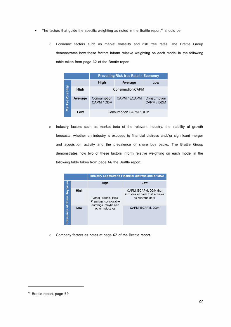
The factors that guide the specific weighting as noted in the Brattle report45 should be:
o Economic factors such as market volatility and risk free rates. The Brattle Group
demonstrates how these factors inform relative weighting on each model in the following
table taken from page 62 of the Brattle report.
o Industry factors such as market beta of the relevant industry, the stability of growth
forecasts, whether an industry is exposed to financial distress and/or significant merger
and acquisition activity and the prevalence of share buy backs. The Brattle Group
demonstrates how two of these factors inform relative weighting on each model in the
following table taken from page 66 the Brattle report.
o Company factors as notes at page 67 of the Brattle report.
45 Brattle report, page 59

28
Key concepts and terms
Conditions in the market for funds are such that a capital intensive business requiring a substantial volume
of debt would currently be unable to secure its entire requirement in Australian capital markets nor would it
be efficient to do so. It would be prudent for a large regulated utility to acquire debt from a number of
sources including international capital markets.
The domestic and international markets in which a large Australian regulated utility might expect to be able
to obtain funds at the lowest total costs are:
1. Australian domestic bond market;
2. Australian bank market;
3. US public bond (144a) market;
4. US private placement market;
5. Asian bank market;
6. Sterling market; and
7. Eurobond market.
It is generally accepted that the Sterling and Eurobond markets are likely to be difficult to access. In the
Sterling market, lenders generally finance issuers with credit ratings of BBB+ or above. In the Eurobond
market, the minimum issue size of €500 million is likely to be a barrier to an Australian service provider.
Funding costs in this market are generally higher than in comparable markets, and the minimum issue size
creates problems for Australian borrowers requiring cross currency swaps and future refinancing.
Question 5
Aside from a balance between debt and equity financing, are there other characteristics of the way in
which an efficiently financed entity would approach its financing task that should be considered in
estimating the allowed rate of return?

29
The Australian domestic bond market is less well developed than its counterparts in Europe and North
America, and a large Australian regulated utility seeking to access this market may have some difficulties
because issues are generally restricted to more highly rated enterprises. However, investors participating in
the bond market understand Australian utilities regulation, and market access negates any requirement for
cross currency hedging.
The principal source of Australian dollar debt finance for a large Australian regulated utility is the Australian
bank market. However, tenor is an issue in this market: it may be available for 5 to 7 years, but only a
small number of banks have the capacity to finance for as long as 7 years.
Longer term financing, with a tenor of around 10 years, is only available in highly liquid debt markets in the
United States, principally the public bond market (144a market), and the private placement market.
The benchmarking of service providers cannot occur in the abstract—they are dependent upon the reliability
of gas suppliers, the location of the assets, the conditions in which they are operated and maintained, the
state and efficiency of capital markets, the credit-worthiness of contractual counterparties and so on. These
are matters susceptible to subjective judgment, and these judgments are ones against which a final
determination of a return on capital that meets the requirements of the Rules as a whole must be made.
Question 6
Is it still appropriate to separate a conceptual benchmark from its practical implementation?
Question 7
Does the current definition [of benchmark efficient entity] reflect an appropriate level of detail for the
conceptual definition? Are there other factors which should be considered?

30
APIA submits that the benchmark efficient entity, in the context of the allowable rate of return objective,
cannot be applied in a “one size fits all” manner. This is evident from the words “with a similar degree of
risk which applies to the service provider”
In APIA’s view the regulator can only achieve this by considering what the service provider’s individual risk
characteristics would be, assuming the service provider met benchmark levels of efficiency. It cannot
undertake this task in the abstract, by simply having regard to generic risks that might be faced by some
conceptual; entity. This conclusion is also supported by the AEMC’s statement that:
“the objective is focused on the rate of return required by the benchmark efficient service provider, with
similar risk characteristics as the service provider the subject of discussion”46;
“the regulator must determine a rate of return that is consistent with that required by a benchmark efficient
firm with similar risk characteristics to the service provider in question”47; and
“the [allowable rate of return objective] incorporates the concept of a benchmark efficient service provider,
which means that the regulator can conclude that the risk characteristics of the benchmark efficient service
provider are not the same for all service providers across the electricity transmission, electricity distribution
and gas and / or within those sectors”48
It is also a point made by the Brattle Group in the Brattle Report. It argues that “[p]rovided that the range
has been developed in an appropriate way that takes account of the market and industry factors described
in this section, the final step is to consider the relative risk of the target company compared to the sample of
companies from which the cost of equity range has been developed. The cost of equity is adjusted
upwards or downwards depending on the target entity’s risk characteristics relative to those of the sample.
46 Rule determination page iii 47 Rule determination page 65 48 Rule determination page 67

31
It is APIA’s view that the concept of the benchmark efficient entity refers to gearing and other financial and
other financial parameters for a going concern. Therefore to answer the AER’s question, APIA’s does not
see how a prescriptive conceptual benchmark will help to achieve the allowable rate of return objective for
the reasons outlined above.
Again, APIA fails to see how stakeholders can agree to factors while it remains unclear what is being
measured. However, APIA suggests that there should be a preference for constructing samples that include
companies that are comparable to the service provider in question. To do otherwise would seem contrary to
achieving the allowable rate of return objective requiring the benchmark efficient entity with a similar degree
of risk.
APIA does support the use of a wider range of credit ratings and benchmark terms for debt than has been
used in the past and. appropriately also is seen to consider comparable companies with in similar credit
rating bands to assist in determinations of the cost of debt for individual service providers.
A process that could be used to determine risk levels for service providers is:
1. Define the risks for a service provider.
2. Identify whether they are systematic or non-systematic.
3. Examine the risks of the peers of the service provider.
4. Assess the relevance of the risk for benchmarking.
Question 8
In relation to the current definition of the conceptual benchmark, is more or less detail preferable?
Question 9
Are the proposed factors reasonable?

32
Gas transmission pipelines are substantially different from electricity networks. A full discussion of these
differences in provided at Schedule 3.
Yes. There are characteristics that differentiate the level of risk in gas and electricity sectors. Further, each
gas transmission asset has unique characteristics that differentiate the level of risk between gas
transmission assets. APIA’s view on these characteristics is presented in detail at Schedule 3.
A summary of the differences between some major regulated gas transmission pipelines is:
Pipeline Primary customer base Source of gas Revenue Model
DPNGP Minerals processing
Power generation
Manufacturing
Offshore Carnarvon
basin – NWSG
and Varanus
Island Export
competition
Contract Carriage
GGP Mining Offshore Carnarvon
Basin ‐NWSG and Varanus Island
Contract Carriage
AGP Power Generation Single offshore field –
Blacktip
Formerly Amadeus
Basin
Contract Carriage
Question 10
Are there other factors which should be considered?
Question 11
Are there characteristics that differentiate the level of risk in the gas and electricity sectors, or between
distribution and transmission networks?

33
RBP Power Generation
Large Industrial
Residential &
Commercial
Surat‐Bowen Basin
Conventional and
increasingly coal
seam gas
Contract Carriage
VTS Residential &
Commercial
Small‐mid industrial;
Multiple offshore
basins
Linkages to
QLD/SA supply
through NSW
Storage facilities
Market Carriage
The characteristics to take into account have to be determined for each service provider at the time of
determination. As mentioned above, a process to do this could be:
1. Define the risks for a service provider.
2. Identify whether they are systematic or non-systematic.
3. Examine the risks of the peers of the service provider.
4. Assess the relevance of the risk for benchmarking.
APIA is of the clear view that the specific risks of a firm must be taken into account. It is our reading of the
NGR that this is required.
Section IV Part D of the attached Brattle Report at Schedule 2 covers characteristics that should, and have,
been taken into account when assessing the level of risk.
Question 12
Are there other characteristics that should be taken into account when assessing the level of risk?

34
APIA believes these differences can be estimated to a sufficient extent for gas transmission pipelines that
they must be.
For electricity transmission and distribution and gas distribution it is more likely that the similarities outweigh
the differences.
APIA commends to the AER Section IV Part D of the attached Brattle Report at Schedule 2 which deals
specifically with the issue of risk positioning.
Overall rate of return
It is important that the regulator have full regard to all relevant evidence and this could include a top down
approach. However, there are significant problems with obtaining top down WACC estimates, both in terms
of relevance and quality. The examples cited in the Issues Paper are excellent examples of top down
estimates that that have at best limited relevance and can be low quality.
Each of the methods identified are problematic, in terms of relevance and/or in terms of the quality. It is
worthwhile reviewing the issues of relevance and reliability/quality for each of the methods identified in the
Issues Paper:
1. Brokers’ reports: The relevance of brokers’ reports is doubtful, but should not be excluded. Broker
reports should be considered in the context that the brokers provide recommendations to hold, buy or
sell for the purposes of advising clients that generally have a portfolio of stocks and are looking at the
Question 13
To the extent that different risk levels exist, can these differences be estimated in a manner consistent
with the regulatory principles outlined in section 2?
Question 14
To date our practice has been to estimate the allowed rate of return based on the standard WACC
formula. Should we continue with this, or if not, what alternative approaches should be explored?

35
issues of asset allocation. That is, investors have a certain amount of capital available and seek to
optimise their returns by allocating their capital in a way that is designed to give them the best risk-
weighted return. Thus analyst estimates are focussed on the relative value of a stock rather that their
absolute value. APIA refers to Brattle’s consideration of other evidence at Section III.F.5 of its report.
2. Trading multiples: In its Report to APIA Brattle49 identifies a number of “conceptual problems with this
approach, so that it has no value as a cross check against the regulator’s cost of capital determination.
Brattle identifies two main assumptions that render this approach of no value: (i) the company to which
the approach is applied is likely not to consist entirely of a regulated business and (ii) that the
regulator’s cost of capital determination is the only factor impacting the market value of the stock.
Further to this advice, the effect of market cycles and volatility must be properly considered. Depending
where the market is in it’s cycle – “bear” or “bull” a regulated utility stock may appear undervalued or
overvalued relative to its regulatory value. Market volatility must also be properly considered. In sum,
trading multiples can neither be considered as having much relevance or quality as top down estimates
of the WACC.
3. Financibility tests: These tests were developed by IPART, not to determine the rate of return, but to
assess whether the revenue allowances in its determinations would undermine the financial viability and
financibility of regulated businesses. That is, it wanted to make sure that regulatory outcomes would
not jeopardise the viability of the business or have the effect of increasing, inadvertently the cost of debt
through reduced credit ratings. The intent of such an approach is laudable, but the modelling approach
designed to reflect the way credit ratings agencies determine credit ratings is problematic, given (i) that
credit ratings agencies do more than mechanical modelling exercises and (ii) such approaches say
nothing about the cost of debt and equity. Consequently, such tests are not relevant and, even if they
were are not reliable, even in attempting to achieve the goal of determining the impact of a regulatory
decision on credit ratings.
4. Estimates of other regulators: This method is clearly fraught in terms of relevance and
reliability/quality. Regulators’ decisions are made at a time and for a particular asset. Therefore they
are relevant to that time and asset and not to another. Moreover, if regulators were to base rate of
49 Estimating the Cost of Equity for Regulated Companies, The Brattle Group, February 2013, pages 37,38

36
return decisions either on their own previous decisions or another regulator’s decisions they will suffer
the problem of regulatory group think. It is essential that regulators start afresh each time they
undertake a review of the Rate of Return to properly consider the question: what is the rate of return
that meets the ARORO for this business at this point in time?
On top of all of this, if any of these methods were to be used as part of developing a top down estimate it
would then be necessary to convert them (with appropriate weightings) into a cost of equity and a cost of
debt in a manner that is consistent with the Rules. Significantly, the WACC implied by any of most of these
is a post- tax WACC. In the case of analyst views the post-tax WACC that imputation credits are not
valued by investors. In the case of trading multiples the treatment value of tax credits are unknown;
however, if analysts’ recommendations are considered as influential on investors then these effectively do
not include any value for tax credits. Between the treatment of tax credits and the difficulties of taking a
post- tax WACC and converting it into a vanilla WACC further broken down in to costs of equity and costs
of debt with their respective weights, it is difficult to see how the requirements of the Rules could be met
(especially the cost of debt provisions or Rule 87) – at least in practical sense – using such an approach.
Overall rate of return considerations are best dealt with by considering all relevant evidence estimating the
cost of equity and the cost of debt and how they inform each other in determining a rate of return that will
achieve the ARORO. This could include benchmarks and test as discussed in Question 14. However, as
demonstrated the currently identified methods are unlikely to be very informative in assessing the rate of
return.
Rather, it is more likely that looking at overall rate of return considerations will be best achieved by
considering the various models for estimating the cost of equity and the cost of debt and how they inform
each other in determining a rate of return that will best achieve the ARORO.
Question 15
How can overall rate of return considerations be used under the new rule framework? This may include
consideration of the relevance of the methodologies identified above (or others not yet identified), and
how such information could be used.

37
Return on equity
No, see APIA comments on the AER proposed principles above. The discussion in Section 3.1 covers
principles to be applied in reasoning.
It is clear from the AEMC’s reasoning that a methodology that considers relevant models, techniques,
evidence and data is utilised is more likely to achieve the allowed rate of return objective. APIA believes an
appropriate methodology to do this has been articulated as APIA’s first proposal on page 17 of this
submission.
APIA notes the methodology outlined above requires significant regulatory discretion and judgement. APIA
must emphasise that the regulators discretion and judgement must be applied in a rigorous and transparent
manner, clearly detailed in decision documents and grounded in NGO, RPPs and Rule 87.
The advantages of such an approach are:
It delivers a reliable rate of return that avoids the false precision of single model.
The use of multiple models means the effects of biases and weakness of any single model are
reduced.
The consequences of discretionary decisions required in estimating the rate of return of a single
model (or any errors that occur) are muted as the influence of any one model is not too great.
Question 16
Are the assessment criteria presented in section 3.1 an appropriate basis for evaluating the cost of
equity methodology in order to meet the allowed rate of return objective?
Question 17
What overall cost of equity methodology best meets the allowed rate of return objective?

38
If the guidelines effectively establish the principles and articulate the criteria under which the
regulator will make decisions it will result it transparent, logical and clear use of regulatory
discretion.
It maximises stability over time by minimising the effect of instability in any single model.
APIA recognises this will be an aspect in the determination process requiring understanding and thoughtful
reasoning and because of this has started to articulate a framework for this judgement to be applied within,
largely outlined by the Brattle report. APIA considers this is an area that will require further work and looks
forward to working cooperatively with the AER and other stakeholders in establishing a clear framework for
use by the regulator so that it not seen to be applying it regulatory judgement in isolation.
In summary, APIA is firmly of the view that no individual cost of equity model can meet the allowable rate of
return objective.
The attached report from The Brattle Group and the covering note by Professor Stewart Meyers are
unequivocal on this point:50
It is useful to recognize explicitly at the outset that models are imperfect. All are simplifications of reality,
and this is especially true of financial models. Simplification, however, is also what makes them useful. By
filtering out various complexities, a model can illuminate the underlying relationships and structures that are
otherwise obscured. After all, while a perfect scale model representation of the city might be highly
accurate, it would make a poor road map. It is therefore imperative that regulators and other users of the
models use sound judgment when implementing and using the models - - there is no one model or set of
models that are perfect.
50 Brattle Group report p8.
Question 18
What individual cost of equity model best meets the allowed rate of return objective?

39
The gap between financial models and reality can sometimes be quite significant (as was painfully
demonstrated by the recent financial crisis). There is no single, widely accepted, best pricing model to
estimate the cost of capital – just as there is still no consensus on some fundamental issues, such as the
degree to which markets are efficient. Analysts have a host of potential models at their disposal, and it
must be acknowledged that cost of capital estimation continues to be part art. Several regulators as well as
textbooks therefore recommend that the “best practice” is to look at a totality of information from alternative
methodologies. 51
Academics, practitioners and regulators have all acknowledged that there is no one way to determine the
cost of equity. In the academic literature, several prominent researchers have commented that the use of
more than one method is important. For example, Professor Myers of the Massachusetts Institute of
Technology commented:
Use more than one model when you can. Because estimating the opportunity cost of capital is difficult, only
a fool throws away useful information. That means you should not use any one model or measure
mechanically or exclusively. Beta is helpful as one tool in a kit, to be used in parallel with DCF models or
other techniques for interpreting capital market data.52
Professors Berk and DeMarzo of Stanford University in their corporate finance textbook comment on the use
of the CAPM, DDM, and other models by practitioners, and state:
In short, there is no clear answer to the question of which technique is used to measure risk in practice — it
very much depends on the organization and the sector. It is not difficult to see why there is so little
consensus in practice about which technique to use. All the techniques we covered are imprecise.
Financial economics has not yet reached the point where we can provide a theory of expected returns that
gives a precise estimate of the cost of capital. Consider, too, that all techniques are not equally simple to
51 See, for example, the Ontario Energy Board’s EB-2009-084 decision, December 2009, the U.S. Surface Transportation Board’s Ex. Parte 664 (Sub-No. 1) decision, January 2009, and Roger A. Morin, New Regulatory Finance, Public Utilities Report Inc., 2006, Chapter 15. 52 Stewart C. Myers, “On the Use of Modern Portfolio Theory in Public Utility Rate Cases: Comment,” Financial Management, Autumn 1978.

40
implement. Because the trade-off between simplicity and precision varies across sectors, practitioners
apply the technique that best suit their particular circumstances.53
Similarly, Roger A. Morin, in the context of U.S. regulation, mentions the use of the CAPM, DDM, risk
premium models, and the comparable earnings method, concluding:
No one individual method provides the necessary level of precision for determining a fair return, but each
method provides useful evidence to facilitate the exercise of an informed judgment. Reliance on any single
method or pre-set formula is inappropriate when dealing with investor expectations because of possible
measurement difficulties and vagaries in individual companies’ market data.54
Regarding the methods used to determine the so-called Equity Risk Premium (ERP), the Ontario Energy
Board concluded:
the use of multiple tests to directly and indirectly estimate the ERP is a superior approach to informing its
judgment than reliance on a single methodology.55
Critically, APIA is of the view that each methodology applied to assist in determining the cost of equity must
be applied fully and faithfully. In particular, for each model to which the AER has regard, the results of that
model must be determined with the degree of rigour as if it were the sole model being relied upon to guide
the regulator’s discretion. It would not be appropriate for the AER to purport to have had regard to a model
or methodology which has been applied half-heartedly.
53 Jonathan Berk and Peter DeMarzo, Corporate Finance: The Core, 2009, (Berk & DeMarzo 2009) p. 420. 54 Roger A. Morin, New Regulatory Finance, Public Utilities Reports, Inc., 2006, (Morin 2006) p. 428. Quoted in Brattle Group p48. 55 Ontario Energy Board, “EB-2009-0084, Report of the Board on the Cost of Capital for Ontario’s Regulated Utilities,” Issued December 11, 2009, p. 36 (emphasis in the original). Quoted in Brattle Group p49.

41
APIA notes that the Rules require the AER to have regard to “relevant estimation methods, financial models,
market data and other evidence”.56 APIA considers, and its consultations with the AEMC confirm, that
“relevant” is intended to be a very low threshold. It therefore reflects a presumption that a broader range of
models, methods and evidence are more likely to be “relevant” than not.
Within the context of the Rules, APIA considers that the threshold question is not “what other evidence is
relevant” as much as “is there any evidence that could reasonably be considered to be irrelevant?”
In this regard, APIA has asked The Brattle Group to assess two approaches previously applied by the AER,
being an assessment of premiums paid in takeover transactions and an assessment of market-to-RAB
multiples.57 In both cases The Brattle Group has found that these methodologies are of low relevance in
informing the regulator’s view on a business’ required cost of capital.
Consistent with its broader views on this matter, APIA considers that it is incumbent on the AER to:
include a broad range of models, market information and data sources in the Guideline, consistent
with the “relevant” threshold, and
have regard to further information proposed by the regulated business in the context of a regulatory
price review submission (i.e. information or data sources not already reflected in the Guideline)
through the lens of the “relevant” threshold.
56 Rule 87(5)(a). 57 Brattle Report page 58.
Question 19
What other evidence (estimation methods, financial models, market data and other estimates) is
relevant to the determination of the cost of equity?
42
In summary, APIA submits that evidence or information should not be discarded lightly. The advice to APIA
from the Brattle Group is that the following methods are relevant to determining the cost of equity:
Sharpe-Lintner CAPM
Empirical CAPM
Consumption-based CAPM
Fama-French Three-factor Model
Arbitrage Pricing Theory (Black CAPM)
Dividend Discount Model (both single-stage and multi-stage)
Residual Income Model
Risk Premium Approaches
Build-up Method
Comparable Earnings
Methods that the Brattle Group do not consider relevant are:
Market-to-book and Earnings Multiples
Analyst Reports
Return on debt
In summary, APIA considers that the presentation of this question is overly simplified, and has scope to
truncate the debate in a way that is not in accordance with the Rules.
Question 20
What are the advantages and disadvantages of portfolio approaches compared with the current "on the
day" approach to the return on debt?
43
Rule 89(10) clearly does not provide an “either/or” approach as suggested by the question, but that either
option (or indeed a combination of them) is acceptable. Moreover, the term “without limitation” in Rule
87(10) clearly indicates that some other methodology would be equally acceptable:
(10) Subject to subrule (8), the methodology adopted to estimate the return on debt may, without
limitation, be designed to result in the return on debt reflecting:
(a) the return that would be required by debt investors in a benchmark efficient entity if it raised
debt at the time or shortly before the time when the AER's decision on the access arrangement for
that access arrangement period is made;
(b) the average return that would have been required by debt investors in a benchmark efficient
entity if it raised debt over an historical period prior to the commencement of a regulatory year in
the access arrangement period; [the “moving average” approach] or
(c) some combination of the returns referred to in subrules (a) and (b).
APIA considers that is inappropriate (indeed beyond powers) for an AER Guideline to truncate alternate
approaches and methodologies that are explicitly allowed in the Rules, and to restrict consideration of other
methodologies that are envisioned (albeit not specified) as potentially becoming available in the future.
APIA considers that the Rules attempt to reflect the diversity of approaches that different businesses take to
managing their debt portfolios. In this regard, APIA considers that it is not reasonable to espouse a “one
size fits all” approach – in order to avoid arbitrarily advantaging or disadvantaging the regulated business,
the approach to estimating the efficient regulatory cost of debt must reflect the business’ debt management
practices.
In this regard, APIA is firmly of the view that the decision about which methodology to apply (that is, Rule
87(10)(a) or (b)) or the extent to which they are combined under 87(10)(c), or indeed whether some
other methodology should apply, should be at the discretion of the service provider. Critically, APIA is
concerned that the AER would purport to put itself in a more expert position on the management of a
business’ debt portfolio than the management of the business.

44
APIA considers that there is significant work to be done on the cost of debt component of the Guideline,
and this work should reasonably be undertaken once the higher level direction has been decided. In
particular, matters surrounding sources of bond yield information or the composition of any benchmark bond
portfolio are important matters which will require careful consideration.
APIA looks forward to working with the AER on these matters of detail.

ESTIMATING THE COST OF EQUITY: INTRODUCTION AND OVERVIEW
Stewart C. Myers
February 17, 2013
1. Introduction
The Australian Pipeline Industry Association (APIA) has requested me to review the
methods and evidence that Australian energy regulators should take account of when
determining the cost of equity for energy infrastructure companies. The request followed the
Australian Energy Market Commission’s new Rule 87 and its new “allowed rate of return
objective.” The new Rule requires in part that “regard must be had to relevant estimation
methods, financial models, market data and other evidence” in determining the overall rate of
return and that “regard must be had to the prevailing conditions in the market for equity funds”
in determining the cost of equity capital.1
This report accompanies a more extensive and detailed report by colleagues at The
Brattle Group, Inc. (Brattle Report).2 That report reviews models and methods that have been
used for determining the cost of equity. I comment broadly on several of these models, including
the Sharpe-Lintner Capital Asset Pricing Model (CAPM), the three-factor Fama-French model
and the single- and multi-stage dividend discount models. I consider whether regulators should
weigh estimates from two or more models, or whether it is better to rely exclusively on one
model, for example the CAPM. I discuss how prevailing market conditions could be taken into
account. For example, how should the extremely low interest rates prevailing now in most
developed economies affect estimates of the cost of equity?
My comments reflect the current state of finance theory and research and my experience
in using that theory in practice. Much of my practical experience has focused on valuation and
estimation of the cost of capital, in both regulated and non-regulated settings.
1 Australian Energy Market Commission, AEMC Final Position Rules: Amendments to the Natural Gas
Rules, 15 November 2012, Rule 87 (5a), (7). 2 The Brattle Group, Inc., Estimating the Cost of Equity for Regulated Companies, prepared for the
Australian Pipeline Industry Association, February 17, 2013. I am a principal of The Brattle Group, but did not contribute to the Brattle report.

2
Sections 2, 3 and 4 of this report focus on three models for estimating the cost of equity:
the CAPM, the Fama-French model and dividend-discount models. Section 5 briefly discusses
size premiums and the “build-up” method. Section 6 discusses possible responses to “prevailing
market conditions.” Section 7 sums up my conclusions and recommendations.
The Brattle Report describes and evaluates the CAPM and other models much more
extensively than here. This report is an introduction and overview based on my professional
knowledge and experience.
2. The Capital Asset Pricing Model (CAPM)
Cost of Equity = Risk-free interest rate + beta × Expected equity risk premium
“All economic models are wrong, but some are useful.” The CAPM is of course wrong,
that is, imperfect and incomplete, but it has many advantages. It the model most widely used by
U.S. corporations to estimate the cost of capital.3
Advantages of the CAPM. The CAPM is simple and logical. It respects the key
distinction between market risk, which all stock-market investors bear, and unsystematic, firm-
specific risks, which “wash out” of diversified portfolios and should not affect the cost of equity.
Stock markets in developed economies are dominated by diversified investors.
The CAPM requires three inputs: the risk-free rate of interest, the risk measure beta and
the expected equity risk premium (also known as the market risk premium). These inputs can be
estimated with tolerable accuracy. The risk-free rate of interest can be observed from rates on
government bills, notes or bonds, depending on maturity. Beta can be estimated from past rates
of return for individual stocks and for the stock market as a whole.4
Companies in industries that appear low-risk, including most regulated industries,
generally have below-average betas, that is, betas less than one. Younger growth companies
3 See J. R. Graham and C. Harvey (2001), “The theory and practice of corporate finance: Evidence from the
field,” Journal of Financial Economics 60, 187-243, and J. R. Graham and C. Harvey (2002), “How do CFOs make capital budgeting and capital structure decisions?” Journal of Applied Corporate Finance 15, 8-23.
4 Accuracy is better if betas are estimated for portfolios rather than individual stocks. Suppose the object is to measure the average beta of a sample of comparable companies. The best procedure is to first form a portfolio of the companies’ stocks, then estimate beta from returns on the portfolio. The portfolio beta is more reliable than an average of betas for the individual stocks.

3
generally have high betas. Thus betas line up with intuitive views of risk, which increases
confidence in CAPM estimates of the cost of equity.
The expected equity risk premium is difficult to forecast directly, but there is long-term
historical evidence on average equity risk premiums in most developed economies.5 6 We know
what normal risk premiums have been.
There is always room for argument, but careful applications of the CAPM tend to give
estimates of the cost of equity that are sensible and reasonably stable over time. Nevertheless the
CAPM does not give conclusive answers. Use of the CAPM should not exclude other models.
The reasons are as follows.
Four reasons for caution. First, the CAPM, like other models for estimating the cost
of equity, does not generate a single estimate of the cost of equity, but a range. Betas and equity
risk premiums are statistical estimates, which are exposed to statistical noise and potential error.
For example, a typical confidence limit for an estimated industry beta (plus or minus two
standard errors) could be ±.2 – a beta estimated at .8 could actually lie between .6 and 1.0.7
Suppose that the risk-free rate is 5% and the estimated equity risk premium is 6%. The
confidence limit for the cost of equity would span a range from 5 + .6×6 = 8.6% to 5 + 1.0×6 =
11%. The range is wider if uncertainty about the true equity risk premium is introduced.
Of course CAPM analyses must zero in on a specific number for the cost of equity. It is
important to remember, however, that the number is drawn from a range.
Second, empirical estimates of the security market line are “flatter” than the CAPM
predicts. (The security market line is the relationship between beta and expected rate of return.)
That is, average returns for the lowest-beta stocks have been higher than the CAPM predicts.
Average returns for the highest-beta stocks have been lower. Thus CAPM cannot be a complete
model of risk and return in financial markets.
5 Average risk premiums from 1900-2011 are available for 22 developed countries. See Credit Suisse
Global Investment Returns Sourcebook 2012, Credit Suisse Research Institute, February 2012. 6 Arithmetic averages should be used when the cost of equity is based on historical risk premiums.
Sometimes geometric averages are proposed, which is a mistake. There are some statistical issues that could impart an upward bias to arithmetic-average premiums and
could justify placing some weight on geometric averages. Jacquier, Kane and Marcus derive adjustments to remove the bias, but the adjustments are small when cash flows are forecasted for, say, five or ten years. See E. Jacquier, A. Kane and A. Marcus (2005), “Optimal Estimation of the Risk Premium for the Long Run and Asset Allocation: A Case of Compounded Estimation Risk,” Journal of Financial Econometrics 3, 37-55.
7 This example assumes a single regression estimate. An analyst could look to other information, for example, “rolling betas” estimated over much longer periods. On the other hand, confidence limits widen when predicting future betas (out of sample).

4
The “empirical CAPM” has been proposed for estimating the cost of equity. In this
approach, the cost of equity is derived from the empirical security market line, that is, from the
long-run average relationship between beta and expected return. The CAPM says that the
intercept of the security market line (at beta = 0) should be the risk-free interest rate. The
empirical CAPM uses a higher intercept (call it the SML intercept) because the empirical
security market line is flatter. The equation for the cost of equity is:
Cost of Equity = SML intercept + beta × (Expected market return - SML intercept)
The empirical CAPM is rarely used by non-regulated firms, although I understand it has
been given weight in some regulatory settings. This model is nevertheless an important reminder
for analysts and decision-makers. The CAPM has not been randomly wrong; it has
systematically understated long-run average returns on low-beta stocks. Stocks of regulated
firms are almost always low-beta, that is, less than 1.0.
Third, the CAPM assumes that investors’ portfolios are fully diversified and therefore
highly correlated with returns on the market portfolio, that is, the entire stock market. Therefore
the market portfolio cannot be defined as a limited slice of the entire market. For example, a
U.S. application of the CAPM could not define the market portfolio as the Massachusetts stock
market, because no diversified investor would invest only in Massachusetts companies. Usually
the U.S. market portfolio is defined as the S&P 500 Index or some still broader index.8
The case for the CAPM becomes less convincing when it is applied in smaller
economies, especially economies with no barriers to the inflow or outflow of capital from or to
international markets. Thus analysts in countries such as Canada, New Zealand and Australia
should not focus exclusively on betas estimated with local stock-market indexes. For example,
Canadian regulators consider betas for the U.S. as well as the Canadian market.9
It makes sense to check betas estimated against broader indexes, or to check whether
local betas match betas for similar companies in other countries. Suppose, for example, that an
Australian regulator estimates betas for a portfolio of local electric utilities. It is then useful to
check the estimates against betas for similar electric utilities in other countries.
8 Even U.S. indexes may be too narrow. For example, I have considered betas measured against a world
stock-market index in valuing an oil field that produces for the world market. 9 See Brattle Report, Section IV.A.

5
Fourth, a mechanical application of the CAPM may be dangerous in current market
conditions. Central banks have forced interest rates down to exceptionally low levels. The
“flight to quality” by investors during the recent financial crisis has also pushed down interest
rates on government debt and high-quality corporate debt. Routine CAPM estimates of costs of
equity are therefore much lower than past estimates, and much lower than “normal” equity rates
of return. In some cases, routine implementations of the CAPM have yielded costs of equity less
than the regulated company’s cost of debt – an impossible result.10
Routine applications of the CAPM assume that the equity risk premium is stable. But the
premium fluctuates. It clearly increased because of the flight to quality during the financial
crisis. It is probably still abnormally high. For example, the average equity risk premium in
Graham and Harvey’s latest survey of U.S. financial executives has increased to levels last
observed in the financial crisis in 2009.11
The equity risk premium compensates investors for absorbing the volatility of the market
portfolio and also for the poorer liquidity of equities compared to government debt securities.
Investors pay “liquidity premiums” for government debt and therefore accept lower interest
rates. The liquidity premium increased during the financial crisis; very low government interest
rates suggest that it is still high. Thus the expected equity risk premium is probably still above
normal levels.
I present these four issues not to argue against the CAPM, but to argue against its
exclusive use when other methods are feasible.
3. The Fama-French three-factor model
Cost of Equity = Risk-free interest rate + beta × Expected equity risk premium
+ bsize × Expected return on size factor
+ bvalue × Expected return on value factor
10 See Brattle Report, Section II.B. 11 J. R. Graham and C. R. Harvey (2013), “The Equity Risk Premium in 2012,” Duke University, SSRN
2206538, Table 1. Average premiums from the Graham-Harvey survey peaked at 4.74% in the second quarter of 2009, fell below 3% in 2010, and increased to 4.48% by the second quarter of 2012, the last date in the survey. I believe these premiums are unrealistically low, but the time pattern is worth noting.

6
The Fama-French model is an example of arbitrage pricing theory (APT). The model
captures the excess average returns earned by investors in small stocks and in value stocks. The
“size” factor is the difference between the expected rates of return on the smallest and the largest
stocks, where size is measured by market capitalization. The “value” factor is the difference
between the expected rates of return on value vs. growth stocks. Value stocks are stocks with
high ratios of book value to market value per share. Growth stocks sell at high market-to-book
ratios and therefore low book-to-market ratios.
Fama and French showed that both the size and value factors generate significant positive
rates of return on average. If the CAPM were strictly correct, the expected rate of return on both
of these factors would be zero.
The Fama-French model says that a company’s cost of equity depends on not only on
beta and the equity risk premium, but also on its exposures to the risks of small-cap stocks (vs.
large-cap stocks) and the risks of value stocks (vs. growth stocks). The exposures to these size
and growth factors are measured by bsize and bvalue, which are in effect two additional betas.
The Fama-French model in practice. The Fama-French model is superior to the
CAPM for many purposes. It explains past returns on large portfolios of common stocks much
better than the CAPM. It is widely used in practice to test for superior performance of actively
managed portfolios. For example, any thorough analysis of the performance of pension or
mutual funds now corrects for the funds’ exposures to the Fama-French factors.12
The Fama-French model is an extremely important contribution to understanding risk and
return. It is used in practice for many important tasks, but not to estimate the cost of equity.
Attempts to use the model for that task typically encounter three chief difficulties.
First, the factor exposures bsize and bvalue are (in my experience) unstable when estimated
for individual stocks or portfolios of stocks in narrowly defined industries. They “bounce
around” more than the CAPM beta.
Second, it is difficult to understand why the factor exposures bounce around for
companies or industries when business risks appear stable. It is not easy to see what risks the
factor exposures are measuring. Thus estimates of bsize and bvalue generally get less intuitive
support than estimates of beta.
12 Such evaluations of investment performance can use past returns for the investment portfolio and for the
size and value factors. There is no need to estimate expected returns on the size and value factors.

7
Third, the expected risk premiums for the size and value factors are difficult to forecast.
Of course the CAPM’s equity risk premium is also difficult to forecast, but more historical data
are available, and there has been at least a partial convergence of views about the equity risk
premium.
There is no need for financial analysts or decision-makers to lock out the Fama-French
model as a method for estimating the cost of equity. Research may clear the way for more robust
estimates from the model or from extensions of it.
4. Dividend discount models
Dividend discount models start with the valuation principle that stock price equals the
discounted present value of expected future cash payouts to the stockholder. This principle
should hold for all companies, but it is only useful for companies that are mature, consistently
profitable and reasonably stable.
The valuation principle implies that an analyst should be able to (1) observe stock price,
(2) forecast cash payouts and (3) back out the discount rate that explains the stock price. The
discount rate is the expected rate of return to the stockholder and therefore the cost of equity.
Dividend discount models are hard to apply generally. They are rarely used for growth
companies or in industries where business risks come and go, product prices are volatile, and
markets and technologies are changing. But the models do make sense for many regulated firms,
providing that the firms make regular cash payouts to shareholders.
Constant-growth models. Suppose one could find a mature company that will grow at
a constant expected rate g for the indefinite future. If the payout ratio is constant and dividends
per share grow at g, the discount rate that explains stock price is:
Discount rate = cost of equity = DIV1/P0 + g,
where DIV1 is next period’s dividend (at date 1) and P0 is the current price (at date 0).
This formula makes the stringent assumption that the expected rate of growth is constant
in perpetuity, or at least for the indefinite future. Few companies meet this assumption. Even if
one could find such a company, forecasts of growth in the very long run would not be available.
For example, forecasts by security analysts of “long-run” growth in earnings extend to five years
at most.

8
The constant-growth model overestimates the cost of equity when near-term growth
cannot be sustained. For example, the U.S. Surface Transportation Board (STB) once used the
constant-growth model to track the cost of equity for U.S. railroads. But by 2005 the largest
railroads were expanding rapidly and profitability was increasing. Security analysts were
forecasting “long-run” earnings growth for some railroads at 15% per year. Such growth could
not be sustained, so the constant-growth model overstated the true cost of equity by a wide
margin. The STB therefore changed over to a blend of the CAPM and a multi-stage dividend
discount model.13
Multi-stage models. Multi-stage models improve dividend forecasts by distinguishing
near-term and long-term growth. 14 For example, colleagues at the Brattle Group use security
analysts’ forecasts for the first five years of earnings and dividends, but then assume that growth
converges over ten years to the long-term growth rate of GDP. Thus there are three stages:
initial growth for five years, convergence over ten years, and perpetual growth thereafter. Future
cash flows in all three stages are then discounted to present value. The discount rate that
explains the stock price is the cost of equity.
The Ibbotson SBBI Yearbooks implement a similar three-stage model,15 as does
Bloomberg.
Multi-stage dividend discount models can be a valid method for estimating the cost of
equity. They often work well for regulated industries, which are more likely to be populated
with companies that are mature, reasonably stable and paying out cash to investors.
The multi-stage models focus on cash returns to investors. This is an important
advantage. If the cash returns are unbiased forecasts, then the model must yield the expected rate
of return to investors. The analyst does not have to measure risk and expected risk premiums.
The analyst does not have to assume an equilibrium model of risk and return, for example the
CAPM. The analyst looks directly at the cash payoffs that an investor can expect to receive.
Costs of equity derived from multi-stage dividend discount models are particularly useful
now. With extremely low current interest rates, routine applications of the CAPM, which use
“normal” equity risk premiums, can now yield cost of equity estimates that seem unreasonably
low. 13 See Brattle Report, Sections III.E and IV.C. 14 “Residual income models” are another form of multi-stage dividend-discount models. See Brattle Report,
Section III.E. 15 Ibbotson SBBI 2012 Valuation Yearbook, Morningstar, Chicago.

9
It is hard to measure year-to-year changes in the equity risk premium, but it is
nevertheless plausible to say that the premium currently remains at abnormally high levels.
Direct estimates of expected returns to investors, which the multi-stage dividend discount model
can provide, can test whether this plausible statement is in fact true. The difference between the
cost of equity from the dividend discount model and the risk-free interest rate is a direct estimate
of an expected risk premium demanded by investors. The expected market equity risk premium
can be backed out of this estimate.16
Notice that an analyst or decision-maker concerned with Industry X does not have to
perform this test on that industry. Suppose that the multi-stage dividend discount model is not a
good fit to Industry X but is a good fit to Industry Y. If application of the model to Industry Y
indicates a higher-than-normal equity risk premium, then the same higher-than-normal premium
should also apply to Industry X.
Three reasons for caution. Multi-stage dividend discount models can give robust and
credible estimates of the cost of equity, but there are three main reasons for caution. First, the
models are unreliable for companies facing volatile markets and changing technologies and for
growth companies that do not generate reliably positive free cash flow and make regular cash
distributions to investors. Second, the “long-run” growth rates estimated by security analysts
look out five years at most. These growth estimates may be noisy and biased. Third, the growth
forecasts are normally for earnings and dividends per share, and the number of shares
outstanding depends on share repurchases. There is a solution to the third problem, however.
Dividends and repurchases. Stock repurchases now constitute “the dominant form of
payout,” at least in the U.S.17 Repurchases complicate use of dividend discount models, because
repurchases change the number of shares outstanding and therefore the growth rate of dividends
per share. Therefore repurchases should be adjusted for when implementing dividend discount
models. But repurchases fluctuate and are hard to predict.
This problem has a simple solution, which I recommend going forward.18 Forecast
aggregate payout, dividends plus repurchases, to all shareholders. Calculate the discount rate
16 A beta estimate is required. The dividend discount model estimates the cost of equity directly. Given the
beta and the risk free rate, one can solve for the market risk premium that explains the direct estimate. 17 D. J. Skinner (2008), “The evolving relation between earnings, dividends and stock repurchases,” Journal
of Financial Economics 87, p. 584. 18 This revised method is explained in R. A. Brealey, S. C. Myers and F. Allen (2013), Principles of
Corporate Finance, 11th Ed., McGraw-Hill Irwin, Ch. 16.

10
that explains the company’s market capitalization, that is, the aggregate market value of all
shares outstanding at the current price P0. This discount rate is the cost of equity. The method
could be labeled an aggregate cash payout discount model.
The valuation principle is unchanged: stock price equals the discounted present value of
expected future cash payouts. But cash payouts include repurchases as well as cash dividends.
By forecasting total payout to all shareholders, one forecasts the sum of repurchases and
dividends, and avoids the challenges of forecasting repurchases and changes in the number of
shares outstanding.
I understand that Australian natural-gas pipelines rarely repurchase shares in significant
amounts. Nevertheless, the aggregate cash flow discount model is no more difficult to apply
than the traditional dividend discount model and is simpler and more robust generally.
5. The build-up method
Other models sometimes used to estimate the cost of equity are less well grounded in
theory and not as extensively tested as the models covered above. The other models may,
however, allow the analyst or decision-maker to introduce additional information and to apply
judgment in determining the final estimate.
The “build-up” method calculates the cost of equity as:
Cost of Equity = Risk-free rate + Equity risk premium + Size premium + Industry premium
The first two terms of the build-up cost of equity match the CAPM cost of equity if beta equals
1.0. If the size premium is zero and the industry premium equals (beta – 1) × Equity risk
premium, then the build-up method and the CAPM give identical answers.
The build-up method gives the analyst or decision-maker two additional degrees of
freedom, the industry premium and the size premium. The additional degrees of freedom are
probably the method’s main attraction.

11
Size premium. The Fama-French model can be invoked to justify addition of a size
premium to the cost of capital for small companies.19 Fama and French showed that investors in
small-cap stocks have earned above-average returns, after adjusting for the stocks’ above-
average betas.
The Fama-French model does not say that investors demand higher expected returns from
small-cap companies just because they are small. Higher expected returns come from bsize, the
exposure to the size factor, and the expected risk premium on the size factor, which proxies for
some underlying economic risk that small companies are especially exposed to.
The right question – if one accepts the Fama-French model – is not whether a company is
small or large, but whether the company’s exposure bsize is materially greater than zero. 20 Some
small-cap companies have negative exposure (bsize < 0); they act like large companies with
respect to the size factor. Some large companies have positive exposure (bsize > 0). Analysts
should not add size premiums without first estimating bsize for the company at hand or for a
portfolio of similar companies in the same industry.
Industry premium. The industry risk premium could be estimated by multiplying the
equity risk premium by the difference between the industry beta and 1.0. In this case the sum of
the industry risk premium and the equity risk premium simply equals beta × equity risk
premium, as in the CAPM. The Ibbotson SBBI Yearbooks use this method, but with a “full-
information” beta for the industry.21 The alternative is to estimate the industry risk premium by
judgment or some ad hoc method.
6. Prevailing market conditions
Rule 87 requires that decision makers must consider “Prevailing market conditions.”
Therefore, the lingering effects of the recent financial crisis and the continuing, rock-bottom
19 Size premiums are sometimes proposed for investment projects that would be small companies if traded.
Adding size premiums to costs of capital for individual projects is blatantly illogical. One could describe Exxon Mobil as a portfolio of smaller projects, add a size premium for each project, add the projects back up, and conclude that Exxon Mobil’s cost of capital should include a size premium.
20 The average values of bsize and bvalue are both zero, because the return on the size factor is the difference between returns on small- vs. large-cap stocks. The return on the value factor is the difference between returns on value- vs. growth stocks.
21 Ibbotson SBBI 2012 Valuation Yearbook, Morningstar, Chicago, Chapter 3.

12
interest rates on government bonds in most developed economies must be considered. The low
interest rates result from monetary policy and also from investors’ “flight to quality” and their
willingness to accept very low rates of return on safe, liquid assets. The concern is that routine
applications of the CAPM will generate unrealistically low estimates of the cost of equity.
Routine applications of the CAPM assume a normal equity risk premium. Tracking year-
to-year changes in the expected equity risk premium is difficult. Nevertheless, there are plausible
reasons why this risk premium should now be higher than normal, pre-crisis levels. The “flight
to quality” is not over, which suggests that investors are still unusually cautious about the risks
of equity markets and also still willing to pay an unusually high liquidity premium for holding
liquid government debt vs. less-liquid equities.
Dividend or aggregate cash flow discount models can provide a check on the current
expected equity market risk premium.22 The differences between a cost of equity estimates from
these models and the government bond rates can be used to estimate the equity market risk
premium. If the resulting estimates are now higher than normal, pre-crisis levels, then the
CAPM is probably generating an unrealistically low estimate for the cost of equity.
Current market conditions also call for sanity checks on estimates of the cost of equity
from any model. For example, the cost of equity cannot be less than the cost of debt. Costs of
equity should be several percentage points above the cost of debt.
7. Conclusions
I have reviewed several models or approaches to estimating the cost of equity. This task
is intrinsically difficult, because it requires estimates of the future rates of return that investors
are implicitly demanding. The task is somewhat easier for regulated firms, however, because
many regulated firms are mature, stable and make regular cash payouts to investors. Thus
analysts or decision-makers can often reach beyond routine applications of the CAPM to gain
additional information and understanding. Analysts and decision makers should consider
estimates from other models or sources whenever the estimates are informative. As I have noted
in the past,
22 The check does not have to be restricted to Australian gas pipelines. Any industry can be used for the
check, provided that the discount models are a good fit to companies in the industry.

13
Use more than one model when you can. Because estimating the opportunity cost of capital is difficult, only a fool throws away useful information. That means that you should not use any one model or measure mechanically and exclusively.23
My comments on the CAPM and other models are briefly summarized below.
1. The CAPM must be used with caution, despite the model’s simplicity, tractability and
other virtues. There is a case for the “empirical CAPM,” at least as a reminder of the
tendency for low-beta stocks to earn higher average rates of return than the CAPM
predicts.
2. Routine applications of the CAPM can now generate implausibly low estimates of the
cost of equity. But there are good reasons to think that costs of equity have not fallen in
lockstep with today’s exceptionally low interest rates -- in other words, good reasons to
think that the equity risk premium remains high post-crisis.
3. Multi-stage dividend (or aggregate cash payout) discount models are often useful for rate-
regulated companies. These models can provide direct estimates of the cost of equity.
The models can also provide a check on whether the current expected equity risk
premium is now “normal” or abnormally high.
4. The Fama-French model is widely accepted for many purposes, including evaluating
performance of mutual or pension funds, but not for estimating the cost of equity. The
Fama-French model does open the door for adding a size premium to the cost of equity,
as in the build-up method. But small-cap stocks do not deserve a size premium just
because they are small. It’s important to show higher-than-average exposure to the
Fama-French size factor.
5. Finance evolves, so analysts and decision-makers should of course leave the door open
for other models or approaches.
23 S.C. Myers (1978), “On the Use of Modern Portfolio theory in Public Utility Rate Cases: Comment,”
Financial Management, Autumn, p. 67.

Estimating the Cost of Equity for Regulated Companies
Date : 17 February 2013
Contributors:
Bente Villadsen
Paul R. Carpenter
Michael J. Vilbert
Toby Brown
Pavitra Kumar
Prepared for
Australian Pipeline Industry Association
Copyright © 2013 The Brattle Group, Inc.

i www.brattle.com
TABLE OF CONTENTS
EXECUTIVE SUMMARY ............................................................................................................ 1
I. INTRODUCTION .................................................................................................................... 3
II. METHODS, FINANCIAL MODELS, MARKET DATA AND OTHER EVIDENCE USED
TO ESTIMATE THE COST OF EQUITY CAPITAL............................................................. 4
A. Introduction ..........................................................................................................................4
B. The Use of Models for Cost of Capital Estimation..............................................................5
1. Context ...........................................................................................................................5
a) The cost of capital ................................................................................................... 6
b) What should we expect from models? .................................................................... 8
c) Model stability and robustness.............................................................................. 10
2. Risk-Return Tradeoff ...................................................................................................11
III. COST OF EQUITY ESTIMATION MODELS ..................................................................... 12
A. Sharpe-Lintner Capital Asset Pricing Model .....................................................................12
1. Evolution of the CAPM ...............................................................................................14
2. CAPM Implementation Issues .....................................................................................17
3. Characteristics of the CAPM .......................................................................................18
B. Variations on the CAPM ....................................................................................................19
1. The Empirical CAPM ..................................................................................................19
2. The Consumption-Based CAPM .................................................................................21
3. Characteristics of CAPM Variations ...........................................................................23
C. The Fama-French Three-Factor Model ..............................................................................24
D. Arbitrage Pricing Theory ...................................................................................................26
E. Dividend Discount Model ..................................................................................................27
1. Single-Stage DDM .......................................................................................................28
2. Multi-Stage DDM ........................................................................................................29
3. DDM Implementation Issues .......................................................................................30
4. Characteristics of the DDM .........................................................................................30
5. Residual Income Model ...............................................................................................31
6. Characteristics of the Residual Income Model ............................................................33
F. Other Models, Methods, Market Data and Evidence .........................................................33
1. Risk Premium Approaches ..........................................................................................33
2. Build-up Method ..........................................................................................................35
3. Comparable Earnings ...................................................................................................37
4. Market-to-Book and Earnings Multiples .....................................................................38
a) Takeover premiums .............................................................................................. 39
b) Trading premiums ................................................................................................. 40
5. Other Evidence.............................................................................................................40
6. Characteristics of Other Methods, Models, Market Data and Evidence ......................41
IV. USING THE METHODS ....................................................................................................... 42
A. Implementation Issues .......................................................................................................43
B. Summary Characteristics of the Models ............................................................................44
C. How to Use the Models and Other Information .................................................................51
1. Views of Academics, Practitioners and Regulators .....................................................51
2. Regulatory Practice in using Multiple Models ............................................................54
a) The U.S. ................................................................................................................ 54
b) Canada................................................................................................................... 55
c) The U.K................................................................................................................. 58
3. Impact of Economic, Industry or Company Factors ....................................................59
a) Economic Factors.................................................................................................. 59
b) Industry Factors .................................................................................................... 62
c) Company Factors .................................................................................................. 66
D. Risk Positioning of the Target Entity.................................................................................67
1. Why risk positioning is necessary................................................................................67
2. What risk characteristics are relevant? ........................................................................68
3. FERC Approach ...........................................................................................................69
4. NEB approach ..............................................................................................................71
5. Implementation ............................................................................................................72
APPENDIX: ADDITIONAL TABLES AND FIGURES ............................................................ 74
1 www.brattle.com
EXECUTIVE SUMMARY
In this report, we discuss the models available for estimating the cost of equity for the purpose of
the Natural Gas Rules in Australia. Given that the new Rule 87 requires relevant estimation
methods, financial models and market data to be considered, as well as the ―prevailing conditions
in the market for equity funds‖, this report focuses on the characteristics of the various models,
how they perform under various market conditions, and therefore how to assign weight to a
method, model or other data based on prevailing market or industry conditions. Further, the
report finds that practitioners, regulators, and textbooks commonly look to several models or
data sources before reaching a conclusion on the cost of equity.
All models have relative strengths and weaknesses, with the result that there is no one model that
is the most suitable for estimating the cost of equity at any given time or for any given company.
As our colleague and MIT professor Stewart Myers has put it eloquently ―Use more than one
model when you can. Because estimating the opportunity cost of capital is difficult, only a fool
throws away useful information.‖ This report provides a set of guidelines that can be used in
deciding which models should have more weight than others under different market, industry, or
company-specific circumstances.
The focus of the report is on the key characteristics of the various cost of equity estimation
methods available for a decision maker and circumstances under which each method may be
more or less suitable. It is imperative that the choice of model(s) and their implementation take
into account the prevailing economic conditions, industry specifics as well as characteristics of
the firm for which the cost of equity is being determined, because, according to the
circumstances, each model can show bias. We therefore emphasize that there is no single or
formulaic approach to estimating the cost of equity. Evidence from academics, practitioners and
regulators alike agree that a mechanistic reliance on a single model, without regard to changing
market or industry conditions, may deliver spurious results.
The different models should be applied to a set of comparable firms, rather than the single firm
for which the cost of equity is to be determined, because all methods for estimating the cost of

2 www.brattle.com
equity introduce significant noise or uncertainty. Applying the models to a set of comparator
firms generates a range of cost of equity estimates for each model. Consideration of prevailing
economic conditions, industry specifics, and characteristics of the firm for which the cost of
equity is to be determined should go to the weight that is put on each model in deriving an
overall reasonable range for the cost of equity.
For example, a dividend growth model might have more weight and the Sharpe–Lintner CAPM
less weight when (as currently) interest rates on government bonds are unusually low.
Conversely, a dividend growth model might have less weight, and the CAPM more weight, in a
sector where growth forecasts are considered to be less reliable. In addition, empirical results
from the Sharpe–Lintner CAPM suggest that results may be biased for firms with beta
significantly different from one. In addition to the traditional Sharpe-Lintner CAPM and
dividend growth models, the report also discusses other models such as the Black CAPM, the
Fama-French model, the Consumption CAPM, and the Arbitrage Pricing Theory. We also touch
upon new developments in implementing the dividend discount model and on other data and
evidence that is sometimes used in combination with the models mentioned above.
Once a reasonable range for the cost of equity has been identified, selecting a point within that
range is a matter of judgment, but that judgment can be guided by considering the riskiness of
the firm at hand relative to the riskiness of the comparable firms used to generate the cost of
equity estimates. Only non-diversifiable risks should be included—for example, variation in
demand, which might be more highly correlated with general economic growth for a utility with
significant industrial load than for a utility serving mostly residential customers.

3 www.brattle.com
I. INTRODUCTION
The Australian Energy Market Commission recently changed the rules that guide the regulation
of pipelines (and other regulated entities) in Australia. The Australian Pipeline Industry
Association (APIA) has therefore asked The Brattle Group (Brattle) to review the methods that
are currently used or could be used to estimate the cost of equity capital for the purposes of the
National Gas Rules in Australia. As part of this exercise, the APIA has asked us to review how
academics, practitioners and regulators worldwide think models should be used, and how they
have been used in determining the cost of equity for regulated entities. Thus, in this report, we
discuss examples of regulatory approaches in the U.S., Canada and the U.K. where regulators
have considered a number of methods for estimating the cost of equity capital, and have
determined the optimal use of these multiple evidence sources in order to provide greater
confidence in their results. The report also includes a discussion of the recommendations of
academics and practitioners with regards to the use of several cost of equity estimation models.
The report focuses on the new Rule 87 and the new allowed rate of return objective, which, in
order to be achieved, requires that ―regard must be had to relevant estimation methods, financial
models, market data and other evidence‖1 in determining the overall rate of return, and that
―regard must be had to the prevailing conditions in the market for equity funds‖2 in determining
the cost of equity component of the overall rate of return. We therefore focus on introducing a
broad set of methods for cost of equity estimation, the risk positioning of a company relative to
the industry or other companies, and methods relied upon by regulators and practitioners around
the globe.
Section II provides some background for cost of equity estimation. Section III focuses on the
evolution, theoretical underpinnings, and characteristics of various cost of equity estimation
methods including (a) the Sharpe-Lintner Capital Asset Pricing Model (CAPM), (b) variations of
the CAPM such as the Empirical CAPM (ECAPM) and the Consumption-Based CAPM, (c) the
Fama-French Three-Factor Model, (d) the Arbitrage Pricing Theory, (e) Dividend Discount
1 Rule 87, s.5a.
2 Rule 87, s.7.
4 www.brattle.com
Models including both Single-Stage and Multi-Stage models, and (f) Other Models including the
so-called Risk Premium method, Residual Income Valuation model, Ibbotson‘s Build-up
method, the Comparable Earnings model, Market-to-Book and Earnings Multiples approaches.
We note that the above is not intended to be an exhaustive list of models that regulators or
practitioners could feasibly rely upon in determining the cost of equity. We also note that as
finance evolves, new estimation methods, financial models, market data and other evidence may
become available that could be informative for the purpose of estimating the cost of equity.
Section IV discusses implementation issues, summarizes the characteristics of the various cost of
equity estimation methods, and discusses how to use the models under different market
conditions. Additionally, this section includes a description of how to position the target entity
relative to a sample based on its relative risk.
II. METHODS, FINANCIAL MODELS, MARKET DATA AND OTHER EVIDENCE
USED TO ESTIMATE THE COST OF EQUITY CAPITAL
A. INTRODUCTION
To determine the cost of capital, one must evaluate the cost of equity, the cost of debt (possibly
both long-term and short-term) and the capital structure of the company subject to regulation.
This report focuses on the estimation of the cost of equity component of a regulated entity‘s cost
of capital.
To determine the cost of equity for a specific utility, decision makers typically look at a range of
evidence presented to them. In the case of regulators, they commonly review expert evidence,
models and other information presented by experts, the utility and other stakeholders, and also
evidence that the regulator itself generates. Ultimately, a degree of judgment is used to arrive at a
final determination having considered this evidence. The evidence considered might include
different financial models which are used to extract estimates of the cost of equity for similar
utilities from market data (stock prices). It might also include estimates from models that take
equity analyst forecasts as inputs. For example, three regulators, the Alberta Utilities
Commission (AUC), the Ontario Energy Board (OEB), and the U.S. Surface Transportation
Board (STB), recently reviewed their cost of equity estimation approach. These three regulators
noted that each methodology has its own strengths and weaknesses and subsequently decided to

5 www.brattle.com
rely on more than one model or approach to determine the cost of equity.3 We further note here
that in discussing the characteristics of each model or practice, we are pointing to advantages or
disadvantages of the models assuming they will inform the ultimate decision, but we do not
expect any one model to be the only piece of evidence considered and used by either regulators
or practitioners in determining the cost of equity.
This report describes a number of models that can be used to inform the regulator‘s judgment in
determining the cost of equity. It also discusses the views of academics and practitioners with
regards to the determination of the cost of equity from multiple estimation models.
Below, we describe methodologies that regulators and practitioners use in Australia, Canada,
Europe, the U.K., and the U.S., as well as some more recent methods that have been proposed,
albeit it is not clear from the record the extent to which regulators have used these methods. It is
important to realize that in many jurisdictions the regulator does not look to a single model, but
considers all the evidence in front of it and then makes a decision. In North America, where the
consideration of more than one model and possibly other evidence is common, the ultimate
decision is often not explicit about the weight assigned to each model or other pieces of
evidence.4
B. THE USE OF MODELS FOR COST OF CAPITAL ESTIMATION
1. Context
The National Gas Rules set the framework for how the AER (and the ERAWA) determine access
arrangements for covered gas pipelines, including the rate of return on capital which is a
component of the charges paid by pipeline customers. We understand that the regulators are
3 Alberta Utilities Commission, Decision 2011-474, p. 27-28, Ontario Energy Board, EB-2009-084, p. 38,
Surface Transportation Board, Ex Parte 664 (Sub-No. 1), pp. 3-5. 4 There are exceptions to this rule such as the Federal Energy Regulatory Commission and the Surface
Transportation Board in the U.S., and the Canadian Transportation Agency. However, most U.S. state and
Canadian federal and provincial regulators do not have a specified cost of equity estimation method.
Instead, they commonly hear evidence from a number of different parties on cost of equity (often
including regulatory staff). Based on this information the regulator then makes its decision.

6 www.brattle.com
currently developing guidelines as to how the rate of return provisions of the NGR will be
applied in future determinations.
The NGR state that ―… the rate of return for a service provider is to be commensurate with the
efficient financing costs of a benchmark efficient entity with a similar degree of risk… ‖.5 In
addition, the NGR require that ―[I]n determining the allowed rate of return, regard must be had
to: (a) relevant estimation methods, financial models, market data and other evidence;…‖6 and
that ―[i]n estimating the return on equity under subrule (6), regard must be had to the prevailing
conditions in the market for equity funds.‖7
In this report, we describe the estimation methods, financial models, market data and other
evidence that may be relevant for setting the cost of equity in future access arrangement
determinations in Australia.
a) The cost of capital
The cost of capital is a key parameter in regulatory settings, because it contributes to determining
the return to the company‘s investors. Defined as the expected rate of return in capital markets
on alternative investments of equivalent risk, it is the expected rate of return investors require
based on the risk-return alternatives available in competitive capital markets. Stated differently,
the cost of capital is a type of opportunity cost: it represents the rate of return that investors could
expect to earn elsewhere without bearing more risk.8, 9
While the details of energy network regulation are different in different jurisdictions, regulators
are in many jurisdictions required to set a cost of capital which provides investors in rate-
regulated entities a reasonable opportunity to earn a return on their investment equal to the
opportunity cost of capital.
5 Rule 87(3).
6 Rule 87(5).
7 Rule 87(7).
8 ―Expected‖ is used in the statistical sense: the mean of the distribution of possible outcomes. The terms
―expect‖ and ―expected‖ in this Report, as in the definition of the cost of capital itself, refer to the probability-weighted average over all possible outcomes.
9 The cost of capital is a characteristic of the investment itself, not the investor.

7 www.brattle.com
In the U.K., the Gas Act 1986 requires the regulator to have regard to ―the need to secure that
licence holders are able to finance the[ir] activities.…‖10
Ofgem has also said:
In setting price controls, we are required to have regard to the ability of efficient
network companies to secure financing in a timely way and at a reasonable cost in
order to facilitate the delivery of their regulatory obligations.11
In Canada, the National Energy Board has explained the ―fair return standard‖ as follows:
The Board is of the view that the fair return standard can be articulated by having
reference to three particular requirements. Specifically, a fair or reasonable return
on capital should:
be comparable to the return available from the application of the invested
capital to other enterprises of like risk (the comparable investment standard);
enable the financial integrity of the regulated enterprise to be maintained (the
financial integrity standard); and
permit incremental capital to be attracted to the enterprise on reasonable terms
and conditions (the capital attraction standard).12
Finally, in the U.S., the starting point for the Federal Energy Regulatory Commission‘s approach
to determining the cost of equity is Supreme Court precedent, which states that:
the return to the equity owner should be commensurate with the return on
investments in other enterprises having corresponding risks. That return,
moreover, should be sufficient to assure confidence in the financial integrity of
the enterprise, so as to maintain its credit and to attract capital.13
While these legal standards are differently worded, a common thread is that regulated entities are
allowed to earn a return that is comparable to that of other enterprises of similar risks and which
enables the regulated entity to finance its operations. The legal standards in North America and
Europe are not specific about how to accomplish the goal(s).
10
Gas Act 1986, s. 4AA(2)(b). 11
RIIO-T1: Final Proposals for National Grid Electricity Transmission and National Grid Gas, Ofgem
(December 2012), paragraph 4.6. 12
RH-2-2004, p. 17. See also the Supreme Court of Canada‘s decision in Northwestern Utilities Limited v.
City of Edmonton [1929] S.C.R. 186. 13
FPC v. Hope Natural Gas Co., 320 U.S. 591 (1944). Bluefield Water Works &
Improvement Co. v. Public Service Comm’n, 262 U.S. 679 (1923), cited in FERC policy statement on the
Composition of Proxy Groups for Determining Gas and Oil Pipeline Return on Equity, April 17 2008,
p. 2.

8 www.brattle.com
b) What should we expect from models?
It is useful to recognize explicitly at the outset that models are imperfect. All are simplifications
of reality, and this is especially true of financial models. Simplification, however, is also what
makes them useful. By filtering out various complexities, a model can illuminate the underlying
relationships and structures that are otherwise obscured. After all, while a perfect scale model
representation of the city might be highly accurate, it would make a poor road map. It is
therefore imperative that regulators and other users of the models use sound judgment when
implementing and using the models — there is no one model or set of models that are perfect.
The gap between financial models and reality can sometimes be quite significant (as was
painfully demonstrated by the recent financial crisis). There is no single, widely accepted, best
pricing model to estimate the cost of capital — just as there is still no consensus on some
fundamental issues, such as the degree to which markets are efficient. Analysts have a host of
potential models at their disposal, and it must be acknowledged that cost of capital estimation
continues to require the exercise of judgment. Practitioners, regulators, as well as textbooks
therefore often recommend that the ―best practice‖ for ensuring robustness is to look at a totality
of information.14
These practitioners, regulators and texts therefore use or present a variety of
methodologies that may be applicable for the determination of the cost of equity in a specific
circumstance.
While no model is perfect, there are certain features that make models more useful from a
regulatory perspective. For example, it is desirable to have models and methods that i) are
consistent with the goal being pursued, ii) are transparent, iii) produce consistent results, iv) are
robust to small deviations or sampling error, v) are as simple as possible (while maintaining
reliability), vi) can be replicated by others (e.g., data is widely available), and vii) recognize the
regulatory context and legislative requirements in which the regulatory body operates. Clearly
different models will satisfy these criteria to differing degrees, and different models may be
better suited to different regulatory jurisdictions.
14
See, for example, the Ontario Energy Board‘s EB-2009-084 decision, December 2009, the U.S. Surface
Transportation Board‘s Ex. Parte 664 (Sub-No. 1) decision, January 2009, Morningstar Ibbotson Cost of
Capital 2012 Yearbook, and Roger A. Morin, New Regulatory Finance, Public Utilities Reports Inc., 2006,
Chapter 15.
9 www.brattle.com
For example, the CAPM and the Dividend Discount Model (DDM) both are transparent and
developed from economic theory. Their results can be replicated easily, since the data required
are widely available from many public sources. However, the implementation of the CAPM and
DDM requires a number of subjective decisions – decisions which can be hotly contested and
can lead to significantly different results. The CAPM, for instance, relies on a risk-free rate that
is currently driven unusually low by the recent flight to quality and the easing of monetary
policy. The model also requires an estimate of the market risk premium, which may pose
difficulties in times of high market volatility.
The single-stage DDM is especially sensitive to the growth rate estimates used, which can vary
widely among analysts and over time, contradicting the underlying assumption of growth
stability inherent in this model. The variability in growth rates and stock prices may increase
when industries are in transition, making the reliability of the DDM more questionable in such
periods. In addition, it has become more common to distribute cash to shareholders in a form
other than dividends. For example, regulated entities in both the U.S. and the U.K. have had
share buyback programs that substantially affected the number of shares, and these are not
captured in the standard DDM.15
Some of the growth rate problems in the DDM are alleviated
by the reliance on a multi-stage version of the model as done by, for example, The Brattle
Group, Morningstar Ibbotson Cost of Capital Yearbook, and the U.S. Surface Transportation
Board (STB).16
Similar problems arise in other models that inherently rely on data for a sample of companies
and data for economic phenomena that may be changing quickly; the latter is especially true for
models such as the Fama-French, where the reliance on three risk factors can lead to highly
variable results across time. As a result, no single model is ideal and the implementation of any
model necessarily requires choices that involve subjective judgments. Therefore, it is important
to look to the totality of relevant information available from methods, models, market data and
15
See, for example, National Grid Share Buyback Programme and Spectra Energy Corp‘s 2008 form 10-K. 16
The Brattle Group is a consulting firm, Morningstar is a commercial provider of data and the STB is a
U.S. federal regulator.
10 www.brattle.com
other evidence. The relative strengths and weaknesses of the various cost of equity estimation
models are outlined in further detail in Section III of this report.
c) Model stability and robustness
For an estimation model used to determine the cost of equity, stability and robustness over time
are desirable unless economic conditions have truly changed. Stability means that cost of capital
estimates done in similar economic environments should be similar, not only period-to-period
but also company-to-company within a comparable sample. Robustness is meant here as the
ability of a model to estimate the cost of capital across different economic conditions.
In general, all of the models discussed here have characteristics that make them more or less
suited to one economic environment versus another. As such, all individual models can be, and
often are, subject to some instability over time. For example, the currently very low government
bond yields lead to very low cost of equity estimates using the CAPM — sometimes less than the
costs of debt of investment-grade companies! During the early 2000s, the DDM was subject to
substantial criticism due to allegations of analysts‘ optimism bias. Similarly, the risk premium
model17
has produced very different results in times of high and low inflation that did not
necessarily reflect the true cost of capital. Thus, estimates at any given point of time may seem
too high or too low, and it is important to understand whether the estimated figures are driven by
actual changes in the systematic risk of the regulated entities, or by something else (e.g., data
irregularities). It is for these reasons that regulators in the U.S. and Canada often rely on and
analysts recommend relying on the results from at least two estimation models.18
A notable example of a regulator that has acknowledged the difficulty in relying on only one
model or method is the U.S. Surface Transportation Board. The STB in 1982 started to rely on a
single-stage DDM to determine the cost of equity for U.S. railroads. However, in 2006, the
shippers on the railroads complained that the estimated cost of equity was out of line with reality,
17
The risk premium used in the risk premium model is different from the market risk premium used in the
CAPM. The model is frequently used in U.S. regulatory proceedings. 18
See, for example, U.S. Surface Transportation Board, Ex Parte 664 (Sub-No. 1), served January 28, 2009;
Mississippi Power, Performance Evaluation Plan, Rate Schedule ‗PEP-5‘, November 9, 2009
(http://www.mississippipower.com/pricing/pdf/pep-5.pdf); Ontario Energy Board, EB-2009-0084, Report
of the Board on the Cost of Capital for Ontario‘s Regulated Utilities, Issued December 11, 2009.

11 www.brattle.com
because forecasted growth rates for railroad companies were substantially higher than the
economy-wide forecasted growth. The shippers argued successfully that such high growth rates
could not be sustained forever as assumed by the single-stage DDM, and the STB thus initiated a
rulemaking proceeding to review and eventually determine how to set the allowed cost of equity
going forward. Following several years of expert submissions and proceedings, the STB decided
to rely on an equally-weighted average of the Sharpe-Lintner Capital Asset Pricing Model and a
specific version of the multi-stage DDM. In doing so, the STB concluded:
if our exploration of this issue has revealed nothing else, it has shown that there is
no single simple or correct way to estimate the cost of equity for the railroad
industry, and countless reasonable options are available. Both the CAPM and the
multi-stage DCF [DDM] models we propose to use have their own strengths and
weaknesses, and both take different paths to estimate the same illusory figure. By
using an average of the results produced by both models, we harness the strengths
of both models while minimizing their respective weaknesses. The result should
be a stable yet precise estimate of the cost of equity that we can use in future
regulatory proceedings and to gauge the financial health of the railroad industry.19
2. Risk-Return Tradeoff
At its most basic level, an asset (security) is a claim to a stream of future (risky) cash flows and
sometimes with potential rights to exert some control over those flows. Financial markets allow
investors to exchange these claims, and therefore risks. Through trade, investors are able to
create different packages of risks and returns than could be achieved by holding individual
securities (or fixed packages of securities), and investors can change their risk exposure over
time. Because investors are assumed to be risk-averse, they evaluate the universe of risky
investments on the basis of a risk-return trade-off. Investors can only be induced to hold a riskier
investment if they expect to earn a higher rate of return on that investment. The essential
tradeoff between risk and the cost of capital is depicted in Figure 1 below.
19
U.S. Surface Transportation Board, Ex Parte 664 (Sub-No. 1), served January 28, 2009, p. 15.

12 www.brattle.com
Figure 1: Security Market Line
III. COST OF EQUITY ESTIMATION MODELS
A. SHARPE-LINTNER CAPITAL ASSET PRICING MODEL
One of the most common pricing models used in business valuation and regulatory jurisdictions
is the Sharpe-Lintner CAPM, which in its simplest form is depicted in Figure 2 below.
Cost of Capital
for Investment i
Risk level for
Investment i
Risk-free
Interest Rate rf
Cost of
Capital
Risk
The Sec
urity M
arket
Line (
SML)
Cost of Capital
for Investment i
Risk level for
Investment i
Risk-free
Interest Rate rf
Cost of
Capital
Risk
The Sec
urity M
arket
Line (
SML)

13 www.brattle.com
Figure 2: Capital Asset Pricing Model
Thus, in the world in which the CAPM holds, the expected cost of (equity) capital for an
investment is a function of the risk-free rate, a measure of systematic risk (beta), and an expected
market risk premium (MRP):20
)()( fMSfS rrErrE (1)
where rS is the cost of capital for investment S; rM is the return on the market portfolio, rf is the
risk-free rate, and βS is the measure of systematic risk for the investment S. The (rM –rf ) term is
known as the market risk premium (MRP),21
and βS measures the response of the stock S to
systematic risk. Re-arranging this equation produces the CAPM‘s formula for the cost of
(equity) capital of a traded asset:
(2)
20
While the CAPM model frequently is applied to equity capital, it applies to all assets. 21
We note that some European regulators use the term Equity Risk Premium (ERP) instead of MRP.

14 www.brattle.com
To implement the CAPM, it is necessary to determine the risk-free rate, rf, and to estimate the
MRP and beta, S.
1. Evolution of the CAPM
The CAPM was developed as a theoretical equilibrium model and fits with the intuition of a risk-
return tradeoff. The development of the CAPM signaled the first time that economists were able
to quantify risk and the reward for bearing it. Under the CAPM, the expected return of an asset
must be linearly related to the covariance of its return with the return of the market portfolio.22
Markowitz (1959)23
first laid the groundwork for the CAPM. In his seminal research, he
expressed the investor‘s portfolio selection problem in terms of expected return and variance of
return. He argued that investors would optimally hold a mean-variance efficient portfolio, that is,
a portfolio with the highest expected return for a given level of variance. Sharpe (1964)24
and
Lintner (1965)25
built on Markowitz‘s work to develop economy-wide implications. They
showed that if investors have homogeneous expectations and optimally hold mean-variance
efficient portfolios, then, in the absence of market frictions, the portfolio of all invested wealth,
or the market portfolio, will itself be a mean-variance efficient portfolio. This is the heart of the
Sharpe-Lintner CAPM. The standard CAPM equation (as expressed in Equation (2)) is a direct
implication of this statement.
The Sharpe-Lintner CAPM assumes unrestricted lending and borrowing at a risk-free rate of
interest. In the absence of a risk-free asset, Black (1972)26
derived a more general version of the
CAPM which did not rely on this potentially problematic assumption. In this version, known as
the Black CAPM, the expected return of an asset in excess of the ―zero-beta‖ return is linearly
22
For a basic introduction to risk-return models, see R.A. Brealey, S.C. Myers, and F. Allen, Principles of
Corporate Finance, 10ed, 2011 (Brealey, Myers & Allen (2011), pp. 192-203. 23
H. Markowitz, ―Portfolio Selection: Efficient Diversification of Investments,‖ 1959, John Wiley, New
York. 24
W. Sharpe, ―Capital Asset Prices: A Theory of Market Equilibrium under Conditions of Risk,‖ Journal of Finance 19, 1964, pp. 425-442.
25 J. Lintner, ―The Valuation of Risky Assets and the Selection of Risky Investments in Stock Portfolios and
Capital Budgets,‖ Review of Economics and Statistics 47, 1965, pp. 13-37. 26
F. Black, ―Capital Market Equilibrium with Restricted Borrowing,‖ Journal of Business 45, 1972, pp. 444-
455.
15 www.brattle.com
related to its market beta. In essence, the return on the risk-free asset in Equation (2) above is
substituted with a return on a zero-beta portfolio associated with the market portfolio. This zero-
beta portfolio is defined to be the portfolio that has the minimum variance of all portfolios
uncorrelated with the market portfolio. The empirical implementation of the Black CAPM is
often referred to as the Empirical CAPM or ECAPM.
Empirical tests of the Sharpe-Lintner CAPM have focused on three implications of equation (2):
(i) The intercept is zero; (ii) The market beta completely captures the cross-sectional variation of
expected excess returns; and (iii) The market risk premium is positive.
There is substantial literature on empirical tests of the CAPM since its development in the 1960s,
with mixed results. Black, Jensen and Scholes (1972)27
, Fama and Macbeth (1973),28
and Blume
and Friend (1973)29
found empirical evidence to be consistent with the mean-variance efficiency
of the market portfolio. However, Black, Jensen and Scholes (1972) and Fama and MacBeth
(1973) identified a fundamental challenge to the CAPM; namely that low-beta stocks have
higher average returns than predicted by the CAPM, and high-beta stocks lower average returns.
In other words, the empirical estimates are consistent with pivoting the Security Market Line
(SML) around beta = 1 compared to the Sharpe-Lintner CAPM. This suggests that the cost of
capital for regulated companies, which often have a beta less than one, will be underestimated by
the traditional CAPM.30
Several subsequent studies confirmed the robustness of this result and proposed explanations
revolving around market frictions, such as different borrowing and lending rates, and the role of
27
F. Black, M.C. Jensen, and M. Scholes, ―The Capital Asset Pricing Model: Some Empirical Tests,‖ Studies in the Theory of Capital Markets, Praeger Publishers, 1972, pp. 79-121.
28 E. Fama and J. Macbeth, ―Risk, Return, and Equilibrium: Empirical Tests,‖ Journal of Political Economy
81, 1973, pp. 607-636. 29
M. Blume and I. Friend, ―A New Look at the Capital Asset Pricing Model,‖ Journal of Finance 28, 1973,
pp. 19-33. 30
Implementing a long-run version of the CAPM which uses (annualized) long-horizon returns (e.g., with
long bond rates as risk-free rate) generally produces a flatter SML than obtained by using short-rates, due
to the general presence of an upward sloping yield curve. While this partially compensates for the
empirically observed flattening, it is not sufficient to explain all of the observed flattening of the SML.
That is, even implementations that utilize a long-run risk-free interest rate require a further, albeit smaller,
adjustment to match the empirical SML.

16 www.brattle.com
taxes. Nevertheless, the empirical evidence suggested significant movement in the SML, often
flattening, to the point that Fama and French (1992) found a zero slope in the empirical SML.31
Fama and French (1992, 199332
) in turn suggested that factors other than the risk relative to the
market, such as size and book-to-market value ratios (among others) were significant in
explaining the observed SML. Fama and French found that firms with high book-to-market ratios
and small size have higher average returns than is predicted by the standard CAPM, and vice
versa. Their work culminated in the model now known as the Fama-French three-factor model.
The Fama-French papers cited above continued in the vein of the so-called ―anomalies‖ literature
that had arisen in the late 1970s. These anomalies can be thought of as firm characteristics that
provide incremental explanatory power for the sample‘s mean returns beyond the market. Earlier
anomalies included the price-earnings ratio effect (first reported by Basu (1977)33
) and the
detection of the size effect (Banz (1981)34
). For example, Basu found that firms with low price-
earnings ratios have higher sample returns than those predicted by the standard CAPM. The
price-earnings ratio and size anomalies are at least partially related, as low price-earnings-ratio
firms tend to be small.
The Empirical CAPM (ECAPM), described further in the section below on variations of the
standard CAPM, is an alternative method of correcting for the empirical flattening of the SML.
The ECAPM can be viewed from the positive school of thought as a practical adjustment that
can be made to measure the cost of capital. It can be applied without knowing the ―cause‖ of the
increased intercept and decreased slope of the SML relative to the Sharpe-Lintner CAPM.
To sum up, there has been a wealth of statistical evidence contradicting the Sharpe-Lintner
CAPM over the past 40 years or so and controversy remains about how the evidence should be
31
E.F. Fama and K.R. French, ―The Cross-Section of Stock Expected Returns,‖ Journal of Finance 47,
1992, pp. 427-465. 32
E.F. Fama and K.R. French, ―Common risk factors in the returns on stocks and bonds,‖ Journal of Financial Economics 33, 1993, pp. 3-56.
33 S. Basu, ―The Investment Performance of Common Stocks in Relation to Their Price to Earnings Ratios:
A Test of the Efficient Market Hypothesis,‖ Journal of Finance 32, 1977, pp. 663-682. 34
R. Banz, ―The Relationship Between Return and Market Value of Common Stocks,‖ Journal of Financial Economics 9, 1981, pp. 3-18.

17 www.brattle.com
interpreted. Some argue that the standard CAPM should be replaced by multifactor models with
several sources of risk, such as the Fama-French model. Others argue that evidence against the
CAPM is overstated due to potential mis-measurement of the market portfolio, data mining or
sample selection biases. One further key deficiency in the CAPM is that it is a static model
which ignores consumption decisions, and treats asset prices as being determined by the portfolio
choices of investors who have preferences defined over wealth one period in the future.
Implicitly, these models assume that investors consume all their wealth after one period or at
least that wealth uniquely determines consumption. This assumption does not match with reality.
Therefore, to make the model more realistic, intertemporal equilibrium asset pricing models have
been developed that model consumption and portfolio choices simultaneously. An example of
such a model is the consumption-based CAPM, which is described further in Section III.B.2
below.
2. CAPM Implementation Issues
Fundamentally, an analyst using the CAPM must determine three parameters to implement the
model: the risk-free rate (rf), the MRP, and the asset‘s beta (βS) as shown in Equation (2) above.
Through the determination (or estimation) of the parameters on the right-hand side of Equation
(2), the analyst obtains an estimate of the cost of equity, rS.
It is common to choose (i) a forecasted yield on government bonds (as is often done in Canada),
(ii) a current measure of local government bond yields (a common practice in the U.S.), or (iii) a
regional or global measure of the current yield on government bonds (e.g., the Netherlands).
Like the risk-free rate, the choice of market proxy is local, regional, or global. The choice of
risk-free rate and market index should be consistent, so the cost of equity is estimated as either a
local, regional, or global figure.
For many years it was common to estimate the MRP from an arithmetic average of historical
realized MRPs, measured as the long-term excess of market returns over the risk-free rate in the
country or region of interest. European decision makers have in recent years often looked to the
study of Dimson, Marsh, and Staunton to determine the MRP, while many in the U.S. commonly

18 www.brattle.com
look to evidence from Morningstar (formerly Ibbotson).35
Some decision makers and analysts
also look to either forecasted MRPs or survey results.36
The estimation of the MRP remains
controversial and the resulting cost of equity estimates generated by the standard CAPM are
sensitive to the choice of MRP.
3. Characteristics of the CAPM
While the strengths and weaknesses of the CAPM inherently depend on its exact
implementation, the following are some generic strengths:
The model is transparent, well-documented and relies on economic theory.
Data needed for the model are readily available if applied to companies with a
reasonable trading history in well-developed markets. It is therefore also
auditable.
The model is sensitive to economic conditions through risk-free rates and market
performance, as well as to changes in companies‘ systematic risk.
Among the weaknesses of the CAPM are the following:
The model is very sensitive to developments in the risk-free rate that may reflect
monetary policy rather than economic conditions.
The model is sensitive to different estimation procedures for the MRP.
Because beta estimates rely on historical data, there may be a delay in
incorporating changes in systematic risk. MRP estimates based on historical data
are also backward-looking.
The model may downward bias cost of equity estimates for low-beta stocks and
vice versa (see section on ECAPM below).
35
Texts such as Morningstar, Ibbotson SBBI 2012 Yearbook, p. 55-56 recommends to use the income return
rather than total return or yield as the risk-free rate. The income return consists of the coupon payment
divided by the bond price rather than the total return as this is the true risk-free component of the bond
return. Capital gains or losses carry risk. 36
For examples, see Bank of England, ―Financial Stability Report,‖ June 2012, Chart 1.11 and P. Fernandez,
J. Aguirreamolla and L. Corres (2013), ―Market Risk Premium used in 82 countries in 2012: a survey with
7,192 answers,‖ IESE Business School, University of Navarra, SSRN 2084213.

19 www.brattle.com
The model incorporates only one source of risk (the market), and therefore does
not reflect the effects of, for e.g., consumption or economic growth, technological
or regulatory risks.
The CAPM is a static model and therefore ignores the dynamics of investment
behavior and hedging.
The model is based on the assumption that all investors optimally hold well-
diversified portfolios and therefore only care about systematic risks. This
assumption does not necessarily hold, however, when investor expectations about
returns and investment opportunities are heterogeneous.
Because the model was developed as a generic approach to determining the cost of capital for
companies, it does not specifically take industry factors or the context in which it is being used
into account. However, the CAPM is a well-founded and commonly used model that relies
primarily on readily available information. It may be less stable than ideal because changes in
interest rates affect the risk-free rate and market volatility affects the beta estimates.
Furthermore, determination of which sample companies to rely upon and the MRP remains
controversial.
The CAPM has been widely used for a long period of time for a variety of reasons. The primary
reason for the model‘s widespread use is its solid economic foundation, making it taught in every
introductory finance class. The model is also relatively simple to implement. Most market-
based models that have been developed since the CAPM take the CAPM as their point of
departure to generalize the model. Also, academic researchers have not found any one
alternative to the model that is easily applied in practice.
B. VARIATIONS ON THE CAPM
1. The Empirical CAPM
As described above, the ECAPM is one way of correcting for the empirical flattening of the
Security Market Line (SML). Specifically, the ECAPM directly adjusts the CAPM SML by a
parameter, alpha, that can be controlled for sensitivities, etc. Formally, the ECAPM relation is
given by Equation (3) below:

20 www.brattle.com
MRPrr SfS (3)
where α is the ―alpha‖ adjustment of the risk-return line, a constant, and the other symbols are as
defined above. The alpha adjustment has the effect of increasing the intercept but reducing the
slope of the SML, which results in a security market line that more closely matches the results of
empirical tests.
Figure 3: The Empirical Security Market Line
The academic literature has estimated a fairly wide range of alpha parameters, using primarily
U.S. data, of approximately 1 to 7 percent.37
While this is a rather large range, much of the
variation between studies arises from differences in methodology and time periods so that the
alpha estimates are not strictly comparable. The ECAPM is included among the models relied
upon by some decision makers and experts including U.S. state and Canadian provincial
regulators.38
37
See Appendix A for details. 38
The Mississippi Public Service Commission in the U.S. and the Alberta Utilities Commission in Canada
have included the ECAPM as one of the models used to determine the cost of equity.
Cost of
Capital
Beta
Average
Cost of
Capital
1.0
Risk-free
Interest Rate
CAPM Security M
arket Line
Empirical Relationship
α
Beta Below 1.0
CAPM Line Lower
Than Empirical Line
For Low Beta Stocks
Cost of
Capital
Beta
Average
Cost of
Capital
1.0
Risk-free
Interest Rate
CAPM Security M
arket Line
Empirical Relationship
α
Beta Below 1.0
CAPM Line Lower
Than Empirical Line
For Low Beta Stocks

21 www.brattle.com
2. The Consumption-Based CAPM
The Consumption CAPM is an example of an intertemporal equilibrium model. This model
aggregates investors into a single representative agent and considers a changing investment
opportunity set over time, unlike the static standard CAPM. The representative agent is assumed
to derive utility from the aggregate consumption of the economy. In this model, the stochastic
discount factor, (defined such that the expected product of any asset return with the stochastic
discount factor is equal to one), is equal to the intertemporal marginal rate of substitution for the
representative agent.39
Through mathematical equations, (the so-called Euler equations), asset
returns and consumption can be linked. Using this setup, the model explains the risk premia on
assets using the covariance between their returns and the intertemporal aggregate consumption
marginal rate of substitution. As a result, the consumption-based pricing model can help explain
the observed phenomenon of predictable variations in asset risk premia over time, and expands
the risk-return relation to allow for a time-varying relationship between a stock‘s risk and return.
An important feature of the consumption model is that the expected conditional risk premium on
an asset is related to its predicted conditional volatility. In particular, the relationship between a
stock‘s risk premium and its conditional volatility could be positive or negative, depending on
the extent to which the stock is an intertemporal hedge against shocks to the marginal utility of
consumption. Furthermore, hedging assets have volatility patterns that could lead to expected
rates of return lower than the risk-free rate. Note that this would generally not be the case for
public utility stocks, since they are not viewed as defensive stocks.
Several versions of the consumption-based CAPM have been developed. In one of the more
applicable versions, the addition of assumptions about the preferences of investors allows the
model to explain the risk premia on assets through their covariance with consumption growth, so
that the model, to a degree, can explain variations in the excess returns of risky assets over time.
Other versions of the model allow time-varying investor risk aversion to explain predictable
movements in risk premia.
39
This is equal to the discounted ratio of marginal utilities for the representative agent in two successive
periods.

22 www.brattle.com
In a regulatory setting, the consumption CAPM can be used to either project the expected risk
premium over the risk-free rate or verify the relied-upon market risk premium. The model has
not commonly been used in a regulatory setting, but a recent implementation of Ahern, et al.
(2012)40
was developed explicitly to estimate the cost of equity for regulated entities. The
description below therefore focuses on this version of the model.
The Ahern model is estimated using a so-called GARCH-in-mean (GARCH-M) model, which
unlike the Sharpe-Lintner CAPM allows for the stock returns to depend on a volatility (variance)
measure. In particular, the GARCH-M specification is such that the expected risk premium on a
stock is a linear function of its conditional volatility. In this model, the parameter of interest, α,
which represents the linear relationship between the risk premium on the stock and the
conditional volatility in the GARCH-M model, can be translated into the following implication
of the theoretical asset pricing model described above:
[ ]
[ ] [ ]
(4)
where is the expected total return on the public utility stock index or individual utility
stock, and is the stochastic discount factor (SDF), i.e., the (aggregate) consumption
intertemporal marginal rate of substitution. The equation above implies that the coefficient on
volatility will be positive (i.e., returns and conditional volatility will be positively correlated) if
the conditional correlation between the SDF and the asset return is negative, i.e., if the stock is
not a hedging asset.
Ahern, et al. (2012) estimate the conditional risk-return model using monthly total returns from
January 1928 to December 2007 on the S&P Public Utilities stock index, and the monthly
Moody‘s public utility Aa, A, and Baa yields for the cost of debt. The authors then compare the
model‘s performance with the performance of, for example, the Sharpe-Lintner CAPM. The
estimates of the cost of common equity from the model are similar to the CAPM values and
40
P.A. Ahern, F.J. Hanley, R.A. Michelfelder, ―New Approach to Estimating the Cost of Common Equity
Capital for Public Utilities,‖ Journal of Regulatory Economics, 2012 (Ahern, et al. 2012)
23 www.brattle.com
appear to be stable and consistent over time. Thus, the empirical implementation of the
theoretical model resulted in cost of equity estimates that appeared to be within a range of
reasonableness. The model has been presented in some U.S. regulatory jurisdictions but
regulatory decisions based on the model are either still pending or it is not clear how the
regulator used the information. Ahern, et al. conclude that the consumption-based asset pricing
model ―should be used in combination with other cost of common equity pricing models as
additional information in the development of a cost of common equity capital
recommendation‖.41
3. Characteristics of CAPM Variations
As for the CAPM, the strengths and weaknesses of the variations discussed above depend on the
implementation of the models. However, some strengths of the models are:
Both the ECAPM and the Consumption CAPM allow for empirically observed
phenomena to be modeled:
The ECAPM recognizes the flatter-than-predicted-by-CAPM Security Market
Line.
The Consumption-CAPM allows for the expected risk premium to vary with
asset and investor characteristics, such as conditional volatility and risk
aversion.
Data needed for the models are usually available if applied to companies with a
reasonable trading history in well-developed markets. The models are therefore
also auditable.
The models are sensitive to economic conditions. The Consumption-CAPM
considers more factors than does the CAPM.
Among the weaknesses of the models are the following:
41
Ahern, et al. (2012), p. 17.

24 www.brattle.com
The ECAPM has not been tested extensively outside the U.S. or in recent market
conditions.
The Consumption CAPM relies on the use of more data than does the CAPM and
requires a refined estimation process, which makes it less accessible to a broader
audience.
C. THE FAMA-FRENCH THREE-FACTOR MODEL
The Fama-French model holds that the expected return of a security is described by an
augmented CAPM relationship:
)()()()( HMLEhSMBEsrrErrE SSfMSfS
(5)
where )( fM rrE is the market risk premium (MRP) as used in the CAPM, SMB is the
difference in returns between small companies and big companies (―Small Minus Big‖), and
HML is the difference in returns between securities of firms with a high book-to-market equity
ratio and a low one (“High Minus Low”). The factor loadings sS and hS represent security S‘s
―holding‖ of each of these risk factors, which is to say they are the regression coefficients of rS
on each of the factors.
Evolution of the Fama-French Three-Factor Model
Fama and French (1992) was the last influential paper in a series of academic research into the
placement of the empirical SML relative to the theoretical CAPM. Controlling for firm size, the
authors found no relationship between the market and expected return (zero beta). Stated
differently, any explanatory power that the market beta in the CAPM might have is absorbed by
using size to explain the cross-sectional variation in returns. Fama and French interpreted this to
mean that market beta (and by extension the CAPM) had zero explanatory power for expected
returns. Moreover, they found that all of the variation in returns that were (in other research)
associated with size, earnings/price ratios, book-to-market equity ratios, and leverage, could be
captured by size and the book-to-market equity ratio alone. Fama and French (1993) ultimately
settled on a three-factor model that brought the market return back into the model (size, book-to-
market ratio, and market return). Their 1993 paper found that this model explained 90 percent of

25 www.brattle.com
the variations in the cross-section of returns, and it has since become known as the Fama-French
three-factor model.
From an empirical perspective, the Fama-French model is an alternative to the ECAPM – one
should not employ a Fama-French model with an alpha adjustment (Equation (3)). However, the
interpretation of the findings of Fama and French has been critiqued by many academics as the
size and book-to-market factors may proxy for other phenomena.42
Standard Implementation:
The SMB factor and HML factor are typically created following Fama & French‘s (1993)
approach. Specifically, at each point in time one allocates each firm into the small or big
category, according to whether its market cap is in the top or bottom half of all firms considered.
The firms in each half are then value-weighted to form two portfolios: small firms and big firms.
The difference in realized returns between each of these portfolios is then taken as the SMB
realization in that period. Creation of the HML series is similar, but firms are allocated to the
―high‖ category if their book-to-market ratio is in the top 30th
percentile and to the ―low‖
category if their book-to-market ratio is in the bottom 30th
percentile. These two time series can
then be used to estimate the average SMB and HML, as well as the factor loadings for a given
security; i.e., the factors in the regression version of Equation (5), βS, sS, and hS are estimated.
As a practical matter, the SMB and HML factors can be obtained free of charge from Professor
Kenneth French‘s website,43
where he maintains a database of the factors for regional areas such
as Asia-Pacific, Europe, and North America.
42
For a discussion of this critique, see, for example, Black, F., ―Beta and return,‖ Journal of Portfolio Management 20, 1993, pp. 8-18; A.C. MacKinlay, ―Multifactor Models Do Not Explain Deviations from
the CAPM,‖ Journal of Financial Economics 38, 1995, pp. 3-28; A. Lo and A.C. MacKinlay, ―Data-
Snooping Biases in Tests of Financial Asset Pricing Models,‖ Review of Financial Studies 3, 1990, pp.
431-467; Fama, E. and K.R. French, ―Size and Book-to-Market Factors in Earnings and Returns,‖ Journal
of Finance 50, 1995, pp. 131-155; and Fama, E., and K.R. French, ―Industry costs of equity,‖ Journal of Financial Economics 43(2), 1997, pp. 153-193.
43 The website is located at http://mba.tuck.dartmouth.edu/pages/faculty/ken.french/data_library.html.

26 www.brattle.com
Regulatory Use
The Fama-French model has been submitted in Australia, North America, and the U.K.44
While
U.S. decisions are only rarely explicit about how evidence was weighted, we are not aware of a
U.S. decision that primarily relied on the Fama-French model. However, the U.K. Competition
Commission used the model to determine whether a small company premium should be included
in the cost of capital.45
The Régie de l‘énergie in Québec considered the Fama-French approach
and found that the model had not been sufficiently examined to date to be used as a basis for
setting the rate of return for a gas distributor.46
Characteristics of the Fama-French Three-Factor Model
Many of the Fama-French model characteristics are similar to those of the CAPM. It relies on a
risk-free rate and an estimate of the market risk premium, so like the CAPM it is sensitive to
developments in risk-free rates. Like the ECAPM, the Fama-French model captures the
empirical observation that the Security Market Line predicted by the CAPM is too steep. The
Fama-French model has two additional factors, which vary over time and therefore add to the
variations in the cost of equity estimates over time.
D. ARBITRAGE PRICING THEORY
The Arbitrage Pricing Theory (APT) was developed by Ross (1976a, 1976b)47
as a multifactor
alternative to the CAPM. The model is a theoretical approach to explaining the cross-section of
returns with additional factors beyond the standard market portfolio in the Sharpe-Lintner
CAPM. It is a one-period model in which all investors believe the stochastic properties of capital
assets‘ returns are consistent with a factor structure. Assuming equilibrium prices offer no
arbitrage opportunities, the expected returns on these capital assets are approximately linearly
44
See, for example, Jemena Gas Networks (NSW) Ltd - Initial response to the draft decision - Appendix 5.2
- NERA: Cost of Equity – Fama-French Model; California Public Utilities Commission, ―Decision 07-12-
049,‖ December 20, 2007; and U.K. Competition Commission, ―Market Investigation into Supply of Bulk
Liquefied Petroleum Gas for Domestic Use: Provisional Findings Report,‖ August 2005, Appendix K. 45
See, for example, U.K. Competition Commission, ―Market Investigation into Supply of Bulk Liquefied
Petroleum Gas for Domestic Use: Provisional Findings Report,‖ August 2005, Appendix K. 46
Régie de l‘énergie, Décision D-2007-116, Gaz Métropolitain, pp. 23-24. 47
S.A. Ross, ―Options and Efficiency,” Quarterly Journal of Economics 90, 1976, pp. 75-89 and S.A. Ross,
―The Arbitrage Theory of Capital Asset Pricing,” Journal of Economic Theory 13, 1976, pp. 341-360.
27 www.brattle.com
related to the factor loadings. The factor loadings are proportional to the returns‘ covariances
with the factors - much like in the CAPM.48
The empirical specification of the model is
)(...)2()1()( 21 FactorNEFactorEFactorErE NS
(6)
The APT is a generalization of the standard CAPM in that it allows for multiple risk factors and
does not require the identification of the market portfolio. However, the theoretical APT only
provides an approximate relation between expected asset returns and a combination of factors.
Therefore, testability of the model depends on imposing several additional assumptions on the
conditional distribution of returns. For example, exact factor pricing holds in an equilibrium
intertemporal asset pricing framework. In this general model specification, the market portfolio
is one pricing factor as in the standard CAPM, and additional factors arise from investors‘ need
to hedge uncertainty about future investment opportunities. These factors can be specified as
traded portfolios of assets, or macroeconomic variables that reflect the systematic risks of the
economy, such as industrial production growth, changes in bond yield spreads or unanticipated
inflation.
The key difference between factor specification in the APT versus the Fama-French model
described above, is that the factors in the APT are theoretically motivated as hedging variables
that capture economy-wide non-diversifiable risks, whereas the factors in the Fama-French
model are empirically motivated, and are instead selected based on observing the firm
characteristics that best explain the cross-section of returns over a specific sample period.
E. DIVIDEND DISCOUNT MODEL
Although there are several versions of the Dividend Discount Model (DDM), all versions
determine today‘s stock price as a sum of discounted cash flows that are expected to accrue to
shareholders. Assuming that dividends are the only type of cash payment to shareholders, the
pricing formula becomes:
48
For a brief introduction, see Gur Huberman, ―Arbitrage Pricing Theory,‖ in The New Palgrave: Finance,
eds. J. Eatwell, M. Milgate, and P. Newman, 1989, pp. 72-80.

28 www.brattle.com
3
3
2
21
1
)(
1
)(
1
)(
S
t
S
t
S
t
tr
DE
r
DE
r
DEP
(7)
where ―Pt‖ is the market price of the stock; ―Di‖ is the dividend cash flow at the end of period i;
―rS‖ is the cost of capital of asset/security S (as before); and the sum is into the infinite future.49
The formula above says that the current stock price is equal to the sum of the expected future
dividends (or cash flows), each discounted for the time and risk between now and the time the
dividend is expected to be received – with the cost of capital rS as the appropriate discount rate.
The notion that the current stock ―price equals the present value of expected future dividends‖
was first developed in 1938 by Williams and was then rediscovered by Gordon and Shapiro in
1956. 50
1. Single-Stage DDM
If the dividend growth rate is constant, then we obtain the standard Gordon Growth model,51
which can be shown to determine the cost of capital on security S as:
g
P
gDr O
S
1
(8)
where g is the constant, periodical growth rate.
This equation says that the cost of capital equals the expected dividend yield (dividend divided
by price) plus the (perpetual) expected future growth rate of dividends. As is readily seen from
Equation (8) above, an implementation of the constant growth DDM requires a determination of
the current stock price, current dividends, and the applicable growth rate.
49
With the convention that Di is zero for periods beyond the expected life of the asset. 50
See Brealey, Myers, and Allen (2011), p. 82. 51
Named after Myron J. Gordon, who published an early version of the model in ―Dividends, Earnings and
Stock Prices,‖ Review of Economics and Statistics, Vol. 41, 1959, pp. 99-105.

29 www.brattle.com
2. Multi-Stage DDM
If the assumption of constant growth is not considered reasonable for several years before
settling down to a constant rate, variations of the general present value formula can be used
instead. For example, if there is reason to believe that investors do not expect a steady growth
rate forever, but rather have different growth rate forecasts in the near term (e.g., over the next
five or ten years) converging to a constant terminal growth, these forecasts can be used to specify
the early dividends in Equation (7). Once the near-term dividends are specified, Equation (8) can
be used to specify the share price value at the end of the near term (e.g., at the end of five or ten
years), and the resulting cost of capital can be determined using a numerical solver. A standard
―multi-stage‖ DDM approach solves the following equation for rS:
TS
TERMT
Ss r
PD
r
D
r
DP
111 2
21
(9)
The terminal price, PTERM, is just the discounted value of all of the future dividends after constant
growth is reached and T is the last of the periods in which a near-term dividend forecast is made.
The implementation of the multi-stage growth model requires, in addition to a current price and
current dividend, the selection of growth rates for each stage of the model and a determination of
the length of each period.
More recent DDM implementations have focused on variations of the multi-stage model
described above. For example, the U.S. Surface Transportation Board relies on a version of the
multi-stage DDM that uses cash flow rather than dividends and specifies three growth rates – a
near-term company-specific growth rate, an intermediate industry-specific growth rate and a
long-term economy-wide growth rate.52
The STB version is identical to the model developed by
Morningstar / Ibbotson, Ibbotson‘s ―three-stage‖ DDM, which is one of five models calculated
for all U.S. SIC codes annually. In Ibbotson‘s version, dividends are replaced by cash flow
(excluding extraordinary items) and the figure is normalized over a three-year period. The
model then uses company-specific growth rates from analysts over the first five years, industry
growth rates over the next five year and the GDP growth rate after year 10.
52
See Surface Transportation Board, STB Ex Parte No. 664 (Sub-No. 1), ―Use of a Multi-Stage Discounted
Cash Flow Model in Determining the Railroad Industry‘s Cost of Capital,‖ January 28, 2009. The Alberta
Utilities Commission, Decision 2009-216 (¶271) also specifies a preference for the multi-stage model.

30 www.brattle.com
Another example of more recent multi-stage DDMs used is the version frequently estimated by
Brattle, where company-specific growth rates are used for the first five years while the long-term
GDP growth rate is used from year 10 onwards. In the in-between years (6-10), the model
assumes that the growth rates converge linearly from the company-specific rates to the GDP
growth rate. Similarly, Professor Myers‘ report suggests that in many industries it is important
to look at the total cash flow that accrues to shareholders rather than on a per share basis,
because stock buyback programs make the per share figures less reliable. In this model, the
fundamental variable being determined is the market value (total price) of a company rather than
the price per share, and instead of looking to dividends per share the model uses total cash flow
to shareholders.53
3. DDM Implementation Issues
To implement the DDM it is necessary to specify one or more growth rates and to determine
whether (i) dividends accurately reflect cash flow to shareholders, (ii) the horizon over which to
apply each growth rate if using a multi-stage model, and (iii) the exact determination of the
initial stock price. In most applications, the choice of growth rate is the most controversial part
of the DDM implementation and the determination of the stock price is the least controversial.
4. Characteristics of the DDM
As for the other models, many of the strengths and weaknesses of the DDM depend on its
implementation. However, assuming a reliable implementation, some strengths of the DDM are:
Both the single-stage and the multi-stage DDM rely on forward-looking
information and hence estimate a forward-looking cost of equity.
The models are usually easily replicated and are therefore easy to audit.
Among the weaknesses of the DDM are the following:
The DDM relies on growth forecasts, which frequently are available only for 2-5
years.
53
This revised method is explained in R. A. Brealey, S. C. Myers and F. Allen (2013), Principles of Corporate Finance, 11
th Ed., McGraw-Hill Irwin, Ch. 16 (forthcoming).
31 www.brattle.com
Because stock prices (and to a degree forecasted growth rates) change frequently,
the model results often vary substantially over time.
Among the other issues to consider is the prevalence of stock buybacks, which means that
dividends do not reflect all cash payments to shareholders. As mentioned above, some regulated
entities have share buyback programs. In the pipeline industry, Spectra Energy, a U.S. based
pipeline company, recently authorized share buybacks of $600 million for a little over 6% of its
equity capital.54
Therefore, it is necessary to modify the model to take into account these cash transfers. In
addition, for many companies, growth rates are only available on an infrequent basis, making the
cost of equity estimates less forward-looking than ideal.
Both the single-stage and multi-stage DDM are frequently used in U.S. rate regulation to
estimate the cost of equity. However, it is important to recognize that few U.S. regulators have a
pre-specified methodology, but instead hear and review evidence from a variety of parties prior
to issuing a decision on the cost of equity. Therefore, estimates from DDMs are only one of
several pieces of evidence considered by most U.S. regulators. In addition, U.S. regulation was
in place prior to the development of more market-based models such as the CAPM, and there is
therefore a tradition to rely on the DDM.
5. Residual Income Model
One model that can be viewed as an extension of the multi-stage DDM is the residual income
model, which relies on earnings or abnormal earnings instead of dividends. Broadly speaking,
the model defines price as the sum of the book value of equity and the discounted present value
of ―abnormal‖ or ―residual‖ earnings.55
The model is a forward-looking methodology in that it
generally uses analysts‘ forecasts to determine growth rates, although it uses historical earnings
information to derive the current ―residual income.‖ The model is based on the so-called
Ohlson-Juettner method, which like the multi-stage DDM allows growth rates to vary over time.
54
See Spectra Energy, Form 10-K, 2008 p. 31. 55
For an early exposition, see J. Ohlson, ―Earnings, book values, and dividends in equity valuation,‖
Contemporary Accounting Research 11, pp. 661-687.

32 www.brattle.com
Abnormal earnings are typically forecast using earnings estimates for one or two years ahead.
Assuming that abnormal earnings in the long run grow at the assumed long-run rate, the model
allows for a high short-term earnings growth rate that gradually declines to the long-term level.
Technically, the model is appealing because it provides a closed form solution to the cost of
equity based on few inputs, so that it is simple to implement.56
The Residual Income Valuation (RIV) method has been debated substantially in the accounting
literature in recent years. Variations on this model have been cited in recent Australian cases –
for example, the ―residual income model‖ proposed by the DBNGP in its most recent access
arrangement.57
The model was also proposed to the STB, albeit the STB instead adopted
Ibbotson‘s three-stage DDM model based on cash flows rather than dividends.
In a recent paper by Nekrasov & Shroff (2009)58
the authors propose a valuation methodology
that applies risk measures based on economic fundamentals directly into the valuation model,
aiming to assess the differences in valuation derived from the use of fundamentals-based risk
adjustments instead of the commonly used asset pricing models (estimated using historical
returns). Note that this paper does not specifically address valuation and cost of equity for the
regulated entities.59
The authors use the RIV model to derive an accounting-based risk adjustment, which is equal to
the covariance between a firm‘s ROE and economic factors. Accounting risk factors are
identified and used to construct a measure of risk adjustment, then applied to calculate firm
value. Two components of value are estimated separately: the risk-free present value (RFPV) and
56
The model was also submitted for consideration to the U.S. STB; P.S. Mohanram, Determining an Appropriate Cost of Capital for Railroads, submission to the Surface Transportation Board, September
2007. 57
See Draft Decision on Proposed Revisions to the Access Arrangement for the Dampier to Bunbury Natural Gas Pipeline, paragraphs 458-467. Tristan Fitzgerald, Stephen Gray, Jason Hall and Ravi Jeyaraj, 2010
―Unconstrained estimates of the equity risk premium,‖ Working paper, The University of Queensland,
http://ssrn.com/abstract=1551748 (―Fitzgerald et al.‖). 58
A. Nekrasov & P. Shroff, ―Fundamentals-Based Risk Measurement in Valuation,‖ The Accounting Review
84, 2009, pp. 1983-2011. 59
See example or models submitted in regulatory settings; see Fitzgerald et al. and Partha Mohanram,
―Determining an Appropriate Cost of Capital for Railroads,‖ Submission to the U.S. Surface
Transportation Board, September 2007.
33 www.brattle.com
the covariance risk adjustment. The RFPV is calculated using a forecast of earnings, book value
of equity and the risk-free rate as inputs to the model, while the covariance risk adjustment is
estimated by calculating betas on the different risk factors and corresponding factor risk premia.
The authors acknowledge that this methodology ―may be more complex to implement than the
returns-based cost of equity.‖60
However, the authors conclude that the strong empirical
performance of the one-factor accounting–beta model, combined with the need of few additional
inputs for the estimation, justify its use in valuation applications.
6. Characteristics of the Residual Income Model
The pros and cons of the Residual Income Model are generally similar to those of the DDM
model, but we note that the model considers earnings instead of dividends, so that if earnings and
cash flows are reasonably consistent, this model better captures the totality of cash flow that
accrues to shareholders.
F. OTHER MODELS, METHODS, MARKET DATA AND EVIDENCE
1. Risk Premium Approaches
Some regulators in North America use a simplified version of the CAPM, the so-called risk-
premium approach, which collapses the beta and risk premium to one figure and adds this figure
to an interest rate. The debt instrument is either government bonds or utility bonds. The risk
premium approach calculates the cost of equity, rS, as:
premiumrisk estimated DS rr
(10)
where rD is the return on a selected debt instrument. There are many versions of this model
depending on the choice of the debt instrument, rD, and the estimation of the risk premium. It is
important to note here that the risk premium approach, while a generalized form of the CAPM,
does not have the same level of theoretical support as the standard CAPM. This is because the
return on the selected debt instrument used is not necessarily equal to the risk-free rate, and the
60
Ibid. p. 1986.
34 www.brattle.com
estimated risk premium used is not explicitly based upon the product of the market beta and the
MRP.
Equation (10) is frequently implemented using either a historical estimate of the risk premium, or
a forward-looking or expected risk premium. The historical risk premium is commonly
determined as the historical spread between equity and debt returns, so the primary choices for
the analyst become which equity returns and debt instrument to use, as well as the period over
which the spread (i.e., the risk premium) is to be measured. It is not uncommon to see this
model implemented using long-term government bonds or utility/corporate bonds to measure the
cost of debt, while the equity investments used are typically either (a) realized accounting returns
of regulated entities in the same industry, (b) realized stock returns of companies in the same
industry, or (c) allowed returns on equity for the industry. In choosing a debt instrument to
determine rD, it is important that it be consistent with the debt instrument used to determine the
risk premium. In other words, if a 10-year government bond is used to determine the historical
risk premium, then rD must also be measured using a 10-year government bond. The realized
risk premium is highly dependent on the time period over which it is estimated, so that choice is
also important.
The forward-looking model requires that the analyst determine a proper measure of the expected
cost of debt and estimates the expected risk premium going forward, rather than relying on
historical data. Determining the expected equity return is more difficult and requires reliance on
an estimation technique. It is common to rely on DDM models to determine the risk premium in
the forward-looking version of the model. One result originating from these analyses of
historical or forward-looking risk-premium approaches is that empirically there is a negative
relationship between the risk premium and the yield-to-maturity. Historically, a 1% increase in
the yield-to-maturity of government bonds results in less than a 1% increase in the estimated (or
realized) return on common equity.61
The relationship between the return on equity and
61
For example, Roger A. Morin, ―New Regulatory Finance,‖ Public Utilities Reports, Inc., 2006 pp. 128-129
summarizes several studies and found that the realized ROE changes approximately 50 basis points when
government bond rates change 100 basis points. Regulatory agencies such as the Ontario Energy Board
relied on this empirical finding as well as data submitted by experts in its recent hearing to update its
annual change in the estimated cost of equity for Ontario utilities by less than the change in government
bond rates.

35 www.brattle.com
(government or utility) bond yields is depicted in Figure 4 below. The figure is for illustrative
purposes only and does not reflect an actual analysis of the relationship.
Figure 4
This is a reason why, for example, the Ontario Energy Board (OEB) took evidence from the risk
premium approach into consideration when determining its baseline cost of equity in 2009.
2. Build-up Method
The build-up method estimates the return on an asset as the sum of a risk-free rate and one or
more risk premia that represent the rewards an investor receives for taking on a specific risk:62
Cost of Equity = Risk-Free Rate + Market Risk Premium
+ Firm Size Premium + Industry Premium
+ potentially other factors
62
Morningstar Ibbotson SBBI Valuation Edition 2012 Yearbook, p. 27.
Realized ROE against Yield-to-Maturity
0%
3%
6%
9%
12%
15%
0% 2% 4% 6% 8% 10%
Yield-to-Maturity
Rea
lize
d R
OE

36 www.brattle.com
Each of the components of the build-up method is discussed in detail below:
The Risk-Free Rate is calculated using either Treasury bills (‗T-bills‖) or long-
term government bonds.
The Market Risk Premium reflects the compensation above the return on a risk-
free asset that investors require for the additional market risk they bear by
investing in a well-diversified market portfolio of risky assets. Ibbotson
calculates this as the difference between the total expected return on the market
portfolio and the risk-free rate.
The Firm Size Premium may be included to account for the additional risk
inherent in small company stocks. A firm size premium can either be adjusted or
unadjusted for the effect that a small company stock‘s higher beta has on its
excess return. To illustrate the magnitude of the size premium, Table 1 below
shows the empirically observed size premium for U.S. companies as reported by
Ibbotson Associates.
Table 1: Ibbotson Associates’ Size Premia on a Beta-Adjusted versus
Non-Beta-Adjusted Basis, 1926-201163
An Industry Premium can be determined based on the characteristics of the
regulated entity‘s industry. Research has produced no consensus on this figure
and Ibbotson notes that it is important to avoid double-counting industry risk by
using other beta-adjusted (hence industry dependent) risk premia (positive or
negative) and at the same time adding an industry premium.
63
Morningstar Ibbotson SBBI Valuation Edition 2012 Yearbook, p. 27.
Beta-
Adjusted Size
Premia (%)
Non-Beta-
Adjusted Small
Stock Premia (%)
Mid-Cap 1.1 1.9
Low-Cap 1.9 3.4
Micro-Cap 3.9 6.3
Small Company Stocks 3.1 4.7

37 www.brattle.com
In addition to the factors discussed above, some argue for the inclusion of minority discount
premia, control premia, key person discount, etc. However, these additional premia (positive or
negative) are very difficult to measure and we know of no regulator that has included such
additional factors. The New Mexico Public Regulation Commission in the U.S. has in the past
used the build-up method as one of its methods to estimate the cost of equity.
3. Comparable Earnings
The comparable earnings method requires the analyst to go through three steps. First, a group of
unregulated companies is required because the realized accounting rate of return of a regulated
company depends on its allowed return. Using regulated companies to estimate the comparable
earnings cost of capital would be circular, i.e., the allowed rate of return is used to determine the
allowed rate of return. However, the use of unregulated companies requires careful
consideration of the risk characteristics of the companies and the comparability to those of the
target utility.
Second, a time period over which to estimate the return on equity must be selected. Because a
company‘s achieved earnings fluctuate from year to year and depend substantially on both
company-specific and economy-wide factors, it is necessary to include companies from several
industries, averaged over several periods.
Third, because the comparable companies are unregulated entities, it is necessary to adjust for
any risk differences between the sample companies and the target company. There are many
ways to adjust for risk differences, so the following is a simplified description of some common
approaches rather than an exhaustive review. Analysts often collect information on the
comparable companies‘ and the target company‘s bond ratings, asset betas, DDM estimates of
the cost of equity, and other measurable risk factors. In many instances, this information is also
collected for a sample of regulated companies in the same industry as the target company. If the
sample companies are found to be consistently more (less) risky than the target company and its
industry peers, then an adjustment is made to the required return on equity. This can sometimes
be done formally. For example, if the sample companies‘ DDM estimates of cost of equity are
consistently 25 basis points higher (lower) than the DDM estimates for the target company (or
industry peers), then a downward (upward) adjustment of 25 basis points is made. For other

38 www.brattle.com
measures, it is more difficult to determine the exact adjustment, so it is usually made based on
the analyst‘s experience. For example, does a two notch difference in bond rating require a
specific upward or downward adjustment? Thus, while the differences are relatively easy to
measure, the adjustment for such differences requires subjective judgment.
A major issue is whether realized book returns are a good proxy for the returns that investors
expect going forward. From a statistical perspective, the realized accounting return on book
equity for any given period is the realization of a single outcome of a distribution, whereas the
expected return represents the probability-weighted average of all possible outcomes of the
distribution. These two figures can differ substantially. In addition, there are practical problems
with the implementation of this model because financial reporting occurs with a lag, which
during times of change can mean that the results are out of date.
4. Market-to-Book and Earnings Multiples
In some regulatory decisions on the cost of capital, regulators have sought to ―cross check‖ a
proposed cost of capital estimate by examining the market value of the firms they regulate
relative to the value of the regulatory asset base (RAB). The theory behind this approach would
be that the only capital on which the regulated firm is earning a return (at the regulator-
determined cost of capital) is the RAB. Therefore, if the market value of the firm‘s returns is
greater than the RAB, the belief is that it is a signal that investors are discounting future returns
at a lower discount rate than the regulator‘s cost of capital determination — or, in other words,
the regulator‘s cost of capital is ―too high‖.
This kind of cross check approach was cited by the Australian Energy Regulator in its June 2011
determination on Envestra.64
In that decision, the AER considered two kinds of evidence:
premiums paid in takeover transactions relative to the value of the RAB, and market values
(based on share prices) relative to RAB.
64
Final Decision - Envestra Ltd Access arrangement proposal for the Qld gas network, AER (June 2011), p.
35-37.

39 www.brattle.com
a) Takeover premiums
The AER reviewed premiums paid in takeover transactions, where the premium was assessed as
the sale price relative to the value of the underlying RAB. Premiums were in the range of 20% to
120%. The AER considered that these premiums were too large to be explained by factors such
as expected synergies, and instead considered this as evidence that the cost of capital determined
by regulators has been at least as high and likely higher, than the actual cost of capital faced by
the businesses.
However, there are conceptual problems with this approach so that it has no value as a cross
check on a regulator‘s cost of capital determination. First, the reliance on the approach implicitly
assumes that (i) the company to which it is applied consists entirely of regulated businesses and
(ii) that the regulator‘s cost of capital determination is the only factor impacting the market value
of the company. In reality the cost of equity is only one component of a broader determination
on what the firm‘s regulated rates should be. Thus, even if it were possible to estimate the impact
of the regulator‘s decision on the market value of the firm, this impact would be associated with
the overall decision, not with any one specific component (like the cost of capital). The market
value of a regulated firm can be thought of as the expected future cash flows (from providing
services at regulated rates), discounted at the firm‘s actual cost of capital. However, the
regulator‘s cost of capital determination is only one of many factors which determine expected
future cash flows, particularly where price determinations are forward-looking (as in Australia):
If investors expect the firm to ―beat‖ regulator assumptions on any of operating
costs, capital costs, or revenue growth, expected future cash flows would be larger
than the RAB in net present value terms, even if the discount rate is equal to the
regulator-determined cost of capital.
Investor expectations, which are implicit within the firm‘s market value,
encompass expected cash flows beyond the end of the current price control
period.
Expected future cash flows are also affected by firm-specific factors such as
idiosyncratic volatility, which would not be captured in the discount rate.

40 www.brattle.com
In addition, there are likely to be other more practical difficulties: for example, many regulated
firms have at least some unregulated activities. These activities are valued by investors but are
not part of the RAB or the regulator‘s cost of capital decision.
b) Trading premiums
The AER also considered premiums measured on the basis of market value of listed firms (from
share prices) relative to RAB. The AER estimated market-to-RAB trading multiples for four
firms (including Envestra).65
The trading multiples were in the range of 1.21 to 1.81.
The AER stated that these premiums were too high to be the result of factors such as expected
synergies, and instead considered this as evidence that the cost of capital determined by
regulators has been at least as high and likely higher, than the actual cost of capital faced by the
businesses. However, the same difficulties described above for takeover premiums also apply to
the consideration of trading premiums. In addition to the takeover premiums difficulties, the use
of trading premiums suffers from bias in circumstances where the market is very volatile, where
day-to-day changes reflect investor reactions to news such as the collapse of Lehman Brothers in
September 2008, the ongoing European debt crisis, or industry factors such as cap and trade
initiatives, etc. Therefore, trading premiums also have no value as a cross check on the
regulator‘s cost of capital determination.
5. Other Evidence
Other evidence is a very broad category that does not readily lend itself to a short introduction by
method. However, expert evidence can be highly valuable if of high quality, so it will be
necessary to use judgment and consider how the expert arrived at his or her recommendations.
Similarly, academic research may provide insights into the cost of equity, but bear in mind that
most academic research focuses on finding or explaining ―interesting facts‖ and often considers
all companies and industries for which data are available. Because a result pertains to the market
65
The four firms were SP Ausnet, Spark, Duet and Envestra (Ibid., Table 5.5).

41 www.brattle.com
as a whole, it does not necessarily pertain to a specific industry, which may have unique
characteristics.
Other types of evidence that are sometimes considered are equity analysts‘ reports on a specific
company, an industry, or a market. When such evidence is reviewed, it is important to consider
the purpose for which the evidence was produced. For example, equity analysts often produce
research documents aimed at stock-buying investors and only rarely are concerned with the cost
of equity over, for example, a regulatory period. Instead, equity analysts attempt to determine
the current (or future) stock price as the discounted sum of future cash flows with the discount
rate being the weighted average sum of the cost of debt and equity; i.e., the focus is not on what
the best estimate of the cost of equity is – it is merely one of many inputs to determining the
stock price. In addition, because a lower cost of equity increases the estimated stock price,
equity analysts have an incentive to, if anything, bias the cost of equity estimates downward.
6. Characteristics of Other Methods, Models, Market Data and
Evidence
The methods, models, market data and other evidence in this section differ, so the advantages
and disadvantages listed below are method-specific:
The risk premium model is simple and data for its implementation are readily
available.
If the benchmark interest rate is a utility or corporate bond index, then the risk
premium model tends to provide relatively stable results over time and is less
impacted by monetary policy or country-specific risks than the CAPM.
The build-up method recognizes size effects and potentially other risks.
The comparable earnings method‘s strength is that it incorporates information
from non-regulated entities.
Among the weaknesses of the methods we note the following:
None of the methods are founded in economic or finance theory.
The risk premium approach does not consider systematic risk specifically and
does not allow for company-specific information to be considered.

42 www.brattle.com
The build-up method generally does not consider systematic risks and treats size
effects the same across industries.
The comparable earnings model relies on historic accounting information, which
may not be consistent with investor expectations. Also, the historic accounting
information may reflect accounting choices rather than economic fundamentals
and may be subject to significant variability over time.
As for other evidence such as expert reports and investment reports, the merits of the derived
estimates are highly dependent upon the quality of the reports and the purpose for which the
estimates were derived. We caution against placing weights on estimates where the purpose for
their derivation is not known, and against placing substantial weight on estimates that were
derived for purposes other than to provide an independent assessment of the cost of equity. For
example, estimates derived for accounting purposes, stock recommendations, etc. may not be
suitable for other uses.
This section has summarized the major models, methods and evidence that are currently used
and considered by regulators and practitioners. The models described above are not intended to
comprise an exhaustive list of all possible methods and evidence that could be relied upon in
determining the cost of equity capital. Indeed, as the practice of finance continues to evolve,
further relevant evidence may still be found, and certain models may become outdated or less
relevant.
IV. USING THE METHODS
In this section, we first discuss implementation issues for estimating the cost of capital and
summarize the key characteristics of the models described above in Section III. We then address
the issue of how and when to use the models to determine an appropriate regulatory return on
equity, or range for the regulatory return on equity for the industry or benchmark, based on the
views of academic, practitioners and regulators. Finally, we discuss how to position a target
entity relative to a sample of companies.

43 www.brattle.com
A. IMPLEMENTATION ISSUES
Regardless of the cost of equity estimation method that is used to estimate the cost of capital,
there are some key elements of the cost of capital estimation process that must be addressed.
This section discusses some of the important issues.
Most analysts rely on a ―comparable sample‖ to determine the cost of equity for the target entity,
so it becomes important to determine what is meant by comparable.66
Although the selection of
comparable companies is method and context-specific, it is generally viewed as ideal to have
sample companies with business risk similar to that of the target company. Similar business risk
generally implies selecting companies in the same line of business. Most researchers and
practitioners rely on additional criteria to exclude sample companies that have the potential to
bias the cost of capital estimation methodologies. For screening, it is preferable to rely on
objective information from publicly available data sources; however, the determination of
exactly which criteria to use is subject to the constraint that the sample be ―large enough.‖ This,
in turn, requires a determination of which criteria are the most important from the many possible
criteria that could be considered. Among the criteria typically employed are combinations of the
following:
Include companies with similar business risks (e.g., companies in the same or
similar industries);
Exclude companies that face financial distress;
Exclude companies that are or have recently been involved in substantial merger
and acquisition activity;
Exclude companies with unique circumstances that may bias the cost of capital
estimation (e.g., restatements of financial statements); and
Exclude companies with insufficient data.
66
A comparable sample can be used to assess the cost of capital for the target entity by (i) estimating the
individual companies‘ cost of capital and placing the target company‘s cost of capital in relation to the
sample using the average, median, range, or other measure to assess the cost of capital or (ii) using a
portfolio approach, where the cost of capital for the portfolio of companies (rather than individual
companies) is estimated to assess the cost of capital for the target entity.

44 www.brattle.com
There is, however, controversy about how to implement the criteria above. Each element of the
sample selection criteria requires some judgment. For example, what size sample is ―large
enough‖? Should the sample include both Australian and foreign companies?67
How is financial
distress measured? How is ―substantial merger and acquisition‖ activity to be defined? The
selection criteria are interrelated, because selection of the sample based upon one criterion may
immediately reduce the potential sample to a small number of companies. The sample selection
process is, therefore, a balancing act between selecting a sample that is ―more comparable‖ and
one that is ―too small.‖
Second, decision makers must decide how the components of the cost of capital will be
determined. For example, it is possible to estimate (a) the cost of debt, the cost of equity and the
capital structure, each separately or (b) an overall cost of capital or (c) a combination of these.
Another component of the cost of capital is the allowance for income taxes, which we ignore in
this report. Finally, because the dollar amount that accrues to investors in a regulated entity
ultimately depends on not only the allowed cost of equity and the size of the rate base but also on
the relative share of equity and debt in the capital structure, it is important to consider the overall
impact of these capital structure decisions on the individual components. Specifically, it is
important to note that cost of equity estimation models provide estimates that reflect both the
underlying business risk of the assets but also the financial risk inherent in how those assets have
been financed.
B. SUMMARY CHARACTERISTICS OF THE MODELS
Before we discuss how to use the various models and other information that may be available to
a decision maker, we summarize in Table 2 below the key characteristics of the discussed models
in the form of their economic underpinnings, any potential empirical bias, sensitivity to
economic or industry factors, and whether the models are forward or backward-looking.
67
For example, several Canadian regulators have used beta estimates from U.S. companies. See, for
example, the National Energy Board‘s RH-1-2008 decision p. 67 and Ontario Energy Board‘s EB-2009-
0084 decision, pp. 22-23.

45 www.brattle.com
Table 2: Characteristics of Cost of Equity Methods

46 www.brattle.com
(Table 2 ctd.) Characteristics of Cost of Equity Methods

47 www.brattle.com
(Table 2 ctd.) Characteristics of Cost of Equity Methods

48 www.brattle.com
(Table 2 ctd.) Characteristics of Cost of Equity Methods

49 www.brattle.com
(Table 2 ctd.) Characteristics of Cost of Equity Methods
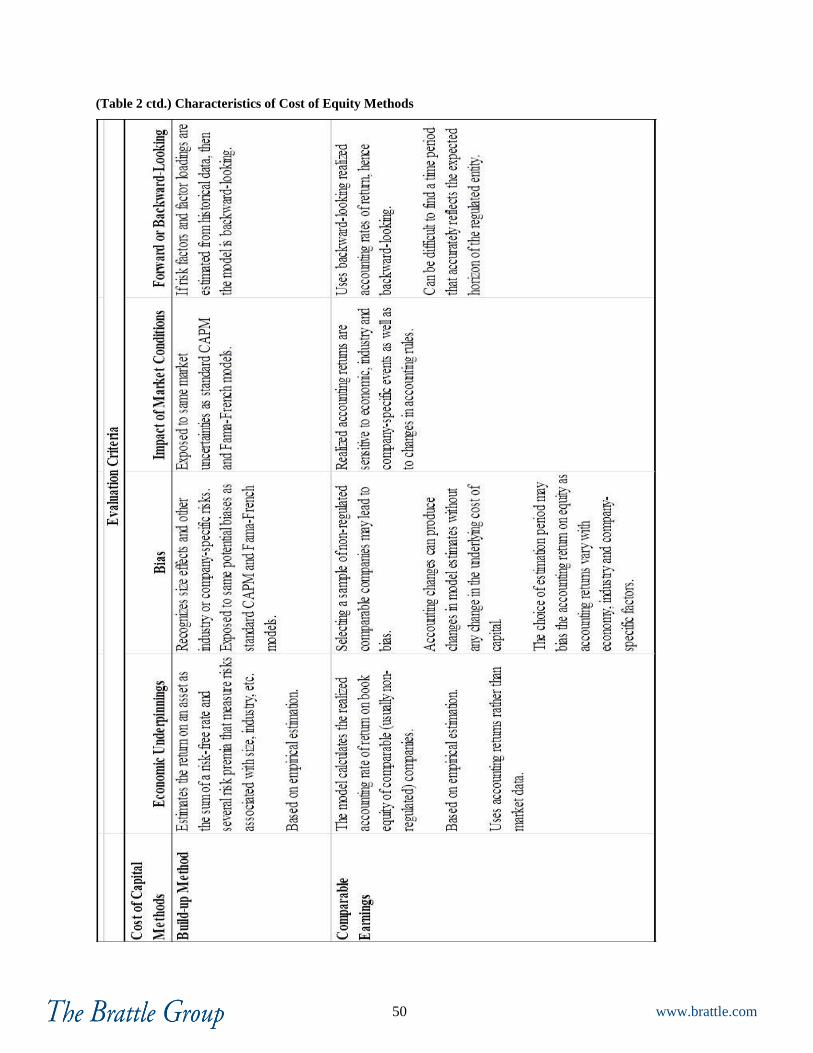
50 www.brattle.com
(Table 2 ctd.) Characteristics of Cost of Equity Methods
51 www.brattle.com
C. HOW TO USE THE MODELS AND OTHER INFORMATION
In this section we discuss how academics, practitioners and regulators think models should be
used and how they have been used. The section also discusses the impact of economic
conditions, industry factors and company-specific issues on the choice of models. The weight
assigned to each model naturally depends on the key characteristics of the cost of equity
estimation models described above. Finally, the section discusses how certain regulators have
decided to use the models in specific economic environments.
1. Views of Academics, Practitioners and Regulators
Academics, practitioners and regulators have all acknowledged that there is no one way to
determine the cost of equity. In the academic literature, several prominent researchers have
commented that the use of more than one method is important. For example, Professor Myers of
the Massachusetts Institute of Technology commented:
Use more than one model when you can. Because estimating the opportunity cost
of capital is difficult, only a fool throws away useful information. That means
you should not use any one model or measure mechanically or exclusively. Beta
is helpful as one tool in a kit, to be used in parallel with DCF models or other
techniques for interpreting capital market data.68
Professors Berk and DeMarzo of Stanford University in their corporate finance textbook
comment on the use of the CAPM, DDM, and other models by practitioners, and state:
In short, there is no clear answer to the question of which technique is used to
measure risk in practice — it very much depends on the organization and the
sector. It is not difficult to see why there is so little consensus in practice about
which technique to use. All the techniques we covered are imprecise. Financial
economics has not yet reached the point where we can provide a theory of
expected returns that gives a precise estimate of the cost of capital. Consider, too,
that all techniques are not equally simple to implement. Because the tradeoff
between simplicity and precision varies across sectors, practitioners apply the
technique that best suit their particular circumstances.69
68
Stewart C. Myers, ―On the Use of Modern Portfolio Theory in Public Utility Rate Cases: Comment,‖ Financial Management, Autumn 1978.
69 Jonathan Berk and Peter DeMarzo, Corporate Finance: The Core, 2009, (Berk & DeMarzo 2009) p. 420.

52 www.brattle.com
Looking to practitioners‘ views, the widely used text, Ibbotson Cost of Capital Yearbook,70
reports results on the cost of equity (and associated weighted average cost of capital) by SIC
code in the U.S. and other countries. In doing so, the yearbook reports the estimated cost of
equity using five estimation methods: Sharpe-Lintner CAPM, CAPM plus/minus a size
premium, Fama-French 3-Factor model, Single-Stage DDM, and 3-Stage DDM. The data source
does not provide specifics on how to use the data but states that:
[r]eaders can select cost of equity from five different models explored in this
book. Given the size of the database being analyzed, there will clearly be
instances where certain cost of equity models will fail to produce useable
numbers. When NMF is displayed in a cost of equity column, it indicates that the
model is producing unreasonable numbers, and greater emphasis should be placed
on other models.71
Similarly, Roger A. Morin, in the context of U.S. regulation, mentions the use of the CAPM,
DDM, risk premium models, and the comparable earnings method, concluding:
No one individual method provides the necessary level of precision for
determining a fair return, but each method provides useful evidence to facilitate
the exercise of an informed judgment. Reliance on any single method or preset
formula is inappropriate when dealing with investor expectations because of
possible measurement difficulties and vagaries in individual companies‘ market
data.72
Looking to regulators, the U.S. Surface Transportation Board (STB) undertook a review of its
cost of equity estimation methodology in 2007-09 in two rounds, focused on the CAPM and
DDM respectively. The STB‘s review resulted in two decisions with detailed instructions on how
to estimate the cost of capital for the railway industry.73
In connection with this review, the STB noted:
70
The most recent version is Morningstar, Ibbotson Cost of Capital 2012 Yearbook (Ibbotson 2012). 71
Ibbotson 2012, p. 6. The text views cost of equity estimates below the risk-free rate and above 50 percent
as being not meaningful. 72
Roger A. Morin, New Regulatory Finance, Public Utilities Reports, Inc., 2006, (Morin 2006) p. 428. 73
Surface Transportation Board, STB Ex Parte No. 664, ―Methodology to be Employed in Determining the
Railroad Industry‘s Cost of Capital,‖ January 17, 2008 (STB 2008) and STB Ex Parte No. 664 (Sub-No.
1), ―Use of a Multi-Stage Discounted Cash Flow Model in Determining the Railroad Industry‘s Cost of
Capital,‖ January 28, 2009 (STB 2009).

53 www.brattle.com
While CAPM is a widely accepted tool for estimating the cost of equity, it has
certain strengths and weaknesses, and it may be complemented by a DCF model.
In theory, both approaches seek to estimate the true cost of equity for a firm, and
if applied correctly should produce the same expected result. The two approaches
simply take different paths towards the same objective. Therefore, by taking an
average of the results from the two approaches, we might be able to obtain a
more reliable, less volatile, and ultimately superior estimate than by relying
on either model standing alone [emphasis added].74
In arriving at this conclusion, the STB took notice of comments from the Federal Reserve that
―multiple models will improve estimation techniques when each model provides new
information,‖75
and also stated that there is ―robust economic literature confirming that, in many
cases, combining forecasts from different models is more accurate than relying on a single
model.‖76
Similarly, the Ontario Energy Board (OEB) reviewed its cost of capital estimation methodology
in 2009 following a year-long process. For context, the OEB does not focus on the cost of
equity, but instead determines the premium over the risk-free rate that rate-regulated utilities are
allowed. Regarding the methods used to determine the so-called Equity Risk Premium (ERP),
the OEB concluded:
the use of multiple tests to directly and indirectly estimate the ERP is a
superior approach to informing its judgment than reliance on a single
methodology.77
Additional examples of regulators who have relied upon multiple cost of equity estimation
models and/or judgment based on a range of evidence are discussed in the section below.
To sum up, as clearly illustrated above, many academics, practitioners and regulators find that it
is preferable to use more than one estimation method to determine the cost of equity. We agree
that it is important to use more than one estimation method and stress that in determining how to
74
STB 2008, p. 2. 75
STB 2009, p. 15. 76
STB 2009, p. 15. 77
Ontario Energy Board, ―EB-2009-0084, Report of the Board on the Cost of Capital for Ontario‘s
Regulated Utilities,‖ Issued December 11, 2009, p. 36 (emphasis in the original).
54 www.brattle.com
weigh the estimation results, it is important to consider the degree to which the information from
the methods overlaps versus providing additional information, the economic and financial
environment that gave rise to the estimates, and the context in which they are being used.
2. Regulatory Practice in using Multiple Models
a) The U.S.
In the U.S., rates for rate-regulated entities are determined by several federal entities as well as
regulators in each of the fifty states and the District of Columbia. Federal regulators tend to have
well-specified methods to determine the cost of equity although they review all the information
put to them. However, state regulators typically do not specify one single method and commonly
have evidence from several estimation methods and parties in front of them before issuing a
decision on the allowed cost of equity. In most cases the state regulator does not specify which
weight was assigned to each method or other evidence. An exception is the determination of the
cost of equity in Mississippi Power‘s Performance Evaluation Plan (PEP), where the Mississippi
Public Service Commission annually updated the cost of equity for the company using a
combination of the CAPM, ECAPM, risk positioning, and the DDM. In this specific
circumstance, the weights assigned to each method are predetermined.78
Some other examples
of U.S. regulators‘ thought processes are provided below.
Surface Transportation Board
The STB used the constant growth model to track the cost of equity for U.S. railroads for a
number of years. However, by 2005 the largest railroads were expanding rapidly and
profitability was increasing. Security analysts were forecasting ―long-run‖ earnings growth for
some railroads at 15% per year. Such growth could not be sustained, so the constant growth
model overstated the true cost of equity by a wide margin. The STB therefore initiated a cost of
capital proceeding to consider how to change the determination of the cost of equity. After
hearing evidence from academics and practitioners, the STB found that:
78
http://www.psc.state.ms.us/.

55 www.brattle.com
if our exploration of this issue has revealed nothing else, it has shown that there is
no single simple or correct way to estimate the cost of equity for the railroad
industry, and countless reasonable options are available.79
As a result of its deliberations the STB eventually settled on a blend of the CAPM and a multi-
stage DDM.80
Georgia
The following example pertaining to Georgia Power, an integrated electric utility, illustrates a
common approach in U.S. state regulation.
Georgia Power is regulated by the Georgia Public Service Commission (Georgia PSC), which
has no pre-set method to determine the cost of equity. In Georgia Power‘s 2010 rate case, an
expert for Georgia Power as well as for the Georgia PSC submitted evidence on the cost of
equity for the company. The company‘s expert estimated the cost of equity using the Sharpe-
Lintner CAPM, a single-stage DDM, and a risk premium approach, and recommended a return
on equity of 11.0 to 11.2%. The PSC staff expert estimated the cost of equity using the Sharpe-
Lintner CAPM, a sustainable growth DDM and also a comparable earnings model for a
recommendation of 9.50 to 10.75%. The Georgia PSC approved a settlement including a cost of
equity of 11.15%, but did not specify how it was arrived at.81
b) Canada
Until the early 1990s, Canadian regulators, much like U.S. state regulators, heard evidence on a
multitude of methods and from various experts before arriving at a decision on the allowed cost
of equity. However, starting in British Columbia in 1994, the British Columbia Utilities
Commission in the first generic cost of capital proceeding in Canada established a benchmark
ROE and a formulaic approach to updating the allowed ROE annually.82
Shortly thereafter,
other Canadian regulators followed suit and similarly established a benchmark ROE and an
79
U.S. Surface Transportation Board, Ex Parte 664 (Sub-No. 1), issued January 28, 2009, p. 15. 80
Ibid. 81
Direct Testimony of J.H. Vande Weide in Docket No. 31958; Direct Testimony of D. Parcell in Docket
No. 31958, and Settlement Agreement in Docket No. 31958. 82
BCUC Decision in the Matter of Return on Common Equity BC Gas Utility Ltd., Pacific Northern Gas
Ltd., West Kootenay Power Ltd., June 10, 1994 (BCUC 1994 Decision), pp. 39-40.

56 www.brattle.com
annual updating formula. These formulae were linked to the change or forecasted change in
government bond yields.
While the formula used to update the allowed ROE annually was mechanical, the methods used
to estimate the benchmark ROE varied across jurisdictions, and in many jurisdictions, the
regulator looked to more than one estimation method.83
As the yield on government bonds declined, so did the allowed cost of equity, and as the
financial crisis of 2008 impacted financial markets, regulators in Canada abandoned or modified
the formula or the relied-upon benchmark. As was the case for the originally developed
benchmark, the regulators heard evidence on multiple methods from several experts and
implicitly or explicitly weighted these methods to arrive at a new or modified cost of equity
methodology.84
Some examples of this regulatory approach in Canada are provided below.
British Columbia
British Columbia Utilities Commission‘s (BCUC) views on how to determine the appropriate
cost of equity capital have evolved over time. In the BCUC 1994 Decision,85
the BCUC ―placed
primary reliance on the various risk premium tests presented‖ whereas the ―comparable earnings
and DCF test results have been used primarily as a check upon reasonableness.‖86
However, in
the BCUC 2006 Decision, the BCUC assigned weight to the DCF model and found the
comparable earnings methodology useful.87
The BCUC 2006 Decision did not state how much
weight it assigned to each model it considered. The BCUC‘s views evolved as the various
83
For example, the BCUC 1994 Decision at p. 17 indicated that while primary reliance should be placed on
risk premium tests, comparable earnings and the DDM should be used as checks. 84
For example, the National Energy Board abandoned the formulaic approach, the Alberta Utilities Board
modified the benchmark, and the Ontario Energy Board modified both the benchmark and the formula.
Both the Alberta Utilities Board and the Ontario Energy Board used several cost of equity estimation
methods to arrive at their revised benchmark. The British Columbia Utilities Commission is in the midst
of a generic cost of capital proceeding that will determine the approach going forward. 85
BCUC Decision in the Matter of Return on Common Equity BC Gas Utility Ltd., Pacific Northern Gas
Ltd., West Kootenay Power Ltd., June 10, 1994 (BCUC 1994 Decision). 86
BCUC 1994 Decision, p. 17. 87
BCUC In the Matter of Terasen Gas Inc. et al. Return on Equity and Capital Structure Decision, December
16, 2009 (BCUC 2009 Decision), pp. 44-45.
57 www.brattle.com
models arrived at more or less plausible results. For example, in its 2009 decision, the BCUC
found:
The Commission Panel agrees that a single variable is unlikely to capture the
many causes of changes in ROE and that in particular the recent flight to quality
has driven down the yield on long-term Canada bonds, while the cost of risk has
been priced upwards.88
Having acknowledged the influence of the current economic environment, the BCUC in 2009
gave the most weight to the DDM, less weight to the Equity Risk Premium method and CAPM,
and a low weight to the comparable earnings model. While the BCUC acknowledged giving
weight to the DDM, ERP, CAPM and comparable earnings method, it did not specify the exact
weights used.89
The BCUC is currently undertaking a review of its cost of capital estimation
methodology.
Ontario Energy Board
The Ontario Energy Board (―OEB‖) regulates electric and gas utilities in Ontario and sets rates
for electric and natural gas distribution and transmission. The OEB also regulates other aspects
of the electric and natural gas sector, but it does not regulate competitive electric or gas supply.
In addition to determining the allowed cost of capital, the OEB also determines a deemed
(allowed) capital structure for the utilities it regulates, and the allowed cost of equity is applied to
the deemed equity portion of the allowed rate base, which is based on historical cost.
The OEB reviewed its approach to determining the cost of capital for Ontario utilities and in
December 2009 issued a report on its estimation procedures going forward.90
Prior to the
review, the OEB relied on a formula-based approach using a version of the risk premium
approach, or Equity Risk Premium (ERP) method to determine the return on common equity.
Although a number of concerns were raised with this approach, the OEB decided to continue
88
BCUC 2009 Decision, p. 73. 89
BCUC 2009 Decision, p. 45. 90
Ontario Energy Board, ―EB-2009-0084, Report of the Board on the Cost of Capital for Ontario‘s
Regulated Utilities,‖ Issued December 11, 2009 (OEB Report 2009).

58 www.brattle.com
relying on a formula-based methodology and the ERP method, but the review led to a resetting
of the risk premium and an adjustment to the formula used to update the ROE.
The OEB‘s current approach to cost-of-capital estimation requires that the Board determine a
baseline ROE and subsequently update the estimate annually using the determined formula. The
baseline ROE was most recently determined in 2009 during the generic proceeding. To arrive at
its initial estimate of the ERP for determining the baseline ROE, the OEB reviewed the
recommendations of the submissions as part of the 2009 proceeding, and determined each
submission‘s Low, Medium, and High ERP.91
In determining the initial ERP, the OEB found
that:
the use of multiple tests to directly and indirectly estimate the ERP is a
superior approach to informing its judgment than reliance on a single
methodology.92
As a result, the OEB considered all submissions, which included estimates based on the CAPM,
DDM, risk premium model, econometric ERP analyses, realized ERP analyses, the difference
between awarded ROEs and realized government bond yields, and various forecasts. The OEB
averaged the experts‘ calculations of the risk premium over the long-term government bond and
used judgment to determine that an appropriate premium over long-term government bonds was
in the low-end of the range determined by the averages of the experts‘ ranges.
c) The U.K.
The U.K. regulator Ofgem has for many years made its cost of equity decisions within a CAPM
framework, and, at least in a formal sense, has published CAPM parameters which correspond to
its cost of equity determinations. However, it is also clear that Ofgem does not treat the CAPM
estimates mechanistically, and, in any case, Ofgem uses a degree of judgment in determining the
equity beta parameter, since there is little direct market evidence that can be relied on. While
some of Ofgem‘s analysis and discussion of utility submissions is framed in terms of the CAPM
parameters, it is clear that Ofgem focuses much more on the final cost of equity figure than on
91
OEB 2009, p. 38. 92
OEB 2009, p. 36 (emphasis in the original).

59 www.brattle.com
the mechanistic derivation of that figure, whether in a CAPM framework or otherwise. For
example, Ofgem has said: ―Overall, our Final Proposals retain the cost of equity assumptions in
our Initial Proposals of 7.0 percent for NGET and 6.8 percent for NGGT. Table 3.5 shows our
Final Proposals for the cost of equity in terms of the CAPM components. We note, however, that
it is the overall allowed return that matters. [emphasis added]‖93
3. Impact of Economic, Industry or Company Factors
It makes sense that multiple cost of equity estimation methods have been developed and remain
in use for a variety of reasons as articulated by Professors Berk and DeMarzo: ―[a]ll the
techniques … are imprecise‖ and ―practitioners apply the technique that best suit their particular
circumstances.‖94
Because economic, industry, and firm-specific factors vary, it is important to
assess the circumstances under which the models discussed in Section III are and should be used.
a) Economic Factors
As a pertinent example, due to the flight to quality following the financial crisis and subsequent
monetary policy initiatives in many countries, the risk-free rate has been suppressed and is
unusually low. Thus, in a standard implementation of the CAPM, the current risk-free rate
results in a low cost of equity estimate. At the same time, investors have in recent years faced
unusually high market volatility as measured by, for example, the S&P / ASX volatility index or
the S&P 500 volatility index.95
Academic literature finds that investors expect a higher risk
premium during more volatile periods. For example, French, Schwert, and Stambaugh (1987)
find a positive relationship between the expected market risk premium and volatility:
We find evidence that the expected market risk premium (the expected return on a
stock portfolio minus the Treasury bill yield) is positively related to the
predictable volatility of stock returns. There is also evidence that unexpected
stock returns are negatively related to the unexpected change in the volatility of
93
RIIO-T1: Final Proposals for National Grid Electricity Transmission and National Grid Gas, Ofgem, 17
December 2012, paragraph 3.45. 94
Berk & DeMarzo 2009, p. 420. 95
The S&P/ASX Volatility Index and the S&P 500 Volatility Index reflect the markets‘ expected volatility
in the benchmark Australian and American equity indices, respectively.

60 www.brattle.com
stock returns. This negative relation provides indirect evidence of a positive
relation between expected risk premiums and volatility.96
And Kim, Morley and Nelson (2004) find:
When the effects of volatility feedback are fully taken into account, the empirical
evidence supports a significant positive relationship between stock market
volatility and the equity premium.97
Other academic papers have found a relationship between general economic conditions and the
MRP. Constantinides (2008) studies a classical utility model where consumers are risk-averse
and also summarizes some of the empirical literature. Empirical evidence shows that consumers
become more risk-averse in times of economic recession or downturn, and equity investments
accentuate this risk.98
Increased risk aversion leads to a higher expected return for investors
before they will invest. Specifically, equities are pro-cyclical and their performance is positively
correlated with the economy‘s performance. Thus, unlike government bonds, equities fail to
hedge against income shocks that are more likely to occur during recessions.99
As a result,
investors require an added risk premium to hold equities during economic downturns.
The very low current risk-free rates make the cost of equity estimates from a standard
implementation of the Sharpe-Lintner CAPM also very low at a time when volatility measures
indicate that the MRP has increased as well. Therefore, these market circumstances call for a
serious consideration of economic factors or other models rather than a mechanical
implementation of the Sharpe-Lintner CAPM.
Conditional models such as the Consumption CAPM attempt to incorporate the relationship
between market volatility and the MRP in determining the cost of equity. As the model
96
K. French, W. Schwert and R. Stambaugh (1987), ―Expected Stock Returns and Volatility,‖ Journal of
Financial Economics, Vol. 19, pp. 3. 97
C-J. Kim, J.C. Morley and C.R. Nelson (2004), ―Is There a Positive Relationship Between Stock Market
Volatility and the Equity Premium?,‖ Journal of Money, Credit and Banking, Vol. 36, p. 357. 98
Constantinides, G.M. (2008), ―Understanding the equity risk premium puzzle,‖ In R. Mehra, ed.,
Handbook of the Equity Risk Premium, Elsevier, Amsterdam. 99
Constantinides, G.M., and D. Duffie (1996), ―Asset Pricing with Heterogeneous Consumers,‖ Journal of
Political Economy, pp. 219-240. See also E.S. Mayfield (2004), ―Estimating the market risk premium,‖
Journal of Financial Economics, vol. 73, pp. 465-496.

61 www.brattle.com
estimates a relationship between the risk premium of a stock and its conditional volatility, the
model allows for a time-varying relationship between risk and return; i.e., the implied cost of
equity varies with the degree to which (i) the underlying stock can serve as a hedge against the
market and (ii) market volatility. As rate-regulated entities commonly move with the market, the
cost of equity estimate usually moves in the same direction as the volatility of the market. Thus,
the consumption-based model addresses the finding that volatility impacts the required risk
premium. As such, it may be particularly useful to implement this model when market volatility
is unusually high or low.100
Given the currently very low risk-free rates and the recent market volatility, the DDM may
additionally provide useful insights into the cost of equity. This is especially true for versions of
the model that take into account (i) all cash that flows to shareholders through not only dividends
but also share buybacks and (ii) changes in the forecasted growth rates in the near term and the
longer term (i.e. multi-stage versions of the DDM).
Table 3 below displays the impact of two key economic factors discussed above, market
volatility and risk-free rates, on the choice of cost of equity estimation model. While there is no
specific formula that can be proposed to select a particular model under given market
circumstances, or a method that can be used to combine the various models mechanistically,
there are certain market scenarios under which it is more appropriate to use one model rather
than another. For example, in times of either extremely high or low market volatility, (or extreme
values of other macroeconomic indicators such as inflation), the consumption-based CAPM
becomes more relevant. The DDM model and especially the multi-stage DDM is also less
sensitive to variations in the risk-free rate than the standard CAPM, but it can be sensitive to
market volatility. This is because in times of economic turmoil, the growth estimates for
companies, including rate-regulated entities, are less likely to be stable going forward. Because
the multi-stage DDM has more realistic characteristics and is less sensitive to analysts‘ short-
term forecasts, the tables in this section use the term DDM to reflect the multi-stage DDM.
100
See Ahern, et al. (2012) for a discussion of its use in a regulatory setting.

62 www.brattle.com
The effect of the risk-free rate and market volatility on model choice is reflected in Table 3
below, which should be viewed as an illustration on the directional choice rather than a
prescription.
Table 3: Relationship Between Key Economic Conditions and Weights to be Given to
Models
b) Industry Factors
As discussed above, empirical research has consistently found that the Security Market Line
determined by the Sharpe-Lintner CAPM (as depicted in Figure 2) is too steep.101
This result is
also consistent with the findings of Fama & French (1992), which estimated a zero slope in the
empirical SML.102
Thus, the ECAPM as well as the Fama-French model attempt to find a model
that is a better fit with empirical data from tests of the Shape-Lintner CAPM, showing that the
latter tends to under estimate the cost of equity for companies with beta estimates below one, and
over estimate the cost of equity for companies with beta estimates above one. A better-fitting
model flattens the Security Market Line as depicted in Figure 3. Because most rate-regulated
entities have beta estimates below one, reliance on the Sharpe-Lintner CAPM tends to bias the
101
See, for example, F. Black, M.C. Jensen, and M. Scholes, ―The Capital Asset Pricing Model: Some
Empirical Tests,‖ Studies in the Theory of Capital Markets, Praeger Publishers, 1972, pp. 79-121 and E.F.
Fama and J.D. MacBeth, ―Risk, Returns and Equilibrium: Empirical Tests,‖ Journal of Political Economy
81 (3), 1972, pp. 607-636. 102
E.F. Fama and K.R. French, ―The Cross-Section of Expected Returns,‖ Journal of Finance 47, 1992, pp.
427-465.

63 www.brattle.com
cost of equity estimates for these companies downwards. Therefore, for entities whose beta
estimates are farther from one, it becomes important to look to the ECAPM to accurately reflect
the cost of equity for the entity.103
In many countries or regions, including Australia, Canada,
Europe and the U.S, estimated betas for rate-regulated entities declined and become statistically
insignificant in the early 2000s as the dot.com bubble burst. In such circumstances, the
downward bias in the cost of equity estimates from the Sharpe-Lintner CAPM becomes more
pronounced and models such as the ECAPM can improve the estimation.
For some industries the future may look like the past, but for others this is not the case. As an
example, the outlook for the U.S shale gas industry today is different than it was in 2008.
Similarly, the outlook for the nuclear industry in Japan changed dramatically after the 2011
tsunami. In such circumstances, forward-looking estimates of the industry‘s cost of capital as
obtained through, for example, versions of the DDM, may be especially useful. As noted above,
the DDM implementation should carefully consider not only the current economic environment
but also industry and firm-specific factors, such as the sustainability of the current growth
forecasts and whether dividends truly reflect all cash distribution to shareholders. For example,
the multi-stage models discussed in Section III rely on several growth rates and therefore enable
the analyst to consider near-term, intermediate, and long-term growth prospects for the
individual company, industry, and economy. Therefore, a multi-stage DDM model, unlike the
Sharpe-Lintner CAPM, can capture both near-term and longer-term changes in an industry. This
becomes especially important when an industry‘s expected risk characteristics differ from its past
characteristics.
Rate-Regulated Entities vs. Other Industries
According to empirical studies, the Sharpe-Lintner CAPM remains the most commonly used
model across the full spectrum of companies.104
However, the utility industry and rate-regulated
entities have some unique characteristics that make it plausible that the methods that serve other
103
See Table A-1 in the Appendix for details. Much of the academic literature estimating alpha dates back to
the 1980s. Academic research has since turned to the Fama-French multifactor model, which attempts to
explicitly capture the empirical pivot of the SML as a function of additional pricing factors. 104
J.R. Graham and C.R. Harvey, ―The Theory and Practice of Corporate Finance: Evidence from the Field,‖
Journal of Financial Economics 60, 2001, pp. 187-243.

64 www.brattle.com
industries well do not serve this industry nearly as well. For example, the utility industry tends
to be relatively stable, so that the DDM (and especially the multi-stage DDM) is much more
likely to provide usable results for this industry than for more volatile industries. As the residual
income valuation model is a variation of the multi-stage DDM, the same comments pertain to
this model.
Prior to the financial crisis, models such as the single-stage DDM, Brattle‘s multi-stage DDM,
the CAPM, and versions of the ECAPM resulted in fairly similar results. Figure 5 below
illustrates this for the gas distribution industry in the U.S. towards the end of 2006. Specifically,
the figure is based on implementing the constant growth DDM, a 3-stage DDM, the Sharpe-
Lintner CAPM, the ECAPM with an alpha of 0.5% and an ECAPM with an alpha of 1.5% for
seven gas distribution companies. Figure 5 then shows the range of the cost of equity estimates
assuming a 50-50 gearing for the target company. The figure also indicates the average cost of
equity obtained from the sample, which is at the split of each bar.
Figure 5
7.0%
8.0%
9.0%
10.0%
11.0%
12.0%
13.0%
14.0%
DDM Multi-Stage
DDM
CAPM ECAPM
(0.5%)
ECAPM
(1.5%)
Co
st o
f E
qu
ity
Source: Calculated by The Brattle Group.
Max
Min
Average

65 www.brattle.com
It is clear from Figure 5 above that there is substantial overlap in the estimates. We attribute this
effect to the fact that the economy was relatively stable in 2006 and so was the gas distribution
industry. At the time, these models largely confirmed the range of the cost of equity estimates.
As discussed above, rate-regulated companies also tend to be low-beta entities, so the empirical
finding that the SML predicted by the Sharpe-Lintner CAPM is too steep is a serious concern for
this industry; i.e., it becomes important to use the ECAPM or other models to ensure that this
empirical observation is accurately reflected in the cost of equity estimates.
Analogously to Table 3, Table 4, Panels A and B below summarize the directional weighing of
the models depending on various industry characteristics. The two industry factors considered in
Table 4, Panel A below are the stability of growth rate forecasts and the average market beta of
the industry. For example, as mentioned above, rate-regulated entities tend to have relatively
more stable growth forecasts over time and low betas (i.e., beta estimates below one). Therefore,
for this industry, the use of the ECAPM or variations of the multi-stage DDM might become
valuable in determining the cost of equity capital. The effect of the stability of growth forecasts
and the beta value on model choice is reflected in Table 4, Panel A below, which should be
viewed as an illustration on the directional choice rather than a prescription.
Table 4: Relationship Between Key Industry Factors and Weights to be given to Models–
Panel A
Another characteristic of the industry that should be considered is whether companies in the
industry are exposed to financial distress and/or significant merger and acquisition activity, and
Stability of Industry Growth Forecasts Over Time
Mark
et
Beta
of
Ind
ustr
y
High Average Low
High ECAPM / DDM ECAPM / Other
Average CAPM / DDM CAPM / Other
Low ECAPM / DDM ECAPM / Other

66 www.brattle.com
the prevalence of share buybacks. As discussed above, market-based estimation models are
relatively more affected when a given company faces financial distress, or unique circumstances
that may lead to its stock price decoupling from fundamentals. Therefore, if many companies in
an industry are subject to such effects, the whole industry may be affected. Further, companies
that engage in a substantial amount of share buybacks will end up distributing cash to
shareholders in a form other than dividends, which makes a DDM based on a per share dividend
ratio less appropriate. Panel B below illustrates these effects.
Table 4: Relationship Between Key Industry Factors and Weights to be given to Models–
Panel B
c) Company Factors
In many instances company-specific issues are better dealt with via sample selection or through
risk positioning than through the determination of how to estimate the cost of equity. A
company that is a potential member of the benchmark sample is often dropped if it faces unique
circumstances that may bias the cost of capital estimation process. This is the case if, for
example, a company is undergoing significant merger or acquisition activity, which inherently
affects the information available in the market and therefore drives the stock price (and thus the
results from all market-based models, including the CAPM, ECAPM, Fama-French and DDM).
Industry Exposure to Financial Distress and/or M&A
Pre
va
len
ce o
f S
ha
re B
uyb
ack
s High Low
High
Other Models: Risk
Premium, comparable
earnings, maybe use
other industries
CAPM, ECAPM, DDM that
includes all cash that accrues
to shareholders
Low CAPM, ECAPM, DDM
67 www.brattle.com
After a range of cost of equity estimates has been obtained, it is necessary to consider where,
from within this range, the final determination on the cost of equity will be. Provided that the
range has been developed in an appropriate way that takes account of the market and industry
factors described in this section, the final step is to consider the relative risk of the target
company compared to the sample of companies from which the cost of equity range has been
developed. The cost of equity is adjusted upward or downward depending on the target entity‘s
risk characteristics relative to those of the sample. This issue is the topic of the next section.
D. RISK POSITIONING OF THE TARGET ENTITY
The discussion in the preceding sections covered various models that produce cost of equity
estimates. Typically the cost of equity will be estimated for a sample of firms, or all firms in a
particular sector, because it usually is not possible to estimate the cost of equity for a single firm
with a useful degree of accuracy. To determine a single value for the cost of equity for a specific
firm from a range of values for a set of comparator firms, it makes sense to consider the riskiness
of the specific firm relative to the riskiness of the sample, since the cost of equity itself is
compensating investors for risk.
In the regulatory context, in some cases this process is implicit in the regulator‘s decision, while
in others it is an explicit step in the cost of equity determination process. This step can
conveniently be termed ―risk positioning‖, because the regulator considers the risk characteristics
of the specific utility relative to the benchmark.
1. Why risk positioning is necessary
While the precise details and wording of the regulator‘s objective in setting the cost of equity
vary from one jurisdiction to another, the underlying idea is that investors will expect a return
equivalent to the return that they would expect from other investments of like risk. Utilities
generally have low risk relative to the market as a whole, but within the utilities sector, different
firms are likely to have somewhat different risk characteristics. ―Risk positioning‖ acknowledges
the possibility that different utilities can have somewhat different risks. In this context, ―risk‖ is
defined as the characteristic of an investment which determines expected returns which would
usually include ―systematic‖ exposure to the wider economy, but not ―idiosyncratic‖ risks
associated with specific projects that can be diversified away in an investment portfolio. While

68 www.brattle.com
the cost of equity solely captures investors‘ compensation for bearing systematic risk, the cost of
debt reflects total risk, including idiosyncratic risks. Therefore, there are instances of regulatory
mechanisms, such as decoupling, which reduce the variability of total revenues and therefore
also total risk, (affecting the cost of debt), but which may not impact the cost of equity for a
given utility.
One way in which a utility is exposed to systematic risk is through variations in demand. End-
user demand tends to be at least somewhat correlated with wider economic activity, and is thus a
source of exposure to systematic risk. One utility might have more exposure than other, for
example if it has a greater proportion of price-sensitive industrial load.
In some jurisdictions, leverage is considered a source of ―financial risk‖, which affects the risk
positioning analysis. This could be so, for example, where the rate of return is generally
determined on the basis of actual capital structure. A utility with more debt than the benchmark
will require a higher return on equity than the benchmark, even if it otherwise has similar
business risk exposure as the benchmark (just as two utilities with the same asset beta would
have different equity betas if one has higher gearing than the other). Where this approach is
taken, the term ―business risk‖ is used to refer to the other sources of relevant risk differences
that are taken into account in the risk positioning analysis.
Once a benchmark rate of return has been defined (whether a point estimate or a range), the risk
positioning approach requires an analysis of the particular utility‘s risk relative to that
benchmark. To the extent that the utility is found to have more (or less) risk than the benchmark,
the rate of return would be set higher (or lower) than the benchmark rate of return.
2. What risk characteristics are relevant?
The characteristics relevant to risk positioning are those which expose the utility to systematic
risk and which therefore have an impact on the rate of return required by investors. Some
important sources of uncertainty in revenues and returns to investors may not have an impact on
the required return to the extent that investors are able to diversify away exposure to those risks.
For example, the weather may be an important source of variability in revenues and returns, but
may not be an important source of risk to investors because it is diversifiable.

69 www.brattle.com
A good way to think about risk positioning is to consider the extent to which different utilities
are protected from risks. A distribution utility can in principle be protected from risks to the
extent that it is able to pass on risk to its customers (which depends on the detail of the
regulatory framework being applied). Demand risk (which is at least partly non-diversifiable),
for example, can be borne by the utility if the regulatory regime sets prices and does not ―true
up‖ revenues to account for the difference between forecast and actual demand. Alternatively,
demand risk can be passed on to customers through a true-up or balancing account process,
which would allow the utility to recover in one year any ―missing‖ revenue from the prior year
caused by demand forecasting errors. Protection from demand risk in this way depends on both a
regulatory framework that allows for such true-ups and on the existence of franchise customers
that will bear the risks passed on to them. Therefore, other things equal, a utility with true-ups for
demand risk would be considered less risky than one without.
Distribution utilities typically have franchise customers that rely on the utility and have no
alternative supply of energy. However, this is typically not the case for gas pipelines: in many
jurisdictions, gas pipelines do not have ―franchise‖ customers: customers may be free to switch
to competing pipelines. Even if there is no prospect of competition from other pipelines, it may
still be difficult for pipelines to pass on demand risk to their customers, since large end-users
may be price sensitive (i.e., if the pipeline increases price in response to a fall in demand, the
price increase itself could further cut demand).
Pipeline regulators in both the US and Canada apply a risk-positioning approach in determining
the cost of equity.
3. FERC Approach
The Federal Energy Regulatory Commission (FERC) has a standard approach to determining the
cost of equity for gas pipelines, set out in a ―policy statement‖,105
which, together with precedent
from prior decisions, guides all decisions on the cost of equity for gas pipelines. The FERC‘s
approach is to use a form of the dividend growth model (typically termed the ―DCF‖ model in
105
Composition of Proxy Groups for Determining Gas and Oil Pipeline Return on Equity, FERC (April 2008).

70 www.brattle.com
the US) to estimate the cost of equity for a benchmark group of publicly-traded pipeline
companies. The results of the model are a cost of equity estimate for each of the companies in
the benchmark (or ―proxy‖) group.
FERC starts by assuming that the median company in the proxy group is the appropriate cost of
equity, unless either the pipeline or an intervener in the case demonstrates that the instant
pipeline has risk factors which mean that the cost of equity should be set above or below the
median:
after defining the zone of reasonableness through development of the appropriate proxy
group for the pipeline, the Commission assigns the pipeline a rate within that range or
zone, to reflect specific risks of that pipeline as compared to the proxy group companies.
[f/n omitted] The Commission has historically presumed that existing pipelines fall within
a broad range of average risk. A pipeline or other litigating party has to show highly
unusual circumstances that indicate anomalously high or low risk as compared to other
pipelines to overcome the presumption.106
And
unless a party makes a very persuasive case in support of the need for an adjustment and
the level of the adjustment proposed, the Commission will set the pipeline’s [ROE] at the
median of the range of reasonable returns.107
In line with this approach, most FERC decisions result in the pipeline receiving a cost of equity
equal to the median of the proxy group. A recent decision for El Paso Natural Gas (EPNG),108
however, illustrates how FERC assesses relative risk and may, on occasion, move away from the
median. In this case, the FERC ALJ109
characterized EPNG‘s business risk on two related
dimensions: competitive risk and regulatory risk. US natural gas pipelines typically secure long-
term contractual commitments from shippers to use the pipeline capacity (with relatively high
fixed charges, equivalent to a take-or-pay commitment). EPNG had long-term contracts for a
smaller proportion of its capacity than did the pipelines in the proxy group, and its contracts were
typically shorter. Furthermore, EPNG‘s throughput had been declining. This is symptomatic of
higher business risk, because in the absence of contractual commitments and in the absence of
106
Ibid., p. 4. 107
El Paso Natural Gas Company, Initial Decision, docket no. RP10-1398 (June 18, 2012), paragraph 40,
quoting prior FERC decisions. 108
El Paso Natural Gas Company, Initial Decision, docket no. RP10-1398 (June 18, 2012). 109
A FERC rate case typically results in an ―initial decision‖ issued by an Administrative Law Judge (ALJ).
The ALJ‘s decision is subsequently reviewed by the FERC commissioners, and may be affirmed or varied.

71 www.brattle.com
franchise customers, the pipeline is no longer able to pass on risks to its customers. In the limit,
the pipeline may be unable to charge rates high enough to recover its authorized revenue
requirement (as increasing rates drives throughput lower still).
The ALJ found that EPNG was exposed to competition in its major downstream markets from
new pipeline projects, and that this competition was to an extent the result of regulatory policies
that favor new pipeline projects to foster competition (possibly harming existing pipelines).
Based on this analysis (and also a finding that EPNG had above-average financial risk, as
evidenced by a credit rating of BBB-, lower than all but one of the proxy group companies), the
ALJ determined that EPNG‘s cost of equity should be set ―well above the median ROE [of the
proxy group]‖.110
4. NEB approach
In Canada, the approach taken by energy regulators (both provincial and national) historically
was to set the cost of equity on a formula basis and to us the same cost of equity for all pipelines.
Risk positioning was then used to vary the authorized proportion of equity in the capital
structure, thereby increasing the overall return on capital for those utilities judged to be riskier.
However, in the most recent decision by Canada‘s National Energy Board (NEB), the NEB
moved to an approach which focuses on the overall after-tax return directly, rather than
separately determining the cost of equity, the cost of debt, and the proportion of each in the
capital structure.111
The NEB takes a systematic approach to assessing business risk under the
headings ―supply risk‖, ―market [downstream] risk‖, ―regulatory risk‖, ―competitive risk‖ and
―operating risk‖, although the NEB said ―The various forms of risk are in some cases
inextricably linked, and the boundaries between them are subjective‖.112
In the RH-1-2008
case,113
the NEB was concerned with whether the business risk of the pipeline had increased
110
Ibid., p. 45. The ALJ did not specify an ROE. The final decision on ROE rests with the FERC
commissioners. 111
See RH-1-2008, discussed further below. 112
Reasons for Decision, Trans Quebec and Maritimes Pipelines Inc., RH-1-2008, NEB (March 2009), p. 30. 113
Concerning the Trans Quebec and Maritimes Pipelines, which predominantly move supplies sourced from the Western Canadian Sedimentary Basin (WCSB) via the TransCanada Mainline, into Quebec and on into
New Hampshire.

72 www.brattle.com
since the last time that a decision on the cost of capital for the pipeline had been taken. The NEB
identified a number of factors as contributing to an increased overall business risk.
Supply risk: the pipeline was mainly supplied from a region with declining conventional
production and rising costs. While it was possible that new sources of unconventional
supply (shale gas) would be developed, the result was increased uncertainty over the
availability of competitively-priced supplies, and hence concerns over the possibility for
reduced throughput.
Market and competitive risk: because a large and increased proportion of the pipeline‘s
throughput went to large industrial and electric power generation load, which is more
variable than domestic and commercial load. In addition, competition with cheap hydro-
power in the Quebec also contributed to increased market risk. Market risk was also
increased as a result of the potential for competition with LNG imports in the US market.
Overall, the NEB concluded that business risk had increased as a result of these factors relative
to the previous cost of capital decision for the pipeline. Whereas the FERC in the US uses a risk
positioning approach to determine the cost of equity relative to a benchmark, the NEB estimated
the after-tax weighted average cost of capital directly, principally on the basis of market-based
estimates of the cost of capital of various comparator companies. The business risk analysis
described above was part of the NEB‘s determination of where the pipeline‘s cost of capital
should be relative to the sample data.114
5. Implementation
In the FERC and NEB examples given above, risk positioning of the target utility within the
range of comparator or proxy companies is not analytically precise: the regulator considers
evidence (which could be quantitative, such as the proportion of price-sensitive industrial load,
or more qualitative) as to exposure to various relevant risk factors. Weighing the risk factors, and
determining how the analysis of risk should be reflected in the final cost of equity determination
is necessarily imprecise, and relies on judgment. For example, a regulator might determine that a
114
The NEB‘s analysis is summarized on p.79 of the decision.

73 www.brattle.com
particular utility, having an unusually high proportion of industrial load, was of above average
risk, and that as a result the cost of equity should be 50 basis points above the mid-point of a
range determined for a sample of utilities. The direction of the adjustment (upwards) is clear, but
the magnitude is more a matter of judgment than something that can be derived quantitatively.

74 www.brattle.com
APPENDIX: ADDITIONAL TABLES AND FIGURES
Table A-1: Empirical Evidence On The Alpha Factor in ECAPM
AUTHOR RANGE OF ALPHA PERIOD RELIED UPON
Black (1993)1
1% for betas 0 to
0.80 1931-1991
Black, Jensen and Scholes (1972)2 4.31% 1931-1965
Fama and MacBeth (1972) 5.76% 1935-1968
Fama and French (1992)3 7.32% 1941-1990
Fama and French (2004)4 N/A
Litzenberger and Ramaswamy
(1979)5
5.32% 1936-1977
Litzenberger, Ramaswamy and
Sosin (1980) 1.63% to 3.91% 1926-1978
Pettengill, Sundaram and Mathur
(1995)6
4.6% 1936-1990
* The figures reported in this table are for the longest estimation period available and, when applicable,
use the authors‘ recommended estimation technique. Many of the articles cited also estimate alpha for
sub-periods and those alphas may vary. 1
Black estimates alpha in a one-step procedure rather than in an un-biased two-step procedure. 2
Estimate a negative alpha for the sub period 1931-39 which contain the depression years 1931-33 and
1937-39. 3
Calculated using Ibbotson‘s data for the 30-day treasury yield. 4
The article does not provide a specific estimate of alpha; however, it supports the general finding that
the CAPM underestimates returns for low-beta stocks and overestimates returns for high-beta stocks. 5
Relies on Litzenberger and Ramaswamy‘s before-tax estimation results. Comparable after-tax alpha
estimate is 4.4%. 6
Pettengill, Sundaram and Mathur rely on total returns for the period 1936 through 1990 and use 90-day
treasuries. The 4.6% figure is calculated using auction averages 90-day treasuries back to 1941 as no
other series were found this far back.

75 www.brattle.com
Sources:
Black, Fischer. 1993. Beta and Return. The Journal of Portfolio Management 20 (Fall): 8-18.
Black, F., Michael C. Jensen, and Myron Scholes. 1972. The Capital Asset Pricing Model: Some
Empirical Tests, from Studies in the theory of Capital Markets. In Studies in the Theory of Capital
Markets, edited by Michael C. Jensen, 79-121. New York: Praeger.
Fama, Eugene F. and James D. MacBeth. 1972. Risk, Returns and Equilibrium: Empirical Tests. Journal
of Political Economy 81 (3): 607-636.
Fama, Eugene F. and Kenneth R. French. 1992. The Cross-Section of Expected Stock Returns. Journal of
Finance 47 (June): 427-465.
Fama, Eugene F. and Kenneth R. French. 2004. The Capital Asset Pricing Model: Theory and Evidence.
Journal of Economic Perspectives 18 (3): 25-46.
Litzenberger, Robert H. and Krishna Ramaswamy. 1979. The Effect of Personal Taxes and Dividends on
Capital Asset Prices, Theory and Empirical Evidence. Journal of Financial Economics XX (June): 163-
195.
Litzenberger, Robert H. and Krishna Ramaswamy and Howard Sosin. 1980. On the CAPM Approach to
Estimation of a Public Utility's Cost of Equity Capital. The Journal of Finance 35 (2): 369-387.
Pettengill, Glenn N., Sridhar Sundaram and Ike Mathur. 1995. The Conditional Relation between Beta
and Returns. Journal of Financial and Quantitative Analysis 30 (1): 101-116.

1
SCHEDULE 3: The differences between Gas and Electricity
Businesses and the impact on the cost of capital to them
Differing risks for gas and electricity investment
There are many differences across gas and electricity markets and assets. APIA considers
that three key differences:
usage in the economy;
the contract carriage model of gas; and
the setting of wholesale price
create substantially different risk profiles for gas and electricity supply infrastructure and
mean investments in each are not considered interchangeable by financial and capital
markets.
Gas and electricity supply assets have different risks and compete for capital on differing basis.
It is evident to APIA that there are materially different risks facing investors in energy supply
infrastructure, between electricity and gas assets, between gas transmission and distribution
assets and between gas transmission assets.
Gas and electricity are used differently in the economy
Electricity is a fuel of necessity. Virtually all Australian households and businesses are
connected to the electricity supply grid and in all jurisdictions connection is a legislated right.
The electricity industry serves all sectors of the economy, including the heavy industrial sectors,
manufacturing and processing, retail, schools, hospitals and governments, right down to the
individual household level.
In contrast, gas is a discretionary fuel in many markets.
The penetration of gas into the retail marketplace is quite low in Australia, with Victoria
enjoying the greatest depth of penetration at the domestic and small commercial level at
around 70%. Overall, gas penetration across Australia at the domestic and small commercial
level is 41% that of electricity.45
Residential and commercial demand accounted for over 58% of total electricity demand in
2009/10 but only 17% of total gas demand in the same year.
The mining and manufacturing industries are large users of gas, accounting for almost 50%
of total gas demand in 2009/10.
35% of total gas use in Australia is for electricity generation, and gas faces competitive
pressures in the generation market that have no impact on electricity supply infrastructure.

2
Energy supply infrastructure has different exposure to revenue risk
The exposure to different sectors varies across energy supply infrastructure. With its
universal use and heavy exposure to the residential and commercial sectors, the revenue
risk of the electricity supply industry is spread across the fortunes of the economy as a
whole. From an economic regulation point of view, various electricity supply infrastructure
assets have reasonably equivalent exposure to these risks.
Gas supply infrastructure does not share this characteristic. The utilisation of gas supply
infrastructure, and therefore revenue, is more dependent on an individual asset’s exposure
to large industrial customers.
At the gas distribution level, an asset’s utilisation depends on its level of penetration and the
number of large industrial and commercial customers connected to the network, and this
varies across states. Penetration ranges from 70% in Victoria, around 40% in NSW and WA,
to below 10% in QLD. There are over 800 large industrial and commercial customers
connected in Victoria, around 450 connected in NSW and less than 200 connected in
Queensland, South Australia and Western Australia.48
This impact is more pronounced at the gas transmission level, and its fortunes can depend
on a relatively small number of very large users unique to the asset. An indication of the
customers of regulated gas transmission assets is provided below.
Revenue models of energy supply infrastructure
There are fundamental differences in the revenue models of gas and electricity supply
infrastructure, and these are recognised in the provisions of the NER and NGR in the making
of price determinations for electricity supply infrastructure and access arrangements for gas
supply infrastructure.
Access arrangements and bilateral contracts
48
Electricity Gas Australia 2011, Energy Supply Association of Australia

3
The gas industry, globally, is driven by bilaterally agreed contracts. This is a feature of the
global industry that is also apparent in Australia.
Gas transmission and distribution infrastructure generates revenue through bilateral
contracts, negotiated by parties to specifically tailor transportation services to suit the needs
of the shippers.
This bilateral contracting feature has been in place much longer than the Australian access
regime. For example, the Roma Brisbane pipeline was constructed in 1969, long before
Australia’s Third Party Access Regime was developed. The RBP has always been an open
access pipeline, with that access governed by the bilateral contracts in place.
Price determinations
The approval of access arrangements by the AER provides a reference service and tariff for
shippers to contract capacity on gas supply infrastructure. In some cases, shippers will
require the reference service. Often, a shipper will require a specifically tailored service, and
the reference service and tariff will provide a starting point for the negotiation of bilateral
contracts.
This contrasts with the price determinations for electricity supply infrastructure. In this case,
the AER approves an amount of revenue to be recovered from electricity users, which is
then drawn from a pool based on usage of an asset. Users of electricity supply infrastructure
have no direct relationship with owners.
Investment
The bilateral contracting process recognises a sharing of risk between project proponent and
pipeline owner, where both invest significant capital in plant and equipment and pipeline
assets respectively. Each party relies on the other to realise its investment in capital assets.
As gas transmission infrastructure is long lived, investors usually require that a pipeline’s
capacity is contracted appropriately, such that the investment will be recovered in the
required timeframe, prior to committing to invest. In this way, the users of gas transmission
infrastructure drive the delivery of gas transmission capacity.
A gas supply pipeline’s revenue is determined through its bilateral contracts, and it must
invest and operate with the revenue bounds set by its contractual arrangements. This fits in
with the ‘NPV‐positive’ requirement in the NGR, as shown in the following excerpt from Rule
79:
79 New capital expenditure criteria
…
(2) Capital expenditure is justifiable if:
….

4
(b) the present value of the expected incremental revenue to be generated as a result of the
expenditure exceeds the present value of the capital expenditure; or
…
This NPV‐positive criteria invariably drives transmission pipeline investment to be
underwritten by bilateral contracts supporting the revenue side of the equation.
Importantly, bilateral contracting is not a feature of the electricity industry. This is clearly
reflected in the capital expenditure requirements in the NEL, where the capital expenditure
objectives are stated in terms of meeting demand, comply with obligations, maintain
quality, reliability, safety and security – there is no revenue discipline in the electricity capex
objectives of the NEL sections 6.5.7 and 6A.6.7:
6.5.7 Forecast capital expenditure
(a) A building block proposal must include the total forecast capital expenditure for the
relevant regulatory control period which the Distribution Network Service Provider considers
is required in order to achieve each of the following (the capital expenditure objectives):
(1) meet or manage the expected demand for standard control services over that period;
(2) comply with all applicable regulatory obligations or requirements associated with the
provision of standard control services;
(3) maintain the quality, reliability and security of supply of standard control services;
(4) maintain the reliability, safety and security of the distribution system through the supply
of standard control services.
and
6A.6.7 Forecast capital expenditure
(a) A Revenue Proposal must include the total forecast capital expenditure for the relevant
regulatory control period which the Transmission Network Service Provider considers is
required in order to achieve each of the following (‘the capital expenditure objectives’):
(1) meet the expected demand for prescribed transmission services over that period;
(2) comply with all applicable regulatory obligations or requirements associated with the
provision of prescribed transmission services;
(3) maintain the quality, reliability and security of supply of prescribed transmission services;
and
(4) maintain the reliability, safety and security of the transmission system through the supply
of prescribed transmission services.
Differing contractual arrangement across assets also expose assets to different risks. For
example, the introduction of the Clean Energy Act 2011 in November this year introduces a
carbon price to the Australian economy from 1 July 2012. The bilateral contracts of the gas
transmission industry are not all equipped with the necessary provisions to appropriately
allocate this cost, depending largely on the vintage of the contracts. This is not an issue for
electricity supply infrastructure or gas distribution infrastructure, which will have the costs
managed through regulated revenue.
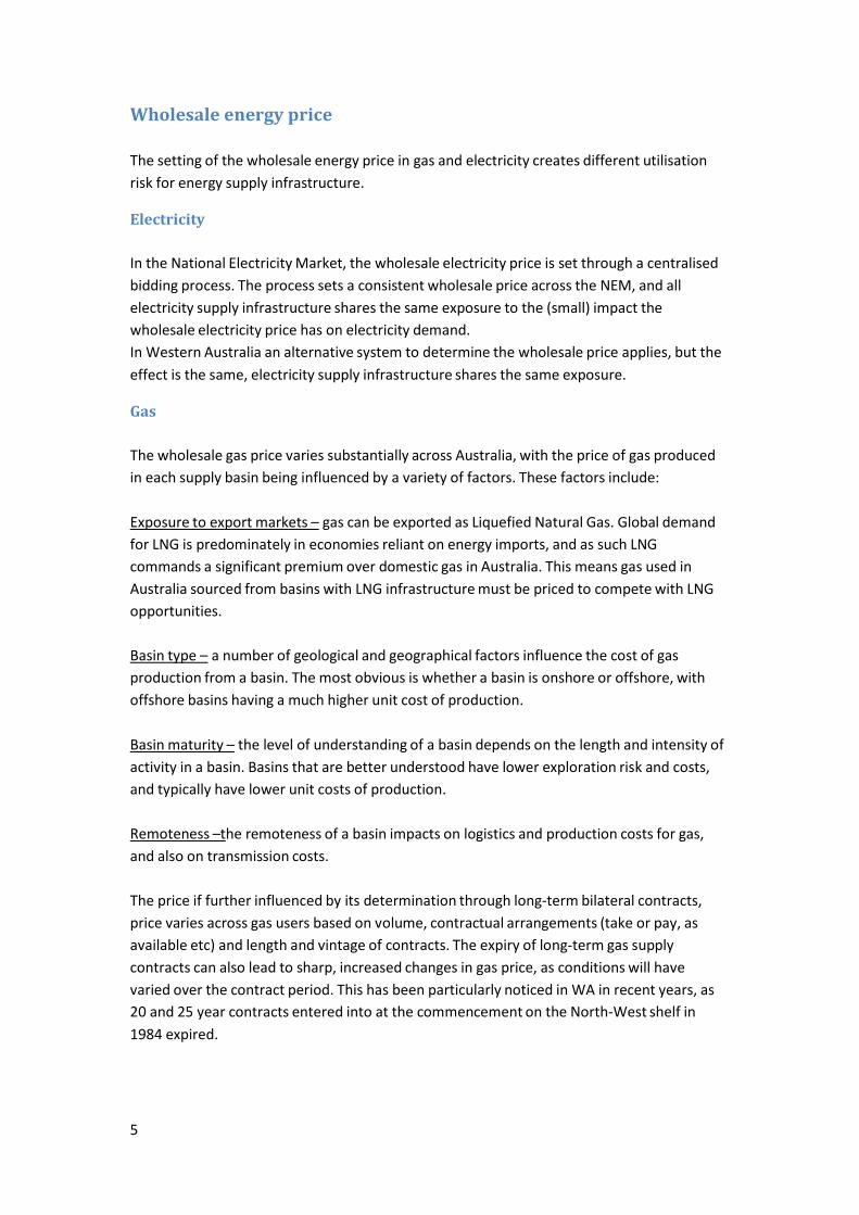
5
Wholesale energy price
The setting of the wholesale energy price in gas and electricity creates different utilisation
risk for energy supply infrastructure.
Electricity
In the National Electricity Market, the wholesale electricity price is set through a centralised
bidding process. The process sets a consistent wholesale price across the NEM, and all
electricity supply infrastructure shares the same exposure to the (small) impact the
wholesale electricity price has on electricity demand.
In Western Australia an alternative system to determine the wholesale price applies, but the
effect is the same, electricity supply infrastructure shares the same exposure.
Gas
The wholesale gas price varies substantially across Australia, with the price of gas produced
in each supply basin being influenced by a variety of factors. These factors include:
Exposure to export markets – gas can be exported as Liquefied Natural Gas. Global demand
for LNG is predominately in economies reliant on energy imports, and as such LNG
commands a significant premium over domestic gas in Australia. This means gas used in
Australia sourced from basins with LNG infrastructure must be priced to compete with LNG
opportunities.
Basin type – a number of geological and geographical factors influence the cost of gas
production from a basin. The most obvious is whether a basin is onshore or offshore, with
offshore basins having a much higher unit cost of production.
Basin maturity – the level of understanding of a basin depends on the length and intensity of
activity in a basin. Basins that are better understood have lower exploration risk and costs,
and typically have lower unit costs of production.
Remoteness –the remoteness of a basin impacts on logistics and production costs for gas,
and also on transmission costs.
The price if further influenced by its determination through long‐term bilateral contracts,
price varies across gas users based on volume, contractual arrangements (take or pay, as
available etc) and length and vintage of contracts. The expiry of long‐term gas supply
contracts can also lead to sharp, increased changes in gas price, as conditions will have
varied over the contract period. This has been particularly noticed in WA in recent years, as
20 and 25 year contracts entered into at the commencement on the North‐West shelf in
1984 expired.
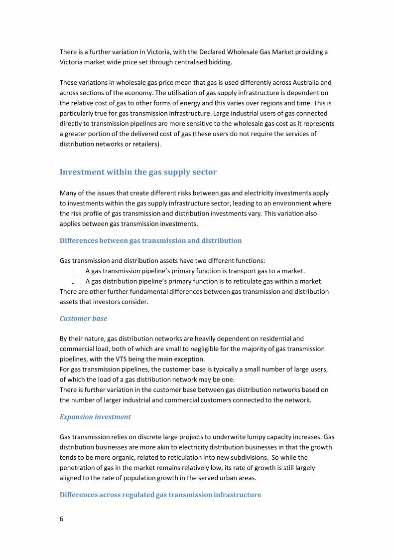
6
There is a further variation in Victoria, with the Declared Wholesale Gas Market providing a
Victoria market wide price set through centralised bidding.
These variations in wholesale gas price mean that gas is used differently across Australia and
across sections of the economy. The utilisation of gas supply infrastructure is dependent on
the relative cost of gas to other forms of energy and this varies over regions and time. This is
particularly true for gas transmission infrastructure. Large industrial users of gas connected
directly to transmission pipelines are more sensitive to the wholesale gas cost as it represents
a greater portion of the delivered cost of gas (these users do not require the services of
distribution networks or retailers).
Investment within the gas supply sector
Many of the issues that create different risks between gas and electricity investments apply
to investments within the gas supply infrastructure sector, leading to an environment where
the risk profile of gas transmission and distribution investments vary. This variation also
applies between gas transmission investments.
Differences between gas transmission and distribution
Gas transmission and distribution assets have two different functions:
A gas transmission pipeline’s primary function is transport gas to a market.
A gas distribution pipeline’s primary function is to reticulate gas within a market.
There are other further fundamental differences between gas transmission and distribution
assets that investors consider.
Customer base
By their nature, gas distribution networks are heavily dependent on residential and
commercial load, both of which are small to negligible for the majority of gas transmission
pipelines, with the VTS being the main exception.
For gas transmission pipelines, the customer base is typically a small number of large users,
of which the load of a gas distribution network may be one.
There is further variation in the customer base between gas distribution networks based on
the number of larger industrial and commercial customers connected to the network.
Expansion investment
Gas transmission relies on discrete large projects to underwrite lumpy capacity increases. Gas
distribution businesses are more akin to electricity distribution businesses in that the growth
tends to be more organic, related to reticulation into new subdivisions. So while the
penetration of gas in the market remains relatively low, its rate of growth is still largely
aligned to the rate of population growth in the served urban areas.
Differences across regulated gas transmission infrastructure

7
The unique aspects of gas supply assets extend beyond the differences between
transmission and distribution. Unlike the electricity transmission and distribution or gas
distribution sectors, gas transmission assets are largely unregulated, as they face
competition from each other and other energy alternatives.
Each transmission pipeline has its own start and finish point, transporting differently priced
gas from different sources to different markets.
Each transmission pipeline has its own customer base, with the majority of capacity typically
reliant of a small number of large industrial users. These differing customer bases create
unique demand and utilisation profiles for each pipeline. They also impact the ‘peakiness’ of a
pipeline’s load, which has a direct impact on pricing as a pipeline must be built to meet the
requirements of peak demand, but must generate revenue from utilisation.
Gas transmission is only one component of the delivered cost of gas.
Particularly in times of rising energy commodity process, the cost of gas transportation is a
minor component of the delivered cost of gas. For high level comparison purposes, it is
reasonable to examine the case of the Roma to Brisbane pipeline: the gas transportation
tariff is in the order of 50 cents per GJ, a fraction of the commodity price of gas in the order
of $8‐$10 per GJ.
Gas transmission is a low cost but high importance link in the supply chain.
Pipeline businesses, like many other infrastructure businesses, are very capital intensive by
their nature.
Generally speaking, the regulated return on capital can account for the majority (up to 60%)
of the total revenue requirement of the regulated business. This is particularly the case of
gas transmission pipelines, whose operating costs tend to be a lower proportion of costs
relative to distribution pipelines.
An error in the AER’s assessment of the cost of capital can therefore have a significant effect
on the revenues of the regulated pipeline businesses.
Concentrated costs vs distributed benefits
As discussed above, the cost of gas transmission is a very small component of the delivered
cost of gas.
A reduction in gas pipeline revenues and tariffs will therefore result in very small savings to
individual customers – potentially too small to be noticed in light of other input costs.
Importantly, this small saving is likely to be too small to influence investment decisions of
individual end users.
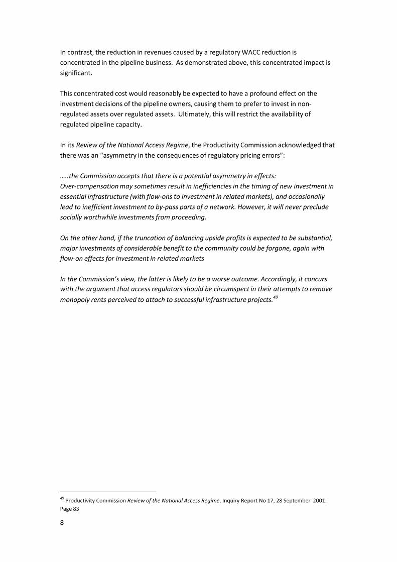
8
In contrast, the reduction in revenues caused by a regulatory WACC reduction is
concentrated in the pipeline business. As demonstrated above, this concentrated impact is
significant.
This concentrated cost would reasonably be expected to have a profound effect on the
investment decisions of the pipeline owners, causing them to prefer to invest in non‐
regulated assets over regulated assets. Ultimately, this will restrict the availability of
regulated pipeline capacity.
In its Review of the National Access Regime, the Productivity Commission acknowledged that
there was an “asymmetry in the consequences of regulatory pricing errors”:
…..the Commission accepts that there is a potential asymmetry in effects:
Over‐compensation may sometimes result in inefficiencies in the timing of new investment in
essential infrastructure (with flow‐ons to investment in related markets), and occasionally
lead to inefficient investment to by‐pass parts of a network. However, it will never preclude
socially worthwhile investments from proceeding.
On the other hand, if the truncation of balancing upside profits is expected to be substantial,
major investments of considerable benefit to the community could be forgone, again with
flow‐on effects for investment in related markets
In the Commission’s view, the latter is likely to be a worse outcome. Accordingly, it concurs
with the argument that access regulators should be circumspect in their attempts to remove
monopoly rents perceived to attach to successful infrastructure projects.49
49 Productivity Commission Review of the National Access Regime, Inquiry Report No 17, 28 September 2001.
Page 83

9
Map of Australia’s gas transmission infrastructure and gas basins50
APIA provides some information of the differing customer bases and gas sources of five
regulated gas transmission pipelines, leading to different risks in providing reference
services. Further public domain information on the unique aspec ts for each of these
regulated pipelines discussed below can be found in the access arrangement submissions for
each pipeline on the AER’s website.
Dampier to Bunbury Natural Gas Pipeline (DBNGP)
The DBNGP transports gas from the offshore Carnarvon basin in the north west of Western
Australia and the onshore Perth Basin to the demand centres of the south west. It runs
from the Burrup Peninsula in the Pilbara region, to Bunbury in the south we st of Wester
Australia. Domestic gas must travel over 1,500 km via the DBNGP from the l argest gas fields.
50
AER State of the Energy Market 2010, p70

10
It supplies gas to industrial, commercial and residential customers in Perth and major
regional centres along the pipeline route. The DBNGP connects to all other gas transmission
pipelines in the state and more than 70% of all gas flows through the DBNGP to get to its
intended market.
Customer Base
The DBNGP supplies gas to the major gas users of WA. In Western Australia, 5 major
customers account for around 90% of total domestic gas consumption.51 These are Alcoa,
Alinta, Burrup Fertilisers, Verve Energy, and BHP Billiton. Alcoa, Verve Energy and Burrup
Fertilisers transport all their on the DBNGP, while Alinta and BHP Billiton transport most of
their gas on the DBNGP with supply to some remote areas delivered through other pipeline
systems.
Gas transported by the DBNGP is used in 5 main categories:
Mineral processing 38%
Power Generation 30%
Other industrial 15%
Mining 9%
Residential and Commercial 8%52
The WA retail gas market, while accounting for over 7,000 small industrial and
commercial customers and more than 500,000 residential connections, represents only 8%
of the gas delivered by the DBNGP.
Gas Source
Gas transported by the DBNGP is sourced from the offshore Carnarvon Basin through three
production facilities, the Karratha Gas Plant, owned by North West Shelf Gas (NWSG) and
the Varanus Island Facility and newly commissioned Devil Creek Gas Plant, both operated by
Apache Energy . The NWSG Facility, in operation since 1984, is also an LNG production
facility, and the majority of process in the facility is exported.
Goldfields Gas Pipeline (GGP)
The GGP transports gas from the Carnarvon Basin and Northwest Shelf producers to mining
customers in the Pilbara, Murchison and Goldfields mining regions of Western Australia for
industrial use and power generation. The majority of usage is linked to the production of
nickel, iron ore and gold.
Customer Base
The bulk of the GGP market comprises distinct gas loads. The main loads are either
independent power producers or power stations embedded in mining operations.
51 APPEA, “Fact Sheet, The Western Australian Gas Market”, 2007
52 http://www.dbp.net.au/about‐dbp/customers.aspx

11
Additionally, some mining operations have a requirement for gas for use in their minerals
processing plant. Gas transported by the GGP is used predominately for:
Nickel 41%
Iron Ore 34%
Power generation 15%
Gold 9%
Gas Source
Gas transported by the GGP is sourced from the Varanus Island Facility, operating since
1987, which has limited redundancy. An interconnect to the DBNGP provides some exposure
to the NWSG.
Roma to Brisbane Pipeline (RBP)
The RBP transports natural gas from the gas hub near Roma to the markets of Brisbane and
the regional centres along the pipeline route. The RBP mainline and metro sections were
constructed in 1969 with the Peat Lateral constructed in 2001.
Customer Base
Industrial ~60%53
commercial and residential gas users 7% 54
Gas‐fired power generation ~30%55
Gas Source
Queensland coal seam gas and conventional gas from the Surat Bowen basins ‐ injected at
Roma, Arubial, and other receipt points for fields along the pipeline
Amadeus to Darwin Pipeline (ADP)
The AGP transports gas from the offshore Blacktip gas field to Darwin, Alice Springs and
regional centres, principally to fuel power generation in the Northern Territory.
Customer Base
Primarily gas fired power generation serving NT mining operations and Darwin residential
and commercial demand.
Gas Source
Gas is delivered into the Amadeus Gas Pipeline via the Bonaparte Gas Pipeline (Energy
Infrastructure Investment ‐ EII) at Ban Ban Springs, flowing north to Darwin and south to
53 Derived from 7&8
54 APT Petroleum Pipelines Limited Access Arrangement Submission Effective 12 April 2012 – 30 June 2017, page
26 55
AEMO 2010 GSOO Annual throughput projections

12
Alice Springs and regional centres. There is also an emergency supply of gas being
delivered via the Wickham point pipeline.
The AGP is an interesting case as its source of gas has changed over time. The pipeline was
originally constructed to transport gas from the Amadeus basin in central Australia to Darwin.
As that reservoir has become depleted, a new source of supply has been connected to the
pipeline and gas can flow south to serve markets near Alice Springs. This has required
substantial contractual amendments and changes to arrangements for all shippers on the
AGP.
Victorian Transmission System (VTS)
The Victorian Transmission System (VTS) comprises high pressure gas transmission pipelines
in Victoria, serving an approximate consumption base of 1.4 million residential consumers
and 43,000 industrial and commercial users, with an average annual throughput in excess of
220 PJ per annum. Almost all the natural gas consumed in Victoria is transported through
the VTS.
Unlike all other gas transmission pipelines, the VTS’ revenue is not generated through
contract carriage, it is a market carriage pipeline.
Customer Base
Industrial, commercial and residential gas users; gas‐fired power generation. Commercial
and residential gas use is strongly weather dependent.
Gas source
Offshore Bass Strait gas fields ‐ Gippsland, Otway and Bass basins
LNG ‐ Dandenong LNG Gas Storage Facility
TRUenergy Underground Storage (Port Campbell)
Cooper Basin Gas (and Queensland and NSW coal seam gas) via the MSP and NSW‐Victoria
Interconnect

13
To summarise the key differences in the five regulated gas transmission pipelines above:
Pipeline Primary customer base Source of gas Revenue Model
DPNGP Minerals processing
Gas fired power
generation
Manufacturing
Offshore Carnarvon
basin – NWSG and
Varanus Island
Export competition
Contract Carriage
GGP Mining Offshore Carnarvon
Basin ‐Varanus Island
Contract Carriage
AGP Power Generation Single offshore field –
Blacktip
Formerly Amadeus
Basin
Contract Carriage
RBP Power Generation
Large Industrial
Residential &
Commercial
Surat‐bowen Basin
Conventional and
increasingly coal seam
gas
Contract Carriage
VTS Residential &
Commercial
Small‐mid industrial;
Multiple offshore
basins
Linkages to QLD/SA
supply through NSW
Storage facilities
Market Carriage
Summary
APIA has highlighted the primary risks investors in electricity, gas transmission and
distribution face that can be reflected in the regulatory determinations of the AER and result
in different WACC parameters. These risks clearly demonstrate it is inappropriate to apply the
same benchmark WACC parameters to all determinations.
Rule 87(1) recognises that gas supply infrastructure faces different risks in providing
reference services and that the rate of return for each assets must reflect this.
Any process that does not reflect this cannot promote the NGO.
There are many other differences between electricity and gas supply infrastructure, and
between gas supply infrastructure assets. APIA considers the narrative provided in the AER’s
State of the Energy Market 2010 provides an excellent high level overview of the different
gas markets in Australia.


