Response Optimization in Oncology In Vivo Studies:a Multiobjective Modeling Approach

Maksim Pashkevich, PhD(Early Phase Oncology Statistics)

Joint work with

Philip Iversen, PhD(Pre-Clinical Oncology Statistics)

Harold Brooks, PhD(Growth and Translational Genetics)

Eli Lilly and Company

MBSW’2009, May 18-20, Muncie, IN

2

Outline

• Problem overview

– In vivo studies in oncology drug development

– Efficacy and toxicity measures for in vivo studies

– Optimal regimen as balance between efficacy / toxicity

• Models for efficacy and toxicity

– Modified Simeoni model of tumor growth inhibition

– Animal body weight loss model to describe toxicity

– Statistical estimation of model parameters in Matlab

• Optimal regimen simulation

– Multiobjective representation of simulation results

– Pareto-optimal set of optimal dosing regimens

3

Motivation

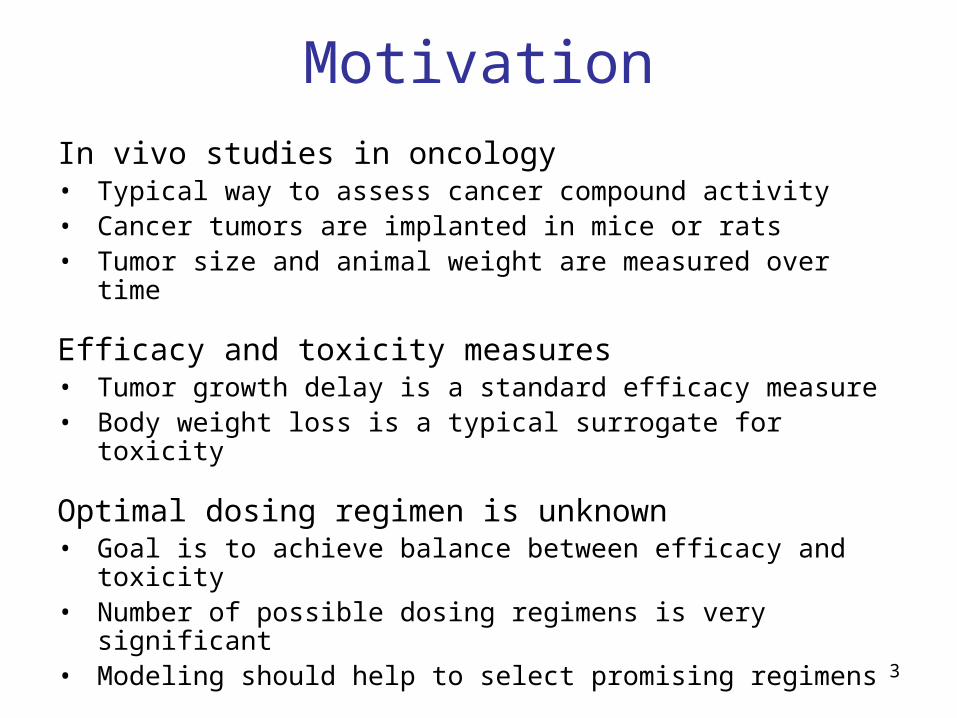
In vivo studies in oncology• Typical way to assess cancer compound activity• Cancer tumors are implanted in mice or rats• Tumor size and animal weight are measured over time

Efficacy and toxicity measures• Tumor growth delay is a standard efficacy measure• Body weight loss is a typical surrogate for toxicity

Optimal dosing regimen is unknown• Goal is to achieve balance between efficacy and toxicity• Number of possible dosing regimens is very significant• Modeling should help to select promising regimens

4

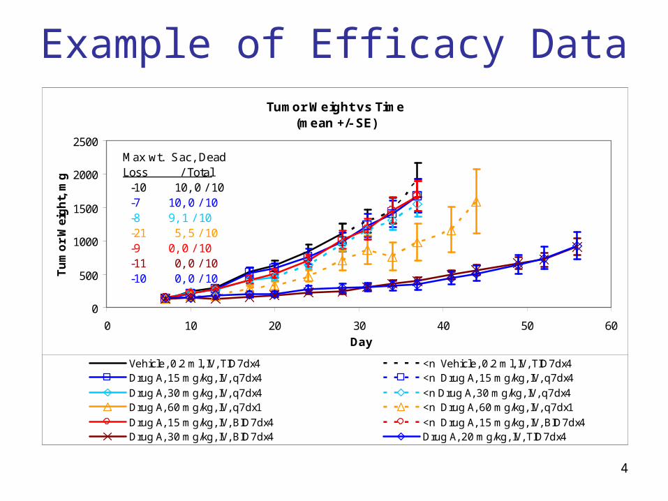
Example of Efficacy DataTumor Weight vs Time

(mean +/- SE)

0

500

1000

1500

2000

2500

0 10 20 30 40 50 60Day

Tu

mo

r W

eig

ht,

mg

Vehicle, 0.2 ml, IV, TID7dx4 <n Vehicle, 0.2 ml, IV, TID7dx4Drug A, 15 mg/kg, IV, q7dx4 <n Drug A, 15 mg/kg, IV, q7dx4

Drug A, 30 mg/kg, IV, q7dx4 <n Drug A, 30 mg/kg, IV, q7dx4Drug A, 60 mg/kg, IV, q7dx1 <n Drug A, 60 mg/kg, IV, q7dx1

Drug A, 15 mg/kg, IV, BID7dx4 <n Drug A, 15 mg/kg, IV, BID7dx4Drug A, 30 mg/kg, IV, BID7dx4 Drug A, 20 mg/kg, IV, TID7dx4

Max wt. Sac, DeadLoss / Total -10 10, 0 / 10 -7 10, 0 / 10 -8 9, 1 / 10 -21 5, 5 / 10 -9 0, 0 / 10 -11 0, 0 / 10 -10 0, 0 / 10

5

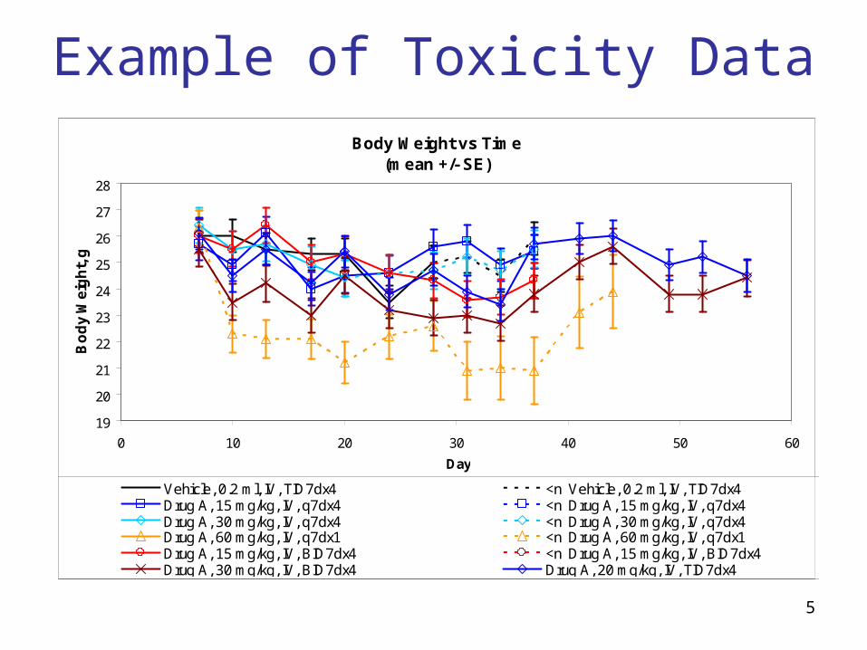
Example of Toxicity DataBody Weight vs Time

(mean +/- SE)

19

20

21

22

23

24

25

26

27

28

0 10 20 30 40 50 60

Day

Bo

dy

We

igh

t, g

Vehicle, 0.2 ml, IV, TID7dx4 <n Vehicle, 0.2 ml, IV, TID7dx4Drug A, 15 mg/kg, IV, q7dx4 <n Drug A, 15 mg/kg, IV, q7dx4Drug A, 30 mg/kg, IV, q7dx4 <n Drug A, 30 mg/kg, IV, q7dx4Drug A, 60 mg/kg, IV, q7dx1 <n Drug A, 60 mg/kg, IV, q7dx1Drug A, 15 mg/kg, IV, BID7dx4 <n Drug A, 15 mg/kg, IV, BID7dx4Drug A, 30 mg/kg, IV, BID7dx4 Drug A, 20 mg/kg, IV, TID7dx4

6

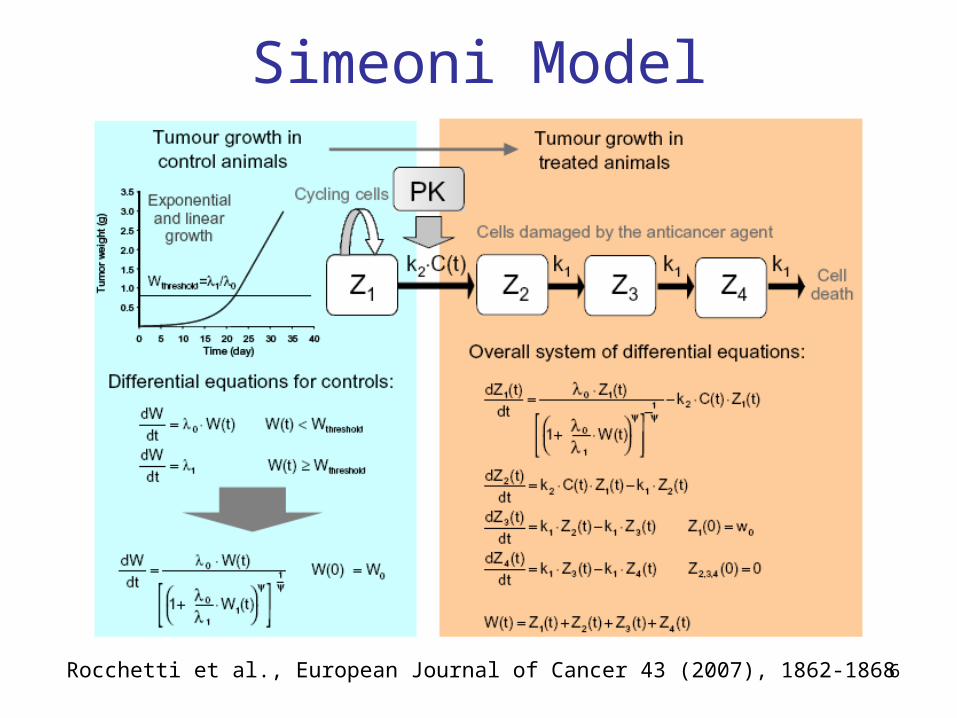
Simeoni Model

Rocchetti et al., European Journal of Cancer 43 (2007), 1862-1868

7

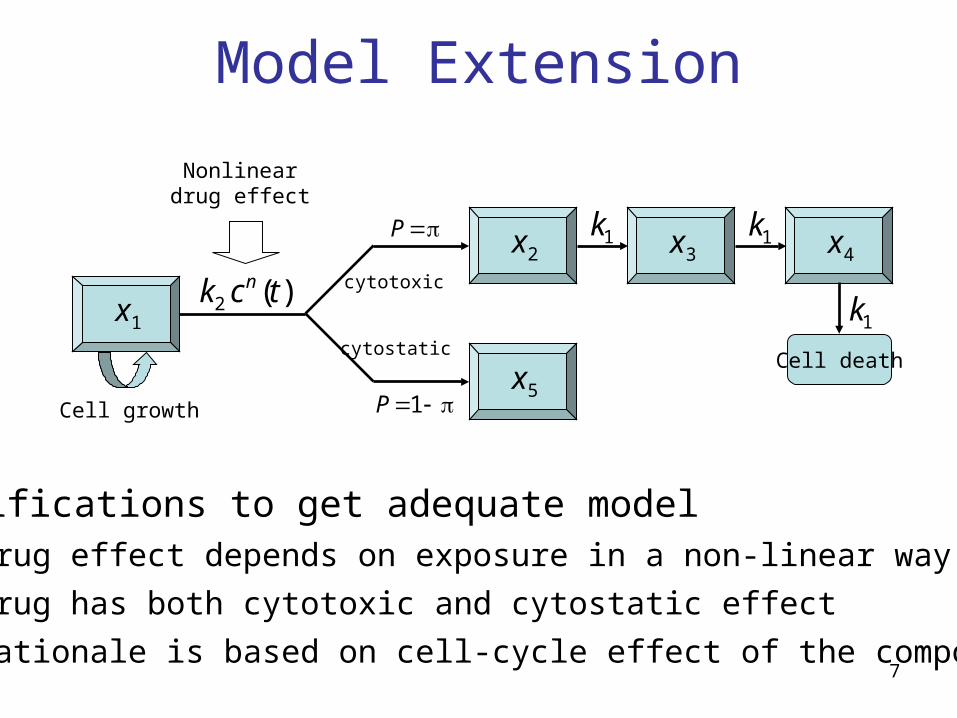
Model Extension

)(2 tck n

P

x1

x2

Nonlineardrug effect

1P

cytotoxic

cytostatic

x5

x3 x41k 1k

1k

Cell death

Modifications to get adequate model• Drug effect depends on exposure in a non-linear way

• Drug has both cytotoxic and cytostatic effect

• Rationale is based on cell-cycle effect of the compound

Cell growth

8

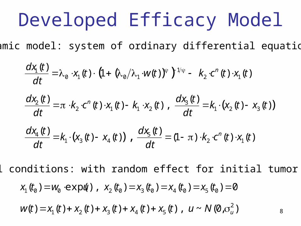
Developed Efficacy Model

)()()1()(

)()()(

)()()(

),()()()(

)()()(1)()(

125

4314

3213

21122

121

10101

),(

)(

)( )(

txtckdt

tdxtxtxk

dt

tdx

txtxkdt

tdxtxktxtck

dt

tdx

txtcktwtxdt

tdx

n

n

n

),0(~),()()()()()(

0)()()()(),exp()(

254321

05040302001

uNutxtxtxtxtxtw

txtxtxtxuwtx

Dynamic model: system of ordinary differential equations

Initial conditions: with random effect for initial tumor weight

90 10 20 30 40 50 60

-2.5

-2

-1.5

-1

-0.5

0

0.5

1

1.5

Time (days)

log(

Tum

or w

eigh

t)

0 10 20 30 40 50 60-2.5

-2

-1.5

-1

-0.5

0

0.5

1

Time (days)

log(

Tum

or w

eigh

t)

5 10 15 20 25 30 35 40-2.5

-2

-1.5

-1

-0.5

0

0.5

1

1.5

Time (days)

log(

Tum

or w

eigh

t)

5 10 15 20 25 30 35 40 45-2.5

-2

-1.5

-1

-0.5

0

0.5

1

Time (days)

log(

Tum

or w

eigh

t)

5 10 15 20 25 30 35 40-2.5

-2

-1.5

-1

-0.5

0

0.5

1

1.5

Time (days)

log(

Tum

or w

eigh

t)

5 10 15 20 25 30 35 40-2.5

-2

-1.5

-1

-0.5

0

0.5

1

1.5

Time (days)

log(

Tum

or w

eigh

t)

5 10 15 20 25 30 35 40-3

-2.5

-2

-1.5

-1

-0.5

0

0.5

1

1.5

2

Time (days)

log(

Tum

or w

eigh

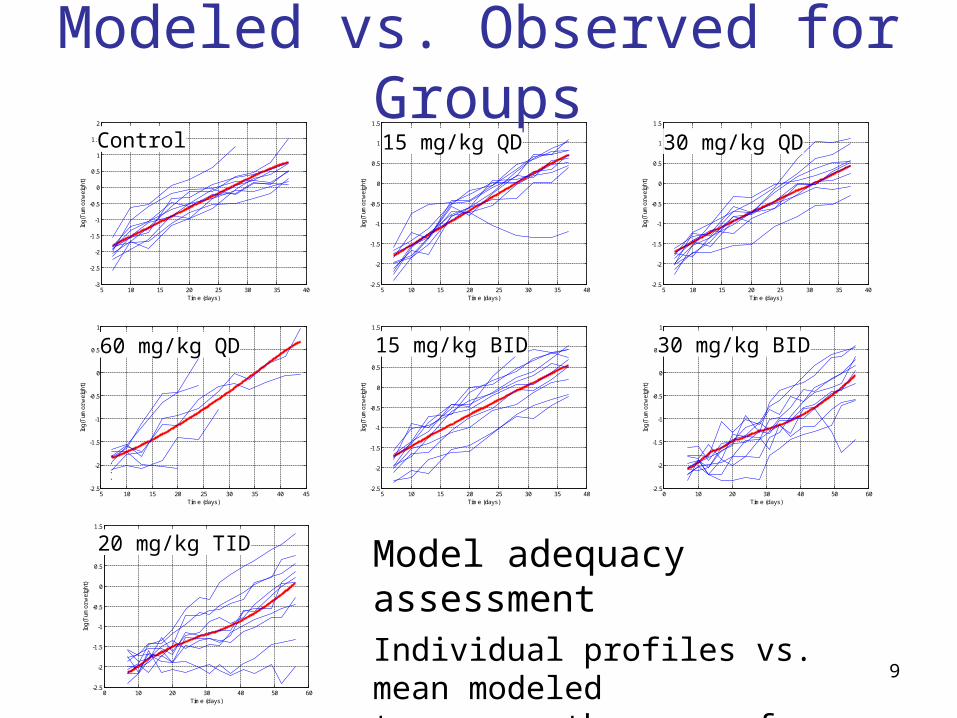
t)Modeled vs. Observed for Groups

Model adequacy assessmentIndividual profiles vs. mean modeled tumor growth curves for each group

Control 15 mg/kg QD 30 mg/kg QD

60 mg/kg QD 15 mg/kg BID 30 mg/kg BID

20 mg/kg TID

10

Efficacy Model Results

0 10 20 30 40 50 600

0.5

1

1.5

2

2.5

Time (days)

Tum

or

wei

ght

Control15 mg/kg q7dx4

30 mg/kg q7dx4

60 mg/kg q7dx1

15 mg/kg BID7dx4

30 mg/kg BID7dx420 mg/kg TID7dx4

Modeled population-average tumor growth curves for each dose group

115 10 15 20 25 30 35 40

0.96

0.965

0.97

0.975

0.98

0.985

0.99

0.995

1

1.005

1.01

Time (days)

Rel

ativ

e bo

dy w

eigh

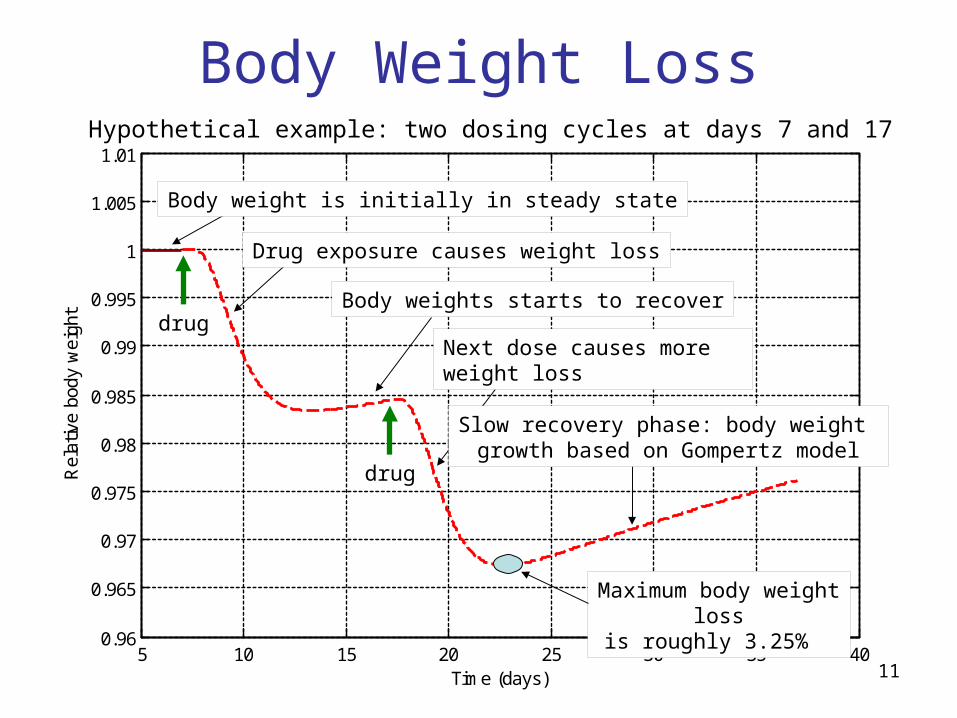
tBody Weight Loss

drug

drug

Hypothetical example: two dosing cycles at days 7 and 17

Body weight is initially in steady state

Drug exposure causes weight loss

Body weights starts to recover

Next dose causes more weight loss

Slow recovery phase: body weight growth based on Gompertz model

Maximum body weight lossis roughly 3.25%

12

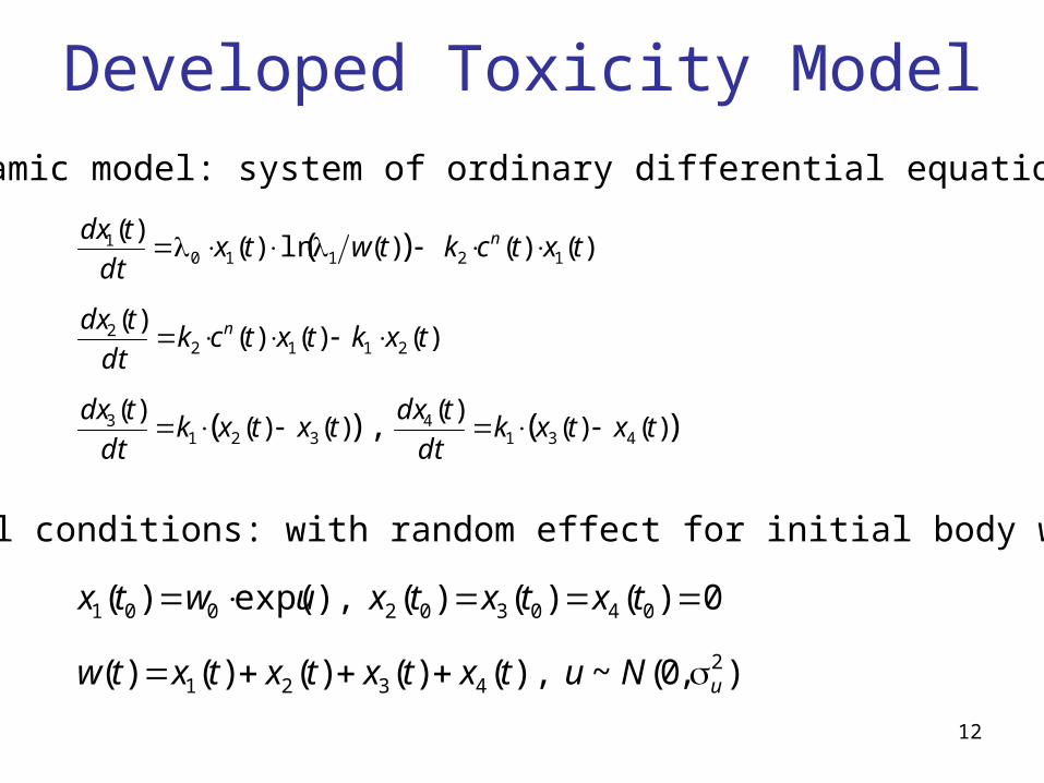
Developed Toxicity Model

)(),(

)(

)()()(

)()()(

)()()()(

)()()(ln)()(

4314

3213

21122

121101

txtxkdt

tdxtxtxk

dt

tdx

txktxtckdt

tdx

txtcktwtxdt

tdx

n

n

),0(~),()()()()(

0)()()(),exp()(

24321

040302001

uNutxtxtxtxtw

txtxtxuwtx

Dynamic model: system of ordinary differential equations

Initial conditions: with random effect for initial body weight

135 10 15 20 25 30 35 40

0.75

0.8

0.85

0.9

0.95

1

1.05

1.1

1.15

1.2

1.25

Time (days)

Rel

ativ

e bo

dy w

eigh

t

5 10 15 20 25 30 35 400.75

0.8

0.85

0.9

0.95

1

1.05

1.1

1.15

1.2

1.25

Time (days)

Rel

ativ

e bo

dy w

eigh

t

5 10 15 20 25 30 35 400.75

0.8

0.85

0.9

0.95

1

1.05

1.1

1.15

1.2

1.25

Time (days)

Rel

ativ

e bo

dy w

eigh

t

5 10 15 20 25 30 35 400.75

0.8

0.85

0.9

0.95

1

1.05

1.1

1.15

1.2

1.25

Time (days)

Rel

ativ

e bo

dy w

eigh

t

5 10 15 20 25 30 35 400.75

0.8

0.85

0.9

0.95

1

1.05

1.1

1.15

1.2

1.25

Time (days)

Rel

ativ

e bo

dy w

eigh

t

5 10 15 20 25 30 35 400.75

0.8

0.85

0.9

0.95

1

1.05

1.1

1.15

1.2

1.25

Time (days)

Rel

ativ

e bo

dy w

eigh

t

5 10 15 20 25 30 35 400.75

0.8

0.85

0.9

0.95

1

1.05

1.1

1.15

1.2

1.25

Time (days)

Rel

ativ

e bo

dy w

eigh

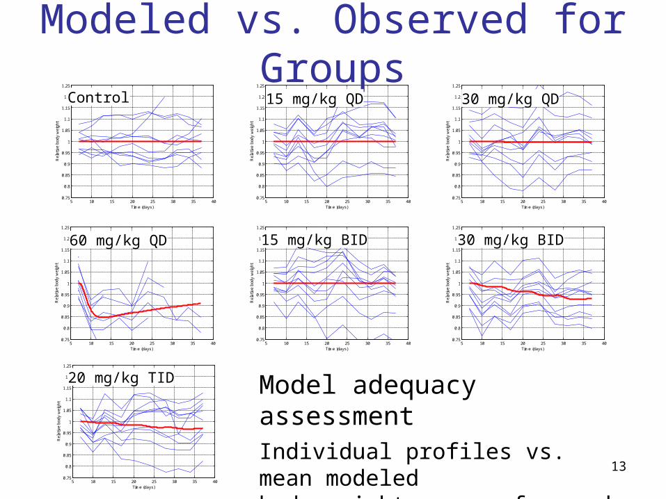
tModeled vs. Observed for Groups

Model adequacy assessmentIndividual profiles vs. mean modeled body weight curves for each group

Control 15 mg/kg QD 30 mg/kg QD

60 mg/kg QD 15 mg/kg BID 30 mg/kg BID

20 mg/kg TID

14

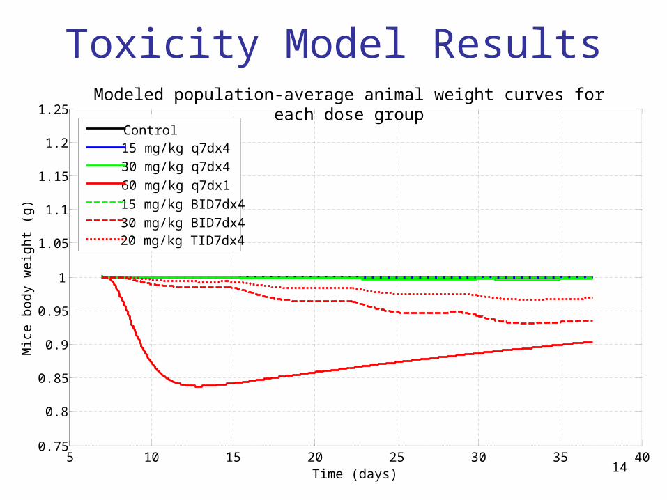
Toxicity Model Results

5 10 15 20 25 30 35 400.75

0.8

0.85

0.9

0.95

1

1.05

1.1

1.15

1.2

1.25

Time (days)

Mic

e b

ody

wei

ght

(g)

Control15 mg/kg q7dx4

30 mg/kg q7dx4

60 mg/kg q7dx1

15 mg/kg BID7dx4

30 mg/kg BID7dx420 mg/kg TID7dx4

Modeled population-average animal weight curves for each dose group

15

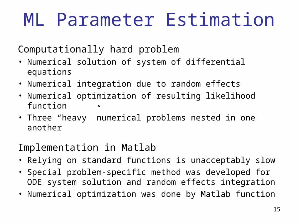
ML Parameter Estimation

Computationally hard problem• Numerical solution of system of differential equations• Numerical integration due to random effects• Numerical optimization of resulting likelihood function• Three “heavy ”numerical problems nested in one another

Implementation in Matlab• Relying on standard functions is unacceptably slow• Special problem-specific method was developed for ODE

system solution and random effects integration • Numerical optimization was done by Matlab function

16

Regimens Simulation

Simulation settings• Dosing was performed until day 28 as in original study

• Doses from 1 to 30 mg/kg (QD, BID, TID) were used

• Dosing interval was varied between 1 and 14 days

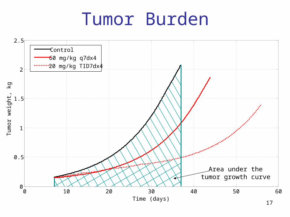
Regimen evaluation• Efficacy and toxicity were computed for each regimen

• Efficacy was defined as overall tumor burden reduction

• Toxicity was defined as maximum relative weight loss

• Efficacy was plotted vs. toxicity for each simulation run

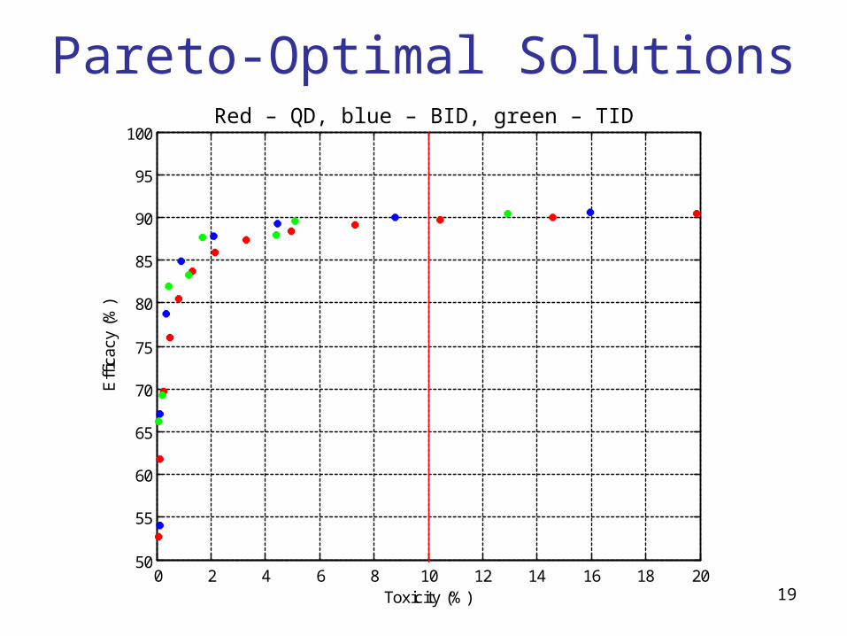
• Pareto-optimal solutions were identified for QD, BID, TID

17

Tumor Burden

0 10 20 30 40 50 600

0.5

1

1.5

2

2.5

Time (days)

Tum

or

wei

ght,

kg

Control

60 mg/kg q7dx4

20 mg/kg TID7dx4

Area under thetumor growth curve

18

Efficacy-Toxicity PlotRed – QD, blue – BID, green – TID

0 2 4 6 8 10 12 14 16 18 2050

55

60

65

70

75

80

85

90

95

100

30 mg/kg BID7dx4

20 mg/kg TID7dx4

Toxicity (%)

Eff

icac

y (%

)

19

Pareto-Optimal SolutionsRed – QD, blue – BID, green – TID

0 2 4 6 8 10 12 14 16 18 2050

55

60

65

70

75

80

85

90

95

100

Toxicity (%)

Eff

icac

y (%

)

200 2 4 6 8 10 12 14 16 18 20

50

55

60

65

70

75

80

85

90

95

100

Toxicity (%)

Eff

icac

y (%

)

Pareto-Optimal SolutionsRed – QD, blue – BID, green – TID

Zoomingthis part …

21

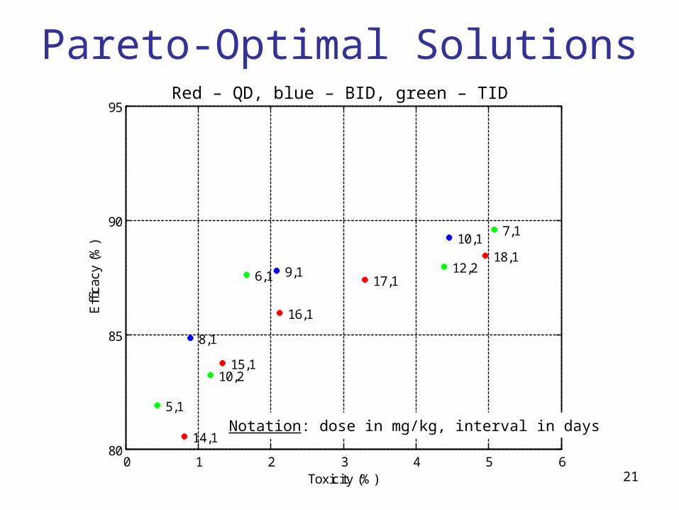
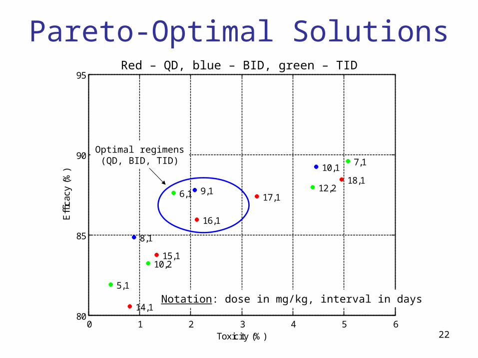
Pareto-Optimal SolutionsRed – QD, blue – BID, green – TID

0 1 2 3 4 5 680

85

90

95

14,1

15,1

16,1

17,1

18,1

8,1

9,1

10,1

5,1

6,1

7,1

10,2

12,2

Toxicity (%)

Eff

icac

y (%

)

Notation: dose in mg/kg, interval in days

220 1 2 3 4 5 6

80

85

90

95

14,1

15,1

16,1

17,1

18,1

8,1

9,1

10,1

5,1

6,1

7,1

10,2

12,2

Toxicity (%)

Eff

icac

y (%

)

Pareto-Optimal Solutions

Optimal regimens(QD, BID, TID)

Red – QD, blue – BID, green – TID

Notation: dose in mg/kg, interval in days

23

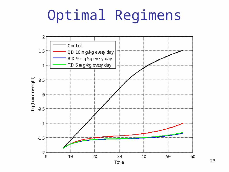
Optimal Regimens

0 10 20 30 40 50 60-2

-1.5

-1

-0.5

0

0.5

1

1.5

2

Time

log(

Tum

or w

eigh

t)

Control

QD 16 mg/kg every day

BID 9 mg/kg every day

TID 6 mg/kg every day

24

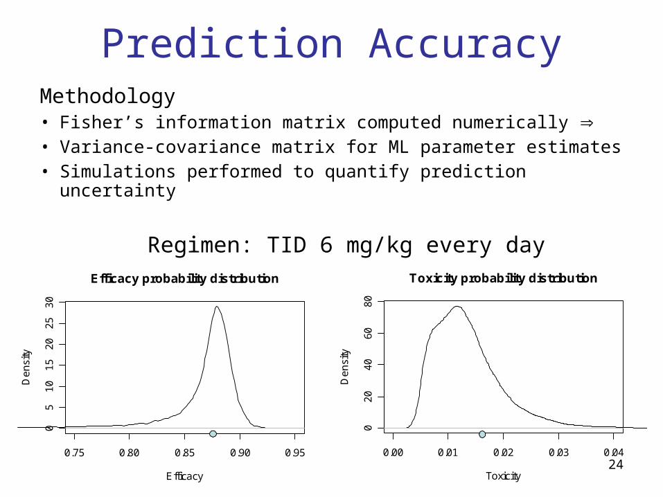
Prediction Accuracy

Regimen: TID 6 mg/kg every day

0.75 0.80 0.85 0.90 0.95

05

10

15

20

25

30

Efficacy probability distribution

Efficacy

De

nsi

ty

0.00 0.01 0.02 0.03 0.04

02

04

06

08

0

Toxicity probability distribution

Toxicity

De

nsi

ty

Methodology• Fisher’s information matrix computed numerically • Variance-covariance matrix for ML parameter estimates• Simulations performed to quantify prediction uncertainty

25

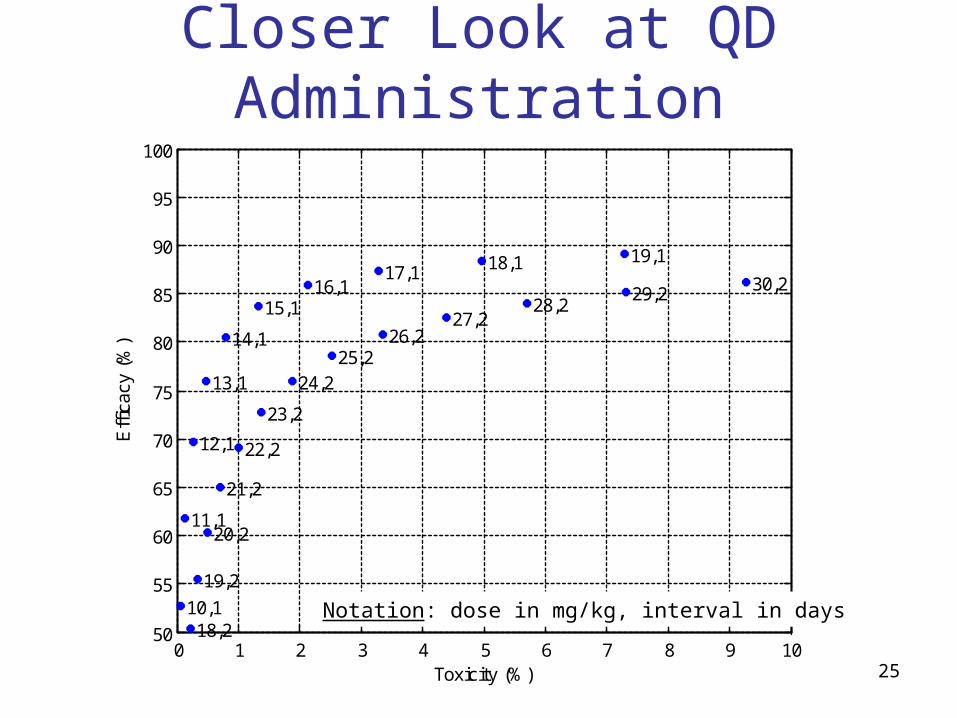
Closer Look at QD Administration

0 1 2 3 4 5 6 7 8 9 1050

55

60

65

70

75

80

85

90

95

100

10,1

11,1

12,1

13,1

14,1

15,1 16,1

17,1 18,1

18,2

19,1

19,2

20,2

21,2

22,2

23,2

24,2 25,2

26,2 27,2

28,2 29,2 30,2

Toxicity (%)

Eff

icac

y (%

)

Notation: dose in mg/kg, interval in days

26

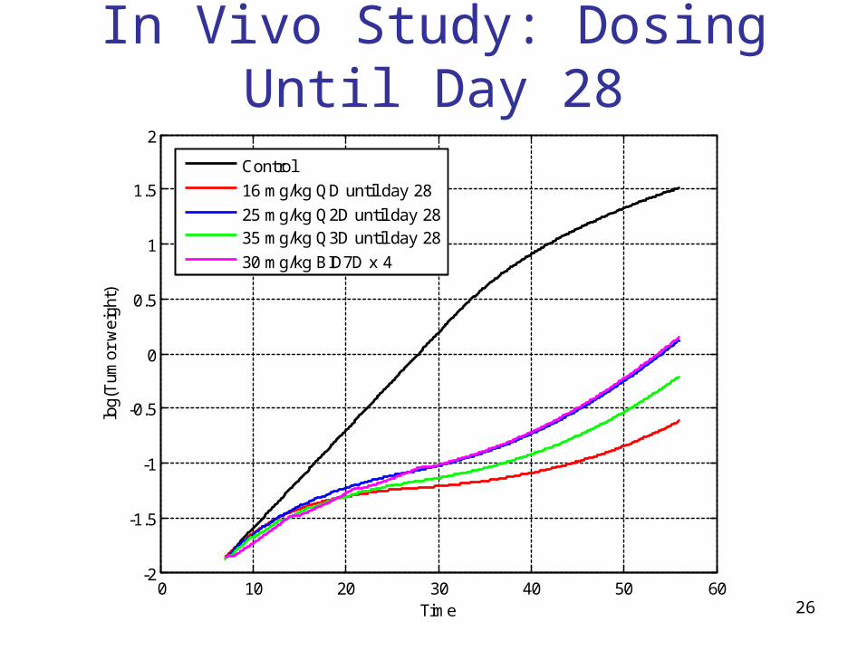
In Vivo Study: Dosing Until Day 28

0 10 20 30 40 50 60-2

-1.5

-1

-0.5

0

0.5

1

1.5

2

Time

log(

Tum

or w

eigh

t)

Control

16 mg/kg QD until day 28

25 mg/kg Q2D until day 2835 mg/kg Q3D until day 28

30 mg/kg BID7D x 4

27

Summary

Methodological contribution• New multiobjective method for optimal regimen selection• Novel dynamic model for cancer tumor growth inhibition• Novel dynamic model for animal body weight loss

Practical contribution• More efficacious and less toxic in vivo dosing regimens• Better understanding of compound potential pre-clinically

Validation• Application of modeling results to in vivo study in progress

28

Acknowledgements

Project collaborators

• Philip Iversen

• Harold Brooks

Data generation

• Robert Foreman

• Charles Spencer