RESOURCE MANAGEMENT IN CELLULAR COMMUNICATION NETWORKS WITH SUBSCRIBER PROFILE PREDICTION

A THESIS SUBMITTED TO THE GRADUATE SCHOOL OF NATURAL AND APPLIED SCIENCES

OF MIDDLE EAST TECHNICAL UNIVERSITY

BY

NUSRAT YILMAZ

IN PARTIAL FULFILLMENT OF THE REQUIREMENTS FOR

THE DEGREE OF DOCTOR OF PHILOSOPHY IN

ELECTRICAL AND ELECTRONIC ENGINEERING

JUNE 2005

Approval of the Graduate School of Natural and Applied Science

Prof. Dr. Canan Özgen Director

I certify that this thesis satisfies all the requirements as a thesis for the degree of Doctor of Philosophy.

Prof. Dr. İsmet Erkmen Head of Department

This is to certify that we have read this thesis and that in our opinion it is fully adequate, in scope and quality, as a thesis for the degree of Doctor of Philosophy.

Prof. Dr. Rüyal Ergül Supervisor

Examining Committee Members Prof. Dr. Yalçın Tanık (METU, EE) Prof. Dr. Ruyal Ergül (METU, EE) Prof. Dr. Mete Severcan (METU, EE) Dr. Ali Özgür Yılmaz (METU, EE) Prof. Dr. Erdal Arıkan (Bilkent, EE)

iii

I hereby declare that all information in this document has been obtained and presented in accordance with academic rules and ethical conduct. I also declare that, as required by these rules and conduct, I have fully cited and referenced all material and results that are not original to this work.

Name, Last name : Nusrat, Yılmaz

Signature :

iv

ABSTRACT

RESOURCE MANAGEMENT IN CELLULAR COMMUNICATION

NETWORKS WITH SUBSCRIBER PROFILE PREDICTION

YILMAZ, Nusrat

Ph.D., Department of Electrical and Electronics Engineering

Supervisor : Prof. Dr. Ruyal Ergül

June 2005, 168 pages

In this study, a dynamic resource management and subscriber profile prediction

scheme for mobile communication systems is presented. The aim is to achieve a

high level of QoS for both handoff calls and new calls, while at the same time to

improve the utilization of wireless network resources. The simultaneous

satisfaction of these two actually conflicting interests will be thanks to two major

key features. First, it will be due to the individual subscriber profile based prior

information about handoff reservation requests that are provided by the mobile

terminals. This information is based on the cell transition probabilities calculated

by the mobile itself using collected information during past operations. Second, it

will be due to a two-way approach implemented in the resource management

processes. The two-way approach controls both the amount of reserved radio

channels and the new call admission in a dynamic way, depending on the

subscriber mobility and network traffic conditions.

Keywords: QoS, Resource Management, Handoff Call Failure, New Call

Blocking, Spectral Efficiency

v

ÖZ

HUCRESEL ILETISIM AGLARINDA KULLANICI KISISEL BILGILERI

DESTEKLI TELSİZ KANAL YÖNETİMİ

YILMAZ, Nusrat

Doktora, Elektrik Elektronik Mühendisliği Bölümü

Tez Yöneticisi : Prof. Dr. Ruyal Ergul

Haziran 2005, 168 sayfa

Bu çalışma, telsiz iletişim ağlarında çağrı aktarma ve yeni çağrı kabul etme

işlemlerinde yüksek bir hizmet kalitesini hedeflerken aynı zamanda kısıtlı telsiz

kaynaklarının kullanım verimini artırmayı hedefleyen yeni bir yaklaşım

içermektedir. Bu her iki hedefin aynı anda gerçekleştirilmesi, iki ana yöntem ile

sağlanmaya çalışılmıştır. İlk olarak, hareketli kullanıcı terminallerinde tutulan

istatistik bilgileri sayesinde herhengi bir kullanıcının yol güzergahının önceden

belirlemesi ve bu şekilde kullanıcının geçeceği bir sonraki hücrede o kullanıcı için

kanal tahsisinin yapılması ilkesi. İkinci olarak, radyo kanalı yönetiminde iki

aşamalı bir yaklaşım kullanılması ilkesi. Bu iki aşamalı yaklaşımla, ortamdaki

kullanıcıların hareketlilik durumuna ve ağ içindeki trafik durumuna bağlı olarak

dinamik bir şekide, yeni cağrı başlatma ve geçiş yapan çağrı için rezervasyon ve

kabul işlemleri kontrol edilmektedir.

Anahtar Kelimeler: Servis Kalitesi, Kaynak Yönetimi, Geçiş Yapan Çağrı

Düşmesi, Yeni Çağrı Engelleme, Spektrum Verimliliği

vi

To My Parents and My Family

vii

ACKNOWLEDGMENTS

The author wishes to express his deepest gratitude to his advisor, Prof. Dr. Ruyal

Ergül, for his guidance, advice, criticism and encouragement and insight

throughout the research.

The author also would like to thank to, Prof. Dr. Erdal Arıkan and Prof. Dr.

Yalçın Tanık, for their suggestions and comments.

The technical assistance of Baki Kuran, and Ercan Yıldırım is gratefully

acknowledged.

viii

TABLE OF CONTENTS

PLAGIARISM........................................................................................................iii ABSTRACT……………………………………………………………………...iv ÖZ………………………………………………………………………………....v ACKNOWLEDGMENTS……………………………………………………….vii TABLE OF CONTENTS…………………………………………………….....viii CHAPTER 1. INTRODUCTION……………………………………………………………...1 2. THE PROPOSED METHOD…………………………………………………21

2.1 Subscriber Profile Prediction………………………………………21 2.2 Resource Reservation Process...…………………………………...28 2.3 New Call Admission process...…………………………………….31

3. OPERATIONAL FIELD DATA……………………………………………...35 4. PERFORMANCE ANALYSIS………………………………………….........38

4.1 Definition of Parameters…………………………………………...38 4.2 System Models…………………….……………………………….43 4.3 Software Simulation………………………………………………..48

5. RESULTS OF PERFORMANCE ANALYSIS ……………………………....54

5.1 Results of Numerical Analysis …………………………………….54 5.2 Results of Software Simulation …………………………………...80 5.3 Software Simulation under fixed Pf...……………………………...99 5.4 Comparison of Results of Numerical Analysis and Software Simulation ….………………………………….…………………106

ix

5.5 Cost Analysis………………… ………………………………….110 6. CONCLUSIONS.............................................................................................109 APPENDICES Appendix A.1: Operational Field Network Traffic Data.....................................113 Appendix A.2: Operational Field Handoff Traffic Data......................................120 Appendix A.3: Cell to Cell Handoff Report........................................................127 Appendix A.4: Cell Handover Type Report .......................................................128 Appendix A.5: Cell Handover Reason Report ....................................................130 Appendix A.6: Cell TCH Traffic Channel Report ..............................................132 Appendix B.1 NCR Source Code ........................................................................137

Appendix B.2 FCR Source Code ........................................................................141

Appendix B.3 DCR Source Code ........................................................................144

Appendix B.4 DRCM Source Code ....................................................................150

Appendix C Sample GPSS World Simulation Report ........................................155

Appendix D Cost Analysis Results......................................................................161

REFERENCES………………………………………………………………….162 VITA………...………………………………………………………………….164

1

CHAPTER I

INTRODUCTION

Next generation mobile communication networks will support high-speed

data applications and multimedia services in small cell-size based network

architectures. Small cell structures have many advantages. However, they require

frequent handoffs for the mobile user due to small cell radius. Handoffs use more

resources than a static user due to seamless handoff requirement. The quality of

service requirements makes it necessary to give priority to handoff calls to avoid

call dropping. Hence, the increased rate of handoff requests in the network

environment makes it very difficult for the network to simultaneously satisfy the

required Quality of Service (QoS) and effectively utilize the radio network

resources.

One of the most common approaches used to guarantee QoS while ensuring

high channel utilization is to use channel allocation. Efficient utilization of

resources can be obtained if and only if good strategies for channel reservation are

employed. This subject has been studied by many researchers and there are

several published work related to channel allocation. Their objective was to

efficiently manage radio channels in a mobile communication system while

reducing handoff failure probability.

Previous works on this subject can be group as a) Fixed Channel

Assignment (FCA), b) Dynamic Channel Assignment (DCA), or c) Hybrid

Channel Assignment (HCA) strategies for handoff calls. All of these approaches

assume that handoff call dropping is highly undesirable, and therefore they

attempt to reduce handoff call failures. Channel reservation schemes can reduce

handoff failures efficiently, so they have been a preferable choice among various

handoff prioritization schemes.

The number of handoff attempts in a cellular network varies according to

factors such as user behavior and network traffic conditions. Furthermore, it is a

time dependent variable, depending on day and time. Hence, fixed channel

2

reservation schemes efficiency is a time dependent function. It can be efficient

during certain time periods corresponding to low traffic and very inefficient

during time periods corresponding to heavy traffic.

Handoff attempts do not vary totally randomly and can be predicted using

some observations such as time, location and area dependence as well as the

traffic conditions in the cells in question. The user mobility, which is a parameter

which is strongly dependent on geographical location of cells, needs to be

included in these predictions if accurate results are pursued. The call parameters

such as call frequency, call duration and mobility of user can be summed up and

called user behavior.

Therefore, it is our conjecture that it possible to predict handoff attempts

based on call statistics of the cellular network. As an alternative to fixed channel

reservation, reservation can be done adaptively, depending on the changes in

network traffic conditions and user behavior. The success of adaptive resource

management depends very much on the accuracy of the information provided

about user behavior, changes in network traffic conditions and on the ability of the

resource management algorithm in adapting to those changes. It can be assumed

that computational complexity and other considerations that resource management

algorithms have to deal with can be handled by the network without causing extra

cost in the system.

Many approaches have been proposed in literature to guarantee fast and

smooth handoff with low probability of failure and low probability of new call

blocking which is required to satisfy a certain QoS level and at the same time to

utilize wireless channels as efficiently as possible. They focused on methods like

estimating the probability that a mobile terminal will be active in a particular cell

at future moments, signal-strength based next cell predictions, signal-strength

based handoff decision, user location tracking, signal-strength based handoff

prioritization and trajectory predictions. Details of some of the published methods

will be presented later in this section. There are several problems or difficulties

involved in the methods that have been examined so far. The problems can vary

from high computational complexity involved in trajectory predictions to

3

difficulties in next cell prediction based received pilot signal strength information.

In some cases, difficulties can not be surmounted and in others, they lead to

inaccurate results. Hence, it was believed that some new approaches were needed

to obtain significant improvements in adaptive channel reservation strategies.

In this study, a novel approach has been aimed which assumes that each

mobile can keep statistical information about its own activities. This information

could be shared with the network, enabling network to estimate handoff call

probability in a simple and efficient way. Hence, network is enabled to make

handoff reservations on per user basis. This is expected to produce very efficient

resource utilization since adaptation can be continuous, based on information

provided by individual mobiles. This is very different from standard estimation

procedures which are based on long term ensemble averages and fail to make

accurate estimations valid for short time periods.

The resource management algorithm proposed uses this information both in

the channel allocation process and in the new call admission process. The new call

admission process is the policy applied by the network to allow new calls

admitted by the system or rejected, depending on level of resources available. In

telephone network terminology, this is equivalent to delaying incoming calls by

sending a busy tone during congestion.

The statistical information kept by the mobile concerns the information

based on cells visited, time of visit, calls made, time and duration of calls. This

information can be utilized any time to accurately predict the probability that

mobile will visit one of the neighboring cells. The accuracy will be improved if

some position information in the present cell is also available. This probability

will be called cell transition probability. These transition probabilities can be used

to predict the next cell along the path of the mobile. Once the next cell is

determined, a handoff reservation request will be sent to that cell. It is obvious

that the network and the base station controllers involved in this process and they

are cooperating. It is further assumed that the mobile has enough computational

and storage resources to collect, store and evaluate the necessary information.

4

This is quite logical considering the capabilities of today’s cellular phones

marketed.

As a summary, it can be said that the determination of the most appropriate

number of channels reserved for handoffs should be based on the estimation of

handoff probabilities by individual users since networks are not capable of

predicting such probabilities on a per user basis. The only agent that can make this

prediction accurately is the mobile itself. Then, the network can collect such

information from all potential handoff candidates and can make an intelligent

planning of the network resources.

Remaining part of this section presents a summary of published work, their

main points, advantages and disadvantages.

One of the most common approaches to guarantee QoS while ensuring high

bandwidth utilization is using some bandwidth allocation strategies for handoff

calls. In [1] such a bandwidth allocation strategy for wireless ATM networks

using predictive reservation is proposed. The proposed approach is based on using

mobility patterns and reservation is made dynamically. Paper [1] focuses on

performance parameters such as new call blocking probability, handoff drooping

probability, and successful call termination probability and bandwidth utilization.

Most of the reservation algorithms proposed in literature make use of the

knowledge of mobility patterns (i.e. the probability that a mobile in cell i will

travel to cell j) to accurately perform the reservation. Paper [1] tries to predict the

mobility patterns by utilizing previous history information of the mobiles. The

prediction is then used to reserve bandwidth in the “next cell” in advance. This

paper assumes a micro-cell/pico-cell environment, such as WATM networks, in

which handoff rate is high. One has to consider the decision in which cell to

reserve bandwidth. In some previous studies it is propose to reserve bandwidth for

an ongoing call in all neighboring cells. This means of course waste of bandwidth

due to unnecessary reservation and thus an unnecessary increase in new call

blocking probability as well as a drop in bandwidth utilization. In [1], however

authors make use of the fact that mobile traffic does not move totally randomly,

instead it moves according to the presence of highways, streets, roads etc and thus

5

are somehow predictable. Therefore, it is possible to correctly predict the

movement of a mobile in a particular area with a high degree of accuracy, based

on the knowledge of previous history of the mobility patterns in the area. The

proposed scheme in [1] will predict the next cell a mobile will travel to, based on

the mobility information acquired from previous mobiles in the corresponding

area. However, the approach proposed in [1] doesn’t make any discrimination

between individual mobiles. Thus their approach is area or cell based.

Besides predicting the next cell based on mobility patterns, [1] proposes also

a new approach for the bandwidth reservation in the next cell, once the next cell

has been decided. At any time, the total capacity of a cell can be considered to be

composed of three parts: the used bandwidth (currently used by active mobiles),

the reserved bandwidth (reserved for future handoff calls) and the free bandwidth.

When a mobile tries to initiate a connection, it will be accepted if there is enough

bandwidth in the free bandwidth portion. When a mobile arrives from a neighbor

cell due to handoff, it is allowed to take bandwidth from reserved bandwidth

portion if there any amount of bandwidth reserved for it. Otherwise the handoff

connection will compete in the free bandwidth portion with the new call

connection attempts. There are several ways to reserve bandwidth in the

neighboring cells. In [1] the following reservation styles are studied and

compared: 1. Reservation in all surrounding cells, 2.Reserve in the neighbor with

the highest transition probability, 3. Reserve bandwidth according to the

respective value of the transition probability Pj for neighbor j, 5. Reserve in the

two neighbors with the highest transition probabilities.

The next generation mobile communication systems will introduce new

technologies and services including broadband communications and multi-

call/connection services. In [2], first the impact of these new technologies and

services on handoff performance is clarified. Then a new handoff method is

proposed in which the handoff connection setup is divided into the network

connection setup and the radio connection setup parts, with the former taking

place before a handoff request. The new network capabilities such as multi-

call/connection services and multimedia communications will seriously affect

handoff performance in mobile communications systems. The paper proposes a

6

new approach to resolve the handoff performance problem by trying to avoid

handoff failure in the next generation mobile communication systems.

When a handoff is required for a mobile terminal that communicates using

multi-call/connection services, it is required that all calls and connections are

handed over to the new cell in order to continue the service. This means that the

multi-call/connection handoff requires more processing than the conventional

single-call/connection handoff. In a small cell area handoff occurs more

frequently and the permissible handoff processing delay is less than in large cell

areas. These facts could result in situations in which the network cannot complete

the handoff before the deadline, which is when a mobile cannot communicate

with the old BS because of signal degradation. A handoff failure will then follow.

Authors in [2] propose some mechanism to support multi-call/connection service

handoffs in small cell areas while trying to utilize radio resources efficiently. The

main idea of the method proposed in [2] is to divide the network connection setup

process into the network connection setup part and the radio connection setup

part. The network connection is established before the handoff request is made

(referred to as “preprocessing”) based on pilot signal levels coming from the

surrounding cell. The network connection setup part is started when the difference

between the two signal levels (signal level of current BS and possible next BS)

falls below a threshold before the handoff request threshold is reached. In [2] it is

claimed that with the proposed way, switching the mobile’s radio channel from

old BS to new BS can be executed earlier than in the conventional method. Thus,

the handoff could be completed before the deadline even for a mobile moving

with a high speed in small cell areas.

The success of the proposed method in [2] depends very much on the correct

selection of the next radio cell since in this method the next cell is selected earlier

than in the conventional methods. Without going into details, in [2] some new

approaches for the next cell selection are addressed. These are, estimating the

signal level variations of the surrounding cells (and using this information in

obtaining the speed and direction of the mobile), using transportation information

(obtaining cell transition patterns based on map information present in network

database), using mobile patterns defined by user, using mobile patterns produced

7

by the network and using cell transition rate. None of these approaches are

detailed in [2] and need further study.

To efficiently handle radio channel reservation process in a mobile

communication system and reduce handoff failure probability, many studies are

performed using special handoff channels for handoff calls. In [3] a new class of

adaptive channel management schemes are proposed, aiming to reduce the

handoff failure probability below a predefined threshold by adjusting a channel

sharing ratio between new and handoff calls. In a resource-limited environment,

however, reducing the handoff failure probability increases the new call blocking

probability. The proposed schemes in [3] provide a flexible method to control the

desired QoS and to strike a balance between the “minimal” handoff failure

probability and the “minimal” new call blocking probability by controlling the

new call admission rate. The main approach of the schemes proposed in [3] is to

adaptively determine, based on current system load and the total number of

channels assigned to a cell, the “maximal” number of channels required to

guarantee that the handoff failure probability does not exceed a predefined

threshold. Two schemes are proposed which differ in the way they are dealing

with new calls. The first scheme, randomized Maximal Handoff Channel

Assignment Scheme (rMHCA), attempts to provide a better support for new calls

by allowing these calls to compete randomly with handoff calls for the remaining

channels after satisfying the level of QoS for handoff calls. The second scheme,

balanced Maximal Handoff Channel Assignment Scheme (bMHCA) dynamically

adjusts the new call admission rate to achieve a desired tradeoff between a

“minimal” handoff failure probability and a “ minimal” new call blocking

probability. However, since the number of handoff attempts varies according to

network conditions, fixed reservation schemes for handoff attempts can be

inefficient.

Since handoff attempts can be predicted using some observations such as

time dependence of handoff attempts and location or area dependence of handoff

attempts, it is possible to predict handoff attempts and to adaptively reserve

bandwidth according to these predictions. In [4] such an adaptive channel

reservation scheme is proposed to control the size of reservation capacity

8

according to the varying number of “soft handoff” attempts. “Soft handoff” is a

term defined and used in some papers like [4], to describe the condition where the

mobile finds a new BS with a pilot signal power higher than a predetermined

threshold, so that a new link is established to the new BS, while the old link to the

old BS is still kept. To maximize the system capacity or resource utilization, a

balancing procedure between soft handoff failure and new call blocking is also

proposed in [4]. In order to guarantee the QoS of soft handoff attempts, some

reservation capacity is required. However, a considerable amount of reserved

capacity can result in wasting the bandwidth, for a fixed value of the reservation

capacity, because the capacity required for soft handoff is time varying.

Therefore, in [4] a reservation method that adapts to the variations in the soft

handoff attempt rate is considered. The term “soft handoff” is also used in [4] to

represent the case where a mobile finds a neighboring cell with a received pilot

signal level higher than a predetermined threshold, TAdd. This is the “soft handoff

request threshold”, and thus a new link to the new BS is established while the old

link is still maintained. If the pilot-signal of either the link to the new BS or the

link to the old BS drops below a “drop” threshold, Tdrop, then the corresponding

link is released. One of the key points of [4] is the definition of a new threshold,

the “channel reservation request threshold”, TRsrv, which is lower than the

threshold for handoff request. If the mobile finds a BS with a received signal

higher than the channel reservation request threshold, then the mobile sends a

reservation request message to the associated Base Station Controller (BSC).

Afterwards, if the pilot strength drops and stays below the channel reservation

request threshold during a predetermined period of time, the mobile asks the

associated BSC to release the reserved capacity. On the other hand, if the signal

strength drops further and reaches the “drop threshold” then the mobile initiates

soft handoff using the reserved capacity. The “reservation threshold” is not an

absolute value but rather is a relative value to the soft handoff request threshold.

In [4] the handoff request threshold is dynamically determined according to the

current link status and thus the reservation request threshold also dynamically

determined guaranteeing adaptive channel reservation. This is illustrated in Fig 1,

9

which shows typical pilot strength variation as the mobile moves from one BS

area to another area.

Base Station A Base Station B

Figure 1. Reservation of channel capacity for soft handoff calls by a threshold

mechanism of pilot strength.

The reservation threshold must be adjusted carefully. It should be less than

the handoff request threshold so that the reserved capacity is available in the new

BS when the mobile actually requests the capacity for soft handoff. However, if it

is too low excessive unnecessary reservations can occur.

The proposed pilot-sensing reservation mechanism [4] will reduce

unnecessary blocking of new calls with priority on soft handoff calls. However,

system capacity also depends on the QoS service requirement difference between

new call blocking and soft handoff failures. A weighting factor is used due to the

higher relative importance of handoff calls over new calls. For a given weighting

factor, system capacity is determined mainly by the new call blocking

Reservation Request to

BS B

Soft Handoff

Initiation with

Reservation

Handoff Request

to BS B

T Add

T Rsrv

TDrop

Pilot Strength

10

requirement, if the new call blocking requirement is higher than the weighted soft

handoff failure probability requirement. On the other hand, if the weighted

handoff failure probability requirement is higher than the new call blocking

probability requirement, the excessive soft handoff failure probability requirement

limits the system capacity. Thus, the system capacity is maximal when the new

call blocking probability is equal to the weighted soft handoff failure probability.

Many studies use different approaches to keep a balance between the new

call blocking probability and the soft handoff failure probability. The approach

used in [4] is to control the size of minimum reservation capacity β0 , by counting

the numbers of new call blocking and soft handoff failures. A “moving window”

method is used to estimate the frequencies of new call blocking and handoff

failures. In this approach, in successive time intervals, the number of

successful/unsuccessful handoff calls and the number successful/unsuccessful

new calls are counted and the minimum reservation capacity β0 is determined

accordingly. However, the difficulty in the method proposed in [4] is in selecting

a proper size for the window-monitoring interval. Since the offered traffic is time-

varying, a short interval may not support a sufficient estimation for determining

the size of reservation capacity. On the other hand, the dynamic variation of the

offered traffic makes the reservation process inefficient if the monitoring interval

is too long.

User mobility profile prediction, i.e. predicting the probabilities that a

mobile will be active in other cells in future moments, has gained considerable

attention in the field of wireless communications. This information can be

valuable for the successful handoff process, especially in those approaches, which

use prior channel reservation for handoff calls. The prediction information can be

used to assist the BS to maintain a balance between guaranteeing quality of

service (QoS) to mobile users and achieving maximum resource utilization. In [5],

a novel adaptive fuzzy logic inference system to estimate and predict the

probability information for direct sequence code division multiple access

DS/CDMA wireless communication networks is proposed. The estimation is

based on measured pilot signal strength received by the mobile from a number of

11

nearby BS and the prediction is obtained using the recursive least square (RLS)

algorithm.

Previous research efforts in this field are mainly focused on statistics such as

user location tracking [17], trajectory prediction, channel holding time, cell

boundary crossing rate, mean handoff rate and cell residence time. What is

different in [5] is that, the authors are more interested in the probabilities that a

mobile user will be active in a particular cell at a future moment.

In general, if a mobile user is closer to a BS, then the propagation path

attenuation from the mobile user to the BS is smaller and vice versa. Therefore, if

the BS transmits a pilot signal with constant transmitted power then the received

signal power at the mobile user carries the information about the distance between

the mobile user and the BS. Since the probability that a mobile user will be active

in a particular cell at a future moment is a function of the current distance between

the mobile and its nearby base stations, the probability can be estimated based on

real-time measurements of the received pilot signal power at the mobile.

Moreover, the probability depends also on the mobile movement pattern

(movement trajectory) since the movement of each mobile has a smooth trajectory

most of the time. So, the location of a mobile user at a future moment depends on

its location at the current moment as well as previous moments. Making use of

these two facts, in [5] it is considered that it is possible to predict the mobility

information of a mobile, based on the current and previous measurements of

signal strength.

In [5], some important facts about the signal strength measurement

technique are pointed out, which are not addressed in papers based on signal

strength calculations [1, 2, 4, 9, 16, 20] that use a similar approach in estimating

and predicting the next cell. There are some challenges in estimating and

predicting the mobility information based on just the pilot signal power

measurements because of a couple of facts. Normally there is no one-to-one

relationship between the distance and probability. Even if such a relationship

would exist, it is very difficult if not impossible to describe such a relationship

accurately using mathematical expressions. There are fluctuations in the received

12

signal level due to physical obstacles blocking the transmission path between the

BS and the mobile user. Shadowing randomizes the relationship between the

received pilot signal power, and the distance between the mobile and the BS.

In [19], the sources of received signal strength variation are addressed.

These are, change in mean strength due to changing distance from the antenna,

rapid variation due to constructive and destructive interference of signals arriving

via different paths to the phone (fast fading), and slower variation due to

obstructions (shadow fading). A simple model of the effect of temporal variation

in signal strength on active-set membership, is developed in [19] for cellular

phone systems that use the soft-handoff algorithm. This model is based on a

steady state calculation.

The received signals are distorted by interference due to multiple users and

due to background noise. Therefore the measured data are not absolutely accurate.

Despite of these disadvantages, in [5] the signal strength measurement approach is

still used in estimating and predicting the next cell. However, to handle the

difficulty, in [5] an adaptive fuzzy inference system is proposed. The proposed

approach deals with the uncertainty inherent in the relation between the distance

and the probability, the random shadowing effect by using training data from real

measurement or statistical models of practical propagation environments.

To handle the measurement error, the system incorporates the degree of

certainty (or accuracy) of measurements by giving a larger degree of importance

to the data with higher measurement accuracy. The main concern of [5] is to

predict the mobility information of future moments with an adaptive fuzzy

inference approach to eliminate the difficulties that arise due to using only signal

strength information in determining the possible next cell. However, there some

open discussion points about the method proposed in [5]. For example, the

complexity of the fuzzy inference system may be a concern, especially when the

prediction accuracy is wanted to be high. The increased implementation

complexity makes the proposed system impractical for real-time application,

which is, of course, not good for next generation mobile communication systems.

13

Similarly, in [21] fuzzy logic theory and neural networks are used. The

intelligent call admission controller (ICAC) proposed in [21] contains a fuzzy call

admission processor to make admission decision for a call request by considering

QoS measures such as the forced termination (drop call) probability of handoff,

the outage probability of all service types, the predicted next-step existing-call

interference, the link gain, and the estimated equivalent interference of the call

request. Also, the pipeline recurrent neural network (PRNN) is used to accurately

predict the next-step existing-call interference, and the fuzzy logic theory is

applied to estimate the new/handoff call interference based on knowledge of

effective bandwidth method.

Approaches which reserves fixed amount of bandwidth (fixed number of

channels) for handoff calls, cannot adapt to changes in the network conditions.

This is clearly not suitable in the presence of burst data and emerging multimedia

traffic. Therefore, an adaptive and dynamic bandwidth allocation scheme is

essential in ensuring the QoS required. Several research studies are performed in

the field of adaptive channel allocation. Many of the proposed dynamic bandwidth

allocation alternatives involve heavy computational and signaling complexity due

to updates in system status, or require complex topology processing [24] for next

cell prediction, and information exchange between cells thus making them

difficult to be used in actual deployment.

The alternative proposed in [6] as an adaptive and dynamic channel

allocation scheme tries to overcome these deficiencies. The main features of [6]

are: The estimation is done on-line and periodically, hence it can effectively adapt

to changing traffic conditions, which is particularly suitable for multimedia type

of services. Bandwidth allocation is implemented by a probabilistic mechanism,

which can reserve the bandwidth in an efficient statistical manner. This eliminates

the need for reserving bandwidth explicitly for each call setup. The power of this

approach is in this periodic and on-line estimation, and in the statistical bandwidth

reservation mechanism.

The on-line estimation algorithm of [6] aims to reduce signaling load

required in most dynamic call admission algorithms. For example, some

14

approaches require that a cell has to obtain status information, such as channel

occupancy and traffic arrival rate, from all cells that have potential handoffs at the

beginning of a control period. This requires a significant amount of signaling. To

overcome this limitation, an on-line estimation algorithm is implemented, which

restricts the use of actual information to those only from the local cell, while the

statuses of the neighboring cells are derived by estimation rather than actual

signaling.

The adaptive bandwidth allocation algorithm of [6] is executed in a

distributed and periodic fashion, each cell executing identical algorithm based on

local estimations. At the beginning of a control period, the bandwidth allocation

algorithm determines the amount of bandwidth reserved in the next control period

for the particular cell by taking the traffic conditions into consideration. So, the

bandwidth reservation is done for all potential handoffs in a control period,

eliminating the need for reserving bandwidth for each call. This enables a more

efficient statistical multiplexing approach leading to a more efficient usage of the

bandwidth.

In [7], another way of dynamic channel reservation scheme is proposed to

improve the utilization of wireless network resources while trying to guarantee the

required QoS for handoff calls. The wireless channels are dynamically reserved

by using the “request probability” determined by the mobility characteristics and

“channel occupancy” to guarantee acceptable quality of handoff calls and keep the

new call blocking probability as low as possible.

In [7], it is pointed out that handoff will occur more frequently in next

generation mobile communication networks because the cell size is much smaller

to support high capacity on the limited radio spectrum. As the handoff rate

increases, bandwidth management and traffic control strategy, that is, call

admission control, handoff procedure etc., become more challenging problems.

Dropping probability of handoff calls and blocking probability of new calls are

considered also in [7] as critical QoS parameters. From the subscriber’s point of

view, forced termination due to handoff failure is considered to be less desirable

than blocking out a new call. Therefore, just like many other dynamic channel

15

reservation schemes, in [7] it is proposed to guarantee a QoS for handoff calls

while allowing a high utilization of wireless bandwidth. The paper [7] describes

two of the generic handoff prioritization schemes, among many channel allocation

schemes, as recent intensive research areas on channel allocation, namely the

queuing handoff request and reserving a number of channels exclusively for

handoff requests. In general, handoff prioritization schemes result in decreased

handoff failures and increased call blocking, which in turn, reduces total admitted

traffic.

In the handoff queuing scheme (HQS), it is assumed that there is a time

interval where the mobile spends some time in the handoff area. Thus, queuing of

the handoff request is possible, where it is physically capable of communicating

with both the current and the next BS. The fact that successful handoff can take

place anywhere during this time interval makes a certain amount of tolerance in

the delay for the actual channel assignment to the handoff request. New calls,

which originate within the cell, are blocked if all wireless channels are occupied

and are served only when a wireless channel is available and no handoff request

exists in the queue. Obviously, HQS can reduce the probability of forced

termination (so called in [7], other papers usually call this handoff failure),

however causes increased call-blocking probability. The reason is that no new call

is granted a wireless channel until all the handoff requests in the queue are served.

Another priority scheme is the fixed guard channel schemes (GCS), which

gives higher priority to handoff calls by assigning them a higher capacity limit, to

reduce the forced termination probability. Fixed GCS shares normal channels

between handoff and new calls, and reserves exclusively some guard channels for

handoff calls. Because fixed GCS is developed under stationary call arrival

assumption, it causes a reduction in the total carried traffic under non-stationary

traffic patterns due to fluctuation in the mobility.

The approaches studied from [1] to [6], do not take into account the

characteristics of network traffic and user mobility. In [7] a dynamic channel

reservation scheme (DCRS) is presented to guarantee the required dropping

probability of handoff calls while keeping the blocking probability as low as

16

possible. The key point in [7] is that, although the proposed method shares normal

channels between new calls and handoff calls, and reserves guard channels for

handoff calls, just like GCS, the guard channels reserved for handoff calls can

also be used for new calls depending on network status and mobility of calls. The

paper [7] defines a request probability that is used to allocate guard channels to

new calls. This request probability of new calls is adaptively determined

according to the mobility of calls, total number of channels in a cell, threshold

between normal channels and guard channels, and current number of used

channels. The flow diagram of call processing for the DCRS scheme is illustrated

in Fig.2.

Figure 2. Call processing flow diagram for DCRS

Handoff

Call

Channel

Available?

Yes Channel

Allocation

Ongoing

Call Channel

Release

Call

Dropping

No

New Call

Channel

Available?

System State

lower than

threhold?

Yes Yes Channel Allocation

Ongoing

Call

Channel

Release Call

Blocking Probability

Generator

No No

Request Probability (1-Request

Probability)

17

As stated before, the current trend in cellular communication networks is to

shrink cell size to accommodate more mobile users in a given area. This results in

more frequent handoffs, and makes connection level QoS more difficult to

achieve. The important connection-level QoS parameters are the probability of

blocking newly requested connections and the probability of dropping handoff

calls because of unavailability of channels in the new cell.

Since it is practically impossible to completely eliminate handoff drops, the

best one can do is to provide some form of probabilistic QoS guarantees. Several

studies have been performed in this field. In [8], five different recent schemes for

reserving bandwidth for handoff calls and admission control for new calls are

compared.

First two schemes compared in [8] are based on the estimation of handoffs

that may occur during a specific time window. In the first scheme, which is

referred as CHOI (after the name of the developer), the BS of a cell calculates the

required bandwidth to be reserved for anticipated handoffs form adjacent cells

upon arrival of a new connection request. The mobility, which is the handoff

behavior, of each user is estimated using a history of handoffs observed in each

cell. In the second scheme, referred to as NAG (distributed admission control), the

BS not only considers incoming handoff from adjacent cells, but also outgoing

handoffs to adjacent cells. The BS then calculates the total required bandwidth in

its cell for both handed off and existing connections. These schemes were

evaluated based on (1) an exponentially distributed time each mobile stays in a

cell; (2) the perfect knowledge about the mobility and lifetime of each user

connection. However, these two assumptions do not hold in reality.

The third considered scheme is an admission control scheme, referred to as

AG (Absolute Guarantee), which guarantees no handoff drop for any existing

connection. In the first two approaches it is not possible to eliminate completely

handoff call drops. AG on the other hand eliminates totally handoff failure. “No

handoff drop” can be achieved by checking bandwidth availability and reserving

bandwidth in all cells the mobile requesting a new connection is to traverse in

18

future. It is practically impossible to know all these cells in advance during the

call admission phase. In [8], it is shown how costly it is to make the handoff drop

probability zero even under the impractical assumption that all the cells that a

mobile will visit are known during call admission.

The fourth admission control scheme, known as BHARG (Per connection

reservation in next cell after admission), is based on per connection bandwidth

reservation. Unlike the first three approaches, this scheme predicts the next cell

the mobile will move into and the mobile’s per connection bandwidth is reserved

in that cell.

The last admission control scheme, referred to as NCBF (Next Cell

Bandwidth Reservation First), is similar to BHARG. In this scheme, both the

current cell and the predicted next cell along the path of the mobile that is

requesting a new connection should have enough bandwidth to accept the request

whereas BHARG requires that only the current cell has enough bandwidth. In [8],

it is shown that NCBF and BHARG are still costly compared to the first two

approaches.

The approaches compared in [8] use mobility estimation based on history of

handoffs observed in each cell. However, in predicting the next cell, only a single

previous cell is considered.

In [9], a different approach is presented for the handoff problem in wireless

networks. Signal strength and next cell prediction techniques are combined to

eliminate unnecessary handoffs and reduce the mean number of handoffs in dense

urban areas.

Small cell size, like in micro-cell and pico-cell environments, results in more

boundary crossings for the mobile, which in turn results in increased number of

handoffs between base stations. This, of course, increases the network load and

under heavy traffic conditions could cause the call to be dropped. In [9], the

starting point is the following fact: If it were possible to determine a candidate BS

in advance and then predict the signal strength values from this BS to the mobile,

a considerable reduction in mean number handoffs could be achieved. Signal

Strength prediction and Next-Cell prediction techniques are used in [9] to

19

determine this next BS correctly in advance. In the proposed approach, the

number of handoffs to each BS is recorded and updated recursively. This has the

effect of increasing the handoff weight to each BS, a measure that can be used to

prioritize and select a Most Likely Cell (MLC). Signal strength estimates from

this cell can then be obtained, which are used to predict critical handoff instants.

For the next-cell prediction, [9] uses an approach used in some previous

studies. Their approach is to predict the next visited cell, based on history of

handoffs of users and cells. These histories are aggregated in a profile server into

mobility profiles, which subsequently are expected to reflect the mobility pattern.

These are then used in the prediction process. The network is partitioned into

zones, with each zone including a profile server. The profile server and BS

exchange control messages to build handoff histories of users and cells. The BS

has the task of selecting the next-cell for the handoff user.

Once the next cell is found, signal strength estimates will be obtained and

utilized to predict the handoff request time instant. The received signal strength

from BS on the down link decays exponentially and slow fading associated with

this signal strength being highly correlated can be predicted easily. This

information is then used to predict the instant of handoff request. It is shown that

such a signal strength prediction method can eliminate unnecessary handoffs and

in this way can reduce mean number of handoffs. The success of the approach

proposed in [9] depends on the order of the predictor. Higher order predictors can

detect even deep fades and prevent unnecessary handoff requests under such deep

fading cases, at the expense of increased computational complexity.

There are many other working areas dealing with other aspects of the

handoff process or handoff procedures in wireless communication systems. These

can be grouped as wire-line resource management studies, wire-line bandwidth

allocation schemes, call admission control for QoS provisioning, path rerouting,

path extension and route optimization upon handoff, guaranteeing loss-less or

minimum delay (low latency) handoff, traffic modeling etc. Details of these other

areas will not be considered during this study.

20

However, it is important to point out that new and innovative approaches are

needed in order to improve channel utilization in networks where cell sizes are

small and there are considerable amount of cell boundary crossings due to high

mobility of users. These can be classified as 1- Better estimation of user behavior,

2- improved estimation of user position and user movements. The former requires

cooperation of individual mobiles since only the mobile can provide detailed

statistical data. The latter implies incorporation of GPS type of capabilities in

mobile devices which can provide better information on user position and

movements then signal strength measurements or other similar techniques.

21

CHAPTER II

THE PROPOSED METHOD

As explained in the introduction, new approaches are needed in resource

allocation in cellular networks. A novel approach, which employs statistical

information collected by mobile terminals, is explained in detail in this chapter. It

is presented in three sections. Section 2.1 describes the details of subscriber

profile prediction and in section 2.2; details of resource reservation process are

presented. Finally, in section 2.3, details of the new call admission process is

presented.

2.1 Subscriber Profile Prediction

Previous research effort on mobility information have focused on methods

like the probability that a mobile terminal will be active in a particular cell at

future moments [5], signal-strength based next cell prediction [4], signal-strength

based handoff decision algorithm [20], mobility model [3], user location tracking

[17], signal-strength based handoff prioritization [16], and trajectory prediction [2,

22]. All these methods depend mainly on the strength of the pilot signal received

by the mobile. Relying just on received pilot signal strength alone cannot provide

reliable information about the next cell to be visited. Furthermore, it gives no

information about the possibility of call termination before a possible handoff.

Depending on several factors like the individual user, called party, service type

and cell size, the call may or may not have a high handoff probability before

reaching the cell boundary. An illustrative example is the case of mobile from a

small town with an active voice call and a mobile along a highway with an active

high-speed data application. The mobile on the highway will have high handover

probability and possible over several cells whereas a mobile from the small town

will have a very small handover probability. To overcome such difficulties, it is

proposed that each mobile keeps mobility statistics (that is, cells visited, time of

visit, called subscriber and service specific average call durations, call elapsed

22

time for the active call, average distance traveled, average speed etc. Based on this

information, the cell transition probabilities, and thus prediction of next cell to be

visited, could be obtained for each mobile in a more accurate way.

One way to obtain cell transition probabilities is the following approach.

Let Ci denote the cell that the mobile is currently in. Next, the mobile will visit

one of the neighbors of Ci. This cell will belong to the set C, where C is the set of

all cells visited before and their neighboring cells. Each mobile keeps track of the

frequently visited cells in order to avoid C becoming excessively large. Hence, a

first time visited cell will be put on a temporary list and if not visited again within

a certain time, will be deleted from the list. For each of the cells frequently

visited, the mobile keeps transition probabilities form the current cell Ci to the cell

Cj, where Cj ε CK, where C

K ε C is the set of all neighboring cells of Ci. When

being in cell Ci, the mobile will pass to one of the K neighbors of cell Ci. Thus,

K

Σ Pik = 1 (1)

k=1

In Fig 3, the probability of transition for a mobile, from cell Ci to its

neighbor Ci2 (which is the second neighbor, k=2 among K=6 neighbors) is

illustrated.

Figure 3. Transition probabilities in a hexagonal cell structure.

P2 C

i

m .

Ci

C i 1

C i 2 C i 6

C i 5 C i 3

C i 4

Pi2

23

These probabilities can be represented as a probability array, defined over

the subset of neighbors. Let

P C i = {Pi1, Pi2 ... PiK} (2)

denote the transition probabilities of the mobile visiting a certain cell Ci. Here, K

is the maximum number of neighbors. Hence, each mobile will be required to

store a K x M matrix, where M is the number of frequently visited cells. This

matrix is defined as the transition probability matrix; Hm. Hm is the “Mobility

State” of the mobile. Therefore;

Hm = {PC0, P

C1, P

C2, … , P

CM-1, P

CM }

T (3)

Entries of the Cell Transition Probability Matrix are the cell transition

probabilities Pij, which represent the probability of a transition from cell i to cell j.

Pij, represents the probability of passing to cell j when being in cell Ci. Therefore,

with each cell transition the mobile derives Pij and puts it into the corresponding

fields of Hm. To derive Pij, the mobile keeps counters Ni for each cell Ci, and

counters Tij for each cell pair Cij. The mobile will increment the counter Ni, with

each visit to cell Ci, and will increment Tij for each transition from cell Ci to Cj.

The Pij is then derived as:

Pij = (total transitions from Ci to Cj) / (total visits to Ci)

Pij = (Ni / Tij) (4)

It is important to develop a policy for which cells to keep mobility statistics,

which cells to ignore, when and how to reset counters. We propose to ignore all

cells, which are not visited at least 3 times during a certain time period, say six

months. Moreover, all entries will be kept in FIFO type data structures, to ensure

that older transitions are deleted automatically as newer ones are added to the

statistics.

By keeping track of the cell transitions, each MT “learns” actually its own

mobility pattern. In this aspect, this method is also suitable for a neural network

24

implementation approach and provides more accurate information about the

mobility of each individual mobile.

It was demonstrated by simple calculations that, storing mobility statistics

and transition probability information does not take much of the resources

available in today’s mobile terminals, i.e. hand held devices. Therefore, mobile

terminals are assumed to have enough resources to handle these calculations.

When entering a new cell, the mobile will inform the new cell, via the

signaling channel, about the cell transition probabilities, by transferring the

corresponding row of the mobility state Hm to the BS of the current cell. It is just a

simple array of data that is sent to the BS of the current cell, in order to inform it

about the intent of the corresponding mobile to visit which cell next. No much

signaling or computational complexity is involved in this process, and is very

simple compared to the methods that were examined so far.

In this way, the mobile informs the BS of the new cell, which cell or cells

and with which probabilities it will most likely visit after this current cell. The BS

of the current cell will then use this information together with others, to decide on

the next cell, and to decide whether to make a reservation request to the

corresponding neighboring cell or not. When the mobile leaves a cell Hm must be

updated accordingly, to reflect the latest transition. The mobile will increment the

corresponding counters and update Hm when making a new transition.

Depending on the relative magnitudes of the transition probabilities Pij, the

BS of the current cell Ci can request reservation in more than one cell to improve

handoff success probability and thus reduce handoff failure probability. Paper [1]

compares different approaches in reserving BW in one or more than one cell to

increase success probability. In [1], it was shown that making reservation requests

only in the highest probable neighboring cell, compared to other methods, like

reserve-uniform or reserve-max2, results in highest resource utilization, with

acceptable QoS performance. We will follow a similar approach. Once decided on

the next cell, the BS of the current cell will inform the BS of the next cell about

the reservation need, using wire-line resources where possible not to consume

wireless resources.

25

Under normal conditions we agree that terminating a handoff call is more

critical from the user’s (subscriber’s) point of view as compared to blocking a

new call. All call prioritization schemes are based on this fact and try to guarantee

an acceptable QoS (a low handoff failure probability). However, under distressed

conditions it might be critical to enable as many new users as possible to get

service from the network. This might also be necessary to let the network survive

under some special distressed cases like natural catastrophes etc.

Under such conditions, the dynamic structure of the bandwidth management

scheme must allow changing the network policy, by for example, restricting calls

in duration and enabling as many new calls as possible to get service from the

network. The dynamic channel management scheme that is proposed can adapt

easily to changing network and user mobility conditions, including distressed

conditions. Under such conditions the precautions that is proposed is, first of all,

to restrict all calls in duration in the whole network or in the region where such

distressed conditions exist. Second, the handoff channels, which were actually

reserved for handoff calls, will be handled just like normal channels, enabling

them to be used by both new calls and handoff calls without limitations. Since

under distressed operation conditions it is important to provide service to a

maximum number of users, there is no need to reserve bandwidth for possible

handoff calls, some of which may not result in actual handoffs at all, which would

cause poor bandwidth utilization.

The expected call duration is an important criterion for the decision whether

or not to reserve bandwidth in the next cell for the ongoing call. The expected call

duration information, the elapsed time of the current call, the velocity information

of the mobile and cell coverage information will be used to decide on whether the

call will terminate before the mobile will actually reach the cell boundary or not.

In this way, it will be possible to decide whether there will be no request for

handoff, or the call will continue beyond the cell boundary and therefore handoff

will be requested. If the call will continue also in the next cell, then reservation

must be made in the next cell to guarantee a desired value for the handoff failure

probability.

26

The mobile itself, based on the past history of calls that the mobile performs,

derives the expected value of a call. Each mobile will store a “Subscriber Average

Call Duration, Sav” for “n” number of most frequently called and/or calling

subscribers, mobile or not, separately. The subscriber average call duration on the

initiated or received call by the mobile will be reported to the network as the

expected value of the corresponding call. The mobile will store also an “Average

Call Duration, Dav” which is the average of all infrequently used calls. This

average will be used as the expected value of the calls that are performed with

users that are not in the list of most frequently called/calling users or users that are

called or calling for the first time.

Since the expected value of a service will not only depend on the

called/calling party but also on the service type itself, the average call or service

duration will be stored and reported to the network by each mobile, for each

service type separately. It is obvious that service types like voice, data or

multimedia will have different expected service duration. Thus, average values

will be kept for different types of services separately. Using call duration

information in deciding on the need for reservation is more important for long

duration services like videoconference or mobile Internet. It is obvious that, if the

service started is a videoconference it will take a longer duration compared to an

ordinary voice call. Therefore, the expected call duration is valuable information

for the network for the decision whether to reserve bandwidth for the expected

handoff call in the next cell or not.

Keeping call averages becomes more important for small cell size

environments in which mobiles are moving fast. In such cases, the call may

continue in several successive cells, which means there will be many handoffs for

the same call. It is considered that, system performance can be improved by

requesting bandwidth reservations in successive cells for a call that will continue

to get service while the mobile passes through those cells. The improvement is

expected to be in terms of handoff failure probability.

It should be noted that, for small cell size environments and high speed

mobiles, it is important to get information about the next cell along the path of the

27

mobile, as early as possible. For a mobile that is moving fast in small cell size

environments, the sojourn time, that is the time that a mobile remains in a cell,

may not be long enough to perform the necessary reservation in the next cell on

time. Reservation in successive cells can be considered, as an alternative

approach. Such a reservation should be based on accurate next cell prediction.

Otherwise, may bring unnecessarily large amount of processing load to the current

BS. However, this difficulty can be overcome by transferring more than one row

of transition matrix Hm stored by the mobile. Then, the current BS will be able to

estimate successive next cells sequentially and request reservation from the BSs

of cells in question.

However, just the received pilot signal strength information itself, although

being widely used in classical methods to decide on the next cell, is not adequate

by itself. Received pilot signal strength information gives a correct and good idea

about the next cell only when the mobile is considerably close to the new cell

boundary. For today’s low-speed data or voice only mobile communication

systems this may not be a problem. However, for next generation mobile

communication systems, supporting high-speed data and multi-service/multi-

connection services, it could be too late to perform efficient resource allocations.

Thus, for the next generation systems many studies are performed to find out the

next cell as early as possible, without relying just on the received pilot signal

strength information.

The received pilot signal strength information alone can also be misleading

due to random shadowing effects, interference by other users, fading,

geographical obstacles or due to the fact that signal strength will not change much

when the motion is tangential to the BS center (actually to the BS antenna) which

may result after a while in a sudden cell change, especially when the cell has just a

sectored coverage. So, for correctly deciding on the next cell and for making

necessary and timely reservation, it is important to have prior information about

the next cell, besides the signal strength, long before the mobile actually reaches

the cell boundary. In this context, cell transition probabilities, combined with GPS

data, whenever available, can bring very powerful tools in next cell estimation in

a timely manner. It is our conjecture, that the method we propose based mainly on

28

each mobile keeping its own mobility state and mobile statistics, and using this

information in conjunction with the received pilot signal strength information or

GPS data, could provide an efficient mechanism for the early and correct next cell

prediction.

2.2 Resource Reservation Process

Besides deciding on the next cell along the path of the mobile and

performing necessary reservation requests, an efficient resource management

algorithm is needed that will take into account the reservation requests, and that

will perform resource reservation according to changing user mobility and

network traffic conditions. Fixed channel reservation schemes described in

literature do not adapt to changing user mobility and traffic conditions. Hence,

they either cause high new call blockings, or inefficient utilization of radio

channels by reserving more than necessary number of channels. Reported

dynamic channel reservation approaches that have been studied, try to adapt to the

changes in the current traffic and user mobility conditions, however do not take

into account the number of expected handoff calls. Therefore, one of the

motivations in this study is to have improved QoS in terms of Pf (handoff failure

probability) performance, while at the same time to maintain a high level of

resource utilization, by preventing unnecessary new call blockings, which in turn

improves Pb (new call blocking) performance. This will be achieved by the

resource reservation mechanism proposed, which makes use of the next cell

prediction method proposed in section 2.1, and takes into account the reservation

requests besides the current mobility figures of the environment. Unnecessary

new call blockings that are observed in reported DCR methods, will be handled by

the new call accept probability implementation, and is detailed in section 2.3.

To improve performance, we both adjust the number of reserved radio

channels and control the admission of new calls to the system, taking into account

the network traffic and user mobility conditions. Moreover, we also take into

account the handoff reservation request which come from individual mobiles that

are, with a high probability, start of a new handoff attempt. We define the user

mobility (α) and incorporate the above factors into it by using the equation

29

α = (γ 1 x λh + γ 2 x λhrq ) / (λn ) 0 < γ 1, γ 2 < 1 (5)

Here λn, λh and λhrq are the new call arrival rate, handoff call arrival rate and

the handoff reservation request rate, respectively. γ 1 and γ 2 are the weighting

factors. As seen from this equation, we define α as the ratio of the weighted sum

of handoff call arrival rate and handoff reservation request arrival rate to the new

call arrival rate. For the weighting factors, different values are considered and

evaluated in the performance analysis part. As it will be detailed in the

performance analysis part, we believe that this is a fair and realistic definition for

our purpose. This user mobility definition is used in both the resource reservation

process, and in the new call admission process.

All channel reservation methods try to reserve some number of radio

channels explicitly for handoff calls. In this study, the number of reserved

channels for handoff calls is calculated using the dynamic threshold concept. We

denote the dynamic threshold as m. The dynamic threshold, m is defined as the

boundary between standard channels and reserved channels. Therefore, m

determines the number of regular channels and (Cmax-m) is the number of channels

reserved, where Cmax is the maximum number of channels. In this study, m is not

fixed, as in [7], but changes dynamically depending on changes in the user

mobility, network traffic and the relative magnitude of the handoff reservation

requests. Those changes are implemented in the α definition, which is used to

adjust m. Data collected from real operational environments showed that, from

time to time the network traffic and user mobility figures in an operational

environment can switch back and forth between some values, instantaneously.

Therefore, instead of using directly the α value to adjust m, we use a sliding

window average of it. The sliding window average αav,i of α, in the ith time

interval is defined as:

αav,i=(βi-1 x αi-1 + βi-2 x α i-2 ….+ βi-Nwin x α i-Nwin ) / Nwin (6)

Here Nwin is the number of past α values to be included in the moving

average and βi’s are the weighting coefficients. Twin is the duration of time interval

during which α is updated. αi is the user mobility measured at the end of the ith

30

time interval using the actual handoff and new call arrival rates. αav,i is the

moving average valid for the ith time interval, calculated from the past values, at

the end of the (i-1)th time interval. This is illustrated in Fig.4.

α i- Nwin α i- Nwin+1 α i-2 α i-1

ti-Nwin ti-Nwin+1 . . . . . . . ti-2 ti-1 ti

α av,i

Figure 4. Sliding window average for the user mobility.

It is a very difficult problem to choose appropriate sizes for Nwin and Twin.

Since the offered traffic and user mobility are time varying, a short interval and a

small number of past αi values may not support a sufficient estimation for the

determination of a proper channel reservation. On the other hand, the dynamic

variations in the offered load and user mobility make the channel reservation

process inefficient if the monitoring interval is too long. To overcome this

difficulty we propose to use a two-way approach in the resource management

process. Sufficiently large values are taken for Nwin and Twin so that m will reflect

the long-term average of the user mobility. More dynamic variations in the user

mobility and traffic conditions will be taken into account in the implementation of

the new call accept probability concept, as illustrated in Fig.5. The new call

admission process is explained in the next section.

31

Figure 5. New call admission and resource reservation

The calculated sliding window average value of the α in each time interval

is used to adjust the threshold, m. The threshold to be used in the next time

interval is calculated as:

m i+1 = Int {m i – Int ((( Cmax – m min )/Cmax ) x log αi )} (7)

mi+1 must be checked each time and kept between Cmax and mmin. Here, the

Cmax is the maximum number of radio channels of the cell (maximum value of the

threshold) and mmin is the minimum allowed threshold value. The threshold will

be adjusted dynamically and kept between these minimum and maximum values.

2.3 New Call Admission Process

In reported work in this field [4, 6, 8, 9], new call attempts are totally

blocked when the entire regular (i.e. not reserved) channels are occupied. In these

methods, once the system state is above the threshold, independent of the user

mobility and network traffic conditions, new call attempts are totally blocked out.

Ch 0

Ch 1

Ch 2

.

.

.

.

.

Ch m+1

Ch m+2

Ch Cmax

.

.

.

Threshold, m

Accept

Probability

N

o

r

m

a

l

H

a

n

d

o

f

f

λh λn

32

This aims, of course, to increase handoff success. However, it will result in

unnecessary new call blockings, which leads to very poor bandwidth utilization,

especially when there are only reserved channels free, with relatively many new

call arrivals compared to handoff call attempts. In the proposed approach, once

the regular channels are full, free reserved channels will be shared between

handoff calls and new calls. Under these conditions, a new call will be accepted

with a new call acceptance probability Pac, the new calls accept probability. In this

study, while the dynamic threshold m reflects long-term variations in the user

mobility and network traffic conditions, Pac deals with the short-term variations.

This implementation aims to prevent unnecessary blocking of new calls, to

increase resource utilization, and to reduce Pb. Following a similar approach as in

[7], Pac is calculated as follows:

Pac=Max{0,α[(Cmax–i)/(Cmax–m)]+(1–α)[Cos((2π(i–m)/4(Cmax–m))]1/2} (8)

Here, α is the user mobility, m is the threshold; Cmax is the total number of

channels in a cell, and i is the currently occupied number of channels, that is the

system state. Pac is calculated for each time interval. Handoff calls are always

accepted provided that there are any free channels. The case is different for new

calls. If the system state is below the threshold (i<m), new calls are accepted

without any restriction, as in other approaches. However, if the system state is

equal, or above the threshold (i>=m), then, unlike other approaches, new calls are

not totally blocked out and are still accepted by Pac.

The simultaneous use of the dynamic threshold and new calls accept

probability leads to high level of QoS and efficient resource utilization. It is

important to note that, the accept probability is an instantaneous value that

determines how channels are instantly granted to new calls and handoff calls. The

threshold, on the other hand, is the limit between normal channels and handoff

channels, and is a statistical long-term average determined from the user mobility

and traffic conditions in the area. For high user mobility, meaning there are more

handoff calls than new calls, Pac drops faster with increasing system state, to give

higher chance to handoff calls. On the contrary, for low user mobility, meaning

33

there are more new call attempts than handoff call attempts, Pac drops slower with

increasing system state, to give higher chance to new calls.

Figure 6. New calls admission process algorithm

In this way, we try to prevent unnecessary new call blockings, which results

in very poor bandwidth utilization, especially in such cases where the system state

is above the threshold and the user mobility is very low. The new call admission

process algorithm is as shown in Fig.6

No

New Call Arrival

i < m Yes

Calculate Pac

Random Number

Generator

Pr

Pr < Pac Yes

No

Accept Call Reject Call

End

34

New call admission process makes use of a probabilistic approach. Pac is a

calculated value, which is derived using (8). Pr is the output of a random number

generator. The decision criteria whether to accept or reject the new call depends

on the relative magnitudes of the calculated Pac value and the generated random

variable Pr. The call is accepted if Pr<Pac, and rejected otherwise. Fig.7 illustrates

this decision criterion.

Figure 7. Decision criteria for accepting new calls

Based on this criterion, new calls are accepted with Pac probability and are

rejected with (1-Pac) probability. In this way, instantaneous variations in user

mobility and network traffic conditions are compensated for. Moreover, free

reserved channels that would normally remain empty and unutilized, are granted

to new call attempts, as required.

0 1

0

1

Pr

Accept

Region

Reject Region

Pac

35

CHAPTER III

OPERATIONAL FIELD DATA

The proposed approach and any other approach presented in published

works, assumes certain operating conditions in cellular networks. However, none

of the approaches studied do not base their analysis on actual statistical data of

network operators. In order to investigate the validity of proposed technique, it

was felt necessary to study the real operating data from one of the operators in

Turkey. Once this data is analyzed, then, the results could be used as guide lines

in our studies.

For that purpose, data that was collected by one of the 1800 MHz GSM

service providers in Turkey was obtained. The received data from the operator

were categorized into two sets:

1. The first set consisted of recorded data on a 24-hour basis from 6790 cells

nationwide. This data set covered a wide range of information, such as

new call arrivals, handoff call arrivals, number of successful new call

assignments, number of successful handoff establishments, number of

blocked calls, number of dropped calls, mean call holding times and total

network traffic in Erlang.

2. The second set consisted of data that was recorded from a cluster of cells

located in a business area (Kızılay) in the downtown region of Ankara.

This set consisted of non-stop data collected over one-week duration, with

per hour averages of total network traffic, blocked calls, dropped calls,

handoff traffic, successful handoff attempts, and handoff failures.

The figures of the real operational field data analyzed are included in

Appendix-A, as reference. In Appendix-A.1, we have presented the figures of the

one-week data from the cluster of cells located in the downtown region. These are

related to total traffic in Erlang, and include blocked new call attempts, and

dropped calls. In Appendix-A.2, we have presented the figures of the one-week

36

data from the cluster of cells located in the downtown region. These are related to

handoff traffic and include successful handoff attempts, and handoff failures.

In Appendix-A.3 to Appendix-A.6, statistics about nationwide 24-hour data

are presented. The analyzed actual reports cover the whole 6790 cells. Since the

actual reports are very large, in Appendix-A.3 to Appendix-A.6, we have

presented just some samples. Appendix-A.3 shows total cell to cell handoff report.

Appendix-A.4 shows the cell to cell handoff type report, and Appendix-A.5 shows

the cell to cell handoff reason report. Finally, in Appendix-A.6 we have presented

the cell TCH traffic channel report, which covers very detailed information about

total cell traffic.

Careful categorization and detailed analysis of this data showed some

important facts. These are summarized as follows:

1. Network traffic, in terms of new calls and handoff calls, is time and

location dependent, and shows a wide range of variations, including

instantaneous step variations.

2. Depending on the area where the cell is located, very high user mobility

figures are observed.

3. Even on a Sunday, Handoff failure rates in the today’s GSM network can

reach high values that would normally be not acceptable in the next-

generation mobile communication systems.

4. Handoff call statistics were derived from the nationwide 6790 cells, on

100.865 cell intersection. During 24-hours, a total of 2.290.249 handoff

attempts were observed, with 138.573 unsuccessful handoffs attempts, or

6,05% handoff failure.

5. The overall network traffic is observed to be somehow predictable and

periodic on a 24-hour basis.

6. Noticeable utilization of the mobile network starts at around 07:00, in

general.

37

7. Handoff arrival rate reaches as high as “eight calls/minute”. Large

variations in handoff arrival rate, as much as 150% increments in one

hour, or 50% decrease in one hour was observed.

All these observations prove the need for a highly dynamic bandwidth

management approach. The need is more critical for the next generation mobile

communication systems, because it is expected that 3G mobile networks will

support applications with a wide range and unbalanced nature of network traffic

(biased towards the downlink for multimedia traffic), and will face to diversified

traffic load between cells, like hot-spot cells, and instantaneous step variations in

user mobility and bandwidth demands.

The nationwide 24-hour data, as well as the one week data from the highly

utilized cluster of cells, showed that even for the current GSM network which

have larger cell size compared to cell sizes in next generation mobile

communication networks, the handoff call arrivals can be really high. Moreover,

both the new call arrivals and handoff call arrivals are very much time dependent.

An efficient resource management algorithm must be able to cope with all these

important facts. Therefore, we have done the performance analysis under such

conditions that will cover the user mobility and network traffic conditions from

real operational field.

38

CHAPTER IV

PERFORMANCE ANALYSIS

The radio spectrum used by the current cellular networks is both expensive

and limited. In third generation systems, the radio bandwidth is increased. But,

finite capacity will probably continue to be a bottleneck. Present and future

networks have to preserve minimum level of QoS during their operations. There

are two important QoS parameters that can be used as a measure of QoS. These

are the handoff dropping probability Pf, and the new call blocking probability Pb .

The performance analysis done in this section was based on these QoS

parameters. Section 4.1 details the key aspects and parameters of our study. In

section 4.2, the derivations of the analytical model of the system are obtained and

the theoretical analyses are based on these system models. Section 4.3 gives

information about the software simulations. The results of both the mathematical

approach and the software simulations are given in chapter 5.

4.1 Definition of Parameters

4.1.1. New call arrival rate, λλλλn

We consider a homogeneous system where the arrival of new calls forms a

Poisson process with the arrival rate λn per cell. The Poisson process arrival rate

approximation for the new calls emerging in a cell is a valid approximation

provided that the number of non-communicating mobiles in a cell is much larger

than the number of available channels. For performance analysis purposes,

number of available channels is assumed to be, for example, 20 in [3], and 5 in [8]

with a total 50 non-communicating users. However, in this study we use much

larger range of values for λn. This range of values for λn is taken from real

operational environment, as explained in section 4.3. Moreover, we will analyze

the performance of the proposed solution, even for unrealistic values of λn, to be

able to cover extreme operational cases. This will enable us to investigate the

system performance under distressed operational cases as well.

39

4.1.2. Handoff call arrival rate, λλλλh

Handoffs in cellular communication systems cause interactions in mobile

communication systems that can be modeled using multi-dimensional birth-death

process approaches and the concept of System State. However, exact numerical

calculations of traffic performance characteristics are hindered by unmanageably

large system state space, even for systems of modest size [15]. Many studies come

around this difficulty by isolating a cell and invoking a Poisson process

assumption for the handoff arrivals to the cell. In ref. [2] of [10] it is shown that

handoff arrival process is Poisson. There are some studies, like [10], that examine

the interactions among cells in more detail. However, in [10] it is shown that more

complex handoff arrival rate models do not generate significant difference in

performance when compared to the simple “single isolated cell, Poisson handoff

arrival rate model” which is sufficient for most planning and analytical purposes.

Therefore, we use the “single isolated cell, Poisson handoff arrival rate model” in

this study. So, the arrival of handoff calls forms a Poisson process with the arrival

rate λh per cell. As in the case of new call arrivals, we will consider typical values

for the handoff call arrival rate taken from real operational environment. Besides,

we will analyze the performance of our solution for a much wider range of λh

values, even for unrealistic values to be able to cover extreme operational cases.

This will enable to show the system performance under distressed operational

cases as well.

For performance analysis purposes, we will cover a very wide range of

values for both absolute and relative magnitudes of λn and λh. This wide range of

values will include all practical values taken from real operational environment,

and will also include any practical value that a typical subscriber behavior

modeling tool could provide. We have covered a wide range for relative

magnitudes of λn and λh. This will enable us to evaluate the performance of the

compared methods under a wide range of user mobility figures. The definition of

user mobility α was given in equation (5) in section 2.2.

40

4.1.3. Mean Call holding time, 1/µµµµ

The call holding time, or average service time, is exponentially distributed

with mean 1/µ. Many papers in literature are using exponentially distributed call

holding time values with given mean values. Typical mean values are between

100 sec and 300 sec. For example, service duration is assumed to be 300 sec in

[1], 120 sec in [2], 200 sec in [6], and 100 sec in [8]. We will use a similar value

for this parameter.

In reality, we proposed to keep service specific call duration statistics for

each mobile itself. However, for performance analysis purposes, we will use

typical values as service duration as in [2] and in [8].

4.1.5. Service Type

For performance analysis purposes, we will consider single service type.

This can be considered as the voice service requiring single radio channel with

specific mean service duration. However, this assumption can be easily extended

to cover multi-service/multi-connection applications, by assuming multiple radio

channels and longer service duration per call.

4.1.5. Transition Probabilities, Pij

To derive the Mobility State of users, we use a statistical, previous history

based mobility state derivation approach, which was detailed in section 2.1. We

will use Ci to denote the cell that the mobile is currently in, where Ci ∈ C (where

C is the set of all possible cells). Each mobile keeps track of the most visited M

cells. For each of these most visited cells, the mobile keep transition probabilities

form the current cell Ci to all its k neighboring cells. The probability array in (2)

denotes the transition probabilities of the mobile when being in cell Ci. These

arrays are actually the rows of the probability transition matrix, Hm defined in

section 2.1.

4.1.6. Subscriber Behavior (User Mobility), αααα

In section 2.2 we have defined the user behavior, α as the ratio of the

weighted sum of “handoff call arrival rate” and “handoff reservation request

arrival rate” to the “new call arrival rate”. Therefore, the mobility of calls or user

41

mobility α is defined in such a way that it will include not only the effect of

handoff calls and new calls, but also the effect of handoff reservation requests.

This was given in (5). The weighting factors γ1 and γ2 in (5) are used to adjust or

control the effect of handoff reservation requests on the user mobility.

For performance analysis purposes, we consider different γ1 and γ2 values.

However, in real life the weighting factors γ1 and γ2 can be adjusted recursively,

using an error feedback loop. The error feedback loop can monitor the handoff

reservation request arrival rate and the handoff arrival rate. Then, depending on

the degree of how much reservation request turn into actual handoffs, the

magnitudes of γ1 and γ2 can be adjusted.

We consider that it is important to include the handoff reservation request in

the definition of user mobility. In this way, the reserved bandwidth becomes ready

to the changes in the traffic and user mobility conditions, instead of following the

changes.

4.1.7. Maximum number of channel, Cmax

The maximum number of channels of a cell is Cmax. As typical value taken

from real operational environment, maximum number of channels is assumed to

be 44 user channels in the performance analysis.

4.1.8. Dynamic Threshold, m

The threshold, m is the limit between normal channels and handoff channels.

It is expressed in number of channels. The derivation of m was given in detail in

section 2.2. It is an important parameter that must be carefully decided on. Most

suitable number of handoff channels must be determined based on mobility and

traffic patterns in the area. We propose a method in which the threshold is not

fixed, as in [7], but changes dynamically depending on changes in the user

mobility conditions. In this way, we aim to reach a dynamic channel reservation

scheme, which can better adapt to changes in network dynamics. This will result

in increased bandwidth utilization, and an improved QoS in terms of handoff

failure probability and new call blocking probability. The threshold as stated in

the equation (7), is used in the mathematical analysis part, as the dynamic

42

threshold value of the proposed DRCM method. Similarly, in the software

simulation part, the dynamic threshold adjustment process, continuously

determines the value of the threshold, and the number of reserved channels is

adjusted accordingly.

The channels reservation process is driven by the long-term average of the

user mobility. The new call admission process manages more dynamic variations

in the user mobility and traffic conditions. The “new call acceptance probability”

concept implemented in the call admission process was explained in section 2.3.

Due to this two-way approach used in resource management, the proposed

approach tries to provide an improved solution in terms of adaptability to

changing user mobility and traffic conditions, bandwidth utilization and improved

QoS.

4.1.9. New Call Acceptance Probability, Pac

While the threshold adjusts itself into long-term variations in the user

mobility and network traffic conditions, the “new call acceptance probability”

deals with the instantaneous variations.

Once the system state is above the threshold value, new calls are still able to

get access to available channels according to the accept probability, instead of

being totally blocked out. The calculation of the “new call acceptance

probability” was given in section 2.3, in detail. The accept probability of new

calls Pac, is dynamically calculated depending on the mobility of users, channel

occupancy, total number of channels and the threshold between normal channels

and handoff channels, as shown in equation (8). Among these parameters the most

effective one will be the mobility of users. Thus, our α definition directly affects

the accept probability, and in this way will control the channel reservation and

channel allocation process.

4.1.10. System State, i

The System State is defined as the occupied number of channels in a cell.

Decision criteria, like the dynamic threshold in the channel reservation process

and Pac in the call admission process, depend on the system state.

43

4.1.11. Performance Parameters, Pf, Pb, UBW

The performance parameters of this study will be the handoff call dropping

probability or handoff failure probability Pf, the new call blocking probability Pb,

and the bandwidth (i.e. radio channel) utilization, UBW. Handoff call dropping

probability or handoff failure probability, Pf is the probability of forced call

termination due to unavailability of any channels. Any existing handoff and

normal channels can be allocated for handoff calls. The New call blocking

probability, Pb is the probability of blocked new call attempts due to

unavailability of any free channels that can be allocated for new calls.

4.2 System Models

We consider a homogeneous system in which the new call arrivals and

handoff call arrivals form a Poisson Process with arrival rate λn and λh,

respectively. The call holding time is exponentially distributed with mean 1/µ. We

assume that there are C numbers of radio channels in each BS; therefore each BS

can support at most C simultaneous calls. Thus, the whole system can be treated

as a M/M/C/C model, in which the first and second M represent that both the

customer arriving and leaving rates obey the Markov processing policy; the first C

is the maximum number of calls that can be handled concurrently in the system;

and the second C represents that there is no waiting queue allowed in the system,

i.e. a call can either be accepted or rejected.

In this study four different methods are examined and evaluated; the no

channel reservation (NCR) method where all channels are treated equally, the

fixed channel reservation (FCR) method in which the number of channels

reserved for handoff calls is fixed, the dynamic channel reservation (DCR)

method in which the number of channels reserved for handoff calls is varying; and

finally the solution that we propose, namely the Dynamic Radio Channel

Management scheme (DRCM). For all the four cases derivations of the handoff

call dropping probability or handoff failure probability Pf, and the blocking

probability of new calls Pb is provided separately in the following sections.

44

4.2.1. No Channel Reservation (NCR)

In this method there are no channels dedicated for handoff calls. Therefore,

the total call arrival is the sum of the λn and λh independent of the system state.

The NCR method can be considered as the baseline, which provides no

improvement to the handoff call success. If we let i denote the system state, then

λT = λn + λh, 0 ≤ i < C (9)

Since a busy channel is released with a rate of µ, the effective call departure rate

in system state i is given as,

µi = i x µ , 0 ≤ i < C (10)

where i = 1,2,3,…..C. Therefore

C

Σ π i = 1 (11) i = 0

where π i is the probability that the Markov process is in the state i. Therefore, the

steady-state transition probability in state i is derived from Fig. 8 as follows:

π i = π 0 x ((λT /µ )i / i!) (12)

and substituting (12) in (11), we get

C

π 0 = ( Σ (λT /µ )i / i! )

–1 (13)

i = 0

Figure 8. State transition of Markov Process for the NCR

From Fig. 8 we get

C

Pb = ( (λT /µ )C / C! ) / ( Σ (λT /µ )

i / i! ) (14)

i = 0

C-1 C 2 1 0

µ

λn + λh λn + λh λn + λh λn + λh

3 µ (C-1)µ C µ 2 µ

λn + λh

45

Since there are no dedicated channels for the handoff calls, same expression

is valid for the handoff failure probability in the NCR method.

4.2.2. Fixed Channel Reservation (FCR)

From a cell point of view, Fixed Channel Reservation (FCR) is considered

to be a channel assignment scheme where a BS reserves a fraction (r) of its total

channels, as guard channels for handoff calls. If the total number of in-progress

calls in a cell, denoted as i, exceeds a predefine threshold m = ((1-r) x C), then the

BS accepts handoff calls only and denies totally the new calls. This is studied in

[7].

The total effective call arrival in this case is the sum of the λn and λh, and it

is state dependent. If we let i denote the system state, then the effective call arrival

rate will be;

λn + λh , 0 ≤ i < m

λT = λh , m ≤ i < C (15)

Since a busy channel is released with a rate of µ, the effective call departure

rate depending on the system state i is given as,

µi = i x µ , 0 ≤ i < C (16)

where i = 1,2,3,…..C. Therefore, we have

C

Σ π i = 1 (17) i = 0

where π i is the probability that the Markov process is in the state i. Therefore, the

steady-state transition probability in state i is derived from Fig. 11 as follows:

π 0 x ( (λn + λh ) i / (µ i x i!) ), i ≤ m

π i = π 0 x ( ((λn + λh ) m x λh

i - m ) / (µ i x i! ) ), i>m (18)

Substituting the above equation in (17), we get

m C

π 0 = (Σ ( (λn + λh ) i/(µ i x i!) ) +Σ ( ((λn + λh )

m x λh

i - m )/(µ i x i! ) ) –1 (19)

i = 0 i = m+1

46

Figure 9. State transition of Markov Process for the FCR

Therefore, from Fig.9 for the new call blocking probability we have,

C

Pb = Σ π i (20) i = m

Similarly, from Fig.9 for the handoff call dropping probability we have,

Pf = π 0 x ( ((λn + λh ) m x λh

C - m ) / (µ C

x C! ) ) (21)

4.2.3. Dynamic Channel Reservation (DCR)

The DCR is a channel assignment scheme where the reserved number of

channels for handoff calls is not fixed as in the case of FCR, but changes

depending on the user mobility. That is, the fraction (r) is not fixed. Thus, the

threshold m = ((1-r) x C) is not fixed and adapts to changes in the user mobility.

Performance analysis of the DCR will follow same derivations as in the case

of FCR; with the exception that the value m is not fixed and depends on the

relative magnitudes of new call and handoff call arrival rates. Therefore,

C

Pb = Σ π i (22) i = m

Similarly, from Fig.9 for the handoff call dropping probability we have,

Pf = π 0 x (((λn + λh ) m x λh

C - m ) / (µ C

x C! ) ) (23)

4.2.5. Dynamic Radio Channel Management (DRCM)

The last approach that we will analyze and evaluate is the Dynamic Radio

Channel Management Scheme that is proposed in this study. We compare the

performance of the DRCM with the other three approaches.

µ (m-1) µ (C-1)µ C µ 2 µ m µ (m+1)

µ (m+2)

µ

C-1 C m 1 0

λn + λh λn + λh λh λn + λh

m-1 m+1

λn + λh λh λh λh

47

In DRCM, the fraction (r) of the total radio channels that will be reserved for

handoff calls is determined in a highly adaptive fashion. This was described, as

the threshold value, in detail in section 2.2. Section 2.2 provides the detailed

derivation of the threshold, m. If the total number of in-progress calls in a cell,

denoted as i, exceeds the threshold m, then the DRCM does not totally block out

the new calls. Instead, once the system state is above the threshold value, new

calls are still able to get access to available channels according to the accept

probability, instead of being totally blocked out. The accept probability of new

calls Pac, is dynamically calculated depending on the mobility of users, channel

occupancy, total number of channels and the threshold between normal channels

and handoff channels. Pac, was described in section II.3, and formulated as in (8).

In equation (8), m is the threshold, C is the total number of channels, i the

currently occupied number of channels, that is the System State, and α is the user

mobility, as presented in equation (5). Therefore, the total effective call arrival in

the DCR case is as follows;

λn + λh , 0 ≤ i < m

λT = P(k) ac x λn + λh , m ≤ i < C (24)

Since a busy channel is released with a rate of µ, the effective call

departure rate in system state i is given as,

µi = i x µ , 0 ≤ i < C (25)

where i = 1,2,3,…..C. Therefore, we have

C

Σ π i = 1 (26) i = 0

where π i is the probability that the Markov process is in the state i. Therefore, the

steady-state transition probability in state i is derived from Fig. 11 as follows:

π 0 x ( (λn + λh ) i / (µ i x i!) ), i ≤ m

π i = π 0 x ([(λn + λh ) mx (P ac (i) x λn + λh )

i - m]/(µ i x i! ) ),i > m (27)

Substituting the above equation in (26), we get

48

m C

π 0 = (Σ ((λn+λh ) i/(µ ix i!))+Σ(((λn+λh )

mx(P ac (i) x λn+λh )

i-m)/(µ ix i! ) ))–1 (28)

i = 0 i = m+1

Figure 10. State transition of Markov Process for the DRCM

It should be noted that, even when the system state is above the threshold

value, new calls still get access to available channels according to the accept

probability, instead of being totally blocked out. Therefore, the new call blocking

probability is derived as,

C

Pb = Σ π i x (1-P ac (i)) (29) i = m

From Fig.10, for the handoff call dropping probability we have,

Pf = π 0 x (((λn + λh ) m x (P(i) ac x λn + λh )

C - m ) / (µ C

x C! ) ) (30)

4.3 Software Simulations

The aim of the software simulations is to verify the calculated theoretical

results about the QoS parameters Pf and Pb, and to provide predictions about

direct bandwidth utilization. In the software simulation part, we have simulated

the resource management algorithms of the four methods compared. The

simulation programs, predict the Pb, Pf, and channel utilization of the four

methods compared, under given scenario and environmental conditions. The

m 1 0

µ (m-1) µ 2 µ

m-1 m+1

m µ (m+1) µ (m+2) µ

λn + λh λn + λh λn + λh λn + λh P ac (m) xλn+λh P ac (m+1)xλn+λh

C-1 C

(C-1)µ C µ

P(C-1) ac P(C-2) ac

49

simulation software parameters, like network traffic, subscriber mobility, and cell

capacity include operational field to make the simulation runs as realistic as

possible.

The operational filed data analyzed in Chapter III showed that network

traffic and user mobility could vary over a wide range in actual network

operations. Therefore, just like in the mathematical performance analysis case, we

have performed the software simulation under conditions that included real

operational field conditions as well. Moreover, we have performed several

simulation runs with much wider range of network traffic and user mobility values

also, to predict the performances under extreme cases as well. A series of

simulation runs have been performed with a cell capacity of 44 user channels.

This capacity is the same as a real operational cell from a highly populated

downtown area in the capital city.

As the software simulation tool, we have used GPSS, the General Purpose

Simulation Software. There are several reasons why we have chosen GPSS as our

simulation environment. GPSS World™ has an intuitive object oriented interface,

with many interactive views available, supporting even programmable simulation

experiments with automatic data analysis. It includes over 50 GPSS Blocks,

dozens of Interactive Commands, and has many System Numeric Attributes. In

GPSS, simulations are not directly limited to the size of the physical random

access memory. It uses the virtual memory, and can support simulations in the

gigabyte range. The Multithreaded design of GPSS World™ makes it well suited

for execution of experiments with multiple simulations running concurrently. Not

only is screen update, user input, disk input/output, printing, and simulation done

concurrently, but any number of simulations can be run at the same time, as well.

The software exploits the 32-bit virtual address space, and it is optimized for

Pentium compatible processors.

We have coded the resource management algorithms of the four methods

compared into GPSS statements. The software source codes of the simulation

programs developed for the four methods compared, make widely use of the key

features of the GPSS tool. We present the software codes of the resource

50

management algorithms of the NCR, FCR, DCR and DRCM methods, in

Appendix-B.

The source codes are divided into initialization, simulation, scenario and

traffic generation, and timing parts. The compiler skips the lines or characters

after the semi column, therefore these are explanation parts. The scenario and

traffic generation part is not fixed. It depends on the environmental conditions that

are simulated. In Appendix-B, one sample scenario, for a typical 24-hour run, is

presented.

When the simulation starts to run and the

INCLUDE "seed50.txt"

part is reached, the program reads the content of the text file "seed50.txt". In

this file, the GPSS command “RMULT” is used to set the seed of random number

generator. We change the seeds of the random variables in a controlled way, so

that we can decide whether the results obtained are statistically significant or not.

We use this input file also to do the replication runs, where we vary only the seeds

of the random number.

The output file of the simulation, called GPSS Report file, contains by

default many important information about the simulation. There are user defined

and default fields in a report file. Some of the default information is information

about how many times each transaction has been called, storage facility (radio

channels in our case) usage frequency, mean and variance of the table entities

defined. We present one report file in Appendix-C. From the output file, among

much other information, we can read directly call statistics, like number of new

call and handoff call arrivals, number of blocked new calls, number of dropped

handoff calls, Pf, Pb and bandwidth utilization. These are bold font in the sample

output file in Appendix-C.

We have performed several software simulation runs, to predict the Pf, Pb

and bandwidth utilization performances of the compared methods. These software

simulations were done both for 24-hour to simulate a whole day traffic, and for

one hour to simulate the peak-hour traffic. The scenarios considered and the

environments simulated include, but are not limited to, a network traffic range of

51

10%, 30%, 50%, 70%, and 90% of the total cell capacity, and a user mobility

range of low user mobility (α=0.5), unity user mobility (α=1), and high user

mobility (α=2). We have chosen these values of network traffic and user mobility,

to match the scenarios and simulation environment to the cases considered in the

mathematical analysis part. The simulation run results of all the scenarios and

simulation environments considered are included in the CD provided. We present

the results of some typical runs in section 5.2, in tabular form.

To have a better understanding about the peak hour behavior of the

compared methods, we have performed separate simulation runs for the peak-hour

analysis. Besides the Pf, Pb and bandwidth utilization results, in the peak-hour

simulation results we have also recorded the handoff and new call count, and the

handoff call drops and new call blockings, to have a better understanding about

call statistics. In the peak-hour simulation runs, the mean values of the call

arrivals are constant over the simulation period. We have categorized the

scenarios and simulation environments in terms of network traffic and user

mobility, according to the mean values of the call arrivals.

The aim of the software simulation runs was to prove the numerical

performance analysis, and to predict direct bandwidth utilization analysis. Careful

examination of the simulation results show that, the simulation runs predict indeed

similar performance results compared to the mathematical analysis results

obtained in section 5.1 about QoS parameters. We have presented the results of

the software simulation runs in section 5.2, and have performed a detailed

comparison of mathematical and simulation analysis results in section 5.3

In any software simulation, before reporting any results, we must prove that,

the results obtained are not due to random noise and are statistically significant.

Since the radio spectrum is a limited resource, the performance improvement of

any solution will not be huge compared to existing solutions. Therefore, in our

case, it is more important to prove that the performance improvement of the

proposed DRCM method predicted by the simulations is significant. One efficient

way to decide on the significance of the simulation results is to repeat the

simulations for the same scenario, without changing the environmental conditions,

52

until we can decide which results are real and which are random. Therefore, we

need to perform a number of successive simulation runs to verify that the results

obtained are not due to random noise and the predicted performance differences

are statistically significant.

If simulation is to be used to solve any real problems, means how to tell

which effects are random and which are real is needed. In the GPSS World, the

“Analysis of Variance (ANOVA)” command provides a way for this purpose. The

ANOVA command makes a first level of statistical analysis relatively easy. After

fully testing a simulation under a variety of conditions, the simulation will tell the

answer of some real problems. That is where experimentation comes in. In order

to predict the effects of factors under our control, we will need to simulate each of

the possibilities and determine if the result exceeds the random variation inherent

in any simulation. The ANOVA command in GPSS provides an efficient way for

this purpose.

Keeping in mind that few numbers of simulations for a specific scenario

may not be enough to decide that the results are statistically significant; we have

performed many runs or "replicas" for each of four methods compared, and for

every scenario considered. Replicas are runs of identical conditions except that a

different set of seeds is used to prime the pseudo-random number generators. This

provides a baseline of variability due only to random effects. It will show us

whether the results obtained are statistically significant, and are not due to random

noise only.

When we use statistical methods to see if two alternatives are different in

performance, we must not allow extraneous uncontrolled events to occur during

the simulations. It would not be fair to load one run with additional activities at

some unknown place in the simulation, and not to do precisely the same thing in

all other runs. One problem about the multiple simulation runs is that, in any

simulation, repeating simulation runs and changing nothing other than the random

number seeds can cause what appear to be large differences in output. Therefore,

we have used the same seed set that belongs to a specific scenario for all the

methods compared. Since our results are in the form of an arithmetic average of

53

many results, we are justified in using the ANOVA command to do a statistical

analysis. Using the ANOVA block statement, we have derived the statistical mean

and variance of the performance parameters Pb, Pf and bandwidth utilization,

from the successive simulation runs, for each case under consideration.

For each scenario and environmental conditions considered, and for each of

the four methods compared, we have performed successive simulation runs, and

recorded the results from the ANOVA output file. Results of the replication runs

are provided in section 5.2.

54

CHAPTER V

RESULTS OF PERFORMANCE ANALYSIS

In this section, the results of the performance analysis are presented. The

analysis was carried out in two steps. First, equations based on models derived are

solved and results were plotted for different operating conditions. They are

presented section 5.1. The same operating conditions are used and software

simulations of network operations were done using a simulation program. The

results of these studies are presented in section 5.2. The final section of thesis

chapter combines results of software simulations done under different conditions

as a weighted average of handoff calls, dropped handoff calls, new calls admitted

and new call rejected. Comparison of different approaches is given in this section.

They clearly illustrate the way different approaches perform under varying traffic

conditions. (Part of the results is presented in appendix due to lack of space in this

section.)

5.1 Results of Numerical Analysis

In the numerical analysis part, we first focus on the performance of the

resource reservation and new call admission processes, and on the ability of the

user mobility definition in following actual subscriber behavior. Second, we will

evaluate and compare the performances of the NCR, FCR, DCR and DRCM

methods in terms of the two QoS parameters, namely the handoff call dropping

probability and new call blocking probability. Finally, we will compare the

spectral efficiency of the methods under consideration.

5.1.1. Resource Reservation

The threshold m was defined in detail in section II.2 as the limit between the

normal channels and handoff channels (channels that are reserved for handoff

calls). The threshold depends mainly on the long-term average of the user

mobility, and is an important parameter that must be carefully decided on. Most

suitable number of handoff channels that is to be reserved for handoff calls must

be determined based on user mobility and network traffic patterns in the area.

55

Moreover, the resource reservation process must adjust m adaptively, depending

on the changes in the subscriber behavior and network traffic variations.

The performance of the dynamic threshold adjustment process, in terms of

how well it can follow changes, is examined under different case studies, each

case representing different real operational environment conditions.

Figure 14 shows, for example, the threshold value with respect to changes in

field user mobility. The actual field user mobility values are from a GSM service

provider in the capital city. They are the operational traffic values taken form a

cluster of cells in a crowded downtown area on a 24-hour basis. In Figure 11, the

primary y-axis represents the threshold value, whereas the secondary y-axis

represents the user mobility in logarithmic scale.

Figure 11. Threshold vs. actual user mobility

Data collected on 03/11/2003 shows low user mobility during night hours

until around 07:00 in the morning. Therefore, the threshold adjusts itself to a high

value to better accommodate the new call attempts. During the morning rush

hours, mobility of the subscribers increases. Therefore, the threshold starts to

decrease reserving more channels to handoff calls. Since the subscriber mobility is

relatively high in this region from that time until the end of the day, the threshold

reaches its minimum value and remains at this value until the end of the day. The

Threshold vs Actual User Mobility

0

20

40

60

80

100

120

0:00 3:00 6:00 9:00 12:00 15:00 18:00 21:00 0:00

Time of Day

Thre

shold

0.01

0.10

1.00

10.00

100.00

User

Mobility

Threshold User Mobility

56

resource management process recalculates and adjusts the threshold in each five-

minute time interval using equation (7).

The actual field user mobility values presented in Figure 11 show that the

subscriber mobility in that area is relatively high with low variations in it. Figure

12 considers a case where the filed user mobility has more fluctuations. Again, the

primary y-axis represents the threshold value, whereas the secondary y-axis

represents the user mobility in logarithmic scale.

Figure 12. Threshold vs. field user mobility

Figure 13. Threshold vs. user mobility in highway area

Threshold vs Field User Mobility

0

20

40

60

80

100

120

0:00 3:00 6:00 9:00 12:00 15:00 18:00 21:00 0:00

Time of Day

Thre

shold

0.01

0.10

1.00

10.00

100.00

User M

obility

Threshold User Mobility

Threshold vs User Mobility in Highw ay Area

0

10

20

30

40

50

60

70

80

90

100

0:00 3:00 6:00 9:00 12:00 15:00 18:00 21:00 0:00

Time of Day

Thre

shold

0.10

1.00

10.00

User M

obility

Threshold User Mobility

57

Figure 14. Threshold vs. user mobility in business area

The field user mobility in Figure 12 has peaks in the morning rush hours,

noontime, and evening rush hours. The threshold adjusts quickly to its minimum

value during these peak hours, reserving more channels for handoff calls. During

the dips in user mobility, which are observed in the morning business hours and

afternoon business hours, the threshold adjusts to its maximum value to enable

more chance to the new calls that are expected to occur.

Figures 13-14 show the output of the threshold adjustment process, under

user mobility values from two different regions with very different user mobility

characteristics. These regions are highway area and business area. Besides those

two regions, we have examined the performance of the threshold adjustment

process, under other operational field data such as entertainment area and

shopping area. The characteristics of those regions, in terms of subscriber

distribution and mobility are from paper [11].

From Figures 11 through 14, it can be observed that irrespective of the

subscriber mobility characteristics of region where the cell is located, the

threshold adapts to the user mobility of the region and decides on the number of

channels to be reserved for handoff calls accordingly.

As it was explained in section 2.2, the long-term average of user mobility

given in equation (6) is used to adjust the threshold value. The long-term average

is used, since the offered traffic is time-varying and a short interval may not

Threshold vs User Mobility in Business Area

0

20

40

60

80

100

120

0:00 3:00 6:00 9:00 12:00 15:00 18:00 21:00 0:00

Time of Day

Thre

shold

0.01

0.10

1.00

10.00

User M

obility

Threshold User Mobility

58

support a sufficient estimation for determining a proper size for the reservation

capacity. In this way, the threshold adjustment process is able to reflect the typical

subscriber mobility characteristics of the region into the reserved capacity.

However, there might be cases where the network traffic and user mobility

in a region show major deviations form their typical characteristics. These cases

may be for example, some natural disasters, terror attacks or events involving

many subscribers with common behavior like major social, cultural or sports

activities. Important and instant step variations in network traffic load or

subscriber mobility can be observed during such events.

Figures 15-16, consider scenarios with instant step variations in network

traffic load, or subscriber mobility, on top of the typical patterns of the two cases

considered in Figures 13-14.

From Figures 15 and 16, which consider scenarios with instant Step

variation in network traffic load or subscriber mobility, it can be observed that,

the threshold adjustment process, whose purpose is to adapt to long term

variations, proves to be too slow for the instant changes. This can be observed

from the Figures 15 and 16, where it can be seen that, although the threshold

adjustment process starts to change the reserved capacity as soon as the change

occurs, it takes some time before the desired threshold value that reflects the

current mobility figures of the environment is reached. Therefore, during this

initial time of the extreme case, the threshold fails to predict correctly the most

suitable reserved capacity. This fact can cause inefficient resource utilization and

poor QoS performance.

To overcome this difficulty, as part of the overall resource management

algorithm, the new call admission process is used to instantly control new call

admissions. The new call admission process, makes use of a probabilistic

approach in accepting new calls, by making use of the new call accept probability

implementation, as explained in section 2.3. The efficiency of this process is

studied in the next section.

59

Figure 15. Step variation in subscriber mobility in highway area

Figure 16. Step variation in subscriber mobility in business area

5.1.2 New Call Admission Process

The new call accept-probability was defined in detail, in section II.3. In

each five-minute time interval, the value of the new call accept probability, Pac is

recalculated using equation (8). In equation (8) α is the instantaneous value of the

user mobility, which includes the handoff reservation request arrival rates that are

directly driven from individual mobile call statistics. Therefore, instantaneous

variations in user mobility are reflected into Pac.

Figures 17 through 20 show Pac with respect to instantaneous variations in

user mobility. The primary y-axis represents the instantaneous Pac value, whereas

Threshold vs User Mobility in Highw ay Area

0

10

20

30

40

50

60

70

80

90

100

0:00 3:00 6:00 9:00 12:00 15:00 18:00 21:00 0:00

Time of Day

Thre

shold

0.01

0.10

1.00

10.00

User

Mobility

Threshold User Mobility

Threshold vs User Mobility in Business Area

0

20

40

60

80

100

120

0:00 3:00 6:00 9:00 12:00 15:00 18:00 21:00 0:00

Time of Day

Thre

shold

0.01

0.10

1.00

10.00

User M

obility

Threshold User Mobility

60

the secondary y-axis represents the user mobility in logarithmic scale. The x-axis

in those figures covers a one hour time duration.

Figure 17. Pac vs. instantaneous variations in user mobility (case-a)

Figure 18. Pac vs. instantaneous variations in user mobility (case-b)

Accept Prob. vs User Mobility

0

0.2

0.4

0.6

0.8

1

8:00 8:25 8:50 9:15 9:40 10:05 10:30 10:55 11:20 11:45 12:10

Time (min)

Pa

c

0.001

0.01

0.1

1

10

100

Us

er

Mo

bili

ty,

a

Pac a

Accept Prob. vs User Mobility

0

0.2

0.4

0.6

0.8

1

8:00 8:25 8:50 9:15 9:40 10:05 10:30 10:55 11:20 11:45 12:10

Time (min)

Pa

c

0.01

0.1

1

10

Us

er

Mo

bili

ty,

a

Pac a

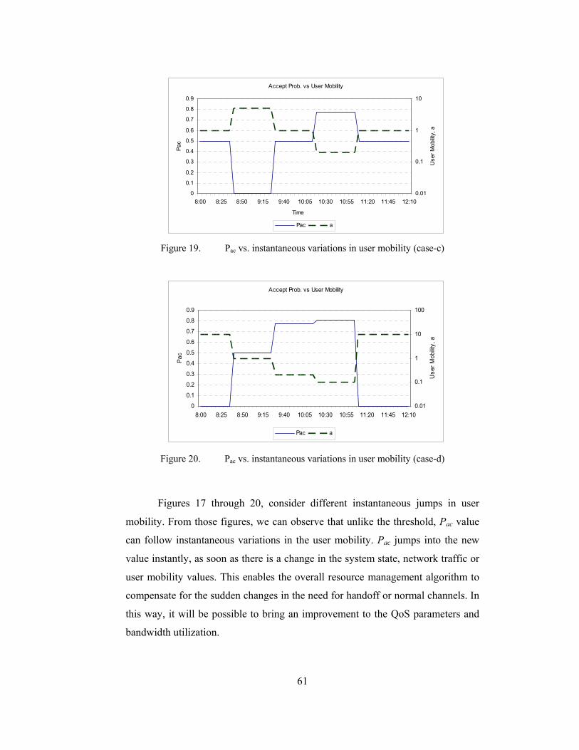
61

Figure 19. Pac vs. instantaneous variations in user mobility (case-c)

Figure 20. Pac vs. instantaneous variations in user mobility (case-d)

Figures 17 through 20, consider different instantaneous jumps in user

mobility. From those figures, we can observe that unlike the threshold, Pac value

can follow instantaneous variations in the user mobility. Pac jumps into the new

value instantly, as soon as there is a change in the system state, network traffic or

user mobility values. This enables the overall resource management algorithm to

compensate for the sudden changes in the need for handoff or normal channels. In

this way, it will be possible to bring an improvement to the QoS parameters and

bandwidth utilization.

Accept Prob. vs User Mobility

0

0.1

0.2

0.3

0.4

0.5

0.6

0.7

0.8

0.9

8:00 8:25 8:50 9:15 9:40 10:05 10:30 10:55 11:20 11:45 12:10

Pac

0.01

0.1

1

10

User

Mobility

, a

Pac a

Time

(min)

Accept Prob. vs User Mobility

0

0.1

0.2

0.3

0.4

0.5

0.6

0.7

0.8

0.9

8:00 8:25 8:50 9:15 9:40 10:05 10:30 10:55 11:20 11:45 12:10

Pa

c

0.01

0.1

1

10

100

Us

er

Mo

bili

ty,

aPac a

62

The purpose of the Pac is to bring a probabilistic approach to the new call

admission process, with the aim of increasing bandwidth utilization by preventing

unnecessary new call blockings. Dynamic channel reservation methods studied

from literature that reserve some radio channels for handoff calls, block out all

new call attempts once the regular channels are full, irrespective of the relative

magnitudes of handoff call arrivals and new call arrivals. This can result in poor

resource utilization and low Pb performance, especially in such cases where the

system state is above the threshold, that is, normal channels are all occupied and

the new call arrival rate is high compared to handoff call arrival rate. In those

cases, the reserved channels will remain empty due to low handoff call arrivals,

whereas new call attempts are refused due to lack of free normal channels. In the

following figures of Pac performance, without loss of generality, the cell capacity

is assumed 100 radio channels, and the threshold is assumed to be 50 radio

channels.

Figure 21. Pac vs. system state in DCR and DCRM

Figure 21 shows the Pac value with respect to system state for DCR and

DRCM methods, under different user mobility conditions. The DCR methods

considered are generic dynamic channel reservation methods studied from

literature that reserve some radio channels for handoff calls, under five different

user mobility values, starting from low mobility (a=0.1) till high mobility (a=5).

New Call Accept Probability

0

0.2

0.4

0.6

0.8

1

1.2

0 10 20 30 40 50 60 70 80 90 100

System State (i)

Pac

DCR Pac (a=0,1) Pac (a=0,5)

Pac (a=1) Pac (a=2) Pac (a=5)

Threshold

63

The x-axis is the value and the y-axis is the system state, that is, the number of

occupied channels. As seen on this figure, in DCR, once the system state is above

the threshold, independent of the user mobility and network traffic conditions,

new call attempts are totally blocked out (Pac = 0). This aims, of course, to

increase handoff success. However, it will result in unnecessary new call

blockings, which leads to very poor bandwidth utilization. Poor spectral efficiency

will occur especially in such cases where the system state is above the threshold

and the user mobility is very low.

In the proposed DRCM approach, once the system state is above the

threshold, new call attempts are not totally blocked and get access to the reserved

channels, as much as the new call accept probability allows. Unlike DCR, form

Figure 22 we see that new call accept probability values are different with respect

to the system state for five different user mobility cases, starting from low

mobility (a=0.1) to high mobility (a=5). The accept probability drops with

increasing system state. For high user mobility, meaning there are more handoff

calls than new calls, Pac drops faster with increasing system state, to give higher

chance to handoff calls. On the contrary, for low user mobility, meaning there are

more new call attempts than handoff call attempts, Pac drops slower with

increasing system state, to give higher chance to new calls. In this way, the

resource management algorithm tries to prevent unnecessary new call blockings,

which results in very poor bandwidth utilization.

In the case considered in Figure 22, the user mobility is low, meaning

there are more new calls than handoff calls, the new call accept probability does

not drop at a high rate, enabling more new call attempts to get access to reserved

channels. That is, if there are more new calls compared to handoff calls, new calls

are accepted with a higher probability. This will enable to utilize reserved radio

channels that would be normally remain empty due to low handoff arrival rate,

and prevent unnecessary blocking of new calls.

In the case considered in Figure 23, the user mobility is high, meaning there

are more handoff calls compared to new calls, the new call accept probability falls

64

down very fast, enabling the relatively higher handoff call arrivals to get access to

reserved channels.

Figure 22. Pac vs. system state in DRCM method under low user mobility

Figure 23. Pac vs. system state in DRCM method under high user mobility

5.1.3. User Mobility

An efficient resource management algorithm must control the amount of

reserved radio channels and the admission of new calls, depending on the relative

magnitudes of λh and λn, that is depending on the subscriber mobility of the

DRCM New Call Accept Probability

0

0.2

0.4

0.6

0.8

1

1.2

0 10 20 30 40 50 60 70 80 90 100

System State (i)

Pac

Pac (a = 0,1)

Threshold

Accept Region

Reject

Region

DRCM New Call Accept Probability

0

0.2

0.4

0.6

0.8

1

1.2

0 10 20 30 40 50 60 70 80 90 100

System State (i)

Pa

c

Pac (a = 5)

Threshold

Reject RegionAccept Region

65

region. Therefore, user mobility is the most important parameter of both the

threshold adjustment process and the new call admission process. These two

processes, in turn, form the main part of the overall resource management

algorithm. Therefore, the user mobility definition has a major effect on both the

reserved number of channels and new call acceptance.

As detailed in section 3.1, the “subscriber profile prediction algorithm”

makes use of call statistics of each individual mobile to derive the handoff

reservation requests. With a high probability, handoff reservation requests will

turn into real handoff calls in near future. This valuable information about the near

future’s expected mobility figures is included in the user mobility definition of

this study. We consider that it is important to include the handoff reservation

request in the definition of user mobility. In this way, the channel reservation

process and the new call admission process become ready for the near future

changes in the network traffic and user mobility, instead of following the changes.

In this study, the user behavior α is defined as the ratio of the weighted sum

of “handoff call arrival rate, λh” and “handoff reservation request arrival rate,

λhrq” to the “new call arrival rate, λn”, as given in the equation (5) in section 3.2.

The instantaneous value of α as defined in the equation (5) is used in the new call

admission process. However, for the resource reservation process, we use the

long-term average, as given in the equation (6).

The efficiency of both the resource reservation process and new call

admission process depends very much on the efficiency of how close the user

mobility definition can follow the actual subscriber mobility pattern of the area.

The success of the user mobility definition itself depends on two parameter sets.

The first set is the set of β parameters of equation (6), which are the weighting

parameters of the moving average of “measured” mobility of subscribers from

previous time intervals. The second set is the set of γ parameters of equation (5),

which are the relative weights of λh and λhrq, where we propose to derive the λhrq

from individual subscriber profile information.

We evaluate the performance of the user mobility definition in terms of how

well it can follow the actual mobility pattern of the environment, under different

66

operational field data, and compare the performance with the classical user

mobility definition. To study the effect of β and γ parameters on user mobility

performance, we have evaluated the performance of user mobility under:

i) Different distribution for the β parameters, like linear distribution,

exponential distribution,

ii) Different number of previous values of α and Nwin to be included

in the moving average, like Nwin =5, Nwin =10. The number of previous values of

α be included in the moving average are determined by Nwin in equation (6).

iii) Different relative weights of γ parameters, starting from γ1=0.1,

γ2=0.9, until γ1=0.9, γ2=0.1, with 0.1 steps,

iv) Different input data set of subscriber mobility, like field data

collected from the downtown area in the capital city from one of the GSM service

providers, field data from an area with higher mobility of subscribers, and field

data from four different regions with typical mobility characteristics (business

area, highway area, entertainment area, shopping area).

In those figures, the x-axis shows the time of the day. For better readability,

we have divided the 24-hour period into six parts, each covering a 4-hour period

with 5-minute time intervals. The vertical bars represent the observed field

mobility of subscriber. These are the actual subscriber mobility pattern of the area.

The triangular-line represent the classical user mobility found in the literature that

we have examined so far, and the square-line represents the modified user

mobility definition of this study that includes the handoff reservation requests

coming from the individual mobile call statistics.

The set of figures in Figure 24-38, are the results of a case where the

environment is a business area with the data set of subscriber mobility,

accordingly. Each figure covers a 4-hour period. The β parameters are

“exponentially distributed”, with 10 βi values in the moving average (Nwin =10).

The actual analysis considers each time a different relative value for the γ1 and γ2

are considered, starting from γ1=0.1, γ2=0.9, until γ1=0.9, γ2=0.1, with 0.1 steps.

However, in the below figures a subset of the γ1 and γ2 are presented, which are

67

(γ1=0.1, γ2=0.9), (γ1=0.5, γ2=0.5), and (γ1=0.9, γ2=0.1). Since in the period 00:00-

04:00 no major subscriber activities are observed, there is no major difference for

different values of γ1 and γ2, therefore this time period is excluded from the

figures.

68

Figure 24. User Mobility in business area with exponential distribution of β

parameters, and γ1=0.1, γ2=0.9

Figure 25. User Mobility in business area with exponential distribution of β

parameters, and γ1=0.5, γ2=0.5

Figure 26. User Mobility in business area with exponential distribution of β

parameters, and γ1=0.9, γ2=0.1

User Mobility, a

0.01

0.1

1

10

100

4:00 4:25 4:50 5:15 5:40 6:05 6:30 6:55 7:20 7:45

Time of Day

User M

obility

Field User Mobility

Calculated average mobility, classical appr.Calculated average mobility, modified appr.

User Mobility, a

0.01

0.1

1

10

100

4:00 4:25 4:50 5:15 5:40 6:05 6:30 6:55 7:20 7:45

Time of Day

User M

obility

Field User Mobility

Calculated average mobility, classical appr.Calculated average mobility, modif ied appr.

User Mobility, a

0.01

0.1

1

10

100

4:00 4:25 4:50 5:15 5:40 6:05 6:30 6:55 7:20 7:45

Time of Day

User

Mobility

Field User Mobility

Calculated average mobility, classical appr.Calculated average mobility, modified appr.

69

Figure 27. User Mobility in business area with exponential distribution of β

parameters, and γ1=0.1, γ2=0.9

Figure 28. User Mobility in business area with exponential distribution of β

parameters, and γ1=0.5, γ2=0.5

Figure 29. User Mobility in business area with exponential distribution of β

parameters, and γ1=0.9, γ2=0.1

User Mobility, a

0.01

0.1

1

10

100

8:00 8:25 8:50 9:15 9:40 10:05 10:30 10:55 11:20 11:45

Time of Day

User M

obility

Field User Mobility

Calculated average mobility, classical appr.Calculated average mobility, modif ied appr.

User Mobility, a

0.01

0.1

1

10

100

8:00 8:25 8:50 9:15 9:40 10:05 10:30 10:55 11:20 11:45

Time of Day

User M

obility

Field User Mobility

Calculated average mobility, classical appr.Calculated average mobility, modif ied appr.

User Mobility, a

0.01

0.1

1

10

100

8:00 8:25 8:50 9:15 9:40 10:05 10:30 10:55 11:20 11:45

Time of Day

User M

obility

Field User Mobility

Calculated average mobility, classical appr.Calculated average mobility, modif ied appr.

70

Figure 30. User Mobility in business area with exponential distribution of β

parameters, and γ1=0.1, γ2=0.9

Figure 31. User Mobility in business area with exponential distribution of β

parameters, and γ1=0.5, γ2=0.5

Figure 32. User Mobility in business area with exponential distribution of β

parameters, and γ1=0.9, γ2=0.1

User Mobility, a

0.01

0.1

1

10

100

12:00 12:25 12:50 13:15 13:40 14:05 14:30 14:55 15:20 15:45

Time of Day

User M

obility

Field User Mobility

Calculated average mobility, classical appr.Calculated average mobility, modified appr.

User Mobility, a

0.01

0.1

1

10

100

12:00 12:25 12:50 13:15 13:40 14:05 14:30 14:55 15:20 15:45

Time of Day

User M

obility

Field User Mobility

Calculated average mobility, classical appr.Calculated average mobility, modif ied appr.

User Mobility, a

0.01

0.1

1

10

100

12:00 12:25 12:50 13:15 13:40 14:05 14:30 14:55 15:20 15:45

Time of Day

User

Mobility

Field User Mobility

Calculated average mobility, classical appr.Calculated average mobility, modif ied appr.

71

Figure 33. User Mobility in business area with exponential distribution of β

parameters, and γ1=0.1, γ2=0.9

Figure 34. User Mobility in business area with exponential distribution of β

parameters, and γ1=0.5, γ2=0.5

Figure 35. User Mobility in business area with exponential distribution of β

parameters, and γ1=0.9, γ2=0.1

User Mobility, a

0.01

0.1

1

10

100

16:00 16:25 16:50 17:15 17:40 18:05 18:30 18:55 19:20 19:45

Time of Day

User M

obility

Field User Mobility

Calculated average mobility, classical appr.Calculated average mobility, modified appr.

User Mobility, a

0.01

0.1

1

10

100

16:00 16:25 16:50 17:15 17:40 18:05 18:30 18:55 19:20 19:45

Time of Day

User

Mobility

Field User Mobility

Calculated average mobility, classical appr.Calculated average mobility, modif ied appr.

User Mobility, a

0.01

0.1

1

10

100

16:00 16:25 16:50 17:15 17:40 18:05 18:30 18:55 19:20 19:45

Time of Day

User M

obility

Field User Mobility

Calculated average mobility, classical appr.Calculated average mobility, modif ied appr.

72

Figure 36. User Mobility in business area with exponential distribution of β

parameters, and γ1=0.1, γ2=0.9

Figure 37. User Mobility in business area with exponential distribution of β

parameters, and γ1=0.5, γ2=0.5

Figure 38. User Mobility in business area with exponential distribution of β

parameters, and γ1=0.9, γ2=0.1

User Mobility, a

0.01

0.1

1

10

100

20:00 20:25 20:50 21:15 21:40 22:05 22:30 22:55 23:20 23:45

Time of Day

User M

obility

Field User Mobility

Calculated average mobility, classical appr.Calculated average mobility, modif ied appr.

User Mobility, a

0.01

0.1

1

10

100

20:00 20:25 20:50 21:15 21:40 22:05 22:30 22:55 23:20 23:45

Time of Day

User M

obility

Field User Mobility

Calculated average mobility, classical appr.Calculated average mobility, modif ied appr.

User Mobility, a

0.01

0.1

1

10

100

20:00 20:25 20:50 21:15 21:40 22:05 22:30 22:55 23:20 23:45

Time of Day

User M

obility

Field User Mobility

Calculated average mobility, classical appr.Calculated average mobility, modif ied appr.

73

The set of figures presented in Figure 24-38, show that the modified user

mobility definition can follow the actual mobility of subscribers, better that the

classical approach. This is observed in all the periods, and for all the γ1 and γ2

values. The difference between the figures of same time period and different set of

γ1 and γ2 values, although being not very large, show that with increasing γ2

values, the effect of λhrq on user mobility definition with respect to λh is

increasing. As the effect of λhrq increases, the system can adapt better to the

subscriber mobility value of the next time interval. However, increasing γ2 too

much puts an overemphasis onto λhrq, and the user mobility starts to switch to the

next time interval subscriber mobility value, prematurely. Study on different

values of γ1 and γ2 parameters proved that γ1=0.5 and γ2=0.5, are suitable values.

Therefore, for the γ1 and γ2 parameters, we propose to use γ1=0.5 and γ2=0.5. We

believe that this is a fair and realistic definition for our purpose.

Table.1 User Mobility Parameters

Parameter Value

Scenario (Network traffic and

subscriber behavior)

Field data, business area, highway

area, entertainment area, shopping

area

Distribution of β parameters Exponential, linear

Weights of γ1 and γ2 parameters Starting from (γ1=0.1, γ2=0.9), until (γ1=0.9, γ2=0.1), with 0.1 steps

Window Size (Nwin) Different values like, Nwin=5, 10, 15

To analyze, in detail, the effects of different parameters on the performance

of the modified user mobility definition, wide range of values for the parameters

are considered during the performance analysis. The below table summarized all

cases and parameters considered.

Not to repeat many figures, we have presented just some sample results in

Figure 24-38. From the results of all the different cases considered, as well as

from Figure 24-38, we can deduce some important results. These are as follows:

74

i) With exponential distributed β parameters, as compared to linear

distribution, the modified user mobility definition can better follow the subscriber

mobility of the environment.

ii) As of γ parameters, with increasing γ2 values, the effect of λhrq on

user mobility definition, compared to λh, is increasing. As the effect of λhrq

increases, the system can adapt better to the subscriber mobility value of the next

time interval. However, increasing γ2 too much puts an overemphasis onto λhrq,

and the user mobility value starts to reflect the next time interval subscriber

mobility value, prematurely. We need to keep a balance between γ1 and γ2 values.

Therefore, for the γ1 and γ2 parameters, we propose to use γ1=0.5 and γ2=0.5. We

believe that this is a fair and realistic definition for our purpose.

iii) The modified user mobility definition could follow better the

subscriber mobility of the area, compared to the classical approach, under all

operational field input data sets.

iv) With Nwin=10, as compared to Nwin=5 case, the modified user

mobility definition could closer follow the subscriber mobility of the

environment. However, no noticeable difference has been observed for further

increasing Nwin.

From these observations, we can conclude that, for the user mobility using

exponentially distributed β parameters, and with γ1=0.5 and γ2=0.5 values, we can

reach a better user mobility definition, which is able to tack better the subscriber

mobility of the area.

5.1.4. Handoff call dropping probability

From a subscriber’s point of view, dropping a call, which is in progress, is

considered far more annoying than blocking a new call establishment attempt [6,

7, 8, 18]. Therefore, handoff call dropping probability, that is, the handoff failure

probability Pf is an important QoS parameter. An efficient resource management

algorithm must keep Pf within acceptable limits. We have analyzed the

performance of the NCR, FCR, DCR and DRCH approaches for the QoS

75

parameter Pf, using the separate mathematical system performance models, which

we derived for all those approaches in section 4.2.

We have used Microsoft Excel to formulate the mathematical system

performance models, and to make the numerical analysis. Once the mathematical

models are formulated, Microsoft Excel makes it very easy to consider many

scenarios and perform many numerical analyses. This is done by just copying the

originals model files and changing the network traffic and subscriber mobility

values related to the desired scenario.

Figures 55-57 show the results of the Pf performance analysis under various

user mobility conditions, and for a wide range of network traffic, starting from

very low load to very high load conditions.

Figure 39. Pf performance results for the high user mobility (α=2) case

Figure 39 shows the Pf performance results for the high user mobility (α=2)

case. From Figure 39, one can observe that channel reservation improves the Pf

performance. All the channel reservation techniques have improved Pf

performance, compared to the No Channel Reservation (NCR) case. For all

network traffic values, the NCR, which does not reserve any channels for handoff

calls and treats handoff call attempts and new call establishment attempts in the

same way, shows the poorest Pf performance. Even the simplest channels

reservation scheme FCR, which reserves a predefined fixed amount of radio

channels for handoff calls, shows a considerable improvement compared to the

Pf under High User Mobility

1.00E-12

1.00E-10

1.00E-08

1.00E-06

1.00E-04

1.00E-02

1.00E+00

2.00 4.00 6.00 8.00 10.00 12.00 14.00 16.00 18.00 20.00

Traffic Load

Pf

NCR FCR DCR DRCM

76

NCR case. However, since the case considered here assumes a relatively high user

mobility condition, the DCR, which adjusts its reserved channels dynamically

according to the local user mobility estimate within the cell of interest, reserves a

higher number of radio channels compared to the FCR case. Therefore, it has an

improved performance over the FCR case. The DRCM scheme shows improved

Pf performance, even when compared with DCR. This is thanks to the highly

adaptive threshold adjustment of DRCM. The DRCM scheme takes into account

not only the current user mobility figures from the operational environment, but

also the handoff reservation requests from the mobiles in the surrounding cells. In

this way, it becomes ready for the near future expected changes in the user

mobility conditions and reserves ideal number of channels for handoff calls.

Figure 40. Pf performance results for the normal user mobility (α=1) case

Figure 40 shows the Pf performance results for the normal user mobility

(α=1) case. In the normal user mobility case, the number of handoff call arrivals

and new call arrivals are the same. In this case, the number of reserved channels

for handoff calls is equal for all FCR, DCR and DRCM techniques. Therefore, Pf

performance is equal for all of them and better than the NCR technique.

Pf under Normal User Mobility

1.00E-12

1.00E-10

1.00E-08

1.00E-06

1.00E-04

1.00E-02

1.00E+00

2.00 4.00 6.00 8.00 10.00 12.00 14.00 16.00 18.00 20.00

Traff ic Load

Pf

NCR FCR DCR DRCM

77

Figure 41. Pf performance results for the low user mobility (α=0,5) case

Figure 41 shows the Pf performance results for the low user mobility

(α=0.5) case. From Figure 41, we can observe the effect of channel reservation on

Pf performance. For all network traffic values, all of the channel reservation

techniques perform far better than the NCR method. The FCR method performs

superior under this user mobility condition. This is due to overemphasized number

of reserved channels for handoff calls for this case. The drawback of this fact

shows up, as the poorest Pb performance. The DRCM proves good Pf

performance, without any drawback on Pb performance, as will be seen in the

following section.

5.1.5 New Call Blocking Probability

Reserving radio channels for handoff calls improves handoff-dropping

probability. This we have shown in section 5.1.4. Since we need to reserve radio

channels to improve handoff-dropping probability, some new call blocking

probability and BW utilization have to be sacrificed. However, reserving more

than necessary radio channels can end up with unnecessary new call blockings.

Unnecessary new call blockings results in poor radio channel utilization. From a

service provider’s point of view, however, the resource management algorithm

Pf under Low User M obility

1.00E-12

1.00E-10

1.00E-08

1.00E-06

1.00E-04

1.00E-02

1.00E+00

2.00 5.00 8.00 11.00 14.00 17.00 20.00

Traff ic Load

NCR FCR DCR DRCM

78

must utilize the radio channels in an efficient way to maximize revenue (valuation

is revenue per Kbps of spectrum).

In this section, we have analyzed the performance of the NCR, FCR, DCR

and DRCH approaches for the QoS parameter Pb, using the separate mathematical

system performance models, which we derived for all those approaches in section

4.2. Following figures summarize the results of the numerical analysis.

Figures 58-60 show the results of the Pb performance analysis under various

user mobility conditions, and for a wide range of network traffic from very low

load to very high load conditions.

Figure 42. Pb performance results for the high user mobility (α=2) case

Figure 42 shows the Pb performance results for the high user mobility (α=2)

case. Highest Pb performance is for the NCR scheme. This is, of course,

something expected. Since the NCR does not reserve any channels for the handoff

calls, least new call blocking will occur in the NCR case. Actually, for the NCR

the Pb and Pf figures are the same. Because NCR treats both handoff call attempts

and new call attempts equally, they have equal probability of being denied

service. The more reservations are made for handoff calls, the more new call

connections that are trying to access the resources will be denied. It is however

Pb under High User Mobility

1.00E-12

1.00E-10

1.00E-08

1.00E-06

1.00E-04

1.00E-02

1.00E+00

2.00 5.00 8.00 11.00 14.00 17.00 20.00

Traff ic Load

Pb

NCR FCR DCR DRCM

79

interesting to note that, although the DRCM scheme that reserves highest number

of channels for handoff calls in the high user mobility case, does not have poorest

Pb performance. We can observe a certain amount of improvement, compared to

the DCR case. We can observe that, although reserving higher number of channels

for the handoff calls under high user mobility conditions to improve Pf

performance, DRCM does not necessarily perform poorer than DCR in terms of

Pb. This simultaneous improvement in both Pb performance and Pf performance is

due to two facts. First, it is thanks to the simultaneous implementation of both the

channels reservation process and the new call admission process in the resource

management algorithm in DRCM, as explained in sections II.2 and II.3. Second, it

is thanks to the situation awareness of the near future’s expected subscriber

mobility value, which is coming from the call statistics kept by the individual

mobiles.

Figure 43. Pb performance results for the normal user mobility (α=1)

Figure 43 shows the Pb performance results for the unity user mobility (α=1)

case. In the “unity” user mobility case, the number of handoff call arrivals and

new call arrivals are the same. In this case, the number of reserved channels for

handoff calls is equal for all FCR, DCR and DRCM techniques. Normally, one

would expect same Pb performance for all of them, because the resource

reservation process of the DRCM method predicts same amount of radio channels

Pb under Normal User Mobilit y

1.00E-12

1.00E-10

1.00E-08

1.00E-06

1.00E-04

1.00E-02

1.00E+00

2.00 5.00 8.00 11.00 14.00 17.00 20.00

Traf f ic Load

NCR FCR DCR DRCM

80

for handoff calls as compared to FCR and DCR. Pb performance is, indeed equal

for FCR and DCR cases. However, the DRCM technique shows improved

performance, in the normal user mobility case as well. This is because; the new

call admission process prevents some unnecessary new call blockings.

Figure 44. Pb performance results for the low user mobility (α=0.5) case

Figure 44 shows the Pb performance results for the low user mobility

(α=0.5) case. From Figure 44 we can observe the poorest performance for the

FCR case, which for this user mobility value reserves more than necessary radio

channels for handoff calls. The DRCM technique, on the other hand, shows an

important improvement over the DCR case, even under low user mobility value.

5.2 Results of Software Simulations

We have performed several software simulation runs, to predict the Pf, Pb

and bandwidth utilization performances of the compared methods. These software

simulations were done both for 24-hour to simulate a whole day traffic, and for

one hour to simulate the peak-hour traffic. The scenarios considered and the

environments simulated include, but are not limited to, a network traffic range of

10%, 30%, 50%, 70%, and 90% of the total cell capacity, and a user mobility

range of low user mobility (α=0.5), unity user mobility (α=1), and high user

Pb under Low User M obility

1.00E-12

1.00E-10

1.00E-08

1.00E-06

1.00E-04

1.00E-02

1.00E+00

2.00 5.00 8.00 11.00 14.00 17.00 20.00

Traf f ic Load

NCR FCR DCR DRCM

81

mobility (α=2). We have chosen these values of network traffic and user mobility,

to match the scenarios and simulation environment to the cases considered in the

mathematical analysis part. The simulation run results of all the scenarios and

simulation environments considered are included in the CD provided. We present

the results of some typical runs here, in tabular form.

In the 24-hour simulation runs, both the user mobility and the network

traffic are time-varying. These follow actual network traffic and subscriber

mobility figures, as observed in collected field data. The user mobility values

given in the below analysis are the average of the 24-hour. The network traffic

values categorized as 10%, 30%, 50%, 70%, and 90% of the total cell capacity are

the peaks experience during the 24-hour.

Table-1 shows the simulation results of 24-hour simulation runs. The

scenarios considered have, on average, low network traffic (10% of the total cell

capacity). For the subscriber mobility, three separate user mobility characteristics

are considered. These are, low user mobility (α=0.5), unity user mobility (α=1),

and high user mobility (α=2).

From Table-2 we can observe that there are no blocked new calls or dropped

handoff calls, for all the user mobility values considered. This is something

expected, of course, since the scenario considered has low network traffic (10% of

the total cell capacity). For this low network traffic scenario, all the methods

under comparison behave similarly. These values prove the expected results of the

low user mobility case.

Table-3 shows other simulation results of 24-hour simulation run. In all the

three cases, the scenarios considered have moderate network traffic (50% of the

total cell capacity). For the subscriber mobility, again three separate user mobility

characteristics are considered. These are, low user mobility (α=0.5), unity user

mobility (α=1), and high user mobility (α=2).

82

Table-2 Results of the 24-hour simulation runs under low network traffic

(10% of the total cell capacity) conditions

Simulation Results

User Mobility NCR FCR DCR DRCM

Utilization 0.090 0.090 0.090 0.090

Pb 0.000 0.000 0.000 0.000 α α α α = 0.5

Pf 0.000 0.000 0.000 0.000

Utilization 0.100 0.100 0.100 0.100

Pb 0.000 0.000 0.000 0.000 α α α α = 1

Pf 0.000 0.000 0.000 0.000

Utilization 0.088 0.088 0.088 0.088

Pb 0.000 0.000 0.000 0.000 α α α α = 2

Pf 0.000 0.000 0.000 0.000

Table-3 Results of the 24-hour simulation runs under moderate network traffic

(50% of the total cell capacity) conditions

Simulation Results

User Mobility NCR FCR DCR DRCM

Utilization 0.425 0.376 0.408 0.418

Pb 0.036 0.204 0.104 0.070 α α α α = 0.5

Pf 0.039 0.000 0.003 0.016

Utilization 0.397 0.376 0.368 0.384

Pb 0.004 0.095 0.129 0.059 α α α α = 1

Pf 0.003 0.000 0.000 0.001

Utilization 0.393 0.379 0.360 0.376

Pb 0.000 0.075 0.195 0.103 α α α α = 2

Pf 0.001 0.000 0.000 0.000

From Table-3, we can observe that with that amount of traffic, there are

already some blocked new calls or dropped handoff calls, at least for some of the

methods compared and under some user mobility values considered. With this

network traffic amount, we can observe the effect of different resource

management algorithms implemented in the compared methods.

Table-4 shows, yet other 24-hour simulation run results. In all the three

cases, the scenarios considered have high network traffic (90% of the total cell

capacity). For the subscriber mobility, again three separate user mobility

characteristics are considered. These are, low user mobility (α=0.5), unity user

mobility (α=1), and high user mobility (α=2).

83

Table-4 Results of the 24-hour simulation runs under high network traffic

(90% of the total cell capacity) conditions

Simulation Results

User Mobility NCR FCR DCR DRCM

Utilization 0.662 0.554 0.632 0.652

Pb 0.210 0.488 0.307 0.258 α α α α = 0.5

Pf 0.244 0.001 0.098 0.156

Utilization 0.600 0.496 0.522 0.569

Pb 0.167 0.509 0.440 0.329 α α α α = 1

Pf 0.173 0.001 0.004 0.031

Utilization 0.600 0.517 0.488 0.531

Pb 0.164 0.600 0.700 0.551 α α α α = 2

Pf 0.157 0.019 0.016 0.021

Table-4 shows the simulation results for 24-hour simulation run, for an area

with high network traffic characteristics. Since the network traffic is very high, we

notice some important performance differences. The NCR method satisfies the

desired Pf performance (Pf,target=0.1) in non of the user mobility cases considered.

All the channels reservation methods bring improvement to the Pf performance.

However, since the network traffic considered is very high, the improvement in Pf

performance has a deep impact on Pb performance. In the FCR and DCR cases,

the adverse effect on Pb performance is very high, especially in the high mobility

case, as expected. This is the main reason of the drop in channel utilization, for

the FCR and DCR cases. Just like in the mathematical analysis part, the software

simulation under the given scenario predict that, the DRCM has improved channel

utilization and Pb performance compared to the FCR and DCR cases. The effect

of the two-way implementation in the resource management algorithm, which are

the resource reservation and new call admission processes, shows itself as

improved Pb performances and higher spectral efficiency in the DRCM case

compared to the FCR and DCR cases.

The scenario simulated in this case has high network traffic. Therefore, in

Table-4 we can observe relatively high blocked new calls or dropped handoff

calls. Although the case considered here is a high network traffic scenario, the

bandwidth utilization figures are, somehow low compared to what someone

84

would expect under that much network traffic. This is because, the simulation run

covers a 24-hour period, during which the peak network traffic reaches 90% of the

total cell capacity. The handoff call droppings and new call blockings are mainly

from such network traffic peaks. This leads us to the peak-hour simulations.

To have a better understanding about the peak hour behavior of the

compared methods, we have performed separate simulation runs for the peak-hour

analysis. Besides the Pf, Pb and bandwidth utilization results, in the peak-hour

simulation results we have also recorded the handoff and new call count, and the

handoff call drops and new call blockings, to have a better understanding about

call statistics. We have presented these in the below tables related to peak-hour

performance results.

In the peak-hour simulation runs, the mean values of the call arrivals are

constant over the simulation period. We have categorized the scenarios and

simulation environments in terms of network traffic and user mobility, according

to the mean values of the call arrivals.

The performance results of all network traffic and user mobility cases

evaluated are included in the attached CD. Since there are no major performance

differences for the low network traffic conditions, as it was in the 24-hour

simulation case, we provide here the performance results of high network traffic

scenarios with a number of different user mobility cases.

Table-5 Peak-Hour simulation results under high network traffic

and low user mobility (α=0.3) conditions

Peak Hour Simulation Results

NCR FCR DCR DRCM

Channel Utilization 0,904 0,765 0,792 0,857

Pb 0,138 0,290 0,287 0,176

Pf 0,129 0,000 0,000 0,024

New Call Count

(Blocked/Total) 330/2391 687/2367 688/2394 399/2271

Handoff Call Count

(Dropped/Total) 76 / 589 0 / 574 0 / 580 15 / 613

Table-5 shows the peak-hour simulation run results for high network traffic

(90% of the total cell capacity) and low user mobility (α=0.3) conditions. As in all

85

peak-hour simulation run results, in Table-10 we can see that the channel

utilizations are relatively high for all the methods under investigation, as

compared to the 24-hour simulation run results. This is because during the peak-

hour simulation runs, the radio network is heavily utilized continuously.

From Table-5, we can derive some important conclusion. Here again, the

NCR method, although having highest channel utilization, can not satisfies the

desired Pf performance (Pf,target=0.1). Since channel reservation methods need to

reserve some radio channels for handoff calls to improve handoff-dropping

probability, they have to sacrifice some new call blocking probability and BW

utilization. That is exactly what we observe in the FCR, DCR and DRCM

methods. All channel reservation methods bring improvement to the Pf

performance. However, this improvement is at a cost of increase in Pb

performance and decrease in channel utilization. Since the case considered in

Table-5 is a low user mobility case, meaning higher number of new calls

compared to handoff calls, reserving radio channels generously, combined with

high traffic figures, can bring considerable amount of adverse effect on Pb

performance. This is exactly what happens in the FCR and DCR cases. To prevent

76 handoff call droppings observed in the NCR case during one hour, both

methods cause over 350 additional new call blockings. The DRCM method, on

the other hand, prevents 65 handoff call droppings out of the 76, by just

sacrificing 69 additional new call attempts. This is, of course, a reasonable trade-

off, and the high spectral efficiency of the DRCM case verifies this trade-off.

Going through Tables 6-8, we can make similar observations and similar

conclusions. For example, in the equal handoff and new call arrival case, whose

results we present in Table-6, 321 handoff call drops occurred in the NCR case.

Both the FCR and DCR methods reduce this amount of handoff call drops to eight

handoff call drops, at a cost of more that 600 additional new call blockings. For

the DRCM method, this cost is 400 new calls only.

From Table-8, we can see that with the increasing user mobility, the FCR

and DCR methods are justified in their approach, to some extend. That is why the

bandwidth utilization of both methods is increasing with increasing user mobility.

86

With increasing mobility, the number of unnecessary new call blockings, that can

be detected and prevented by the DRCM method, becomes smaller and smaller.

Table-6 Peak-Hour simulation results under high network traffic

and low user mobility (α=0.5) conditions

Peak Hour Simulation Results

NCR FCR DCR DRCM

Channel Utilization 0.881 0.756 0.756 0.834

Pb 0.110 0.299 0.299 0.221

Pf 0.110 0.000 0.000 0.013

New Call Count

(Blocked/Total) 198 / 1793 526 / 1759 526 / 1759 397 / 1800

Handoff Call Count

(Dropped/Total) 133 / 1212 0 / 1202 0 / 1202 16 / 1220

Table-7 Peak-Hour simulation results under high network traffic

and unity user mobility (α=1) conditions

Peak Hour Simulation Results

NCR FCR DCR DRCM

Channel Utilization 0.915 0.799 0.798 0.862

Pb 0.177 0.509 0.507 0.395

Pf 0.178 0.005 0.004 0.037

New Call Count

(Blocked/Total) 313 / 1765 933 / 1834 932 / 1836 713 / 1808

Handoff Call Count

(Dropped/Total) 321 / 1801 8 / 1774 8 / 1776 68 / 1843

Table-8 Peak-Hour simulation results under high network traffic

and high user mobility (α=2) conditions

Peak Hour Simulation Results

NCR FCR DCR DRCM

Channel Utilization 0.908 0.805 0.796 0.819

Pb 0.162 0.526 0.609 0.482

Pf 0.176 0.011 0.002 0.021

New Call Count

(Blocked/Total) 192 / 1185 677 / 1288 771 / 1266 578 / 1198

Handoff Call Count

(Dropped/Total) 431 / 2454 26 / 2290 5 / 2370 49 / 2362

The aim of the software simulation runs was to prove the numerical

performance analysis, and to predict direct bandwidth utilization analysis. Careful

examination of the simulation results show that, the simulation runs predict indeed

similar performance results compared to the mathematical analysis results

87

obtained in section 5.1 about QoS parameters. We have performed a detailed

comparison of mathematical and simulation analysis results in section 5.3

In any software simulation, before reporting any results, we must prove that,

the results obtained are not due to random noise and are statistically significant.

Since the radio spectrum is a limited resource, the performance improvement of

any solution will not be huge compared to existing solutions. Therefore, in our

case, it is more important to prove that the performance improvement of the

proposed DRCM method predicted by the simulations is significant. One efficient

way to decide on the significance of the simulation results is to repeat the

simulations for the same scenario, without changing the environmental conditions,

until we can decide which results are real and which are random.

The simulation results presented in Table2 through Table8 consider a wide

range of network traffic and subscriber mobility. The simulation results proved to

be consistent with the mathematical results. However, these results were the

average obtained from three simulation runs for each case. Three simulations may

not be sufficient to decide on the stability and quality of the results. Therefore, we

need to perform a number of successive simulation runs to verify that the results

obtained are not due to random noise and the predicted performance differences

are statistically significant.

In any simulation, repeating simulation runs and changing nothing other

than the random number seeds can cause what appear to be large differences in

output. If we are to use simulation in real problems, we need a means how to tell

which effects are random and which are real. In the GPSS World, the “Analysis of

Variance (ANOVA)” command provides a way for this purpose. The ANOVA

command makes a first level of statistical analysis relatively easy. After one has

fully tested a simulation under a variety of conditions, one will probably want the

answers to some questions from the simulation. That is where experimentation

comes in. In order to predict the effects of factors under our control, we will need

to simulate each of the possibilities and determine if the result exceeds that due

only to random variation. The ANOVA command in GPSS provides an efficient

way for this purpose.

88

Keeping in mind that little number of runs for a specific scenario may not be

enough to decide that the results are statistically significant; we have performed

many runs or "replicas" for each of four methods compared, and for every

scenario considered. Replicas are runs of identical conditions except that a

different set of seeds is used to prime the pseudo-random number generators. This

provides a baseline of variability due only to random effects. It will show us

whether the results obtained are statistically significant, and are not due to random

noise only.

When we use statistical methods to see if two alternatives are different in

performance, we must not allow extraneous uncontrolled events to occur during

the simulations. It would not be fair to load one run with additional activities at

some unknown place in the simulation, and not to do precisely the same thing in

all other runs. Therefore, we have used the same seed set that belongs to a specific

scenario for all the methods compared. Since our results are in the form of an

arithmetic average of many results, we are justified in using the ANOVA

command to do a statistical analysis. Using the ANOVA block statement, we have

derived the statistical mean and variance of the performance parameters Pb, Pf

and bandwidth utilization, from the successive simulation runs, for each case

under consideration.

For each scenario and environmental conditions considered, and for each of

the four methods compared, we have performed successive simulation runs, and

recorded the results from the ANOVA output file. Figure 45 illustrates a sample

ANOVA output file. From this file, we can read the mean and variance of the QoS

parameter under investigation. As a starting point, we started with 10 replications

for each scenario and environmental conditions considered, and repeated these 10

replications for all the four methods compared.

89

Anova (Pbresults, 2, 2) ANOVA Source of Sum of Degrees of Mean Square F Critical Value Variance Squares Freedom of F (p=.05) A 0.000 0 Error 0.087 44 0.002 Total 0.087 44 Treatment Level Count Mean Min Max 95% C.I. (SE) A 1 45 0.198 0.167 0.335 (0.185, 0.211) Variance 0.0443941 Anova (Pfresults, 2, 2) ANOVA Source of Sum of Degrees of Mean Square F Critical Value Variance Squares Freedom of F (p=.05) A 0.000 0 Error 0.066 44 0.002 Total 0.066 44 Treatment Level Count Mean Min Max 95% C.I. (SE) A 1 45 0.096 0.009 0.132 (0.084, 0.108) Variance 0.0387694 Anova (Unresults, 2, 2) ANOVA Source of Sum of Degrees of Mean Square F Critical Value Variance Squares Freedom of F (p=.05) A 0.000 0 Error 0.030 44 0.001 Total 0.030 44 Treatment Level Count Mean Min Max 95% C.I. (SE) A 1 45 0.895 0.799 0.923 (0.887, 0.902) Variance 0.0261210

Figure 45. Sample Analysis of Variance (ANOVA) output file

90

To see the effect of the replications on the performance, we have repeated

the replications, each time with increased number of simulation runs in each

replication. The increments were additional five repetitions at each stage. As we

can see from Figures 46-51, repeating replications beyond 50 simulation runs

turned to be useless, since we could observe no noticeable difference in

performance after 40-50 simulation runs.

Figure 46 through Figure 51 show the results of a scenario where the

network traffic is relatively high (90% of total cell capacity), and the user mobility

is low (α=0.5). In those figures, we present the mean and variance of Pb, Pf and

bandwidth utilization, as the output of successive runs. The x-axis shows the

number of successive simulation runs, which we have performed each time with a

different seed set. The purpose of running many successive simulations is to

verify that the results are not due to random noise and the performance differences

observed are statistically significant. To have a fair comparison, we use the same

seed sets for all the four methods compared. We started with 10 successive

simulation runs for each case, and continued until there is no more performance

difference among the replications.

Figure 46-51 show the mean and variance of Pb, of the compared four

methods. The scenario considered is high network traffic (90% of total cell

capacity) and low user mobility (α=0.5) scenario. The replications start with a

replication of 10 simulation runs and extend to a replication with 60 simulation

runs. From the results presented in Figure 46-47, we can observe that there is a

clear and steady separation between the Pb performance figures of the four

methods compared. Besides, there is no much difference between the 10

simulation run results and the 60 simulation run results. Moreover, the variance

analysis results, presented in Figure 47, show small variance values. Therefore,

we can conclude from Figure 46-47, that the Pb performance results obtained are

statistically significant, and the performance difference among the compared

methods is well above random noise.

91

Figure 46. Pb Mean Analysis under high network traffic (90% of total cell capacity)

and low user mobility (α=0.5).

Figure 47. Pb Variance Analysis under high network traffic (90% of total cell

capacity) and low user mobility (α=0.5).

Figure 48-49 show the mean and variance of Pf, of the compared four

methods. The scenario considered is high network traffic (90% of total cell

capacity) and low user mobility (α=0.5) scenario. Again, the replications start

with a replication of 10 simulation runs and extend to a replication with 60

simulation runs. From the results presented in Figure 48-49, we can observe that

there is no much difference between the 10 simulation run results and the 60

simulation run results, and the results prove to be consistent. Moreover, the

variance analysis results, presented in Figure 49, show very small variance values,

compared to the respective mean values. Therefore, we can conclude from Figure

48-49, that the Pf performance results obtained are statistically significant, and the

performance difference among the compared methods is well above random noise.

Pb Mean Analysis

0.000

0.100

0.200

0.300

0.400

0.500

10 20 30 40 50 60

Number Of Sim Runs

Pb M

ean

NCR FCR DCR DRCM

Pb Variance Analysis

0.0000

0.0500

0.1000

0.1500

0.2000

10 20 30 40 50 60Number Of Sim Runs

Pb V

ariance

NCR FCR DCR DRCM

92

Figure 50-51 show mean and variance analysis results of the bandwidth

utilization. From the results presented in Figure 50, we can observe that the low

channel utilization for the FCR method, under this scenario with high network

traffic and low user mobility values, is persistent. Besides, the performances of

the dynamic reservation methods are stable and approach to that of the baseline

method (the NCR method). The very low variance figures presented in Figure 51,

compared to the high mean values, clears any doubts about the performance

differences in bandwidth utilization results being well above random noise, and

therefore being statistically significant.

The Pb, Pf, and utilization mean and variance analysis results presented in

Figure 50-51 proves a clear performance difference among the compared

methods. The results obtained using many replications prove that the performance

difference observed are not due to random noise. We conclude that the

performance improvement of the DRCM is statistically significant, at least for the

low user mobility case.

In Figure 46-51, we have presented the mean and variance analysis results,

derived from the replication simulation runs for a scenario of high network traffic

(90% of total cell capacity) and low user mobility (α=0.5). In order to have a

throughout study, and include all scenarios considered in the 24-hour and peak

hour simulation runs, as well as all cases considered in the mathematical analysis

part, we have repeated the replication runs to do the mean and variance analysis,

for the unity user mobility (α=1) and high user mobility (α=2) cases as well.

Results of the mean and variance analysis of high network traffic (90% of total

cell capacity) and unity user mobility (α=1) are presented in Figure 52-57, and the

results of the mean and variance analysis of high network traffic (90% of total cell

capacity) and high user mobility (α=2) are presented in Figure 58-63.

93

Figure 48. Pf Mean Analysis under high network traffic (90% of total cell capacity)

and low user mobility (α=0.5).

Figure 49. Pf Variance Analysis under high network traffic (90% of total cell

capacity) and low user mobility (α=0.5).

Figure 50. Bandwidth Utilization Mean Analysis under high network traffic (90% of

total cell capacity) and low user mobility (α=0.5).

Pf Mean Analysis

0.000

0.050

0.100

0.150

0.200

0.250

0.300

10 20 30 40 50 60

Number Of Sim Runs

Pf

NCR FCR DCR DRCM

Pf Variance Analysis

0.0000

0.0200

0.0400

0.0600

0.0800

0.1000

10 20 30 40 50 60Number Of Sim Runs

Pf

Va

ria

nc

e

NCR FCR DCR DRCM

Bandwith Utilization Mean Analysis

0.600

0.700

0.800

0.900

1.000

10 20 30 40 50 60

Number Of Sim Runs

Ba

nd

with

Utiliza

tio

n M

ea

n

NCR FCR DCR DRCM

94

Figure 51. Bandwidth Utilization Variance Analysis under high network traffic

(90% of total cell capacity) and low user mobility (α=0.5).

Figure 52. Pb Mean Analysis under high network traffic (90% of total cell capacity)

and unity user mobility (α=1).

Figure 53. Pb Variance Analysis under high network traffic (90% of total cell

capacity) and unity user mobility (α=1).

Bandwidth Utilization Variance Analysis

0.0000

0.0500

0.1000

0.1500

0.2000

10 20 30 40 50 60Number of Sim Runs

BW

Uti

liza

tio

n V

ar

NCR FCR DCR DRCM

Pb Mean Analysis

0

0.1

0.2

0.3

0.4

0.5

0.6

0.7

10 20 30 40 50

Number Of Sim Runs

Pb

Me

an

NCR FCR DCR DRCM

Pb Variance Analysis

0

0.01

0.02

0.03

0.04

0.05

10 20 30 40 50

Number Of Sim Runs

Pb

Va

ria

nc

e

NCR FCR DCR DRCM

95

Figure 54. Pf Mean Analysis under high network traffic (90% of total cell capacity)

and unity user mobility (α=1).

Figure 55. Pf Variance Analysis under high network traffic (90% of total cell

capacity) and unity user mobility (α=1).

Figure 56. Bandwidth Utilization Mean Analysis under high network traffic (90% of

total cell capacity) and low user mobility (α=1).

Pf Mean Analysis

0

0.1

0.2

0.3

0.4

0.5

10 20 30 40 50

Number Of Sim RunsP

f

NCR FCR DCR DRCM

Pf Variance Analysis

0

0.01

0.02

0.03

0.04

0.05

10 20 30 40 50

Number Of Sim Runs

Pf

Va

ria

nc

e

NCR FCR DCR DRCM

Bandwith Utilization Mean Analysis

0.5

0.6

0.7

0.8

0.9

1

10 20 30 40 50

Number Of Sim Runs

Ba

nd

with

Utiliza

tio

n M

ea

n

NCR FCR DCR DRCM

96

Figure 57. Bandwidth Utilization Variance Analysis under high network traffic

(90% of total cell capacity) and low user mobility (α=1).

Figure 58. Pb Mean Analysis under high network traffic (90% of total cell capacity)

and high user mobility (α=2).

Figure 59. Pb Variance Analysis under high network traffic (90% of total cell

capacity) and high user mobility (α=2).

Bandwidth Utilization Variance Analysis

0

0.01

0.02

0.03

0.04

0.05

10 20 30 40 50

Number of Sim Runs

BW

Uti

liza

tio

n

Va

ria

nc

e

NCR FCR DCR DRCM

Pb Mean Analysis

0

0.1

0.2

0.3

0.4

0.5

0.6

0.7

10 20 30 40 50

Number Of Sim Runs

Pb

Me

an

NCR FCR DCR DRCM

Pb Variance Analysis

0

0.01

0.02

0.03

0.04

0.05

10 20 30 40 50

Number Of Sim Runs

Pb

Va

ria

nc

e

NCR FCR DCR DRCM

97

Figure 60. Pf Mean Analysis under high network traffic (90% of total cell capacity)

and high user mobility (α=2).

Figure 61. Pf Variance Analysis under high network traffic (90% of total cell

capacity) and high user mobility (α=2).

Figure 62. Bandwidth Utilization Mean Analysis under high network traffic (90% of

total cell capacity) and high user mobility (α=2).

Pf Mean Analysis

0

0.05

0.1

0.15

0.2

10 20 30 40 50

Number Of Sim Runs

Pf

NCR FCR DCR DRCM

Pf Variance Analysis

0

0.01

0.02

0.03

0.04

0.05

10 20 30 40 50

Number Of Sim Runs

Pf

Va

ria

nc

e

NCR FCR DCR DRCM

Bandwith Utilization Mean Analysis

0.5

0.6

0.7

0.8

0.9

1

10 20 30 40 50

Number Of Sim Runs

Ba

nd

with

Uti

liza

tio

n M

ea

n

NCR FCR DCR DRCM

98

Figure 63. Bandwidth Utilization Variance Analysis under high network traffic

(90% of total cell capacity) and high user mobility (α=2).

Going through Figure 46 to Figure 63, we can derive some important

conclusions. The purpose of the replication runs was to prove that the

performance results predicted by the software simulation runs are statistically

significant. Our aim was to repeat each simulation run, for a specific method

under consideration and under a specific scenario, without changing any

environmental parameter, as many times as it is necessary, until we could be sure

about the stability and quality of the results that we have obtained. We could

observe that there was no much difference between the results of the replication

run consisting of 10 repeated simulations and the results of the replication run

consisting of 50 repeated simulations. Besides, the performance difference among

the methods under evaluation was stable. Moreover, the variance analysis proved

very small variance compared to the corresponding mean values of Pb, Pf, and

bandwidth utilization. Therefore, we could conclude that the simulation results for

the Pb, Pf, and spectral efficiency analysis were statistically significant.

The mean and variance analysis derived from the replication simulation

runs, not only proved the quality and stability of the software simulations results,

but also verified the mathematical analysis results derived in the previous section.

Section 5.4 provides a comparison of the mathematical analysis results and the

software simulation results.

Bandwidth Utilization Variance Analysis

0

0.01

0.02

0.03

0.04

0.05

10 20 30 40 50

Number of Sim Runs

BW

Uti

liza

tio

n

Va

ria

nc

e

NCR FCR DCR DRCM

99

5.3 Software Simulations under fixed Pf

The results of software simulations presented in Section 5.2 were somehow

difficult to compare because there were difficulties in finding a satisfactory basis

for comparisons. Such a common basis could be to fix one of the parameters, such

as Pf. In making simulations, the approach adopted was to fix Pf and determine

performance of the four different approaches for this fixed Pf value. This has been

done by an iterative procedure where input traffic was adjusted in a step by step

manner until the targeted Pf value is obtained. It was a time consuming procedure

where five different user mobility cases and five target Pf values were considered,

resulting in a total of 25 different scenarios. This procedure was repeated for each

of the four different approaches. Input of the simulation program, i.e. input traffic

was changed in a trial and error manner until Pf value was within an acceptable

range.

During simulations, values of carried traffic (successfully completed handoff

and new calls), lost traffic (dropped handoff calls and blocked new calls),

successful handoff calls, admitted new calls, dropped handoff calls and blocked

new calls were evaluated. The obtained results are presented in the following.

Figure 64 shows the carried traffic for all of the user mobility values. The

carried traffic is defined as the sum of successfully completed handoff calls and

the new calls admitted during one hour simulation period. They show the carried

traffic for the four compared methods under five different user mobility

conditions (α = 4, α = 2, α = 1, α = 0.5, and α = 0.25), and for five different

handoff failure probability values of Pf = 0.05, Pf = 0.10, Pf = 0.15, Pf = 0.20, and

Pf = 0.25. From the results, we have observed that the supported traffic per hour

increases with increasing handoff failure probability for all the methods

compared. This can be observed in Figure 64, from the increasing number of

supported traffic with respect to increasing Pf value for a specific mobility value.

The DRCM approach shows a clear improvement in terms of total supported

number of calls for most of the cases considered. The only case where the FCR

has shown better performance was the low user mobility cases.

100

One of the significant ways of comparing performance is look at the offered

traffic values. It gives a good indication of efficiency of channel reservation

process. Figure 65 gives simulation results as the ratio of carried traffic over the

offered traffic. By definition, offered traffic is the sum of handoff call arrivals and

new call arrivals, and carried traffic is the sum of successfully completed handoff

calls and new calls admitted. Results of a total of 25 simulation runs were

presented. The simulation runs cover the five mobility values (α = 4, α = 2, α = 1,

α = 0.5, α = 0.25), and for each of them five different Pf values (Pf = 0.05, Pf =

0.10, Pf = 0.15, Pf = 0.20, Pf = 0.25). From Figure 65, one can observe that, under

high carried traffic for a wide range of user mobility and network traffic

conditions, the DRCM method results in a fairly stable carried traffic over offered

traffic ratio. This is an indication that the DRCM method can maintain a desired

Pf value without causing unnecessarily high new call blockings. From Figure 65,

one can also observe that, for user mobility equal to one, i.e. equal handoff and

new call arrivals, the performance of the FCR approaches that of the DCR. This is

something expected since for unity user mobility the DCR predicts the same

amount of reserved capacity as FCR.

Figure 65 also shows ratio of carried traffic over offered traffic for all the

mobility conditions. It can be observed that DRCM was able to show fairly stable

performance in terms of carried traffic over offered traffic compared to the other

channels reservation methods. Furthermore, one conclude that FCR which shows

higher number of supported calls under low user mobility conditions can actually

provide this at the cost of very high input traffic. This is because of the fact that

FCR overemphasizes the importance of the handoff calls, rejecting a very large

number of new calls.

Another comparison that is performed is based on the lost traffic. Figure 66

illustrates the lost traffic during the peak hour simulation for all the methods

compared. Each figure shows the performance of the methods under a different

user mobility value. The lost traffic is due to the dropped handoff calls and

blocked new calls. Figure 66 proves the fact that the FCR supports higher number

of calls for low user mobility values, however, this at a cost of high lost traffic.

101

The set of figures presented in Figure 67 show the performance comparison

of the methods under evaluation in terms of a new concept. The two measures, Pf

and Pb reflect two quantities which are not closely linked. Any comparison which

takes into account only one of these two parameters could be misleading. In order

to avoid this, weighted sum of successful handoff calls, successful new calls,

dropped handoff calls and blocked new calls was studied. The weighted sum was

calculated as:

W =a1 x NC success + a2 x HC success – b1 x NC fail – b2 x HC fail

where weights were real numbers. We can interpret such a weighted sum as a

measure of net revenue earned by an operator. Plus sign means earning and minus

sign means lost revenue. Then, an operator can choose these weights to maximize

its earnings. This is equivalent to using a1, a2, b1, and b2 as guidelines for the

policies to be followed during selection of channel reservation and new call

rejection policies.

During this study, the effect of various values of a1, a2, b1, and b2 parameters

have been analyzed. It could be observed that increasing the weights for the

handoff performance parameters was increasing the performance gap between the

NCR case and the channel reservation methods. On the other hand, increasing the

weights for the new call admission performance was increasing the performance

gap between FCR and the two dynamic channels reservation methods DCR and

DRCM.

Results of five different set a1, a2, b1 and b2 values are provided in the

attached CD. Due to lack of space, the results of one set are provided here. As a

typical example, Figure 67 shows the performance comparison of the four

methods under a1=1, a2=2, b1=0.1 and b2=0.2. From graphs it can be seen that the

proposed DRCM method shows a superior performance compared to the other

methods in all of the scenarios considered.

102

Figure 64. Total Carried Traffic with respect to increasing Pf

Total Carried Traff ic Per Hour α = 1

(Successful New and Handoff Calls)

DRCM

FCR/DCR

NCR

2100

2200

2300

2400

2500

2600

2700

0,05 0,1 0,15 0,2 0,25 Pf

Total Carried Traff ic Per Hour α = 2

(Successful New and Handoff Calls)

DRCM

DCR

FCR

NCR

2100

2200

2300

2400

2500

2600

2700

0,05 0,1 0,15 0,2 0,25 Pf

Total Carried Traff ic Per Hour α = 4

(Successful New and Handoff Calls)

DRCM

DCR

FCR

NCR

2100

2200

2300

2400

2500

2600

0,05 0,1 0,15 0,2 0,25 Pf

Total Carried Traff ic Per Hour α = 0,5

(Successful New and Handoff Calls)

DRCM

DCR

FCR

NCR

2100

2200

2300

2400

2500

2600

2700

0,05 0,1 0,15 0,2 0,25 Pf

Total Carried Traff ic Per Hour α = 0,25

(Successful New and Handoff Calls)

DRCM

DCR

FCR

NCR

2100

2200

2300

2400

2500

2600

2700

0,05 0,1 0,15 0,2 0,25 Pf

103

Figure 65. Ratio of Carried Traffic over Offered Traffic

Carried Traffic / Offered Traff ic for α = 1

DRCM

DCR/FCR

NCR

0

0,2

0,4

0,6

0,8

1

0,05 0,1 0,15 0,2 0,25Pf

Carried Traffic / Offered Traff ic for α = 2

DRCM

DCR

FCR

NCR

0

0,2

0,4

0,6

0,8

1

0,05 0,1 0,15 0,2 0,25 Pf

Carried Traff ic / Offered Traff ic for α = 4

DRCM

DCRFCR

NCR

0

0,2

0,4

0,6

0,8

1

0,05 0,1 0,15 0,2 0,25 Pf

Carried Traffic / Offered Traffic for α = 0,5

DRCM

DCR

FCR

NCR

0

0,2

0,4

0,6

0,8

1

0,05 0,1 0,15 0,2 0,25Pf

Carried Traff ic / Offered Traff ic for α = 0,25

DRCM

DCR

FCR

NCR

0

0,2

0,4

0,6

0,8

1

0,05 0,1 0,15 0,2 0,25 Pf

104

Figure 66. Lost Traffic

Lost Traff ic for α = 1

(Sum of Dropped Handoff Calls and

Blocked New Calls)

DRCM

DCR/ FCR

NCR

0

500

1000

1500

2000

2500

3000

3500

0,05 0,1 0,15 0,2 0,25Pf

Lost Traff ic for α = 2

(Sum of Dropped Handoff Call and Blocked

New Calls)

DRCM

DCR

FCR

NCR

0

500

1000

1500

2000

2500

3000

3500

0,05 0,1 0,15 0,2 0,25 Pf

Lost Traff ic for α = 4

(Sum of Dropped Handoff Call and Blocked

New Calls)

DRCM

DCR

FCR

NCR

0

500

1000

1500

2000

2500

3000

3500

0,05 0,1 0,15 0,2 0,25Pf

Lost Traff ic for α = 0,5

(Sum of Dropped Handoff Call and Blocked

New Calls)

DRCM

DCR

FCR

NCR0

1000

2000

3000

4000

5000

6000

0,05 0,1 0,15 0,2 0,25Pf

Lost Traff ic for α = 0,25

(Sum of Dropped Handoff Call and Blocked

New Calls)

DRCMDCR

FCR

NCR0

2000

4000

6000

8000

10000

12000

14000

0,05 0,1 0,15 0,2 0,25 Pf

105

Figure 67. Weighted Sum of All Calls

Weighted Sum of all Calls for M = 4

a1x NCS + a2x HCS - b1x NCL - b2x HCL

4500

4750

5000

5250

5500

0,05 0,1 0,15 0,2 0,25

Pf

NCR FCR DCR DRCM

Weighted Sum of all Calls for M = 2

a1x NCS + a2x HCS - b1x NCL - b2x HCL

4500

4750

5000

5250

5500

0,05 0,1 0,15 0,2 0,25

Pf

NCR FCR DCR DRCM

Weighted Sum of all Calls for M = 1

a1x NCS + a2x HCS - b1x NCL - b2x HCL

4200

4400

4600

4800

5000

5200

5400

0,05 0,1 0,15 0,2 0,25

Pf

NCR FCR DCR DRCM

Weighted Sum of all Calls for M = 0,5

a1x NCS + a2x HCS - b1x NCL - b2x HCL

4250

4500

4750

5000

5250

0,05 0,1 0,15 0,2 0,25

Pf

NCR FCR DCR DRCM

Weighted Sum of all Calls for M = 0,25

a1x NCS + a2x HCS - b1x NCL - b2x HCL

3750

4000

4250

4500

4750

5000

5250

0,05 0,1 0,15 0,2 0,25

Pf

NCR FCR DCR DRCM

106

5.4 Comparison of Results of Mathematical Analysis and Software

Simulations

In section 5.1, we have presented the results of the mathematical analysis for

the two QoS parameters, namely Pb and Pf. These were the numerically calculated

Pb and Pf values for the four methods compared, based on the system performance

models, which we have derived in section 4.2. In the mathematical analysis part,

for given user mobility values, we have derived Pb and Pf as a function of network

traffic, covering a full range of network traffic.

The aim of the software simulations, whose results we presented in section

5.2, was to verify the calculated theoretical results about the QoS parameters Pf

and Pb, and to provide direct spectral efficiency predictions. In the software

simulation part, we have simulated the resource management algorithms of the

four methods compared. The simulation programs, predict the Pb, Pf, and channel

utilization of the four methods compared, under given scenario and environmental

conditions. Software scenarios cover the network traffic and subscriber mobility

patters, environmental conditions cover parameters like the cell capacity.

To be able to perform fair and realistic comparisons about the numerical

results and simulation results, we need to base the comparisons on common

criteria in terms of network traffic and subscriber mobility. Under given

subscriber mobility figures, the numerical analysis presented in section 5.1 cover

a full range of network traffic, and the software simulation run on scenarios

describing network traffic and subscriber mobility.

The performance comparison figures below consist of two set of figures.

The first set consists of mathematical analysis results. These are the figures from

the section 5.1, redrawn however to detail the results of the high network traffic

load part. The second set of figures display the results of the software simulation

runs belonging to the high network load scenarios.

Going through figures 68-79, we can see that the performance parameters

predicted by the software simulations support to a large extend the values foreseen

by the theoretical calculations.

107

Figure 68. Pb results of mathematical analysis for low user mobility

Figure 69. Pb results of software analysis for low user mobility

Figure 70. Pf results of mathematical analysis for low user mobility

Pb under Low User Mobility

1.00E-03

1.00E-02

1.00E-01

1.00E+00

15.00 18.00 21.00

Traff ic Load

Pb

NCR FCR DCR DRCM

Pb under Low User Mobility

1.00E-03

1.00E-02

1.00E-01

1.00E+00

15.00 18.00 21.00

Traffic Load

Pb

NCR FCR DCR DRCM

Pf under Low User Mobility

1.00E-03

1.00E-02

1.00E-01

1.00E+00

15.00 18.00 21.00

Traffic Load

Pf

NCR FCR DCR DRCM

108

Figure 71. Pf results of software simulation for low user mobility

Figure 72. Pb results of mathematical analysis for unity user mobility

Figure 73. Pb results of software simulation for unity user mobility

Pf under Low User Mobility

1.00E-03

1.00E-02

1.00E-01

1.00E+00

15.00 18.00 21.00

Traffic Load

Pf

NCR FCR DCR DRCM

Pb under Normal User Mobility

1.00E-02

1.00E-01

1.00E+00

15.00 18.00 21.00

Traffic Load

Pb

NCR FCR DCR DRCM

Pb under Normal User Mobility

1.00E-02

1.00E-01

1.00E+00

15.00 18.00 21.00

Traffic Load

Pb

NCR FCR DCR DRCM

109

Figure 74. Pf results of mathematical analysis for unity user mobility

Figure 75. Pf results of software simulation for unity user mobility

Figure 76. Pb results of mathematical analysis for high user mobility

Pf under Normal User Mobility

1.00E-03

1.00E-02

1.00E-01

1.00E+00

15.00 18.00 21.00

Traffic Load

Pf

NCR FCR DCR DRCM

Pb under High User Mobility

1.00E-02

1.00E-01

1.00E+00

15.00 18.00 21.00

Traffic Load

Pb

NCR FCR DCR DRCM

Pf under Normal User Mobility

1,00E-03

1,00E-02

1,00E-01

1,00E+00

15,00 18,00 21,00

Traff ic Load

Pf

NCR FCR DCR DRCM

110

Figure 77. Pb results of software simulation for high user mobility

Figure 78. Pf results of mathematical analysis for high user mobility

Figure 79. Pf results of software simulation for high user mobility

5.5 Cost Analysis

The motivation of this study was the simultaneous satisfaction of three

main goals. These are;

i. Minimization of handoff calls droppings.

Pb under High User Mobility

1.00E-02

1.00E-01

1.00E+00

15.00 18.00 21.00

Traffic Load

Pb

NCR FCR DCR DRCM

Pf under High User Mobility

1.00E-03

1.00E-02

1.00E-01

1.00E+00

15.00 18.00 21.00

Traffic Load

Pf

NCR FCR DCR DRCM

Pf under High User Mobility

1.00E-03

1.00E-02

1.00E-01

1.00E+00

15.00 18.00 21.00

Traffic Load

Pf

NCR FCR DCR DRCM

111

ii. Minimization of new call blockings.

iii. Maximization of radio channels utilization.

From the subscriber’s point of view, it is important to minimize handoff

call droppings, and to minimize new call blockings. From the service provider’s

point of view, on the other hand, it is important to maintain a guaranteed level of

QoS for customer satisfaction, while at the same time to maximize the resource

utilization in order to maximize revenue.

Careful examination of the results obtained from the mathematical

analysis, as well as the software simulations, show that there is actually a trade-off

between dropping probabilities and blocking probabilities, and between dropping

probabilities and bandwidth utilization. Since we need to reserve some radio

channels to improve Pf, we have to sacrifice some new call blockings and

bandwidth utilization. It will be important to balance the trade-off between the

performance parameter. Therefore, a cost function has been defined to balance the

trade-off and to have a better understanding about the performances of the

compared methods. The cost function definition includes the three critical

parameters, BW, Pf, Pb and it is normalized with the baseline method, namely the

NCR case. Following a similar approach as in [1], the definition of the cost

function is as follows:

C = α (Pf,i / Pf,o) + β (Uo / Ui) + γ (Pb,i / Pb,o)

In this cost function definition, Uo, Pf,o, and Pb,o are the values of

bandwidth utilization, handoff call dropping probability, and new call dropping

probability of the baseline (NCR) case, respectively. The Ui, Pf,i, and Pb,i are the

values of bandwidth utilization, handoff call dropping probability, and new call

dropping probability of the method under comparison (one of FCR, DCR or

DRCM) case, respectively. α, β, and γ are the weights of handoff call dropping

probability, bandwidth utilization, and new call dropping probability, respectively.

The weights of the three parameters α, β, and γ are adjusted so that the cost

of the baseline case is C =1. Since an efficient resource management algorithm

must result in minimum cost for a wide range of relative weights of the three

112

parameters, we have compared the cost of the methods under consideration for

wide range feasible weights of U, Pf, and Pb.

The figures related to the cost analyses results are presented in Appendix-

D. As seen from all these figures, the cost function of the baseline case (NCR) is

equal to “one”, for all the relative weights of α, β, and γ. In each of these figures,

one of α, β, and γ weights are fixed, and the cost function variation is shown with

respect to variation in the other two parameters. Since the sum of the α, β, and γ

are equal to “one”, increase in one of the parameters means, of course, decrease in

the other. The figure in Appendix-D.1, shows the cost functions of the under fixed

BW weight (β=0,3), and increasing Pf weight (decreasing Pb weight). Here we can

observe two important facts;

i. All the channel reservation methods improve Pf performance. This can

be observed from the decreasing cost value with increasing Pf weight, for all the

compared methods.

ii. The proposed DRCM method can maintain a cost below the baseline

case for a wide range of feasible Pf weights.

The figure in Appendix-D.2 shows the cost functions under fixed Pb

weight (γ=0,3) and increasing BW weight (decreasing Pf weight). Here we can see

that the improvement in Pf performance for all the dynamic channel reservation

methods observed is actually at a cost of poorer BW utilization. This can be

observed from the increasing cost with increasing BW weight. The cost paid for

improving the Pf performance is especially high for the FCR and DCR methods.

For BW weights above 0,3 the FCR and DCR methods results in higher cost

compared to the baseline case, which is an indication of poor BW utilization. The

proposed DRCM method, on the other hand, can maintain a cost below the

baseline case for a wide range of feasible BW weights. This is due to the fact that,

DRCM brings a considerable improvement to handoff performance by better

utilizing the radio channels. From the fixed Pf weight (α=0,3) figure (increasing

BW weight, decreasing Pb weight) in Appendix-D.3, it can be observed that, the

proposed method can maintain lowest cost among the compared methods for the

same desired Pf performance.

113

CHAPTER VI

CONCLUSION

In today’s highly competitive markets, service providers try to achieve

simultaneous satisfaction of a high level of QoS and a high level of resource

utilization in order to maximize their revenues. Therefore, the objective of this

study has been to develop an efficient resource management algorithm to improve

handoff call dropping probability in a cellular system without degrading the QoS,

which has been a challenging task. It was considered to be useful to obtain and

analyze traffic data collected by one of the national 1800 MHz GSM service

providers. Two sets of data has been obtained and analyzed. The first set consists

of data collected from cells all over Turkey on a 24-hour basis. The second set

consists of one-week data from a cluster of cells in business area in Ankara.

Careful analysis of the data showed that the time and location dependent network

traffic load and subscriber mobility figures behave as expected. However, handoff

failure rates were higher than our expectations. Handoff failure rates were

especially critical during some heavy traffic periods. It has been the conclusion

that as cell sizes reduce in future generation mobile networks, resource

management algorithms will face problems that are difficult to solve if handoff

failure rates have to be limited to low levels for high QoS.

In order to evaluate the performances of the methods discussed,

mathematical models for NCR, FCR, DCR and DRCM were developed. The

results obtained using these models showed that reserving some radio channels for

handoff calls explicitly, improves Pf performance. This could be easily observed

from the performance difference between the NCR method and the channel

reservation methods, FCR, DCR and DRCM.

Both the network traffic load and the mobility of subscribers are time

varying. The field data analyzed in this study showed wide range of network

traffic and instantaneous variations in subscriber mobility. Therefore, the amount

of radio channels to be reserved for handoff calls at any moment can not be fixed

114

and must change adaptively. That is why; the FCR method could not guarantee

the desired Pf performance for all network traffic and subscriber mobility values.

From the results of section 5.1, we could see that, depending on the network

traffic and subscriber mobility values, the FCR can cause poor Pf and Pb

performance. The FCR method showed poor Pf performance for subscriber

mobility values that demand more radio channels and poor Pb performance for

low subscriber mobility values that need less radio channels than the FCR

assumes.

Unlike FCR, the DCR method tries to adjust adaptively the radio channels

reserved for handoff calls. It decides on the number of radio channels to be

reserved for the handoff calls depending on the mobility figures in the cell area.

The obtained results indicate that, in general, DCR performs better in terms of Pf

and Pb compared to the FCR. However, depending on the network traffic and

subscriber mobility values, the FCR may to be superior compared to the DCR, in

one or the other QoS parameter. This is because with its fixed amount of reserved

channels, FCR may be improving one or the other parameter. The result is either

poor QoS or poor bandwidth utilization.

If the network operator can get apriori information on subscriber behavior

and its mobility beforehand, it can apply an appropriate resource management

policy based on this information. In this way, the resource management algorithm

can realistically make changes in advance, in the way the traffic is handled, rather

than adapting to conditions with a delay. The DRCM method proposes a way to

provide this information, based on call statistics kept by each mobile using its own

resources. The DRCM method makes use of apriori information about mobility

statistics to decide on the most suitable number of radio channels to be reserved,

and in the new call admission process.

The results of analysis in section 5.1 showed that the DRCM technique

brings improvement to the Pb performance. It performs better than the DCR,

especially for low user mobility conditions. The DRCM, in general, showed

improved Pf performance as well compared to DCR, though not as high as the

improvement in Pb performance. It is important to note that this improvement in

115

Pf is not at the cost of decreased Pb performance. It is due to efficient utilization of

the radio channels. In other words, simultaneous improvement in the QoS and

radio channel utilization. It was also concluded that DRCM could adapt better to

instantaneous changes in network traffic and subscriber mobility, resulting in

better Pb and Pf performances.

Software simulations were done to verify the numerical results obtained

during the studies. Simulation studies were carried out in two steps. First, the

simulations were performed over a 24-hour period, i.e. over a full day. Second,

daily one-hour simulations were performed to simulate peak-hour times, i.e. under

heavy traffic conditions. From the results of the software simulation runs

presented in section 5.1, it was observed that simulation results conform to the

results of analysis. Moreover, the bandwidth utilization figures obtained from

simulation runs showed that the bandwidth efficiencies were consistent with the

predicted performances of QoS parameters. This fact can be observed from the

figures in section 5.3.

In this study, an efficient and feasible approach for subscriber profile

prediction has been proposed where individual mobiles drive statistical

information from their daily activities. Then, cell transition probabilities could be

obtained and decisions of whether to make a handoff reservation or not could be

based for each mobile separately, which could lead to very realistic scenarios.

Unfortunately, such a detailed modeling and simulation was beyond the means of

this study. Instead, average values which were in agreement with field data were

used. This detailed study could be the subject of further studies in the simulation

of cellular networks.

In summary, Channel reservation improves handoff success performance but

at a cost of an increase in the new call blocking probability. In parallel to this, a

substantial decrease in the channel utilization can be observed. Poor channel

utilization will occur if too many channels are reserved for handoff and stayed

empty. It has been demonstrated that dynamic radio channel reservation helps to

overcome these disadvantages to some extend by adaptively changing the number

of reserved radio channels according to changes user mobility and network traffic

116

conditions. Similar performance increases has been obtained in the DCR and

DRCM approaches. However, it is the conclusion that DRCM approach has the

potential of leading to considerable improvement in the handoff failure

performance by using the apriori information about hand off reservations and

using a probabilistic approach to the new call admissions. The performances

observed in simulations as well as in calculations were better when compared with

published DCR approaches. This improvement in handoff failure probability is

the result of better utilization of the radio channels.

As a final step in studies, simulation results were repeated for fixed Pf

conditions to make better comparisons between performances of different

approaches. Furthermore, to create a suitable measure for comparing

performances of different methods as far as Pf and Pb are concerned, a weighted

sum of four important parameters were plotted versus traffic conditions. These

four parameters were number of successful handoff calls, dropped handoff calls,

new calls admitted and finally new calls rejected. This weighted average was a

good measure of net revenues earned by the operator since ongoing calls represent

earned revenue and rejected or dropped calls represent revenue lost under fixed Pf

conditions. The results have shown that, weighted average performance of the

proposed approach is satisfactory for most cases and it could be said that

improvement over investigated approaches were very clear.

117

APPENDIX A

Appendix-A.1 Operational Field Network Traffic Data

118

119

120

121

122

123

124

APPENDIX A

Appendix-A 2 Operational Field Handoff Traffic Data

125

126

127

128

129

130

131

APPENDIX A

Appendix-A.3 Cell-to-Cell Handoff Report

Target Source Attempts Failures % Fail % Data x y 14 2 14.29 79

x y 60 2 3.33 79

x y 202 13 6.44 79

x y 29 2 6.9 79

x y 55 6 10.91 79

x y 69 7 10.14 79

x y 44 3 6.82 79

x y 96 11 11.46 79

x y 32 4 12.5 79

x y 18 2 11.11 79

x y 98 6 6.12 79

x y 2 0 0 79

x y 1 0 0 79

x y 28 2 7.14 79

x y 0 0 0 79

x y 9 2 22.22 79

x y 179 11 6.15 79

x y 9 0 0 79

x y 29 4 13.79 79

x y 59 2 3.39 79

x y 88 5 5.68 79

x y 8 1 12.5 79

x y 7 0 0 79

x y 0 0 0 79

x y 187 11 5.88 79

x y 16 0 0 79

x y 275 12 4.36 79

x y 8 0 0 79

x y 50 1 2 79

x y 5 1 20 79

x y 32 2 6.25 79

x y 3 0 0 79

x y 28 0 0 79

x y 10 0 0 79

x y 32 1 3.12 79

x y 20 4 20 79

x y 31 4 12.9 79

x y 59 4 6.78 79

x y 23 0 0 79

x y 3 2 66.67 79

x y 7 0 0 79

x y 5 0 0 79

x y 12 0 0 79

132

APPENDIX A

Appendix-A 4 Cell Handover Type Report

CELL

ID

BSC

ID

MSC

ID

Daily Total

Number of

Successful

Intra Cell

Handovers

Daily Total

Number of

Failed Intra

Cell

Handovers

Daily Total

Number of

Intra cell

Handover

Attempts where

MS returns to

Old Channel

Daily Total

Number of

Successful

Inter Cell

Handovers

(Outgoing)

x y z 0 1 0 94

x y z 1 0 0 76

x y z 0 0 0 76

x y z 0 0 0 98

x y z 3 0 0 332

x y z 1 0 0 867

x y z 4 0 0 495

x y z 0 0 0 1848

x y z 9 1 0 1798

x y z 0 0 0 656

x y z 0 0 0 665

x y z 0 0 0 854

x y z 4 0 0 520

x y z 3 0 0 1345

x y z 6 1 0 1850

x y z 7 7 2 191

x y z 0 0 0 214

x y z 1 0 0 856

x y z 12 0 0 1193

x y z 0 1 0 397

x y z 52 4 0 1993

x y z 4 3 0 1378

x y z 15 0 0 1101

x y z 0 2 0 521

x y z 7 0 0 898

x y z 2 11 0 345

x y z 1 0 0 530

x y z 2 0 0 463

x y z 0 0 0 1048

x y z 1 0 0 821

x y z 0 0 0 574

x y z 1 0 0 1527

x y z 0 0 0 654

x y z 8 0 0 659

x y z 0 0 0 171

x y z 0 0 0 447

x y z 0 0 0 593

133

Appendix-A 4 Cell Handover Type Report (Continued)

Daily Total

Number of

Failed Inter-

Cell

Handovers

(Outgoing)

Daily Total

Number of

Inter-cell

Handover

Attempts where

MS returns to

Old Channel

Inter-Cell

Handover

Failure

Rate

%

Inter-Cell

Handover

Attempt Old

Channel

Return Rate

%

Daily Total

Number of

Successful

External

Handovers

Daily Total

Number of

Failed

External

Handovers

2 2 2.08 2.08 0 0

0 0 0.00 0.00 0 0

2 1 2.56 1.28 0 0

1 0 1.01 0.00 0 0

8 7 2.35 2.06 0 0

23 14 2.58 1.57 0 0

13 8 2.56 1.57 0 0

50 34 2.63 1.79 0 0

74 46 3.95 2.46 0 0

13 3 1.94 0.45 0 0

19 9 2.78 1.32 0 0

33 19 3.72 2.14 0 0

12 6 2.26 1.13 0 0

81 59 5.68 4.14 0 0

83 63 4.29 3.26 0 0

14 8 6.83 3.90 0 0

10 3 4.46 1.34 0 0

17 8 1.95 0.92 0 0

43 24 3.48 1.94 0 0

8 5 1.98 1.23 0 0

53 32 2.59 1.56 0 0

34 22 2.41 1.56 0 0

14 11 1.26 0.99 0 0

42 38 7.46 6.75 0 0

29 21 3.13 2.27 0 0

31 15 8.24 3.99 0 0

11 9 2.03 1.66 0 0

23 18 4.73 3.70 0 0

40 27 3.68 2.48 0 0

35 25 4.09 2.92 0 0

20 15 3.37 2.53 0 0

49 27 3.11 1.71 0 0

17 10 2.53 1.49 0 0

30 21 4.35 3.05 0 0

11 10 6.04 5.49 0 0

13 10 2.83 2.17 0 0

29 18 4.66 2.89 0 0

21 19 11.73 10.61 0 0

134

APPENDIX A

Appendix-A 5 Cell Handover Reason Report

CELL

ID

BSC

ID

MSC

ID

Number of

Handovers at

Bad Uplink

Quality

Number of

Handovers at

Bad

Downlink

Quality

Number of

Handovers to

better K-Cell

(Locating

Algorithm) due

to Downlink

Level

Number of

Handovers

due to

Exceeded

Time

Alignment

(Distance)

x y z 8 3 50 0

x y z 4 1 42 0

x y z 1 1 59 0

x y z 2 0 73 0

x y z 14 3 203 0

x y z 49 41 286 0

x y z 23 2 225 0

x y z 87 30 955 1

x y z 203 43 870 0

x y z 31 7 264 0

x y z 46 16 271 0

x y z 47 2 307 0

x y z 22 11 119 0

x y z 91 23 477 0

x y z 130 47 854 0

x y z 9 5 43 0

x y z 38 25 212 0

x y z 47 10 311 0

x y z 54 22 524 0

x y z 23 6 126 0

x y z 125 35 758 0

x y z 72 20 593 0

x y z 41 28 469 0

x y z 24 10 282 0

x y z 34 15 381 0

x y z 26 14 164 0

x y z 32 13 69 0

x y z 37 3 49 0

x y z 80 32 207 0

x y z 69 18 104 0

x y z 49 18 106 0

x y z 133 26 235 0

x y z 54 19 142 0

x y z 82 12 137 0

x y z 27 9 50 0

135

Appendix-A 5 Cell Handover Reason Report (Continued)

Number of

Handovers to better

L-Cell (Locating

Algorithm) due to

Power Budget

Handover

Attempts due

to Operation

and

Maintenance

Intervention

Handover Attempts

due to Cell Load

Sharing

(Other Reasons)

38 0 0

25 0 0

17 0 0

24 0 0

123 0 0

516 0 0

260 0 0

834 0 0

756 0 0

369 0 0

353 0 0

531 0 0

382 0 0

841 0 0

900 0 0

150 0 0

361 0 0

506 0 0

641 0 0

250 0 0

1131 0 0

734 0 0

580 0 0

244 0 0

500 0 0

228 0 0

429 0 0

399 0 0

768 0 0

667 0 0

421 0 0

1186 0 0

454 0 0

457 0 0

96 0 0

307 0 0

430 0 0

91 0 0

136

APPENDIX A

Appendix-A 6 Cell TCH Traffic Channel Report

CELL

ID

BSC

ID

MSC

ID

Cell

Busy

Hour

Cell Busy

Hour

Number of

Attempts

Cell Busy

Hour

Number of

Handover

Attempts

Cell Busy

Hour

Number of

Blocks

(Congestion

at

Assignment)

Cell Busy Hour

Successful MS

Channel

Establishment

on TCHs

x y z 19:00 86 10 0 84

x y z 18:00 119 4 2 117

x y z 12:00 38 10 0 35

x y z 11:00 50 17 0 48

x y z 20:00 258 29 0 257

x y z 20:00 274 87 0 265

x y z 22:00 228 30 0 227

x y z 19:00 685 148 0 680

x y z 19:00 1355 170 0 1312

x y z 19:00 358 56 0 357

x y z 19:00 343 80 0 338

x y z 19:00 402 51 0 402

x y z 22:00 131 27 0 130

x y z 15:00 791 96 0 778

x y z 19:00 908 130 0 901

x y z 13:00 88 24 0 84

x y z 22:00 124 18 0 124

x y z 20:00 272 64 0 268

x y z 20:00 532 57 0 528

x y z 21:00 151 25 0 150

x y z 19:00 1138 168 0 1126

x y z 16:00 662 105 0 653

x y z 14:00 479 96 0 475

x y z 13:00 174 31 0 173

x y z 19:00 513 109 0 511

x y z 22:00 93 31 0 91

x y z 10:00 244 47 0 238

x y z 14:00 296 50 0 294

x y z 13:00 545 84 0 537

x y z 21:00 532 127 0 481

x y z 17:00 336 46 0 334

x y z 18:00 573 101 0 556

x y z 13:00 158 52 0 152

x y z 20:00 253 83 0 247

x y z 13:00 122 8 0 121

x y z 14:00 158 32 0 156

x y z 20:00 238 72 0 235

x y z 19:00 207 21 0 202

x y z 22:00 133 46 0 125

137

Appendix-A 6 Cell TCH Traffic Channel Report (Continued)

Cell Busy

Hour

Successful

Handover

Establishment

on TCHs

Cell Busy Hour

TCH Dropped

Connections due

to RF-Losses

(TA, Low Signal

Strength, Bad

Quality, Suddenly

Lost

Connections)

Cell Busy

Hour TCH

Dropped

Connections

due to

Failures

Cell Busy

Hour

Traffic

(Erlangs)

Cell Busy

Hour

Number of

Dropped

TCH

Connections

per Erlang

Cell Busy

Hour

Mean

Holding

Time

(Seconds)

9 16 0 0.45 35.556 19.4

6 4 1 1.06 4.717 32.74

8 2 0 0.18 11.111 18.86

15 1 0 0.46 2.174 34.58

26 4 0 1.32 3.030 18.56

75 2 0 1.01 1.980 13.66

28 2 0 0.92 2.174 14.54

143 9 0 3.04 2.961 16.12

134 24 0 6.08 3.947 16.68

55 3 0 1.11 2.703 11.15

74 1 0 1.35 0.741 14.41

51 0 0 2.01 0.000 17.99

27 0 0 0.74 0.000 20.54

85 2 0 2.58 0.775 11.94

123 6 0 4.1 1.463 16.37

21 1 0 0.57 1.754 24.29

18 3 0 1.12 2.679 32.58

61 1 0 1.46 0.685 19.63

56 1 0 2.12 0.472 14.45

28 0 0 0.79 0.000 18.87

155 7 0 4.63 1.512 14.81

97 4 0 2.73 1.465 15.07

91 0 0 2.57 0.000 19.49

29 2 0 0.99 2.020 20.58

103 4 0 2.19 1.826 15.46

30 2 0 0.69 2.899 27.25

43 2 0 1.04 1.923 15.67

46 0 0 1.46 0.000 17.86

75 0 0 2.7 0.000 18.08

82 5 0 2.34 2.137 17.53

42 4 0 1.39 2.878 15

92 10 0 3.13 3.195 20.27

47 4 0 0.8 5.000 18.88

80 2 0 1.45 1.379 21.09

8 0 0 0.76 0.000 22.56

29 1 0 0.64 1.563 14.74

73 4 0 1.31 3.053 20.04

16 0 0 1.18 0.000 21.09

38 0 0 0.59 0.000 16.96

138

Appendix-A 6 Cell TCH Traffic Channel Report (Continued)

Cell

Busy

Hour

Number

of

Available

Channels

Cell

Busy

Hour

Blocked

Calls

%

Cell

Busy

Hour

Dropped

Calls

%

Cell Busy

Hour TCH

Assignment

Success

Rate %

Cell Daily

Total

Number

of

Attempts

Cell

Daily

Total

Number

of

Handover

Attempts

Cell Daily

Total

Number of

Blocks

(Congestion

at

Assignment)

13.8 0.00 21.33 97.67 846 156 31

12.5 1.68 4.50 98.32 1491 113 16

14 0.00 7.41 92.11 317 54 0

14 0.00 3.03 96.00 712 123 0

14 0.00 1.73 99.61 2740 309 0

14 0.00 1.05 96.72 3501 785 0

14 0.00 1.01 99.56 2574 481 0

14 0.00 1.68 99.27 8913 1649 0

22 0.00 2.04 96.83 16910 1955 0

14 0.00 0.99 99.72 3236 627 0

14 0.00 0.38 98.54 3060 626 0

14 0.00 0.00 100.00 5907 768 0

14 0.00 0.00 99.24 1820 421 0

14 0.00 0.29 98.36 8021 1259 0

14 0.00 0.77 99.23 12017 1710 0

14 0.00 1.59 95.45 1170 170 0

14 0.00 2.83 100.00 1266 178 0

14 0.00 0.48 98.53 3570 782 0

14 0.00 0.21 99.25 7006 1150 0

14 0.00 0.00 99.34 1981 372 0

14 0.00 0.72 98.95 13575 1942 12

14 0.00 0.72 98.64 8597 1373 0

14 0.00 0.00 99.16 6119 1001 0

14 0.00 1.39 99.43 2441 492 0

14 0.00 0.98 99.61 6195 826 0

14 0.00 3.28 97.85 1149 317 0

14 0.00 1.03 97.54 3591 522 0

14 0.00 0.00 99.32 3222 510 0

14 0.00 0.00 98.53 7066 949 0

14 0.00 1.25 90.41 4156 768 0

14 0.00 1.37 99.40 4528 538 0

14 0.00 2.16 97.03 8121 1412 0

14 0.00 3.81 96.20 2597 598 0

14 0.00 1.20 97.63 3131 689 0

14 0.00 0.00 99.18 1429 206 0

14 0.00 0.79 98.73 2185 387 0

14 0.00 2.47 98.74 2266 499 0

14 0.00 0.00 97.58 2126 159 0

14 0.00 0.00 93.98 1865 459 0

139

Appendix-A 6 Cell TCH Traffic Channel Report (Continued)

Cell Daily

Total TCH

Congestion

Time

Cell Daily

Total

Successful

MS Channel

Establish-

ment on

TCHs

Cell Daily

Total

Successful

Handover

Establish-

ment on

TCHs

Cell Daily Total

TCH Dropped

Connections due

to RF-Losses

(TA, Low Signal

Strength, Bad

Quality, Suddenly

Lost

Connections)

Cell Daily

Total TCH

Dropped

Connections

due to

Failures

Cell Daily

Total

Traffic

(Erlangs)

13 796 113 36 6 3.91

12 1446 76 35 13 8.19

0 308 48 5 0 1.35

0 701 112 6 0 3.97

0 2727 302 24 0 14.26

0 3403 696 29 0 11.11

0 2542 456 12 0 9.53

0 8756 1539 118 1 34.86

0 16410 1555 228 1 73.43

0 3190 581 13 0 12.51

0 3008 588 35 0 12.81

0 5864 755 19 1 24.18

0 1792 399 7 0 8.12

0 7950 1204 31 1 30

0 11914 1612 78 2 47.3

0 1146 157 15 0 4.99

0 1246 166 15 0 6.35

0 3531 762 16 0 14.62

0 6940 1091 50 0 25.86

0 1956 349 10 0 7.62

5 13426 1808 107 0 52.77

0 8504 1299 56 0 34.62

0 6055 955 43 0 26.1

0 2395 455 21 0 10.62

0 6091 755 38 0 25.64

0 1112 286 32 0 6.31

0 3540 486 20 0 12.67

0 3202 495 26 0 15.84

0 6982 882 45 1 30.9

0 4035 676 34 0 16.27

0 4476 491 25 0 15.55

0 7973 1281 73 0 39.65

0 2561 575 24 2 9.76

0 3062 627 26 0 12.22

0 1385 172 15 0 6.73

0 2150 360 16 0 7.05

0 2218 461 18 0 8.56

0 2090 130 32 0 10.01

0 1823 422 10 0 6.16

140

Appendix-A 6 Cell TCH Traffic Channel Report (Continued)

Cell Daily

Total

Number of

Dropped

TCH

Connections

per Erlang

Cell

Daily

Total

Mean

Holding

Time

(Sec)

Cell Daily

Total

Number of

Available

Channels

Cell Daily

Total

Number of

Defined

Channels

Cell Daily

Total

Blocked

Calls %

Cell Daily

Total

Dropped

Calls %

Cell Daily

Total TCH

Assign-

ment

Success

Rate

%

0.518 17.7 12.7 14 3.66 6.15 94.09

0.282 20.39 12.7 14 1.07 3.50 96.98

0.178 15.81 14 14 0.00 1.92 97.16

0.073 20.4 14 14 0.00 1.02 98.46

0.081 18.82 14 14 0.00 0.99 99.53

0.126 11.75 14 14 0.00 1.07 97.20

0.061 13.5 14 14 0.00 0.58 98.76

0.165 14.33 14 14 0.00 1.65 98.24

0.150 16.11 22 22 0.00 1.54 97.04

0.050 14.12 14 14 0.00 0.50 98.58

0.132 15.33 14 14 0.00 1.45 98.30

0.040 14.84 14 14 0.00 0.39 99.27

0.042 16.31 14 14 0.00 0.50 98.46

0.051 13.59 14 14 0.00 0.47 99.11

0.082 14.29 14 14 0.00 0.78 99.14

0.145 15.69 14 14 0.00 1.52 97.95

0.114 18.34 14 14 0.00 1.39 98.42

0.053 14.91 14 14 0.00 0.58 98.91

0.093 13.41 14 14 0.00 0.85 99.06

0.063 14.03 14 14 0.00 0.62 98.74

0.098 14.15 14 14 0.09 0.92 98.90

0.078 14.65 14 14 0.00 0.78 98.92

0.079 15.52 14 14 0.00 0.84 98.95

0.095 15.96 14 14 0.00 1.08 98.12

0.071 15.15 14 14 0.00 0.71 98.32

0.244 20.44 14 14 0.00 3.87 96.78

0.076 12.89 14 14 0.00 0.65 98.58

0.079 17.8 14 14 0.00 0.96 99.38

0.072 15.93 14 14 0.00 0.75 98.81

0.101 14.52 14 14 0.00 1.01 97.09

0.077 12.5 14 14 0.00 0.63 98.85

0.089 17.9 14 14 0.00 1.09 98.18

0.128 13.72 14 14 0.00 1.31 98.61

0.103 14.37 14 14 0.00 1.07 97.80

0.107 17.49 14 14 0.00 1.24 96.92

0.109 11.81 14 14 0.00 0.89 98.40

0.101 13.89 14 14 0.00 1.02 97.88

0.154 17.24 14 14 0.00 1.63 98.31

0.078 12.16 14 14 0.00 0.71 97.75

141

APPENDIX B

Appendix-B.1 NCR Source Code

; GPSS World Simulation Program, NCR Case

;*****************************************************************

; No Channel Reservation Model

;*****************************************************************

; Time Unit is one second

;*****************************************************************

; Initialization Part

;*****************************************************************

INITIAL X$NLossC,0 ;New Call Loss Count

INITIAL X$HLossC,0 ;Handoff Call Loss Count

INITIAL X$Ncount,0 ;New Call Arrival Count

INITIAL X$Hcount,0 ;Handoff Call Arrival Count

INITIAL X$Pb,0

;New call blocking probability

INITIAL x$Pf,0

;Handoff call dropping probability

INITIAL X$nn,1 ;Average new call arrival

INITIAL X$nh,1 ;Average handoff call arrival

INITIAL X$alpha,1 ;User Mobility

INITIAL X$Erl,0 ;Traffic Load

Alpha EQU nh/nn ;User Mobility

nsd EQU 60

;Average new call service duration

hsd EQU 40

;Average handoff call service duration

Cmax EQU 44 ;Number of channels

Thmax EQU Cmax ;Upper Limit for Threhold

Thmin EQU Cmax#(3/4) ;Lower Limit for Threhold

Thi EQU 44 ;Threshold

Channels STORAGE 44

;Storage Capacity is number of channels

Ch_Usage TABLE S$Channels,1,1,45

;Channel usage frequency

TPb TABLE X$Pb,0,0.05,20 ;Pb distribution

TPf TABLE X$Pf,0,0.05,20 ;Pf distribution

Talpha TABLE X$Alpha,0,0.1,30 ;Alpha distribution

TErl TABLE X$Erl,0,2,32

;Traffic Load distribution

;*****************************************************************

; Simulation Part

;*****************************************************************

Begh SAVEVALUE Hcount+,1

;Increment arrived handoff call

SAVEVALUE alpha,(X$nn/X$nh)

;User Mobility reverse ratio of interarrivals

SAVEVALUE

Erl,(((60/X$nn)/(60/nsd))+((60/X$nh)/(60/hsd)))

;Traffic Load - all in per min

GATE SNF Channels,Handloss ;Try for a line

ENTER Channels ;Connect call

ADVANCE (Exponential(1,0,hsd)) ;Speak for sd seconds

LEAVE Channels ;Free a Channel

TRANSFER ,TerminH

;Increase losscount only when channels are full

142

Handloss SAVEVALUE HLossC+,1

;Increment Handoff Losscount

TerminH SAVEVALUE Pf,(X$HLossC/X$Hcount)

;Calculate handoff call drop probability

TABULATE Ch_Usage

;Tabulate Channel Usage

TABULATE TPb

;Tabulate Pb

TABULATE TPf

;Tabulate Pf

TABULATE TErl

;Tabulate Erl

TABULATE Talpha

;Tabulate alpha

TRANSFER ,Fin

;Remove a transaction

;*****************************************************************

Begn SAVEVALUE Ncount+,1

;Increment arrived new call

SAVEVALUE alpha,(X$nn/X$nh)

;User Mobility reverse ratio of interarrivals

SAVEVALUEErl,(((60/X$nn)/(60/nsd))+((60/X$nh)/(60/hsd)))

;Traffic Load - all in per min

TEST LE S$Channels,Thi,Newloss

;Block new calls when Th is reached

GATE SNF Channels,Newloss

;Try for a line since threshold not reached

ENTER Channels

;Connect call

ADVANCE (Exponential(1,0,nsd))

;Speak for sd seconds

LEAVE Channels

;Free a Channel

TRANSFER ,TerminN

;Increase losscount only when channels are full

Newloss SAVEVALUE NLossC+,1

;Increment New call Losscount

TerminN SAVEVALUE Pb,(X$NLossC/X$Ncount)

;Calculate handoff call drop probability

TABULATE Ch_Usage

;Tabulate Channel Usage

TABULATE TPb

;Tabulate Pb

TABULATE TPf

;Tabulate Pf

TABULATE Talpha

;Tabulate alpha

TABULATE TErl

;Tabulate Erl

Fin TERMINATE

;Remove a transaction

;*****************************************************************

; Scenario and Traffic Generation Part

;*****************************************************************

; Call arrivals for 00:00-01:59

GENERATE (Exponential(1,0,2.5)),,,2880

;Handoff Call arrivals for one hour

SAVEVALUE nh,2.5

SAVEVALUE nn,5

143

TRANSFER ,Begh

GENERATE (Exponential(1,0,5)),,,1440

;New Calls arrivals for one hour

TRANSFER ,Begn

; Call arrivals for 02:00-03:59

GENERATE (Exponential(1,0,40)),,(2#3600),180

;Handoff Call arrivals for one hour

SAVEVALUE nh,40

SAVEVALUE nn,20

TRANSFER ,Begh

GENERATE (Exponential(1,0,20)),,(2#3600),360

;New Calls arrivals for one hour

TRANSFER ,Begn

; Call arrivals for 04:00-05:59

GENERATE (Exponential(1,0,80)),,(4#3600),90

;Handoff Call arrivals for one hour

SAVEVALUE nh,80

SAVEVALUE nn,40

TRANSFER ,Begh

GENERATE (Exponential(1,0,40)),,(4#3600),180

;New Calls arrivals for one hour

TRANSFER ,Begn

; Call arrivals for 06:00-07:59

GENERATE (Exponential(1,0,20)),,(6#3600),360

;Handoff Call arrivals for one hour

SAVEVALUE nh,20

SAVEVALUE nn,40

TRANSFER ,Begh

GENERATE (Exponential(1,0,40)),,(6#3600),180

;New Calls arrivals for one hour

TRANSFER ,Begn

; Call arrivals for 08:00-09:59

GENERATE (Exponential(1,0,2)),,(8#3600),3600

;Handoff Call arrivals for one hour

SAVEVALUE nh,2

SAVEVALUE nn,6

TRANSFER ,Begh

GENERATE (Exponential(1,0,6)),,(8#3600),1200

;New Calls arrivals for one hour

TRANSFER ,Begn

; Call arrivals for 10:00-11:59

GENERATE (Exponential(1,0,2)),,(10#3600),3600

;Handoff Call arrivals for one hour

SAVEVALUE nh,2

SAVEVALUE nn,2

TRANSFER ,Begh

GENERATE (Exponential(1,0,2)),,(10#3600),3600

;New Calls arrivals for one hour

TRANSFER ,Begn

; Call arrivals for 12:00-13:59

GENERATE (Exponential(1,0,1.25)),,(12#3600),5670

;Handoff Call arrivals for one hour

SAVEVALUE nh,1.25

SAVEVALUE nn,2.5

TRANSFER ,Begh

GENERATE (Exponential(1,0,2.5)),,(12#3600),2880

;New Calls arrivals for one hour

TRANSFER ,Begn

144

; Call arrivals for 14:00-15:59

GENERATE (Exponential(1,0,2)),,(14#3600),3600

;Handoff Call arrivals for one hour

SAVEVALUE nh,2

SAVEVALUE nn,2

TRANSFER ,Begh

GENERATE (Exponential(1,0,2)),,(14#3600),3600

;New Calls arrivals for one hour

TRANSFER ,Begn

; Call arrivals for 16:00-17:59

GENERATE (Exponential(1,0,1.25)),,(16#3600),5760

;Handoff Call arrivals for one hour

SAVEVALUE nh,1.25

SAVEVALUE nn,2.5

TRANSFER ,Begh

GENERATE (Exponential(1,0,2.5)),,(16#3600),2880

;New Calls arrivals for one hour

TRANSFER ,Begn

; Call arrivals for 18:00-19:59

GENERATE (Exponential(1,0,1)),,(18#3600),7200

;Handoff Call arrivals for one hour

SAVEVALUE nh,1

SAVEVALUE nn,4

TRANSFER ,Begh

GENERATE (Exponential(1,0,4)),,(18#3600),1800

;New Calls arrivals for one hour

TRANSFER ,Begn

; Call arrivals for 20:00-21:59

GENERATE (Exponential(1,0,2)),,(20#3600),3600

;Handoff Call arrivals for one hour

SAVEVALUE nh,2

SAVEVALUE nn,6

TRANSFER ,Begh

GENERATE (Exponential(1,0,6)),,(20#3600),1200

;New Calls arrivals for one hour

TRANSFER ,Begn

; Call arrivals for 22:00-23:59

GENERATE (Exponential(1,0,5)),,(22#3600),1440

;Handoff Call arrivals for one hour

SAVEVALUE nh,5

SAVEVALUE nn,10

TRANSFER ,Begh

GENERATE (Exponential(1,0,10)),,(22#3600),720

;New Calls arrivals for one hour

TRANSFER ,Begn

;*****************************************************************

; Timing Part

;*****************************************************************

GENERATE 3600

;Xact each hour (Sim Couter in Hours)

TERMINATE 1

;*****************************************************

; INCLUDE "seed45.txt"

; Include-file to run the successive simulations

;*****************************************************************

; End NCR

;*****************************************************************

145

Appendix-B.2 FCR Source Code

; GPSS World Simulation Program, FCR Case

;*****************************************************************

; Fixed Channel Reservation Model

;*****************************************************************

; Time Unit is one second

;*****************************************************************

; Initialization Part

;*****************************************************************

INITIAL X$NLossC,0 ;New Call Loss Count

INITIAL X$HLossC,0 ;Handoff Call Loss Count

INITIAL X$Ncount,0 ;New Call Arrival Count

INITIAL X$Hcount,0 ;Handoff Call Arrival Count

INITIAL X$alpha,1 ;User Mobility

INITIAL X$Erl,0 ;Traffic Load

INITIAL X$Pb,0 ;New call blocking probability

INITIAL X$Pf,0 ;Handoff call dropping probability

INITIAL X$nn,1 ;Average new call arrival

INITIAL X$nh,1 ;Average handoff call arrival

Alpha EQU nh/nn ;User Mobility

nsd EQU 60 ;Average new call service duration

hsd EQU 40 ;Average handoff call service duration

Cmax EQU 44 ;Number of channels

Thmax EQU Cmax ;Upper Limit for Threhold

Thmin EQU Cmax#(1/2);Lower Limit for Threhold

Thi EQU Cmax#(3/4) ;Threshold

Channels STORAGE 44

;Storage Capacity is number of channels

Ch_Usage TABLE S$Channels,1,1,45

;Channel usage frequency

TPb TABLE X$Pb,0,0.05,20 ;Pb distribution

TPf TABLE X$Pf,0,0.05,20 ;Pf distribution

Talpha TABLE X$Alpha,0,0.1,30 ;Alpha distribution

TErl TABLE X$Erl,0,2,32

;Traffic Load distribution

;*****************************************************************

; Simulation Part

;*****************************************************************

Begh SAVEVALUE Hcount+,1

;Increment arrived handoff call

Begh SAVEVALUE Hcount+,1

;Increment arrived handoff call

SAVEVALUE Alpha,(X$nn/X$nh)

;User Mobility reverse ratio of interarrivals

SAVEVALUE

Erl,(((60/X$nn)/(60/nsd))+((60/X$nh)/(60/hsd)))

;Traffic Load - all in per min

GATE SNF Channels,Handloss ;Try for a line

ENTER Channels ;Connect call

ADVANCE (Exponential(1,0,hsd)) ;Speak for sd seconds

LEAVE Channels ;Free a Channel

TRANSFER ,TerminH

;Increase losscount only when channels are full

Handloss SAVEVALUE HLossC+,1

;Increment Handoff Losscount

TerminH SAVEVALUE Pf,(X$HLossC/X$Hcount)

146

;Calculate handoff call drop probability

TABULATE Ch_Usage

;Tabulate Channel Usage

TABULATE TPb

;Tabulate Pb

TABULATE TPf

;Tabulate Pf

TABULATE Talpha

;Tabulate alpha

TABULATE TErl

;Tabulate Erl

TRANSFER ,Fin

;Remove a transaction

;*****************************************************************

Begn SAVEVALUE Ncount+,1

;Increment arrived new call

SAVEVALUE Alpha,(X$nn/X$nh)

;User Mobility reverse ratio of interarrivals

SAVEVALUE

Erl,(((60/X$nn)/(60/nsd))+((60/X$nh)/(60/hsd)))

;Traffic Load - all in per min

TEST LE S$Channels,Thi,Newloss

;Block new calls when Thi is reached

GATE SNF Channels,Newloss

;Try for a line since threshold not reached

ENTER Channels

;Connect call

ADVANCE (Exponential(1,0,nsd))

;Speak for sd seconds

LEAVE Channels

;Free a Channel

TRANSFER ,TerminN

;Increase losscount only when channels are full

Newloss SAVEVALUE NLossC+,1

;Increment New call Losscount

TerminN SAVEVALUE Pb,(X$NLossC/X$Ncount)

;Calculate handoff call drop probability

TABULATE Ch_Usage

;Tabulate Channel Usage

TABULATE TPb

;Tabulate Pb

TABULATE TPf

;Tabulate Pf

TABULATE Talpha

;Tabulate alpha

TABULATE TErl

;Tabulate Erl

Fin TERMINATE

;Remove a transaction

;*****************************************************************

; Scenario and Traffic Generation Part

;*****************************************************************

; Call arrivals for 00:00-01:59

GENERATE (Exponential(1,0,2.5)),,,2880

;Handoff Call arrivals for one hour

SAVEVALUE nh,2.5

SAVEVALUE nn,5

TRANSFER ,Begh

GENERATE (Exponential(1,0,5)),,,1440

147

;New Calls arrivals for one hour

TRANSFER ,Begn

; Call arrivals for 02:00-03:59

GENERATE (Exponential(1,0,40)),,(2#3600),180

;Handoff Call arrivals for one hour

SAVEVALUE nh,40

SAVEVALUE nn,20

TRANSFER ,Begh

GENERATE (Exponential(1,0,20)),,(2#3600),360

;New Calls arrivals for one hour

TRANSFER ,Begn

; Call arrivals for 04:00-05:59

GENERATE (Exponential(1,0,80)),,(4#3600),90

;Handoff Call arrivals for one hour

SAVEVALUE nh,80

SAVEVALUE nn,40

TRANSFER ,Begh

GENERATE (Exponential(1,0,40)),,(4#3600),180

;New Calls arrivals for one hour

TRANSFER ,Begn

; Call arrivals for 06:00-07:59

GENERATE (Exponential(1,0,20)),,(6#3600),360

;Handoff Call arrivals for one hour

SAVEVALUE nh,20

SAVEVALUE nn,40

TRANSFER ,Begh

GENERATE (Exponential(1,0,40)),,(6#3600),180

;New Calls arrivals for one hour

TRANSFER ,Begn

; Call arrivals for 08:00-09:59

GENERATE (Exponential(1,0,2)),,(8#3600),3600

;Handoff Call arrivals for one hour

SAVEVALUE nh,2

SAVEVALUE nn,6

TRANSFER ,Begh

GENERATE (Exponential(1,0,6)),,(8#3600),1200

;New Calls arrivals for one hour

TRANSFER ,Begn

; Call arrivals for 10:00-11:59

GENERATE (Exponential(1,0,2)),,(10#3600),3600

;Handoff Call arrivals for one hour

SAVEVALUE nh,2

SAVEVALUE nn,2

TRANSFER ,Begh

GENERATE (Exponential(1,0,2)),,(10#3600),3600

;New Calls arrivals for one hour

TRANSFER ,Begn

; Call arrivals for 12:00-13:59

GENERATE (Exponential(1,0,1.25)),,(12#3600),5670

;Handoff Call arrivals for one hour

SAVEVALUE nh,1.25

SAVEVALUE nn,2.5

TRANSFER ,Begh

GENERATE (Exponential(1,0,2.5)),,(12#3600),2880

;New Calls arrivals for one hour

TRANSFER ,Begn

; Call arrivals for 14:00-15:59

148

GENERATE (Exponential(1,0,2)),,(14#3600),3600

;Handoff Call arrivals for one hour

SAVEVALUE nh,2

SAVEVALUE nn,2

TRANSFER ,Begh

GENERATE (Exponential(1,0,2)),,(14#3600),3600

;New Calls arrivals for one hour

TRANSFER ,Begn

; Call arrivals for 16:00-17:59

GENERATE (Exponential(1,0,1.25)),,(16#3600),5760

;Handoff Call arrivals for one hour

SAVEVALUE nh,1.25

SAVEVALUE nn,2.5

TRANSFER ,Begh

GENERATE (Exponential(1,0,2.5)),,(16#3600),2880

;New Calls arrivals for one hour

TRANSFER ,Begn

; Call arrivals for 18:00-19:59

GENERATE (Exponential(1,0,1)),,(18#3600),7200

;Handoff Call arrivals for one hour

SAVEVALUE nh,1

SAVEVALUE nn,4

TRANSFER ,Begh

GENERATE (Exponential(1,0,4)),,(18#3600),1800

;New Calls arrivals for one hour

TRANSFER ,Begn

; Call arrivals for 20:00-21:59

GENERATE (Exponential(1,0,2)),,(20#3600),3600

;Handoff Call arrivals for one hour

SAVEVALUE nh,2

SAVEVALUE nn,6

TRANSFER ,Begh

GENERATE (Exponential(1,0,6)),,(20#3600),1200

;New Calls arrivals for one hour

TRANSFER ,Begn

; Call arrivals for 22:00-23:59

GENERATE (Exponential(1,0,5)),,(22#3600),1440

;Handoff Call arrivals for one hour

SAVEVALUE nh,5

SAVEVALUE nn,10

TRANSFER ,Begh

GENERATE (Exponential(1,0,10)),,(22#3600),720

;New Calls arrivals for one hour

TRANSFER ,Begn

;*****************************************************************

; Timing Part

;*****************************************************************

GENERATE 3600

;Xact each hour (Sim Couter in Hours)

TERMINATE 1

;*****************************************************************

; INCLUDE "seed45.txt"

; Include-file to run the successive simulations

;*****************************************************************

; End FCR

;*****************************************************************

149

Appendix-B.3 DCR Source Code

; GPSS World Simulation Program, DCR Case

;*****************************************************************

; Dynamic Channel Reservation Model

;*****************************************************************

; Time Unit is one second

;*****************************************************************

; Initialization Part

;*****************************************************************

INITIAL X$NLossC,0 ;New Call Loss Count

INITIAL X$HLossC,0 ;Handoff Call Loss Count

INITIAL X$Ncount,0 ;New Call Arrival Count

INITIAL X$Hcount,0 ;Handoff Call Arrival Count

INITIAL X$Pb,0 ;New call blocking probability

INITIAL X$Pf,0 ;Handoff call dropping probability

INITIAL X$Thi,35 ;Instantaneous Value on Th

INITIAL X$alpha,1 ;User Mobility

INITIAL X$nn,1 ;Average new call arrival rate

INITIAL X$nh,1 ;Average handoff call arrival rate

INITIAL X$Erl,0 ;Traffic Load

INITIAL X$Loga,0 ;Log of user mobility

*INITIAL X$Pfi,0 ;A temporary variable

*INITIAL X$Pac,0 ;Accept probability

*Check VARIABLE (RN1/1000);Check is a r.v. between 0 and 1

nsd EQU 60 ;Average new call service duration

hsd EQU 40 ;Average handoff service duration

Cmax EQU 44 ;Number of channels

Thmax EQU Cmax ;Upper Limit for Threhold

Thmin EQU Cmax#(1/2);Lower Limit for Threhold

Thi EQU Cmax#(3/4) ;Threshold

Channels STORAGE 44 ;Storage Capacity is number of channels

Ch_Usage TABLE S$Channels,1,1,45 ;Channel usage

distribution

Threshold TABLE X$Thi,1,1,45 ;Threshold distribution

Talpha TABLE X$alpha,0,0.1,30 ;Alpha distribution

TErl TABLE X$Erl,0,2,32 ;Traffic Load distribution

TPb TABLE X$Pb,0,0.05,20 ;Pb distribution

TPf TABLE X$Pf,0,0.05,20 ;Pf distribution

*Tcheck TABLE V$check,0,0.05,20 ;r.v.

*Taccept TABLE X$Pac,0,0.05,20 ;Accept Prob. distribution

;*****************************************************************

; Simulation Part

;*****************************************************************

Begh SAVEVALUE Hcount+,1

;Increment arrived handoff call

SAVEVALUE Alpha,(X$nn/X$nh)

;User Mobility reverse ratio of interarrivals

SAVEVALUE

Erl,(((60/X$nn)/(60/nsd))+((60/X$nh)/(60/hsd)))

;Traffic Load - all in per min

SAVEVALUE Loga,(LOG(X$alpha))

;Calculate Log of user mobility

SAVEVALUE Thi,(X$Thi-(((Cmax-

Thmin)/Cmax)#(0.001#X$Loga)))

;Update Threshold

TEST LE X$Thi,Thmin,Notlow

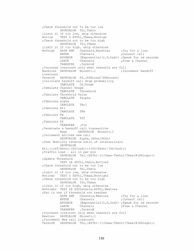
150

;Check threshold not to be too low

SAVEVALUE Thi,Thmin

;Limit it if too low, skip otherwise

Notlow TEST G X$Thi,Thmax,Nothigh

;Check threshold not to be too high

SAVEVALUE Thi,Thmax

;limit it if too high, skip otherwise

Nothigh GATE SNF Channels,Handloss ;Try for a line

ENTER Channels ;Connect call

ADVANCE (Exponential(1,0,hsd)) ;Speak for sd seconds

LEAVE Channels ;Free a Channel

TRANSFER ,TerminH

;Increase losscount only when channels are full

Handloss SAVEVALUE HLossC+,1 ;Increment Handoff

Losscount

TerminH SAVEVALUE Pf,(X$HLossC/X$Hcount)

;Calculate handoff call drop probability

TABULATE Ch_Usage

;Tabulate Channel Usage

TABULATE Threshold

;Tabulate Threshold Value

TABULATE Talpha

;Tabulate alpha

TABULATE TErl

;Tabulate Erl

TABULATE TPb

;Tabulate Pb

TABULATE TPf

;Tabulate Pf

TRANSFER ,Fin

;Terminate a handoff call transaction

Begn SAVEVALUE Ncount+,1

;Increment arrived new call

SAVEVALUE Alpha,(X$nn/X$nh)

;User Mobility reverse ratio of interarrivals

SAVEVALUE

Erl,(((60/X$nn)/(60/nsd))+((60/X$nh)/(60/hsd)))

;Traffic Load - all in per min

SAVEVALUE Thi,(X$Thi-(((Cmax-Thmin)/Cmax)#(X$Loga)))

;Update Threshold

TEST LE X$Thi,Thmin,Notlow2

;Check threshold not to be too low

SAVEVALUE Thi,Thmin

;Limit it if too low, skip otherwise

Notlow2 TEST G X$Thi,Thmax,Nothigh2

;Check threshold not to be too high

SAVEVALUE Thi,Thmax

;limit it if too high, skip otherwise

Nothigh2 TEST LE S$Channels,X$Thi,Newloss

;Pac is one if threshold not reached

GATE SNF Channels,Newloss ;Try for a line

ENTER Channels ;Connect call

ADVANCE (Exponential(1,0,nsd)) ;Speak for sd seconds

LEAVE Channels ;Free a Channel

TRANSFER ,TerminN

;Increase losscount only when channels are full

Newloss SAVEVALUE NLossC+,1

;Increment New call Losscount

TerminN SAVEVALUE Thi,(X$Thi-(((Cmax-Thmin)/Cmax)#(X$Loga)))

151

;Update Threshold

SAVEVALUE Pb,(X$NLossC/X$Ncount)

;Calculate handoff call drop probability

TABULATE Ch_Usage

;Tabulate Channel Usage

TABULATE Threshold

;Tabulate Threshold Value

TABULATE Talpha

;Tabulate alpha

TABULATE TErl

;Tabulate Erl

TABULATE TPb

;Tabulate Pb

TABULATE TPf

;Tabulate Pf

Fin TERMINATE

;Terminate a new call transaction

;*****************************************************************

; Scenario and Traffic Generation Part

;*****************************************************************

; Call arrivals for 00:00-01:59

GENERATE (Exponential(1,0,2.5)),,,2880

;Handoff Call arrivals for one hour

SAVEVALUE nh,2.5

SAVEVALUE nn,5

TRANSFER ,Begh

GENERATE (Exponential(1,0,5)),,,1440

;New Calls arrivals for one hour

TRANSFER ,Begn

; Call arrivals for 02:00-03:59

GENERATE (Exponential(1,0,40)),,(2#3600),180

;Handoff Call arrivals for one hour

SAVEVALUE nh,40

SAVEVALUE nn,20

TRANSFER ,Begh

GENERATE (Exponential(1,0,20)),,(2#3600),360

;New Calls arrivals for one hour

TRANSFER ,Begn

; Call arrivals for 04:00-05:59

GENERATE (Exponential(1,0,80)),,(4#3600),90

;Handoff Call arrivals for one hour

SAVEVALUE nh,80

SAVEVALUE nn,40

TRANSFER ,Begh

GENERATE (Exponential(1,0,40)),,(4#3600),180

;New Calls arrivals for one hour

TRANSFER ,Begn

; Call arrivals for 06:00-07:59

GENERATE (Exponential(1,0,20)),,(6#3600),360

;Handoff Call arrivals for one hour

SAVEVALUE nh,20

SAVEVALUE nn,40

TRANSFER ,Begh

GENERATE (Exponential(1,0,40)),,(6#3600),180

;New Calls arrivals for one hour

TRANSFER ,Begn

; Call arrivals for 08:00-09:59

152

GENERATE (Exponential(1,0,2)),,(8#3600),3600

;Handoff Call arrivals for one hour

SAVEVALUE nh,2

SAVEVALUE nn,6

TRANSFER ,Begh

GENERATE (Exponential(1,0,6)),,(8#3600),1200

;New Calls arrivals for one hour

TRANSFER ,Begn

; Call arrivals for 10:00-11:59

GENERATE (Exponential(1,0,2)),,(10#3600),3600

;Handoff Call arrivals for one hour

SAVEVALUE nh,2

SAVEVALUE nn,2

TRANSFER ,Begh

GENERATE (Exponential(1,0,2)),,(10#3600),3600

;New Calls arrivals for one hour

TRANSFER ,Begn

; Call arrivals for 12:00-13:59

GENERATE (Exponential(1,0,1.25)),,(12#3600),5670

;Handoff Call arrivals for one hour

SAVEVALUE nh,1.25

SAVEVALUE nn,2.5

TRANSFER ,Begh

GENERATE (Exponential(1,0,2.5)),,(12#3600),2880

;New Calls arrivals for one hour

TRANSFER ,Begn

; Call arrivals for 14:00-15:59

GENERATE (Exponential(1,0,2)),,(14#3600),3600

;Handoff Call arrivals for one hour

SAVEVALUE nh,2

SAVEVALUE nn,2

TRANSFER ,Begh

GENERATE (Exponential(1,0,2)),,(14#3600),3600

;New Calls arrivals for one hour

TRANSFER ,Begn

; Call arrivals for 16:00-17:59

GENERATE (Exponential(1,0,1.25)),,(16#3600),5760

;Handoff Call arrivals for one hour

SAVEVALUE nh,1.25

SAVEVALUE nn,2.5

TRANSFER ,Begh

GENERATE (Exponential(1,0,2.5)),,(16#3600),2880

;New Calls arrivals for one hour

TRANSFER ,Begn

; Call arrivals for 18:00-19:59

GENERATE (Exponential(1,0,1)),,(18#3600),7200

;Handoff Call arrivals for one hour

SAVEVALUE nh,1

SAVEVALUE nn,4

TRANSFER ,Begh

GENERATE (Exponential(1,0,4)),,(18#3600),1800

;New Calls arrivals for one hour

TRANSFER ,Begn

; Call arrivals for 20:00-21:59

GENERATE (Exponential(1,0,2)),,(20#3600),3600

;Handoff Call arrivals for one hour

SAVEVALUE nh,2

SAVEVALUE nn,6

TRANSFER ,Begh

153

GENERATE (Exponential(1,0,6)),,(20#3600),1200

;New Calls arrivals for one hour

TRANSFER ,Begn

; Call arrivals for 22:00-23:59

GENERATE (Exponential(1,0,5)),,(22#3600),1440

;Handoff Call arrivals for one hour

SAVEVALUE nh,5

SAVEVALUE nn,10

TRANSFER ,Begh

GENERATE (Exponential(1,0,10)),,(22#3600),720

;New Calls arrivals for one hour

TRANSFER ,Begn

;*****************************************************************

; Timing Part

;*****************************************************************

GENERATE 3600

;Xact each hour (Sim Couter in Hours)

TERMINATE 1

;*****************************************************

; INCLUDE "seed45.txt"

; Include-file to run the successive simulations

;*****************************************************************

; End DCR

;*****************************************************************

154

Appendix-B.4 DRCM Source Code

; GPSS World Simulation Program, DRCM Case

;*****************************************************************

; Dynamic Radio Channel Management Model

;*****************************************************************

; Time Unit is one second

;*****************************************************************

; Initialization Part

;*****************************************************************

INITIAL X$NLossC,0 ;New Call Loss Count

INITIAL X$HLossC,0 ;Handoff Call Loss Count

INITIAL X$Ncount,0 ;New Call Arrival Count

INITIAL X$Hcount,0 ;Handoff Call Arrival Count

INITIAL X$Pb,0 ;New call blocking probability

INITIAL X$Pf,0 ;Handoff call dropping probability

INITIAL X$Thi,35 ;Instantaneous Value on Th

INITIAL X$alpha,1 ;User Mobility

INITIAL X$nn,1 ;Average new call arrival rate

INITIAL X$nh,1 ;Average handoff call arrival rate

INITIAL X$Erl,0 ;Traffic Load

INITIAL X$Loga,0 ;Log of user mobility

INITIAL X$Pfi,0 ;A temporary variable

INITIAL X$Pac,0 ;Accept probability

Check VARIABLE (RN1/1000)

;Check is a r.v. between 0 and 1

nsd EQU 60 ;Average new call service duration

hsd EQU 40 ;Average handoff call service duration

Cmax EQU 44 ;Number of channels

Thmax EQU Cmax ;Upper Limit for Threhold

Thmin EQU Cmax#(1/2);Lower Limit for Threhold

Thi EQU Cmax#(3/4) ;Threshold

Channels STORAGE 44

;Storage Capacity is number of channels

Ch_Usage TABLE S$Channels,1,1,45

;Channel usage distribution

Threshold TABLE X$Thi,1,1,45

;Threshold distribution

Talpha TABLE X$Alpha,0,0.1,30

;Alpha distribution

TErl TABLE X$Erl,0,2,32

;Traffic Load distribution

Tcheck TABLE V$check,0,0.05,20 ;r.v.

Taccept TABLE X$Pac,0,0.05,20

;Accept Probability distribution

TPb TABLE X$Pb,0,0.05,20

;Pb Probability distribution

TPf TABLE X$Pf,0,0.05,20

;Pf Probability distribution

;*****************************************************************

; Simulation Part

;*****************************************************************

Begh SAVEVALUE Hcount+,1

;Increment arrived handoff call

SAVEVALUE alpha,(X$nn/X$nh)

;User Mobility reverse ratio of interarrivals

SAVEVALUE

Erl,(((60/X$nn)/(60/nsd))+((60/X$nh)/(60/hsd)))

155

;Traffic Load - all in per min

SAVEVALUE Loga,(LOG(X$alpha))

;Calculate Log of user mobility

SAVEVALUE Thi,(X$Thi-(((Cmax-Thmin)/Cmax)#(X$Loga)))

;Update Threshold

TEST LE X$Thi,Thmin,Notlow

;Check threshold not to be too low

SAVEVALUE Thi,Thmin

;Limit it if too low, skip otherwise

Notlow TEST G X$Thi,Thmax,Nothigh

;Check threshold not to be too high

SAVEVALUE Thi,Thmax

;limit it if too high, skip otherwise

Nothigh GATE SNF Channels,Handloss

;Try for a line

ENTER Channels ;Connect call

ADVANCE (Exponential(1,0,hsd))

;Speak for sd seconds

LEAVE Channels

;Free a Channel

TRANSFER ,TerminH

;Increase losscount only when channels are full

Handloss SAVEVALUE HLossC+,1

;Increment Handoff Losscount

TerminH SAVEVALUE Pf,(X$HLossC/X$Hcount)

;Calculate handoff call drop probability

TABULATE Ch_Usage

;Tabulate Channel Usage

TABULATE Threshold

;Tabulate Threshold Value

TABULATE Talpha

;Tabulate alpha

TABULATE TErl

;Tabulate Erl

TABULATE Tcheck

;Tabulate r.v. check

TABULATE Taccept

;Tabulate accept probability

TABULATE TPb

;Tabulate Pb probability

TABULATE TPf

;Tabulate Pf probability

Transfer ,Fin

;*****************************************************************

Begn SAVEVALUE Ncount+,1

;Increment arrived new call

SAVEVALUE alpha,(X$nn/X$nh)

;User Mobility reverse ratio of interarrivals

SAVEVALUE

Erl,(((60/X$nn)/(60/nsd))+((60/X$nh)/(60/hsd)))

;Traffic Load - all in per min

SAVEVALUE Thi,(X$Thi-(((Cmax-Thmin)/Cmax)#(X$Loga)))

;Update Threshold

TEST LE X$Thi,Thmin,Notlow2

;Check threshold not to be too low

SAVEVALUE Thi,Thmin

;Limit it if too low, skip otherwise

Notlow2 TEST G X$Thi,Thmax,Nothigh2

;Check threshold not to be too high

156

SAVEVALUE Thi,Thmax

;limit it if too high, skip otherwise

Nothigh2 SAVEVALUE Pac,(1)

;Pac is one if threshold not reached

TEST G S$Channels,X$Thi,Pacisok

;Pac is one if threshold not reached

SAVEVALUE Pfi,(SQR(COS((2#3.14#(S$Channels-

X$Thi))/(4#(Cmax-X$Thi)))))

;Calculate accept probability

SAVEVALUE Pac,((X$Alpha#((Cmax-S$Channels)/(Cmax-

X$Thi)))+((1-X$Alpha)#(X$Pfi)))

TEST L X$Pac,0,Pacisok

;don't let Pac become negative

SAVEVALUE Pac,(0)

;don't let Pac become negative

Pacisok TEST LE V$check,X$Pac,Newloss

;generate a r.n and check r.n with Pac

;accept the call if generated number is less than Pac

GATE SNF Channels,Newloss

;Try for a line

ENTER Channels

;Connect call

ADVANCE (Exponential(1,0,nsd))

;Speak for sd seconds

LEAVE Channels

;Free a Channel

TRANSFER ,TerminN

;Increase losscount only when channels are full

Newloss SAVEVALUE NLossC+,1

;Increment New call Losscount

TerminN SAVEVALUE Thi,(X$Thi-(((Cmax-

Thmin)/Cmax)#(0.001#X$Loga)))

;Update Threshold

SAVEVALUE Pb,(X$NLossC/X$Ncount)

;Calculate handoff call drop probability

TABULATE Ch_Usage

;Tabulate Channel Usage

TABULATE Threshold

;Tabulate Threshold Value

TABULATE Talpha

;Tabulate alpha

TABULATE TErl

;Tabulate Erl

TABULATE Tcheck

;Tabulate r.v. check

TABULATE Taccept

;Tabulate accept probability

TABULATE TPb

;Tabulate Pb probability

TABULATE TPf

;Tabulate Pf probability

Fin TERMINATE

;Terminate a new or handoff call transaction

;*****************************************************************

; Scenario and Traffic Generation Part

;*****************************************************************

; Call arrivals for 00:00-01:59

GENERATE (Exponential(1,0,2.5)),,,2880

;Handoff Call arrivals for one hour

157

SAVEVALUE nh,2.5

SAVEVALUE nn,5

TRANSFER ,Begh

GENERATE (Exponential(1,0,5)),,,1440

;New Calls arrivals for one hour

TRANSFER ,Begn

; Call arrivals for 02:00-03:59

GENERATE (Exponential(1,0,40)),,(2#3600),180

;Handoff Call arrivals for one hour

SAVEVALUE nh,40

SAVEVALUE nn,20

TRANSFER ,Begh

GENERATE (Exponential(1,0,20)),,(2#3600),360

;New Calls arrivals for one hour

TRANSFER ,Begn

; Call arrivals for 04:00-05:59

GENERATE (Exponential(1,0,80)),,(4#3600),90

;Handoff Call arrivals for one hour

SAVEVALUE nh,80

SAVEVALUE nn,40

TRANSFER ,Begh

GENERATE (Exponential(1,0,40)),,(4#3600),180

;New Calls arrivals for one hour

TRANSFER ,Begn

; Call arrivals for 06:00-07:59

GENERATE (Exponential(1,0,20)),,(6#3600),360

;Handoff Call arrivals for one hour

SAVEVALUE nh,20

SAVEVALUE nn,40

TRANSFER ,Begh

GENERATE (Exponential(1,0,40)),,(6#3600),180

;New Calls arrivals for one hour

TRANSFER ,Begn

; Call arrivals for 08:00-09:59

GENERATE (Exponential(1,0,2)),,(8#3600),3600

;Handoff Call arrivals for one hour

SAVEVALUE nh,2

SAVEVALUE nn,6

TRANSFER ,Begh

GENERATE (Exponential(1,0,6)),,(8#3600),1200

;New Calls arrivals for one hour

TRANSFER ,Begn

; Call arrivals for 10:00-11:59

GENERATE (Exponential(1,0,2)),,(10#3600),3600

;Handoff Call arrivals for one hour

SAVEVALUE nh,2

SAVEVALUE nn,2

TRANSFER ,Begh

GENERATE (Exponential(1,0,2)),,(10#3600),3600

;New Calls arrivals for one hour

TRANSFER ,Begn

; Call arrivals for 12:00-13:59

GENERATE (Exponential(1,0,1.25)),,(12#3600),5670

;Handoff Call arrivals for one hour

SAVEVALUE nh,1.25

SAVEVALUE nn,2.5

TRANSFER ,Begh

GENERATE (Exponential(1,0,2.5)),,(12#3600),2880

;New Calls arrivals for one hour

158

TRANSFER ,Begn

; Call arrivals for 14:00-15:59

GENERATE (Exponential(1,0,2)),,(14#3600),3600

;Handoff Call arrivals for one hour

SAVEVALUE nh,2

SAVEVALUE nn,2

TRANSFER ,Begh

GENERATE (Exponential(1,0,2)),,(14#3600),3600

;New Calls arrivals for one hour

TRANSFER ,Begn

; Call arrivals for 16:00-17:59

GENERATE (Exponential(1,0,1.25)),,(16#3600),5760

;Handoff Call arrivals for one hour

SAVEVALUE nh,1.25

SAVEVALUE nn,2.5

TRANSFER ,Begh

GENERATE (Exponential(1,0,2.5)),,(16#3600),2880

;New Calls arrivals for one hour

TRANSFER ,Begn

; Call arrivals for 18:00-19:59

GENERATE (Exponential(1,0,1)),,(18#3600),7200

;Handoff Call arrivals for one hour

SAVEVALUE nh,1

SAVEVALUE nn,4

TRANSFER ,Begh

GENERATE (Exponential(1,0,4)),,(18#3600),1800

;New Calls arrivals for one hour

TRANSFER ,Begn

; Call arrivals for 20:00-21:59

GENERATE (Exponential(1,0,2)),,(20#3600),3600

;Handoff Call arrivals for one hour

SAVEVALUE nh,2

SAVEVALUE nn,6

TRANSFER ,Begh

GENERATE (Exponential(1,0,6)),,(20#3600),1200

;New Calls arrivals for one hour

TRANSFER ,Begn

; Call arrivals for 22:00-23:59

GENERATE (Exponential(1,0,5)),,(22#3600),1440

;Handoff Call arrivals for one hour

SAVEVALUE nh,5

SAVEVALUE nn,10

TRANSFER ,Begh

GENERATE (Exponential(1,0,10)),,(22#3600),720

;New Calls arrivals for one hour

TRANSFER ,Begn

;*****************************************************

; Timing Part

;*****************************************************

GENERATE 3600

;Xact each hour (Sim Couter in Hours)

TERMINATE 1

;*****************************************************

; INCLUDE "seed45.txt"

; Include-file to run the successive simulations

;*****************************************************

; End DRCM

;*****************************************************

159

APPENDIX C

GPSS World Simulation Report - C4L4M05DRCM.342.1

Sunday, January 23, 2005 02:56:52

START TIME END TIME BLOCKS FACILITIES STORAGES

0.000 86400.000 131 0 1

NAME VALUE

ALPHA 10007.000

BEGH 1.000

BEGN 26.000

CHANNELS 10020.000

CHECK 10014.000

CH_USAGE 10021.000

CMAX 44.000

ERL 10010.000

FIN 57.000

HANDLOSS 15.000

HCOUNT 10003.000

HLOSSC 10001.000

HSD 40.000

LOGA 10011.000

NCOUNT 10002.000

NEWLOSS 46.000

NH 10009.000

NLOSSC 10000.000

NN 10008.000

NOTHIGH 10.000

NOTHIGH2 34.000

NOTLOW 8.000

NOTLOW2 32.000

NSD 60.000

PAC 10013.000

PACISOK 40.000

PB 10004.000

PF 10005.000

PFI 10012.000

TACCEPT 10026.000

TALPHA 10023.000

TCHECK 10025.000

TERL 10024.000

TERMINH 16.000

TERMINN 47.000

THI 10006.000

THMAX 44.000

THMIN 25.000

THRESHOLD 10022.000

TPB 10027.000

TPF 10028.000

LABEL LOC BLOCK TYPE ENTRY COUNT CURRENT COUNT RETRY

BEGH 1 SAVEVALUE 22800 0 0

2 SAVEVALUE 22800 0 0

3 SAVEVALUE 22800 0 0

4 SAVEVALUE 22800 0 0

5 SAVEVALUE 22800 0 0

160

6 TEST 22800 0 0

7 SAVEVALUE 0 0 0

NOTLOW 8 TEST 22800 0 0

9 SAVEVALUE 5612 0 0

NOTHIGH 10 GATE 22800 0 0

11 ENTER 19235 0 0

12 ADVANCE 19235 0 0

13 LEAVE 19235 0 0

14 TRANSFER 19235 0 0

HANDLOSS 15 SAVEVALUE 3565 0 0

TERMINH 16 SAVEVALUE 22800 0 0

17 TABULATE 22800 0 0

18 TABULATE 22800 0 0

19 TABULATE 22800 0 0

20 TABULATE 22800 0 0

21 TABULATE 22800 0 0

22 TABULATE 22800 0 0

23 TABULATE 22800 0 0

24 TABULATE 22800 0 0

25 TRANSFER 22800 0 0

BEGN 26 SAVEVALUE 38389 0 0

27 SAVEVALUE 38389 0 0

28 SAVEVALUE 38389 0 0

29 SAVEVALUE 38389 0 0

30 TEST 38389 0 0

31 SAVEVALUE 0 0 0

NOTLOW2 32 TEST 38389 0 0

33 SAVEVALUE 12353 0 0

NOTHIGH2 34 SAVEVALUE 38389 0 0

35 TEST 38389 0 0

36 SAVEVALUE 12707 0 0

37 SAVEVALUE 12707 0 0

38 TEST 12707 0 0

39 SAVEVALUE 0 0 0

PACISOK 40 TEST 38389 0 0

41 GATE 31132 0 0

42 ENTER 28482 0 0

43 ADVANCE 28482 12 0

44 LEAVE 28470 0 0

45 TRANSFER 28470 0 0

NEWLOSS 46 SAVEVALUE 9907 0 0

TERMINN 47 SAVEVALUE 38377 0 0

48 SAVEVALUE 38377 0 0

49 TABULATE 38377 0 0

50 TABULATE 38377 0 0

51 TABULATE 38377 0 0

52 TABULATE 38377 0 0

53 TABULATE 38377 0 0

54 TABULATE 38377 0 0

55 TABULATE 38377 0 0

56 TABULATE 38377 0 0

FIN 57 TERMINATE 61177 0 0

58 GENERATE 1200 0 0

59 SAVEVALUE 1200 0 0

60 SAVEVALUE 1200 0 0

61 TRANSFER 1200 0 0

62 GENERATE 2400 0 0

63 TRANSFER 2400 0 0

64 GENERATE 600 0 0

161

65 SAVEVALUE 600 0 0

66 SAVEVALUE 600 0 0

67 TRANSFER 600 0 0

68 GENERATE 1200 0 0

69 TRANSFER 1200 0 0

70 GENERATE 600 0 0

71 SAVEVALUE 600 0 0

72 SAVEVALUE 600 0 0

73 TRANSFER 600 0 0

74 GENERATE 1200 0 0

75 TRANSFER 1200 0 0

76 GENERATE 900 0 0

77 SAVEVALUE 900 0 0

78 SAVEVALUE 900 0 0

79 TRANSFER 900 0 0

80 GENERATE 1800 0 0

81 TRANSFER 1800 0 0

82 GENERATE 4800 0 0

83 SAVEVALUE 4800 0 0

84 SAVEVALUE 4800 0 0

85 TRANSFER 4800 0 0

86 GENERATE 4800 0 0

87 TRANSFER 4800 0 0

88 GENERATE 3600 0 0

89 SAVEVALUE 3600 0 0

90 SAVEVALUE 3600 0 0

91 TRANSFER 3600 0 0

92 GENERATE 7200 0 0

93 TRANSFER 7200 0 0

94 GENERATE 1200 0 0

95 SAVEVALUE 1200 0 0

96 SAVEVALUE 1200 0 0

97 TRANSFER 1200 0 0

98 GENERATE 4800 0 0

99 TRANSFER 4800 0 0

100 GENERATE 1800 0 0

101 SAVEVALUE 1800 0 0

102 SAVEVALUE 1800 0 0

103 TRANSFER 1800 0 0

104 GENERATE 3600 0 0

105 TRANSFER 3600 0 0

106 GENERATE 4800 0 0

107 SAVEVALUE 4800 0 0

108 SAVEVALUE 4800 0 0

109 TRANSFER 4800 0 0

110 GENERATE 4800 0 0

111 TRANSFER 4800 0 0

112 GENERATE 1800 0 0

113 SAVEVALUE 1800 0 0

114 SAVEVALUE 1800 0 0

115 TRANSFER 1800 0 0

116 GENERATE 3600 0 0

117 TRANSFER 3600 0 0

118 GENERATE 900 0 0

119 SAVEVALUE 900 0 0

120 SAVEVALUE 900 0 0

121 TRANSFER 900 0 0

122 GENERATE 1800 0 0

123 TRANSFER 1800 0 0

162

124 GENERATE 600 0 0

125 SAVEVALUE 600 0 0

126 SAVEVALUE 600 0 0

127 TRANSFER 600 0 0

128 GENERATE 1189 0 0

129 TRANSFER 1189 0 0

130 GENERATE 24 0 0

131 TERMINATE 24 0 0

STORAGE CHANNELS

CAP. REM. MIN. MAX. ENTRIES AVL. AVE.C. UTIL. RETRY DELAY

44 32 0 44 47717 1 28.669 0.652 0 0

TABLE MEAN STD.DEV.

CH_USAGE 35.606 3.960

RANGE FREQUENCY CUM.%

2.000 - 3.000 1 0.03

3.000 - 4.000 0 0.03

4.000 - 5.000 0 0.03

5.000 - 6.000 0 0.03

6.000 - 7.000 0 0.03

7.000 - 8.000 0 0.03

8.000 - 9.000 0 0.03

9.000 - 10.000 0 0.03

10.000 - 11.000 1 0.06

11.000 - 12.000 1 0.10

12.000 - 13.000 1 0.13

13.000 - 14.000 1 0.16

14.000 - 15.000 0 0.16

15.000 - 16.000 0 0.16

16.000 - 17.000 0 0.16

17.000 - 18.000 0 0.16

18.000 - 19.000 0 0.16

19.000 - 20.000 1 0.19

20.000 - 21.000 1 0.23

21.000 - 22.000 2 0.29

22.000 - 23.000 0 0.29

23.000 - 24.000 1 0.32

24.000 - 25.000 12 0.71

25.000 - 26.000 16 1.23

26.000 - 27.000 30 2.20

27.000 - 28.000 66 4.34

28.000 - 29.000 74 6.73

29.000 - 30.000 112 10.35

30.000 - 31.000 125 14.40

31.000 - 32.000 189 20.51

32.000 - 33.000 246 28.47

33.000 - 34.000 275 37.37

34.000 - 35.000 289 46.72

35.000 - 36.000 310 56.75

36.000 - 37.000 299 66.42

37.000 - 38.000 255 74.67

38.000 - 39.000 264 83.21

39.000 - 40.000 205 89.84

40.000 - 41.000 161 95.05

41.000 - 42.000 91 97.99

42.000 - 43.000 50 99.61

163

43.000 - 44.000 12 100.00

TABLE MEAN STD.DEV.

THRESHOLD 23.678 0.959

RANGE FREQUENCY CUM.%

22.000 - 23.000 918 29.70

23.000 - 24.000 929 59.75

24.000 - 25.000 923 89.62

25.000 - 26.000 321 100.00

TABLE MEAN STD.DEV.

TALPHA 0.300 0.000

RANGE FREQUENCY CUM.%

0.200 - 0.300 3091 100.00

TABLE MEAN STD.DEV.

TERL 48.000 0.000

RANGE FREQUENCY CUM.%

46.000 - 48.000 3091 100.00

TABLE MEAN STD.DEV.

TCHECK 0.504 0.287

RANGE FREQUENCY CUM.%

_ - 0.000 5 0.16

0.000 - 0.050 163 5.44

0.050 - 0.100 131 9.67

0.100 - 0.150 144 14.33

0.150 - 0.200 166 19.70

0.200 - 0.250 122 23.65

0.250 - 0.300 155 28.66

0.300 - 0.350 174 34.29

0.350 - 0.400 154 39.28

0.400 - 0.450 144 43.93

0.450 - 0.500 173 49.53

0.500 - 0.550 162 54.77

0.550 - 0.600 164 60.08

0.600 - 0.650 140 64.61

0.650 - 0.700 157 69.69

0.700 - 0.750 153 74.64

0.750 - 0.800 148 79.42

0.800 - 0.850 174 85.05

0.850 - 0.900 161 90.26

0.900 - _ 301 100.00

TABLE MEAN STD.DEV.

TACCEPT 0.609 0.176

RANGE FREQUENCY CUM.%

0.000 - 0.050 29 0.94

0.050 - 0.100 0 0.94

0.100 - 0.150 0 0.94

0.150 - 0.200 0 0.94

0.200 - 0.250 76 3.40

0.250 - 0.300 35 4.53

0.300 - 0.350 123 8.51

0.350 - 0.400 174 14.14

0.400 - 0.450 128 18.28

0.450 - 0.500 236 25.91

0.500 - 0.550 209 32.68

164

0.550 - 0.600 328 43.29

0.600 - 0.650 387 55.81

0.650 - 0.700 336 66.68

0.700 - 0.750 359 78.29

0.750 - 0.800 256 86.57

0.800 - 0.850 198 92.98

0.850 - 0.900 143 97.61

0.900 - _ 74 100.00

TABLE MEAN STD.DEV.

TPB 0.318 0.049

RANGE FREQUENCY CUM.%

_ - 0.000 12 0.39

0.000 - 0.050 6 0.58

0.050 - 0.100 31 1.59

0.100 - 0.150 41 2.91

0.150 - 0.200 14 3.36

0.200 - 0.250 163 8.64

0.250 - 0.300 60 10.58

0.300 - 0.350 2701 97.96

0.350 - 0.400 63 100.00

TABLE MEAN STD.DEV.

TPF 0.005 0.002

RANGE FREQUENCY CUM.%

_ - 0.000 277 8.96

0.000 - 0.050 2814 100.00

SAVEVALUE RETRY VALUE

THI 0 25.333

NLOSSC 0 845.000

HLOSSC 0 2.000

NCOUNT 0 2438.000

HCOUNT 0 689.000

PB 0 0.347

PF 0 0.003

THI 0 35.000

ALPHA 0 0.300

NN 0 1.500

NH 0 5.000

ERL 0 48.000

LOGA 0 -1.20397

PFI 0 0.790

PAC 0 0.681

165

APPENDIX D

Appendix-D Cost Analysis Results

D.1 Cost functions of the under fixed BW weight, and increasing Pf weight (decreasing Pb weight)

D.2 Cost functions of the under fixed Pb weight (increasing BW weight, decreasing Pf weight)

D.3 Cost functions of the under fixed Pf weight (increasing BW weight, decreasing Pb weight)

Cost

0

0.2

0.4

0.6

0.8

1

1.2

1.4

1.6

1.8

0.1 0.15 0.2 0.25 0.3 0.35 0.4 0.45

Pf Weight

NCR

FCR

DCR

DRCM

Cost

0

0.2

0.4

0.6

0.8

1

1.2

1.4

0.1 0.15 0.2 0.25 0.3 0.35 0.4 0.45

BW Weight

NCR

FCR

DCR

DRCM

Cost

0

0.2

0.4

0.6

0.8

1

1.2

1.4

1.6

0.1 0.15 0.2 0.25 0.3 0.35 0.4 0.45

BW Weight

NCR

FCR

DCR

DRCM

166

REFERENCES

[1] William Su, Mario Gerla, “Bandwidth Allocation Strategies for Wireless

ATMNetworks using Predictive Reservation”, 1998 IEEE.

[2] Kazumasa Ushiki, Mitsunori Fukazawa, “A new Handover Method for Next

Generation Mobile Communication Systems”, 1998 IEEE.

[3] Sungjin Kim, Taieb F. Znati. “Adaptive Handoff Channel Management

Schemes for Cellular Mobile Communication Systems”, 1999 IEEE.

[4] Jin Weon Chang, Dan Keun Sung, “Adaptive Channel Reservation Scheme

for Soft-Handoff in DS-CDMA Cellular Systems”, IEEE Trans. On

Vehicular Tech., Vol. 50, No.2, March 2001

[5] Xuemin Shen, Jon W. Mark, Jun Ye, “User Mobility Profile Prediction: An

Adaptive Fuzzy Inference Approach”, Wireless Networks 6 (2000) 363-374.

[6] Bo Li, Li Yin, K. Y. Michael Wong, Si WU. “An efficient and Adaptive

Bandwidth Allocation Scheme for Mobile Wireless Network Using an On-

line Local Estimation Technique”, Wireless Networks 7, 107-116, 2001

[7] Young Chon Kim, Dong Eun Lee, Bong Ju Lee, Young Sun Kim, Biswanath

Mukherjee. “Dynamic Channel Reservation Based on Mobility in Wireless

ATM Networks”, IEEE Communications Magazine, Nov. 1999

[8] Sunghyun Choi, Kang G. Shin, “A comparative Study of Bandwidth

Reservation and Admission Control Schemes in QoS-sensitive Cellular

Networks”, Wireless Networks 6 (2000) 289-305.

[9] Ravi Sankar, Nilesh Savkoor, “A Combined Prediction System for Handoff

in Overlaid Wireless Networks”, International Conference on

Communications (ICC), June 1999, Vol.2, 760-764.

[10] Philip V. Orlink, Stephen S. Rappaport. “On the Handoff Arrival Process in

Cellular Communications”, Wireless Networks 7, 147-157, 2001.

[11] Denio M.N. Sousa, Dave A.T. Cavalcanti, “A Simulation Environment for

the Analysis of QoS and Signaling Load in Mobile Cellular Networks”,

[12] Roberto Verdone, Alberto Zanella, “Analytical Evaluation of Blocking

Probability in a Mobile Radio System with Direct Retry”, IEEE Journal on

Selected areas in Communications, Vol. 19. No.2,February 2001.

[13] Pang Leang Hiew, Moshe Zuckerman, “Efficient Comparison of Channel

Allocation Schemes for Digital Mobile Communication Networks”, IEEE

Transaction on Vehicular Technology, Vol. 49. No.3, May 2000.

167

[14] Kouchen Wang, Lon-Sheng Lee, “Design and Analysis of QoS Supported

Frequent Handover Schemes in Micro-Cellular ATM Networks”, IEEE

Transaction on Vehicular Technology, Vol. 50. No.4, July 2001.

[15] Cheng-Yuan Ku, Shi-Ming Huang, David C. Yen, Yi-Wen Chen, “Near-

optimal channel reservation for cellular phone system”,

International Journal of Electronic Business (IJEB), Vol. 2, No. 3, 2004

[16] Ruay-Shiung Chang, Senior Member, IEEE and Shing-Jiuan Leu, “Handoff

Ordering Using Signal Strength for Multimedia Communications in

Wireless Networks”, IEEE Transactions on Wireless Communications, Sept.

2004 Vol.3 No.5

[17] Kui Wu and Janelle Harms, “Performance Study of Proactive Flow Handoff

for Mobile Ad Hoc Networks”, ACM Wireless Networks (WINET) Journal

Mar 2004.

[18] Xin Wang, Ramachandran Ramjee, and Harish Viswanathan, “Adaptive and

Predictive Downlink Resource Management in Next Generation CDMA

Networks”, IEEE INFOCOM 2004 - The Conference on Computer

Communications, vol. 23, no. 1, pp. 2754-2765, Mar 2004.

[19] Kenneth L. Clarkson and John D. Hobby, “A Model of Soft Handoff under

Dynamic Shadow Fading”, IEEE VTC, pp. 1534-1537, Spring 2004

[20] Tolga Onel, Cem Ersoy, Erdal Cayirci, and Gerard Parr, “A Multi-criteria

Handoff Decision Scheme for the Next Generation Tactical

Communications Systems”, Computer Networks, Vol. 46(5), pp.695-708,

Dec 2004

[21] Scott Shen, Chung-Ju Chang, ChingYao Huang, Qi Bi, “Intelligent Call

Admission Control for Wideband CDMA Cellular Systems”, IEEE

Transactions on Wireless Communications, Sept. 2004 Vol.3 No.5

[22] P. N. Pa, A. V. Savkin, and S. Jha, "Mobility Modeling and Trajectory

Prediction for Cellular Networks with Mobile Base Stations," ACM

MobiHoc'03, Jun. 2003

[23] Srijan Chakraborty, David K. Y. Yau, John C. S. Lui, “On the effectiveness

of movement prediction to reduce energy consumption in wireless

Communication”, ACM SIGMETRICS, pp 310-311, 2003 San Diego, CA

[24] Boris Tolg, Wolfgang Bziuk, "A new topology-based algorithm for next cell

prediction in cellular networks", GLOBECOM 2003 - IEEE Global

Telecommunications Conference, vol. 22, no. 1, Dec 2003 pp. 919-923

168

CURRICULUM VITAE

PERSONAL INFORMATION

Surname, Name: Yilmaz, Nusret

Nationality: Turkish (TC)

Date and Place of Birth: 16 November 1967, Sivas

Marital Status: Married

Phone: +90 312 2855938

Fax: +90 312 4022889

e-mail: nusret@ada.net.tr

EDUCATION

Degree Institution Year of Graduation

MS METU Electrical and Electronic Engineering 1996

BS METU Electrical and Electronic Engineering 1993

High School Sivas High School, Sivas 1988

WORK EXPERIENCE

Year Place Enrollment

2000- Present NATO Senior Telecom Engineer

1997-2000 Defense Industries Engineering Inc. Project Manager

1993-1997 State Airports Authority System Engineer

1992 August Turk Telekom A.S. Intern Engineering Student

FOREIGN LANGUAGES

Advanced English, Fluent German

PUBLICATIONS

1. Yilmaz N., Ergul R. “Resource Management in Cellular Communication

Networks with Subscriber Profile Prediction”, International Conference in

Communication Systems, ICCS 2004, Singapore

2. Yilmaz N., Ergul R. “Dynamic Radio Channel Management in Cellular Mobile

Communication Systems”, IEEE Vehicular Technology Conference, VTC'F2004,

Los Angeles

HOBBIES

Computer Technologies, Movies, Football