2

resolution of the dataset is 30 arc-seconds (~500m). Specific visualization methods include plan-view representations with elevation isoclines to identify terrain gradients, and 3D renderings using elevated viewing points and solar illumination to provide clearer perception of terrain gradient direction. 2.3. Classification of Ground Contacts

Ground contacts were classified as “existing” (PEC - established by an earlier stroke in the flash) or new (NGC). A recent study [Stall et al.] carried out in southern Arizona identified the LLS-derived return stroke and flash parameters that strongly correlate with the establishment of a NGC. These included the threshold-to-peak rise-time of the closest-reporting sensor, stroke order within the flash, and peak current. The authors used GPS-synchronized video observations to classify the PEC and NGC strokes.

In the study presented here, 59 PEC and 60 NGC strokes obtained by Stall et al. were employed to train a Linear Discriminant function. In the most general form explored in this work, the three parameters identified by Stall et al. were combined with both the separation distance from earlier strokes in the flash and the ratio of this distance to the estimated median location error (ellipse semi-major axis - see [Cummins et al.]), resulting in a discriminant function with 6 parameters:

(1)

where Ip is the stroke peak current in kA (all negative values), RT is the risetime (threshold-to-peak) in µs, Order is the stroke index within the flash (1 through M, where M is the flash multiplicity), D is the separation distance (km) from the closest earlier strokes in the flash, (D/SMA) is the ratio of this distance to the ellipse SMA for the current stroke, and the value 0.59 is the scaling constant required to place the classification threshold at zero. Negative values of DISC are associated with NGC strokes. The classification matrix for this training dataset shown below indicates ~87% correct classification, with similar classification errors for both PEC and NGC strokes. However, two of the variables shown in equation (1) do not contribute as expected, based on the work of Stall et al. First, larger (more negative) peak current should indicate a NGC stroke, but this results in a small positive increase in the discriminant function. Second, an increasing distance (D) should also indicate a NGC stroke, but this also produces a positive increase in the discriminant function. This behavior can occur if a variable is correlated with another variable in the equation, particularly for small training datasets. For this reason, these two parameters were excluded

from the final discriminant function used in this work, shown below.

(2)

Table 1. Classification Table for training dataset, using 6 classification parameters.

True Classification NGC PEC

DIS

C

Cla

ssifi

catio

n P

EC

NG

C

88.3

11.7

13.2

86.7

The classification scores for the training dataset will typically be better than what can be achieved in actual use of a classifier. Unfortunately our available dataset is too small to have an independent “test” dataset to evaluate performance, so a “jackknife” procedure was used in the evaluation. More specifically, individual observations were excluded, and discriminant coefficients were obtained from the reduced set of observations (missing one event). These coefficients were then used to classify excluded events, resulting in 119 sets of parameters. The classification results for this analysis are shown in Table 2. Table 2. Classification Table for jackknife analysis, using only four classification parameters.

True Classification NGC PEC

DIS

C

Cla

ssifi

catio

n P

EC

NG

C

88.3

11.7

16.6

83.3

Interestingly, the performance for NGC strokes using only 4 variables and the jackknife procedure is the same as for the full dataset and 6 classification parameters. There is a 3% increase in classification error for the PEC strokes, but more than 80% of the events are still correctly classified. The discriminant coefficients derived using the jackknife procedure had some sensitivity to the exclusion of individual events. This is illustrated in histograms in Figure 1, showing the distributions of the discriminant coefficients. The “*” in each

)/(42.0068.0

93.096.00034.059.0

SMADD

OrderRTIp

DISC

)/(38.0

9.096.075.0

SMAD

OrderRT

DISC

3

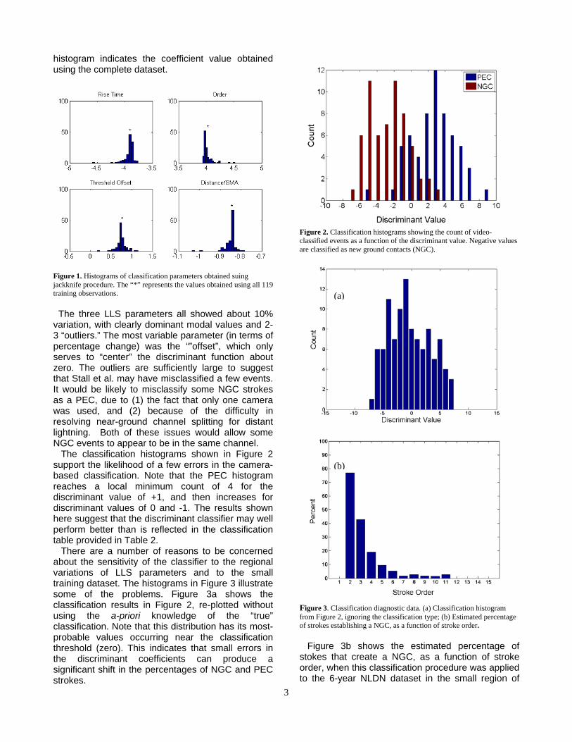
histogram indicates the coefficient value obtained using the complete dataset.

Figure 1. Histograms of classification parameters obtained suing jackknife procedure. The “*” represents the values obtained using all 119 training observations.

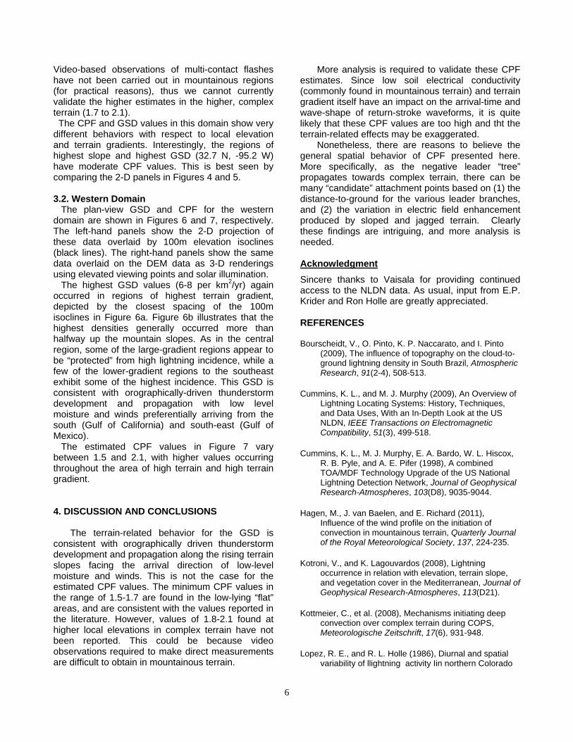
The three LLS parameters all showed about 10% variation, with clearly dominant modal values and 2-3 “outliers.” The most variable parameter (in terms of percentage change) was the “”offset”, which only serves to “center” the discriminant function about zero. The outliers are sufficiently large to suggest that Stall et al. may have misclassified a few events. It would be likely to misclassify some NGC strokes as a PEC, due to (1) the fact that only one camera was used, and (2) because of the difficulty in resolving near-ground channel splitting for distant lightning. Both of these issues would allow some NGC events to appear to be in the same channel. The classification histograms shown in Figure 2 support the likelihood of a few errors in the camera-based classification. Note that the PEC histogram reaches a local minimum count of 4 for the discriminant value of +1, and then increases for discriminant values of 0 and -1. The results shown here suggest that the discriminant classifier may well perform better than is reflected in the classification table provided in Table 2. There are a number of reasons to be concerned about the sensitivity of the classifier to the regional variations of LLS parameters and to the small training dataset. The histograms in Figure 3 illustrate some of the problems. Figure 3a shows the classification results in Figure 2, re-plotted without using the a-priori knowledge of the “true” classification. Note that this distribution has its most-probable values occurring near the classification threshold (zero). This indicates that small errors in the discriminant coefficients can produce a significant shift in the percentages of NGC and PEC strokes.

Figure 2. Classification histograms showing the count of video-classified events as a function of the discriminant value. Negative values are classified as new ground contacts (NGC).

Figure 3. Classification diagnostic data. (a) Classification histogram from Figure 2, ignoring the classification type; (b) Estimated percentage of strokes establishing a NGC, as a function of stroke order. Figure 3b shows the estimated percentage of stokes that create a NGC, as a function of stroke order, when this classification procedure was applied to the 6-year NLDN dataset in the small region of

(b)

(a)

4

southern Arizona. This region is the area used in both the original Stall et al. study and in the study of Valine and Krider. The percentage of second strokes creating an NGC (77%) is significantly higher than the 43% found by Valine and Krider. It is possible that the true percentage is higher than was found in those single-camera studies, but the magnitude of this difference suggests that the estimates to be provided in the following section should be interpreted with some caution. It should be noted that the analyses thus far -- including a review of the spatial pattern of Chi-square and SMA values -- show very little spatial variation within the 5x5 degree domains presented in this study. Thus it is likely that the spatial patterns of the number of ground-contacts-per-flash are potentially more robust than the absolute values. Future work will

both refine the classification method and better quantify the uncertainty. 3. RESULTS. In this section, negative ground stroke density (GSD) and the average number of ground contacts per flash (CPF) are presented for both the central and western domains. Each domain is presented separately, followed by an interpretation of the results. 3.1. Central Domain The GSD and CPF for the central domain are shown in Figures 4 and 5, respectively. The left-hand panels show the 2-D projection of these data overlaid by 100m elevation isoclines (black lines).

Figure 4. 6-year ground stroke density (GSD) for negative flashes near the Ozark Mountains. (a) Data overlaid by 100m isoclines. (b) viewed from an elevated viewing and, with solar illumination at that same angle.

Figure 5. 6-year average number of ground contacts per negative flash (CPF) for negative flashes near the Ozark Mountains, (a) overlaid by 100m isoclines, (b) viewed from an elevated viewing and, with solar illumination at that same angle.

5

The right-hand panels show the same data overlaid on the DEM data as 3-D renderings using elevated viewing points and solar illumination. The highest GSD values (12-15 per km2/yr) generally occurred in regions of highest terrain gradient, depicted by the closest spacing of the 100m isoclines in Figure 4a. Additional insight into the specific locations of the GSD maxima is provided in Figure 4b, showing high density in large areas of uniform slope and increasing altitude. Some of the large-gradient regions appear to be “protected” from high lightning incidence, while a few of the lower-gradient regions to the west and northwest (see

arrows) exhibit some of the highest incidence. This GSD is consistent with orographically-driven thunderstorm development and propagation with low level moisture and winds preferentially arriving from the south and south-east. The estimated CPF values in Figure 5 vary between 1.5 and 2.1, with higher values occurring throughout the area of high terrain and high terrain gradient. The lower CPF values in the range of 1.4-1.7, found in the low-lying areas, are consistent with the values reported in the literature [Stall et al.; Thottappillil et al.; Valine and Krider].

Figure 7. 6-year average number of ground contacts per negative flash (CPF) for negative flashes near the Rocky Mountains, (a) overlaid by 100m isoclines, (b) viewed from an elevated viewing and, with solar illumination at that same angle.

Figure 6. 6-year ground stroke density (GSD) for negative flashes near the Rocky Mountains. (a) Data overlaid by 100m isoclines. (b) viewed from an elevated viewing and, with solar illumination at that same angle.

6

Video-based observations of multi-contact flashes have not been carried out in mountainous regions (for practical reasons), thus we cannot currently validate the higher estimates in the higher, complex terrain (1.7 to 2.1). The CPF and GSD values in this domain show very different behaviors with respect to local elevation and terrain gradients. Interestingly, the regions of highest slope and highest GSD (32.7 N, -95.2 W) have moderate CPF values. This is best seen by comparing the 2-D panels in Figures 4 and 5. 3.2. Western Domain The plan-view GSD and CPF for the western domain are shown in Figures 6 and 7, respectively. The left-hand panels show the 2-D projection of these data overlaid by 100m elevation isoclines (black lines). The right-hand panels show the same data overlaid on the DEM data as 3-D renderings using elevated viewing points and solar illumination. The highest GSD values (6-8 per km2/yr) again occurred in regions of highest terrain gradient, depicted by the closest spacing of the 100m isoclines in Figure 6a. Figure 6b illustrates that the highest densities generally occurred more than halfway up the mountain slopes. As in the central region, some of the large-gradient regions appear to be “protected” from high lightning incidence, while a few of the lower-gradient regions to the southeast exhibit some of the highest incidence. This GSD is consistent with orographically-driven thunderstorm development and propagation with low level moisture and winds preferentially arriving from the south (Gulf of California) and south-east (Gulf of Mexico). The estimated CPF values in Figure 7 vary between 1.5 and 2.1, with higher values occurring throughout the area of high terrain and high terrain gradient. 4. DISCUSSION AND CONCLUSIONS

The terrain-related behavior for the GSD is consistent with orographically driven thunderstorm development and propagation along the rising terrain slopes facing the arrival direction of low-level moisture and winds. This is not the case for the estimated CPF values. The minimum CPF values in the range of 1.5-1.7 are found in the low-lying “flat” areas, and are consistent with the values reported in the literature. However, values of 1.8-2.1 found at higher local elevations in complex terrain have not been reported. This could be because video observations required to make direct measurements are difficult to obtain in mountainous terrain.

More analysis is required to validate these CPF estimates. Since low soil electrical conductivity (commonly found in mountainous terrain) and terrain gradient itself have an impact on the arrival-time and wave-shape of return-stroke waveforms, it is quite likely that these CPF values are too high and tht the terrain-related effects may be exaggerated.

Nonetheless, there are reasons to believe the general spatial behavior of CPF presented here. More specifically, as the negative leader “tree” propagates towards complex terrain, there can be many “candidate” attachment points based on (1) the distance-to-ground for the various leader branches, and (2) the variation in electric field enhancement produced by sloped and jagged terrain. Clearly these findings are intriguing, and more analysis is needed. Acknowledgment

Sincere thanks to Vaisala for providing continued access to the NLDN data. As usual, input from E.P. Krider and Ron Holle are greatly appreciated.

REFERENCES Bourscheidt, V., O. Pinto, K. P. Naccarato, and I. Pinto

(2009), The influence of topography on the cloud-to-ground lightning density in South Brazil, Atmospheric Research, 91(2-4), 508-513.

Cummins, K. L., and M. J. Murphy (2009), An Overview of Lightning Locating Systems: History, Techniques, and Data Uses, With an In-Depth Look at the US NLDN, IEEE Transactions on Electromagnetic Compatibility, 51(3), 499-518.

Cummins, K. L., M. J. Murphy, E. A. Bardo, W. L. Hiscox, R. B. Pyle, and A. E. Pifer (1998), A combined TOA/MDF Technology Upgrade of the US National Lightning Detection Network, Journal of Geophysical Research-Atmospheres, 103(D8), 9035-9044.

Hagen, M., J. van Baelen, and E. Richard (2011), Influence of the wind profile on the initiation of convection in mountainous terrain, Quarterly Journal of the Royal Meteorological Society, 137, 224-235.

Kotroni, V., and K. Lagouvardos (2008), Lightning occurrence in relation with elevation, terrain slope, and vegetation cover in the Mediterranean, Journal of Geophysical Research-Atmospheres, 113(D21).

Kottmeier, C., et al. (2008), Mechanisms initiating deep convection over complex terrain during COPS, Meteorologische Zeitschrift, 17(6), 931-948.

Lopez, R. E., and R. L. Holle (1986), Diurnal and spatial variability of llightning activity Iin northern Colorado

7

and central Florida during the summer, Monthly Weather Review, 114(7), 1288-1312.

Orville, H. D. (1965), A Photogrammetic study of initiation of cumulus clouds over mountainous terrain, Journal of the Atmospheric Sciences, 22(6), 700-&.

Orville, R. E., G. R. Huffines, W. R. Burrows, and K. L. Cummins (2011), The North American Lightning Detection Network (NALDN)-Analysis of Flash Data: 2001-09, Monthly Weather Review, 139(5), 1305-1322.

Pinto, O., I. Pinto, D. R. de Campos, and K. P. Naccarato (2009), Climatology of large peak current cloud-to-ground lightning flashes in southeastern Brazil, Journal of Geophysical Research-Atmospheres, 114.

Rudlosky, S. D., and H. E. Fuelberg (2010), Pre- and Postupgrade Distributions of NLDN Reported Cloud-to-Ground Lightning Characteristics in the Contiguous United States, Monthly Weather Review, 138(9), 3623-3633.

Schulz, W., K. Cummins, G. Diendorfer, and M. Dorninger (2005), Cloud-to-ground lightning in Austria: A 10-year study using data from a lightning location system, Journal of Geophysical Research-Atmospheres, 110(D9).

Stall, C. A., K. L. Cummins, E. P. Krider, and J. A. Cramer (2009), Detecting Multiple Ground Contacts in Cloud-to-Ground Lightning Flashes, Journal of Atmospheric and Oceanic Technology, 26(11), 2392-2402.

Thottappillil, R., V. A. Rakov, M. A. Uman, W. H. Beasley, M. J. Master, and D. V. Shelukhin (1992), Lightning subsequent-strokeelectric-field peak greater than the 1st stroke peak and multiple ground terminations, Journal of Geophysical Research-Atmospheres, 97(D7), 7503-7509.

Valine, W. C., and E. P. Krider (2002), Statistics and characteristics of cloud-to-ground lightning with multiple ground contacts, Journal of Geophysical Research-Atmospheres, 107(D20).