RESIN FILM INFUSION (RFI) PROCESS MODELING FOR … · MODELING FOR LARGE TRANSPORT AIRCRAFT WING...
168
RESIN FILM INFUSION (RFI) PROCESS MODELING FOR LARGE TRANSPORT AIRCRAFT WING STURCTURES Grant Number NAG-l-1881 Final Report Period of Performance: December 1, 1996 - December 31, 1997 Alfred C. Loos Aaron C. Caba Keith W. Furrow Department of Engineering Science and Mechanics Virginia Polytechnic Institute and State University Blacksburg, VA 24061 August 15, 2000 Prepared For: Mr. H. Benson Dexter NASA Langley Research Center Hampton, VA 23681 https://ntrs.nasa.gov/search.jsp?R=20000097377 2018-06-27T21:52:47+00:00Z
-
Upload
nguyendang -
Category
Documents
-
view
222 -
download
2
Transcript of RESIN FILM INFUSION (RFI) PROCESS MODELING FOR … · MODELING FOR LARGE TRANSPORT AIRCRAFT WING...
RESIN FILM INFUSION (RFI) PROCESSMODELING FOR LARGE TRANSPORT
AIRCRAFT WING STURCTURES
Grant Number NAG-l-1881
Final Report
Period of Performance: December 1, 1996 - December 31, 1997
Alfred C. Loos
Aaron C. Caba
Keith W. Furrow
Department of Engineering Science and Mechanics
Virginia Polytechnic Institute and State University
Blacksburg, VA 24061
August 15, 2000
Prepared For:
Mr. H. Benson Dexter
NASA Langley Research Center
Hampton, VA 23681
https://ntrs.nasa.gov/search.jsp?R=20000097377 2018-06-27T21:52:47+00:00Z

ABSTRACT
This investigation completed the verification of a three-dimensional resin transfer mold-
ing/resin film infusion (RTM/RFI) process simulation model. The model incorporates
resin flow through an anisotropic carbon fiber preform, cure kinetics of the resin, and heat
transfer within the preform/tool assembly. The computer model can predict the flow front
location, resin pressure distribution, and thermal profiles in the modeled part.
The formulation for the flow model is given using the finite element/control volume (FE/CV)
technique based on Darcy's Law of creeping flow through a porous media. The FE/CV
technique is a numerically efficient method for finding the flow front location and the
fluid pressure. The heat transfer model is based on the three-dimensional, transient heat
conduction equation, including heat generation. Boundary conditions include specified
temperature and convection. The code was designed with a modular approach so the flow
and/or the thermal module may be turned on or off as desired. Both models are solved
sequentially in a quasi-steady state fashion.
A mesh refinement study was completed on a one-element thick model to determine the
recommended size of elements that would result in a converged model for a typical RFI
analysis. Guidelines are established for checking the convergence of a model, and the
recommended element sizes are listed.
Several experiments were conducted and computer simulations of the experiments were
run to verify the simulation model. Isothermal, non-reacting flow in a T-stiffened section
was simulated to verify the flow module. Predicted infiltration times were within 12-20%
of measured times. The predicted pressures were approximately 50% of the measured
pressures. A study was performed to attempt to explain the difference in pressures.
Non-isothermal experiments with a reactive resin were modeled to verify the thermal mod-
ii

ule and the resin model. Two panelswere manufacturedusingthe RFI process.One was
a steppedpanel and the other wasa panelwith two 'T' stiffeners. The differencebetween
the predicted infiltration times and the experimentaltimes was4%to 23%.
o°o
111

Contents
1 Introduction
2
4
Literature Review
2.1 Flow .......................................
2.1.1
2.1.2
2.1.3
2.2
Analytical Methods ...........................
Fixed Mesh Methods ..........................
Moving Mesh Methods .........................
Heat Transfer ..................................
Theory
3.1 Flow Model ...................................
3.2 Heat Transfer Model ..............................
3.3 Resin Model ...................................
3.3.1 Cure Kinetics Sub-Model ........................
3.3.2 Viscosity Sub-Model ..........................
Finite Element Formulation
4.1 Galerkin Approximation ............................
iv
1
4
4
4
5
7
8
10
10
12
14
15
16
17
17

4.2
4.1.1 Flow Model ...............................
4.1.2 Thermal Model .............................
Finite Element/Control VolumeMethod ...................
4.2.1
4.2.2
4.2.3
4.2.4
4.2.5
Domain Discretization .........................
Resin Front Tracking ..........................
Flow Rate Calculation .........................
Fill Factor Calculations .........................
Time Step Calculation .........................
5 Computer Program
17
18
19
19
21
23
24
24
26
5.1 Pre-processing.................................. 26
5.2 Processor .................................... 28
5.3 Post-processing ................................. 31
5.4 Capabilities and Limitations .......................... 31
Material Characterization
6.1 3501-6ReducedCatalyst Resin Model ....................
Cure Kinetics Sub-Model ........................
Viscosity Sub-Model ..........................
Textile Preform Model .............................
6.2.1 Permeability ...............................
6.2.2 Compaction ...............................
6.1.1
6.1.2
6.2
7 Mesh Refinement Study
34
34
34
35
37
38
39
42

7.1 Flow and Thermal Model Considerations ................... 43
7.2 Model Description ............................... 43
7.2.1 Geometry ................................ 45
7.2.2 Boundary Conditions .......................... 45
7.2.3 Materials ................................ 47
7.3 Procedure .................................... 48
7.3.1 Description of the Finite Element Meshes............... 48
7.4 Thermal Error Calculations .......................... 49
7.5 Results ...................................... 53
7.5.1 Flow Model Convergence........................ 53
7.5.2 Thermal Model Convergence...................... 53
7.6 Discussion .................................... 62
7.7 Conclusions ................................... 63
7.8 Future Work ................................... 65
8 Flow Model Verification 66
8.1 Experiment ................................... 67
8.2 Simulation Model ................................ 70
8.2.1 Geometryand Boundary Conditions ................. 70
8.2.2 Permeability Calculation ....................... 72
8.2.3 MeshConvergence ........................... 73
8.3 Results ...................................... 75
8.4 Discussion .................................... 84
vi
8.4.1 Inlet Pressure .............................. 84
8.4.2 Skin, Flange,and Blade Pressures................... 84
8.4.3 Fill Times ................................ 85
9 Stepped Panel Simulation 87
9.1 Experiment ................................... 87
9.1.1 Preform and Tooling .......................... 87
9.1.2 Procedure ................................ 89
9.2 Simulation Model ................................ 91
9.2.1 Model Geometry ............................ 93
9.2.2 Boundary Conditions .......................... 96
9.3 Results ...................................... 106
9.4 Discussion .................................... 106
9.4.1 Temperatures .............................. 106
9.4.2 Fill Times ................................ 114
9.5 Conclusions ................................... 114
10 Two Stiffener Panel 115
10.1 Experiment ................................... 115
10.1.1 Preform and Tooling ........................ 115
10.1.2 Procedure ................................ 122
10.2 Simulation Model ................................ 122
10.2.1 Geometryand Mesh .......................... 122
vii

10.2.2 Boundary Conditions .......................... 126
10.2.3 Materials ................................ 127
10.3 Results ...................................... 131
10.4 Discussion .................................... 131
10.4.1 Temperatures .............................. 131
10.4.2 Fill Times ................................ 137
10.5 Conclusions ................................... 138
11 Conclusions and Future Work 139
11.1 Conclusions ................................... 139
11.2 Future Work ................................... 140
Bibliography 141
A Detailed Drawings of Tooling Components 144
A.1 SteppedPanel Tooling Schematics....................... 144
A.2 Two Stringer PanelTooling Schematics.................... 147
B Material Properties 153
B.1 Flow Properties ................................. 153
B.I.1 FVF ................................... 153
B.1.2 Permeability ............................... 154
B.2 Thermal Properties ............................... 155
B.3 MechanicalProperties ............................. 155
...
vnl

List of Figures
1.1 RFI setup .....................................
4.1 3-D control volume ................................
4.2 A typical element and the vectors used to calculate the areas of the sub-
volumes ......................................
4.3 Exploded view of an element showing the eight sub-volumes and their asso-
ciated vectors ...................................
4.4 Actual and numerical flow front .........................
5.1 3DINFIL program flowchart ...........................
5.2 Example of PATRAN post-processing capabilities ...............
6.1 In-plane permeability measurement fixture ...................
6.2 Through the thickness permeability measurement fixture ...........
7.1 Mesh refinement model .............................
7.2 Dimensions of the two stiffener preform ....................
7.3 Autoclave temperature cycle ..........................
7.4 Mesh for mesh refinement case A ........................
7.5 Mesh for mesh refinement case B ........................
2
2O
22
22
23
29
32
39
40
44
46
46
5O
5O
ix

7.6 Mesh for mesh refinement case C ........................
7.7 Mesh for mesh refinement case D ........................
7.8 Mesh for mesh refinement case E ........................
7.9 Temperature measurement points in the mesh refinement model .......
7.10 Thermal comparison
7.11 Thermal comparison
7.12 Thermal comparison
7.13 Thermal comparison
7.14 Thermal comparison
7.15 Thermal comparison
between the different meshes at point 1 .........
between the different meshes at point 2 .........
between the different meshes at point 3 .........
between the different meshes at point 4 .........
between the different meshes at point 5 .........
between the different meshes at point 6 .........
51
51
52
55
56
57
58
59
60
61
8.1 Flow verification preform dimensions ...................... 67
8.2 Flow verification preform dimensions ...................... 68
8.3 Pressure transducer locations .......................... 69
8.4 Quarter symmetry finite element mesh ..................... 71
8.5 Flow materials in the flow verification model ................. 72
8.6 Case A flow front progression .......................... 75
8.7 Case B flow front progression .......................... 76
8.8 Case C flow front progression .......................... 76
8.9 Inlet pressures for different meshes ....................... 77
8.10 Comparison between the measured and model predicted pressures at ports
l&4and2&=3 .................................
8.11 Comparison between the measured and model predicted pressures at ports
5 & 7 and 6 ....................................
78
79
X

8.12
8.13
8.14
8.15
Comparison between the measured and model predicted pressures at ports
8 & 9 and 12 ...................................
Comparison between the measured and model predicted pressures at ports
10 & 11 ......................................
Experimental and predicted infiltration times for the flow verification model.
Percent difference of wet out times for the flow verification model ......
8O
81
82
83
9.1 Dimensions of the stepped preform .......................
9.2 Tooling and layup of the stepped panel .....................
9.3 Locations of the thermocouples on the stepped preform ............
9.4 Locations of the FDEMS on the stepped preform ...............
9.5 Locations of the pressure transducers on the stepped preform ........
9.6 Initial one-element-thick finite element model .................
9.7 Final three-dimensional finite element model ..................
9.8 Measured autoclave temperatures during the stepped panel run .......
9.9 Applied temperature cycles for the initial model ................
9.10 Applied temperature cycles to the top of the final stepped model ......
9.11 Applied temperature cycles to the bottom of the final stepped model...
9.12 Temperature profiles at thermocouple location 1 for various convective coef-
88
89
90
91
92
94
95
97
98
98
99
ficients ...................................... 100
9.13 Temperature profiles at thermocouple location 2 for various convective coef-
ficients ...................................... 101
9.14 Temperature profiles at thermocouple location 4 for various convective coef-
ficients ...................................... 102
9.15 Temperature profiles at thermocouple location 5 for various convective coef-
ficients ...................................... 103
xi

9.16
9.17
9.18
9.19
9.20
9.21
9.22
9.23
9.24
Temperatureprofilesat thermocouplelocation 6 for variousconvectivecoef-ficients......................................
Temperatureprofilesat thermocouplelocation7 for variousconvectivecoef-ficients......................................
Comparison
Comparison
Comparison
Comparison
Comparmon
Comparison
Comparison
104
105
of thermal profilesat point 1................... 107
of thermal profilesat point 2................... 108
of thermal profiles at point 4................... 109
of thermal profiles at point 5................... 110
of thermal profiles at point 6................... 111
of thermal profiles at point 7................... 112
of predictedand measuredinfiltration timesfor the steppedpanel.113
10.1 Sketchof the two stiffenerpreform....................... 116
10.2 Tooling usedto infiltrate the two stiffener panel................ 117
10.3 Locationsof the FDEM sensorson the two stiffenerpanel.......... 118
10.4 Locationsof the pressuretransducerson the two stiffenerpanel....... 119
10.5 Locationsof the thermocoupleson the two stiffener panel.......... 120
10.6 Locationsof the thermocouplesmountedbeneath the baseplate and abovethe surfaceof the top tooling components................... 121
10.7 Meshusedin the initial model of the two stiffener panel. The model is oneelement thick in the Z direction......................... 123
10.8 Meshusedin the final model of the two stiffenerpanel............ 124
10.9 Sensorlocations in the finite elementmodel.................. 125
10.10Measuredautoclavetemperaturesusedin the two stiffener model...... 128
10.11Convectiveboundary conditions on the initial model............. 129
xii

10.12Convectiveboundary conditions on the final model.............. 130
10.13Materialsin the two stiffenerpanel....................... 130
10.14Flowfront progressionin the initial model................... 132
10.15Flowfront progressionin the final model.................... 133
10.16Measuredand predicted temperaturesat thermocouples2 and 4....... 134
10.17Measuredand predicted temperaturesat thermocouple5........... 135
10.18Predictedand measuredinfiltration times for the two stiffener panel.... 136
A.1 Baseplate..................................... 145
A.2 Detailed drawingsof the sensortap geometry................. 146
A.3 Baseplatefor the two stiffenerpanel...................... 148
A.4 Middle tool for the two stiffenerpanel..................... 149
A.5 Sensorlocations for the two stiffenerpanel................... 150
A.6 End tool for the two stiffener panel....................... 151
A.7 Shim for the two stiffenerpanel......................... 152
xiii

List of Tables
3.1 Values used to calculate the Graetz and Peclet numbers ........... 14
6.1 3501-6 reduced catalyst high temperature cure kinetics model constants. 35
7.1 Permeabilities applied to the mesh refinement model ............. 47
7.2 Size and run time of the models ......................... 48
7.3 Mesh parameters for case A ........................... 64
7.4 Mesh parameters for case C ........................... 64
8.1 Calculated fiber volume fractions of the T-section ............... 73
8.2 Three-dimensional flow model fiber volume fractions and permeabilities.. 74
9.1 Size and Run Time of the Models ........................ 96
10.1 Size and Run Time of the Models ........................ 122
10.2 Correspondence between the locations in the finite element model and the
physical sensors .................................. 125
10.3 Permeabilities applied to the two stiffener model ............... 131
xiv

Chapter 1
Introduction
The resin transfer molding (RTM) process is being explored as a cost effective method
for producing composite parts. RTM has several advantages over prepreg layup. First, a
near net shape dry preform is used. This eliminates the labor required to hand place each
layer of prepreg. Second, high dimensional accuracy of the finished part can be attained
because matched metal tooling is used. Finally, complex shaped components can be readily
fabricated. This allows for incorporation of many components into a single part and helps
to reduce the cost and weight of the structure [1].
The RTM process begins with a dry fiber preform. The preform is placed into a matched
metal mold and the mold is closed resulting in the compaction of the preform to the
specified fiber volume fraction. A liquid thermosetting resin is then injected into the mold.
The mold and resin can be preheated before injection, or the mold can be heated after
injection to cure the resin. To aid filling of the mold, a vacuum may be applied to remove
trapped air.
One of the requirements of the resin is that its viscosity must be low enough throughout the
process to fully infiltrate the preform. Since many of the resins currently in use were initially
Introduction
Vacuum Bag Bleeder Packs
Tools
Tool Tool Tool
%Preform
Tool
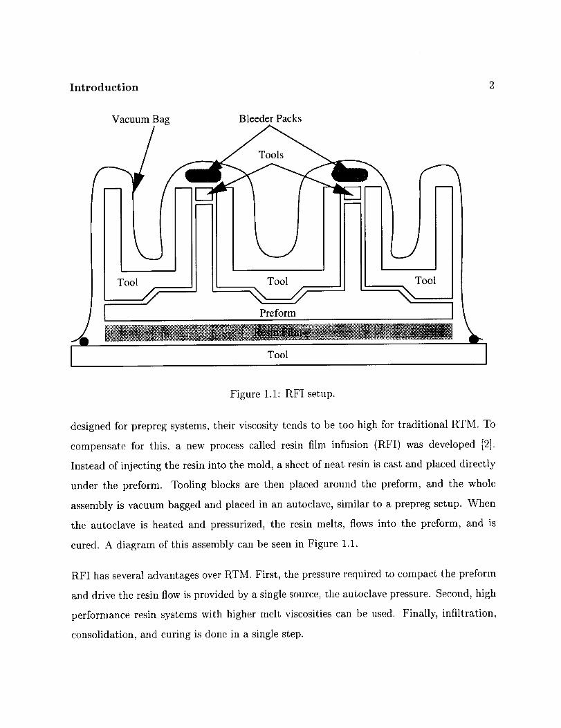
Figure 1.1: RFI setup.
designed for prepreg systems, their viscosity tends to be too high for traditional RTM. To
compensate for this, a new process called resin film infusion (RFI) was developed [2].
Instead of injecting the resin into the mold, a sheet of neat resin is cast and placed directly
under the preform. Tooling blocks are then placed around the preform, and the whole
assembly is vacuum bagged and placed in an autoclave, similar to a prepreg setup. When
the autoclave is heated and pressurized, the resin melts, flows into the preform, and is
cured. A diagram of this assembly can be seen in Figure 1.1.
RFI has several advantages over RTM. First, the pressure required to compact the preform
and drive the resin flow is provided by a single source, the autoclave pressure. Second, high
performance resin systems with higher melt viscosities can be used. Finally, infiltration,
consolidation, and curing is done in a single step.

Introduction 3
Due to the complex nature of the process,optimization of the RFI processcannot be
performed using conventionalexperimentation. The large number of variablesmakesthis
approachtime and cost prohibitive.
The objective of this work was to developand verify a comprehensivethree-dimensional
RTM/RFI simulation model. The model includes the effectsof flow through a three-
dimensionalanisotropic preform, heat transfer through the preform and surrounding tool-
ing, and cure kinetics of the resin. This model was usedto confirm the validity of using
measuredone-dimensionalpermeabilitiesasprincipal permeabilitiesin a three-dimensional
model. The model predictionswerealsocomparedto experimentaldata from both fiat and
T-stiffenedpanels.The model resultswerefound to be in goodagreementwith temperature
and flow front location measurements.
The program uses the finite element/control volume (FE/CV) method [3] to track the
flow of the resin through the preform. A time dependent finite elementschemeis used
to calculate the temperatures. The computer modelswere created in the PATRAN soft-
ware. Three-dimensionalmesheswerecreated and boundary conditions suchas specified
pressures,vent locations, and heat transfer coefficientswereapplied. Visualization of the
resultswasalso completedusing PATRAN.
In Chapter 2 a review of the literature detailing the current state of modeling efforts is
undertaken. The theory of the flow, heat transfer, and kinetics modelsused is discussed
in Chapter 3. The finite element formulations usedfor the flow and heat transfer models
arediscussedin Chapter 4. The RTM/RFI simulation program is discussedin Chapter 5.
Chapter 6 details the modelsusedfor the resin and fabric preform. Resultsfrom a thermal
meshrefinementstudy areshownin Chapter7. Comparisonsbetweenthe modelpredictions
and experimental results areshownin Chapters8-10.

Chapter 2
Literature Review
Previous studies have dealt with the modeling issues involved with RTM simulation. These
include models for the flow of the resin, the heat transfer, and the resin system used. A
survey of the current research in these areas will be presented in this chapter.
2.1 Flow
Flow of resin through the preform can be modeled as flow through a porous media. Many
studies use Darcy's law to describe the flow [3-7]. Modeling this flow is generally accom-
plished through one of four basic methods. These methods include analytical methods,
finite element, finite difference, and boundary element.
2.1.1 Analytical Methods
Analytical solutions for isothermal filling of simply shaped two dimensional molds have
been derived by Cai and Lawrie [8]. The mold is decomposed into simple geometric shapes

Literature Review 5
and these shapes are filled in succession. Within each section, one-dimensional flow is
assumed. Their equations give fill times of each section, and the pressure at the boundaries
between each section.
Boccard, Lee, and Springer [9] propose a graphical method for estimating fill times and vent
location in thin molds with arbitrary impermeable inserts. The measured and calculated
fill times generally agree within 10% and the predicted vent locations were close to the
measured vent locations.
Neither of these methods provides the exact location of the flow front within the mold,
only fill times are generated. Also, neither can be used if mold filling is non-isothermal
and anisotropic. The methods listed in the next two sections can provide data in these
situations.
2.1.2 Fixed Mesh Methods
The primary fixed mesh method used is the finite element/control volume (FE/CV) meth-
od. To use this method, the mold is first divided into finite elements. Around each nodal
location, a control volume is constructed by subdividing the elements into smaller volumes.
These control volumes are used to track the location of the flow front [1].
Many FE/CV implementations have been developed to model the resin flow in an RTM
process. Fraccia, Castro, and Tucker [3] implemented a FE/CV technique to model the
isothermal flow of resin in two-dimensional RTM molds. Predicted flow front locations
were compared to measured flow fronts in a two-dimensional mold. Fairly close agreement
was found. Several runs were also made with models of an automobile hood, and the effect
of gate location and in-plane permeability variation on the flow front advancement was
observed.

Literature Review 6
Voller and Peng [10] used a two-dimensional,isothermal volume of fluid approach. An
iterative solver is usedto determinethe fill factors for eachtime step. An arbitrarily large
time step can be used,and multiple volumescanbe filled in eachtime step. Results were
comparedto analytical solutionsand other numericalmethods. Their method agreeswith
both.
Gauvin et al. [6] implementedthe FE/CV techniqueto model isothermal flow in an RTM
subwayseat. Several'short shots' weremadewherethe mold waspartly filled with resin
and then allowedto cure. This wasintended to show the actual location of the flow front
in the mold. Comparisonof the model to the 'short shots' showeddiscrepanciesin the flow
front locations. Thesewere attributed to difficulty in predicting the permeability in the
corners where the preform was bent. They also noted that small local variations in the
permeability can havea large global effect.
A two-dimensional,isothermal,FE/CV modelwastestedby Calhounet al. [11]. A picture
framewith convergingflow to a centervent wasmodeled.A constant viscosity resin and a
constant velocity sourcewereused.The simulation time matchedthe experimentalfill time
within 1%. The pressuredata could only be matched through the useof various scaling
factors. The discrepancywasattributed to difficulties in measuringthe permeabilities.
Loos and MacRae [7] used a two-dimensionalRFI simulation with heat transfer and a
reactive resin to optimize the autoclavecycle for a T-stiffened panel. Both the preform
and the surrounding tooling weremodeled.The original cycle resultedin incompletefilling
of the part. Using the model, a suitable cure cyclewas found that resulted in complete
infiltration of the part.
Lee,Young, and Lin [12]havea two-and-a-half-dimensionalcodewhereflow is modeledas
two-dimensional and heat transfer is modeledas three-dimensional. A RTM automobile
hood with multiple cut-outs wassimulated. Pressurecontoursfor two different inlet po-

Literature Review
sitions wereshown. Flow front position wasalso usedto predict where weld lines would
form in the molded part.
Young [13]developeda three-dimensionalnon-isothermalmodelof the RTM process.For-
mulation for a wedgeelement is given. Simulation resultsare given for flow and cure in a
cubeand a T-section.
Loos et al. [14] havedevelopeda three-dimensionalnon-isothermalmodel of the RFI pro-
cess. A model of a T-stiffened panel with a variable thickness skin was compared to
experimental results. The model included both the preform and the tooling components.
Flow front location and degreeof cure were measuredusing frequency dependent elec-
tromagnetic sensors(FDEMS). Temperatureswere measuredusing thermocouples. Close
agreementwas found for the temperature,viscosity,and degreeof cure. Wet out occurred
simultaneouslyfor all FDEMS sensorson the surfaceof the skin, while the simulation pre-
dicted sequentialwet out. Discrepanciesbetweenthe predicted and measuredflow front
was attributed to premature wet-out of the FDEMS sensorsdue to resin flowing between
the preform and tool.
2.1.3 Moving Mesh Methods
Another method of tracking the flow is to have the numerical grid deform and move with the
flow front. One moving mesh method is the boundary element method. Yoo and Lee [15]
use the boundary element method to simulate a two-dimensional mold filling process. An
automatic meshing scheme was employed to track the flow front where the nodes on the
flow front move to track the shape of the front. When the nodes move, nodes that are close
to the mold boundary may move outside the mold wall. This will result in some mass loss
from the system as the fluid that has moved outside the wall is neglected. Viscosity of the

Literature Review 8
resin was isothermaland varied asa function of time only. Filling of a center-gatedsquare
mold and an 'L' shapedmold weresimulated. A small masslossof 3-4% was reported in
both cases.An advantageof this method is the accuracyof the flow front position sinceit
is determined exactly. Disadvantagesof this method include difficulty with multiple gates
and weld lines [15].
Another moving meshmethod is the body fitted coordinate method. This is a finite dif-
ferencemethod wherea curvilinear coordinate systemis fit onto the physical domain. An
irregular meshin the physical domain is convertedinto a regularmesh in the transformed
domain. Friedrichsand Giiqeri [5] useda two/three-dimensionalhybrid codeto model the
flow in a T-stiffened panel. The three-dimensionalformulation is only usednear wherethe
baseof the T joins the skin. The two-dimensionalcode is usedwhere out of plane flows
can be neglected,e.g. flow in the skin and stiffener away from the T joint. Results pre-
sentedinclude the computational meshesusedat varioustimes in the simulation, velocity
distributions, and tracer particle paths.
2.2 Heat Transfer
The energy balance in a single phase material is well understood, but the balance equations
for multi-phase systems are less readily available [16]. Two approaches are taken in the
literature. The first uses a single lumped temperature field for both the resin and preform.
In the second approach, separate governing equations are written for the resin and preform.
The two governing equations are coupled together through a heat exchange term of the
form [17]
q=hI(Tr-Tl) (2.1)

Literature Review 9
where q is the rate of heat exchange between the fiber and resin, hf is the heat transfer
coefficient between the fiber and resin, and Tf and Tr are the temperatures of the fiber and
resin, respectively. If the flow rates are fast, or the thermal gradients are large, the two
phase model is necessary to account for the finite heat transfer rate between the fiber and
resin. For slow flows, the resin and fiber temperatures will have time to equilibrate, and
only a single temperature model is necessary.
Lin, Lee, and Liou [18] performed non-isothermal molding experiments on a center gated
disc. For flow speeds of up to 12 cm/s they found better correlations with the two phase
model.
Loos et al. [14] state that in their RFI process model, the temperatures calculated for the
resin and fiber were almost identical, and a lumped model should be used. The reason
given was that the flow rates are very slow.

Chapter 3
Theory
The RFI and RTM processes consist of three concurrent phenomena: flow of the resin
through the preform, heat transfer through the tools and the preform, and curing of the
resin. Each of these is developed as a separate model in this chapter.
3.1 Flow Model
In any model of the RFI or RTM processes, one of the most important aspects is tracking
the flow of the resin through the preform. The three-dimensional flow model was developed
to calculate the pressure and velocity fields in the fluid and track the flow front position.
This formulation is patterned after Dav_ [4]. The assumptions made in the formulation of
the model include:
1. The preform is a heterogeneous, porous, anisotropic medium.
2. The flow is quasi-steady state.
3. Capillary and inertial effects are neglected (low Reynolds number flow).
10

Theory 11
4. The fluid is assumedto beNewtonian (its viscosity is independentof shearrate), and
incompressible.
5. The fluid doesnot leak from the mold cavity.
The continuity equation for the fluid canbe written as:
_Vi -o (3.1)Oxi
where vi is the interstitial velocity vector.
As the fluid flows through the pores of the preform, the interstitial velocity of the resin can
be written as:
(3.2)Vi _ -_
where qi is the superficial velocity vector and ¢ is the porosity of the solid. The porosity
was assumed to be constant in this investigation.
Using the assumptions that the preform is a porous medium and that the flow is quasi-
steady state, the momentum equation can be replaced by Darcy's law:
Sij OP (3.3)# Oxj
where # is the fluid viscosity, Sij is the permeability tensor of the preform, and P is the
fluid pressure.
Noting that the resin is incompressible and substituting (3.3) into (3.1) gives the governing
differential equation of the flow:
Oxi #

Theory 12
This second order partial differential equation can be solved when the boundary conditions
are prescribed. Two common boundary conditions for the inlet to the mold are either a
prescribed pressure condition:
or a prescribed flow rate condition:
Pint_t = Pi.let(t) (3.5)
Sij 0/' (3.6)Qn(t)=# Oxj
where Qn is the volumetric flow rate and n_ is the normal vector to the inlet. The boundary
condition along the flow front is taken to be one of zero pressure:
PIlowfront = 0 (3.7)
Since the resin cannot through the the mold wall, the final boundary condition necessary
to solve Equation (3.4) is that the velocity normal to the wall at the boundary of the mold
must be zero:
v.n=0 (3.s)
where fi is the vector normal to the mold wall.
3.2 Heat Transfer Model
In the RFI process, the heating rates and flow rates are small compared to the RTM or
SRIM processes. This allows a number of simplifying assumptions to be made in the ther-
mal analysis. First, the bagged preform and tooling assembly are heated in the autoclave at
a low heating rate, usually no greater than 5°C/min. During infiltration, the temperature
difference between the resin and the preform is small, thus the volumetric heat transfer

Theory 13
betweenthe resin and the preformcanbeneglected.Second,sincethe flow velocitiesof the
resinaresmall, heat transferdueto convectioncanbe ignored.This canbe expressedmath-
ematically with the Graetz and Pecletnumberslisted by Tucker [16]. The Graetz number
can be interpreted asthe flow direction convectiondivided by the transverseconduction.
The Graetz number is givenby Equation (3.9):
Gz- qh2 (3.9)c_tL
where q is the superficial resin speed, h is half of the mold thickness, L is the character-
istic flow length, and c_t is the total thermal diffusivity defined as (kzz/(pcp)), with kzz
representing the total effective conductivity in the thickness direction and p and % are the
density and specific heat of the resin, respectively.
The Peclet number can be interpreted as the ratio of dispersion to conduction, and is given
by Equation (3.10).
Pe = qd___£p (3.10)Ott
where dp is the diameter of a single fiber.
Using data from the two stiffener panel modeled in Chapter 10, the Graetz and Peclet
numbers were calculated. Table 3.1 lists the values used in the calculations. Since the
Graetz and Peclet numbers are <1, dispersion and convection can be neglected, and the
entire model can be described by one temperature field.
The heat transfer in the RFI process model is based on the three-dimensional transient
heat conduction equation, including a term for heat generation:
or o /kPCpot Oxi \ iJ-_xjJ- p/t/= 0 (3.11)
where p is the density, cv is the specific heat, kij is the thermal conductivity tensor for an
anisotropic material, and/:/is the heat generation due to exothermic chemical reactions.

Theory 14
Table 3.1: Valuesusedto calculatethe Graetz and Pecletnumbers.
Variable Value Unitskzz 0.51 W/(mK)
2h 0.01753 m
L 0.8255 m
dp 8 × 10 .6 m
q 2.58 x 10 -5 m/s
pCp 2.504 x 10⁶ J/(m3°C)
Gz 0.28
Pe 0.009
In order to solve Equation (3.11), the initial temperature distribution must be given:
T(_, 0) = T_.(_) (3.12)
where 2 is a position vector.
Boundary conditions for the solution of Equation (3.11) include:
Specified Temperatures:
Convection:
T(_,t) = Tspec(_,t)
k OT__J-g-gxj) _i = h(T_ - T)
Specified Flux: \ ij--_x j ] 72i : 0
[kInsulated: \ ij--_zj, ] ni = 0
where h is the convection coefficient and 0 is the specified flux.
(3.13)
(3.14)
(3.15)
(3.16)
3.3 Resin Model
The RFI process uses thermosetting polymeric resins. As the process progresses, the resin
begins to cure, change viscosity, and produce heat through exothermic chemical reactions.
Theory 15
A model is necessaryto predict the degreeof cureand the heat liberated from the curing
resin.
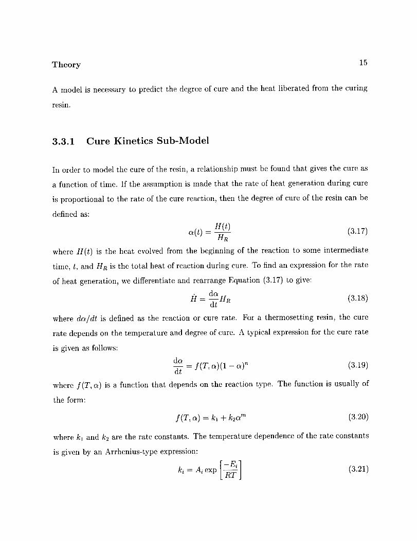
3.3.1 Cure Kinetics Sub-Model
In order to model the cure of the resin, a relationship must be found that gives the cure as
a function of time. If the assumption is made that the rate of heat generation during cure
is proportional to the rate of the cure reaction, then the degree of cure of the resin can be
defined as:
H(t) (3.17)oz(t)- HR
where H(t) is the heat evolved from the beginning of the reaction to some intermediate
time, t, and HR is the total heat of reaction during cure. To find an expression for the rate
of heat generation, we differentiate and rearrange Equation (3.17) to give:
dC_H (3.18)R
where da/dt is defined as the reaction or cure rate. For a thermosetting resin, the cure
rate depends on the temperature and degree of cure. A typical expression for the cure rate
is given as follows:
do
d---t= f(r, a)(1 _a)n (3.19)
where f(T, _) is a function that depends on the reaction type. The function is usually of
the form:
f (T, a) = kl -t- k2oLm (3.20)
where kl and k2 are the rate constants. The temperature dependence of the rate constants
is given by an Arrhenius-type expression:
Theory 16
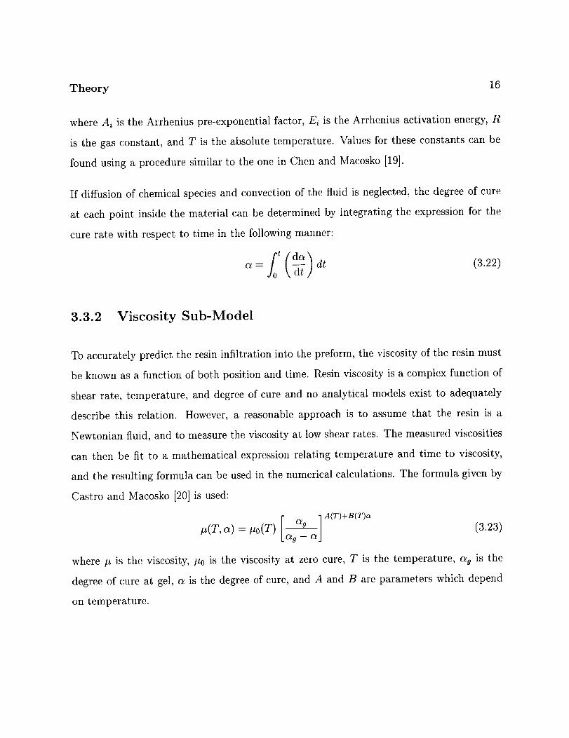
whereAi is the Arrhenius pre-exponential factor, Ei is the Arrhenius activation energy, R
is the gas constant, and T is the absolute temperature. Values for these constants can be
found using a procedure similar to the one in Chen and Macosko [19].
If diffusion of chemical species and convection of the fluid is neglected, the degree of cure
at each point inside the material can be determined by integrating the expression for the
cure rate with respect to time in the following manner:
a = dt (3.22)
3.3.2 Viscosity Sub-Model
To accurately predict the resin infiltration into the preform, the viscosity of the resin must
be known as a function of both position and time. Resin viscosity is a complex function of
shear rate, temperature, and degree of cure and no analytical models exist to adequately
describe this relation. However, a reasonable approach is to assume that the resin is a
Newtonian fluid, and to measure the viscosity at low shear rates. The measured viscosities
can then be fit to a mathematical expression relating temperature and time to viscosity,
and the resulting formula can be used in the numerical calculations. The formula given by
Castro and Macosko [20] is used:
#(T,_) = #o(T) _= 51A(T)+B(T)c_ (3.23)
where # is the viscosity, #0 is the viscosity at zero cure, T is the temperature, % is the
degree of cure at gel, c_ is the degree of cure, and A and B are parameters which depend
on temperature.

Chapter 4
Finite Element Formulation
Using the governing equations derived in Chapter 3, a finite element formulation is derived
for the flow and heat transfer models.
4.1 Galerkin Approximation
4.1.1 Flow Model
In Chapter 3, the governing equation for the flow model was found to be
Oxi Oxy = 0(3.4)
Using the procedure outlined by Reddy [21] the finite element formulation of Equation (3.4)
was found to be:
(4.1)
17

Finite Element Formulation 18
where
fa S_Z 0_ 0qJy df_Ki_ = e P Ox,_ Oz_
F[ = fn f kOidf_ + fre Qn kOidF
(4.2)
(4.3)
Here f2e is the domain of an element, Fe is the surface of an element, pie is the pressure at
each node, f is a volumetric source term, Q_ is a specified fluid flux through the face of
the element, and _i is a linear interpolation function.
4.1.2 Thermal Model
The governing equation for the transient heat transfer was found in Chapter 3 to be:
or 0 kij - p/:/= 0 (3.11)p cp Ot Ox_
Using the procedure outlined in Reddy [21] the finite element formulation was found to be:
[M_] {2/";} + [K_] {rj} = {F/} (4.4)
where
M/_ = fa p %_i_3 df_ (4.5)e
Ki_j = k,_.y_ Ox._ da + h _i_ y dF (4.6)e 1
F: = fr hT_k°idF+ fr _l_idF+_ p[-I_idft (4.7)1 2 e
Here, h is the convection coefficient, 0 is the specified flux through a face of the element,
and p/i/is the volumetric heat generation due to exothermic chemical reactions.
To solve Equation (4.4), a weighted average of the time derivative of the temperature at
two consecutive time steps is used [21]"
(1 - 0)2b_ + 0_b_+1 = T_+I - T_ (4.8)At_+l

Finite Element Formulation 19
A value of 0 = 0.887 was chosen because it gives good accuracy with reasonably sized time
steps [22].
4.2 Finite Element/Control Volume Method
In order to solve Equations (4.1) and (4.4) the domain of interest needs to be discretized
in both space and time. For the reasons stated in Chapter 2 a Finite Element/Control
Volume (FE/CV) approach was chosen for this study.
4.2.1 Domain Discretization
In order to track the moving flow front in the flow model, a technique is used that is based on
the assumption that each node in the mesh can be surrounded by a "control volume" that
is composed of a collection of sub-volumes from surrounding elements. The size and shape
of each control volume is determined by the number of nodes in each adjacent element.
This study used a structured mesh of 8-noded "brick" elements.
The flow domain is first discretized using finite elements, and then each element is further
divided into eight sub-volumes. Each sub-volume is associated with one of the nodes on the
element. The control volume for a particular node is composed of all of the sub-volumes
associated with that node. An example of a control volume composed of individual sub-
volumes is shown in Figure 4.1.
The flow calculations require the volume of the control volumes and the areas of the internal
faces of all sub-volumes. To find the areas, six vectors are constructed that start at the
centroid of the element and end at the center of each face of the element. These vectors

Finite Element Formulation 2O
Elements
Nodes
ControlVolume
II
I!
I
I
!
I
I
"I
I
I
I
Figure 4.1" 3-D control volume.
Finite Element Formulation 21
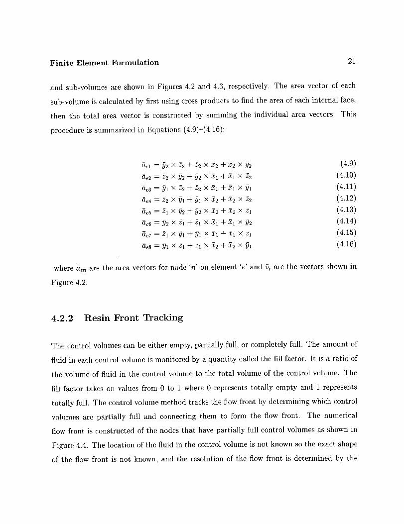
and sub-volumes are shown in Figures 4.2 and 4.3, respectively. The area vector of each
sub-volume is calculated by first using cross products to find the area of each internal face,
then the total area vector is constructed by summing the individual area vectors. This
procedure is summarized in Equations (4.9)-(4.16):
ael = _)2 × 22 + 22 × 22 + 22 × Y2 (4.9)
ae2 = 22 × Y2 + _)2 × 21 + 21 × 22 (4.10)
ae3 : Yl X 2 2 -Jr- 2 2 X 21 --[- 21 X Yl (4.11)
ae4 -_ Z2 X ?Jl -[- Yl x 2 2 -_- 2 2 x z2 (4.12)
ae5 _-_ Z1 X Y2 "[- Y2 X 2 2 -}- 2 2 X Z1 (4.13)
a'e6 _- Y2 X 21 -[- 21 X 21 -{- 21 X Y2 (4.14)
ae7 = 21 × _31+ Yl × 21 + 21 x 21 (4.15)
aes = 131× 21 + 21 x 22 + 22 × Yl (4.16)
where den are the area vectors for node 'n' on element 'e' and 9i are the vectors shown in
Figure 4.2.
4.2.2 Resin Front Tracking
The control volumes can be either empty, partially full, or completely full. The amount of
fluid in each control volume is monitored by a quantity called the fill factor. It is a ratio of
the volume of fluid in the control volume to the total volume of the control volume. The
fill factor takes on values from 0 to 1 where 0 represents totally empty and 1 represents
totally full. The control volume method tracks the flow front by determining which control
volumes are partially full and connecting them to form the flow front. The numerical
flow front is constructed of the nodes that have partially full control volumes as shown in
Figure 4.4. The location of the fluid in the control volume is not known so the exact shape
of the flow front is not known, and the resolution of the flow front is determined by the

Finite Element Formulation 22
n4 n3
n8
Y
_ .-"nl _2 _/// n2 _ X
Zn5 n6
Figure 4.2: A typical element and the vectors used to calculate the areas of the sub-volumes.
-X5 xl z-5 _5
;--t--2_"" !,,I y2 n2
n_" n6 y2 y2
Figure 4.3: Exploded view of an element showing the eight sub-volumes and their
associated vectors.

Finite Element Formulation 23
I .... I
,' • ,' EmptyCVI I
I .... I
Partially Full CV
Full CV
Actual Flow Front
unhurt• Numerical Flow• Front
Figure 4.4: Actual and numerical flow front.
mesh density. A detailed discussion of flow front recovery can be found in [23].
4.2.3 Flow Rate Calculation
Once the domain has been discretized, the pressures in the preform must be calculated.
The boundary conditions listed in Equations (3.5)-(3.8) must be applied. To approximate
the zero pressure boundary condition at the actual flow front, the nodes on the numerical
flow front have their pressures set to zero. Next, the other boundary conditions such as
specified pressure and specified flow rate are applied, and then Equation (4.1) is solved to
find the pressure distribution in the preform.
After the pressures have been calculated, the velocities are calculated at the centroid of

Finite Element Formulation 24
each element using Darcy's law:
1 S_j OP
vi- ¢ _ Oxj
It is assumed that the velocity of the fluid is constant throughout each element.
(4.17)
The flow into each nodal control volume from each element can be found with:
Qe. = 9e. a_n (4.18)
where Q_n is the volumetric flow rate into control volume (n) from element (e), _ is the
fluid velocity in the element, and g_ is the area vector for the sub-volume as calculated in
Section 4.2.1.
4.2.4 Fill Factor Calculations
After the flow rates into each control volume have been calculated the fill factors can be
updated. Given the current time step, the fill factors from the previous step, the calculated
flow rate, and the volume of each CV, the new fill factors can be calculated with:
AtE Q . (4.19)ft+'= ft+ v.
where fn is the fill factor, At is the time step, V, is the volume of the control volume, and
the superscripts indicate time level.
4.2.5 Time Step Calculation
The time step for the next iteration must be calculated before the solution can proceed.
The optimal time step would be where the fluid just fills one control volume. If a larger

Finite Element Formulation 25
step were chosen, the flow front would over-run the control volume and a loss of mass from
the system would result. The time to fill the partially full control volume 'n' is calculated
with the following relation:
At_ - (1- f_)V_ (4.20)EeQe_
Once At,_ has been calculated for all the partially full control volumes, the smallest Atn is
chosen as the time step for the next iteration.

Chapter 5
Computer Program
Using the theory developed in Chapter 3 and the finite element formulations developed in
Chapter 4, a computer program called 3DINFIL was written to simulate the RTM/RFI
process. This chapter will discuss pre-processing, processing, and post-processing of a
model.
5.1 Pre-processing
The computer program requires three input files. The first file contains the flow model,
the second contains the thermal model, and the third contains the parameters necessary
to run the simulation.
The finite element model is constructed using 8-noded hexahedral brick elements. PATRAN
was used to create the model files. The PATRAN model consists of geometry, a finite
element mesh, materials, and boundary conditions. First the geometry is constructed
and meshed. Then material properties are defined and boundary conditions are applied.
Finally the model is saved in PATRAN 2.4 neutral file format. The program requires that
26
Computer Program 27
the model files be in PATRAN neutral file format.
For the flow model, only the preform regionand possiblyany bleederpacksareconsidered.
The material properties required are the three-dimensionalpermeability tensors of the
preform and bleeder packs. Allowable boundary conditions include: specified pressure,
vent locations, specifiedflow rates, and pressurecycle flags. Also, any initially filled nodes
arespecified. If multiple injection ports are used,different pressurecyclescanbe supplied
for eachinjection port. Pressurecycleflagsareusedto determinewhich cycle is applied to
the element.
The secondmodel is the heat transfer model. This model includes the preform and any
tooling that surrounds it. The three-dimensionalthermal conductivity tensors of each
material must bespecified.A temperaturedistribution is input asthe only initial condition.
The boundary conditions include either convectivecoefficientsor specifiedtemperatures,
and temperature cycle flags. The codewill accept multiple temperature cycles,and the
cycle flags specify which cycle is applied to which element. Only one type of thermal
boundary condition is allowedin eachmodel. The model must haveeither convectivetype
boundary conditions or specifiedtemperature boundary conditions.
Both the flow and heat transfer models must use the samemesh in the preform region.
When building thesetwo modelscaremust be taken to ensurea one-to-onecorrespondence
between the nodes and elements in the flow model and the nodes and elements in the
preform regionof the heat transfer model.
The third file that must be createdis the 3dinit. ±np file. This file containstime limit and
iteration limit specifications,the initial viscosity,and the pressureand temperaturecycles.

Computer Program
5.2 Processor
28
The processor is composed of the three sub-models: the flow model, the heat transfer
model, and the resin model. All three models are coupled and non-linear. The flow model
needs the viscosity from the resin model, the resin model needs the temperatures from
the heat transfer model, and the heat transfer model uses the heat generation from the
resin model. Instead of trying to directly solve this system, the sub-models are solved
sequentially. In addition, each sub-model is solved in a piecewise linear fashion. This not
only reduces the coding and solution effort, it allows the code to be in a 'modular' form,
with each sub-model in its own module. This way each module can be turned on and off
individually depending on the particular analysis being performed.
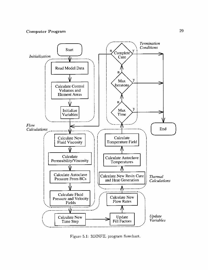
The program is divided into six sections:
1. Initialization
2. Flow Calculations
3. Update Variables
4. Thermal Calculations
5. Termination Conditions
6. Final Output and Exit
Each section performs its calculations and passes necessary information on to the other
sections. A flow chart of the program is shown in Figure 5.1.
The initialization section begins by reading the three files created during pre-processing:
the flow model, thermal model, and processing cycle. After the finite element information
has been read from the model files, the code calculates the control volumes as discussed in
Section 4.2.1. Also included in this section of the code is initialization of variables, including
Computer Program 29
Initialization ( Start,i,
I Read Model Data
Calculate ControlVolumes and
Element Areas
iii|Ji||i|iiR
eI Initialize ], Variables
-. ............. J---............ .*Flow II
Calculations .............. q/.-. ............ .
J'Calculate NewFluid Viscosity
q/
I CalculatePermeability/Viscosity
q/Calculate AutoclavePressure From BCs
n
Calculate [Temperature Field
Calculate Autoclave
Temperatures
Calculate New Resin Cureand Heat Generation
[ Calculate Fluid ] , *'" I I ',, Calculate New ,
[ Pressure and Velocity [ _ [ [I Fields I "* ! [ Fl°wRates I
::::::::::::::::::::::::::::::::::::::
": Calculate New Updatei
: Time Step Fill Factors *
Termination' Conditions
f
f
f
ThermalCalculations
UpdateVariables
Figure 5.1: 3DINFIL program flowchart.

Computer Program 3O
assigningan initial degreeof cure to eachnode, assigningthermal material properties to
all elements,and assigningpermeabilitiesand porosities to the preform elements.
Once the initialization sectionis complete,the code beginsthe main iteration loop. The
first section in this loop containsthe flow calculations. The purposeof this section is to
calculate the pressurefield in the preform using the viscosity, permeability, and applied
pressure. The viscosity at eachnode and in eachelement is calculated using the current
temperature and degreeof cure. All referencesto permeability in Equation (4.2) havethe
permeability divided by the viscosity,so this quantity is calculatedand recordedfor each
element that has fluid in it. Next, the autoclavepressureis calculated from the profile
given in the 3dinit. inp file and this pressureis appliedto the preformwherethe pressure
cycle flags were applied. Finally, the boundary conditions are applied, and the pressure
field is calculated usingEquation (4.1).
To savestorage space,the stiffness matrix [Kij in Equation (4.1)] is stored in a sparse
storage format. The code currently usesthe NASA Vector SparseSolver (VSS) to solve
the equations[24].
Oncethe pressurefield hasbeencalculated,the pertinent modelvariablesmust beupdated
for the next iteration. The flow rates are found and the fill factors are updated. Next, a
new time step is calculatedfor the next iteration.
In the thermal calculation section,the codecallsthe curesubroutine to calculatethe degree
of cure of the resin, and the rate of heat generation. The codethen calculatesthe current
autoclave temperatures,basedon the thermal cycle profiles input in the 3dinit. inp file.
Finally, the boundary conditions areappliedand the temperaturefield is calculated. Since
the equation usedto solvefor the temperaturefield, Equation (4.8), containsthe time step,
the massmatrix (Mij) and the thermal stiffnessmatrix (Kij) must be recalculated each
time step.

Computer Program 31
Similar to the flow computations, the stiffness matrix is stored using a sparsestorage
format, and the solution is found with the NASA VSSsolver.
Finally, the codechecksto seeif any programtermination conditions havebeenmet. Con-
ditions that will causethe codeto end calculationsare reachingthe maximum simulation
time, maximum iterations, or completecure of the resin. If any of theseconditions are
met, the codeexits, otherwiseanother iteration begins.
While the code is running, results are written to disk. This allows the user to check
the progressof the solution, and prevents complete loss of information in the event of
a computer crash. After the calculations are complete, the program writes a PATRAN
sessionfile that the usercan run to automatically load the results into PATRAN.
5.3 Post-processing
PATRAN was used to post-process the results from the simulation runs. An example of
the PATRAN output is shown in Figure 5.3.
5.4 Capabilities and Limitations
Since the program was written in standard Fortran 77, it has proven to be easily portable
to different computers and operating systems. Currently, the code has been successfully
ported to Silicon Graphics, HP, and Cray computers.
The code has been written in a modular form. As new resin systems are characterized,
they can be easily added to the model. Experience has shown that a significant amount
of the run time is spent in the solver subroutines. As faster or machine specific solvers

Computer Program 32
MSC/PATRAN Version 6.0 05-Sep-97 17:29:04
FRINGE: t-sec/verify/case3, 3dflowptnod: Flow Front Position -PATRAN 2.5
Y
8890.
8298.
7705.
7112.
6520.
5927.
5334.
4741.
4149.
3556.
2963.
2371.
1778.
1185.
592.7
0.
Figure 5.2: Example of PATRAN post-processing capabilities. This figure shows the flow
front progression in a center port injected, T-stiffened model. The color bands represent
the flow front location at different times. The units are in seconds.

Computer Program 33
become available, the solver can easily be replaced by changing a few lines of code.
As with any simulation program, without correct inputs, correct results cannot be expected.
The many variables that are required by this simulation model must be accurately specified
before this simulation model can be used in a predictive capacity. Some of these variables
include material models such as the kinetics and viscosity models, and the permeability and
compaction models. Other variables include the material properties such as conductivity
and heat capacity. Another set of variables include accurate specification of the boundary
conditions including pressure and thermal cycles. The following chapters will show how
the code was verified and list the constants used.

Chapter 6
Material Characterization
The computer program described in Chapter 5 cannot accurately model the RTM/RFI
process without accurate inputs. This chapter discusses how the 3501-6 reduced catalyst
resin and the carbon-fiber textile preforms were characterized.
6.1 3501-6 Reduced Catalyst Resin Model
The resin studied here is the Hercules 3501-6 resin system. It is a high performance epoxy
based system widely used in the aerospace industry. In the current study, only half of
the recommended amount of catalyst was added. This was done to increase its processing
"window" where the viscosity of the resin is low enough to allow infiltration of the preform.
6.1.1 Cure Kinetics Sub-Model
Isothermal and dynamic differential scanning calorimetry (DSC) were used to measure the
cure reaction kinetics of the reduced catalyst resin. Isothermal measurements were made
34

Material Characterization 35
Table 6.1:3501-6 reducedcatalyst high temperaturecure kinetics model constants.
] ValueA1 2.516 x l0 s
A2 40.35097
A3 8.7355 x 10⁷
E1/R 10.90214
E2/R 5.28071
E3/R 11.2061
nl 0.8817
n2 (0.029598T) - 3.28439m 0.96398
C1 0.05
6;'2 0.95
HR 430.0
p 1260
Units
sec -I
sec -I
sec- 1
Kelvin
Kelvin
Kelvin
T in Kelvin
kJ/kg
kg/m 3
between 110 and 165°C. The complex curing reaction for this resin was resolved into two
independent nth order reactions, and the data were fit to a two part mathematical model:
do_-- Clkl(1 -o!) m @ C2(k2 -t- k3c_m)(1 _a)n2 (6.1)
dt
p/:/ do_ (6.2)- dt pHR
where
(6.3)
The experimentally determined values for all the constants are listed in Table 6.1.
6.1.2 Viscosity Sub-Model
The viscosity-time characteristics of the reduced catalyst resin were measured at elevated
temperatures using a Bohlin rheometer. Viscosity measurements were made using 25 mm

Material Characterization 36
diameter parallel plates. An appropriate quantity of resinwasusedin order to maintain a
plate gap of 1-2 mm. The cure reaction kinetics modelwasusedto convert the isothermal
viscosity-time curvesto viscosity-conversioncurves.For temperaturesabove90°C the resin
viscosity wasfound to fit the following equationfrom Chapter 3:
#(T, a) = #o(r) (3.23)
where
#0=7.875×10-l°exp[7_ --65]- TinKelvin
A = 4.151
B = -17.831 + 0.147 T T in °C
where # is the viscosity in Pa.s, and a is the degree of cure.
Since the heating rates used to heat the composite/tool assembly in the RFI process are
slow, the resin flow and complete wet out often occurs before the autoclave reaches 90°C.
These unique processing conditions required the development of a low temperature viscosity
model. A Brookfield viscometer was used to perform isothermal viscosity measurements
between 60 and 90°C. The cure of the resin was also measured by DSC at temperatures
below 90°C, and it was found that the advancement of the resin was no more than 5-8% for
times up to 8 hours. To fit the data, it was assumed that there is no significant cure below
90°C, and the viscosity in the low temperature region depends only on the temperature.
The data were fit to an Arrhenius model:
#(T)=4.0074×10⁻¹⁶exp[12_ -4"9]- (6.4)
where p is the viscosity in Pa-s and T is the temperature in Kelvin.

Material Characterization
6.2 Textile Preform Model
37
Two general types of textile preforms were characterized. The first is a multiaxial warp
knit fabric that contains seven layers of unidirectional carbon fibers The seven layers are
knitted together with polyester thread. The knitted unit is referred to as a "stack". The
carbon fibers are arranged so that each stack has quasi-isotropic mechanical properties.
Two different types of carbon fibers were used in this type of preform: AS4 and Tenax.
Details about the warp knit fabric can be found in [25-27]. The second type of fabric is a
triaxial braided carbon fiber preform. The tows are braided around a cylindrical mandrel
to form a tube. The tubes were fabricated with AS4 6k carbon fiber bias yarns at a braid
angle of 60 ° and with IM7 36k carbon fiber axial yarns. Approximately 44% of the fibers
were in the axial direction and 56% of the fibers were in the off-axis directions. The tube
is flattened to form an individual layer.
To form a preform, the stacks or tubes of material are cut to the desired dimensions and
stacked together. The material is then stitched through the thickness using a modified lock
stitch and Kevlar thread. The stitch rows on all material tested were 0.2 inches apart and
the stitch step was 1/8 inch.
The computer model requires the permeability and the fiber volume fraction of these textile
preforms as input. This section describes the methods used to find models that can predict
the permeability and fiber volume fraction given the pressure applied to the preform. The
types of preforms tested were 8 stack warp knit, and 4 and 14 tube braid.

Material Characterization
6.2.1 Permeability
38
There are two common methods for measuring the permeability of fabrics and preforms.
The two methods are steady-state and advancing front measurement. The materials used in
this study were characterized using steady state measurements. Steady-state permeability
is measured after the preform has been saturated, and is carried out under constant flow rate
injection. The pressure differential across the preform is measured and the permeability is
calculated from Darey's Law. The permeability is measured as a function of fiber volume
fraction. Both in-plane and through-the-thickness permeabilities were measured. Flow
rate, mold height and pressure data were gathered using a National Instruments data
acquisition system controlled by LabVIEW software. A complete description of the system
can be found in Fingerson [28].
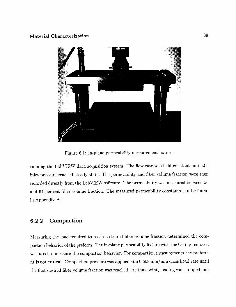
Figure 6.1 is a picture of the in-plane permeability fixture. Fingerson, Loos, and Dexter [28]
contains detailed drawings of the permeability fixture. The mold cavity is 17.78 cm long
by 15.32 cm wide. The preform is 15.2 cm long by 15.32 cm wide. The extra cavity length
forms an inlet manifold allowing even inlet pressure across the face of the preform.
Figure 6.2 is a sketch of the through-the-thickness permeability fixture set up. The fixture
is described in Weideman [29] and Hammond et al. [30]. The fixture test section was
designed to characterize 5.1 cm long by 5.1 cm wide fabric preform samples. The upper
and lower surfaces of the mold cavity compress the preform and contain holes to allow for
fluid flow through the thickness of the preform.
For each fixture, specimens were cut out of the preform with a band saw so that the
specimen fit tightly in the mold. The fixture was then closed and the mold height and
compaction pressure were measured. Fluid was pumped through the preform using a Parker
Zenith precision Gear Metering Pump. The entire pump system communicates with the PC
Material Characterization 39
Figure 6.1: In-plane permeability measurement fixture.
running the LabVIEW data acquisition system. The flow rate was held constant until the
inlet pressure reached steady state. The permeability and fiber volume fraction were then
recorded directly from the LabVIEW software. The permeability was measured between 50
and 64 percent fiber volume fraction. The measured permeability constants can be found
in Appendix B.
6.2.2 Compaction
Measuring the load required to reach a desired fiber volume fraction determined the com-
paction behavior of the preform. The in-plane permeability fixture with the O-ring removed
was used to measure the compaction behavior. For compaction measurements the preform
fit is not critical. Compaction pressure was applied at a 0.508 mm/min cross head rate until
the first desired fiber volume fraction was reached. At that point, loading was stopped and

Material Characterization 40
Flow Out
Flow In
Figure 6.2: Through the thickness permeability measurement fixture.

Material Characterization 41
the load level required to achieve equilibrium was recorded. Relaxation occurs in the pre-
form as the fibers realign themselves under the applied load. Again compaction loads were
recorded between 50-64% fiber volume fraction. The same data acquisition system used
for the permeability test was in the compaction experiments. The measured compaction
constants can be found in Appendix B.

Chapter 7
Mesh Refinement Study
There are many variables that can affect the accuracy of a finite element model. One class
of variables is the user inputs to the model. Inaccurate material properties or inaccurate
boundary condition application can result in meaningless results. Another user input that
is important to the accuracy is the discretization of the physical problem. In many models,
the solution may have high spatial gradients in some areas. The discretization must be fine
enough to adequately capture these gradients. Different solutions exist to capture these
gradients. One method is to increase the order of the element used. Instead of using a linear
element, a quadratic, a cubic, or higher order element can be used. The other method is
to decrease the size of the elements in the area. As the element order increases or the size
of the elements decrease, the finite element solution will converge to the "true" solution of
the problem [21].
The purpose of this study was to find the minimum recommended element sizes that result
in a converged model for a typical RFI part. The results reported here are intended as
a starting point when checking convergence of any model and are not intended as hard
and fast rules. It must be stressed that failure to check each finite element model for
convergence can result in inaccurate and flawed results.
42

Mesh Refinement Study
7.1 Flow and Thermal Model Considerations
43
3DINFIL is composed of a flow model and a thermal model. Each model requires separate
considerations when checking for convergence. This section will discuss issues that may
arise in each model.
The flow model has two main variables that are of interest. The first is the fluid pressure,
and the second is the flow front location. The fluid pressure accuracy is determined by the
mesh resolution in the direction of the pressure gradients. Pressure gradients will typically
be highest around sharp geometry transitions such as injection ports (in the case of RTM)
or the blade/flange transition region. The resolution of the flow front location will be
determined by the distance from one node to the next. Since the control volume method
does not locate the flow front exactly, the uncertainty in the flow front locations is the
length of the element.
In the thermal model, there is only one variable, the temperature. One area where high
temperature gradients can form is where materials of different thermal conductivities are in
contact with each other. Another area that will have high gradients will be the boundary
of the model where the convective boundary conditions are applied.
7.2 Model Description
A two stiffener panel was chosen to be modeled in this study because it is typical of the
stiffened wing skin parts to be modeled. The geometry is representative of a full scale RFI
part, and the same materials are used in both the model and an actual part. Also, the two
stringer panel incorporates the latest hogged-out tooling concept. A sketch of the model is
shown in Figure 7.1.

Mesh Refinement Study 44
Y
t
Preform Blade
End Tool
X
Shim
Bottom Plate
Plane of Symmetry
Center Tool
Resin Film
Figure 7.1: Mesh refinement model.

Mesh Refinement Study 45
The finite element model used in the study was one element thick in the Z direction.
This was chosen for two reasons. First the one element thick model will simulate a two-
dimensional slice of the part. Since the two stringer panel was long compared to the
thickness of the skin, this seems to be a valid assumption. Also, many parts can be initially
modeled as two-dimensional. The second reason is that the mesh refinement is easier in
the two-dimensional model than in a full three-dimensional model. In a model of a slice of
the part, the temperature fields are easier to visualize. The run times are also much faster
than a full three-dimensional model.
The results that are found for the one element thick model should be useful as a starting
point for three-dimensional mesh refinement study.
7.2.1 Geometry
Approximate dimensions of the preform are shown in Figure 7.2.
tooling components can be found in Appendix A, Section A.2.
The dimensions of the
7.2.2 Boundary Conditions
The boundary condition on the flow model was the autoclave pressure. A pressure of 791
kPa (114.7 psi) was applied to the bottom surface of preform where the resin film is located.
The boundary conditions on the thermal model consisted of convective boundary con-
ditions. The autoclave temperature is shown in Figure 7.3. Convective coefficients of
50 W/(m2.°C) were applied to the outer surfaces of the model. No convection coefficients
were applied to the front or back surfaces of the model, or to the plane of symmetry. These
surfaces were taken to be thermally insulated.

Mesh Refinement Study 46
l 1.169 cm 0.889 cm
lOi1
19.51I
w |
I|
Ii
Iii|
I
ii
1 cm
/
45.872 cm
._1
1.753 cm
[ _-_ 3.429 cm
cm-- I \1
/
-I
Figure 7.2: Dimensions of the two stiffener preform.
200
180
160
140
_ 120
_ 100E
_- 80
6O
4O
Autoclave Temperature CycleI I I
2ihour hold
i i i _ 2.8 C/min tamp to 177i C
i 2hour hold / ::
:6 C)min iampto i2i C ..........................................
¢
20 i i i i i i0 50 1O0 150 200 250 300
Time (min)350
Figure 7.3: Autoclave temperature cycle.

Mesh Refinement Study 47
Table 7.1: Permeabilities applied to the mesh refinement model.
Material Permeability m 2
Skin: Warp Knit 57% FVF
IPP (Szz)
IPN (Sxx)
TTT (Sy_)Blade: 14 Tube Braid 570-/0 FVF
IPP (Szz)
IPN (Sy_)
TTT (Sx_)
1.031 x 10 -11
1.047 x 10 -12
3.665 x 10 -12
1.348 x 10 -11
6.914 x 10 -12
7.417 x 10 -13.
* No 14 tube data available, computed using 4 tube braid TTT fit.
7.2.3 Materials
There were two flow materials used in the model, one for the blade and one for the skin
and skin/flange regions. The preform fiber volume fraction was chosen to be 57%, and
the permeabilities were calculated using the constants in Appendix B. The constants are
given for permeabilities as in-plane, parallel to the stitching, (IPP); in-plane, normal to
the stitching (IPN); and through-the-thickness (TTT). The materials were applied to the
model as shown in Figure 7.1, and the permeability values are shown in Table 7.1
The thermal materials used were 6061-T6 aluminum and the carbon fiber preform. The
material constants are listed in Appendix B. The aluminum is isotropic, so no orientation
is necessary. The preform is thermally orthotropic, so the orientation of the conductivity
tensor is necessary. For the skin, the in-plane value was used for k_x and kzz and the TTT
value was used for kyy. The blade used the in-plane value for kyy and kzz and the TTT
value for k_.

Mesh Refinement Study 48
Case
A
B
C
D
E
Table 7.2: Size and run time of the models.
Flow Model Thermal Model CPUTime
Nodes Elements Nodes Elements (min)
708 302 1324 601 2.7
604 252 1168 521 2.2
1008 434 2122 970 4.6
1814 792 4270 1998 12.4
6166 2856 15902 7680 126.6
7.3 Procedure
In this study, a very fine mesh was used to find the "true" solution. The other, coarser,
meshes were compared against this. In the real world this option is usually not available
due to time and size limitations. The general procedure for finding a converged mesh is as
follows:
1. Run the first coarse mesh.
2. Refine the mesh.
3. Compare the results from the refined mesh with the old mesh, and determine error
between the two.
4. If the error is too high, repeat steps 2 and 3 until the error is acceptable.
7.3.1 Description of the Finite Element Meshes
The five meshes used are shown in Figures 7.4-7.8. The number of nodes and elements in
each model is listed in Table 7.2.

Mesh Refinement Study 49
CaseA wasbasedon a McDonnell DouglasAircraft (MDA) mesh refinementstudy done
to find the necessarymeshdensity for a convergedflow model. Thermal convergencewas
not checkedin the MDA study.
CaseB was constructed to determine a lower limit on the number of elementsthat are
necessarythrough the thicknessof the stiffener. It wasalso constructed to have better
elementaspect ratios than CaseA.
CaseC refinedCaseA in the in-plane direction of the preformskin.
CaseD refined CaseC by a factor of 2 in all directions.
CaseE refined CaseD by a factor of 2 in all directions. Becauseof the meshdensity used,
this casewasusedasthe 'true' solution of this finite elementmodel. It will be shownthat
this is a valid assumption.
7.4 Thermal Error Calculations
All error estimates were calculated against the total temperature variation of the applied
temperature cycle. The variation was 177°C - 25°C = 152°C, and Equation (7.1) was used
to calculate the error.
(temp) - (temp in case E)100% x (7.1)
177- 25

Mesh Refinement Study 5O
-- m
i
m
IIII
IIII[ IIIIII
III IIIIIIII
IIIIIII
IIIIIIII
IIIIIIII
IIIIIIII
IIII
IIIIIIIIIIIII111
Figure 7.4: Mesh for mesh refinement case A.
__m
J J/J/JJ Lt / )" _.
Figure 7.5: Mesh for mesh refinement case B.

Mesh Refinement Study 51
Figure 7.6: Mesh for mesh refinement case C.
Figure 7.7: Mesh for mesh refinement case D.

Mesh Refinement Study 52
Figure 7.8: Mesh for mesh refinement case E.

Mesh Refinement Study
7.5 Results
53
7.5.1 Flow Model Convergence
The variable used to determine convergence of the flow model was the total fill time of the
model. The fill times for the six different meshes varied by less than 1%. Case E filled
in 71 minutes and 39 seconds. This indicates that all of the meshes have converged for
the flow model. Since the thermal model was run concurrently with the flow model, the
temperatures must be looked at when determining the convergence of the flow model. It
will be shown in the next section that the temperatures of the six meshes only differed by
2% when the model filled. This was because the resin had not begun to generate heat from
curing yet. For times up to 71 minutes, the thermal model could be considered converged,
so the thermal model had no effect on the convergence of the flow model. The conclusion
of this is that the flow mesh used in either Case A or Case B was sufficient for convergence
of the flow model.
7.5.2 Thermal Model Convergence
The flow model is easily checked for convergence by examining the fill time of the model.
When checking for convergence in the thermal model, decisions must be made as to where
to check for thermal convergence. One option is to check for convergence at the interface
between the tool and preform. Another option is to check for thermal convergence in the
interior of the preform itself. In an experimental situation the interface region can be easily
instrumented when the preform and tooling are assembled. Instrumenting the interior of
the preform is more difficult, since the thermocouples must be stitched into the preform
itself. Because the finite element model calculates temperatures at all the node points both

Mesh Refinement Study 54
on the surface and in the interior of the components, there is no restriction on which points
can be checked. It will be seen that the most important points to check are the points
in the interior of the preform. Due to the low thermal conductivity of the preform and
the heat generated by the curing resin, the preform will experience the highest thermal
gradients, and the center of the preform will experience the highest temperatures in the
model.
The time history of the temperature was plotted for all six cases at six different points
in the finite element model. The points are shown in Figure 7.9. Points 1-3 were at the
interface between the preform and the tooling, and points 4-6 were at various locations in
the interior of the preform. The temperatures and the error (as compared to case E) are
shown in Figures 7.10-7.15.

Mesh Refinement Study 55
/
1
4
C)
_2
5
Figure 7.9: Temperature measurement points in the mesh refinement model.

Mesh Refinement Study 56
200
180
160
140
._.O120Q.E
1001-
80
60
Temperature at Point 1I I I I I I
"_X'_-_ _ ;_ X
_ <._ _ ..'_-_
..... case A
........ case B
case C
case D
case E40
20 , i l i0 150 200 250 300
Time(min)350
Error at Temperature Point 1I I I I I I
o_
1.5
0.5
0
-0.5
-1
,. • " "..,.
• I
*-* %. "-.
\
\ /
/\
/\ j"
• J
• f
f
/
-1.5 i , i l i i0 50 100 150 200 250 300 350
Time (min)
Figure 7.10: Thermal comparison between the different meshes at point 1. Temperature
measurement points are shown in Figure 7.9.

Mesh Refinement Study 57
Temperature at Point 2200 , , , ' ' '
180
160
140
_" 20O 1
E• 100
t-.-
80
60
40
200
case A
........ case B
case C
case D
case E
I I I I I I
50 100 150 200 250 300Time (min)
35O
Error at Temperature Point 2I I I ! I I
o_
I I I I I I-10 50 100 150 200 250 300 350
Time (min)
Figure 7.11" Thermal comparison between the different meshes at point 2. Temperature
measurement points are shown in Figure 7.9.

Mesh Refinement Study 58
200
180
160
140
•._.°120
E100
80
60
40
200
Temperature at Point 3I I I I 1 I
case A
........ case B
case C
case D
case E
/ I I I I I I
50 100 150 200 250 300Time (min)
350
04
0.5
-0.5
-1
-1.5
-2
Error at Temperature Point 3
,. , ...... .,.
• . . ."
"\... ..... . •b
q
\
/
/
\ /
\ ./
/
f
/
/
/
/
/
/
-2.5 I I I I I I0 50 100 150 200 250 300 350
Time (min)
Figure 7.12: Thermal comparison between the different meshes at point 3. Temperature
measurement points are shown in Figure 7.9.

Mesh Refinement Study 59
200
180
160
140
._.,°120
E100
1-
80
60
40
200
I
5O 100 150 2OOTime (min)
Temperature at Point 4I I I I I
• "- ';_:_ _ .-'.;." x x
jy
..... case A
........ case B
case C
case D
case E
t I I
250 300 350
i
Error at Temperature Point 410 I I I I I I
/
/
//
/
/
/
-20 50 100
/ \
.I .... --.. / \
\ / \/ . .
/ _ \
\
\
\
\
\
\
................ _ i._,. ¸
I I I I I I
150 200 250 300Time (min)
i50
Figure 7.13: Thermal comparison between the different meshes at point 4. Temperature
measurement points are shown in Figure 7.9.

Mesh Refinement Study 6O
200Temperature at Point 5
I I I I I I
180
160
140
-_.co120Q.E
100I--
80
60
40
2O0
...- /'// /'"f--'_'_ .
ase A
........ case B
case C
case D
case E
I I I I I I
50 100 150 200 250 300Time (min)
350
Error at Temperature Point 512 I I I I I I
o_
10
4
/
/ ."
/."
/'.'
/
/
/• i _ . ]
J "_. .
.. ....... .• \./"• . . . .
I'_
"\
\
\
\
\
\
\.\.
I I I I I I-20 50 100 150 200 250 300 350
Time (min)
Figure 7.14: Thermal comparison between the different meshes at point 5. Temperature
measurement points are shown in Figure 7.9.

Mesh Refinement Study 61
200
180
160
140
v° 120Q.E
1001-
8O
60
40
200
Temperature at Point 6I I I I I I
..... _÷_._: ._ ×
.__
case A
........ case B
case C
case D
case E
I I
50 100 150 200 250 300Time (min)
350
o_
Error at Temperature Point 6I I I I I
• • • • ..... . . . . .• -..
' f \
/ \
/ \
I \\f
/
\ .j"
I I I '_' I I-2 n0 50 100 150 200 250 300 350
Time (min)
Figure 7.15: Thermal comparison between the different meshes at point 6. Temperature
measurement points are shown in Figure 7.9.

Mesh Refinement Study
7.6 Discussion
62
All six temperature plots have less than 0.5% error before 51 minutes. After 51 minutes,
the solutions begin to diverge. At about 51 minutes, portions of the preform begin to
reach temperatures of greater than 90°C and the resin begins to generate heat as it cures
(see Chapter 6 for a description of the resin model). This heat generation is non-linear in
nature, so a finer mesh must be used to capture the thermal gradients. Looking at Cases
A and B shows that a thermal overshoot is a general trait of an unconverged model.
The results of the temperature points will now be discussed.
Points 1-3 were located at the interface between the tool and the preform. The maximum
error in these points was 2%, 4%, and -2.5% respectively. This corresponds to a tem-
perature deviation of -3-6.3°C. These points are not a good place to try to measure the
convergence since they seem to be relatively insensitive to the mesh used. This is due to
their contact with the aluminum tooling. The high conductivity of the aluminum keeps
the temperature of the tools close to that of the autoclave.
Points 4-6 proved to be better suited to checking convergence of the model. These points
deviated from the 'true' solution of Case E by up to 8%, 10%, and 8%, respectively. That
translates to an error of 12-16°C. These points appear to be more sensitive to the choice
of mesh than the points at the perform/tool interface.
Points 4 and 5 were located inside the preform, between the flange and the skin. In cases A
and B, a significant temperature overshoot of 8-10% was seen. In case C, the error was less
than 1%. Comparing the meshes in cases A, B, and C seems to indicate that the in-plane
mesh size needs to be close to that found in case C.
Point 6 shows an 8% temperature overshoot in the coarse mesh of case B. The temperatures
Mesh Refinement Study 63
in CasesA and C only show an error of 2%. This indicates that the mesh in the blade
in caseB is too coarse.ComparingcaseB to casesA and C indicates that there must be
about six elementsthrough the thicknessof the bladeand at least three elementsthrough
the tool.
CaseD was run to guaranteethat caseC wasconvergedfor the temperatures. While there
wasthe 'true' solution of caseE to compareto for this study, in the real world oneisusually
not ableto createa meshthat fine. Points5 and 6 showedsignificant changebetweencases
B and C, and there would be no way to tell if caseC wasconvergedwithout running a
finer meshsimilar to caseD.
7.7 Conclusions
The findings above show that the flow and thermal models require different mesh sizes
to converge. If the flow model fills before any significant heat has been generated by the
curing resin, a mesh similar to case A should be sufficient for the flow model to converge.
If the preform fills after the resin begins to cure, the model must be thermally converged to
ensure that the fill times are correct. Case C had converged adequately. Tables 7.3 and 7.4
list the approximate element sizes used to create cases A and C.
Note that these sizes are only intended as a starting point for checking thermal convergence
of a 3DINFIL model, as these sizes only apply to this model using the parameters listed
above. A list of some of the variables that could affect the minimum necessary element
sizes are model geometry, material properties, convective coefficients, and the temperature
and pressure cycles.
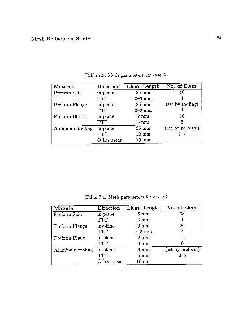
Mesh Refinement Study 64
Table 7.3: Mesh parameters for case A.
Material Direction Elem. Length No. of Elem.
Preform Skin in-plane 25 mm 10
TTT 2-3 mm 4
Preform Flange in-plane 25 mm (set by tooling)
TTT 2-3 mm 4
Preform Blade in-plane 2 mm 16TTT 3 mm 6
Aluminum tooling in-plane 25 mm (set by preform)
TTT 10 mm 2-4
Other areas 10 mm
Table 7.4: Mesh parameters for case C.
Material Direction Elem. Length No. of Elem.
Preform Skin in-plane 6 mm 38
TTT 3 mm 4
Preform Flange in-plane 6 mm 20
TTT 2-3 mm 4
Preform Blade in-plane 2 mm 16TTT 3 mm 6
Aluminum tooling in-plane 6 mm (set by preform)
TTT 6 mm 3-6
Other areas 10 mm

Mesh Refinement Study
7.8 Future Work
65
A full three-dimensional verification of these recommended element sizes should be con-
ducted. The results presented here should be used as a starting point in that study. Another
area that should be explored is where in the model the mesh refinement would do the most
good. This study used a uniform mesh in each direction. Refining the model near the
surface of the tools where the convective boundary condition is applied, or refining the
mesh near the tool/preform interface may provide better results than the uniform meshing
scheme currently used.
Chapter 8
Flow Model Verification
One of the most critical aspects of an RTM/RFI simulation program is accurate prediction
of the flow through the preform. Before a simulation program can be used, it must be
verified against experimental data. There are some questions that arise when verifying the
program. First, how accurate are the inputs to the model? Since preform permeabilities
are measured in a single direction at a time, how accurate is it to use these one-dimensional
permeabilities in three-dimensional tensor form as an input to the model? Second, given
accurate inputs, can the code adequately predict the three-dimensional flow pattern? To
answer these questions, a model was constructed to simulate the flow in a "T-stiffened"
section and the simulation results were compared against experimental results. This chapter
will discuss the three-dimensional flow experiment and the finite element simulation model,
and will compare the results obtained.
66
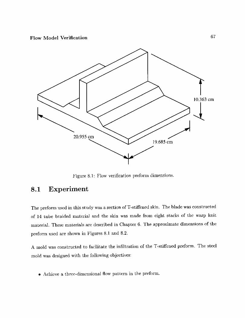
Flow Model Verification 67
20.955cm
19.685cm
10.363cm
Figure 8.1: Flow verification preform dimensions.
8.1 Experiment
The preform used in this study was a section of T-stiffened skin. The blade was constructed
of 14 tube braided material and the skin was made from eight stacks of the warp knit
material. These materials are described in Chapter 6. The approximate dimensions of the
preform used are shown in Figures 8.1 and 8.2.
A mold was constructed to facilitate the infiltration of the T-stiffened preform. The steel
mold was designed with the following objectives:
• Achieve a three-dimensional flow pattern in the preform.

Flow Model Verification 68
Z 1.118cm 0.853cm
10.363cm
t
-_---.--1.707 cm
3.224 cm
0.853 cm
-" 20 955cm "-
Figure 8.2: Flow verification preform dimensions.
• Compact the preform to 57% carbon fiber volume fraction.
• Provide a seal along the edges of the preform.
• Create boundary conditions that are easily modeled in the simulation code.
• Dimensionally stable during resin injection under elevated pressure.
The mold consists of four pieces, each constructed from steel. They are a base plate, a
picture frame, and left and right mold plates. The interior dimensions of the mold are fixed
to provide the correct compaction of the preform.
The mold has a single injection port located in the center of the base plate. The sides of
the mold are closed and the top of the stiffener is open to the atmosphere. Mounted in
the mold are 12 Entran EPX series pressure transducers. The locations of the transducers
in the mold are shown in Figure 8.3. The transducers were used to measure the passage

Flow Model Verification 69
1110 0
9 0 a0
12
0
Figure 8.3: Pressure transducer locations.
of the flow front, and to measure the fluid pressure inside the mold. The diameter of the
transducer is 3.5mm. The tip of the transducer was set back into the face of the mold so
it would not interfere with the flow front. Transducers 1-4 are located in the base plate,
along the center line. Transducers 5-7 are located on the top of the flange. Number 8 is
located on the skin, and 9-12 are located on the blade.
The pressure data from the transducers were recorded using LabVIEW software running
on a PC [28].
A Parker Hannifin Corp. Zenith constant flow rate pump was used to infiltrate the preform.
A flow rate of 3 cc/min was used. The fluid used was corn oil and the viscosity of the oil
was measured to be 0.054-0.057 Pa.s.
The mold was designed with the intent that it would provide an adequate seal around the
edges of the preform; but an initial run showed that the oil tended to leak around the edges.

Flow Model Verification 7O
All subsequent runs had the edges of the preform coated with vacuum grease to prevent
leakage.
8.2 Simulation Model
A three-dimensional finite element model of the preform was constructed. Three different
models were run using the isothermal, constant viscosity, flow-only option of 3DINFIL.
All three models used the same finite element mesh, but different numerical values for the
permeabilities and fiber volume fractions were input into each model.
8.2.1 Geometry and Boundary Conditions
The preform has two lines of symmetry, so only one-quarter of the preform was modeled.
A picture of the finite element mesh is shown in Figure 8.4. A total of 3496 elements and
4569 nodes were used to construct the model. The diameter of the inlet port was 1.111 cm.
Since the model was constructed with hexahedral elements, the inlet port was modeled as
a square having the same area as the circular inlet port.
There were two boundary conditions applied to the finite element model. The first is the
constant flow rate condition. To simulate the experimental flow rate of 3 cc/min a constant
flow rate of 0.75 cc/min was applied to the model. This flow rate is only one-fourth of the
experimental value because of the symmetry in the model. The second boundary condition
was the pressure sinks. These pressure sinks simulate the areas of the mold that were left
open to the atmosphere. Sinks were applied to the top of the blade and the outside corner
of the skin.

71
Flow Model VerificatiOn
_Z Inlet
Figure 8.4: Quarter symmetry finite dement mesh.

Flow Model Verification
y BladeMaterial
Fillet MaterialFlangeMaterialX
SkinMaterial
72
Inlet Material
Figure 8.5: Flow materials in the flow verification model.
Other inputs to the model include the viscosity of the oil and the permeability of the
preform. The viscosity used in the modeling was 0.055 Pa.s.
8.2.2 Permeability Calculation
The preform was divided into five regions and permeabilities were applied to each as shown
in Figure 8.5.
The fiber volume fractions for the skin and blade were calculated as follows. First, the
volume fractions were determined by using the areal weight of the preform Aw, the thickness
of the closed mold t, and the density of carbon fiber p::
Aw
v:=(8.1)
The parameters and the computed values of the fiber volume fractions are shown in Ta-
ble 8.1. Once the fiber volume fractions are known the permeabilities were computed using
the fit constants in Appendix B.

Flow Model Verification 73
Table 8.1: Calculatedfiber volumefractions of the T-section.
Aw (g/cm 2) t(cm) p_ (g/cm 3) vf
Skin 1.23 1.1176 1.8 0.61
Blade 1.80 1.7068 1.8 0.585
No compaction data were available for the region where the skin and flange are joined. For
this region it was assumed that the skin fiber volume fraction was 61%, the same as for
the rest of the skin. The flange fiber volume fraction was assumed to be 58.5%, the same
as the blade fiber volume fraction. To test the sensitivity of the model to changes in the
flange fiber volume fraction, the flange fiber volume fraction was run with both 58.5_ and
61%. Very little difference in the fill times and pressures was observed.
To investigate the role that permeability played on the predicted pressures and fill times,
three different models, designated as A, B, and C, were run. Table 8.2 summarizes the
fiber volume fractions and permeabilities used in each finite element model. No data were
available for the 14 tube braid, through-the-thickness permeability, so the permeability of
the 4 tube braid at the same fiber volume fraction was used. The 4 elements at the inlet
of the model were given a very high permeability of 1.0 x 10 .5 m 2 to minimize their effects
on the inlet pressures.
8.2.3 Mesh Convergence
The mesh shown in Figure 8.4 was determined to be converged for both the flow times and
the pressures at all 12 of the pressure taps.
The inlet area of the mesh was not converged. Three different local models of the inlet area
were run. One had 2x2 elements covering the inlet, one had 4x4, and one had 8x8. This

Flow Model Verification 74
Table 8.2: Three-dimensional flow model fiber volume fractions and permeabilities.
Permeabilities in m 2
Model Skin I Blade [ Flange Fillet
A vfIPP
IPN
TTT
B vyIPP
IPN
TTT
C vyIPP
IPN
TTT
0.61
3.72 x 10 -12
1.60 × 10 -12
6.41 x 10 -13
0.645
1.90 × 10 -12
8.00 × 10 -13
4.13 × 10 -13
0.645
1.90 × 10 -12
8.00 x 10 -13
4.13 × 10 -13
0.585
8.50 × 10 -12
5.43 × 10 -12
6.01 × 10 -13.
0.606
4.48 x 10 -12
2.71 × 10 -12
4.44 x 10 -13.
0.606
4.48 × 10 -12
2.71 × 10 -12
4.44 × 10 -13.
0.585
1.36 × 10 -11
4.88 × 10 -12
6.01 × 10 -13
0.606
7.77 x 10 -12
2.79 × 10 -12
4.44 x 10 -13
0.606
7.77 × 10 -12
2.79 × 10 -12
4.44 × 10 -13
(Use flange perms)1.36 × 10 -11
4.88 × 10 -12
6.01 × 10 -13
(Use flange perms)
7.77 × 10 -12
2.79 × 10 -12
4.44 × 10 -13
N/A
1.0 × 10 -10
1.0 x 10 -1°
1.0 × I0-1°
* No 14 tube TTT data available, computed using 4 tube TTT fit.
area of the model is difficult to model accurately for a number of reasons. First, 3DINFIL
only uses brick type elements which are good for modeling angular geometry, while the
inlet is round. Second, local models of the inlet area were very large and used up to 96
hours of CPU time on an SGI Origin machine. Even though the local models had not
converged, the model was predicting pressures of at least three to five times greater than
those measured in the experiment, and the pressure was rising with every mesh refinement.
It was determined that the fixture was probably leaking at the inlet port between the mold
surface and the bottom of the preform, so no further attempts to refine the inlet mesh were
made.
It was also found that changing the mesh size near the inlet had no effect on the calcu-
lated pressures or fill times at other locations in the model. Because the experiment was
conducted with a constant flow rate, the pressures near the inlet did not affect the rest of
the model for the mesh shown in Figure 8.4.

Flow Model Verification 75
8374.7816.
7258.6700.6141.5583.5025.4466.3908.3350.2791.2233.1675.1117.558.3
.0006104
Figure 8.6: Case A flow front progression. The color bands represent the flow front
location at different times. The units are in seconds.
8.3 Results
The predicted flow front locations for the three models are shown in Figures 8.6-8.8. Two
experimental runs were performed at 3 cc/min. Shown in Figures 8.9-8.13 are comparisons
between the measured pressures and the finite element model predicted pressures. Com-
parison of the predicted and measured infiltration times is shown in Figures 8.14 and 8.15.

Flow Model Verification 76
8093.7554.7014.6475.5935.5395.4856.4316.3777.3237.2698.2158.1619.1079.539.5
-.001953
Figure 8.7: Case B flow front progression. The color bands represent the flow front
location at different times. The units are in seconds.
Y
8918.8324.7729.7135.6540.5946.5351.4756.4162.3567.2973.2378.1784.1189.594.6
.001465
Figure 8.8: Case C flow front progression. The color bands represent the flow front
location at different times. The units are in seconds.

Flow Model Verification 77
90
8O
70
60c_
0_
5O
_ 40
0_
30
2O
10
I
0
Inlet PressureI I I I I
• t . -:'.--. _ ......................... :...... _ .......... : ...........
i / : 2.
/y. " ,...... i ............ i.............................................................
......................................I iiiii iiii!ii:iin::tt1 i I L
0 20 40 60 80 100 120 140Time (min)
Figure 8.9: Inlet pressures for different meshes.

Flow Model Verification 78
25
20
_15n
10-ICI)59
0_ 5
Pressure Port 1 & 4
01
! ! !
1A-------A Transducer #1 run2 _. i .,,a,_
- I '7-----_ Transducer ,4 run 2 ........... i...... __,_ .....I G_---e Transducer #1 run 3 i __._._----_-"_
- 1H Transducer #4 run 3 ......... _J_'_.allilil_lm'_.._ ' -i .........] - - - Model case A J__-' _Y"/ i
I ..... Model case B __-_ = .....
-5 i i i i i I
0 20 40 60 80 100 120 140Time (min)
ii20
t_{:L
"'15
,e13..
5
Pressure Port 2 & 3
01
-50
! ! ! !
_ A-----A Transducer #2 run 2 __Transducer #3 run 2
_ _ Transducer #2 run 3I,i i ......
H Transducer #3 run 3 ____- - - Model case A .... _._llilJ/_N.,...\ ....... :
Ib
..... ModelcaseB iliill_lBE__ :: . ..-_------
-- Model case C __. _i C ......... :
i I i l 1 (
20 40 60 80 100 120 140Time (min)
Figure 8.10: Comparison between the measured and model predicted pressures at ports
1 & 4 and 2 & 3. Pressure transducer locations are shown in Figure 8.3.
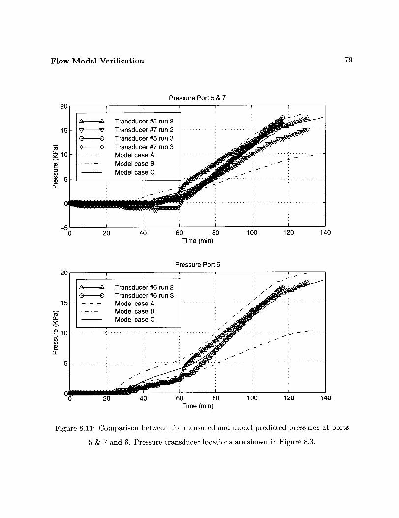
Flow Model Verification 79
20
15
Q.,,,, 10v
_ 5
01
Pressure Port 5 & 7
Transducer #5 run 2 ,_
-- _ Transducer #7 run 2 ........... i............ !/__' -Transducer #5 run 3 : .__'
H Transducer #7 run 3 i ..__" i
..... Model case A .......... _ _ C_ -- ""..... Model case B J,a_ _ i _ _ _
Model case C .Jr< ,7. _ ." .....................
-5 i i l i0 20 40 60 80 100 120 140
Time (Tin)
20
15
13-
v
-_10.-1
q}
C0
Pressure Port 6I I I .' ' ' /
Transducer #6 run 2 . X,,_ID,._a_ _j_
O--------O Transducer #6 run 3 /./__- - - - Model case A ........... i......... ./"_ .... i .........
..... Model case B : . " _ :
-- Model case C ' //_ ::
............. • ............ ,.......... , , . ,...,
, , , / . / ,
i i i /' 1./ i[ ] , ..- I , .• • •,I" . I , .
i / /_
i /" •
20 40 60 80 100 120 40Time (min)
Figure 8.11: Comparison between the measured and model predicted pressures at ports
5 & 7 and 6. Pressure transducer locations are shown in Figure 8.3.

Flow Model Verification 80
Pressure Port 8
7 _ _ _
6 " _ Transducer #8 run 2 ........... i ............ i ......... _ : " /_,Transducer #8 run 3 i i _ i /2&
5 .. --- ModelcaseA ........... :............ : ........ _:_ _"....
..... ModelcaseB i i .2. /i _.../
_ 4 .. ........... !............ ! ...... ij! "J-Model case C
3 ............. :............ i............. : ............ !............ ! .... _:_- l--....... : '_, .....
P_ 2 ............. i............ i............ i............ i............ i. _........
, .............::............i..................................... ...........c '" ! -- i i : _I _ :
-1 i i i0 20 40 60 80 100 120 140
Time (min)
15
Pressure Port 9 & 12
10
5
01
-5
Transducer #9 run 2
Transducer #12 run 2 .... ,,_i_..,_!___" _ Transducer #9 run 3 ......... : ' J
Transducer #12 run 3 ! ,4_"_,,.,_,,- - - Model case A : ,,_Y"d_#_ :..... Model case B .......... !__'.. _....,_.......
-'" _ ModelcaseC ,__,4_ :: _''_-
1
0 20 40 60 80 100 120 140Time (min)
Figure 8.12: Comparison between the measured and model predicted pressures at ports
8 & 9 and 12. Pressure transducer locations are shown in Figure 8.3.
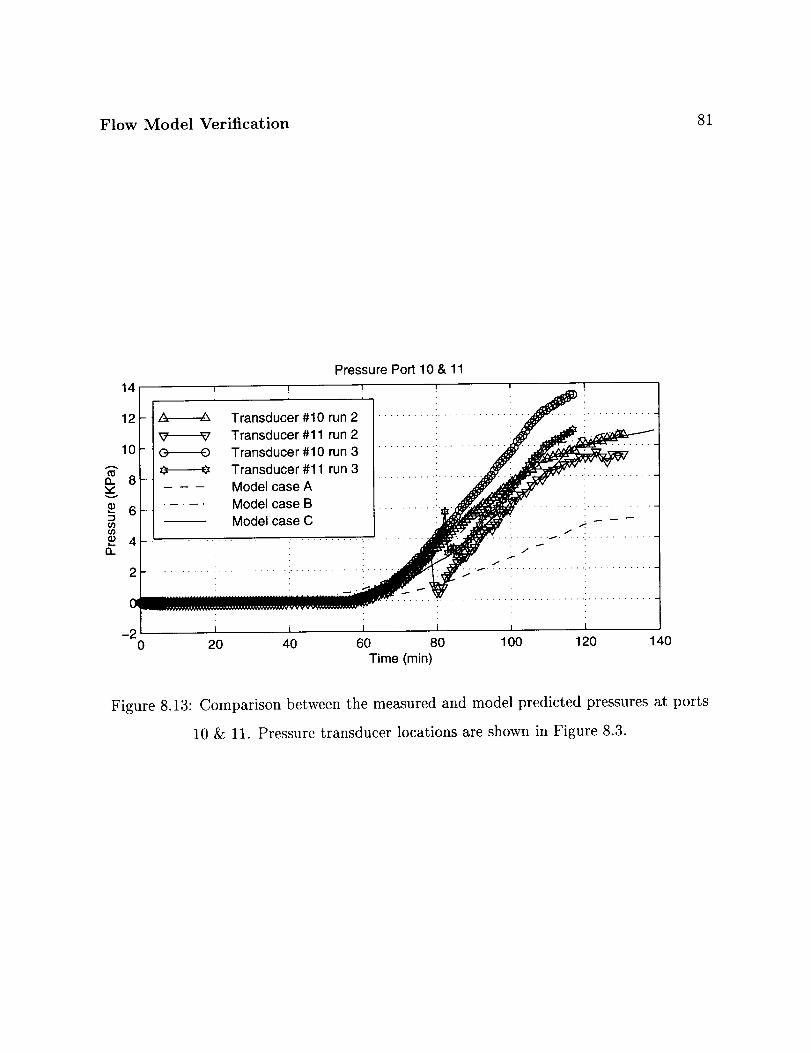
Flow Model Verification 81
14
12
10
a. 8v
6--I¢o¢o•_ 4
fl_
2
-20
Pressure Port 10 & 11I I I I
Transducer #10 run 2 .........................
Transducer #11 run 2 ...... ._Transducer #10 run 3 ......... i
... _ Transducer #11 run 3 .......... :....... _- - - Model case A : _',ad_
._.. .... Model case B ........... ,,, ,_i._.,d_,,,d_i_t;_.----,_._,_,_,......................_Model case C :_': ,; - -
....................... _ 'i........ _..: ...........
I i i i i i
20 40 60 80 1O0 120 140Time (min)
Figure 8.13: Comparison between the measured and model predicted pressures at ports
10 & 11. Pressure transducer locations are shown in Figure 8.3.

Flow Model Verification 82
O, LL
I.'L.
6"17
O
OJ
GO
CO
o_LO
COo_OJ
o_T"
0 0 0 0 0 0 0o d o o d o d0,.I 0 CO (.0 _
(u!tu) etU!l II!JUl
Figure 8.14: Experimental and predicted infiltration times for the flow verification model.

Flow Model Verification 83
oto04
I
mDm
sauJ!_ II!:1 jo
gouoJag!Q aEm, uaoJad
Figure 8.15: Percent difference of wet out times for the flow verification model.

Flow Model Verification
8.4 Discussion
84
8.4.1 Inlet Pressure
The measured and model A predicted pressures for the inlet pressures are shown in Fig-
ure 8.9 on page 77. The 4x4 and 8x8 cases were local models of the inlet, so they were only
valid for the first 34 minutes of the simulation. The model has obviously not converged, but
it can be seen that the pressures are increasing with each mesh refinement. The predicted
pressures are about three to four times higher than the measured pressures. The inlet is the
only port in case A where the model overpredicted the pressures. At all of the other ports
the model underpredicted the pressures. This suggests that the fluid may be compressing
the preform near the inlet and leaking between the skin and the baseplate. The infiltration
times shown in Figure 8.14 for ports 1&4 and 2&3 support the idea that there is a leak
path near the inlet. All three simulation models overpredict the infiltration time of these
ports.
The leak path probably exists because the area under the blade is not supported on both
sides by the mold and no direct compaction of that area is available.
8.4.2 Skin, Flange, and Blade Pressures
The pressure curves predicted by case A show the same general shape as the experimental
curves, but they seem to be too low by a factor of two. One input that may be causing
this mismatch is incorrect permeabilities being used in the model. The permeabilities of
the materials were calculated from only two or three samples, and all of these samples
came from the same batch of materials. The preforms were constructed from a different
batch, and the batch-to-batch variability of these materials is unknown. Another factor

Flow Model Verification 85
that would affect the permeability is the actual arealweight of the preform. Again, there
is no data on the batch-to-batch variability of this quantity.
To attempt to match the pressures, the in-plane permeabilities would have to be reduced
by a factor of two. One method to vary the permeabilities would have been to individually
vary each principal permeability and check its effect on the pressures. This did not seem
appropriate because the three principal permeabilities are not independent of each other,
but they all depend on the fiber volume fraction of the preform. Therefore, to affect this
change in the permeabilities, it was decided to find a fiber volume fraction that would result
in a reduction of the in-plane permeabilities by a factor of two. The fiber volume fractions
found were 64.5% for the skin and 60.6% for the blade. The permeabilities calculated from
these fiber volume fractions are listed in Table 8.2 on page 74. The model run designated
as case B used these permeabilities.
On comparing the flow front shapes of case A (Figure 8.6) and case B (Figure 8.7), there
is no significant change in the shape of the front. The calculated pressures from case B
match the experimental curves well.
Details of case C will be discussed in the next section, but it should be noted that the
predicted pressures of case C also match the experimental curves well.
8.4.3 Fill Times
Once the pressures had been matched, an effort was made to more precisely model the
preform. In cases A and B, the unidirectional fibers in the fillet region were not taken into
account, and the elements in those models were given the same permeability as the flange
region. Case C attempted to model the fillet region more accurately. The fillet region was
given a higher permeability of 1 x 10 -1° m 2. Inspecting the flow front shape of case C in

Flow Model Verification 86
Figure 8.8 showsthat the fluid tends to prefer to flow along the fillet regionbefore it fills
the rest of the preform. After the flow fills the area around the inlet, it becomesmostly
planar as it flowsup the blade and acrossthe skin.
Figures8.14and 8.15showgraphscomparingthe predictedand measuredinfiltration times.
Model caseC agreeswith the experimentto within about +10%.

Chapter 9
Stepped Panel Simulation
A three-dimensional model was used to simulate the resin film infusion processing of a
stepped textile preform.
9.1 Experiment
9.1.1 Preform and Tooling
The textile preform used in this experiment was constructed from stacks of the warp knit
fabric described in Chapter 6. Figure 9.1 is a sketch of the preform. Each step is two stacks
thick. The thinnest part of the preform is two stacks thick and the thickest is eight stacks.
After stitching, eight stacks are approximately 1 cm thick. The preform weighed 1961 g
(1520 g/m2/stack).
Figure 9.2 shows a sketch of the tooling used to process the panel. Both the base plate and
the top plate were constructed from 6061-T6 aluminum. The base plate was approximately
1.27 cm x 76.2 cm x 152.4 cm. The top plate was 25.4 cm wide and 101.6 cm long and
87
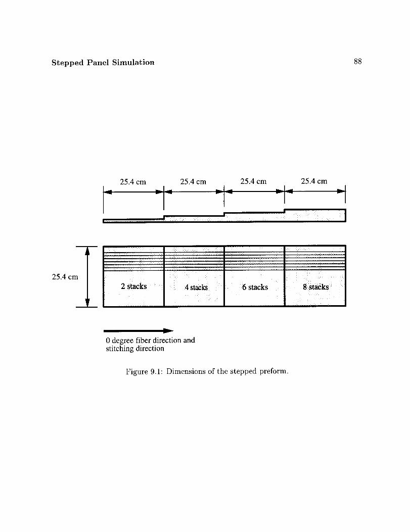
Stepped Panel Simulation 88
25.4cmI_...
25.4cm 25.4cm 25.4cm.._1-.. ..._I_.. ..._1_... ..._1
I I
25.4 c
I I '2 stacks • 4 stacks 6 stacks 8 stacks
=
y
0 degree fiber direction andstitching direction
Figure 9.1" Dimensions of the stepped preform.

Stepped Panel Simulation
Top PlateSecondarySeal
BleederCloth -- VacuumBag
89
PrimarySeal ResinFilmPreform BasePlate
Figure 9.2: Tooling and layup of the steppedpanel.
its thicknessrangedfrom 1.590cm to 2.413cm. Detailed drawingsof the top and bottom
plates can be found in Appendix A.
9.1.2 Procedure
First, the top and bottom plates were instrumented with thermocouples, Dek Dyne fre-
quency dependent electromagnetic sensors (FDEMS), and Entran pressure transducers,
model EPX0-X03-150P with a 7.6 mm tip. The thermocouple, FDEMS, and transducer
locations are shown in Figures 9.3-9.5, respectively. Thermocouples 1-4 were located be-
tween the preform and the top mold, 5-7 were located between the baseplate and the resin,
and 8-12 were located in the autoclave air. Thermocouples 8-12 had their leads taped to
the part, and the leads were bent so the head was about 5 centimeters away from the part.
Thermocouple 3 failed during the experiment.
The pressure transducers were recessed into the tooling to minimize their effects on the

Stepped Panel Simulation
_mTC5 _C 7
TC 8,12m] __C 10,11 "m[[m
TC 4 TC 2 TC 1
+5.1 cm
1-10.2 cm
9O
12.7 cm 12.7 cm 12.7 cm 12.7 cm
_¢I'C 10 "[]'q'C 9 _1'¢I'C 8
+12.7 cm
1
4'¢I'C 11 _]_l'C 12
Figure 9.3: Locations of the thermocouples on the stepped preform.
flow front.
A FDEMS consists of a fine array of two interdigitated comb electrodes. These sensors can
be used to monitor in situ the processing properties of thermoset resins. The FDEMS is
able to monitor the progress of cure, viscosity, and buildup in modulus. The data obtained
from the sensors in this experiment was used to detect the passage of the flow front. Details
regarding the sensor measurements are described in [31].
This experiment used the reduced catalyst 3501-6 resin. The resin was degassed at 85°C
for 25 minutes in a vacuum oven. The degassing process formed 25.4 cm x 25.4 cm resin
tiles. Each tile was approximately 0.6 cm thick and the total resin weight was 1208 g. The
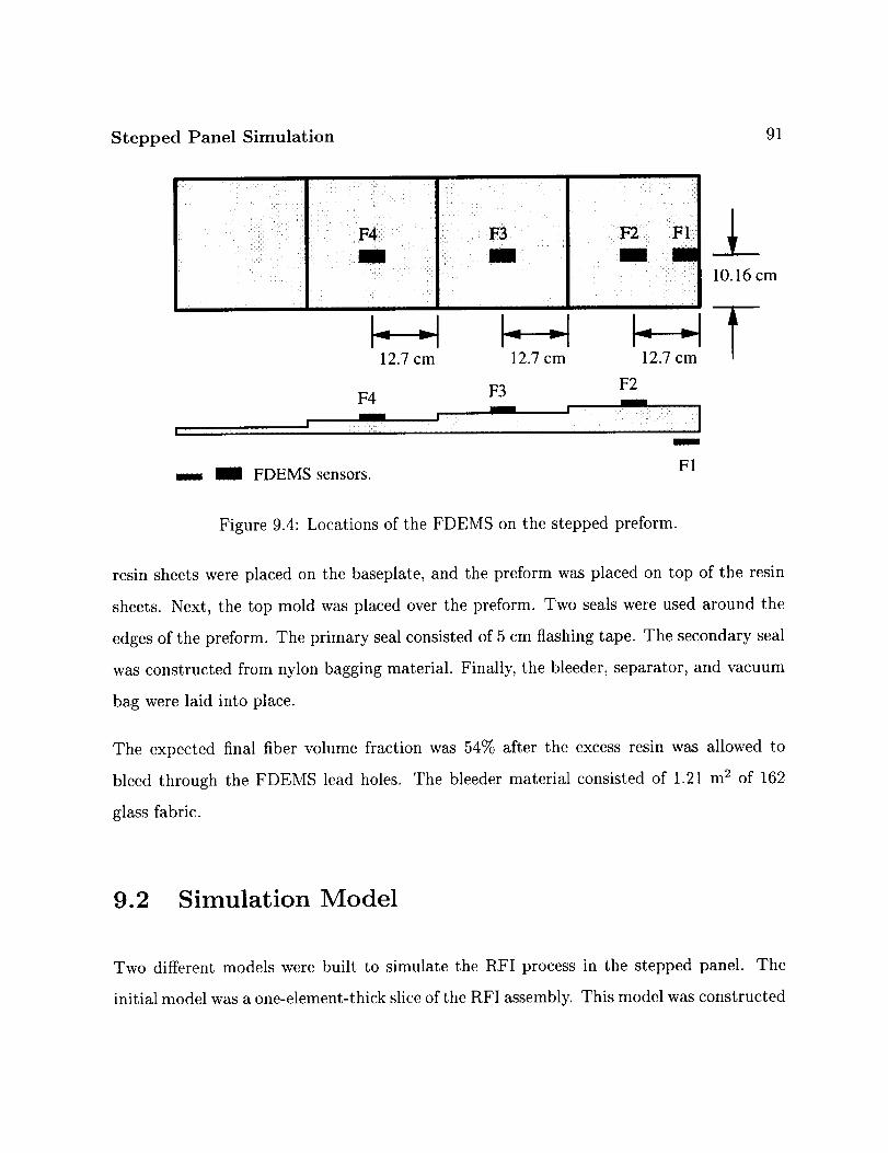
Stepped Panel Simulation 91
!
F4
12.7 cm 12.7 cm 12.7 cm
F3 F2
10.16 cm
_ FDEMS sensors.
Figure 9.4: Locations of the FDEMS on the stepped preform.
resin sheets were placed on the baseplate, and the preform was placed on top of the resin
sheets. Next, the top mold was placed over the preform. Two seals were used around the
edges of the preform. The primary seal consisted of 5 cm flashing tape. The secondary seal
was constructed from nylon bagging material. Finally, the bleeder, separator, and vacuum
bag were laid into place.
The expected final fiber volume fraction was 54% after the excess resin was allowed to
bleed through the FDEMS lead holes. The bleeder material consisted of 1.21 m 2 of 162
glass fabric.
9.2 Simulation Model
Two different models were built to simulate the RFI process in the stepped panel. The
initial model was a one-element-thick slice of the RFI assembly. This model was constructed

Stepped Panel Simulation 92
10.16cm 10.16cm 10.16cm 10.16cm
P2 P1P4 P3
l , l , I , lI
I P5 I P6 I P7
| ,ii
12.70 cm 12.70 cm
O Transducers mounted in the top mold.
t_ Transducers mounted in the bottom plate.
Figure 9.5: Locations of the pressure transducers on the stepped preform.
Stepped Panel Simulation 93
becauseit would run quickly and give initial estimatesof the fill times, temperatures,heat
transfer coefficients,and meshrequirementsto model this experiment. The final model
wasa full three-dimensionalmodel. From this model the full three-dimensionalflow field
wasfound, and the fill times weredetermined.
9.2.1 Model Geometry
The expected thickness of the preform was 1.37 mm per stack, or 2.74 mm per step. The
actual top plate was machined to these step heights. To try and more accurately model
the experiment, the thickness of each step of the preform was modeled using the cured
thickness of the panel. The measured thicknesses of each step were: 2 stack, 3.18 mm;
4 stack, 5.89 mm; 6 stack, 8.38 mm; and 8 stack, 11.02 mm. Because the actual thickness
of each step was not the same as the expected thickness, the model of the top plate had
to be adjusted. The model of the top plate was dimensioned to fit against the top of the
preform model by adjusting the step heights of the top plate model. The thin end of the
top plate was modeled as 15.90 mm thick, while the thick end was modeled as 23.75 mm
thick.
One reason the actual thicknesses of the steps were not the expected values was due to
the presence of resin rich areas at the bottom of the cured panel. This resin did not fully
infiltrate the preform, but "puddled" on the bottom of the panel. Another reason could
have been that the preform did not compact uniformly, and the top plate compacted the 8
stack step more than the 2 stack step.
Figure 9.6 shows a sketch illustrating the mesh used for the initial model. This model
is one element thick in the Z-direction. Each step has eight elements in the in-plane (X)
direction, and 2 elements in the through-the-thickness (¥) direction. The top plate had 14
elements on the left most step, and drops off two elements per step to 8 elements on the

Stepped Panel Simulation 94
14 elements
2 elem. 4 elem.
2 elements .....
per step
8 elements
Y
I-" 8 elements
per step
6 elem. 8 elem.
Figure 9.6: Initial one-element-thick finite element model.
right step. The baseplate had 8 elements through the thickness and 32 along its length.
A picture of the final model is shown in Figure 9.7. Only half of the actual preform/tooling
assembly was modeled due to the plane of symmetry down the middle. The final model
included the large baseplate used in processing. The baseplate extends approximately 25
cm to each side of the preform. The mesh for the final model is very similar to the initial
model. In the final model, the elements are smaller near the edges of the preform that are
in contact with the autoclave air. This was done because high thermal gradients had been
observed in the initial model near these areas.
A summary of the finite element meshes and run times for each model is shown in Table 9.1.
Both models were run on an SGI Origin system.

Stepped Panel Simulation 95
Figure 9.7: Final three-dimensionalfinite elementmodel.
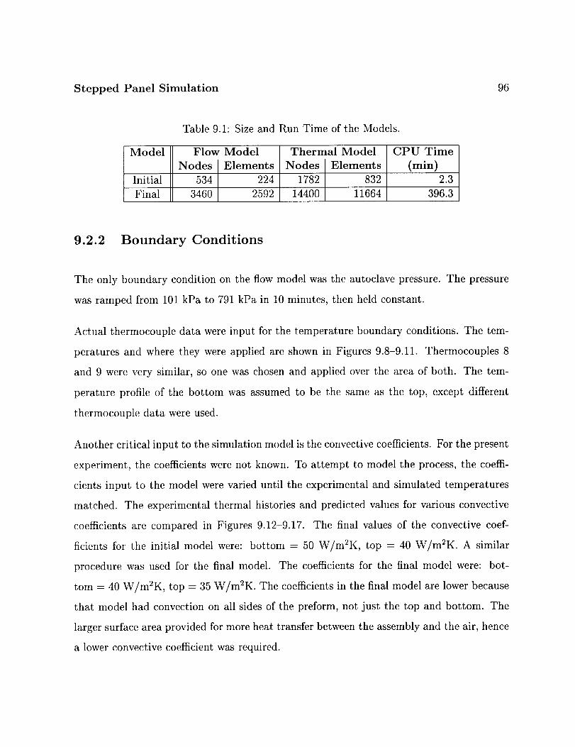
Stepped Panel Simulation 96
Table 9.1: Sizeand Run Time of the Models.
Model Flow Model Thermal Model CPU Time
Nodes Elements Nodes Elements (min)
Initial 534 224 1782 832 2.3
Final 3460 2592 14400 11664 396.3
9.2.2 Boundary Conditions
The only boundary condition on the flow model was the autoclave pressure. The pressure
was ramped from 101 kPa to 791 kPa in 10 minutes, then held constant.
Actual thermocouple data were input for the temperature boundary conditions. The tem-
peratures and where they were applied are shown in Figures 9.8-9.11. Thermocouples 8
and 9 were very similar, so one was chosen and applied over the area of both. The tem-
perature profile of the bottom was assumed to be the same as the top, except different
thermocouple data were used.
Another critical input to the simulation model is the convective coefficients. For the present
experiment, the coefficients were not known. To attempt to model the process, the coeffi-
cients input to the model were varied until the experimental and simulated temperatures
matched. The experimental thermal histories and predicted values for various convective
coefficients are compared in Figures 9.12-9.17. The final values of the convective coef-
ficients for the initial model were: bottom -- 50 W/m2K, top = 40 W/m2K. A similar
procedure was used for the final model. The coefficients for the final model were: bot-
tom = 40 W/m2K, top = 35 W/m2K. The coefficients in the final model are lower because
that model had convection on all sides of the preform, not just the top and bottom. The
larger surface area provided for more heat transfer between the assembly and the air, hence
a lower convective coefficient was required.
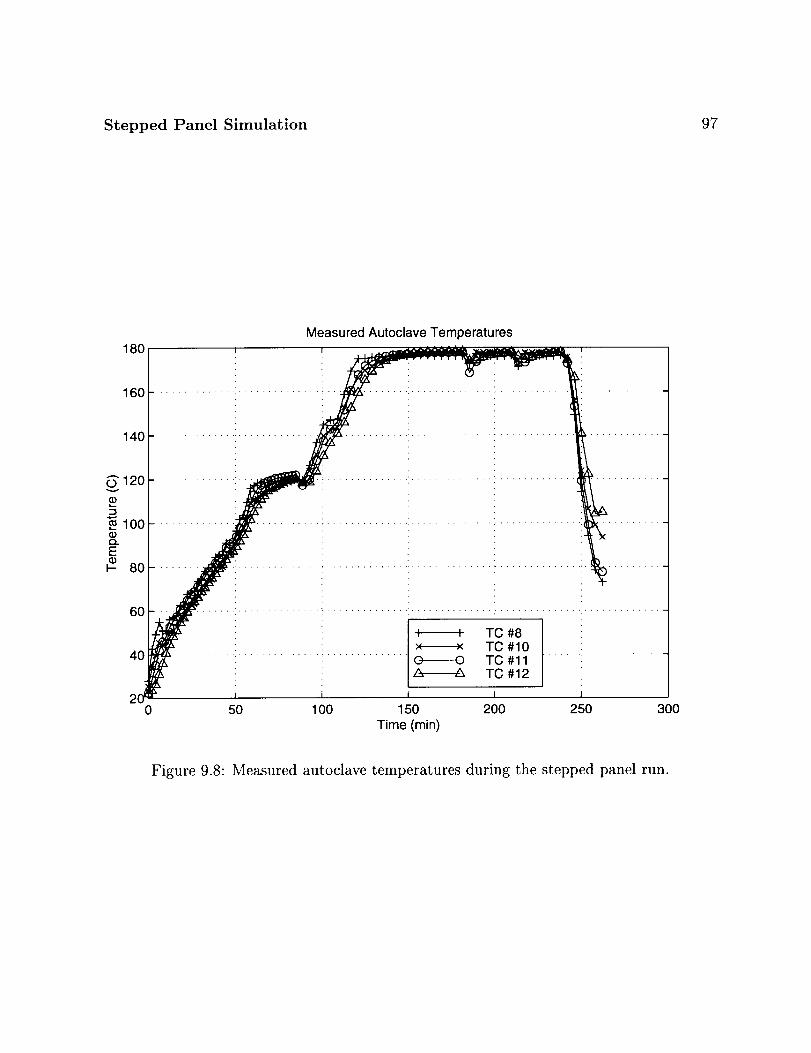
Stepped Panel Simulation 97
Measured Autoclave Temperatures180 ,
160 ...................... :............
140 ...........................
_" 120 ...........................................................v
100o_E
_- 80
6O
4O
0
TC #8TC #10TC #11TC #12
i I
50 100 150 200 250 300Time (min)
Figure 9.8: Measured autoclave temperatures during the stepped panel run.

Stepped Panel Simulation 98
Top Convective Coefficinet
Temp = TC # 10
_ I .,,,mill
Temp = TC #8
v
v
_1...
Temp = TC #11 Temp = TC # 12
v
Bottom Convective Coefficient
Figure 9.9: Applied temperature cycles for the initial model.
#8
Figure 9.10: Applied temperature cycles to the top of the final stepped model.

Stepped Panel Simulation 99
Y
Figure 9.11: Applied temperature cycles to the bottom of the final stepped model.
All error estimates were calculated against the total temperature variation of the applied
temperature cycle. The variation was 177°C - 25°C = 152°C, and Equation (9.1) was used
to calculate the error.
(predicted temp) - (experimental temperature)100%× (9.1)
177- 25

Stepped Panel Simulation 100
120
100
0v 80Q.E
t.-60
40
200
Temperature at point 1i I [ I I I
•..'''''"
. , j
.'" ,''" "'_
.." _ •
' I I I I I I
10 20 30 40 50 60Time (min)
I I I
;<_
x x TC#1
Model results:
.... top=25, bot=25
....... top=50, bot=50
top=40, bot=50
I I I I
70 80 90 100
Q}
o_
4
2
0
-2
-4
-6
-8
-100
\
\
\
Error between measured and calculated temperatures at point 1I I I i I I I i I
• , , . , . . . , , • , , • ,' , . , , , , , "''', ,,"
m
4 m
4
_ m
b
\
\
•,-.. ,
j n n n i I i .... "i" n
10 20 30 40 50 60 70 80 90Time (min)
J
100
Figure 9.12: Temperature profiles at thermocouple location 1 for various convective
coefficients. Thermocouple locations are shown in Figure 9.3.

Stepped Panel Simulation 101
120
100
o80
t_
E
60
40
20:0
Temperature at point 2I I I I I I I I I
• , • . • . . ."
• , * , • , j
....... top=50, bot=50
top=40, bot=50
.' .' j'
10 20 30 40 50 60Time (min)
I I I
70 80 90 100
5
0
-5
Error between measured and calculated temperatures at point 2I I I I I I I I I
• • , , ..... , , . . . ........
• . . . . . , . , . . , . • . , .'" • . . . . .
\
-1C I , , ,0 10 20 30 40
i
f_J
"_'. j
"%.. ,J
I I I I I
50 60 70 80 90 100
Time (min)
Figure 9.13: Temperature profiles at thermocouple location 2 for various convective
coefficients. Thermocouple locations are shown in Figure 9.3.

Stepped Panel Simulation 102
120
100
ov 80{3.E
1-
60
40
200
Temperature at point 4I i i I I I I I I
.... .......x.
.-._ x x TC # 4
.'S 1"' J Model results:
._x" _./ •-. - top=25, bot=25i
_xX.> ' _ •...... top=50, bot=50
_x.X _ -- top=40, bot=50
i
, , , T--C 710 20 30 40 50 60 70 80 90 100
Time (min)
6Error between measured and calculated temperatures at point 4
I I I i I I i I i
4
0
_-2
-4
-6
• • . • . , . + . . , ..... , , , . . .• . . , .... . + .
• . . . . . . • . . . .' •
• .., • ."
"%..
-8 i i i i i _ -- 10 10 20 30 40 50 60 70 80 100
Time (min)
'_.. i
I"
I l I
9O
Figure 9.14: Temperature profiles at thermocouple location 4 for various convective
coefficients. Thermocouple locations are shown in Figure 9.3.

Stepped Panel Simulation 103
120
100
o"-- 80Q.E(D
1--
60
40
200
Temperature at point 5I I I I I I
.' ..'''''
..'" f
.'" f.7
f f.f f
f '
f '
f "J
I I I I I I
10 20 30 40 50 60Time (min)
I I I
• . , . , ."
xX^t...I""
._ x_ /.1 ''_"
TC#5
Model results:
top=25, bot=25
top=50, bot=50
top=40, bot=50
× x
I I I
70 80 90 00
0
$-2
-4
-6
Error between measured and calculated temperatures at point 5I I I I I I I I I
..
\
\
\
• /\
• ._. /
I I I
/
".,_.../ -7
--8 I I I I I I
0 10 20 30 40 50 60 70 80 90 100Time (min)
Figure 9.15: Temperature profiles at thermocouple location 5 for various convective
coefficients. Thermocouple locations are shown in Figure 9.3.

Stepped Panel Simulation 104
120
100
{O"-" 80Q..E(D
I---
60
40
200
Temperature at point 6I I I I i I
10 20 30 40 50 60Time (min)
I I I
x x TC#6
Model results:
top=25, bot=25
top=50, bot=50
top=40, bot=50
I I i
70 80 90 100
2
0
-2
-4
-6
-8
. _ . . , . . . , , . . t
Error between measured and calculated temperatures at point 6I ] I I I I I I
\
\ • I
• /,%
k
\
\
k
\ f
\ i
-10 , , , , , I , , ,0 10 20 30 40 50 60 70 80 90 1O0
Time (min)
Figure 9.16: Temperature profiles at thermocouple location 6 for various convective
coefficients. Thermocouple locations are shown in Figure 9.3.

Stepped Panel Simulation 105
120
100
Ov 80
EF--
6O
40
I I I
Temperature at point 7I I I
xxX XXX
Xy e..1't'f
x x TC#7
Model results:
.... top--25, bot=25
....... top=50, bot--50
top=40, bot=50
xx
x x
x Xx x
xX_,, ,_ ..i'
xXZ .i 'I
xX_ , .--"
X X _._j,- , ..., , I
X ' "'/"/
_'/1" I I I I
X t't"
10 20 30 40 50 60Time (min)
2O: I I I
0 70 80 90 100
Q_
o_
0
-2
_z
-(
-8
-10
Error between measured and calculated temperatures at point 7I i l I i i I i .
_\ ..''" '..
." .'"
\
\
\
\
\
\
\
\
/
/
/
/
/
/
\
\ J
-I_" I i i i i i _ Jl' I I
0 10 20 30 40 50 60 70 80 90 1O0
Time (min)
Figure 9.17: Temperature profiles at thermocouple location 7 for various convective
coefficients. Thermoeouple locations are shown in Figure 9.3.

Stepped Panel Simulation
9.3 Results
106
Figures 9.18-9.23 show the predicted and measured temperatures at six locations on the
preform. Thermal errors were calculated as stated in Equation (9.1) on page 99. Figure 9.24
shows the predicted and measured wet out times for each step.
9.4 Discussion
9.4.1 Temperatures
Temperature results compare favorably between the model and the experiment. During
the infiltration of the preform (before 50 minutes) the predicted temperatures are within
3-4_ of the measured temperatures. There are a few interesting points to note. If you
look at the temperatures from the start of the experiment to about 20 minutes, the model
is seen to overpredict at every point. This is caused by the presence of the bleeder cloth in
the experiment. The bleeder will act like a blanket and slow the initial penetration of the
autoclave heat into the part. The thermal effects of the bleeder were not included in the
model, so the model begins to see the autoclave temperatures sooner than the real part.
After the initial lag time, the experimental and predicted temperatures begin to converge.
The highest error is found at thermocouple location 5 (see Figure 9.21). Both models show
a significant thermal overshoot as compared to the experiment. Point 5 is under the two
stack step, the thinnest step. As was noted in Chapter 7, this thermal overshoot is usually
caused by a mesh that is too coarse. This is very likely here, as this step is modeled by
only two elements through its thickness. If a finer mesh had been used in this step, the
thermal overshoot would likely be either smaller or non-existent.

Stepped Panel Simulation 107
200Temperature at point 1
I i
180
160
140
120Q..E
1001-
8O
60
40
200
x_ xxX
j Initial Model
/ F_inalModelI I I I
50 1O0 150 200Time (min)
25O
0
s_-1
-2
-3
-4
-50
Error between measured and calculated temperatures at point 1I I i I
! \
I I I I
50 1O0 150 200 250Time (min)
Figure 9.18: Comparison of thermal profiles at point 1. Thermocouple locations are
shown in Figure 9.3.

Stepped Panel Simulation 108
200
180
160
140
.....O120o..E
1001-
80
60
40
20
Temperature at point 2I I I I
.#
x TC#2
Initial Model
Final Modelj [
I I I I
0 50 100 150 200 250Time (min)
4
3
2
1
0
-1
-2
-30
Error between measured and calculated temperatures at point 2i I i I
!_\\ /\
_\ ._ i"/ \
X \-,'/ \ I \ f "" -- "fP
X\ i / \ \ ,,- ." ,/
vI I I 1
50 100 150 200Time (min)
250
Figure 9.19: Comparison of thermal profiles at point 2. Thermocouple locations are
shown in Figure 9.3.

Stepped Panel Simulation 109
200
180
160
140
o 12o¢._
E100
1-
80
60
40
2C0
Temperature at point 4I I I I
/'<
x TC#4
" Initial Model
Final ModelI I I I
50 1O0 150 200 250Time (min)
4
-1
Error between measured and calculated temperatures at point 4I I I i
/ \
\
•-. / \
\ // \
\ // \_./_\
\ I
--2 I I I I
0 50 1O0 150 200 250Time (min)
Figure 9.20: Comparison of thermal profiles at point 4. Thermocouple locations are
shown in Figure 9.3.

Stepped Panel Simulation 110
200Temperature at point 5
I I I I
180
160
140
o 120Q.E
100t--
8O
60
40
20"0
X--XX'-Xxxx_ x'-xx-xxxx x_xxXXX
v^..Xfxx
jxxj xx x x TC # 5
z,o¢"
" Initial Model
/ _ i , final Model
50 100 150 200Time (min)
25O
9
_5_)
o_4
3
2
1
00
Error between measured and calculated temperatures at point 5I I I I
/"\
/ \
! \
/ \
\\\\ -_
\ f ""
\ /
I I I I
50 100 150 200Time (min)
250
Figure 9.21: Comparison of thermal profiles at point 5. Thermocouple locations are
shown in Figure 9.3.

Stepped Panel Simulation 111
20O
180
160
140
Ov 120Q..E
100t--
80
60
4O
200
Temperature at point 6I I I 1
x"x_-x R-xk-xk-×R-xx-x x
J x x TC#6
" Initial Model
/ Final Model__" I I I /
50 100 150 200Time (min)
250
3
2.5
2
1.5
1
0.5
0\
N-0.5
-10
Error between measured and calculated temperatures at point 6I I
,I k I"
-I _ . ii . /f... k
•._ f/ \ -, / _ /( \ / \ / ,_/
l \.,, -..-/
/
//
I I I I
50 100 150 200 250Time (min)
Figure 9.22: Comparison of thermal profiles at point 6. Thermocouple locations are
shown in Figure 9.3.

Stepped Panel Simulation 112
200
180
160
140
0.0120
E100
1-
8O
60
4o !l
20 s0
Temperature at point 7
x x
#
TC#7
Initial Model
Final Model
I I I I
50 100 150 200
Time (min)250
o_
2
1
0
-1
-2
-3
-4
-50
Error between measured and calculated temperatures at point 7J J J J
A.
I \
I
I \
I
1\ I \\
_f \ J
\
/
/
/
/
/
/
/
/
/
I I I I
50 1O0 150 200 250Time (min)
Figure 9.23: Comparison of thermal profiles at point 7. Thermocouple locations are
shown in Figure 9.3.
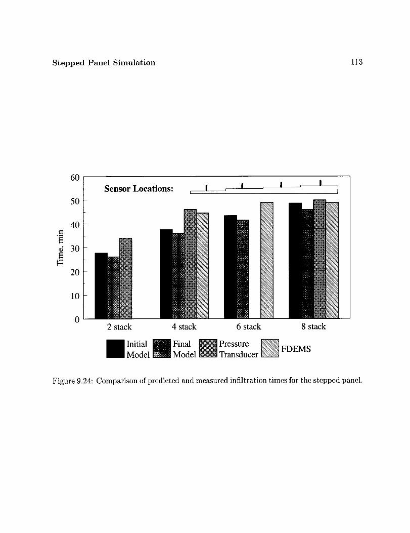
Stepped Panel Simulation 113
dE
60
50
40
30
20
10
0
Sensor Locations: I I , I , I, ' l
2 stack 4 stack 6 stack 8 stack
Initial l Final N Pressure _ FDEMSModel Model Transducer
Figure 9.24: Comparison of predicted and measured infiltration times for the stepped panel.

Stepped Panel Simulation
9.4.2 Fill Times
114
Fill times do not agree as well as the temperatures did. The model predicts earlier wet
out than the experiment for all the steps. The percentage difference between the predicted
and measured fill times are: 2 stack, -23%; 4 stack, -22%; 6 stack, -15%; 8 stack, -9%.
The general trend here is that as the steps get thicker, the difference between the predicted
and measured wet out times decreases. One explanation for this is that the filling of the
thin steps is dominated by flow at low temperatures. The kinetics model is based on data
at temperatures greater than 60°C, and viscosities for temperatures lower than that are
extrapolated from the viscosity model. The 2 and 4 stack sections fill while the highest
temperature in the model is about 50°C. This indicates that the viscosity model tends to
underpredict the viscosity for low temperatures.
The measured wet out times for the 6 and 8 stack steps were identical. This seems to
indicate that after the 4 stack step was filled, the resin may have leaked between the top
tooling plate and the preform, resulting in early wet out times for the 6 and 8 stack steps.
9.5 Conclusions
Given the correct heat transfer coefficients, the model is able to match the measured tem-
peratures in the experiment. Finding these convective coefficients will be necessary before
the model can be used in predictive work.
The fill times matched better for the thicker sections than the thinner sections. This was
probably due to the inaccuracy of the viscosity model below 60°C. As the flow through the
preform was dominated by flow at warmer temperatures, the viscosity model moved into
the range of temperatures it was based on, and the viscosity results were more accurate.

Chapter 10
Two Stiffener Panel
A panel with two stiffeners was manufactured using the RFI process. A two stiffener panel
was chosen because the complex shape will introduce a three-dimensional flow pattern.
The process was simulated using 3DINFIL and the simulation results are compared to the
experimental results. The objective of the test was to verify the flow, cure, and thermal
models in a complex shaped RFI part.
10.1 Experiment
10.1.1 Preform and Tooling
The preform skin was constructed of eight stacks of the warp knit fabric and the blades
were constructed from the 14 tube braided material described in Chapter 6. Sketches of
the preform are shown in Figure 7.2 on page 46 and Figure 10.1.
The mold for this part was constructed from 6061-T6 aluminum. A sketch of the tooling
is shown in Figure 10.2. The base plate was approximately 121.92 cm long by 60.96 cm
115

Two Stiffener Panel 116
10.31cm
45.87cm60.96cm
Figure 10.1: Sketchof the two stiffener preform.
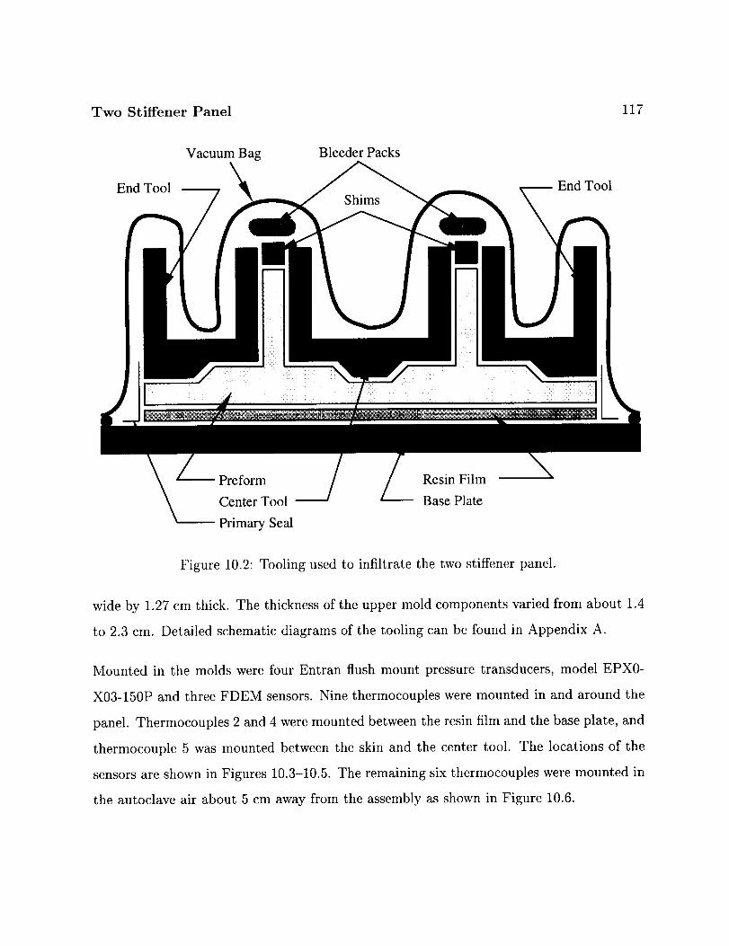
Two Stiffener Panel 117
EndTool
VacuumBag BleederPacks
ShimsTool
Preform ResinFilm
CenterTool BasePlate
PrimarySeal
Figure 10.2: Tooling usedto infiltrate the two stiffener panel.
wide by 1.27cm thick. The thicknessof the upper mold components varied from about 1.4
to 2.3 cm. Detailed schematic diagrams of the tooling can be found in Appendix A.
Mounted in the molds were four Entran flush mount pressure transducers, model EPX0-
X03-150P and three FDEM sensors. Nine thermocouples were mounted in and around the
panel. Thermocouples 2 and 4 were mounted between the resin film and the base plate, and
thermocouple 5 was mounted between the skin and the center tool. The locations of the
sensors are shown in Figures 10.3-10.5. The remaining six thermocouples were mounted in
the autoclave air about 5 cm away from the assembly as shown in Figure 10.6.

Two Stiffener Panel 118
5.08 cm 2.54 crl
i
i1
jr.. ,,i_ilm_mmJ_ lW,
. .
li i .
| i
F|
t
I
i
II
nlt_ I . I I .
• |
I I I , n l, - n I !
| •
| I
F2
F1
F5
FDEM sensors
Figure 10.3: Locations of the FDEM sensors on the two stiffener panel.

Two Stiffener Panel 119
i! !¸_¸
5.08 cm 2.54 crr
ii_!ilI ii_
! I i :
i .... I I| a
• I| : ]
i.... i : :
|
.... , I ] I, ]• I | I
i il '"
• I I ! , ..............
_i_iiI_i_ -,i
I ¸ I _ii !!i!i ¸¸¸¸_' ............_ if: it ¸;!i,i_iil /_i ¸
, I : i iI |
: I l, ,,,,, ,:
i P4
P|
P2 II
/_iil il _i _ _ : _ _JL _
m P3
i_ !ii!,i__,'i ij_ii_ii_ii_ii_i_ilI _il
Pressure transducers
Figure 10.4: Locations of the pressure transducers on the two stiffener panel.

Two Stiffener Panel 120
:! In n I i
I', !i
:!i ill ¸ :i!i!i /i_ L ¸ i ¸"
5i08cm: :2'54cn
I I ::: i I I
r i! !!a
I I
' |
= •
TC 5
/ "x_.+__/ \I I
TC 2,4
.4= Thermocouples
Figure 10.5: Locations of the thermocouples on the two stiffener panel.
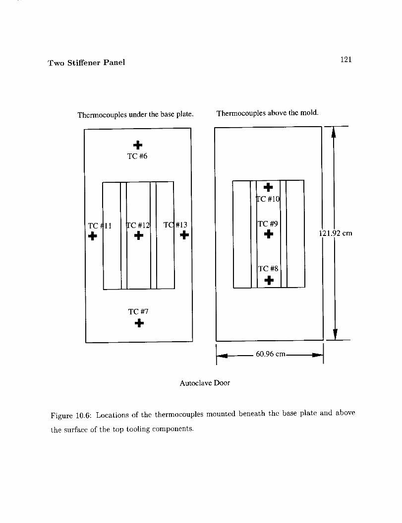
Two Stiffener Panel 121
Thermocouplesunderthebaseplate.
4"TC #6
TC :_11 FC #1_
4" 4,
I!
!
TC #7
4,
Thermocouples above the mold.
4,FC #10
TC #9
÷
TC #8
121.92 cm
60.96 cm v
Autoclave Door
Figure 10.6: Locations of the thermocouples mounted beneath the base plate and above
the surface of the top tooling components.

Two Stiffener Panel 122
Table 10.1: Sizeand Run Time of the Models.
Model Flow Model Thermal Model CPU TimeNodes Elements Nodes Elements
Initial 1008 434 2112 970 3.8 minFinal 8995 7276 17325 14994 77.8 hr
10.1.2 Procedure
The panel was laid up following the same procedure as the stepped panel in Chapter 9.
10.2 Simulation Model
Following the same procedure used for the stepped panel, two models were built of the two
stiffener panel. The initial model was one element thick in the Z-direction, and the final
model was a fully three-dimensional model.
10.2.1 Geometry and Mesh
The dimensions of the model were defined by the tools. The only dimension not defined
by the tools was the cured thickness of the skin, which was taken to be 12.19 mm. The
meshes used are shown in Figures 10.7 and 10.8. Table 10.1 lists the number of nodes and
run times of the two models.

Two Stiffener Panel 123
Figure 10.7: Mesh used in the initial model of the two stiffener panel. The model is one
element thick in the Z direction.

Two Stiffener Panel 124
/ //
7 7 ......../_f ...........
Figure 10.8: Mesh used in the final model of the two stiffener panel.

Two Stiffener Panel 125
5
?!i! _i
1¢ 4
3 2
IIIiIII
II
Figure 10.9: Sensor locations in the finite element model.
Both models used the half symmetry present in the setup to reduce the size of the models.
The sensors in the actual part were distributed between the two stiffeners, but the model
only has one stiffener. Since it was assumed that the process would be symmetric between
the two stiffeners, the sensors locations in the model were numbered as shown in Figure 10.9.
Table 10.2 shows the correspondence between the locations in the model and the physical
sensors (see Figures 10.3 and 10.4).
Table 10.2: Correspondence between the locations in the finite element model and the
physical sensors.
Model Pressure FDEMS
Location Transducer
1 1 1
2 2 2
3 3 n/a
4 4 n/a
5 n/a 5

Two Stiffener Panel
10.2.2 Boundary Conditions
126
The autoclave pressure was applied to the lower surface of the skin. The pressure started
at 1 Pa and ramped to 827 kPa in 10 minutes, then held constant for the duration of the
process.
The measured autoclave temperatures are shown in Figure 10.10. It should be noted that
thermocouple 8 recorded a much lower air temperature than the other thermocouples. One
of the heating coils in the autoclave did not work, and thermocouple 8 was nearest the
cooler area.
The thermal model had convective boundary conditions applied to the surfaces of the
model. Different convective coefficients and temperature cycles were applied to different
parts of the model. The one element thick model used convective coefficients of 25 and 30
W/m2.°C and used autoclave air temperature data as shown in Figure 10.11.
Convective coefficients for the final model were 30 W/m2.°C on the top of the model and
25 W/m2.°C on the bottom. Six different thermal boundary conditions were applied to the
model. The model was divided into thirds and the measured autoclave temperatures were
applied as shown in Figure 10.12. No convective coefficients were applied on the plane of
symmetry.
10.2.3 Materials
There were three preform materials used in the flow model, one each for the blade, the skin,
and the flange regions. The permeabilities of the skin and flange regions were calculated at
the full autoclave pressure using the constants in Appendix B. Because the blade thickness
was controlled by the thickness of the shim, the fiber volume fraction of the blade was

Two Stiffener Panel 127
! I
0 0 0 0 0 0
. .., .......... ........... , .......... ............ ........
00Or)
0LOC_
0--
E
E
00
Figure 10.10: Measured autoclave temperatures used in the two stiffener model.

Two Stiffener Panel 128
aimTC #930 W/(m z K)
• • • • •TC #1225 W/(m z K)
Figure 10.11: Convective boundary conditions on the initial model.
calculated using the following information:
where
AwNv/- -- 0.585 (10.1)
p/t
= .1286 g/cm2/per stack= 14 stacks
= 1.8 g/cm 3
---- 0.672 cm
A?I)
N
P/t
Here A_o is the areal weight per tube of fabric, N is the number of tubes, p/is the density
of the fiber, and t is the thickness of the blade. The thickness of the blade is determined
by the dimension of the shim.
Based on these calculated fiber volume fractions, the permeabilities of each region were
calculated. The permeabilities used are shown in Table 10.3. They were applied as shown
in Figure 10.13. The thermal properties used are those listed in Appendix B.

Two Stiffener Panel 129
Figure 10.12:Convectiveboundary conditionson the final model.
BladeMaterial
FlangeMaterial
SkinMaterial
Figure 10.13:Materials in the two stiffener panel.
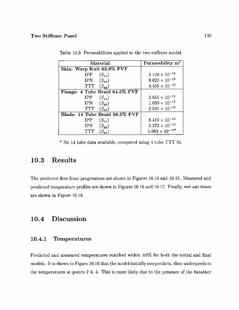
Two Stiffener Panel 130
Table 10.3: Permeabilities applied to the two stiffener model.
Material Permeability m 2
Skin: Warp Knit 63.9% FVF
IPP (S_z)
IPN (Sx_)
TTT (Sy_)
Flange: 4
Blade: 14
Tube Braid 64.5% FVF
IPP (S_)
IPN (Sy_)
TTT (Sx_)
Tube Braid 58.5% FVF
IPP (S_)
IPN (Syu)
TTT (S_)
2.129 x 10 -12
9.020 x 10 -13
4.456 x 10 -13
2.855 × 10 -12
1.039 X 10 -12
2.591 × 10 -13
8.419 x 10 -12
5.372 x 10 -12
5.983 x 10 -13.
* No 14 tube data available, computed using 4 tube TTT fit.
10.3 Results
The predicted flow front progressions are shown in Figures 10.14 and 10.15. Measured and
predicted temperature profiles are shown in Figures 10.16 and 10.17. Finally, wet out times
are shown in Figure 10.18.
10.4 Discussion
10.4.1 Temperatures
Predicted and measured temperatures matched within +6% for both the initial and final
models. It is shown in Figure 10.16 that the model initially overpredicts, then underpredicts
the temperatures at points 2 & 4. This is most likely due to the presence of the breather

Two Stiffener Panel 131
5825.
5436.
5048.
4660.
4271.
3883.
3495.
3106.
2718.
2330.
1942.
1553.
1165.
776.6
388.3
.0004272
Figure 10.14: Flow front progression in the initial model. The color bands represent the
flow front location at different times. The units are in seconds.

Two Stiffener Panel 132
X
Figure 10.15: Flow front progression in the final model. The color bands represent the
flow front location at different times. The units are in seconds.

Two Stiffener Panel 133
200
180
160
o 140
-_ 120
_)o_100EI- 80
6O
40
0
Temperature at points 2 & 4I | I I I
(::)_0 TC #2
TC #4
Initial model
Final model
I I I I I
50 1O0 150 200 250Time (min)
300
10
Error between measured and calculated temperatures at points 2 & 4I I I I I
a)
o_
-5
-10 ' ' ' ' '0 50 1O0 150 200 250 300
Time (min)
Figure 10.16: Measured and predicted temperatures at thermocouples 2 and 4. Thermo-
couple locations are shown in Figure 10.5.
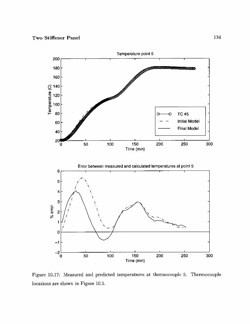
Two Stiffener Panel 134
200Temperature point 5
I I I I I
180
160
OvA140
120
_. 100
_- 8o
60
40
200
o--£) TC #5
,_ .... Initial Model
F,nal ModelI I I I I
50 1O0 150 200 250Time (min)
300
Error between measured and calculated temperatures at point 5i I i i I
o
5
4
3
2
1I
0
-1
-20
/ \
/ \
\
'\. " ,_, *
, \ / \.-I \. \
I l I I I
50 1O0 150 200 250Time (min)
300
Figure 10.17: Measured and predicted temperatures at thermocouple 5. Thermocouple
locations are shown in Figure 10.5.

Two Stiffener Panel 135
[] • [] [] [] []
I
C_
OJ
.o
0
0
Figure 10.18: Predicted and measured infiltration times for the two stiffener panel.

Two Stiffener Panel 136
material placedoverthe surfaceof the part when it wasautoclaved.The breather material
is aglassfiber cloth that has low thermal conductivity. Sincethe breatherwasnot included
in the model, it may be a sourceof error.
10.4.2 Fill Times
Figure 10.18 shows the wet out times for the various sensor locations. In the second
experimental run, the sensors wet out much sooner than the first run. Wet out times differ
by as much as 14% between the two runs. There seems to be some inherent variability in
the RFI process.
The model predictions were generally conservative in this case. All of the predicted wet
out times were longer than the experimentally measured times. The final model tended
to predict wet out sooner than the initial model. This is because of the more realistic
boundary conditions applied to the fully three dimensional model. The initial model had
only two temperature cycles applied (from TC #9 and #12). While this may have been
representative of the center section that the initial model was supposed to model, conduc-
tion from the ends of the model was neglected. Due to conduction, the final model tended
to be warmer overall than the initial model, therefore the final model would fill faster.
The closest match in wet out times was at location 4 where the prediction of the final
model was within 4% of the average of the experiments. The wet out times of the other
locations varied from 7% to 12%.

Two Stiffener Panel 137
10.5 Conclusions
When the correct thermal boundary conditions are applied to the model, the predicted
and experimental fill times agree well. The wet out times for the two experiments differed
by as much as 13%. Predicted wet out times were generally conservative. The model
overpredicted the wet out times by 7% to 12%.

Chapter 11
Conclusions and Future Work
11.1 Conclusions
This study has developed and verified a comprehensive three-dimensional RTM/RFI sim-
ulation model. The model can be used to simulate the precessing of complex shaped
composite structures including the flow of resin through a carbon fiber textile preform,
heat transfer in the preform/tool assembly, and cure kinetics of the resin.
The formulation for the flow model is given using the finite element/control volume (FE/CV)
technique based on Darcy's Law of creeping flow through a porous media. The FE/CV
technique is a numerically efficient method for finding the flow front location and the
fluid pressure. The heat transfer model is based on the three-dimensional, transient heat
conduction equation, including heat generation. Boundary conditions include specified
temperature and convection. The code was designed with a modular approach so the flow
and/or the thermal module may be turned on or off as desired. Both models are solved
sequentially in a quasi-steady state fashion.
A model was derived for the cure kinetics of the Hercules 3501-6 reduced catalyst resin.
138
Conclusions and Future Work 139
Severalexperimentswereperformedand computersimulationsof the experimentswererun
to verify the simulation model. Isothermal,non-reactingflowwassimulatedin a T-stiffened
section,and non-isothermal, reactive flow wassimulated in a steppedpanel and a panel
with two 'T' stiffeners. Flow front predicted times were generally within 5-15% of the
measuredtimes.
11.2 Future Work
Many of the necessary parameters needed by this model are not known with any degree
of certainty. Parameters include the permeability of the preform and the batch to batch
variability of this parameter, and the thermal conductivity of the preform material. The
resin model is also needs more study. The simulation model predicts resin flow at temper-
atures below 60°C, and experimental data supports this prediction. If flow in this range is
to be modeled, the resin model must be extended to even lower temperatures. Before this
simulation model can be used as a predictive tool, these inputs and their variation must
be known.
To increase the utility of the code, it should be extended to include the compaction be-
havior of the preform. This will allow the permeability of the preform to change and more
accurately reflect the actual processing conditions. This will increase the computational
resources. An important area of work will be finding either more efficient algorithms to
solve the problem, or adapting the current algorithms to multi-processor systems.

Bibliography
[1]
[2]
[3]
[4]
[5]
[6]
[7]
[8]
[9]
Macrae, J. D., "Development and Verification of a Resin Film Infusion/Resin Transfer
Molding Simulation Model for Fabrication of Advanced Textile Composites", Master's
thesis, Virginia Polytechnic Institute and State University, (1994).
Chen, V., A. Hawley, M. Klotzsche, A. Markus, and R. Palmer, "Composite Technol-
ogy for Transport Primary Structure", in First NASA Advanced Composite Technology
Conference, pp. 71-126, (1990).
Fracchia, C. A., J. Castro, and C. L. Tucker, "A Finite Element/Control Volume Sim-
ulation of Resin Transfer Mold Filling", in Proceedings of the American Society for
Composites, Fourth Technical Conference, pp. 157-166, (1989).
Day@, R., "A Unified Approach to Modeling Resin Flow During Composite Process-
ing", Journal of Composite Materials, vol. 24 (1991), pp. 22-41.
Friedrichs, B. and S. I. Gii_eri, "A Hybrid Numerical Technique to Model 3-D Flow
Fields in Resin Transfer Molding Process", Polymer Engineering and Science, vol. 35
(1995), no. 23, pp. 1834-1851.
Gauvin, "Permeability Measurement and Flow Simulation Through Fiber Reinforce-
ment", Polymer Composites, vol. 17 (1996), no. 1, pp. 34 42.
Loos, A. C. and J. D. MacRae, "A Process Simulation Model for the Manufacture of
a Blade-Stiffened Panel by the Resin Film Infusion Process", Composites Science and
Technology, vol. 56 (1996), pp. 273-289.
Cai, Z. and D. J. Lawrie, "A Simplified Mold Filling Program for the RTM Process",
in 2_th International SAMPE Technical Conference, pp. T675-T686, (1992).
Boccard, A., W. I. Lee, and G. S. Springer, "Model for Determining the Vent Locations
and the Fill Time of Resin Transfer Molds", Journal of Composite Materials, vol. 29
(1995), no. 3, pp. 306-333.
140

Bibliography 141
[10]
[11]
[12]
[13]
[14]
[15]
[16]
[17]
[18]
[19]
[2o]
[21]
[22]
Voller, V. R. and S. Peng, "An Algorithm for Analysis of Polymer Filling of Molds",
Polymer Engineering and Science, vol. 35 (1995), no. 22, pp. 1758-1765.
Calhoun, D. R., S. Yalva_, D. G. Wetters, C.-H. Wu, T. J. Wang, J. S. Tsai, and L. J.
Lee, "Mold Filling Analysis in Resin Transfer Molding", Polymer Composites, vol. 17
(1996), no. 2, pp. 251-264.
Lee, L. J., W. B. Young, and R. J. Lin, "Mold Filling and Cure Modeling of RTM and
SRIM Processes", Composite Structures, vol. 27 (1994), pp. 109-120.
Young, W.-B., "Three-Dimensional Nonisothermal Mold Filling Simulation in Resin
Transfer Molding", Polymer Composites, vol. 15 (1994), no. 2, pp. 118-127.
Loos, A. C., J. D. MacRae, D. Hood, D. E. Kranbuehl, and H. B. Dexter, "Resin
Film Infusion (RFI) Process Simulation of Complex Shaped Composite Structures", in
37th AIAA/ASME/ASCE/AHS/ASC Structures, Structural Dynamics and Materials
Conference, pp. 1828-1837, (April 1996).
Yoo, Y.-E. and W. I. Lee, "Numerical Simulation of the Resin Transfer Mold Filling
Process Using the Boundary Element Method", Polymer Composites, vol. 17 (1996),
no. 3, pp. 368-374.
Tucker, C. L., III, "Heat Transfer and Reaction Issues in Liquid Composite Molding",
Polymer Composites, vol. 17 (1996), no. 1, pp. 60-72.
Dessenberger, "Thermal Dispersion in Resin Transfer Molding", Polymer Composites,
vol. 16 (1995), no. 6.
Lin, R. J., L. J. Lee, and M. J. Liou, "Mold Filling and Curing Analysis in Liquid
Composite Molding", Polymer Composites, vol. 14 (1993), no. 1, pp. 71-81.
Chen, Y.-T. and C. W. Macosko, "Chemorheology of Polycyanate for Resin Trans-
fer Molding", in 24th International SAMPE Technical Conference, pp. T630-T644,
(1992).
Castro, J. M. and C. W. Macosko, "Studies of Mold Filling and Curing in the Reaction
Injection Molding Process", AIChE Journal, vol. 28 (1982), no. 2, pp. 250-260.
Reddy, J. N., An Introduction to the Finite Element Method, McGraw Hill, Inc., New
York, (1993).
Somanath, N. and A. C. Loos, "A Finite Element Cure Model and Cure Cycle Op-
timization of Composite Structures", Tech. Rep. CCMS-88-14, Virginia Tech Center
for Composite Materials and Structures, (1988).
Bibliography 142
[23]
[24]
[25]
[26]
[27]
[28]
[29]
[3o]
[31]
Osswald, T. A. and C. L. Tucker, "Compression Mold Filling Simulation for Non
Planar Parts", Intermational Polymer Processing V, (1990), pp. 79-87.
Baddourah, M. A., "Vector Sparse Solver (VSS) FORTRAN code", Written for NASA
Langley. Contact Olaf Storaasli at NASA Langley for further information.
Dexter, H. B., R. J. Palmer, and G. H. Hasko, "Mechanical Properties and Dam-
age Tolerance of Multiaxial Warp Knit Structural Elements", in Fourth NASA//DOD
Advanced Composites Technology Conference, NASA CP-3229, (June 7-11 1993).
Hinrichs, S., R. J. Palmer, A. Ghumman, J. Deaton, K. W. Furrow, and L. C.
Dickinson, "Mechanical Property Evaluation of Stitched/RFI Composites", in Fifth
NASA//DOD Advanced Composites Technology Conference, NASA CP-329_, (August
22-25,1994).
Furrow, K. W., "Material Property Evaluation of Braided and Braided/Woven Wing
Skin Blade Stiffeners", Contractor Report 198303, NASA, (April 1996).
Fingerson, J. C., A. C. Loos, and H. B. Dexter, "Verification of a Three-Dimensional
Resin Transfer Molding Prosess Simulation Model", Tech. Rep. CCMS-95-10, Virginia
Tech Center for Composite Materials and Structures, (September 1995).
Weideman, M. H., "An Infiltration/Cure Simulation Model for Manufacure of Fab-
ric Composites by the Resin Infusion Process", Master's thesis, Virginia Polytechnic
Institute and State University, (1992).
Hammond, V. H., A. C. Loos, H. B. Dexter, and G. H. Hasko, "Verification of a Two-
Dimensional Infiltration Model for the Resin Transfer Molding Prosess", Tech. Rep.
CCMS-93-15, Virginia Tech Center for Composite Materials and Structures, (Septem-
ber 1993).
Loos, A. C., M. H. Weideman, J. Edward R. Long, D. E. Kranbuehl, P. J. Kinsley,
and S. M. Hart, "Infiltration/Cure Modeling of Resin Transfer Molded Composites
Using Advanced Fiber Architectures", in First NASA Advanced Composite Technology
Conference, pp. 425-441, (1990).

Appendix A
Detailed Drawings of Tooling
Components
Detailed Drawings of Tooling Components
A.1 Stepped Panel Tooling Schematics
143

Detailed Drawings of Tooling Components 144
10"
,2 L
!
4" typ.
..@ , ..@I
5" typ.!
10"----_
_" 20"
30"
gee: ddettaall_ --7 7
to.,
! !
..@to.,
40" v
0.950" [!
O. 108" 08"
Figure A.I: Baseplate.
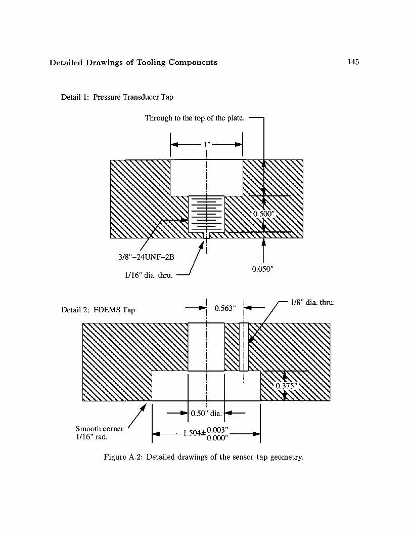
Detailed Drawings of Tooling Components 145
Detail 1: Pressure Transducer Tap
Through to the top of the plate. ----7
/L. _, ._1I- i -I
i
_/ " o.o o,,I
Detail 2: FDEMS Tap _ 0.563"i
I
it
IiiI
I
/I 'I
_ 0.50" dia. _
Smooth comer
1/16" rad. 1-"
,][_--'S 1/8" dia. thru.
I
i!I
I
+ 0.003" ..._I
1.504 0.000" "-1
Figure A.2: Detailed drawings of the sensor tap geometry.

Detailed Drawings of Tooling Components 146
A.2 Two Stringer Panel Tooling Schematics

Detailed Drawings of Tooling Components 147
24"
Pressure Transducer TapSee Below
I|
I|
Ii
3 3/4" .I
_ 5 1/2 O
i
,_------ 15" .----.--_i.,_ 15" ----------_
ie
Ii
48" r
Pressure Transducer Tap 3/8"-24UNF-2B
1/16" dia. thru. J '
Material: Aluminum
Figure A.3: Baseplate for the two stiffener panel.

Detailed Drawings of Tooling Components 148
24"
i-"
T'00'iyP" .
3. "N _"
t 0.350" typ.
7.000" --
0.25"R typ. ''I_
0.5"R typ. __
0.75" typ.
1/8" R typ.
J---_ 1.686" --typ.
Material: 606 l-T6
Figure A.4: Middle tool for the two stiffener panel. See Figure A.5 for sensor locations.

Detailed Drawings of Tooling Components 149
_1,, "J""--""1
.j------
Pressure
(
Taps
)
FDEMS Taps
"--1.
r
r
"---'1.
/.----
J
"--"L
J
Figure A.5: Sensor locations for the two stiffener panel.

Detailed Drawings of Tooling Components 150
24.000"
l 3.0!"
3.900"
I_., 4.840"I--
0.25"R typ. ''''_"
--lip
0.5"R
45*tyr
v\\
"t1/8" R 0.350"
.Jr I
0.75" typ.
Material: 6061-T6
Figure A.6: End tool for the two stiffener panel.

Detailed Drawings of Tooling Components 151
m _ m
k
24.000"
1
0.500"
_-_ r 0.672"
I I
tFigure A.7: Shim for the two stiffener panel.

Appendix B
Material Properties
Material Properties
B.1 Flow Properties
B.I.1 FVF
The fiber volume fraction (FVF) fit equation is:
v] = ao + alp + a2p 2 -t- a3p 3 + a4p 4 (B.1)
where vf is the FVF, ai are the fit constants, and p is the pressure measured in kPa.
Equation (B.1) is valid up the pressure 'Pmax' listed in the following table.
Note: The fit constants give a value for total FVF of the preform, not the carbon FVF.
The total FVF must be used as input to the permeability fits in the next section.
Tenax 8 Stack Warp Knit
AS4
14 Tube Braid
4 Tube Braid
ao al a2 a3 a4
X10 -4 xl0 -7 xl0 -10 X10 -14
0.50742 4.45047 -5.86561 3.57627 -8.12660
0.52491 3.23476 -4.19359 2.79126 -7.11793
0.55653 3.87254 -10.6127 15.6092 -82.2488
0.52363 5.23703 -11.8842 13.6207 -57.6054
Pma_
(kPa)
1515.
1450.
801.
922.
152

Material Properties 153
B.1.2 Permeability
The following equation is used to calculate permeabilities:
S = a(vf) b (B.2)
where S is the permeability in m 2, v I is the FVF, and a and b are the fit constants listed
in the following table.
To calculate the permeabilities at plus/minus one standard deviation, use:
S 4- a = exp [ln (avi b) t a'] (B.3)
where a' is the value listed in the following table.
Tenax 8 Stack Warp Knit 1
II to stitching
_L to stitchingTTT
AS4 6 stack 2
.2" 1/8"II to stitching
_L to stitching
TTT
14 Tube Braid 1
II to stitching
_1_to stitching
TTT
4 Tube Braid
II to stitching a
_L to stitching 1TTT 1
a b a'
9.03 x 10 -15 -12.18 0.1693
3.27 x 10 -15 -12.53 0.2800
1.26 x 10 -14 -7.95 0.1447
1.1 x 10 -15 -16.912
3.5 x 10 -16 -16.041
2.6 x 10 -14 -6.81
4.76 x 10 -1_ -18.26 0.1949
1.36 x 10 -16 -19.76 0.1477
2.5 x 10 -ls -16.05 -
9.8 x 10 -18 -15.88 -
5.88 x 10 -15 -8.63 0.1127
1Tamara Knott
2Tamara Knott, 8/19/97
3Tamara Knott, 9/8/97
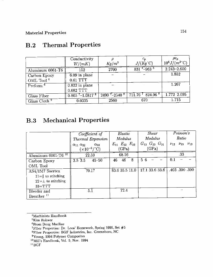
Material Properties 154
B.2 Thermal Properties
Conductivity p Cp pCp
W/(mK) Kg/m 3 J/(Kg°C) 106J/(m3°C)
Aluminum 6061-T6 152 2700 831 4-963 5 2.243-2.600
Carbon Epoxy
OML Tool 6
Preform 6
Glass Fiber
Glass Cloth 9
6.09 in plane
0.61 TTT
0.822 in plane
0.082 TTT
0.865 7-1.0817 s
0.0335
2490 7-2540 s
2560
711.76 7-824.96 s
670
1.852
1.267
1.772-2.095
1.715
B.3 Mechanical Properties
Coefficient of
Thermal Expansion
O_11 _22 C1_33
(xlO-°/°C)
Elastic Shear
1212
Modulus
E,1 E2_ E33(¢pa)
Modulus
G,2 G23 G3,(GPa)
Poisson's
Ratio
1223 1213
Aluminum 6061-T6 lo 22.59 68.26 - .33
Carbon Epoxy 3.5 3.5 45-50 46 46 8 5-6 - - 0.1 - -
OML Tool
?0.1? 83.6 35.5 11.0 17.1 33.6 33.6 .403.390.390
5.1
AS4/IM7 Saertex
11=11 to stitching
22=_1_ to stitching
33=TTT
72.4Bleeder and
Breather 11
4Machinists Handbook
5Kim Rohwer
6From Doug MacRae
7Fiber Properties: Dr. Loos' Homework, Spring 1995, Set #5
SFiber Properties: BGF Industries, Inc. Greensboro, NC
9Young, 1994 Polymer Composites
1°Mill's Handbook, Vol. 5, Nov. 1994
11BGF