66

Residues (Total Dissolved Solids (TDS) and Total Suspended Solids (TSS))

Total Dissolved Solids measures the solids remaining in a water sample filtered through a 1.2 µm

filter. According to the World Health Organization (WHO, 1996), the compounds and elements

remaining after filtration are commonly calcium, magnesium, sodium, potassium, carbonate, bicarbonate,

chloride, sulfate, silica and nitrate-n. High TDS affects the taste and odor of water and in general, levels

above 300 mg/L become noticeable to consumers. As TDS increases, the water becomes increasingly

unacceptable. Although the SMCL for TDS is 500 mg/L, levels above 1200 mg/L are unacceptable to

most consumers. Because TDS measurements may include a variety of parameters which can be

naturally occurring or anthropogenic, its value as an indicator of nonpoint source pollution is limited.

Median values of TDS were found below the SMCL of 500 mg/L, but outliers were common,

especially in the Bluegrass (Figure 34). TDS was surprisingly low in the Mississippian Plateau,

Figure 34. Boxplot for TDS measurement distributions in BMU #2

67

especially considering that this is soluble carbonate terrane. One possible explanation is that the quick

flow characteristics of this region reduce the contact time between water and rock, thereby retarding

dissolution. In general, TDS is not usually an important primary indicator of nonpoint source pollution of

groundwater, although this parameter can serve as a surrogate indicative of general water quality.

Because no probable sources for elevated TDS were noted adjacent to sampling sites, no nonpoint source

impacts could be confirmed. Figure 35 shows higher values in the Bluegrass and Ohio River Alluvium.

These higher values are probably natural, resulting from longer residence times, which allow for more

dissolution in these areas.

Total Suspended Solids (TSS), also known as non-filterable residue, are those solids (minerals

and organic material) that remain trapped on a 1.2 µm filter (U.S.EPA, 1998). Suspended solids can enter

groundwater through runoff from industrial, urban or agricultural areas. Elevated TSS (MMSD, 2002)

can “. . . reduce water clarity, degrade habitats, clog fish gills, decrease photosynthetic activity and cause

an increase in water temperatures.” TSS has no drinking water standard. Therefore, data in this report

are compared to the KPDES surface water discharge permit requirement for sewage treatment plants of

35 mg/L.

Approximately 57% of the samples analyzed detected TSS, with about 6% of the detections

above 35 mg/L. Most values occurred within a narrow range, but outliers were common (Figure 36). In

general, TSS is not usually considered a good indicator for nonpoint source pollution in groundwater.

However, in some karst systems, turbidity and TSS vary with change in flow. Poor management

practices associated with activities such as construction and agricultural tillage can strip vegetation and

allow the quick influx of sediment into groundwater via overland flow. Therefore, outliers in the karst of

the Bluegrass and Mississippian Plateau may represent nonpoint source impacts. Typically, given the

nature of the activities that introduce sediments into karst groundwater, these impacts are transient. In the

Eastern Coal Field, however, high TSS values are more difficult to interpret. Outliers here may represent

sloughing of unstable beds within the well bore or possibly failure of the well's annular seal.

Figure 35. Map of Total Dissolved Solids data for BMU 2

69

Figure 36. Boxplot for TSS measurement distributions in BMU #2

Figure 37 illustrates that high levels of TSS generally occur in karst areas where aquifers can be

under the direct influence of surface water runoff.

Nutrients Nutrients included in this report are nitrate-nitrogen, nitrite-nitrogen, ammonia, orthophosphate

and total phosphorous. Nutrients are particularly important in surface water, where they are the main

contributors to eutrophication, which is excessive nutrient enrichment of water. This enrichment can

cause an overabundance of some plant life, such as algal blooms and may also have adverse effects on

animal life, because excessive oxygen consumption by plants leaves little available for animal use. In

addition to comparisons with various water quality standards, nutrient data from sites in this study were

compared to the two reference springs.

Figure 37. Map of Total Suspended Solids data for BMU 2

71

Nitrate (NO3) occurs in the environment from a variety of anthropogenic and natural sources:

nitrogen-fixing plants such as alfalfa and other legumes, nitrogen fertilizers, decomposing organic debris,

atmospheric deposition from combustion and human and animal waste. Nitrate is reported either as the

complex ion NO3, or as the equivalent molecular nitrogen-n. Since 1 mg/L of nitrogen equals 4.5 mg/L

nitrate; therefore, the drinking water MCL of 10 mg/L nitrate-n equals 45 mg/L nitrate. In this report,

results are reported as "nitrate-n."

In infants, excess nitrate consumption can cause methemoglobinemia or "blue-baby" syndrome.

In adults, possible adverse health effects of nitrate ingestion are under study and much debated. Because

nitrate is difficult to remove through ordinary water treatment, its occurrence at levels above the MCL in

public water systems is a problem.

As shown in Figure 38 and in the Nutrients Summary Statistics table in Appendix F, median

Figure 38. Boxplot for Nitrate-Nitrogen measurement distributions in BMU #2

72

values of nitrate-n varied from a low of 0.1785 mg/L in the Eastern Coal Field to a high of 5.58 mg/L in

the Ohio River Alluvium. Median values for the Bluegrass and the Mississippian Plateau were 2.76 mg/L

and 0.9025 mg/L respectively. Approximately 4.48% of nitrate-n detections were found above the MCL

of 10.0 mg/L and these exceedances occurred in the Bluegrass and Ohio River Alluvium. No MCL

exceedances occurred in the Eastern Coal Field or the Mississippian Plateau.

Nitrate-n values found in this study were compared to the values found in other studies, as well as

those from reference springs (Table 2). Based upon nitrate-n data from throughout the United States

(USGS, 1984), most researchers believe that nitrate-n levels of 3.0 mg/L or lower represent background

levels. However, in Kentucky some nitrate-n data support significantly lower levels for ambient

conditions. For example, a review of nitrate-n analyses from three reference springs (Table 2) shows a

median value of 0.1805 mg/L for these sites. In addition, Carey and others (1993) found a median of 0.71

mg/L for nitrate-n in 4,859 groundwater samples collected from predominantly domestic water wells

throughout the state. In their statewide study of nitrate-n, Conrad and others (1999) found that depth was

a determining factor regarding the occurrence of nitrate-n in groundwater. MCL exceedances occurred

most frequently in shallow dug wells and declined with depth. Nearly 10% of dug wells exceeded the

MCL; whereas only about 1% of wells greater than 151 feet were in exceedance and median values were

only 0.6 mg/L. In conclusion, the median value of 2.38 mg/L for nitrate-n found in this study is well

above background levels and indicates probable nonpoint source impact on groundwater in all

physiographic provinces except the Eastern Coal Field.

Figure 39 indicates that urban areas have comparable or higher levels than agricultural areas,

which was an unexpected result. This higher than expected occurrence of nitrate-n in urban areas may be

the result of leakage from sanitary sewers combined with infiltration from the application of nitrogen-

based lawn fertilizers. Forested areas showed the lowest median values of nitrate-n but unexpected

outliers occurred, several of which approach the MCL, with one exceeding that value. These higher

values may be the result of nearby failing septic systems, which could allow untreated waste to

73

Figure 39. Boxplot for Nitrate-Nitrogen Distributions by Land Use in BMU #2.

infiltrate into the groundwater. High nitrate-n values in agricultural areas are expected and are the result

of the application of nitrogen fertilizers combined with livestock grazing and feeding operations.

Figure 40 shows the geographical distribution of nitrate-n values in BMU 2. High values in wells

in the Ohio River Alluvium and in springs, especially in the Bluegrass, were observed. The highest value

found in this study (19.8 mg/L) occurred at a spring in western Fleming County and is probably the result

of intense livestock grazing in the area immediately upgradient of the spring.

Nitrite (NO2) also occurs naturally from most of the same sources as nitrate. However, nitrite is

an unstable ion and is usually quickly converted to nitrate in the presence of free oxygen. The MCL for

nitrite-n is 1 mg/L.

Figure 40. Map of Nitrate data for BMU

75

Nitrite-n was found to occur at very low levels and with several outliers, as shown in Figures 41

and 42. Nitrite-n was not detected above the MCL and the highest values were less than half the MCL of

Figure 41. Boxplot for Nitrite-Nitrogen measurement distributions in BMU #2

Figure 42. Boxplot for Nitrite-Nitrogen Distribution by Land Use in BMU #2

76

1 mg/L. The lowest median value found in this study was 0.001165 mg/L in the Eastern Coal Field

(Appendix F, Nutrients Summary Statistics Table). Values almost as low occurred in the Ohio River

Alluvium and the Bluegrass: 0.002 mg/L. The highest median value of 0.00375 mg/L occurred in the

Mississippian Plateau.

In the environment, nitrite-n generally converts rapidly to nitrate through oxidation, which this

study reflects. Nitrite is not a significant nonpoint source pollutant, although it may contribute to high

levels of nitrate. In this study, the occurrence of nitrite-n was not dependent on land use, as shown in

Figure 42. In addition, Figure 43 further supports the conclusion that no significant problem with

nonpoint source pollution from nitrite-n was found in this study. However, when viewed together nitrate-

n and nitrite-n do have broad nonpoint source impacts.

Ammonia (NH3) occurs naturally in the environment, primarily from the decay of plants and

animal waste. The principal source of man-made ammonia in groundwater is from ammonia-based

fertilizers. No drinking water standards exist for ammonia; however, the proposed DEP limit for

groundwater is 0.110 mg/L.

Reference spring data (Table 2) shows that ammonia values are typically very low, often below

the method detection limit of 0.02 mg/L. Low values, but above this level, may indicate natural

variations. However, increasing values, as shown in the outliers in Figures 44 and 45 seem to indicate

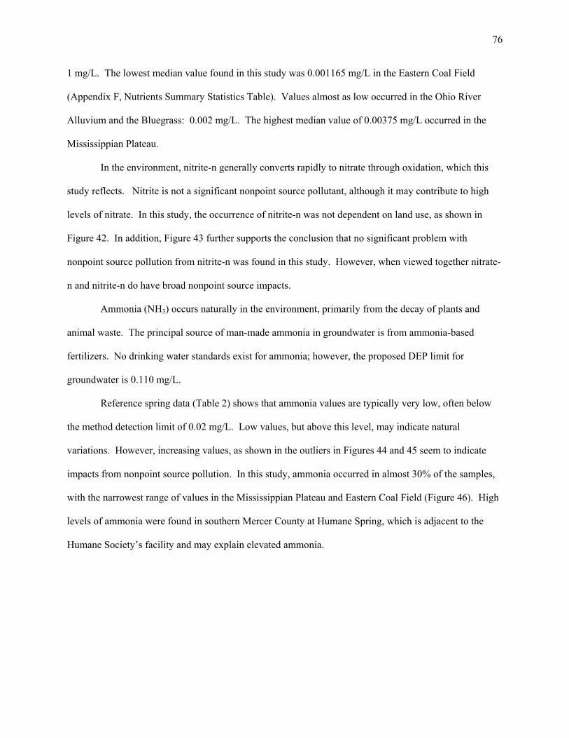
impacts from nonpoint source pollution. In this study, ammonia occurred in almost 30% of the samples,

with the narrowest range of values in the Mississippian Plateau and Eastern Coal Field (Figure 46). High

levels of ammonia were found in southern Mercer County at Humane Spring, which is adjacent to the

Humane Society’s facility and may explain elevated ammonia.

Figure 43. Map of Nitrite-n data for BMU 2

78

Figure 44. Boxplot for Ammonia measurement distributions in BMU #2

Figure 45. Boxplot for Ammonia Distribution by Land Use in BMU #2.

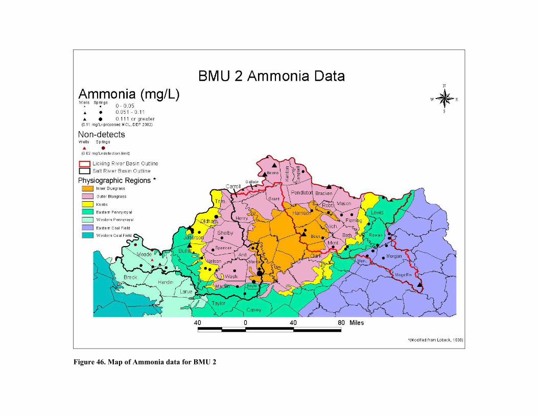
Figure 46. Map of Ammonia data for BMU 2

80

Two forms of phosphorus are discussed in this report: orthophosphate-p and total phosphorus.

Orthophosphate-P (PO4 -P), or simply "orthophosphate,” or "ortho-p,” is the final product of the

dissociation of phosphoric acid, H3PO4. It occurs naturally in the environment most often as the result of

the oxidation of organic forms of phosphorus; it is found in animal waste and in detergents.

Orthophosphate is the most abundant form of phosphorus, usually accounting for about 90% of the

available phosphorus. Phosphorus contributes to the eutrophication of surface water, particularly lakes,

commonly known as "algal blooms".

The most common phosphorus mineral is apatite [Ca5(PO4)3(OH,F,Cl)], which is found in the

phosphatic limestones in the Bluegrass. Neither orthophosphate nor total phosphorus has a drinking

water standard. Orthophosphate data are compared to the Texas surface water quality standard of 0.04

mg/L and total phosphorus data to the surface water limit of 0.1 mg/L recommended by the USGS.

In natural systems relatively unimpacted from anthropogenic sources, orthophosphate occurs at

very low levels. For example, reference reach springs typically were either non-detect for ortho-p, or had

values in the range of 0.002 – 0.004 mg/L. Although some more sensitive laboratory methods were used

in this study, the most common MDL was 0.059 mg/L, which is above the surface water quality standard

of 0.04 mg/L used for comparison in this study. Because approximately 70% of the samples were non-

detect using that relatively high detection limit, the narrow range of values shown in Figure 47 may not

reflect the true occurrence of orthophosphate in this area. In the Bluegrass, numerous high outliers of

orthophosphate may be the result of naturally occurring phosphatic limestones and from agricultural

practices, including livestock production and grazing or the application of phosphate-rich fertilizers.

Therefore, this may indicate possible nonpoint source pollution. Higher median values of orthophosphate

in urban areas, as shown in Figure 48, probably reflect impacts from leaking sanitary sewers. A map

illustrating the distribution of orthophosphate data is presented in Figure 49, which shows that most of the

higher values occur within the Bluegrass.

81

Figure 47. Boxplot for Orthophosphate measurement distributions in BMU #2

Figure 48. Boxplot for Orthophosphate Distribution by Land Use in BMU #2

Figure 49. Map of Orthophosphate data for BMU 2

83

Total phosphorus is the sum of organic and inorganic forms of phosphorus. Total phosphorus in

reference reach springs was usually nondetect, using an MCL of 0.05 mg/L. Low amounts of phosphorus

within a narrow range occur in BMU 2, except for the Bluegrass (Figure 50). Phosphatic

Figure 50. Boxplot for Total Phosphorus measurement distributions in BMU 2

limestones are well known in the Bluegrass (McDowell, 2001). Therefore, in the Bluegrass the most of

the variability of this parameter is probably the result of natural variability in the system, with some

possible introduction from anthropogenic sources. As expected, forested areas show the lowest levels of

total phosphorus, as shown in Figure 51. Agricultural and urban areas showed only slightly greater

levels, indicating possible nonpoint source impacts from animal waste in agricultural areas and human

waste and phosphatic detergents from sanitary sewer leaks, as well as the application of lawn fertilizer, in

urban areas. Figure 52 shows the distribution of total phosphorus in BMU 2.

84

Figure 51. Boxplot of Total Phosphorus Distribution by Land Use in BMU #2.

Figure 52. Map of Total Phosphorus data for BMU 2

86

Volatile Organic Compounds

The volatile organic compounds most often detected in groundwater are the BTEX compounds:

benzene, toluene, ethylbenzene and xylenes. Also of concern is methyl-tertiary-butyl-ether, or MTBE.

Because these compounds are among the most commonly found hazardous components of gasoline (Irwin

and others, 1997) and because of potential acute and long-term impacts to aquatic life and human health,

they are included in this report. Although BTEX compounds also occur naturally, their occurrence in

groundwater is usually indicative of point source contamination, most often leaking underground storage

tanks.

In urban areas, nonpoint sources of BTEX and MTBE include leaks from automobile gas tanks.

Some researchers are concerned with possible air-borne deposition of BTEX and MTBE from the

incomplete combustion of fossil fuels. An additional potential source is from pesticides that may contain

volatile organic compounds, including BTEX, used as carriers for the active ingredient. These volatile

organic compounds are important to evaluate because of various detrimental effects to human health and

the environment.

BTEX and MTBE are persistent in the environment, particularly groundwater, for two primary

reasons. First, water solubility of BTEX is moderate to high, ranging from a low of 161 mg/L for

ethylbenzene to 1730 mg/L for benzene. In comparison, MTBE is very soluble, with values from 43,000

mg/L to 54,300 mg/L. Because of this solubility, MTBE in contaminant plumes moves at virtually the

same rate as the water itself, whereas BTEX plumes move at somewhat slower rates. Second, because

these compounds (except for benzene) have relatively low vapor pressure and Henry’s law constants, they

tend to remain in solution, rather than being volatilized.

Because of these and other, physical and chemical characteristics, clean up of contaminated

groundwater is difficult. “Pump and treat” and various bioremediation techniques have proven the most

useful techniques.

87

Benzene

Benzene is found naturally in the environment in organic matter, including coal and petroleum

and is released into the environment during combustion. Benzene is also found in products manufactured

from crude oil, including gasoline, diesel and other fuels, plastics, detergents and pesticides. Benzene is

also produced during the combustion of wood and vegetation. Benzene is a known carcinogen in humans

and has been associated with various nervous system disorders, anemia and immune system depression

(U.S.EPA, 2000). The MCL for benzene is 0.005 mg/L.

Benzene was detected at only two locations (Figures 53 and 54) in this study: Humane Spring in

Figure 53. Boxplot for Benzene measurement distributions in BMU #2

Mercer County and at a public water supply well (since abandoned) in Meade County. Both occurrences

are from known point sources. For benzene, this study found no nonpoint source impacts from urban run-

off.

Figure 54. Map of BTEX and MTBE data for BMU 2

89

Toluene is a clear liquid that occurs naturally in crude oil, as well as in refined oil products, such

as gasoline. Toluene also occurs naturally in coal and is common in paints, paint thinner, fingernail

polish and other products. Although toluene is not considered carcinogenic in humans (U.S.EPA, 2000),

it has been linked with several detrimental physical and neurological effects, including diminished

coordination and the loss of sleep ability. Toluene has an MCL of 1.0 mg/L.

In this study, toluene was detected at the same two sites as benzene (Figure 55). Because these

Figure 55. Boxplot for Toluene measurement distributions in BMU #2

sites are known point sources, no nonpoint source impacts to groundwater from this parameter were found

in this study.

Ethylbenzene is a component of crude oil and is a constituent of refined petroleum products,

including gasoline. In addition, this colorless liquid is used to manufacture styrene. According to the

U.S.EPA (2000), limited studies of ethylbenzene have shown no carcinogenic effects in humans;

however, animal studies have shown detrimental health effects to the central nervous system. The MCL

for

90

ethylbenzene is 0.7 mg/L. Ethylbenzene was detected only at Humane Spring (see Figure 54 for

reference) as shown in Figure 56. As with the other volatile organic compounds included in this report,

Figure 56. Boxplot for Ethylbenzene measurement distributions in BMU #2

this occurrence is from a known point source and therefore no nonpoint source impacts to groundwater

were found in this BMU.

Xylenes are any one of a group of organic compounds typically found in crude oil, as well as in

refined petroleum products such as gasoline. Xylenes are clear and sweet-smelling. They are used as

solvents and in the manufacture of plastics, polyester and film. Xylenes have an MCL of 10 mg/L. They

are not carcinogenic in humans, although data are limited. In humans, exposure to excessive amounts is

associated with disorders of the central nervous system, kidneys and liver (U.S.EPA, 2000). Xylenes

were detected only at Humane Spring and the Meade County well (see Figures 54 and 57). Again, these

occurrences are from known point sources; therefore, no nonpoint source impacts from this volatile

organic compound were found.

91

Figure 57. Boxplot for Xylenes measurement distributions in BMU #2

Methyl-tertiary-butyl-ether, or MTBE, is a man-made compound and does not occur naturally. It

is used as an oxygenate added to gasoline in order to promote more complete combustion, increase octane

and to reduce emissions of carbon monoxide and ozone. MTBE is very mobile in groundwater and has

contaminated numerous aquifers throughout the United States. This compound has no MCL; however,

the proposed DEP standard is 0.05 mg/L. According to the U.S.EPA (1997), no studies have

documented human health effects from the consumption of MTBE-contaminated water. However, animal

studies have shown some carcinogenic and non-carcinogenic effects.

One sample in 81 analyses detected a trace of MTBE. In this sample, the volume remaining after

other volatile organic analyses were performed was too low for a precise value to be determined:

therefore, an estimated value of 0.00042 mg/L was assigned. This concentration, however, is lower than

the detection limits used for the 80 other samples analyzed. These detection limits were 0.001 mg/L, 0.02

mg/L and 0.2 mg/L. No MTBE occurred in any other sample in this study, using these various detection

limits. Because MTBE was detected in only one sample, at Jesse's Spring in Louisville, no boxplot is

92

presented. However, the map presented in Figure 54 shows this occurrence. This occurrence may be due

to urban runoff, or possibly atmospheric deposition, but because no other volatile organic compounds

were detected, any conclusions for this single estimated detection are tentative at best.

CONCLUSIONS Although limited in scope, this study adds valuable data to the existing body of knowledge

regarding groundwater in the state in general and this BMU in particular. This additional information will

assist efforts to understand and manage this resource.

As mentioned above, differentiating between substances that are naturally-occurring and those

that impact groundwater through nonpoint source pollution is sometimes difficult. For parameters that

are man-made, such as pesticides and MTBE, the determination of nonpoint source pollution can be

readily made; however, for parameters that also occur naturally, such as metals and nutrients, such a

determination is problematic. For these parameters, data from this study of BMU 2 can be compared with

data from reference reach springs and the statewide ambient network, as well as with data published by

other researchers. Through these comparisons, tentative conclusions can be made.

Table 7 summarizes the conclusions reached in this study. This table categorizes impacts to

groundwater from various nonpoint sources as "Definite”, "Possible”, or as not existing or simply as

"No”.

A "Definite" impact is defined as an occurrence or detection of an unnatural parameter, such as a

pesticide, or the detection of a compound that is both naturally occurring and anthropogenic, such as

nitrate-n, that far exceeds background concentrations, as determined by comparison with reference site

data or data from other groundwater studies. Whether such impacts are detrimental would require

receptor studies outside the scope of this particular inquiry. Definite nonpoint source impacts to

groundwater were documented for the following parameters: nitrate-n and several herbicides, including

atrazine, metolachlor, alachlor and simazine.

93

Table 7. Nonpoint Source Impacts to Groundwater, BMU 2

PARAMETER

NO NPS INFLUENCE ON

GROUNDWATER QUALITY

POSSIBLE NPS INFLUENCE ON

GROUNDWATER QUALITY

DEFINITE NPS INFLUENCE ON

GROUNDWATER QUALITY

Conductivity • Hardness (Ca/Mg) •

Bulk Water Quality

Parameters PH • Chloride • Fluoride • Inorganic

Ions Sulfate • Arsenic • Barium • Iron • Manganese •

Metals

Mercury • Ammonia • Nitrate-n • Nitrite-n • Orthophosphate •

Nutrients

Total phosphorous • Alachlor • Atrazine • Cyanazine • Metolachlor •

Pesticides

Simazine • Total Dissolved Solids • Residues Total Suspended Solids • Benzene • Ethylbenzene • Toluene • Xylenes •

Volatile Organic

Compounds MTBE •

A "Possible" impact is a tentative category for those parameters that occur both naturally as well

as from anthropogenic sources. These impacts are difficult to assess and at this time only tentative

conclusions can made. Possible nonpoint source impacts to groundwater were found for several

nutrients, including ammonia, total phosphorus and orthophosphate; and for total suspended solids and

total dissolved solids. The latter two parameters in particular are difficult to assess because they each

measure numerous elements and compounds, rather than discrete ones.

Parameters with "No" significant impacts to groundwater were: 1) either not detected; 2) were

detected in a limited number of samples or at very low values, such as mercury; or 3) are thought to

occur at natural levels. This study concluded that No impacts to groundwater were apparent for the

following parameters: conductivity, hardness, chloride, fluoride, sulfate, arsenic, barium, iron,

94

manganese, mercury, nitrite-n, cyanazine, BTEX and MTBE. (Note that although BTEX compounds

occurred at two sites, these are the result of known point sources and therefore not indicators of nonpoint

source pollution. The source of the single occurrence of MTBE at one site in Louisville is unexplained,

as previously noted.)

Several biases inherent in any sampling program are a concern in the design, implementation and

analysis of results. Most importantly, personnel and funding limit both the geographical distribution of

sites, as well as the sampling schedule itself. Therefore, only one site per approximately 100 square miles

could be sampled. Temporal variations, which are important in all groundwater systems, but especially in

quick flow karst systems, may not be adequately addressed through a quarterly sampling schedule over

one year's time. Another bias of the study was that there were no wells sampled in the Mississippian

Plateau. Although these problems may preclude definitive conclusions regarding short-term changes in

groundwater quality, this project and others like it, contribute vital data that add to our continued

incremental understanding of this resource.

The authors recommend that additional groundwater studies continue, including expansion of the

statewide ambient program and more focused nonpoint source projects in order to continue the

characterization, protection and management of this resource. In particular, continued studies should

focus on increasing the density of sampling sites as well as addressing temporal water quality variations,

especially in karst terrane.

Based upon a review of groundwater data from this study in conjunction with surface water data,

several areas in BMU 2 will receive additional monitoring in the next cycle of the watershed management

system: Sinking Creek, Beargrass Creek and selected portions of the Licking River. In the Sinking Creek

area, additional dye tracing will further define groundwater basins, and water quality studies will focus on

pesticides, nutrients and pathogens. Beargrass Creek, in urban Jefferson County, has been impaired

through urban runoff and possibly leaking sewers; therefore, further groundwater studies in this area will

focus on these impacts. In the Licking River basin, the GWB will sample areas lacking groundwater

quality data.

i

LITERATURE CITED ATSDR, 2001, ToxFAQ, cited July 2002, http://www.atsdr.cdc.gov/toxfaq.html. Brosius, L., 2001, STA 215, unpublished lecture notes, Richmond, Ky., Eastern Kentucky University, 2 p. Blanset, J. and Goodmann, P. T., 2002, Arsenic in Kentucky's Groundwater and Public Water Supplies,

Geological Society of America, Abstracts with Programs Vol. 34, No. 2, March 2002, Abstract No: 32458.

Carey, D. I. and Stickney, J. F., 2001, County Ground-Water Resources in Kentucky, Series XII, 2001, Cited December 2002, http://www.uky.edu/KGS/water/library/webintro.html Carey, D. I., Dinger, J. S., Davidson, O. B., Sergeant, R. E., Taraba, J. L., Ilvento, T. W., Coleman, S.,

Boone, R. and Knoth, L. M., 1993, Quality of Private Ground-Water Supplies in Kentucky, Information Circular 44 (series 11), 155p.

Conrad, P. G., Carey, D. I., Webb, J. S., Fisher, R. S. and McCourt, M. J., 1999a, Ground-Water Quality

in Kentucky: Fluoride, Information Circular 1 (series 12), 4 p. Conrad, P. G., Carey, D. I., Webb, J. S., Dinger, J. S. and McCourt, M. J., 1999b, Ground-Water Quality

in Kentucky: Nitrate-Nitrogen, Information Circular 60 (series 11), 4 p. Currens, J. C., Paylor, R. L. and Ray, J. A., 2002, Mapped Karst Ground-Water Basins in the Lexington

30 x 60 Minute Quadrangle, Map and Chart Series 35 (Series XII), scale 1:100,000. Currens, J. C. and Ray, J. A., 1998, Mapped Karst Ground-Water Basins in the Harrodsburg 30 x 60

Minute Quadrangle, Map and Chart 16 (Series XI), scale 1:100,000. Currens, J. C. and McGrain, P., 1979, Bibliography of Karst Geology in Kentucky, Special Publication 1

(series 11), 59 p. Driscoll, F. G., 1986, Groundwater and Wells, Johnson Division, St. Paul, Minn., 1089 p. Faust, R. J., Banfield, G. R. and Willinger, G. R., 1980, A Compilation of Ground Water Quality Data for

Kentucky, USGS Open File Report (OFR 80-685), 963 p. Fetter, C. W., 1992, Contaminant Hydrogeology: New York, Macmillan, 458 p. Fisher, R. S., 2002, Ground-Water Quality in Kentucky: Arsenic, Information Circular 5 (series 12), 4 p. Hall, B., 2002, Statistics Notes, cited June 2002,

http://bobhall.tamu.edu/FiniteMath/Module8/Introduction.html. Hayes, T. B., Collins, A., Lee, M., Mendoza, M., Noriega, A., Stuart, A. and Vonk, A., 2002,

Hermaphroditic, demasculinized frogs after exposure to the herbicide atrazine at low ecologically relevant doses, Proceedings of the National Academy of Sciences, PNAS 2002 99, p. 5476-5480.

Hem, J., 1985, Water-Supply Paper 2254, USGS, 263 p., cited May 2002,

http://water.usgs.gov/pubs/wsp/wsp2254/.

ii

Irwin, R. J., Mouwerik, M. V., Stevens, L., Seese, M. D. and Basham, W., 1997, Environmental Contaminants Encyclopedia Entry for BTEX and BTEX Compounds, National Park Service, Water Resources Division, Water Operations Branch, Fort Collins, Colo., 35 p., cited December 2002: http://www.nature.nps.gov/toxic/list.html

Keagy, D. M., Dinger, J. S., Hampson, S. K. and Sendlein, L. V. A., 1993, Interim Report on the

Occurrence of Pesticides and Nutrients in the Epikarst of the Inner Blue Grass Region, Bourbon County, Kentucky, Open-File Report OF-93-05, 22 p.

Kentucky Department of Agriculture, 2000, Fourth Quarter Report (Year End) 2000, 106 p. Kentucky Division of Water, 2002a, cited May 2002, http://kywatersheds.org/Kentucky. Kentucky Division of Water, 2002b, unpublished Alphabetical Listing of Active Public Water Systems,

March 26, 2002, 14 p. Kentucky Division of Water, 2002c, Kentucky Ambient/Watershed Water Quality Monitoring Standard

Operating Procedure Manual, 39 p. Kentucky Geological Survey, 1969, Index to Hydrologic Atlases for Kentucky, 1 p. Kentucky Geological Survey, 1993, Index to Geologic Maps for Kentucky, Misc. Map 27 (series 10), 1 p. Kentucky Department for Environmental Protection (compiler), 2002, digital land-use and physiographic

province maps, cited May 2002, http://www.nr.state.ky.us/nrepc/ois/gis/library/statedocs. Kentucky Department of Mines and Minerals, 2002, Annual Reports 1996-2001, cited November 2002,

http://www.caer.uky.edu/kdmm/homepage.htm Kipp, J. A. and Dinger, J. S., 1991, Stress-Relief Fracture Control of Ground-Water Movement in the

Appalachian Plateaus, Reprint 30 (series 11), 11 p. Lobeck, A. K., 1930, The Midland Trail in Kentucky: a physiographic and geologic guide book to US

Highway 60, KGS Report Series 6, pamphlet 23. McDowell, R. C. (ed.), 2001, The Geology of Kentucky, USGS Professional Paper 1151 H, on-line

version 1.0, cited May 2002, http://pubs.usgs.gov/prof/p1151h. Milwaukee Metropolitan Sewerage District (MMSD), 2002, Environmental Performance Report-2002,

cited December 2002, http:// www.mmsd.com/envper2001/page3.asp Minns, S. A., 1993, Conceptual Model of Local and Regional Ground-Water Flow in the Eastern

Kentucky Coal Field, Thesis 6 (series 11), 194 p. Noger, M. C.(compiler), 1988, Geologic Map of Kentucky, scale 1:250,000. Ohio River Valley Sanitation Commission (ORSANCO), 2002, cited May 2002,

http://www.orsanco.org/rivinfo. Quinlan, J. F. (ed.), 1986, Practical Karst Hydrogeology, with Emphasis on Groundwater Monitoring,

National Water Well Association, Dublin, Ohio, 898 p.

iii

Ray, J. A., Webb, J. S. and O'dell, P. W., 1994, Groundwater Sensitivity Regions of Kentucky, Kentucky Division of Water, scale 1:500,000.

Tuttle, M. L. W., Goldhaber, M. B. and Breit, G. N., 2001, Mobility of Metals from Weathered Black

Shale: The Role of Salt Efflorescences, (abs.) Geological Society of America, Annual Meeting, 2001, cited May 2002, http://gsa.confex.com/gsa/2001AM/finalprogram/abstract 26237.htm.

U.S.EPA, 1997, Drinking Water Advisory: Consumer Acceptability Advice and Health Effects Analysis

on Methyl-Tertiary-Butyl-Ether, Dec. 1997, EPA 822/F-97-008, cited August 2002, http://www.epa.gov/waterscience/drinking/mtbefact.pdf

U.S.EPA, 1998, Total Suspended Solids Laboratory Method 160.2, cited August 2002:

http://www.epa.gov/region09/lab/sop U.S.EPA, 2000, Drinking Water Standards and Health Advisories, cited June 2002, http://www.epa.gov/ost/drinking/standards/dwstandards.pdf. U.S.EPA, 2002a, Drinking Water Priority Rulemaking: Arsenic, cited July 2002,

http://www.epa.gov/safewater/ars/arsenic.html. U.S.EPA, 2002b, Drinking Water and Health, cited July 2002, http://www.epa.gov/safewater. United States Geological Survey, 1984, Overview of the Occurrence of Nitrate in Ground Water of the

United States: USGS National Water Summary 1984; USGS Water-Supply Paper 2275, pages 93-105.

United States Geological Survey, 2002a, Groundwater quality information, cited May 2002,

http://co.water.usgs.gov. United States Geological Survey, 2002b, Coal Quality Data, cited May 2002,

http://energy.er.usgs.gov/products/databases/coalqual. Water Quality Association, 2002, Hardness Chart, cited July 2002, http://www.wqa.org. World Health Organization, 1996, Guidelines for drinking water quality, 2nd edition, cited August 2002,

http://www.who.int/water_sanitation_health/. Wunsch, D. R., 1991, High Barium Concentrations in Ground Water in Eastern Kentucky, Kentucky

Geological Survey Reprint R-31 (series 11), 14 p.