Full Terms & Conditions of access and use can be found athttp://www.tandfonline.com/action/journalInformation?journalCode=trsl20

Download by: [200.196.107.27] Date: 20 February 2016, At: 16:55

Remote Sensing Letters

ISSN: 2150-704X (Print) 2150-7058 (Online) Journal homepage: http://www.tandfonline.com/loi/trsl20

Field measurements of the backscatteringcoefficient in a cascading reservoir system: firstresults from Nova Avanhandava and Barra BonitaReservoirs (São Paulo, Brazil)

Enner Alcântara, Fernanda Watanabe, Thanan Rodrigues, Nariane Bernardo,Luiz Rotta, Alisson Carmo, Marcelo Curtarelli & Nilton Imai

To cite this article: Enner Alcântara, Fernanda Watanabe, Thanan Rodrigues, NarianeBernardo, Luiz Rotta, Alisson Carmo, Marcelo Curtarelli & Nilton Imai (2016) Fieldmeasurements of the backscattering coefficient in a cascading reservoir system: first resultsfrom Nova Avanhandava and Barra Bonita Reservoirs (São Paulo, Brazil), Remote SensingLetters, 7:5, 417-426, DOI: 10.1080/2150704X.2016.1145361

To link to this article: http://dx.doi.org/10.1080/2150704X.2016.1145361

Published online: 18 Feb 2016.

Submit your article to this journal

Article views: 6

View related articles

View Crossmark data

Field measurements of the backscattering coefficient in acascading reservoir system: first results from NovaAvanhandava and Barra Bonita Reservoirs (São Paulo, Brazil)Enner Alcântara a, Fernanda Watanabea, Thanan Rodriguesa, Nariane Bernardoa,Luiz Rottaa, Alisson Carmoa, Marcelo Curtarellib and Nilton Imaia

aSão Paulo State University, Unesp, Department of Cartography, Presidente Prudente, Brazil; bNationalInstitute for Space Research - INPE, Remote Sensing Division, São José dos Campos, Brazil

ABSTRACTIn this study, a data set of total suspended matter (TSM), chlor-ophyll-a (Chl-a), total backscattering coefficient (bb) and theremote sensing reflectance (Rrs) were measured in the euphoticzone of two hydroelectric reservoirs at 71 stations during fieldsurveys in the wet and dry seasons. These two reservoirs arelocated in a cascading system in Tietê River, São Paulo State,Brazil. The limnological and optical data were interpolated usingthe ordinary kriging technique to map their spatial distribution.The differences in TSM, Chl-a and in bb in space and time wereinvestigated. The profiling data from bb were analysed. All thesedata were used to explain the resulting Rrs spectra in these tworeservoirs. For both reservoirs, the inorganic fraction of TSM wasresponsible for the bb variability and therefore modulates the Rrsspectra. The seasonally difference in the optical data will help tounderstand how the inherent optical properties and the apparentoptical properties changes in a cascading reservoir system.

ARTICLE HISTORYReceived 3 December 2015Accepted 17 January 2016

1. Introduction

The backscattering coefficient refers to the portion of the scattering (b) of electromag-netic radiation in the backward direction that is deflected through a scattering anglehigher than 90° and depends on the number, index of refraction, size and shape of theparticles in water (Kirk 1994). It is defined mathematically as:

bb ¼ 2πð180�90�

βðθÞ sin θdθ (1)

where βðθÞ is the volume scattering function of the target volume, or the angulardistribution of single-event scattering around the direction of a parallel incident beamand θ is the angle between the initial direction of light propagation and that to whichthe light is scattered irrespective of azimuth.

The total backscattering coefficient is composed by the contributions of the waterand particulate components, including inorganic and organic matter. The bb is of

CONTACT Enner Alcântara enner@fct.unesp.br

REMOTE SENSING LETTERS, 2016VOL. 7, NO. 5, 417–426http://dx.doi.org/10.1080/2150704X.2016.1145361

© 2016 Taylor & Francis

Dow

nloa

ded

by [

200.

196.

107.

27]

at 1

6:55

20

Febr

uary

201

6

primary importance for remote sensing of water colour, as the radiometric signalrecorded by a sensor onboard an aircraft or a satellite is directly proportional to itsintensity (Loisel et al. 2007).

The research performed so far on the bb properties of inland waters, especially inBrazilian hydroelectric reservoirs, is incipient and does not represent the bb in thecascading systems. Hence to our knowledge, it is the first time that this type of researchwas conducted to study the influence of a cascading system configuration on the bbdistribution. The main objective of this article was to investigate the bb variability due tothe cascading system configuration.

2. Materials and methods

2.1. Study area

The Barra Bonita (BB) and Nova Avanhandava (Nav) reservoirs (Figure 1) are placed in themiddle and lower courses of the Tietê River, São Paulo State, respectively. The BB reservoir(22°31′10″S, 48°32′3″W) is a storage system and began its operation in 1963 flooding anarea of 310 km2, with 480 m of dam length and 90.3 days of average residence time (Soaresand Mozeto 2006), being formed from the damming of Tietê and Piracicaba Rivers. NovaAvanhandava (21°7′1″S, 50°12′6″W) is a run-of-river reservoir and was created in 1982,

Figure 1. Study area: (a) location of São Paulo State in Brazil, (b) Tietê River and the reservoirslocation, (c) samples location in Nav and (d) in BB reservoirs. The numbers 1 and 2 represent thelocation of Nav and BB reservoirs, respectively.

418 E. ALCÂNTARA ET AL.

Dow

nloa

ded

by [

200.

196.

107.

27]

at 1

6:55

20

Febr

uary

201

6

flooding an area of 210 km2 (at its maximum quota), with a dam length of 2,038 m andmean residence time of the water around 46 days (Barbosa et al. 1999).

According to Padisák et al. (2000), this reservoir cascade plays an important role notonly in providing services but also function as effective storing agents of considerableloads of nutrients, particularly at the upper-middle Tietê, contributing to the betterwater quality downstream of the cascade. In BB reservoir, unicellular centric diatomsdominated (38% of biomass) with a considerable Microsystis (34%) and in Nav reservoirthe Cyanobacteria dominates (with 9% of Microcystis).

2.2. Field campaign

Two field campaigns were conducted in distinct seasons of the year for both BB and Navreservoirs. In the BB reservoir, the first field survey was accomplished in 5–9 May 2014(Austral Autumn to end of the wet season) and the second one was carried out in 13–16October 2014 (Austral Spring to end of the dry season). In the Nav reservoir, the fieldcampaigns occurred in two periods of the year, the first coinciding with the beginning ofthe dry season (28 April to 2 May) and the other coinciding with the end of the drought(23–26 September). A total of 71 in situ samples were collected from both reservoirsduring the two field surveys.

2.3. Water sampling processing

Water samples were collected at each sampling spot and filtered through a glass fibrefilter GF/F Whatman, 47 mm diameter and 0.7 μm pore size, to estimate the Chl-aconcentration (μg.l−1) in laboratory (Golterman 1975). To estimate total suspendedmatter (TSM) (mg.l−1), water samples were also filtered through a glass fibre filter GF/FWhatman (47 mm diameter and 0.7 μm pore size) and stored frozen in the dark (APHA1998).

2.4. Backscattering measurements

During the first field survey, the total bb coefficient was measured using a Hydroscat-6Pinstrument (HOBI Labs, Tucson, ZA, USA), and during the second field survey, the ECO-BB9 (WET Labs, Philomath, OR, USA) was used. The Hydroscat-6P backscattering meteroperates at six wavelength bands centred at 442, 470, 510, 589, 620 and 671 nm(Maffione and Dana 1997). On the other hand, ECO-BB9 acquires measurements atnine wavelengths centred at 412, 440, 488, 510, 532, 595, 650, 676 and 715 nm (WETLabs, 2013).

2.5. Remote sensing reflectance

The remote sensing reflectance (Rrs) curves were estimated from radiometric measure-ments taken between 10:00 and 14:00 h local time. At each sample station below andabove, water radiometric measurements were taken using a hyperspectral radiometersRAMSES TriOS® operating in the spectral range between 400 and 900 nm were acquired.The Rrs was calculated using the equation proposed by Mobley (1999) (Equation 2).

REMOTE SENSING LETTERS 419

Dow

nloa

ded

by [

200.

196.

107.

27]

at 1

6:55

20

Febr

uary

201

6

Rrs ¼ LwEs

¼ ðLt � ρLsÞEs

(2)

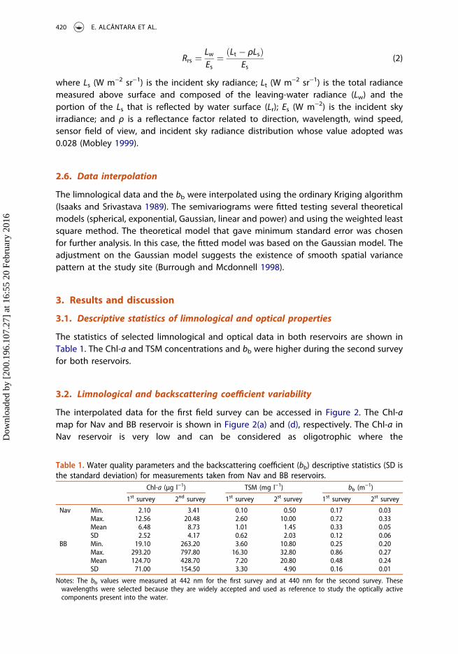
where Ls (W m−2 sr−1) is the incident sky radiance; Lt (W m−2 sr−1) is the total radiancemeasured above surface and composed of the leaving-water radiance (Lw) and theportion of the Ls that is reflected by water surface (Lr); Es (W m−2) is the incident skyirradiance; and ρ is a reflectance factor related to direction, wavelength, wind speed,sensor field of view, and incident sky radiance distribution whose value adopted was0.028 (Mobley 1999).

2.6. Data interpolation

The limnological data and the bb were interpolated using the ordinary Kriging algorithm(Isaaks and Srivastava 1989). The semivariograms were fitted testing several theoreticalmodels (spherical, exponential, Gaussian, linear and power) and using the weighted leastsquare method. The theoretical model that gave minimum standard error was chosenfor further analysis. In this case, the fitted model was based on the Gaussian model. Theadjustment on the Gaussian model suggests the existence of smooth spatial variancepattern at the study site (Burrough and Mcdonnell 1998).

3. Results and discussion

3.1. Descriptive statistics of limnological and optical properties

The statistics of selected limnological and optical data in both reservoirs are shown inTable 1. The Chl-a and TSM concentrations and bb were higher during the second surveyfor both reservoirs.

3.2. Limnological and backscattering coefficient variability

The interpolated data for the first field survey can be accessed in Figure 2. The Chl-amap for Nav and BB reservoir is shown in Figure 2(a) and (d), respectively. The Chl-a inNav reservoir is very low and can be considered as oligotrophic where the

Table 1. Water quality parameters and the backscattering coefficient (bb) descriptive statistics (SD isthe standard deviation) for measurements taken from Nav and BB reservoirs.

Chl-a (μg l−1) TSM (mg l−1) bb (m−1)

1st survey 2nd survey 1st survey 2st survey 1st survey 2st survey

Nav Min. 2.10 3.41 0.10 0.50 0.17 0.03Max. 12.56 20.48 2.60 10.00 0.72 0.33Mean 6.48 8.73 1.01 1.45 0.33 0.05SD 2.52 4.17 0.62 2.03 0.12 0.06

BB Min. 19.10 263.20 3.60 10.80 0.25 0.20Max. 293.20 797.80 16.30 32.80 0.86 0.27Mean 124.70 428.70 7.20 20.80 0.48 0.24SD 71.00 154.50 3.30 4.90 0.16 0.01

Notes: The bb values were measured at 442 nm for the first survey and at 440 nm for the second survey. Thesewavelengths were selected because they are widely accepted and used as reference to study the optically activecomponents present into the water.

420 E. ALCÂNTARA ET AL.

Dow

nloa

ded

by [

200.

196.

107.

27]

at 1

6:55

20

Febr

uary

201

6

concentrations are up to 3.24 μg l−1, and mesotrophic where the concentrations arefrom 3.24 to 11.03 μg l−1. The BB reservoir can be considered hypertrophic because theChl-a concentrations are higher than 69.05 μg l−1. This classification was based on theclassification adopted by the Environment Protection Agency in São Paulo State(CETESB, 2015).

The TSM concentrations were higher in the BB reservoir (Figure 2(c)) than in the Navreservoir (Figure 2(e)), as expected from Table 1. In Nav reservoir, the TSM concentra-tions were higher at the entrance of the reservoir where the water comes fromPromissão reservoir, decreasing downstream. For BB reservoir, the highest TSM concen-trations were found downstream near the dam including the small rivers in the south-east region of the reservoir and decreasing upstream towards the Piracicaba and TietêRivers.

The bb distribution for Nav and BB reservoirs was illustrated in Figure 2(c) and (f),respectively. In Nav reservoir, two spots were highlighted (see Figure 2 for location), thefirst (1) had the highest bb values and the spot (2) the lowest one. The correlationbetween TSM and Chl-a was 0.66 and the coefficient of determination R2 was 0.44,which means that about 44% of the TSM composition is dominated by Chl-a. In thiscase, the inorganic fraction of TSM is the main responsible for the bb distribution shownin Figure 2(c).

In BB reservoir, two spots were also identified (see Figure 2 for location): the first (3)shows a coincidence between high bb and TSM values and in spot (4) lowest bb values,which coincided with the lowest TSM concentration. However, there was a correlation of0.65 between the Chl-a and TSM, with a R2 of 0.43 and in the same fashion observed forNav reservoir, the main responsible for bb distribution was the inorganic fraction of TSM.In Figure 3, it is possible to see the bb vertical distribution for spots highlighted inFigure 2. Figure 3(a) and (b) is for Nav reservoir and Figure 3(c) and (d) is for BB reservoir.

Figure 2. Interpolated data using ordinary kriging: (a) chlorophyll-a, (b) total suspended matter, (c)backscattering coefficient at 442 nm for Nova Avanhandava reservoir and (d) chlorophyll-a, (e) totalsuspended matter, (f) backscattering coefficient at 442 nm for Barra Bonita reservoir. These datawere obtained during the first field survey. The numbers 1, 2, 3 and 4 highlighted in the figuresrepresent the location of high and low bb values in each reservoir.

REMOTE SENSING LETTERS 421

Dow

nloa

ded

by [

200.

196.

107.

27]

at 1

6:55

20

Febr

uary

201

6

Overall, spot 1 showed more variability of bb in depth than the others spots (Figure 3(a))and also showed that the highest bb values were observed at 442 nm and the lowest at700 nm.

For the second field survey, during the rainy season, the spatial patterns changed ifcompared with the first field survey during the dry season (Figure 4). Over again, theChl-a concentrations were higher for BB reservoir (Figure 4(a)) than for Nav reservoir(Figure 4(d)). Using the Chl-a concentrations, it is possible to classify some parts asmesotrophic and others as eutrophic for Nav reservoir and as eutrophic and hyper-trophic for BB reservoir. The TSM concentration was also higher in BB (Figure 4(b)) thanin Nav reservoir (Figure 4(e)). As same as for the first field survey, BB reservoir showedthe highest TSM concentrations near the dam. In Nav reservoir, the highest TSM con-centrations were located in south-west region of the reservoir.

The bb map for Nav reservoir matches with TSM concentration (Figure 4(c)), since thehighest bb (highlighted as 1) and the lowest (highlighted as 2) were coincident with thehigh and low TSM values. The highlighted regions 1 and 2 were the same highlighted forbb measured in the first field survey (see Figure 3(c)). The BB reservoir showed a morecomplex bb distribution (Figure 4(f)), but there were some coincidences with the bb mapfrom the first survey. In this case, the highest bb values (spot 4) were obtained in aregion with a high Chl-a concentration and the lowest bb values (spot 3) matched with aregion of low concentration.

Analysing the profiling bb data (Figure 5) by spots highlighted in Figure 4(c) and (f)we noticed that for Nav reservoir spot 1 (higher bb values) was higher only for wave-lengths at 412 and 440 nm. At longer wavelengths, the bb values decreased. In addition,we can see that there are slight changes with depth, and the only exception was at440 nm, with a little variability in the depth near 3 m; this indicated that the water

Figure 3. Vertical profiles of bb for Nova Avanhandava reservoir (a) and (b) represent the spots 1 and2, respectively, and for Barra Bonita reservoir (c) and (d) represent the spots 3 and 4, respectively.These data were obtained during the first field survey.

422 E. ALCÂNTARA ET AL.

Dow

nloa

ded

by [

200.

196.

107.

27]

at 1

6:55

20

Febr

uary

201

6

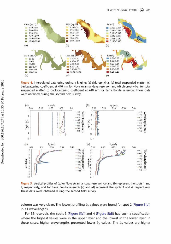
column was very clean. The lowest profiling bb values were found for spot 2 (Figure 5(b))in all wavelengths.

For BB reservoir, the spots 3 (Figure 5(c)) and 4 (Figure 5(d)) had such a stratificationwhere the highest values were in the upper layer and the lowest in the lower layer. Inthese cases, higher wavelengths presented lower bb values. The bb values are higher

Figure 4. Interpolated data using ordinary kriging: (a) chlorophyll-a, (b) total suspended matter, (c)backscattering coefficient at 440 nm for Nova Avanhandava reservoir and (d) chlorophyll-a, (e) totalsuspended matter, (f) backscattering coefficient at 440 nm for Barra Bonita reservoir. These datawere obtained during the second field survey.

Figure 5. Vertical profiles of bb for Nova Avanhandava reservoir (a) and (b) represent the spots 1 and2, respectively, and for Barra Bonita reservoir (c) and (d) represent the spots 3 and 4, respectively.These data were obtained during the second field survey.

REMOTE SENSING LETTERS 423

Dow

nloa

ded

by [

200.

196.

107.

27]

at 1

6:55

20

Febr

uary

201

6

than that observed for ocean waters in both reservoirs. Morel et al. (2007) studiedhyperoligotrophic waters in South Pacific and obtained bb values from 0.002 to 0.009(m−1) which are two orders of magnitude smaller than bb values found in Nav and BB.

The spatial and profiling patterns will modulate the spectral response that conse-quently will be captured by a remote sensor. The following section showed anddiscussed the spectral shape for those four spots highlighted in Figures 2 and 4.

3.3. Spectral reflectance

Since the Nav reservoir is a very clear water, with low Chl-a and TSM concentrations,then the main spectral behaviour showed higher reflectance at shorter wavelength andlower reflectance for longer wavelength (Figure 6(a) and (b)). These occur because therewas more penetration of electromagnetic radiation in the water column for shorterwavelengths, and since the concentrations are very low, the radiation penetrates deeper(Rijkeboer, Dekker, and Gons 1997).

Solar energy penetration largely determines the biological productivity of aquaticecosystems by controlling the heat budget, light availability for autotrophs at the baseof the food web (Belzile et al. 2004). Since the Nav reservoir has low TSM concentrations,the backscattering at longer wavelengths will be low as the reflectance. There was a shiftof the red wavelength towards longer wavelengths due to the increase in the TSMconcentration. This is especially true for the second field survey in Nav reservoir (Figure 6(b)) where the TSM concentration was 3.8 times higher than the TSM concentrationmeasured in the first field survey.

Figure 6. Rrs (sr−1) calculated for Nav and BB reservoirs, during the first (a, c) and second field survey

(b, d), respectively.

424 E. ALCÂNTARA ET AL.

Dow

nloa

ded

by [

200.

196.

107.

27]

at 1

6:55

20

Febr

uary

201

6

In BB reservoir, the absorption feature of the phycocyanin pigment at approximately620 nmwas associated with the presence of cyanobacteria in both field surveys (Figure 6(c)and (d)). In addition, there were a higher absorption at about 680 nm and a reflectance atapproximately 710 nm that can be associated with the Chl-a pigment (Watanabe et al.2015). Another reflection feature was observed at 810 nm associated with both Chl-a andorganic matter (Rundquist et al. 1996), which results from the low absorption of pure waterat this wavelength. The increase of reflectance in longer wavelength was indicative ofincreases in TSM concentration. The Chl-a concentration in BB reservoir during the secondsurvey was 2.8 times lower than in the first survey and this explained why the absorptionfor pigments was more evident during the second survey.

In the rainy season, the reflectance of both Nav and BB reservoirs was lower than thatmeasured during the dry season. The run-off generated due to the rain carried anamount of particles for the water surface, then the reflectance at shorter wavelengthsdecreased. The rain also helped in mixing and oxygenating the water column, whichprevented the phytoplankton blooms. During the dry season, the suspended matter wasnot on the surface anymore because they settled on the bottom. The reflectance atshorter wavelengths will increase, and due to the weather with hot air, lower windspeed the phytoplankton blooms took place.

4. Conclusion

The cascading reservoir configuration functions as a filter that improves the water quality.On the other hand, it contributes to decrease the optically active compounds concentra-tions and the values of bb. This filtration also alters the water reflectance. There was aseasonal influence on both limnological and optical data that can be explained by theinfluence of the rain (due to run-off). At the end of these cascading reservoirs, the spectrahad a shape of very clear water, without some characteristics of phytoplankton-laden water.

Disclosure statement

No potential conflict of interest was reported by the authors.

Funding

The authors thank São Paulo Research Foundation – FAPESP [Project number: 2012/19821-1] andNational Counsel of Technological and Scientific Development – CNPq [Projects numbers: 400881/2013-6 and 472131/2012-5] for financial support.

ORCID

Enner Alcântara http://orcid.org/0000-0002-7777-2119

REMOTE SENSING LETTERS 425

Dow

nloa

ded

by [

200.

196.

107.

27]

at 1

6:55

20

Febr

uary

201

6

References

APHA. 1998. Standard Methods for the Examination of Water and Wastewater. 20th ed. Washington,DC: American Public Health Association (APHA), American Water Works Association (AWWA),Water Environmental Federation (WEF).

Barbosa, F. A. R., J. Padisák, E. L. G. Espíndola, G. Borics, and O. Rocha. 1999. “The CascadingReservoir Continuum Concept (CRCC) and Its Application to the River Tietê-Basin, São Paulo State,Brazil.” In Theoretical Reservoir Ecology and Its Applications. International Institute of Ecology, eds.J. G. Tundisi, and M. Straskraba, 425–437. São Carlos: Academy of Sciences and BackhuysPublishers.

Belzile, C., W. F. Vincent, C. Howard-Williams, I. Hawes, M. R. James, M. Kumagai, and C. Roesler.2004. “Relationships between Spectral Optical Properties and Optically Active Substances in aClear Oligotrophic Lake.” Water Resources Research 40 (12): n/a–n/a. doi:10.1029/2004WR003090.

Burrough, P. A., and R. A. Mcdonnell. 1998. Principles of Geographical Information Systems, 333. NewYork: Oxford University Press.

CETESB (Companhia Ambiental do Estado de São Paulo). Águas superficiais. CETESB: São Paulo,Brasil. 2015. Accessed 23 April 2015. http://www.cetesb.sp.gov.br/agua/aguas-superficiais/35-publicacoes-/-relatorios

Golterman, H. L. 1975. Developments in Water Science 2. Physiological limnology: an approach tothe physiology of lake ecosystems. Amsterdam, Netherlands: Elsevier.

Isaaks, E. H., and M. R. Srivastava. 1989. An Introduction to Applied Geostatistics, 561 p. New York:Oxford University Press.

Kirk, J. T. O. 1994. Light and Photosynthesis in Aquatic Ecosystems. 2nd ed. Cambridge: CambridgeUniversity Press.

Loisel, H., X. Mériaux, J.-F. Berthon, and A. Poteau. 2007. “Investigation of the OpticalBackscattering to Scattering Ratio of Marine Particles in Relation to Their BiogeochemicalComposition in the Eastern English Channel and Southern North Sea.” Limnology andOceanography 52: 739–752. doi:10.4319/lo.2007.52.2.0739.

Maffione, R. A., and D. R. Dana. 1997. “Instruments and Methods for Measuring the Backward-Scattering Coefficient of Ocean Waters.” Applied Optics 36: 6057–6067. doi:10.1364/AO.36.006057.

Mobley, C. D. 1999. “Estimation of the Remote-Sensing Reflectance from Above-SurfaceMeasurements.” Applied Optics 38: 7442–7455. doi:10.1364/AO.38.007442.

Morel, A., B. Gentili, H. Claustre, M. Babin, A. Bricaud, J. Ras, and T. Fanny. 2007. “Optical Propertiesof the “Clearest” Natural Waters.” Limnology and Oceanography 52: 217–229. doi:10.4319/lo.2007.52.1.0217.

Padisák, J., F. A. R. Barbosa, G. Borbély, G. Borics, I. Chorus, E. L. G. Espíndola, R. Heinze, O. Rocha, A.K. Törökné, and G. Vasas. 2000. “Phytoplankton Composition, Biodiversity and a Pilot Survey ofToxic Cyanoprokaryotes in a Large Cascading Reservoir System (Tietê Basin, Brazil).” Verh.Internat. Verein. Limnol 27: 2734–2742.

Rijkeboer, M., A. G. Dekker, and H. J. Gons. 1997. “Subsurface Irradiance Reflectance Spectra ofInland Waters Differing in Morphometry and Hydrology.” Aquatic Ecology 31: 313–323.doi:10.1023/A:1009916501492.

Rundquist, D. C., L. Han, J. F. Schalles, and J. S. Peake. 1996. “Remote Measurement of AlgalChlorophyll in Surface Waters: The Case for the First Derivative of Reflectance near 690 Nm.”Photogrammetric Engineering & Remote Sensing 62: 195–200.

Soares, A., and A. A. Mozeto. 2006. “Water Quality in the Tietê River Reservoirs (Billings, BarraBonita, Bariri E Promissão, SP- Brazil) and Nutrient Fluxes across the Sediment-Water Interface(Barra Bonita).” Acta Limnologica Brasiliensia 18: 247–266.

Watanabe, F., E. H. Alcântara, T. Rodrigues, N. N. Imai, C. Barbosa, and L. Rotta. 2015. “Estimation ofChlorophyll-a Concentration and the Trophic State of the Barra Bonita Hydroelectric ReservoirUsing OLI/Landsat-8 Images.” International Journal of Environmental Research and Public Health12: 10391–10417. doi:10.3390/ijerph120910391.

WET Labs, Inc., 2013. Scattering Meter (ECO-BB9) User’s Guide. Revision L. http://www.wetlabs.com/manuals

426 E. ALCÂNTARA ET AL.

Dow

nloa

ded

by [

200.

196.

107.

27]

at 1

6:55

20

Febr

uary

201

6