Reserve Requirements and Optimal Chinese Stabilization … · RESERVE REQUIREMENTS AND OPTIMAL...
37
FEDERAL RESERVE BANK OF SAN FRANCISCO WORKING PAPER SERIES Reserve Requirements and Optimal Chinese Stabilization Policy Chun Chang Shanghai Advanced Institute of Finance Shanghai Jiao Tong University Zheng Liu and Mark M. Spiegel Federal Reserve Bank of San Francisco Jingyi Zhang Shanghai Advanced Institute of Finance Shanghai Jiao Tong University March 2018 Working Paper 2016-10 http://www.frbsf.org/economic-research/publications/working-papers/2016/10/ Suggested citation: Chang, Chun, Zheng Liu, Mark M. Spiegel, Jingyi Zhang. 2018. “Reserve Requirements and Optimal Chinese Stabilization Policy.” Federal Reserve Bank of San Francisco Working Paper 2016-10. https://doi.org/10.24148/wp2016-10 The views in this paper are solely the responsibility of the authors and should not be interpreted as reflecting the views of the Federal Reserve Bank of San Francisco or the Board of Governors of the Federal Reserve System. This paper was produced under the auspices of the Center for Pacific Basin Studies within the Economic Research Department of the Federal Reserve Bank of San Francisco.
Transcript of Reserve Requirements and Optimal Chinese Stabilization … · RESERVE REQUIREMENTS AND OPTIMAL...

FEDERAL RESERVE BANK OF SAN FRANCISCO
WORKING PAPER SERIES
Reserve Requirements and Optimal Chinese Stabilization Policy
Chun Chang Shanghai Advanced Institute of Finance
Shanghai Jiao Tong University
Zheng Liu and Mark M. Spiegel Federal Reserve Bank of San Francisco
Jingyi Zhang
Shanghai Advanced Institute of Finance Shanghai Jiao Tong University
March 2018
Working Paper 2016-10
http://www.frbsf.org/economic-research/publications/working-papers/2016/10/
Suggested citation:
Chang, Chun, Zheng Liu, Mark M. Spiegel, Jingyi Zhang. 2018. “Reserve Requirements and Optimal Chinese Stabilization Policy.” Federal Reserve Bank of San Francisco Working Paper 2016-10. https://doi.org/10.24148/wp2016-10 The views in this paper are solely the responsibility of the authors and should not be interpreted as reflecting the views of the Federal Reserve Bank of San Francisco or the Board of Governors of the Federal Reserve System. This paper was produced under the auspices of the Center for Pacific Basin Studies within the Economic Research Department of the Federal Reserve Bank of San Francisco.

RESERVE REQUIREMENTS AND OPTIMAL CHINESE STABILIZATIONPOLICY
CHUN CHANG, ZHENG LIU, MARK M. SPIEGEL, JINGYI ZHANG
Abstract. We build a two-sector DSGE model to study reserve requirement adjustments,
a frequently-used policy tool for macro-stabilization in China. State-owned enterprises
(SOEs) are financed by government-guaranteed bank loans, which are subject to reserve
requirements, while private firms rely on unregulated off-balance sheet financing. Increasing
reserve requirements reallocates resources to more productive private firms, raising aggregate
productivity, but also raises the incidence of SOE bankruptcy. Optimal reserve requirement
adjustments are complementary to money supply adjustments for improving macroeconomic
stability and welfare. However, welfare gains are greater under sector-specific productivity
shocks, which call for resource reallocation, than under aggregate productivity shocks.
Date: March 19, 2018.
Key words and phrases. Reserve requirements, Chinese monetary policy, off-balance sheet loans, financial
accelerator, reallocation and productivity.
JEL classification: E44, E52, G28.
Chang: Shanghai Advanced Institute of Finance, Shanghai Jiao Tong University; Email:
[email protected]. Liu: Federal Reserve Bank of San Francisco; Email: [email protected]. Spiegel:
Federal Reserve Bank of San Francisco; Email: [email protected]. Zhang: Shanghai Advanced In-
stitute of Finance, Shanghai Jiao Tong University; Email: [email protected]. We are grateful to
the Editors Urban Jermann and Vivian Yue and an anonymous referee for insightful comments that helped
improve the paper. For helpful discussions, we thank Kaiji Chen, David Cook, Jonathan Ostry, Haibing
Shu, Michael Zheng Song, Jian Wang, Shang-Jin Wei, Tao Zha, Feng Zhu, Xiaodong Zhu, and seminar par-
ticipants at the 2017 Asian Meeting of the Econometric Society, the Federal Reserve Bank of San Francisco,
Fudan University, the IMF, the NBER Chinese Economy Meeting, Conference on “Business Cycles, Finan-
cial markets, and Monetary Policy” in Beijing, the University of Toronto and Bank of Canada Conference on
the Chinese Economy, the Central Bank of Chile Conference on the Chinese Economy, Chinese University
of Hong Kong, Hong Kong University of Science and Technology, George Washington University, Zhejiang
University, and the HKIMR. We also thank Andrew Tai for research assistance and Anita Todd for editorial
assistance. The research is supported by the National Natural Science Foundation of China Project Number
71633003. The views expressed in this paper are those of the authors and do not necessarily reflect the views
of the Federal Reserve Bank of San Francisco or the Federal Reserve System.1

RESERVE REQUIREMENTS AND OPTIMAL CHINESE STABILIZATION POLICY 2
I. Introduction
China’s central bank, the People’s Bank of China (PBOC), frequently uses reserve re-
quirements (RR) as a policy instrument for macroeconomic stabilization. Since 2006, the
PBOC has adjusted the required reserve ratio at least 40 times. These changes have also
been substantial. For example, during the tightening cycle from 2006 to 2011, the required
reserve ratio increased from 8.5 percent to 21.5 percent (see Figure 1).
While many emerging market economies use RR as a policy instrument for stabilizing do-
mestic activity (Federico, Vegh, and Vuletin, 2014), RR adjustments are also used to address
external imbalances. For the bulk of countries with open capital accounts, adjusting RR can
mitigate potentially disruptive capital flows (Montoro and Moreno, 2011). In the specific
case of China, the government has maintained tight controls over both its capital account
and the RMB exchange rate. This policy regime allows for substantive and persistent devi-
ations from the interest rate parity. Chang, Liu, and Spiegel (2015) argue that quantitative
easing in the advanced economies during the global financial crisis raised the sterilization
costs for the PBOC because the interest rates on U.S. Treasuries have fallen substantially
relative to Chinas interest rates (such as the SHIBOR). Raising reserve requirements helped
to mitigate the PBOCs need to engage in costly sterilization and also reduce the cost of
achieving, for example, an exchange rate target or some other macroeconomic policy goals
under Chinas tightly controlled capital account regime.1
In this paper, we argue that RR adjustments also have re-allocative consequences under
China’s existing financial system. The Chinese government provides explicit or implicit
guarantees for loans to SOEs (Song, Storesletten, and Zilibotti, 2011). As a result, SOEs
enjoy an advantage in raising capital through formal bank borrowing over private firms
(POEs). In contrast, POEs, particularly small and medium-sized private firms, raise capital
mainly through off-balance sheet lending by commercial banks or by borrowing from informal
financial intermediaries or “shadow banks” (Lu, Guo, Kao, and Fung, 2015).
These different borrowing channels face different regulatory conditions. On-balance sheet
bank loans to SOEs are subject to RR regulations, while off-balance sheet banking activities
are not. As a result, raising RR inhibits SOE financing and encourages the reallocation of
capital from the SOE sector to the POE sector. Moreover, since private firms in China are
1Cun and Li (2017) argue that China’s sterilized intervention results in an unintended expansion of bank
lending, limiting its effectiveness as a stabilization tool.

RESERVE REQUIREMENTS AND OPTIMAL CHINESE STABILIZATION POLICY 3
on average more productive than SOEs (Hsieh and Klenow, 2009; Hsieh and Song, 2015),
holding all else equal, this reallocation may raise aggregate productivity.2
We develop a DSGE model to evaluate the implications of RR adjustments for reallocation
and macroeconomic stabilization. In the model, intermediate goods are produced by firms
in two sectors—an SOE sector and a POE sector—using the same production technology,
but with POEs having higher average productivity. The intermediate goods produced by
the two sectors are imperfect substitutes. Final goods are produced using a composite of the
sectoral intermediate goods and also capital and labor as inputs.
To incorporate financial frictions, we build on the framework of Bernanke, Gertler, and
Gilchrist (1999) (BGG). Firms in each sector face aggregate and idiosyncratic productivity
shocks. They need to finance working capital with both internal net worth and external
debt. As in BGG, there is a threshold level of idiosyncratic productivity, above which
firms repay the loans at the contractual interest rate and earn nonnegative profits. Firms
with productivity below the threshold level, however, will default, resulting in costly state
verification and liquidation.
To illustrate the allocative implications of RR adjustments in China, we extend the BGG
framework in several dimensions. First, we assume that bank lending activity is segmented.
On-balance sheet loans are provided to SOE firms only, while POE firms can obtain funding
only through banks’ off-balance sheet activity. This strict separation is a simplification.
In reality, both types of firms can obtain funding through both on- and off- balance sheet
channels, and SOEs even engage in some lending to POEs. Still, SOEs do receive the
substantive majority of on-balance sheet lending, while the POE sector primarily depends
on off-balance sheet borrowing from commercial banks and shadow banks (Elliott, Kroeber,
and Qiao, 2015).3
Second, the government provides guarantees for SOE debt, covering bank losses in the
event of an SOE default. This guarantee leads banks to lend at a risk-free interest rate to
SOEs, since default losses including deadweight liquidation costs are borne by the government—
and ultimately, by the households, since the government needs to finance the SOE bailout
2Although SOE productivity is lower on average, firm-level evidence indicates substantial within-sector
heterogeneity in productivity. For example, Brandt (2015) shows that both SOEs and POEs have lower
productivity in SOE-dominant industries than firms in industries with less SOE presence.3Chang, Chen, Waggoner, and Zha (2015) provide evidence that China’s credit policy favors capital-
intensive (or heavy) industries at the expense of labor-intensive (or light) industries. While some heavy
industry firms are not state-owned, Chang et al. (2015) find that the share of SOEs in capital-intensive
industries has increased steadily since the late 1990s reforms. One could more generally interpret our strict
financing dichotomy as illustrative of the implications of preferential treatment by the Chinese government
across firm types.

RESERVE REQUIREMENTS AND OPTIMAL CHINESE STABILIZATION POLICY 4
costs through lump-sum taxes. Off-balance sheet loans to private firms are not guaranteed,
and the financial frictions facing POEs mimic those in the standard BGG environment. In
particular, POE loan rates compensate for expected losses under default. In tandem, these
assumptions imply that the BGG financial accelerator mechanism is active for the POE sec-
tor, but muted for the SOE sector. This leaves POE firms more sensitive to macroeconomic
shocks. Furthermore, government guarantees on SOE loans drive a wedge between the rela-
tive price of SOE goods and SOE productivity, leading to potentially inefficient fluctuations
in SOE relative prices, especially when the economy is buffeted by sector-specific shocks.
Third, RR policy raises the costs of banks’ on-balance sheet activity since banks do not
earn interest on reserves in our model. Thus, RR policy drives a wedge between the deposit
interest rate and the lending rate.4
Our model implies that raising RR discourages on-balance sheet lending activity and
reallocates capital from SOEs to POEs. This reallocation mechanism is consistent with
empirical evidence from Chinese data, as we show in Section II below. This transmission
mechanism differs from conventional monetary policy, which is conducted in China through
money supply adjustments (Chen, Ren, and Zha, 2017; Chen, Higgins, Waggoner, and Zha,
2017). While changes in money supply tend to stimulate or contract activities in both the
SOE and the POE sectors, an adjustment in RR has different impacts on the two sectors and
helps mitigate inefficient relative-price fluctuations. Thus, adjusting RR can be an important
complementary policy tool for stabilizing China’s macroeconomic fluctuations.
We calibrate our model to illustrate the implications of RR adjustments. We first demon-
strate that, in the steady-state equilibrium in our model, adjustments in RR incur a tradeoff.
An increase in the steady-state RR ratio improves aggregate total factor productivity (TFP)
by reallocating resources toward the more productive POE sector, but it also raises the
incidence of SOE bankruptcies and thus the social costs of SOE bailouts.
We then examine the implications of a simple RR rule and a money growth rule for
macroeconomic stability and social welfare under either aggregate or sector-specific produc-
tivity shocks.5 Under these simple rules, the policy instrument (the RR ratio or the money
growth rate) reacts to fluctuations in inflation and the real GDP growth. We then search
for optimal rule coefficients that maximize the representative household’s welfare.6
4We set the interest rate on reserves to zero for simplicity. The actual current interest rate paid on required
reserves in China is 1.62%, far below the 2.74% one- year government bond rate or the 3.26% PBOC bills
rate, implying that RR do act as a tax on banking activity.5An example of such sector-specific shocks in China is the large-scale SOE restructuring in the late 1990s,
which led to significant improvement in the relative productivity of the SOEs (Hsieh and Song, 2015).6We restrict the planner’s problem to simple rules because the model proved too complex to solve for the
full Ramsey equilibrium.

RESERVE REQUIREMENTS AND OPTIMAL CHINESE STABILIZATION POLICY 5
We evaluate four alternative policy rules. We first consider a benchmark economy in
which the monetary authority maintains a constant RR ratio and adjusts the money growth
in response to fluctuations in inflation and output growth, with the money growth rule
parameters calibrated based on the empirical evidence documented by Chen et al. (2017).
We then examine optimal simple rules, with the parameters in either of these two policy
rules chosen optimally to maximize social welfare. Finally, we allow the parameters in both
policy rules to be adjusted optimally.
We find that individually optimal RR rule and optimal money growth rule both improve
welfare relative to the benchmark policy. Adjusting both instruments optimally yields further
welfare gains, suggesting that the two policy instruments are complementary. Furthermore,
the magnitudes of the welfare gains obtained from adjusting both reserve requirements and
the money growth rate relative to those obtained from optimally adjusting the money growth
rate alone depend on the source of the shocks. Gains are greater under situations that call
for reallocations of resources across sectors, such as a sector-specific productivity shock, than
under aggregate TFP shocks.7
Our paper is related to the recent literature on shadow banking in China. For example,
Hachem and Song (2015), Chen, Ren, and Zha (2016) Chen et al. (2017), and Wang, Wang,
Wang, and Zhou (2016) discuss the underlying factors that drove the dramatic expansion
in shadow banking activity in China between 2009 and 2013. Over that period, China’s
shadow bank lending increased by over 30 percent per year, largely financed by off-balance
sheet commercial bank activity in the forms of wealth management products and entrusted
loans. Funke, Mihaylovski, and Zhu (2015) study the role of shadow banks for China’s
monetary policy transmission.
Our work is also related to the earlier literature on sectoral preferences of China’s macroe-
conomic policy. Brandt and Zhu (2000) examine the implications of commitment by the
Chinese government for maintaining employment in its less efficient state sector. They find
that the cost of fulfilling this commitment has implications for monetary policy and inflation.
Song et al. (2011) examine China’s transition dynamics in a two-period overlapping gener-
ations model with SOEs and POEs. As in our paper, these authors postulate that SOEs
have lower productivity, but enjoy superior access to bank credit. Their model’s transition
dynamics explain some puzzling characteristics of the Chinese economy, such as high growth
being accompanied by high saving rates.
7In an earlier working paper version, we considered an interest rate rule instead of the money growth rule
as a benchmark policy regime and obtained qualitatively similar results (see Chang, Liu, Spiegel, and Zhang
(2017)).

RESERVE REQUIREMENTS AND OPTIMAL CHINESE STABILIZATION POLICY 6
Our model differs from the earlier literature in three dimensions. First, we investigate
an infinite-horizon DSGE model, which accommodates the study of both the steady-state
equilibrium and business cycle dynamics. Second, we model financial frictions in the spirit
of Bernanke et al. (1999) (BGG). Third, we study the implications of RR policy relative to
the conventional monetary policy in an environment with nominal rigidities and financial
frictions. In this second-best environment, we find that RR policy is useful for not just
steady-state reallocation, but also for business cycle stabilization.
II. The reallocation effects of reserve requirement policy: Some evidence
Our model implies that an increase in reserve requirements reallocates capital from SOEs
to POEs because it raises the relative cost of on-balance sheet banking activity. In this sec-
tion, we demonstrate that this reallocation mechanism is consistent with empirical evidence
at both the micro level and the macro level.
II.1. Firm-level evidence. We first present some firm-level evidence based on China’s
equity market data. Our model suggests that an increase in RR directly raises the cost of
external financing for SOEs, since they borrow primarily through on-balance sheet channels.
In contrast, increases in RR should have a smaller adverse impact on POE activity, since
POEs borrow mainly through off-balance sheet activity.
To evaluate the existence of an asymmetric effect of RR changes, we conduct an event
study to estimate the announcement effects of changes in RR policy on the equity values of
SOEs relative to those of POEs. We use panel data to estimate the empirical specification
H∑h=−H
Rej,t+h = a0 + a1∆RRt−1 + a2SOEjt ×∆RRt−1 + a3SOEjt + bZjt + εjt. (1)
where the left-hand-side variable Rejt denotes risk-adjusted excess returns for firm j in period
t, defined as Rejt = Rjt − βjRmt, where Rjt denotes the firm’s stock return, Rmt the market
return, and βj the firm’s “market beta” (i.e.. the estimated slope coefficient in the regression
of the firm’s return on a constant and the market return). The dependent variable in our
empirical specification is the cumulative risk-adjusted excess returns within the window of
time from H days before to H days after a given date t. The regressors include ∆RRt−1,
which denotes changes in RR; SOEjt, which is a 0-1 dummy variable indicating whether the
firm is an SOE;8 interactions between changes in RR and the SOE dummy; Zjt, which is
a vector of control variables, including firm size, book-to-market value ratio, industry fixed
8We identify SOEs as firms that are is directly controlled by the state or has the state as its majority
shareholder.

RESERVE REQUIREMENTS AND OPTIMAL CHINESE STABILIZATION POLICY 7
effects, and year fixed effects. The term εjt denotes regression errors, assumed to be well
behaved.
The parameter of interest is a2, the coefficient on the interaction term. It captures the
additional sensitivity of SOE stock returns to the announcements of changes in RR policy.
In particular, if an increase in RR reduces the relative SOE stock returns, we should observe
that a2 < 0.
We estimate the model in equation (1) using daily data from non-financial firms listed in
the Shanghai and Shenzhen stock exchanges for the period from 2005 to 2015. Under China’s
current regulations, a change in RR policy is not to be signaled or leaked before the actual
announcement. Thus, within a relatively short window of time around the announcement
date, changes in RR policy are likely to contain some surprise component that can potentially
affect stock returns.
Table 1 shows the estimation results for three different window lengths around the RR
change announcements: the same day of the announcement (H = 0), a three-day window
(H = 1), and a five-day window (H = 2). The estimated value of a2 is negative and
statistically significant at the 99% level for all 3 different window lengths. The negative
estimates of a2 are also economically significant. For example, on the same day of the
RR policy change, our point estimate indicates that a one percentage point increase in the
required reserve ratio would reduce the daily stock return of an average SOE firm relative
to a non-SOE firm by about 0.12%. This corresponds to a monthly reduction in the relative
SOE stock returns of about 2.43%, or an annualized reduction of about 33%.9 Our point
estimates for the three-day and five-day windows are even larger.
There is reason to believe that this difference in sensitivity is predominantly driven by
the latter portion of our sample. In China, the demand for off-balance sheet loans expanded
rapidly following the large fiscal stimulus plan that was announced in November 2008 and
implemented in 2009-2010. Thus, we expect a stronger reallocation effect of changes in RR
in the sample after the fiscal stimulus plan was adopted.10
To investigate this possibility, we split our sample into pre- (2005-2008) and post- (2009-
2015) stimulus periods. Our results are shown in Table 2. The estimates of a2 are not
significantly different from zero in the pre-stimulus period, but become significantly nega-
tive in the post-stimulus sample. Moreover, the value of a2 estimated in the post-stimulus
9This calculation is based on 20 trading days per month. The PBOC typically changes the required
reserve ratio by 50 basis points, although on some occasions, the size of the change can be as large as 100
basis points.10Cong and Ponticelli (2017) find evidence that China’s large-scale fiscal stimulus exacerbated the dis-
crepancies in access to credit between SOEs and POEs, since new credit under the stimulus was primarily
allocated toward SOEs.

RESERVE REQUIREMENTS AND OPTIMAL CHINESE STABILIZATION POLICY 8
sample is about twice as large (in absolute terms) as our full-sample estimate shown in Ta-
ble 1.11 Our results therefore indicate that SOE equity values were particularly sensitive to
announcements of RR policy changes during the post-stimulus period, when shadow banking
activity was expanding rapidly.
II.2. Some VAR evidence. We next present macro evidence that supports the reallocation
mechanism of RR adjustments featured in our DSGE model. In particular, this mechanism
implies that an increase in RR should raise the borrowing costs for SOEs, reduce the amount
of loans made to SOEs, and lower SOE investment.
Although changes in RR directly affect bank lending rates, the extent to which such
changes can affect SOE borrowing and investment remains unclear. With soft budget con-
straints and monopoly power, SOE activity may be insensitive to changes in market interest
rates. We examine the quantitative macro impact of changes in RR on SOE activity using
a Bayesian vector-autogression (BVAR) framework.
The BVAR specification that we consider includes 4 variables: new loans to the heavy
industry sector (which is a good proxy for SOE loans in light of the evidence in Chang et al.
(2015)), the share of SOE investment in total business investment, the one-year benchmark
bank lending rate, and the required reserve ratio (RRR). All data are taken from Chang
et al. (2015), with a sample range from 2003:Q1 to 2015:Q4. In the baseline BVAR model,
we order RRR the last, reflecting our Cholesky identification assumption that RR policy
responds to shocks to heavy industry loans, SOE investment shares, and the lending rate in
the impact period, but those macro variables do not respond to shocks to RRR on impact.12
The BVAR model is estimated with four quarterly lags and with the Sims-Zha priors.
Figure 2 shows the impulse responses to a one standard deviation positive shock to RR,
estimated from the BVAR model in our sample. The shock raises RR, pushes up the lending
rate, reduces new loans to the heavy industry sector (or SOEs), and reduces the SOE in-
vestment share. These macro responses are all statistically significant at the 68% confidence
level.
Our macro evidence based on the estimated BVAR model, along with the firm-level evi-
dence based on the equity market data, lend empirical support to our model’s main mecha-
nism. In particular, consistent with our model’s predictions, an increase in reserve require-
ments raises the cost of on-balance sheet loans, which disproportionately weighs on SOE
borrowings and reduces the SOE investment share.
11To conserve space, we only display estimation results for the one- and three-day windows. Results for
the five-day window are similar.12We obtained similar qualitative results if RR is ordered the first.

RESERVE REQUIREMENTS AND OPTIMAL CHINESE STABILIZATION POLICY 9
III. The model
The economy is populated by a continuum of infinitely lived households. The representa-
tive household consumes a basket of differentiated goods purchased from retailers. Retailers
produce differentiated goods using a homogeneous wholesale good as the only input. The
wholesale good is itself a composite of intermediate goods produced by two types of firms:
SOEs and POEs. With the exception of SOEs having lower average productivity, the two
types of firms have identical ex-ante production technologies.
Firms face working capital constraints. Each firm finances wages and rental payments
using both internal net worth and external debt. Following Bernanke et al. (1999), we
assume that external financing is subject to a costly state verification problem. In particular,
only firms can costlessly observe their own idiosyncratic productivity shocks. Firms with
sufficiently low productivity relative to their nominal debt obligations will default and be
liquidated. Lenders suffer a liquidation cost when taking over the project to seize available
revenue.
We generalize the BGG framework to a two-sector environment with SOEs and POEs that
have access to different sources of external financing. We assume that SOEs only borrow
through formal on-balance-sheet loans. As is effectively the case in China, we also assume
that these loans are backed by government guarantees. In contrast, POEs only borrow
through off-balance-sheet loans, which are neither regulated nor backed by the government.
While banks face no default risk on the guaranteed loans to SOEs, they face expected default
costs for off-balance sheet loans extended to POEs, as in the BGG framework.13
We assume that intermediate goods produced by SOEs and by POEs are imperfect sub-
stitutes, to ensure positive demand for the lower productivity SOE product. As we show
below, financial frictions stemming from government guarantees on SOE loans drive a wedge
between the relative price and relative productivity of the SOE sector, causing inefficiencies
in resource allocation in both the steady state and over the business cycle.14
III.1. Households. There is a continuum of infinitely lived and identical households with
unit mass. The representative household has preferences represented by the expected utility
13Our framework is a simplification that allow for solution of the model. Off-balance sheet lending in
China is more diverse and complex, including private loans and corporate bonds. Moreover, large and
profitable Chinese private firms typically also have no difficulties accessing bank loans, but rely more on
equity and bond markets for capital. In the end, consistent with our assumptions, the bulk of on-balance
sheet commercial bank lending goes to SOEs.14In what follows, we focus on describing the main features of the model and we relegate detailed deriva-
tions of the equilibrium conditions in an appendix available at the web site http://www.frbsf.org/
economic-research/files/wp2016-10_appendix.pdf

RESERVE REQUIREMENTS AND OPTIMAL CHINESE STABILIZATION POLICY 10
function
U = E∞∑t=0
βt[ln(Ct)−Ψ
H1+ηt
1 + η+ Ψm ln
(Mt
Pt
)], (2)
where E is an expectations operator, Ct denotes consumption, Ht denotes labor hours, and
Mt denotes cash holdings. The parameter β ∈ (0, 1) is a subjective discount factor, η > 0 is
the inverse Frisch elasticity of labor supply, and Ψ > 0 and Ψm > 0 are the relative weights
on the disutility of working and the utility of holdings of real cash balances.
The household faces the sequence of budget constraints
Ct + It +Mt
Pt+Dt
Pt= wtHt + rktKt−1 +
Mt−1
Pt+Rt−1
Dt−1
Pt+ Tt, (3)
where It denotes capital investment, Dt denotes deposits in banks, wt denotes the real wage
rate, rkt denotes the real rent rate on capital, Kt−1 denotes the level of the capital stock
at the beginning of period t, Rt−1 is the gross nominal interest rate on household savings
determined from information available in period t − 1, Pt denotes the price level, and Tt
denotes the lump-sum transfers (or taxes if negative) from the government and earnings
received from firms based on the household’s ownership share.
The capital stock evolves according to the law of motion
Kt = (1− δ)Kt−1 +
[1− Ωk
2
(ItIt−1− gI
)2]It, (4)
where we have assumed that changes in investment incur an adjustment cost, the scale of
which is measured by the parameter Ωk > 0. The constant gI denotes the steady-state
growth rate of investment.
The household chooses Ct, Ht, Dt, Mt, It, and Kt to maximize (2), subject to the con-
straints (3) and (4).
III.2. The retail sector and price setting. There is a continuum of retailers, each pro-
ducing a differentiated retail product indexed by z ∈ [0, 1]. The retail goods are produced
using a homogeneous wholesale good, with a constant-returns technology. Retailers are price
takers in the input market and face monopolistic competition in the product markets. Retail
price adjustments are subject to a quadratic cost, as in Rotemberg (1982).
The production function of retail good of type z is given by
Yt(z) = Γt(z), (5)
where Yt(z) denotes the output of the retail good and Γt(z) the intermediate input.

RESERVE REQUIREMENTS AND OPTIMAL CHINESE STABILIZATION POLICY 11
The final good for consumption and investment (denoted by Y ft ) is a Dixit-Stiglitz com-
posite of all retail products given by
Y ft =
[∫ 1
0
Yt(z)ε−1ε dz
] εε−1
, (6)
where ε > 1 denotes the elasticity of substitution between retail goods.
The optimizing decisions of the final good producer lead to a downward-sloping demand
schedule for each retail product z:
Y dt (z) =
(Pt(z)
Pt
)−εY ft , (7)
where Pt(z) denotes the price of retail product z.
The zero-profit condition for the final good producer implies that the price level Pt is
related to retail prices by
Pt =
[∫ 1
0
Pt(z)(1−ε)dz
]1/(1−ε). (8)
Each retailer takes as given the demand schedule (7) and the price level Pt, and sets a
price Pt(z) to maximize profits. Price adjustments are costly, with the cost function given
by
Ωp
2
(Pt(z)
πPt−1(z)− 1
)2
Ct,
where Ωp measures the size of the adjustment cost and π is the steady-state inflation rate.
Retailer z chooses Pt(z) to maximize its expected discounted profit
Et
∞∑i=0
βiΛt+i
[(Pt+i(z)
Pt+i− pw,t+i
)Y dt+i(z)− Ωp
2
(Pt+i(z)
πPt+i−1(z)− 1
)2
Ct+i
], (9)
where pwt is the relative price of the wholesale good (expressed in consumption units) and
Y dt+i(z) is given by the demand schedule (7).
We focus on a symmetric equilibrium in which Pt(z) = Pt for all z. The optimal price-
setting decision implies the Phillips curve relation
pwt =ε− 1
ε+
Ωp
ε
1
Yt
[(πtπ− 1) πtπCt − βEt
Λt+1
Λt
(πt+1
π− 1) πt+1
πCt+1
]. (10)
In the special case with no nominal rigidities (i.e., with Ωp = 0), the retail good price would
be a constant markup over the marginal cost, so that the relative price of wholesale goods
would be the inverse of the steady-state markup. In general, in the presence of nominal
rigidities, the Phillips curve in Equation (10) implies that the current-period inflation πt
increases with both the real marginal cost and the expected next-period inflation rate.

RESERVE REQUIREMENTS AND OPTIMAL CHINESE STABILIZATION POLICY 12
III.3. The wholesale sector. Wholesale goods are a composite of intermediate goods from
both sectors. Denote by Yst and Ypt the products produced by SOE firms and POE firms,
respectively. The quantity of the wholesale good Γt is given by
Γt =(φY
σ−1σ
st + (1− φ)Yσ−1σ
pt
) σσ−1
, (11)
where φ ∈ (0, 1) measures the share of SOE goods and σ > 0 is the elasticity of sbustitution
between goods produced by the two sectors.
Denote by pst and ppt the relative price of SOE products and POE products, respectively,
expressed in final consumption units. Cost-minimization implies
Yst = φσ(pstpwt
)−σΓt, Ypt = (1− φ)σ
(pptpwt
)−σΓt. (12)
Zero-profits in the wholesale sector imply that
pwt =(φσp1−σst + (1− φ)σp1−σst
) 11−σ . (13)
III.4. The intermediate goods sectors. We now present the environment in the SOE and
POE intermediate goods sectors. We focus on a representative firm in each sector j ∈ s, p.A firm in sector j produces a homogeneous intermediate good Yjt using capital Kjt and
two types of labor inputs— household labor Hjt and entrepreneurial labor Hejt, with the
production function
Yjt = Ajtωjt(Kjt)1−α [(He
jt)1−θHθ
jt
]α, (14)
where Ajt denotes a common productivity shock to all firms in sector j, and the parameters
α ∈ (0, 1) and θ ∈ (0, 1) are input elasticities in the production function. The term ωjt is an
idiosyncratic productivity shock at the firm level, and it is an i.i.d. process across firms and
time, drawn from the distribution F (·) with a nonnegative support. We assume that the
idiosyncratic productivity shocks are drawn from a Pareto distribution with the cumulative
density function F (ω) = 1 − (ωmω
)k over the range [ωm,∞), where ωm > 0 is the scale
parameter and k is the shape parameter. Here, we implicitly assume that the idiosyncratic
productivities in both sectors are drawn from the same distribution F (·).Productivity Ajt contains a common deterministic trend gt and a sector-specific stationary
component Amjt so that Ajt = gtAmjt . The stationary component Amjt follows the stochastic
process
lnAmjt = (1− ρj) ln Aj + ρj lnAmj,t−1 + εjt, (15)
where Aj is the steady-state level of Amj , ρj ∈ (−1, 1) is a persistence parameter, and the
term εjt is an i.i.d. innovation drawn from a log-normal distribution N(0, σj).
Firms face working capital constraints. In particular, they need to pay wage bills and
capital rents before production takes place. Firms finance working capital payments through

RESERVE REQUIREMENTS AND OPTIMAL CHINESE STABILIZATION POLICY 13
both their beginning-of-period net worth Nj,t−1 and external debt Bjt. The working capital
constraint for a firm in sector j ∈ s, p is given by
Nj,t−1 +Bjt
Pt= wtHjt + wejtH
ejt + rktKjt. (16)
where wejt denotes the real wage rate of managerial labor in sector j.
Under constant returns to scale, cost-minimizing factor demand implies that a firm’s
revenue is a linear function of its net worth, as in Bernanke et al. (1999).
III.5. Financial intermediaries and debt contracts. Financial intermediation takes
place through a continuum of competitive representative commercial banks. At the be-
ginning of each period t, the representative commercial bank receives deposits Dt from the
household at interest rate Rt. The bank makes on-balance-sheet loans Bst to SOE firms,
and off-balance-sheet loans Bpt to POE firms. On-balance sheet loans are subject to reserve
requirements, whereas off-balance sheet loans are not.
In each period, a fraction of firms in both sectors with sufficiently low levels of realized
idiosyncratic productivity choose to default on their loan repayments. Off-balance sheet
loans do carry default risk. This results in a credit spread on off-balance sheet loans, as in
BGG. However, SOE loan losses are covered by the government, eliminating bank default
risk.
Given the government guarantees, SOEs face a risk-free loan rate of Rst. However, reserve
requirements drive a wedge between the loan and deposit interest rates so that
(Rst − 1)(1− τt) = (Rt − 1), (17)
where τt is the required reserve ratio .
Off-balance sheet lending to POEs is not subject to reserve requirements. Bank funding
costs on these loans are therefore equal to Rpt = Rt. Banks charge a higher contractual
interest rate Zjt (j = s, p) on all loans ex-ante to cover expected monitoring and liquidation
costs. Firms with realized productivity below a cut-off level ωjt will choose to default, where
ωjt satisfies
ωjt ≡ZjtBjt
Ajt(Nj,t−1 +Bjt), (18)
where the term Ajt, which represents the rate of return on the firm’s investment financed by
external debt and internal funds, is given by
Ajt = pjtAjt
(1− αrkt
)1−α[(
α(1− θ)wejt
)1−θ (αθ
wt
)θ]α. (19)
If a firm defaults, the bank pays the liquidation cost and obtains the firm’s generated
revenue. In the process, a fraction mj of output is lost. Furthermore, the government is

RESERVE REQUIREMENTS AND OPTIMAL CHINESE STABILIZATION POLICY 14
assumed to cover a fraction lj of the loan losses financed by lump-sum taxes collected from
the households, where ls = 1 and lp = 0, i.e. the government covers losses on SOE defaults
but not on POE defaults.
We now describe the optimal contract. Denote by f(ωjt) and g(ωjt) the share of sector-j
income that goes to the borrower and the lender, respectively. The optimal contract is a pair
(ωjt, Bjt) chosen at the beginning of period t to maximize the borrower’s expected period t
income
max Ajt(Nj,t−1 +Bjt)f(ωjt) (20)
subject to the lender’s participation constraint
Ajt(Nj,t−1 +Bjt)gj(ωjt) ≥ RjtBjt. (21)
Finally, following Bernanke et al. (1999), we assume that a manager in sector j ∈ s, psurvives at the end of each period with probability ξj, so that the average lifespan for the firm
is 11−ξj . The 1− ξj fraction of exiting managers is assumed to be replaced by an equal mass
of new managers, so that the population size of managers stays constant. New managers
have start-up funds equal to their managerial labor income wejtHejt. For simplicity, we follow
the literature and assume that each manager supplies one unit of labor inelastically and the
managerial labor is sector specific (so that Hejt = 1 for j ∈ s, p).
The end-of-period aggregate net worth of all firms in sector j consists of profits earned by
surviving firms plus managerial income
Njt = ξjAjt(Nj,t−1 +Bjt)f(ωjt) + PtwejtH
ejt. (22)
III.6. Government policy. Following Chen et al. (2017), we assume that China’s central
bank (the PBOC) conducts monetary policy using the money supply (M2), rather than
interest rates, as the primary policy instrument.15 We assume that monetary policy follows
a money growth rule, under which the growth rate of broad money supply is adjusted to
respond to fluctuations in both the inflation rate and the GDP growth rate. Denote by
µt =Mst
Mst−1
the growth rate of money supply M st . The monetary policy rule is given by
µt = µ(πtπ
)ψmp (γtγ
)ψmy, (23)
where the term γt ≡ GDPtGDPt−1
denotes the real GDP growth rate, the constant µ denotes
the steady-state money growth rate, π denotes the steady-state inflation rate, γ denotes
15Chen et al. (2017) argues that the PBOC does this because China does not have a well-developed
interbank market.

RESERVE REQUIREMENTS AND OPTIMAL CHINESE STABILIZATION POLICY 15
the steady-state real GDP growth rate, and the parameters ψmp and ψmy are the response
coefficients.
The measure of money supply that we consider in this model corresponds to broad money
supply in the data, and it includes both household holdings of currency and banks’ on-balance
sheet deposits (that is, total deposits net of off-balance sheet lending). In particular, we have
M st = Mt +Dt −Bpt. (24)
We consider two reserve requirement policy regimes. In our benchmark model, we assume
that the government fixes the required reserve ratio at τt = τ . We also consider an alternative
reserve requirement policy under which the government varies τt in response to fluctuations
in inflation and output growth (Section IV.2).
Government spending, including both autonomous spending and spending on SOE bailout
costs, are financed through lump-sum taxes on households.
III.7. Market clearing and equilibrium. In equilibrium, the markets for final goods,
intermediate goods, capital and labor inputs, and loanable funds all clear. The final goods
market clearing implies that
Y ft = Ct + It +Gt +
Ωp
2(πtπ− 1)2Ct + Ast
Ns,t−1 +Bst
Ptms
∫ ωst
0
ωdF (ω)
+AptNp,t−1 +Bpt
Ptmp
∫ ωpt
0
ωdF (ω), (25)
where Gt denotes government autonomous spending.
Intermediate goods market clearing implies that
Γt =(φY
σ−1σ
st + (1− φ)Yσ−1σ
pt
) σσ−1
. (26)
Factor market clearing implies that
Kt−1 = Kst +Kpt, Ht = Hst +Hpt. (27)
Loanable funds market clearing implies that
Bst/(1− τt) +Bpt = Dt. (28)
For simplicity, we define real GDP as gross final output net of the costs of firm bankruptcies
and price adjustments. In particular, real GDP is defined as
GDPt = Ct + It +Gt. (29)

RESERVE REQUIREMENTS AND OPTIMAL CHINESE STABILIZATION POLICY 16
We define a measure of aggregate TFP (based on aggregate output) as
AY,t =Y ft
(Kst +Kpt)1−αHαθt
. (30)
IV. Quantitative results
To evaluate the macroeconomic implications of alternative policy rules, we solve the model
numerically based on calibrated parameters.
IV.1. Calibration. We calibrate five sets of parameters in the model. The first set are
those in the household decision problem. These include β, the subjective discount factor; η,
the inverse Frisch elasticity of labor supply; Ψ, the utility weight on leisure; δ, the capital
depreciation rate; and Ωk, the investment adjustment cost parameter. The second set are
those in the retailers’ decision problem, including ε, the elasticity of substitution between
differentiated retail products; and Ωp, the price adjustment cost parameter. The third set
includes parameters in the decisions for firms and financial intermediaries. These include
g, the average trend growth rate; ωm and k, the scale and the shape parameters for the
idiosyncratic shock distribution; α, the capital share in the production function; θ, the share
of labor supplied by the household; ψ, the share of SOE products in the intermediate good
basket; σ, the elasticity of substitution between SOE products and POE products; As and
Ap, the average productivity of the SOE firms and POE firms, respectively; ms and mp, the
monitoring costs for SOE firms and POE firms, respectively; and ξs and ξp, the survival rates
of managers for SOE firms and POE firms, respectively. The fourth set of parameters are
those in government policy, which include π, steady-state inflation (as well as the inflation
target); τ , the steady-state required reserve ratio; ψmp and ψmy, the parameters in the
money growth rule; and GGDP
, the steady-state ratio of government consumption to real
GDP. The fifth set are parameters in the technology shock processes, including ρj and σj,
the persistence and standard deviation of the productivity shocks to each sector j ∈ s, p.Table 3 summarizes the calibrated parameter values.
A period in the model corresponds to one quarter. We set the subjective discount factor
to β = 0.995. We set η = 2, implying a Frisch labor elasticity of 0.5, which lies in the
range of empirical studies. We calibrate Ψ = 18 such that the steady state value of labor
hour is about one-third of total time endowment (which itself is normalized to 1). For the
parameters in the capital accumulation process, we calibrate δ = 0.035, implying an annual
depreciation rate of 14%, as in the Chinese data. We have less guidance for calibrating the
investment adjustment cost parameter Ωk. We use Ωk = 1 as a benchmark, which lies in the
range of empirical estimates of DSGE models (Christiano, Eichenbaum, and Evans, 2005;
Smets and Wouters, 2007; Liu, Wang, and Zha, 2013).

RESERVE REQUIREMENTS AND OPTIMAL CHINESE STABILIZATION POLICY 17
For the parameters in the retailers’ decision problems, we calibrate the elasticity of sub-
stitution between differentiated retail goods ε at 10, implying an average gross markup of
11%, which is in the range estimated by Basu and Fernald (1997). We set Ωp = 22, implying
an average duration of price contracts of about three quarters.16
For the technology parameters, we set the steady-state balanced growth rate to g = 1.0125,
implying an average annual growth rate of 5%. We assume that the idiosyncratic productivity
shocks are drawn from a Pareto distribution with the cumulative density function F (ω) =
1 − (ωmω
)k over the range [ωm,∞). We calibrate the scale parameter ωm and the shape
parameter k to match empirical estimates of cross-firm dispersions of TFP in China’s data. In
particular, Hsieh and Klenow (2009) estimated that the standard deviation of the logarithm
of TFP across firms is about 0.63 in 2005. Since ω is drawn from a Pareto distribution, the
logarithm of ω (scaled by ωm) follows an exponential distribution with a standard deviation
of 1/k. To match the empirical dispersion of TFP estimated by Hsieh and Klenow (2009),
we set k = 1/0.63. To keep the mean of ω at one then requires ωm = k−1k
. This results in
k = 1.587 and ωm = 0.37. For the scale parameters in the sector-specific TFP, we normalize
As = 1 and calibrate Ap = 1.42, consistent with the average TFP gap between POEs and
SOEs estimated by Hsieh and Klenow (2009).
We calibrate the labor income share to α = 0.5, consistent with empirical evidence in
Chinese data (Brandt, Hsieh, and Zhu, 2008; Zhu, 2012). We then calibrate the share of
household labor income in total labor income to θ = 0.9, implying that the managerial labor
share is 0.1. We set ψ = 0.45, so that the steady-state share of SOE output in the industrial
sector is 0.3, as in the data. We set the elasticity of substitution between SOE output and
POE output to σ = 3, which lies in the range estimated by Chang et al. (2015).17
For the parameters associated with financial frictions, we follow Bernanke et al. (1999)
and set the liquidation cost parameters to ms = mp = 0.15. We set the SOE manager’s
survival rate to ξs = 0.97, implying an average term for the SOE manager of about eight
years. We set the POE manager’s survival rate to ξp = 0.69, implying an average term of
16Log-linearizing the optimal pricing decision equation (10) around the steady state leads to a linear form
of Phillips curve relation with the slope of the Phillips curve given by κ = ε−1Ωp
CY . Our calibration implies a
steady state ratio of consumption to gross output of about 50%. The values of ε = 10 and Ωp = 22 imply
that κ = 0.2. In an economy with Calvo-type price contracts, the slope of the Phillips curve is given by
(1− βαp)(1−αp)/αp where αp is the probability that a firm cannot re-optimize prices. To obtain a slope of
0.2 for the Phillips curve in the Calvo model, αp must be set equal to 0.66, which corresponds to an average
duration of price contracts of about three quarters.17Chang et al. (2015) estimate that the elasticity of substitution between SOE and POE output is about
4.53 if annual output data are used. The estimated elasticity is about 1.92 if monthly sales are used to
measure output.

RESERVE REQUIREMENTS AND OPTIMAL CHINESE STABILIZATION POLICY 18
about nine months. These survival rates are chosen to yield the steady state outcome that
the annual bankruptcy ratio is 0.25 for SOEs and 0.10 for POEs. These numbers match the
annual fraction of industrial firms that earns negative profits reported by China’s National
Bureau of Statistics’s (NBS) Annual Industrial Survey.
For the monetary policy parameters, we set the steady-state inflation target π to 2%
per year. We calibrate the steady-state required reserve ratio to τ = 0.15. We set the
money growth rule parameters to ψmp = −0.65 and ψmy = 0.30, consistent with the policy
parameters estimated by Chen et al. (2017) for normal times when actual real GDP growth
exceeds the policy target.18
For the fiscal policy parameters, we set the government consumption-to-GDP ratio at
0.14%, which corresponds to the sample average in Chinese data from 2001 to 2015.
Finally, for the technology shock parameters, we follow the standard real business cycle
literature and set the persistence parameter to ρj = 0.95 and the standard deviation pa-
rameter to σj = 0.01 for j ∈ s, p. In our quantitative analysis below, we consider two
separate cases: one with an aggregate TFP shock, so that the two sectoral shocks are per-
fectly correlated; and the other with sector-specific TFP shocks, so that the two shocks are
independent.
IV.2. Simple monetary policy rules. We consider simple monetary policy rules under
which the central bank adjusts the relevant policy instrument (µ, τ , or both) to respond to
deviations of the inflation rate and real GDP growth from target.
In our model, there is a steady-state tradeoff associated with the level of reserve require-
ments. A higher required reserve ratio leads to higher aggregate productivity because it
shifts resources from SOEs to POEs. However, a higher τ also raises the incidence of costly
SOE bankruptcies. Under our calibration, there is an interior optimum for the steady state
required reserve ratio (at τ ∗ = 0.34) that maximizes social welfare. However, small deviations
from this optimum yield only modest welfare losses. For example, reducing the steady-state
value of τ from the optimal level of 0.34 to our benchmark level of 0.15 only leads to a small
welfare loss of about 0.0004%.
In what follows, we focus on the implications of the money growth rule and reserve require-
ment rule for the stabilization of business cycle fluctuations. We evaluate the effectiveness of
18The money growth rule considered by Chen et al. (2017) contains lagged money growth along with
inflation and GDP growth on the right hand side. For simplicity, we do not include the lagged money
growth rate in the monetary policy rule in our model, but we have adjusted our calibration parameters to
accommodate this difference. Specifically, their estimated coefficients for lagged money growth, inflation,
and GDP growth gap are 0.391, -0.397, and 0.183, respectively. We set the policy coefficients in our model
to ψmp = −0.397/(1− 0.391) = −0.65 and ψmy = 0.183/(1− 0.391) = 0.30.

RESERVE REQUIREMENTS AND OPTIMAL CHINESE STABILIZATION POLICY 19
alternative policy rules for macro stabilization against a benchmark policy regime in which
the central bank follows the money growth rule, while keeping the required reserve ratio con-
stant at its steady state level. For convenience of references, we rewrite the money growth
rule in Eq (23) in logarithmic form here
ln
(µtµ
)= ψmp ln
(πtπ
)+ ψmy ln
(γtγ
). (31)
In the benchmark model, we calibrate the money growth rule parameters ψmp and ψmy based
on the empirical estimation by Chen et al. (2017).
We also consider a reserve requirement rule in the form
ln(τtτ
)= ψτp ln
(πtπ
)+ ψτy ln
(γtγ
), (32)
where the parameters ψτp and ψτy measure the responsiveness of the required reserve ratio
to changes in inflation and real GDP growth.
We compare the macro implications of three alternative policy regimes relative to the
benchmark regime. The first alternative policy is an optimal money growth rule, under which
the reaction coefficients ψmp and ψmy in Eq. (31) are chosen to maximize the representative
household’s welfare, while the required reserve ratio is kept at the benchmark value (i.e.,
τt = 0.15). The second alternative policy is an optimal reserve requirement rule, under
which the reaction coefficients ψτp and ψτy in Eq. (32) are chosen to maximize welfare, while
the money growth rate follows the benchmark policy rule with calibrated values of ψmp and
ψmy. The third alternative policy that we consider is a jointly optimal rule, under which all
four reaction coefficients ψmp, ψmy, ψτp, and ψτy are optimally set to maximize welfare.
We measure welfare gains under each counterfactual policy relative to the benchmark
model as the percentage change in permanent consumption that would leave the represen-
tative household indifferent between living in an economy under a given optimal policy rule
and in the benchmark economy. Denote by Cbt and Hb
t the allocations of consumption and
hours worked under the benchmark policy regime. Denote by V a the value of the household’s
welfare obtained from the equilibrium allocations under an alternative policy regime. Then,
the welfare gain under the alternative policy relative to the benchmark is measured by the
constant χ, which is implicitly solved from
E
∞∑j=0
βj
[ln(Cb
t+j(1 + χ))−Ψ(Hb
t+j)1+η
1 + η
]= V a. (33)
IV.3. Macroeconomic implications of optimal policy rules. To study the implications
of alternative policy rules for macroeconomic stability and social welfare, we consider two
types of shocks: an aggregate TFP shock and a sector-specific TFP shock. In the case with

RESERVE REQUIREMENTS AND OPTIMAL CHINESE STABILIZATION POLICY 20
a sector-specific shock, we discuss the results under a POE-specific TFP shock in the text
and leave the discussions about SOE-specific TFP shocks in the online appendix.
We first consider the case with an aggregate TFP shock. Panel A of Table 4 shows the
macroeconomic volatilities under four different policy regimes. It also shows welfare gains
for each alternative policy rule relative to the benchmark regime. Under the benchmark
policy (Column (1)), the money growth rate responds negatively to deviations of inflation
from target and positively to deviations of real GDP growth from the steady state, with the
response coefficients calibrated based on Chen et al. (2017). As Chen et al. (2017) argue,
the benchmark policy rule reflects the pro-growth monetary policy followed by the PBOC.
This pro-growth monetary policy also appears to be consistent with optimal policy when the
central bank is restricted to optimizing over either of the two policy instruments in isolation
(Columns 2 and 3 in Panel A).
Under the optimal τ rule (Column 2), the required reserve ratio increases with inflation and
decreases with real GDP growth. Thus, the optimal τ rule leans against inflation fluctuations
but accommodates GDP movements. When inflation falls (e.g., following a positive TFP
shock), the central bank eases reserve requirements to stimulate aggregate demand and
mitigate the fall in inflation. However, the central bank eases reserve requirements when
real GDP growth accelerates. Easing reserve requirements helps to mitigate the inefficient
boom in aggregate demand stemming from the financial accelerator mechanism in our model.
With government guarantees on SOE loans only, the financial accelerator effect is limited
to the POE sector. As a result, the POE sector is more cyclically sensitive than the SOE
sector. However, easing reserve requirements reallocates resources from the POE sector to
the SOE sector, and thus helps stabilize aggregate output fluctuations. Overall, the optimal
reserve requirement rule better stabilizes both real GDP and inflation fluctuations than the
benchmark policy (judged from the standard deviations of these variables), and it also leads
to modest welfare gains relative to the benchmark policy (about 0.0280% of consumption
equivalent).
Under the optimal money growth rule (Column 3), the money growth coefficients are cho-
sen to maximize social welfare while reserve requirements are held constant. Under aggregate
TFP shocks, the optimal money growth rule leans against inflation and accommodates real
GDP growth. Policy under the optimal money growth rule is therefore qualitatively similar
to the pro-growth PBOC policy documented by Chen et al. (2017). In particular, following
a positive TFP shock that lowers inflation and raises output, the central bank raises the
money supply under the optimal money growth rule. This stimulates aggregate demand and
mitigates the decline in inflation. Overall, the optimal money growth rule is more effective

RESERVE REQUIREMENTS AND OPTIMAL CHINESE STABILIZATION POLICY 21
in stabilizing real GDP and inflation than the benchmark policy. It also leads to a modest
welfare gain (about 0.0275% of consumption equivalent).
Under the jointly optimal policy rule, the central bank can use both policy instruments.
Similar to the individually optimal policy rules, the jointly optimal rules lean against in-
flation. In particular, when the economy is buffeted by aggregate TFP shocks (Panel A,
Column (4)), the central bank raises the money growth rate and lowers reserve requirements
to mitigate the declines in inflation driven by TFP shocks. The central bank also eases reserve
requirements when real GDP growth accelerates. The reduction in reserve requirements not
only stimulates aggregate demand by lowering lending rates, which in isolation mitigates the
fall in inflation. However, reserve requirement reductions also reallocate resources from the
cyclically sensitive POE sector to the less sensitive SOE sector, which reduces aggregate sup-
ply and thus helps stabilize output fluctuations. Since the reserve requirement adjustments
enhance the central bank’s ability to stabilize output, optimal monetary policy exhibits a
more standard central bank response, in which the central bank tightens the money supply
when GDP growth accelerates. Overall, the jointly optimal policy improves macroeconomic
stability relative to the benchmark policy. It also leads to a modest welfare gain relative to
the other policy rules. However, these additional welfare gains from pursuing jointly optimal
policy are modest, because the aggregate TFP shock does not move relative prices and thus,
does not directly call for reallocation of factors across sectors.
If the economy is hit by sector-specific shocks, however, optimal cyclical adjustments in
reserve requirements could play a more important role in stabilizing macroeconomic fluctua-
tions and improving welfare. For example, consider the case of an POE-specific productivity
shock (shown in Panel B of Table 4).
As in the case with an aggregate TFP shock, we again observe that the individually optimal
τ rule and money growth rule are both effective for improving macroeconomic stability and
welfare relative to the benchmark policy regime. However, moving from the individually
optimal money growth or reserve requirement rules to the regime with jointly optimal rules
under POE-specific TFP shocks results in larger welfare gains than those experienced under
aggregate shocks.19 In particular, under the jointly optimal rule, the central bank can adjust
reserve requirements to alleviate inefficient fluctuations in the relative prices of sectoral goods
caused by sector-specific shocks and also adjust money supply growth to yield desired price
stability results.
19A similar set of results are obtained in the case with SOE-specific TFP shocks, as we report in the
online appendix.

RESERVE REQUIREMENTS AND OPTIMAL CHINESE STABILIZATION POLICY 22
IV.4. Transmission mechanisms. To help understand the economic mechanism under-
lying our quantitative results, we examine impulse responses. We focus on two different
shocks: an aggregate TFP shock and a POE-specific TFP shock.
IV.4.1. Impulse responses to an aggregate TFP shock. Figure 3 displays the impulse re-
sponses following a positive aggregate TFP shock under the benchmark policy as well as
each of the three alternative policy regimes.
Under the benchmark policy (the black solid line), a positive aggregate TFP shock raises
real GDP and lowers inflation, and the central bank responds by expanding the money
supply, while the required reserve ratio is kept constant by assumption. The shock raises
outputs in both sectors, with more persistent output responses in the POE sector.
As POE leverage rises, the POE bankruptcy rate also increases. This results in a larger
credit spread on POE loans. The increase in credit spread makes it more costly for POE firms
to borrow, further raising the POE bankruptcy rate. This financial accelerator mechanism
leads to persistent responses of POE output. However, given government guarantees, SOE
loans bear no default risks. Thus, SOE credit spreads do not respond to changes in aggregate
TFP and the financial accelerator mechanism is muted. The improvement in aggregate TFP
therefore lowers the SOE bankruptcy rate. Overall, the shock generates a positive, but
relatively short-lived SOE output response.
The aggregate TFP shock leads to different aggregate dynamics under the three counter-
factual policy regimes. Consider first the optimal reserve requirement (τ) rule. As discussed
in Section IV.3, the optimal τ rule leans against inflation and accommodates fluctuations in
real GDP growth. Since the aggregate TFP shock reduces inflation and raises output, the
central bank responds by easing reserve requirements to stimulate aggregate demand and
mitigate the decline in inflation. Figure 3 shows that the optimal τ rule (the red dashed
lines) is very effective in dampening inflation fluctuations. It also generate larger but less
persistent output responses through than those under the benchmark policy. The optimal
adjustments in τ also reallocate resources across sectors. By lowering the funding costs for
SOE firms, the policy response reduces the probability of SOE bankruptcies. All else equal,
this shifts resources from the POE sector to the SOE sector, leading to a larger boom in SOE
output than in POE output. However, the aggregate demand effect offsets this reallocation
effect. As aggregate demand rises following the reduction in τ , the financial accelerator that
operates in the POE sector leads to greater responses in POE output. Under our calibration,
the aggregate demand effect dominates the reallocation effect, and the shock thus raises POE
output more than SOE output.
Under the optimal money growth (µ) rule, the decline in inflation and the acceleration in
real GDP growth both call for a more aggressive expansion of money supply. As shown in

RESERVE REQUIREMENTS AND OPTIMAL CHINESE STABILIZATION POLICY 23
Figure 3, the optimal µ rule (the blue dashed lines) is also effective for stabilizing inflation.
As money growth accelerates, the nominal deposit rate falls to clear the money market
and reduces the funding costs for SOE firms. This lowers the SOE bankruptcy ratio. The
expansion in money supply also stimulates aggregate demand and raises POE output more
than SOE output through the financial accelerator mechanism.
Under the jointly optimal policy (the magenta dashed lines), the central bank adjusts
both τ and µ. As discussed in Section IV.3, both instruments are used to stabilize inflation,
resulting in muted inflation responses to the aggregate TFP shock. However, unlike the
other policy rules, the jointly optimal policy calls for adjusting the money growth rate to
lean against GDP fluctuations. Thus, under this policy regime, both money growth and
the required reserve ratio decline sharply in response to the positive TFP shock. Since the
central bank is able to also use reserve requirements to stabilize inflation, the money growth
instrument is “freed up” to stabilize output fluctuations. Quantitatively, the jointly optimal
policy leads to slightly smaller and less persistent fluctuations in real GDP compared to the
individually optimal rules.
IV.4.2. Impulse responses to a POE-specific TFP shock. Figure 4 shows the impulse re-
sponses following a positive, POE-specific TFP shock under the four alternative policy
regimes.
Under the benchmark policy, the POE-specific TFP shock raises both real GDP and
inflation. The shock also reallocates capital and labor toward the more productive POE
sector, so that POE output expands and SOE output contracts. To finance the output
expansion, POE leverage increases, leading to a rise in the POE bankruptcy rate. Since
POE demand for off-balance sheet loans rises, the competition for funding also raises the
interest rate for on-balance sheet loans to SOEs. Thus, the SOE bankruptcy rate also
increases.
The increase in inflation following a positive POE-specific TFP shock is somewhat surpris-
ing. In a standard one-sector model, a positive TFP shock typically reduces inflation. In our
model, however, the change in inflation depends on the relative strength of two competing
forces: the standard mechanism through which a productivity improvement reduces inflation
and a new mechanism stemming from money market equilibrium.
The money market clearing condition (24) satisfies
M st = Mt +Dt −Bpt.
Under the benchmark policy, money supply growth responds with fixed coefficients to infla-
tion and real GDP. The improvement in POE productivity drives up demand for POE loans
(i.e., Bpt rises), which reduces the available funds for SOEs (Dt−Bpt). For any given money

RESERVE REQUIREMENTS AND OPTIMAL CHINESE STABILIZATION POLICY 24
supply (M st ), the decline in SOE loans requires an increase in households’ cash holdings
(Mt) to clear the money market. This in turn requires a decline in the nominal interest
rate on deposits (i.e., a fall in the opportunity cost of holding cash). The decline in the
nominal interest rate stimulates aggregate demand and raise inflation. On the other hand,
the improvement in POE TFP also raises aggregate productivity, which reduces the relative
price of intermediate goods and thus the real marginal cost facing price-setting firms. This
cost-reduction effect tends to lower inflation, as in the standard one-sector model. Under
our calibrated parameters, the aggregate demand channel dominates, leading to an increase
in inflation following a positive POE productivity shock.
Under the optimal τ rule, the central bank responds to the increase in inflation by raising
reserve requirements and to the increase in real GDP growth by lowering reserve require-
ments. The net outcome is an initial decline in τ followed by a subsequent increase, as shown
in Figure 4. The optimal τ rule dampens substantially the inflation responses and amplifies
modestly the real GDP responses to the shock, and the responses of both real GDP and
inflation become less persistent than under the benchmark policy. The short-run reduction
in reserve requirements under the optimal τ rule also shifts capital and labor from the POE
sector to the SOE sector. All else equal, this would dampen the increases in output of the
POE sector relative to the SOE sector. However, since the financial accelerator is operative
in the POE sector (but not in the SOE sector), the expansion in aggregate demand under
the optimal τ rule amplifies the increases in POE’s relative output. The decline in τ also
reduces the SOE bankruptcy rate relative to the benchmark.
Under the optimal µ rule, the central bank leans against inflation and accommodates
GDP growth. In particular, µ decreases with inflation and increases with real GDP growth.
Compared to the benchmark policy, the optimal µ rule leads to smaller increases in inflation
following the POE TFP shock, and modestly larger and less persistent increases in real
GDP. On net, the money growth rate increases more sharply in the short run than under
the benchmark policy, resulting in an expansion in aggregate demand. Since the POE sector
is more cyclically sensitive, the increase in aggregate demand further amplifies the relative
increase in POE output compared to that in the benchmark economy.
Under the jointly optimal policy rule, the required reserve ratio increases with inflation and
decreases with real GDP growth, as shown in Table 4 (Column (4) in Panel B). These policy
reactions are qualitatively similar to those under the individually optimal τ rule. However,
unlike the benchmark policy and the individually optimal µ rule, the jointly optimal policy
calls for adjusting money growth to lean against both inflation and real GDP growth. Since
the POE productivity shock raises both inflation and GDP growth, the money growth rate
declines under the jointly optimal rules, as shown in Figure 4. The reduction in money
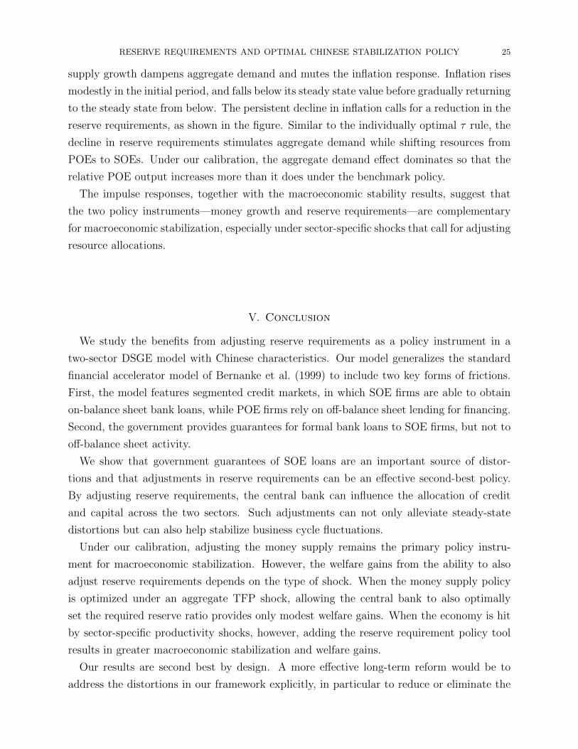
RESERVE REQUIREMENTS AND OPTIMAL CHINESE STABILIZATION POLICY 25
supply growth dampens aggregate demand and mutes the inflation response. Inflation rises
modestly in the initial period, and falls below its steady state value before gradually returning
to the steady state from below. The persistent decline in inflation calls for a reduction in the
reserve requirements, as shown in the figure. Similar to the individually optimal τ rule, the
decline in reserve requirements stimulates aggregate demand while shifting resources from
POEs to SOEs. Under our calibration, the aggregate demand effect dominates so that the
relative POE output increases more than it does under the benchmark policy.
The impulse responses, together with the macroeconomic stability results, suggest that
the two policy instruments—money growth and reserve requirements—are complementary
for macroeconomic stabilization, especially under sector-specific shocks that call for adjusting
resource allocations.
V. Conclusion
We study the benefits from adjusting reserve requirements as a policy instrument in a
two-sector DSGE model with Chinese characteristics. Our model generalizes the standard
financial accelerator model of Bernanke et al. (1999) to include two key forms of frictions.
First, the model features segmented credit markets, in which SOE firms are able to obtain
on-balance sheet bank loans, while POE firms rely on off-balance sheet lending for financing.
Second, the government provides guarantees for formal bank loans to SOE firms, but not to
off-balance sheet activity.
We show that government guarantees of SOE loans are an important source of distor-
tions and that adjustments in reserve requirements can be an effective second-best policy.
By adjusting reserve requirements, the central bank can influence the allocation of credit
and capital across the two sectors. Such adjustments can not only alleviate steady-state
distortions but can also help stabilize business cycle fluctuations.
Under our calibration, adjusting the money supply remains the primary policy instru-
ment for macroeconomic stabilization. However, the welfare gains from the ability to also
adjust reserve requirements depends on the type of shock. When the money supply policy
is optimized under an aggregate TFP shock, allowing the central bank to also optimally
set the required reserve ratio provides only modest welfare gains. When the economy is hit
by sector-specific productivity shocks, however, adding the reserve requirement policy tool
results in greater macroeconomic stabilization and welfare gains.
Our results are second best by design. A more effective long-term reform would be to
address the distortions in our framework explicitly, in particular to reduce or eliminate the

RESERVE REQUIREMENTS AND OPTIMAL CHINESE STABILIZATION POLICY 26
distortion from the government guarantees on SOE loans. More broadly, our analysis sug-
gests potential welfare gains from coordination between banking regulations and monetary
policy in China.

RESERVE REQUIREMENTS AND OPTIMAL CHINESE STABILIZATION POLICY 27
References
Basu, S. and J. G. Fernald (1997). Returns to scale in u.s. production: Estimates and
implications. Journal of Political Economy 105 (2), 249–283.
Bernanke, B., M. Gertler, and S. Gilchrist (1999). The financial accelerator in a quanti-
tative business cycle framework. In J. B. Taylor and M. Woodford (Eds.), Handbook of
Macroeconomics, pp. 1341–1393. Amsterdam, New York, and Oxford: Elsevier Science.
Brandt, L. (2015). Policy perspectives from the bottom up: What do firm-level data tell
us China needs to do? In R. Glick and M. M. Spiegel (Eds.), Policy Challenges in a
Diverging Global Economy: Proceedings from the 2015 Asia Economic Policy Conference,
San Francisco, CA. Federal Reserve Bank of San Francisco: Federal Reserve Bank of San
Francisco.
Brandt, L., C.-T. Hsieh, and X. Zhu (2008). Growth and structural transformation in China.
In L. Brandt and T. G. Rawski (Eds.), China’s Great Economic Transformation, pp. 683–
728. Cambridge University Press.
Brandt, L. and X. Zhu (2000). Redistribution in a decentralized economy. Journal of Political
Economy 108 (2), 422–439.
Chang, C., K. Chen, D. F. Waggoner, and T. Zha (2015). Trends and cycles in China’s
macroeconomy. In M. Eichenbaum and J. Parker (Eds.), NBER Macroeconomics Annual
2015, Volume 30, pp. 1–84. University of Chicago Press.
Chang, C., Z. Liu, and M. M. Spiegel (2015). Capital controls and optimal Chinese monetary
policy. Journal of Monetary Economics 74, 1–15.
Chang, C., Z. Liu, M. M. Spiegel, and J. Zhang (2017). Reserve requirements and optimal
Chinese stabilization policy. Federal Reserve Bank of San Francisco Working Paper 2016-
10.
Chen, K., P. Higgins, D. F. Waggoner, and T. Zha (2017, September). Impacts of monetary
stimulus on credit allocation and macroeconomy: Evidence from China. NBER Working
Paper No. 22650.
Chen, K., J. Ren, and T. Zha (2016, March). What we learn from China’s rising shadow
banking: Exploring the nexus of monetary tightening and banks’ role in entrusted lending.
Unpublished Manuscript, Emory University and the Federal Reserve Bank of Atlanta.
Chen, K., J. Ren, and T. Zha (2017, May). The nexus of monetary policy and shadow
banking in China. NBER Working Paper No. 23377.
Christiano, L. J., M. Eichenbaum, and C. L. Evans (2005). Nominal rigidities and the
dynamic effects of a shock to monetary policy. Journal of Political Economy 113 (1),
1–45.

RESERVE REQUIREMENTS AND OPTIMAL CHINESE STABILIZATION POLICY 28
Cong, L. W. and J. Ponticelli (2017, February). Credit allocation under economic stimulus:
Evidence from China. Unpublished Manuscript, University of Chicago Booth School of
Business.
Cun, W. and J. Li (2017, July). Sterilized intervention, bank credit, and Chinese monetary
policy. Unpublished Manuscript, USC Dornsife and Cantral University of Finance and
Economics.
Elliott, D., A. Kroeber, and Y. Qiao (2015). Shadow banking in China: A primer. The
Brooking Institution.
Federico, P., C. A. Vegh, and G. Vuletin (2014, October). Reserve requirement policy over
the business cycle. NBER Working Paper No. 20612.
Funke, M., P. Mihaylovski, and H. Zhu (2015, September). Monetary policy transmission in
China: A DSGE model with parallel shadow banking and interest rate control. Bank of
Finland BOFIT Discussion Papers.
Hachem, K. and Z. M. Song (2015). The rise of Chinas shadow banking system. Unpublished
manuscript, Chicago Booth.
Hsieh, C.-T. and P. J. Klenow (2009, November). Misallocation and manufacturing TFP in
China and India. The Quarterly Journal of Economics 124 (4), 1403–1448.
Hsieh, C.-T. and Z. M. Song (2015, March). Grasp the large, let go of the small: The trans-
formation of the state sector in China. In J. C. Eberly and J. H. Stock (Eds.), Brookings
Papers on Economic Activity, Volume Spring, pp. 295–366. The Brookings Institution.
Liu, Z., P. Wang, and T. Zha (2013, May). Land-price dynamics and macroeconomic fluc-
tuations. Econometrica 81 (3), 1147–1184.
Lu, Y., H. Guo, E. H. Kao, and H.-G. Fung (2015). Shadow banking and firm financing in
China. International Review of Economics and Finance 36, 40–53.
Montoro, C. and R. Moreno (2011, March). The use of reserve requirements as a policy
instrument in Latin America. BIS Quarterly Review , 53–65.
Rotemberg, J. J. (1982). Sticky prices in the United States. Journal of Political Econ-
omy 90 (6), 1187–1211.
Smets, F. and R. Wouters (2007). Shocks and frictions in US business cycles: A Bayesian
DSGE approach. American Economic Review 97 (3), 586–606.
Song, Z., K. Storesletten, and F. Zilibotti (2011). Growing like China. American Economic
Review 101 (1), 196–233.
Wang, H., H. Wang, L. Wang, and H. Zhou (2016, May). Shadow banking: China’s dual-
track interest rate liberalization. Unfinished Manuscript, Tsinghua University.
Zhu, X. (2012). Understanding China’s growth: Past, present, and future. Journal of
Economic Perspectives 26 (4), 103–124.

RESERVE REQUIREMENTS AND OPTIMAL CHINESE STABILIZATION POLICY 29
Table 1. Announcement Effects of RR policy on stock returns
Event window 1-day (H=0) 3-day (H=1) 5-day (H=2)
∆RRt−1 0.00206 0.00479 0.01057
(7.20) (9.21) (15.74)
SOEjt × ∆RRt−1 -0.0012 -0.00225 -0.00442
(-3.21) (-3.32) (-5.05)
SOEjt -0.00007 -0.00026 -0.00041
(-2.60) (-5.29) (-6.47)
Firm size -0.00034 -0.00099 -0.00155
(-27) (-43) (-53)
Book-to-market ratio 0.00009 0.00024 0.00047
(2.22) (3.29) (4.96)
Industry fixed effects Y Y Y
Year fixed effects Y Y Y
Sample size 4,119,971 4,079,847 4,0003,53
R2 0.00071 0.00182 0.00288
Note: For each coefficient, the upper row displays the estimated valued and the numbers
shown in parantheses are the t-statistics. The critical values of t-statistics are 1.64. 1.96,
and 2.58 for the 10%, 5%, and 1% significance levels, respectively.

RESERVE REQUIREMENTS AND OPTIMAL CHINESE STABILIZATION POLICY 30
Table 2. Announcement Effects of RR policy on stock returns: Before and
after fiscal stimulus
Pre-stimulus (2005-2008) Post-stimulus (2009-2015)
Event window 1-day (H=0) 3-day (H=1) 1-day (H=0) 3-day (H=1)
∆RRt−1 0.0010 0.0003 0.0029 0.0081
(2.00) (0.31) (8.08) (12.57)
SOEjt × ∆RRt−1 0.0001 0.0012 -0.0024 -0.0046
(0.11) (1.03) (-4.78) -5.03
SOEjt 0.00002 0.0005 -0.0002 -0.0005
(2.90) (4.09) (-4.85) (-8.86)
Firm size -0.0003 -0.0008 -0.0004 -0.0011
(-9) (-14) (-26) (-41)
Book-to-market ratio 0.0000 0.0001 0.0001 0.0004
(-0.25) (-0.56) (2.91) (4.50)
Industry fixed effects Y Y Y Y
Year fixed effects Y Y Y Y
Sample size 1,018,628 1,003,518 3,101,343 3,076,329
R2 0.0005 0.0011 0.0008 0.0022
Note: For each coefficient, the upper row displays the estimated valued and the numbers
shown in parantheses are the t-statistics. The critical values of t-statistics are 1.64. 1.96,
and 2.58 for the 10%, 5%, and 1% significance levels, respectively.

RESERVE REQUIREMENTS AND OPTIMAL CHINESE STABILIZATION POLICY 31
Table 3. Calibrated values.
Variable Description Value
A. Households
β Subjective discount factor 0.995
η Inverse Frisch elasticity of labor supply 2
Ψ Weight of disutility of working 18
δ Capital depreciation rate 0.035
Ωk Capital adjustment cost 1
B. Retailers
ε Elasticity of substitution between retail products 10
Ωp Price adjustment cost parameter 22
C. Firms and financial intermediaries
g Steady state growth rate 1.0125
k Shape parameter in Pareto distribution of idiosyncratic shocks 1.587
ωm Scale parameter in Pareto distribution of idiosyncratic shocks 0.37
As SOE TFP scale (normalized) 1
Ap POE TFP scale 1.42
α Capital income share 0.5
θ Share of household labor 0.94
ψ Share parameter for SOE output in intermediate good 0.45
σ Elasticity of substitution between SOE and POE products 3
ms SOE monitoring cost 0.15
mp POE monitoring cost 0.15
ξs SOE manager’s survival rate 0.97
ξp POE manager’s survival rate 0.69
D. Government policy
π Steady state inflation rate 1.005
τ Required reserve ratio 0.15
ψmp Money growth rule coefficient for inflation −0.65
ψmy Money growth rule coefficient for output 0.30G
GDPShare of government spending in GDP 0.14
ls Fraction of SOE debt guaranteed by the government 1
lp Fraction of SOE debt guaranteed by the government 0
E. Shock process
ρa Persistence of TFP shock 0.95
σa Standard deviation of TFP shock 0.01

RESERVE REQUIREMENTS AND OPTIMAL CHINESE STABILIZATION POLICY 32
Table 4. Volatilities and welfare under alternative policy rules
Variables (1) Benchmark (2) Optimal τ rule (3) Optimal money rule (4) Jointly optimal rule
Panel A: Aggregate TFP shock
Policy rule coefficients
ψmp −0.65 −0.65 −47.54 −63.40
ψmy 0.30 0.30 2.68 −12.50
ψτp 0.00 32.06 0.00 357.89
ψτy 0.00 −2.42 0.00 −19.26
Volatility and welfare
GDP 5.284% 5.231% 5.220% 5.205%
π 0.517% 0.076% 0.020% 0.064%
C 4.422% 4.373% 4.356% 4.363%
Ys 5.352% 5.369% 5.305% 5.515%
Yp 5.434% 5.523% 5.525% 5.430%
Welfare gains — 0.0280% 0.0275% 0.0281%
Panel B: POE-specific TFP shock
Policy rule coefficients
ψmp −0.65 −0.65 −45.42 −2.44
ψmy 0.30 0.30 4.42 −1.42
ψτp 0.00 35.44 0.00 28.18
ψτy 0.00 −4.40 0.00 −5.61
Volatility and welfare
GDP 3.828% 3.817% 3.809% 3.812%
π 0.180% 0.067% 0.046% 0.093%
C 3.284% 3.275% 3.273% 3.288%
Ys 2.848% 2.830% 2.817% 2.727%
Yp 6.549% 6.539% 6.529% 6.518%
Welfare gains — 0.0031% 0.0032% 0.0040%

RESERVE REQUIREMENTS AND OPTIMAL CHINESE STABILIZATION POLICY 33
0
5
10
15
20
25
2004 2005 2006 2007 2008 2009 2010 2011 2012 2013 2014 2015 Source:Bloomberg
China required reserve ratio Percent
Figure 1. China’s required reserve ratio (daily frequencies).

RESERVE REQUIREMENTS AND OPTIMAL CHINESE STABILIZATION POLICY 34
-0.0441
0
0.0210Heavy industry loan (log)
-6.3766
0
5.2763#10 -3 SOE investment share
-2.7171
0
2.1823#10 -3 Lending rate
4 8 12 16-0.0187
0
0.0109Required reserve ratio
Figure 2. Impulse responses of heavy industry loans, SOE investment share,
one-year benchmark lending interest rate, the required reserve ratio (RRR)
following a shock to RRR in an estimated BVAR model.

RESERVE REQUIREMENTS AND OPTIMAL CHINESE STABILIZATION POLICY 35
0 5 10 15 200.7
0.8
0.9
1
perc
ent d
evia
tions
Real GDP
0 5 10 15 20-0.6
-0.4
-0.2
0
0.2
perc
ent d
evia
tions
Inflation
0 5 10 15 20-15
-10
-5
0
5
perc
ent d
evia
tions
Money growth rate
0 5 10 15 20-100
-50
0
50
perc
ent d
evia
tions
Required reserve ratio
0 5 10 15 20-0.5
0
0.5
1
1.5
perc
ent d
evia
tions
SOE output
0 5 10 15 200.5
1
1.5
2
perc
ent d
evia
tions
POE output
0 5 10 15 20-30
-20
-10
0
10
perc
ent d
evia
tions
SOE bankruptcy ratio
Impulse responses to TFP shock
0 5 10 15 20-100
0
100
200
300
perc
ent d
evia
tions
POE bankruptcy ratio
BenchmarkOptimal money supply ruleOptimal ruleJointly optimal rules
Figure 3. Impulse responses to a positive TFP shock under alternative pol-
icy rules. Benchmark rule: black solid lines; optimal money growth rule: blue
dashed lines; optimal reserve requirement rule: red dashed lines; jointly opti-
mal rule: magenta dashed lines. The horizontal axes show the quarters after
the impact period of the shock. The units on the vertical axes are percent
deviations from the steady state levels.

RESERVE REQUIREMENTS AND OPTIMAL CHINESE STABILIZATION POLICY 36
0 5 10 15 200.55
0.6
0.65
0.7
perc
ent d
evia
tions
Real GDP
0 5 10 15 20-0.1
0
0.1
0.2
perc
ent d
evia
tions
Inflation
0 5 10 15 20-2
-1
0
1
2
perc
ent d
evia
tions
Money growth rate
0 5 10 15 20-20
-10
0
10
perc
ent d
evia
tions
Required reserve ratio
0 5 10 15 20-1.5
-1
-0.5
0
perc
ent d
evia
tions
SOE output
0 5 10 15 200.5
1
1.5
2
perc
ent d
evia
tions
POE output
0 5 10 15 20-5
0
5
10
perc
ent d
evia
tions
SOE bankruptcy ratio
Impulse responses to POE TFP shock
0 5 10 15 20-100
0
100
200
perc
ent d
evia
tions
POE bankruptcy ratio
BenchmarkOptimal money supply ruleOptimal ruleJointly optimal rules
Figure 4. Impulse responses to a positive POE TFP shock under alternative
policy rules. See the caption under Figure 3 for an explanation of lines and
the units of the axes.