1

““RReesseeaarrcchhiinngg tthhee TTrraaddee PPrroodduuccttiivviittyy LLiinnkk::

EEvviiddeennccee ffrroomm UUrruugguuaayy””

Preliminary Draft

AAddrriiaannaa PPeelluuffffoo ((**))

Acknowledgements I would like to thank Dr. Calfat for his help, and to the Professors of the Department of Economics, School of Social Sciences, University of Uruguay, especially to Prof. M. Vaillant, G. Romaniello, A. Cassoni, I. Terra and R. Patron. I am indebted also to MSc. Daniela Cristina for her help and support. Remaining errors are of my own.

(*) University of Antwerp, Alfa Programme; Universidad de la República, Uruguay.

2

Abstract

Development economists argue that trade protection reduces industrial sector efficiency, mainly through the distortion in relative prices, increased market power, x-inefficiency and inefficient scales of production. Nevertheless there is no convincing evidence on the link between trade reforms and improvement in economic performance.

This work examines the case of Uruguay, an economy that introduced major trade reforms initially in the mid-1970s with a continuous reduction in trade barriers in the 1980s. In 1991, this process was deepened with the signature of the Asuncion Treaty aimed to the creation of the Southern Common Market.

Thus the objective of this work is to analyse the impact of trade liberalisation –namely the increase in liberalisation as a result of the creation of the MERCOSUR -on economic performance for the Uruguayan case, in the period 1990-1994. To do so we estimate returns to scale for 37 branches at a 4-digit ISIC code level, as well as efficiency and dispersion, using a Cobb-Douglas production function. We kept the results only for 19 branches with unitary returns to scale and then we calculate the Spearman’s rank correlation coefficient between changes in scale, efficiency dispersion and changes in average rate of protection, nominal rate of protection and import penetration. The results did not show any significant association of the trade indicators with returns to scale.

Then we estimate changes in labour productivity and price cost margins for 68 branches at a 4-digit ISIC code level. As explanatory variables we calculate a set of alternative indicators of trade liberalisation, as well as industrial structure and technology variables. We use the indicators of trade liberalisation, structure and technology variables to explain changes in economic performance in a cross- sectional regression model for the years 1990 and 1994.

As many others other empirical works, our results are far from conclusive. While there is some weak evidence of a positive effect of trade liberalisation the results point out the importance of technology and market structures variables. Thus we can not expect that trade liberalisation was the only instrument to improve performance of the industrial sector in developing countries, and as the results shows there is still a role for policies aimed to promote competition and technological change.

3

Table of Contents

Introduction

I. Liberalization and Performance

II. Trade Policy in Uruguay

III. The Manufacturing Industry in Uruguay

IV. The Model

IV.1 Returns to scale IV.2 Changes in labour productivity and price-cost margins

V. Results

Conclusions

References

Appendices

List of Tables

Table 1: Tariff schedule, 1992. Table 2: Evolution of the Uruguayan Economy, 1990-1994. Table 3: Evolution of the Manufacturing Industry, 1990-1994. Table 4: Estimates of Returns to Scale, Efficiency and Dispersion in levels for 1990 and 1994and ratios at a 4-ISIC code level. Table 5: Spearman’s rank correlation coefficients between ratios of efficiency, dispersion and returns to scale ratios, and trade liberalization variables in ratios. Table 6: Regression equations for changes in labour productivity corrected for heteroscedasticity. Table 7: Regression Equations for Changes in Price-Cost Margins (after correcting for heteroscedasticity). Table 8: Regression Equations for changes in Price-Cost Margins for more concentrated corrected for heteroscedasticity.

Appendices

Appendix 1: Changes in nominal rate of protection and weighted average rate of protection, at a 4-digit ISIC code level, 1990-1994. Appendix 2: Changes in import penetration by industry, 4-digit ISIC code level, 1990-1994.

4

Introduction

Development economists argue that trade protection reduces industrial sector efficiency, mainly through the distortion in relative prices, increased market power, x-inefficiency and inefficient scales of production. Moreover, trade policy reform has been a central feature of the economic adjustment programs introduced in many developing countries in recent years.

Nevertheless, there is no convincing evidence on the link between trade reforms and improvement in economic performance. Empirical evidence is relatively scarce and often ambiguous (Pack, 1988, Havrylyshyn, 1990; Tybout, 1992). Pack (1988) notes that: “to date there is no clear confirmation of the hypothesis that countries with an external orientation benefit from greater growth in technical efficiency in the component sector of manufacturing”. The results may depend on the initial level of efficiency of firms, as well as other macro and micro policies of the country of concern, while other strand of the literature points out the importance of the strategies carried out by the firms to develop the so called ‘competitive advantages’.

This work examines the case of Uruguay, an economy that introduced major trade reforms initially in the mid-1970s with a continuous reduction in trade barriers in the 1980s. In 1991, this process was deepened with the signature of the Asuncion Treaty aimed to the creation of the Southern Common Market.

Thus, the objective of this work is to analyse the impact of trade liberalisation on on returns to scale, labour productivity and price-cost margins. We work at a 4-digit ISIC code level for the years 1990 and 1994. We use two distinct approaches. For changes in returns to scale we analyse its association with changes in a set of trade liberalisation variables. While for changes in labour productivity and price-cost margins we estimate cross sectional regression models taking as explanatory variables a set of alternative indicators of trade liberalisation as well as industrial and technology variables.

This work structures as follow: first we briefly mention the main links between trade liberalisation and performance. Then we comment the main features of trade policy, and give a quick description of the manufacturing industry in Uruguay. Then, we present the methodology used and, finally our main results and conclusions.

I. Theoretical Issues

There are three main arguments to link trade liberalisation and economic performance1. One is the well known ‘resource reallocation effect’. In the presence of perfectly competitive markets, trade liberalisation will change the set of relative prices in line with world prices, and the producers will respond to this new set of prices reallocating resources according to the comparative advantage of the countries. This is the standard gain associated with a move towards free trade.

1 Pack (1988) and Havrylyshyn (1990) surveyed the mechanisms by which trade liberalisation may improve performance.

5

In the presence of imperfectly competitive markets, trade liberalisation may bring additional

gains. The potential or actual competition of imports will stimulate producers to lower their x-inefficiency. Even more, when competitive discipline is absent producers will enjoy monopoly power, which in turn may allow inefficient firms to survive. Thus, liberalisation is expected to reduced deadweight losses due to market power (pro-competitive effect), increase firms size and scale efficiency.

Finally, liberalisation is expected to induce a higher long run rate of growth through greater technical change and access to economies of scale in an open environment. These dynamic effects are associated with a higher growth path and so with cumulative improvements over time.

The speed at which these effects would operate is variable. Generally, it is assumed that the initial shock effect and the reallocation of resources effect will operate in a four-year period while the dynamic effects will take a longer period to be felt.

Nevertheless, as pointed out by Tybout (1991), Weiss (1991), and Rodrik (1988ª) these effects are not inevitable. Whether trade liberalisation improves efficiency will depend on the distribution of output adjustment across plants with differing unit costs (Rodrik, 1988ª). This will depend on factor intensities, the pattern of demand shifts, the nature of competition and the extent into which entry and exit are possible. Ease of entry and exit would moderate the effect of trade liberalisation on size and productivity (Roberts and Tybout, 1991). Furthermore, when technology and innovation are endogenous further ambiguities result (Rodrik, 1988b).

Thus, even though some simulation models support that in LDC’s liberalisation of imperfectly competitive industries results in larger plants and higher efficiency (Condon and de Melo, 1986; Devarajan and Rodrik, 1989ª, 1989b; de Melo and Roland-Holst, 1991 cited by Roberts and Tybout, 1991), empirical support is scarce. In this regard Bhagwatti (1988) concludes that: “Although the arguments for the success of [outward-oriented development strategies] based on economies of scale and x-efficiency are plausible, empirical support for them is not available”.

There are various possible levels of analysis: at the economy wide level, at the sectoral and

industry level and at the firm level.

At the economy wide level some studies for Latin America show mixed results. Most studies suggest that the region average total factor productivity growth was negative or low for the decade of the 1990s, when most countries en the region reduced their trade barrier (IDB, 2001; Baier, Dwyer Jr., Tamura, 2002; Loyaza, Fajnzylber and Calderon, 2002). These studies show significant heterogeneity in the country’s TFP performance in relation to the decade of the 1980s. This could be telling us that gains from increased openness were not strong enough to offset the negative influences on productivity such as macroeconomic volatility.

At the sectoral level studies for the manufacturing sector for Argentina, Brazil and Mexico, show a considerable increase in labour productivity, though it should be note that this is a partial indicator of productivity (Lopez-Cordova, 2003).

Studies based on firm level data report increase in total factor productivity during the trade liberalization period for Mexico, Brazil, Chile, Colombia: report positive rates of growth in manufacturing during the trade liberalization period (Lopez-Cordova and Mesquita, 2003; Tybout and Westbrook, 1995; Muendler, 2002; Pavcnik, 2000; Fernandes, 2001). They also find evidence

6

of the trade productivity links mainly through import discipline effects. Nevertheless, the number of countries studied is still limited and some methodological hurdles have yet to be overcome (Tybout, 2001; Katayama, Lu and Tybout, 2003).

Thus, this work is an attempt to gather some preliminary empirical evidence for the Uruguayan case.

II. Trade Policy in Uruguay

As most countries in the region, Uruguay have pursued an import substitution policy from the earlier 1950s to mid-70s.Since 1974 Uruguay has experienced a continuous decrease in the tariff barriers that protected domestic production. Also different non- tariff barriers as quotas, licenses and prohibitions, were eliminated2.

At the beginning of the 80’s imports were regulated mainly through tariffs (taxes on imports) and reference prices. The process of tariff reduction can be divided into four distinct stages: 1. Between 1974 and 1979 non- tariff barriers (as quotas, licenses, prohibitions) were eliminated,

and reductions in tariffs were approved. In 1974 the higher tariff was 300 % and decreased to 90 % in 1979.

2. In 1980 a second stage can be identified. It was characterised by a gradual and progressive

reduction in the number and the level of tariffs with the goal to end in a unique tariff of 35 % in a five-year period. Nevertheless, it could not been achieved due to the external crisis that lead to adjustments in the exchange rate policy in 1982.

3. In 1983 a new regimen started, and instead of a single tax as was intended in the preceding

program, 5 tariffs levels were established according to the nature and utilisation of the imported goods, as well as it effective rate of protection. Imports of raw materials whose production were not economically feasible in our country were charge with a minimum tariff of 10 %. On the other hand tariffs of 20 %, 35 %, and 45 %, were charged on intermediate goods and final goods of reduced value added. Finally, those final goods with higher value added were charged with a maximum tariff of 55 %.

4. The new administration that took place in 1990 set an increase of 5 % for all tariffs levels except

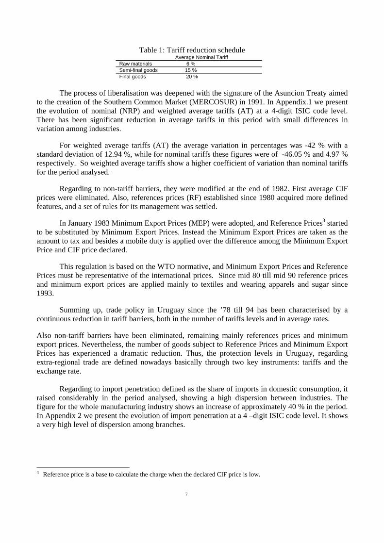
those of 35 and 45 %, in order to reduce the fiscal deficit. At the same time were announced reductions in tariffs that would be applied from September 1991, with only 3 tariffs levels of 10, 20, and 30 %, continuing with the policy of decreasing tariffs to a maximum of 20 %. Since January 1992 the following schedule took place:

2 Trade policy in Uruguay was surveyed by M. Vaillant (1998).

7

Table 1: Tariff reduction schedule Average Nominal Tariff Raw materials 6 % Semi-final goods 15 % Final goods 20 %

The process of liberalisation was deepened with the signature of the Asuncion Treaty aimed

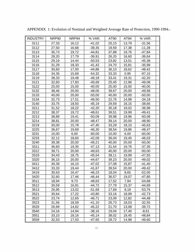
to the creation of the Southern Common Market (MERCOSUR) in 1991. In Appendix.1 we present the evolution of nominal (NRP) and weighted average tariffs (AT) at a 4-digit ISIC code level. There has been significant reduction in average tariffs in this period with small differences in variation among industries.

For weighted average tariffs (AT) the average variation in percentages was -42 % with a standard deviation of 12.94 %, while for nominal tariffs these figures were of -46.05 % and 4.97 % respectively. So weighted average tariffs show a higher coefficient of variation than nominal tariffs for the period analysed.

Regarding to non-tariff barriers, they were modified at the end of 1982. First average CIF prices were eliminated. Also, references prices (RF) established since 1980 acquired more defined features, and a set of rules for its management was settled.

In January 1983 Minimum Export Prices (MEP) were adopted, and Reference Prices3 started to be substituted by Minimum Export Prices. Instead the Minimum Export Prices are taken as the amount to tax and besides a mobile duty is applied over the difference among the Minimum Export Price and CIF price declared.

This regulation is based on the WTO normative, and Minimum Export Prices and Reference Prices must be representative of the international prices. Since mid 80 till mid 90 reference prices and minimum export prices are applied mainly to textiles and wearing apparels and sugar since 1993.

Summing up, trade policy in Uruguay since the ’78 till 94 has been characterised by a continuous reduction in tariff barriers, both in the number of tariffs levels and in average rates.

Also non-tariff barriers have been eliminated, remaining mainly references prices and minimum export prices. Nevertheless, the number of goods subject to Reference Prices and Minimum Export Prices has experienced a dramatic reduction. Thus, the protection levels in Uruguay, regarding extra-regional trade are defined nowadays basically through two key instruments: tariffs and the exchange rate.

Regarding to import penetration defined as the share of imports in domestic consumption, it raised considerably in the period analysed, showing a high dispersion between industries. The figure for the whole manufacturing industry shows an increase of approximately 40 % in the period. In Appendix 2 we present the evolution of import penetration at a 4 –digit ISIC code level. It shows a very high level of dispersion among branches.

3 Reference price is a base to calculate the charge when the declared CIF price is low.

8

III. The Manufacturing Industry in Uruguay

As most countries in Latin America the manufacturing industries in Uruguay were developed in the context of import substituting policies, which implied a high level of protection to domestic production.

Uruguayan firms are relatively small –as a result of the small size of the country – and domestic markets are characterised by a relatively high concentration and oligopolistic market structures.

In the ’70 a process of liberalisation started, as well as policies aimed to structural

adjustment of the economy. In 1991, Uruguay joined to a Regional Integration Agreement, with the signature of the Asuncion Treaty aimed to the creation of the Southern Custom Union (MERCOSUR), deepening the liberalisation process.

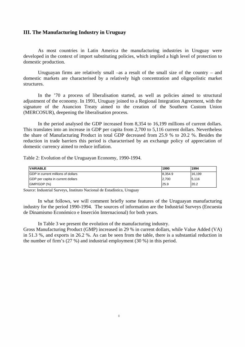
In the period analysed the GDP increased from 8,354 to 16,199 millions of current dollars. This translates into an increase in GDP per capita from 2,700 to 5,116 current dollars. Nevertheless the share of Manufacturing Product in total GDP decreased from 25.9 % to 20.2 %. Besides the reduction in trade barriers this period is characterised by an exchange policy of appreciation of domestic currency aimed to reduce inflation. Table 2: Evolution of the Uruguayan Economy, 1990-1994.

VARIABLE 1990 1994 GDP in current millions of dollars 8,354.9 16,199 GDP per capita in current dollars 2,700 5,116 GMP/GDP (%) 25.9 20.2

Source: Industrial Surveys, Instituto Nacional de Estadística, Uruguay

In what follows, we will comment briefly some features of the Uruguayan manufacturing industry for the period 1990-1994. The sources of information are the Industrial Surveys (Encuesta de Dinamismo Económico e Inserción Internacional) for both years.

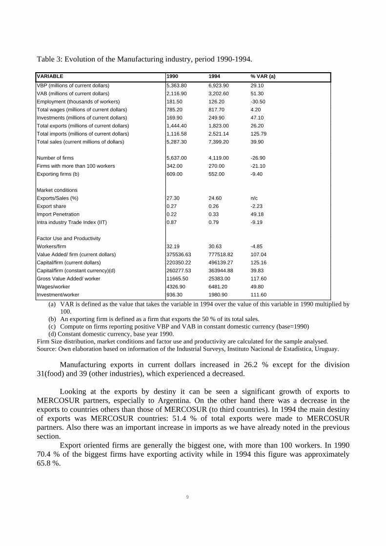
In Table 3 we present the evolution of the manufacturing industry. Gross Manufacturing Product (GMP) increased in 29 % in current dollars, while Value Added (VA) in 51.3 %, and exports in 26.2 %. As can be seen from the table, there is a substantial reduction in the number of firm’s (27 %) and industrial employment (30 %) in this period.

9

Table 3: Evolution of the Manufacturing industry, period 1990-1994. VARIABLE 1990 1994 % VAR (a)

VBP (millions of current dollars) 5,363.80 6,923.90 29.10 VAB (millions of current dollars) 2,116.90 3,202.60 51.30 Employment (thousands of workers) 181.50 126.20 -30.50 Total wages (millions of current dollars) 785.20 817.70 4.20 Investments (millions of current dollars) 169.90 249.90 47.10 Total exports (millions of current dollars) 1,444.40 1,823.00 26.20 Total imports (millions of current dollars) 1,116.58 2,521.14 125.79 Total sales (current millions of dollars) 5,287.30 7,399.20 39.90 Number of firms 5,637.00 4,119.00 -26.90 Firms with more than 100 workers 342.00 270.00 -21.10 Exporting firms (b) 609.00 552.00 -9.40 Market conditions Exports/Sales (%) 27.30 24.60 n/c Export share 0.27 0.26 -2.23 Import Penetration 0.22 0.33 49.18 Intra industry Trade Index (IIT) 0.87 0.79 -9.19 Factor Use and Productivity Workers/firm 32.19 30.63 -4.85 Value Added/ firm (current dollars) 375536.63 777518.82 107.04 Capital/firm (current dollars) 220350.22 496139.27 125.16 Capital/firm (constant currency)(d) 260277.53 363944.88 39.83 Gross Value Added/ worker 11665.50 25383.00 117.60 Wages/worker 4326.90 6481.20 49.80 Investment/worker 936.30 1980.90 111.60

(a) VAR is defined as the value that takes the variable in 1994 over the value of this variable in 1990 multiplied by 100.

(b) An exporting firm is defined as a firm that exports the 50 % of its total sales. (c) Compute on firms reporting positive VBP and VAB in constant domestic currency (base=1990) (d) Constant domestic currency, base year 1990.

Firm Size distribution, market conditions and factor use and productivity are calculated for the sample analysed. Source: Own elaboration based on information of the Industrial Surveys, Instituto Nacional de Estadística, Uruguay.

Manufacturing exports in current dollars increased in 26.2 % except for the division 31(food) and 39 (other industries), which experienced a decreased.

Looking at the exports by destiny it can be seen a significant growth of exports to MERCOSUR partners, especially to Argentina. On the other hand there was a decrease in the exports to countries others than those of MERCOSUR (to third countries). In 1994 the main destiny of exports was MERCOSUR countries: 51.4 % of total exports were made to MERCOSUR partners. Also there was an important increase in imports as we have already noted in the previous section.

Export oriented firms are generally the biggest one, with more than 100 workers. In 1990 70.4 % of the biggest firms have exporting activity while in 1994 this figure was approximately 65.8 %.

10

Total investments increased in 47.1 % in the period, while total sales in current dollars, and investments per worker growth in 101.3 % and 111.6 % respectively. In both years manufacturing investment was concentrated in 3 divisions: food (31), textiles (32) and chemicals (35), which accumulated approximately 75 % of total investments.

Firms with more than 100 workers and exporting activity made almost half of total

investment in both years. Regarding to foreign participation, in 1990, as well in as in 1994, firms with participation of foreign capital carried out the 27 % of total investments. The increase in investment along with the reduction (of 26.9 %) in the number of firms in this period resulted in an increase of 101.3 % of the average investment by firm.

At its time, the growth in value added, and the decrease in employment resulted in an increase in labour productivity (117.6 % in 1994 in relation to the year 1990). Though average wages by worker increased this increase was lower that the increase in labour productivity allowing an increase in price cost margins in the period analysed.

Regarding to size distribution measured in terms of number of workers we observe a decrease of 21 % in those firms with more than 100 workers.

Looking at factor use and productivity at the firm level we can observe a decrease in workers by firms (4.85 %), a substantial increase in value added per firm (107 %) and capital per firm (124.16 %), as well as in value added per worker (117.60 %).

As we already noted the manufacturing industry in Uruguay is characterised by an oligopolistic structure. We calculated the Herfindhal index, both in terms of gross output and in sales in the domestic market, and the C4 index. So we have 3 alternative indicators of markets structure that we denominate:

H=Σ(sij)2, where sij is the share of gross output of firm i belonging to industry j in total gross output of the industry. HC=Σ(DS/TDS+ IMP)2; where DS stands for domestic sales of firm i in industry j, TDS stands for total domestic sales in the industry, and IMP imports in the industry. C4= ΣDS4/(TDS+IMP), this is the sum of domestic sales of the four biggest firms in the industry over total domestic sales plus imports.

We found that for 1990, 25 out of 64 industries have a C4 index greater than 0.45 (40.62 % of the industries considered), while in 1994 this number decreased to 19 out of 64 (29.69 %). The average value of the C4 index in 1990 was 0.4589 while in 1994 was 0.37, with an average reduction of 7 %, though the variation between branches is quite high.

Finally, since we will work with average values of firms at the industry level, we should mention that various national studies point out the high heterogeneity among firms belonging to the same branch, though the degree to international exposure is the same (Departamento de Economía, 1994; Garcia and Tansini, 1996). Thus, we have to be cautious in interpreting the results. This high heterogeneity also may be a source of efficiency gains when manufacturing sector is exposed to increased competition (Tybout, 2001; Melitz, 2002; Lopez-Cordoba, 2003).

IV. Methodology

Our objective is to test whether trade liberalisation has had a positive effect on economic

performance in the Uruguayan manufacturing sector. We are particularly interested in analysing the impact on economies of scale, labour productivity and price-cost margins. We will use two distinct approaches: 1) for returns to scale we will estimate the Spearman’s rank correlation matrix between changes in returns to scale and changes in trade variables, 2) for changes in labour productivity and price cost margins we will estimate cross-sectional regression models. IV.1 Returns to scale

To analyse the impact of trade liberalisation on returns to scale we estimate a Cobb Douglas production function. We obtained estimates of efficiency, returns to scale and dispersion for both years, for 37 manufacturing branches at a 4-digit ISIC code level. Working with a lower level of aggregation (4-digit level) has the advantage of greater technological homogeneity among firms belonging to the same branch. Nevertheless, it has also has the shortcoming that we are left with fewer observations for each branch, which many times make no possible to estimate the production function4. Therefore we lost the estimates for those branches that are highly concentrated.

The function estimated was the following: ijIJjijjojij uEMPKVA +++= 21 βββ Where is gross value added for the iijVA th firm in the jth branch. is calculated as total wages for each firm in the branch divided by labour cost for the whole industry in the year analysed, while labour cost stands for the average wage at the branch level. Finally, is the capital stock. We take 1994 values to constant prices taking 1990 as the base year.

EMPij

Kij

All variables are in natural logarithms, and we estimated this function by OLS5.

While β 0 j gives estimates of efficiency (EF), β1 j +β 2 j gives returns to scale (RTS), while the variance of the residual term will give as an indicator of the dispersion of firms (DISPER).

Once we have the estimates, we construct industry specific indices of the changes in return to scale, average efficiency level (intercept of the production function) and dispersion in efficiency levels for the period analysed, as the following ratios: CRTS= RTS94/RTS90= (β1j + β2j)94/(β1j + β2j)90 CEF= EF94/EF90 = (β0j)94/(β0j)90 CDISP=DISPER94/DISPER90= (σ2

1j)94/(σ21j)90

4 We estimate the production function at a 4-digit level only for those branches with 7 or more observations.

11

5 We also estimate the production function through instrumental variables and Full Information Maximum Likelihood (FIML), in order to correct for mis-measurements in capital stock. Nevertheless, these estimates throw implausible low coefficients and a lower fit than the estimation using OLS, so they were disregarded. Possibly, the lower performance might have been due to the instrument used (total electrical energy consumed).

12

Working with ratios allow to ignore other macroeconomic shocks or data mis-measurement that affects all industries equally, as well as industry specific effects that do not vary over time.

Finally, we calculate the matrix of correlation (Spearman’s rank correlation coefficient) between indicators of trade liberalisation, returns to scale, efficiency, and dispersion (DISP).

Following Tybout et al. (1991) the hypothesis was that trade liberalisation would translate in an increase in efficiency (CEF), a reduction in the ratio of returns to scale (CRTS), and the dispersion ratio (CDISP). IV.2 Changes in labour productivity and price-cost margins

We define as indicators of economic performance labour productivity and price cost margins. We consider a set of explanatory variables that reflect industrial structure, technology and changes in trade policy. Then we apply OLS cross-sectional regression techniques to analyse the determinants of changes in performance.

The hypothesis that trade liberalisation has had a positive effect on economic performance will be demonstrated, if changes in the variables that reflect trade policy are significantly correlated with changes in performance indicators with the expected sign.

The regression model can be formally expressed as:

PI= f (TECH, STRUCT, TL)

Where: PI is a measure of change in a performance indicator; TECH stands for technology variables; STRUCT stands for variables reflecting industrial structure; TL is an indicator of change in trade policy.

All the indicators are calculated over the 1990-1994 period, as natural logarithm of the variable for 1994 minus the value that takes the variable in 1990. Proxies for industrial structure and technology were calculated for each single year and as rates of changes.

For each of the three sets of explanatory variables various alternatives specifications were

tested. In order to avoid collinearity problems those variables that are substitutes or are highly correlated are not used together in the same equation.

The data sources are the Industrial Surveys (Encuesta de Dinamismo Económico e Inserción Internacional) for the years 1990 and 1994. Also data on imports were provided by the Central Bank of Uruguay (Banco Central del Uruguay), and data on tariffs were provided by ALADI. IV.2.1 Dependent Variables: Performance Indicators

Empirical studies that have analysed the relationship between liberalisation and performance have used as indicators of performance measures of single or total factor productivity (TFP) growth, changes in price-cost margins (PCM) and export growth (Roberts and Tybout, 1996).

13

Productivity measures are to capture efficiency in input use, price-cost margins to reflect the extent to which domestic producers and price monopolistically.

In this work we will use as performance indicators labour productivity (LP) and price cost margins (PCM). Also an efficiency measure estimated through a Cobb Douglas production function for firms belonging to the same 4-digit level ISIC code6.Total Factor Productivity was disregarded7 in this first exploratory work since for the short run (as the period analysed) capital stock may be considered to be fixed. Also if there are not major changes in technology, labour productivity and Total Factor Productivity should be positively correlated.

Thus our estimates of changes in performance are:

i) Labour productivity (LP): is defined as the value added per worker at constant prices8. It was calculated as the average value for firms belonging to the same industry. An improvement in economic performance is given by an increase in labour productivity. ii) Price Cost Margin (PCM): is defined as value added minus wages over gross output (VBP) at current prices. Price-cost margins theoretically should compare price and marginal cost to assess the extent of non-competitive pricing. Here, as in other applied studies, a much cruder indicator is used with price-cost margins being measured by the ratio of economic surplus to gross output at current prices.

Collins and Preston (1968) introduced the concept of price-cost margins. This is defined as the difference between the price and the marginal costs divided by the price. Nevertheless, due to the difficulty to measure marginal cost in empirical studies average costs are used to approximate marginal costs. In so doing, we are implicitly assuming constant returns to scale. We should note that this indicator has been questioned because it does not consider capital costs. Furthermore, the level of price-cost margins will vary with the degree of capital-intensity in production, since the higher the capital-output ratio the higher must be price-cost margins for a given rate of return on capital. In terms of the impact of trade liberalisation it is change in price-cost margins that is of interest, with a fall in mark-ups (for a given capital-output ratio) interpreted as an improvement in performance due to more competitive pricing. Thus, the expectation is that with the actual or potential threat of import competition trade liberalisation will exert price discipline on domestic producers and thus it should have a negative effect on price-cost margins. IV.2.2 Explanatory variables

The regression model attempts to explain changes in performance indicators at the 4-digit ISIC level by three sets of explanatory variables related to i. Changes in trade policy towards an industry. ii. Technology and changes in technology used in an industry. iii. Industry structure and its changes at the industry level.

6 Also estimates of efficiency for a trans-logarithmic production function were tried as explanatory variables but the fit was so low that they were disregarded. 7 The estimation of TFP will be addressed in future works using panel data and a longer time interval. 8To carry out the deflation we used price indexes at a 3-digit level for VAB, VBP and capital.

14

i. Trade Liberalisation Variables For this study we use 3 types of indicators: a) Estimates of nominal (NRP) and average nominal tariffs (AT). b) Estimates of share of imports in total internal demand –import penetration- (IP). These are ex-post indicators of actual market penetration by imports9. c) A dummy that takes value of one when the branch is subject to Reference Prices or Minimum Export Prices. Since there are no estimates of coverage ratios of reference and minimum export prices for Uruguay, but as they are concentrated in textile and wearing apparels we use a dummy variable to capture its effect.

Of the alternative measures, trade liberalisation will be reflected in a fall trade variables except for import share in demand.

If the hypothesis on the link between improved performance and liberalisation is supported there will be a significant negative relation between changes in labour productivity and all liberalisation indicators except for import penetration, where the relation will be positive. For changes in price-cost margins the signs are reversed, since improved performance would imply a reduction in mark-ups. ii. Technology variables

The technology variables reflect the technology used by the firms belonging to the same industry. They were calculated both in terms of absolute value (level) for both years as well as in rates of changes. The variables used are proxies to capital intensity, an index of technology, and alternative indexes of scale. a) Capital intensity: capital-output ratio (KO) and capital-labour ratio (KL).

Capital-output ratio is defined as the value of capital assets in relation to gross output in an industry in 1990 and 1994. Capital-labour ratio is defined as the value of capital assets to number of employees. They give alternative measures of capital intensity. In so far as capital intensity is related to technical progress one would expect it to have a positive relation with growth in labour productivity and efficiency. However, the net effect of capital intensity on performance is ambiguous since it can also be a barrier to entry and thus hold back competitive pressure in an industry. When we take capital intensity in rate of changes, in order to interpret the results, we assume that the changes in this variable are mainly due to changes in output. b) Index of technology (IT)

The index of technology (IT) attempts to capture the technological diversity within a particular industry. This index is defined as the average productivity (average value added per worker) in an industry divided by the highest labour productivity in that particular industry). The higher is the index of technology the smaller will be the range of technology employed in the 9 Generally import penetration will follow trade liberalisation with a time lag, and it is influenced by the exchange rate policy.

15

industry. One would expect productivity growth to be negatively related to the index of technology since with low values of this variable there is greater scope for catching up as establishments who operate within the technology frontier improve their practices and move toward the frontier. c) Indexes of Scale (IS1)

This index of scale (different to the previous one obtained from the Cobb-Douglas production function) compares scale of production in an average firm with production in the industry divided by production in the largest size category of establishment in the industry. The indicator of scale (IS1) is calculated for both years, and it helps to capture diversity within a particular industry. The higher is IS1 the lower will be the range of production scales used in the industry.

One would expect changes in productivity to be negatively related to the index of scale, since the greater the range of scale of production the more scope for smaller enterprises to capture economies of scale by expansion. However, there is again an ambiguity, as a larger scale of production may also be a barrier to new entrants. A low index of scale (IS) may indicate that a potential new entrant may need to achieve scale of production well above average before it reaches a minimum efficient scale. If a low index of scale reflects a barrier to entry, then it could be positively rather than negatively associated with changes in performance.

iii. Market Structure Variables

The main structure variables used were output growth, concentration, foreign firm share and advertising intensity at the industry level. a. Output growth (OG): is defined as increase in gross output at constant prices. It was calculated as the average value for firms belonging to the same industry. Following the Verdoorn’s relation [Kaldor, 1967], one would expect it to be positively and closely correlated with changes in labour productivity, reflecting the importance of dynamic increasing returns. b. Concentration ratio (HC): is approximate through the Herfindhal index, which is defined as the sum of the squared market share of the firms belonging to the same 4-digit industry. Market share for firm i in industry j is defined as gross output value plus imports minus exports in relation to total sales in the industry. It is a more appropriate measure than the C4 index since it takes into account the number of firms in the industry.

As a measure of monopoly power, it is not clear a priori whether one would expect concentration to be positively or negative correlated with labour productivity. However, the ability to increase price mark-ups should be greater in more concentrated industries, so one would expect concentration and its changes to be positively correlated with a rise in price-cost margins, while a decrease should translate in lower mark ups. Moreover, it is expected that the higher the initial concentration of the industry the greater the reduction in mark-ups due to increased trade openness. c. Foreign firm share (FDI): is defined as total gross output of foreign firms in an industry over total gross output in that particular industry, calculated for both years. We defined a firm as foreign if more than 10 % of total capital is own by foreigners. In so far as foreign firms are technically and managerially more dynamic than others firms, one would expect a positive correlation between foreign presence and labour productivity. Foreign firms can be considered as particular agents,

16

whose features are different from domestic firms. With foreign direct investment not only capital is transferred, but also technology and know how. This makes that they may be considered as a mean of technological transfer for domestic firms. Thus, changes in foreign presence should be positively correlated with productivity gains. d. Advertising intensity (ADV): is defined as the share of advertising expenditure in total production value at the industry level for both years. It is a conventional measure of product differentiation. In the extent that advertising and brand loyalty create a further barrier to entry, advertising intensity can be expected to have a negative correlation with labour productivity and a positive correlation with changes in price-cost margins. We assume that the higher the initial advertising level the higher mark ups, and hence the more difficult to increase prices further.

17

V. Results

V.1 Changes in Returns to Scale

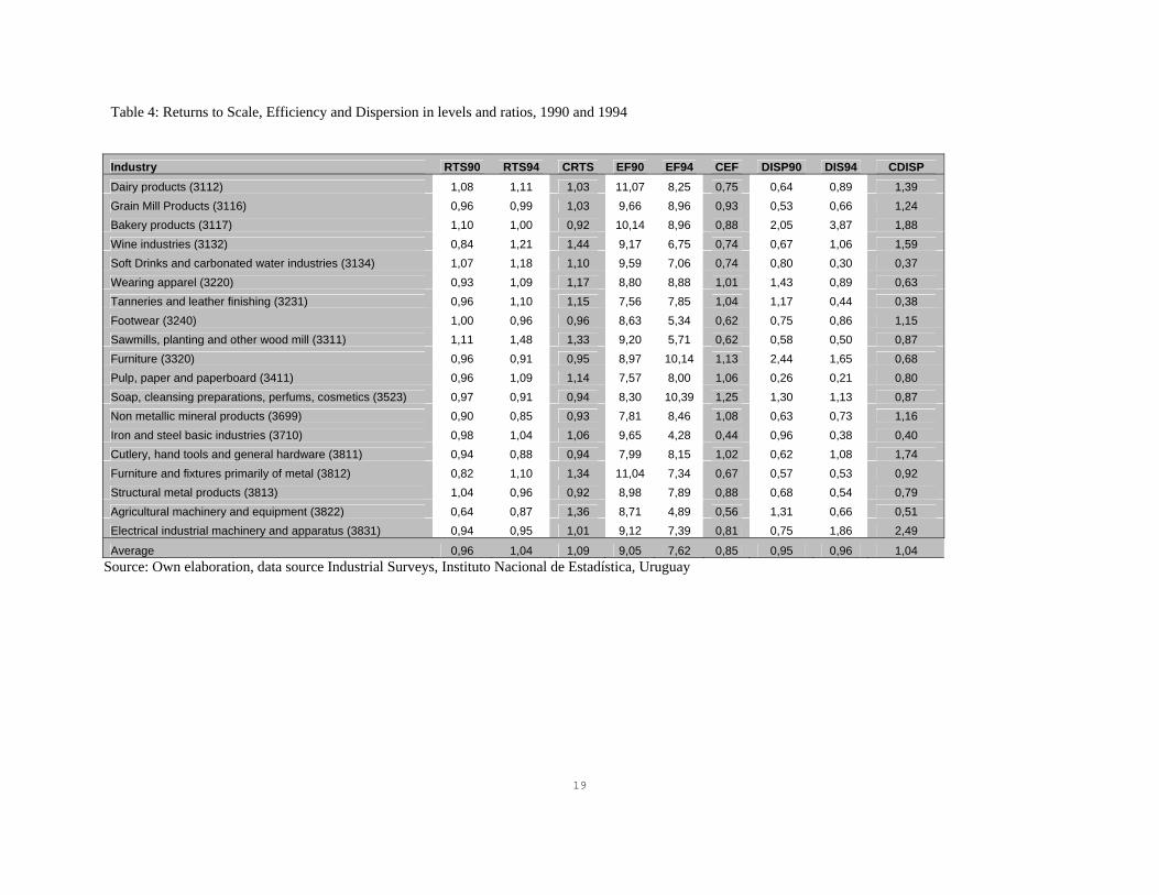
Working at a 4-digit ISIC code level we estimate a Cobb Douglas production function for 37 industries as we described earlier. We found that for 19 branches there were unitary returns to scale for both years. In Table 4 we present the estimates of returns to scale (RTS) for years, as well as the indicators of efficiency (EF) and dispersion (DISP) for these 19 branches and in ratios.

We found that for 7 out of 19 industries there was an increase in efficiency (37 % of the industries in the sub sample), the ratio of returns to scale decrease for 7 industries (37 % of the industries), while dispersion decrease for 11 industries (58 %). Nevertheless, the average values for these 19 industries show a decrease in efficiency, and an increase in the scale ratio and dispersion, contrary to our expectations. These results are in line with those obtained by Tybout et al. (1991) working for the Chilean manufacturing sector.

Then we calculate the Spearman’s rank correlation coefficient (Table 5). The trade variables tested were import penetration, nominal and weighted average rate of protection taken as ratios.

There is a negative and significant association between the return to scale ratio and average protection ratio, which implies that a decrease in protection is associated with decreasing returns to scale, contrary to our expectations. One possible explanation to these results is that there is idle installed capacity in the manufacturing industry. In this regard, a survey carried out by the Chamber of Industry in 1996 points out the existence of idle capacity over all for industries that process agricultural goods which in our case represent 10 out of the 19 branches considered in this work. So, it might be the case that the tariff reduction and the appreciation of domestic currency tend to reduce domestic production, and consequently increase idle capacity, reducing so efficiency and returns to scale. Also, as argued by Roberts and Tybout (1996) this result may be due to a countercyclical behaviour of productivity.

For the efficiency ratio we found a significant and negative relation with the scale ratio (-0.475**). The negative association between the ratios of efficiency and returns to scale means that gains in efficiency are associated with gains in economies of scale due to increasing returns. Nevertheless we found an unexpected positive association between the ratio of efficiency and the average and nominal protection ratio. These positive associations between efficiency and protection ratios show that the decrease in protection does not translate into increases in efficiency for the sample analyzed. Also we should keep in mind that estimation of scale and efficiency might be improved working with panel data, more flexible functional forms and correcting for mis-measurements in capital stock, as well as simultaneity and endogeneity in the estimates of returns to scale.

19

Table 4: Returns to Scale, Efficiency and Dispersion in levels and ratios, 1990 and 1994 Industry RTS90 RTS94 CRTS EF90 EF94 CEF DISP90 DIS94 CDISP Dairy products (3112) 1,08 1,11 1,03 11,07 8,25 0,75 0,64 0,89 1,39 Grain Mill Products (3116) 0,96 0,99 1,03 9,66 8,96 0,93 0,53 0,66 1,24 Bakery products (3117) 1,10 1,00 0,92 10,14 8,96 0,88 2,05 3,87 1,88 Wine industries (3132) 0,84 1,21 1,44 9,17 6,75 0,74 0,67 1,06 1,59 Soft Drinks and carbonated water industries (3134) 1,07 1,18 1,10 9,59 7,06 0,74 0,80 0,30 0,37 Wearing apparel (3220) 0,93 1,09 1,17 8,80 8,88 1,01 1,43 0,89 0,63 Tanneries and leather finishing (3231) 0,96 1,10 1,15 7,56 7,85 1,04 1,17 0,44 0,38 Footwear (3240) 1,00 0,96 0,96 8,63 5,34 0,62 0,75 0,86 1,15 Sawmills, planting and other wood mill (3311) 1,11 1,48 1,33 9,20 5,71 0,62 0,58 0,50 0,87 Furniture (3320) 0,96 0,91 0,95 8,97 10,14 1,13 2,44 1,65 0,68 Pulp, paper and paperboard (3411) 0,96 1,09 1,14 7,57 8,00 1,06 0,26 0,21 0,80 Soap, cleansing preparations, perfums, cosmetics (3523) 0,97 0,91 0,94 8,30 10,39 1,25 1,30 1,13 0,87 Non metallic mineral products (3699) 0,90 0,85 0,93 7,81 8,46 1,08 0,63 0,73 1,16 Iron and steel basic industries (3710) 0,98 1,04 1,06 9,65 4,28 0,44 0,96 0,38 0,40 Cutlery, hand tools and general hardware (3811) 0,94 0,88 0,94 7,99 8,15 1,02 0,62 1,08 1,74 Furniture and fixtures primarily of metal (3812) 0,82 1,10 1,34 11,04 7,34 0,67 0,57 0,53 0,92 Structural metal products (3813) 1,04 0,96 0,92 8,98 7,89 0,88 0,68 0,54 0,79 Agricultural machinery and equipment (3822) 0,64 0,87 1,36 8,71 4,89 0,56 1,31 0,66 0,51 Electrical industrial machinery and apparatus (3831) 0,94 0,95 1,01 9,12 7,39 0,81 0,75 1,86 2,49

Average 0,96 1,04 1,09 9,05 7,62 0,85 0,95 0,96 1,04 Source: Own elaboration, data source Industrial Surveys, Instituto Nacional de Estadística, Uruguay

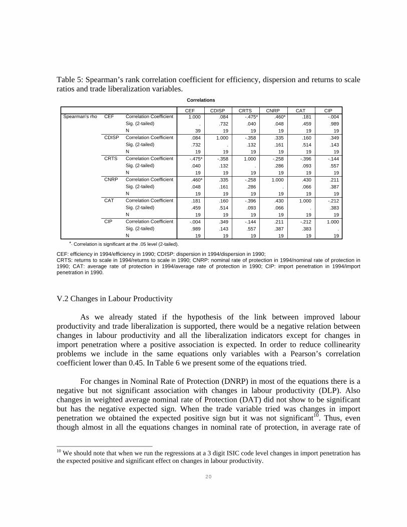
Table 5: Spearman’s rank correlation coefficient for efficiency, dispersion and returns to scale ratios and trade liberalization variables.

Correlations

1.000 .084 -.475* .460* .181 -.004. .732 .040 .048 .459 .989

39 19 19 19 19 19.084 1.000 -.358 .335 .160 .349.732 . .132 .161 .514 .143

19 19 19 19 19 19-.475* -.358 1.000 -.258 -.396 -.144.040 .132 . .286 .093 .557

19 19 19 19 19 19.460* .335 -.258 1.000 .430 .211.048 .161 .286 . .066 .387

19 19 19 19 19 19.181 .160 -.396 .430 1.000 -.212.459 .514 .093 .066 . .383

19 19 19 19 19 19-.004 .349 -.144 .211 -.212 1.000.989 .143 .557 .387 .383 .

19 19 19 19 19 19

Correlation CoefficientSig. (2-tailed)NCorrelation CoefficientSig. (2-tailed)NCorrelation CoefficientSig. (2-tailed)NCorrelation CoefficientSig. (2-tailed)NCorrelation CoefficientSig. (2-tailed)NCorrelation CoefficientSig. (2-tailed)N

CEF

CDISP

CRTS

CNRP

CAT

CIP

Spearman's rhoCEF CDISP CRTS CNRP CAT CIP

Correlation is significant at the .05 level (2-tailed).*.

CEF: efficiency in 1994/efficiency in 1990; CDISP: dispersion in 1994/dispersion in 1990; CRTS: returns to scale in 1994/returns to scale in 1990; CNRP: nominal rate of protection in 1994/nominal rate of protection in 1990; CAT: average rate of protection in 1994/average rate of protection in 1990; CIP: import penetration in 1994/import penetration in 1990. V.2 Changes in Labour Productivity

As we already stated if the hypothesis of the link between improved labour productivity and trade liberalization is supported, there would be a negative relation between changes in labour productivity and all the liberalization indicators except for changes in import penetration where a positive association is expected. In order to reduce collinearity problems we include in the same equations only variables with a Pearson’s correlation coefficient lower than 0.45. In Table 6 we present some of the equations tried.

For changes in Nominal Rate of Protection (DNRP) in most of the equations there is a negative but not significant association with changes in labour productivity (DLP). Also changes in weighted average nominal rate of Protection (DAT) did not show to be significant but has the negative expected sign. When the trade variable tried was changes in import penetration we obtained the expected positive sign but it was not significant10. Thus, even though almost in all the equations changes in nominal rate of protection, in average rate of

10 We should note that when we run the regressions at a 3 digit ISIC code level changes in import penetration has the expected positive and significant effect on changes in labour productivity.

20

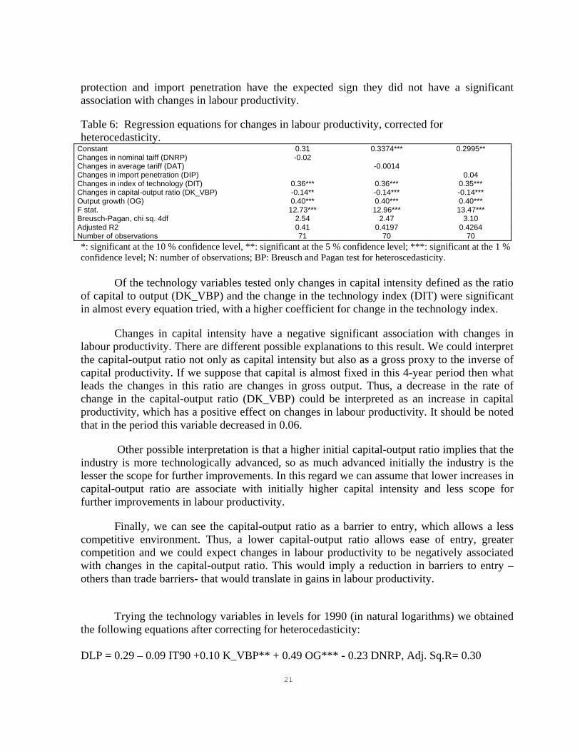
protection and import penetration have the expected sign they did not have a significant association with changes in labour productivity. Table 6: Regression equations for changes in labour productivity, corrected for heterocedasticity.

Constant 0.31 0.3374*** 0.2995** Changes in nominal taiff (DNRP) -0.02 Changes in average tariff (DAT) -0.0014 Changes in import penetration (DIP) 0.04 Changes in index of technology (DIT) 0.36*** 0.36*** 0.35*** Changes in capital-output ratio (DK_VBP) -0.14** -0.14*** -0.14*** Output growth (OG) 0.40*** 0.40*** 0.40*** F stat. 12.73*** 12.96*** 13.47*** Breusch-Pagan, chi sq. 4df 2.54 2.47 3.10 Adjusted R2 0.41 0.4197 0.4264 Number of observations 71 70 70 *: significant at the 10 % confidence level, **: significant at the 5 % confidence level; ***: significant at the 1 % confidence level; N: number of observations; BP: Breusch and Pagan test for heteroscedasticity.

Of the technology variables tested only changes in capital intensity defined as the ratio of capital to output (DK_VBP) and the change in the technology index (DIT) were significant in almost every equation tried, with a higher coefficient for change in the technology index.

Changes in capital intensity have a negative significant association with changes in labour productivity. There are different possible explanations to this result. We could interpret the capital-output ratio not only as capital intensity but also as a gross proxy to the inverse of capital productivity. If we suppose that capital is almost fixed in this 4-year period then what leads the changes in this ratio are changes in gross output. Thus, a decrease in the rate of change in the capital-output ratio (DK_VBP) could be interpreted as an increase in capital productivity, which has a positive effect on changes in labour productivity. It should be noted that in the period this variable decreased in 0.06.

Other possible interpretation is that a higher initial capital-output ratio implies that the industry is more technologically advanced, so as much advanced initially the industry is the lesser the scope for further improvements. In this regard we can assume that lower increases in capital-output ratio are associate with initially higher capital intensity and less scope for further improvements in labour productivity.

Finally, we can see the capital-output ratio as a barrier to entry, which allows a less competitive environment. Thus, a lower capital-output ratio allows ease of entry, greater competition and we could expect changes in labour productivity to be negatively associated with changes in the capital-output ratio. This would imply a reduction in barriers to entry –others than trade barriers- that would translate in gains in labour productivity.

Trying the technology variables in levels for 1990 (in natural logarithms) we obtained

the following equations after correcting for heterocedasticity: DLP = 0.29 – 0.09 IT90 +0.10 K_VBP** + 0.49 OG*** - 0.23 DNRP, Adj. Sq.R= 0.30

21

DLP = 0.38*** – 0.09 IT90 +0.09 K_VBP* + 0.48 OG***- 0.07 DAT, Adj. Sq.R= 0.30 DLP = 0.40*** – 0.07 IT90 +0.096 K_VBP* + 0.48OG***+0.05 DIP, Adj. Sq.R2= 0.31

Thus, there is a positive association among the initial level of capital-output ratio (K_VBP) and changes in labour productivity. The positive sign might be interpreted as if the technological dynamism of capital intensive industries outweighs the negative effect of capital intensity as a barrier to entry. From the above equations we observe a negative though not significant sign of the index of technology when we take the variable in levels for 1990. Therefore, an initially lower index of technology (IT) implies a greater scope for catching up and improvements in productivity.

Changes in the index of technology (DIT) have a positive and significant effect on changes in labour productivity. In the period, the technology index increases in 0.11. This increase means that there was a decrease in the gap among the firm with highest productivity and the others firms at the industry level. Therefore, there is a positive association between improvements in the technology index and changes in labour productivity.

Of the market structure variable changes in concentration (DHC) have a negative not significant effect on changes in labour productivity11.

To have a better insight of the effects of concentration we split the sample in high concentrated and less concentrated industries. We define as high concentration those industries that have a Herfindhal index greater than the average value for 1990 (H=0.09). We then studied the more concentrated industries. For industries with high concentration we have to restrict the analysis to output growth and the trade variable as explanatory variables due to the increase in the correlation among variables when we worked on this sub-sample. We obtained the following equations:

DLP= 0.14 + 0.44 OG** - 0.36 DNRP, Adj.Sq.R.=14.82, N=15, Chi sq(2)=1.78 DLP= 0.26*** + 0.45 OG*** - 0.16 DAT*, Adj.Sq.R=32.79, N=15, Chi sq(2)=1.65 DLP= 0.31*** + 0.39 OG*** + 0.066 DIP*, Adj.Sq.R=21.21, N=15; Chi sq(2)=1.52

Thus, for the more concentrated industries there is a significant negative effect of changes in weighted average tariff (DAT) on changes in labour productivity, while changes in import penetration have the positive and significant expected sign. These results are showing that for more concentrated industries liberalisation has a positive impact on labour productivity. 11 Working at a 3 digit ISIC code level we found that changes in concentration have a significant and negative effect on changes in labour productivity.

22

Output growth was always positively significant, and with a relatively high coefficient, pointing out the existence of dynamic scale effects associated with labour productivity improvements.

To sum up, for changes in labour productivity we found that generally changes in the trade variable have the expected positive sign though not significant. Nevertheless, for more concentrated branches we found the effect of trade variables become relevant with a significant negative effect of changes in average protection and a positive effect of increased import competition and the reduction in effective protection. Output growth was an important variable having a significant positive effect on productivity improvements.

In addition, changes in the technology index and capital-output ratio have a significant

effect on changes in labour productivity. While an increase in the index of technology has a significant positive impact on productivity and changes in capital-output ratio a negative significant effect. Thus, it seems that for the short period analyzed technology and market structure variables are relatively more important than trade variables in explaining gains in labour productivity. Nevertheless, liberalisation shows a positive impact in more concentrated industries. 3. Changes in Price Cost Margins (DPCM)

In Table 7 we present the equations when we take all the variables in rates of changes for the branches at 4-digit ISIC code level. Since price-cost margins and its changes is highly heterosckedastic we corrected the results using White’s covariance matrix.

If the hypothesis on the link between trade liberalization and performance is to be confirmed we will expect a positive association among between in price cost margins and changes in nominal, average and effective protection, and a negative association with changes in import penetration and exports growth.

Changes in nominal rate of protection have a positive but not significant effect on changes in price cost margins for all the equations tried. On the contrary changes in weighted average nominal protection (DAT) have an unexpected negative sign though they were not significant.

Also changes in import penetration (DIP) have an unexpected positive and significant effect on changes in mark-ups. Thus, the increase in imports does not translate in a reduction in marks ups12. We could think that the entry of imports is higher in those industries with initially higher marks up, and that there is a time lag before firms react adjusting prices to

12 When we run the regression at a 3 digit ISIC code level we found that changes in import penetration have not a significant effect and its sign changed according to the rest of the other explanatory variables, possibly due to multicollinearity problems.

23

increased import competition. Furthermore, Weiss and Jayanthakumaran (1995) and de Melo and Urata (1984) found similar results between changes in price cost margins and import penetration. Their explanation is that this is the result of monopolistic control over the distribution sector, so in spite of higher import penetration, higher mark ups on those goods are set by distributors which at its time allows higher mark ups by domestic producers of import competing goods. In this regard a monopolistic distribution sector might have contributed to a slow reduction in mark ups. This explanation might apply quite well for the Uruguayan case due to the oligopolistic structure of the importer and the distribution sectors in the country, as well in manufacturing industry.

Other possible interpretation is that it could be the case that when firms set prices they do not know a priori which will be the actual competition from imports. Perhaps the relevant variable that firms take into account to set prices is past import competition. To test this we included lagged import penetration13 and it showed a negative sign though not significant14.

Nevertheless, we should keep in mind that macroeconomic variables, such as price stabilization and the reactivation of the domestic market might be affecting this result.

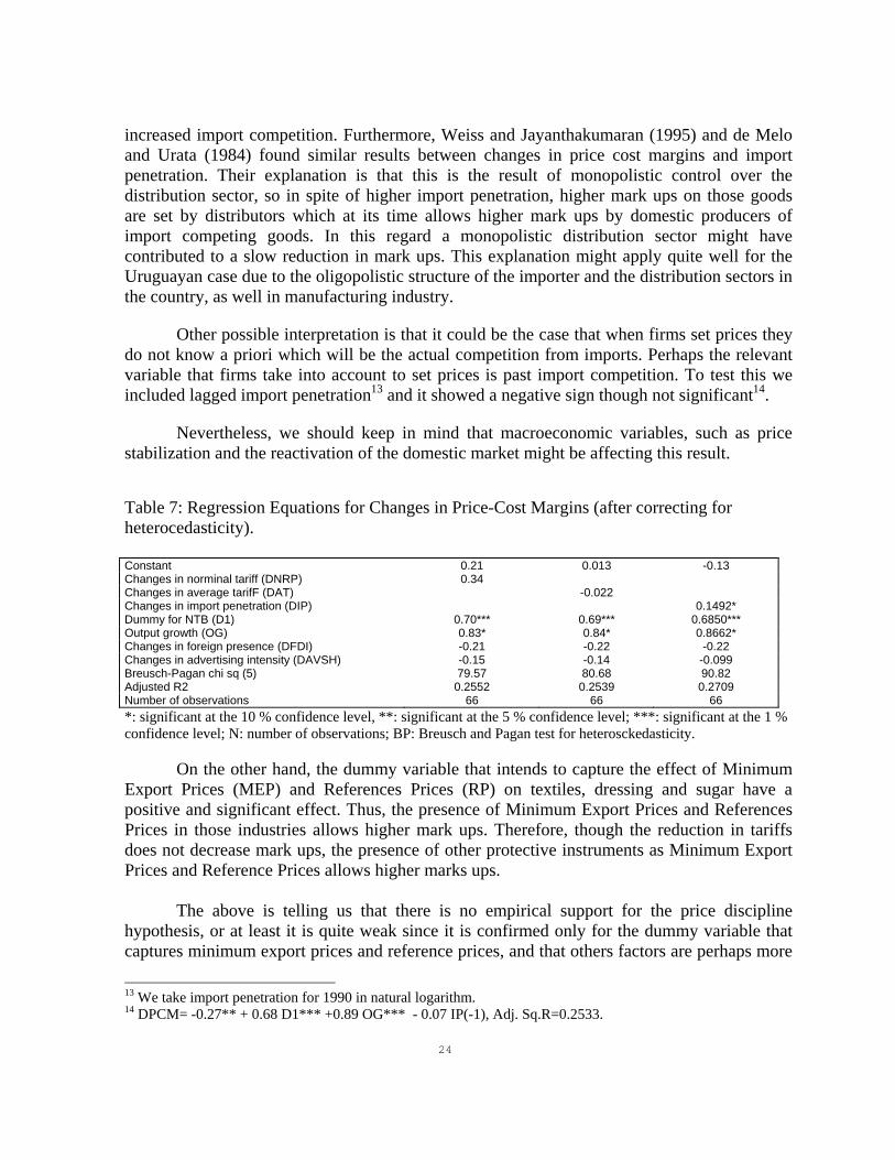
Table 7: Regression Equations for Changes in Price-Cost Margins (after correcting for heterocedasticity). Constant 0.21 0.013 -0.13 Changes in norminal tariff (DNRP) 0.34 Changes in average tarifF (DAT) -0.022 Changes in import penetration (DIP) 0.1492* Dummy for NTB (D1) 0.70*** 0.69*** 0.6850*** Output growth (OG) 0.83* 0.84* 0.8662* Changes in foreign presence (DFDI) -0.21 -0.22 -0.22 Changes in advertising intensity (DAVSH) -0.15 -0.14 -0.099 Breusch-Pagan chi sq (5) 79.57 80.68 90.82 Adjusted R2 0.2552 0.2539 0.2709 Number of observations 66 66 66 *: significant at the 10 % confidence level, **: significant at the 5 % confidence level; ***: significant at the 1 % confidence level; N: number of observations; BP: Breusch and Pagan test for heterosckedasticity.

On the other hand, the dummy variable that intends to capture the effect of Minimum Export Prices (MEP) and References Prices (RP) on textiles, dressing and sugar have a positive and significant effect. Thus, the presence of Minimum Export Prices and References Prices in those industries allows higher mark ups. Therefore, though the reduction in tariffs does not decrease mark ups, the presence of other protective instruments as Minimum Export Prices and Reference Prices allows higher marks ups.

The above is telling us that there is no empirical support for the price discipline hypothesis, or at least it is quite weak since it is confirmed only for the dummy variable that captures minimum export prices and reference prices, and that others factors are perhaps more

13 We take import penetration for 1990 in natural logarithm. 14 DPCM= -0.27** + 0.68 D1*** +0.89 OG*** - 0.07 IP(-1), Adj. Sq.R=0.2533.

24

important to explain higher marks ups that the reduction in trade protection. Besides, we should keep in mind the high heterogeneity among firms that belong to the same industry (Tansini, et al., 1998; Tybout, 2001) and that we are taking average values at the branch level which might be biasing the results15. We intend we deal with this issue in future work working with plant level data and panel methodologies.

Of the market structure variables tested we found that the changes in advertising intensity (DAVSH) and in foreign presence (DFDI) have a negative and significant effect implying that those industries that increase advertising intensity, and so more differentiated products have a lower growth in price cost margin. We tried foreign presence (FDI) and advertising intensity (ADVSH) in levels and logarithms for 1990. The best-fit equation was the following after correcting for White’s robust covariance matrix: DPCM=--1.7* +1.0 OG*** –0.62 D1***- 0.17 ADVSH90 + 0.21 DIP*** Adj Sq.R.=0.3441, B-P chi sq.=59.847,N=66.

Thus, though advertising intensity is not significant it has the expected negative sign, which implies a negative association between an initial higher level of advertising intensity and changes in price cost margins. On the other hand, the change in import penetration is again positive and significant.

Output growth (OG) showed a positive and significant effect in most of the cases reflecting dynamic economies of scale that translate into higher price cost margins.

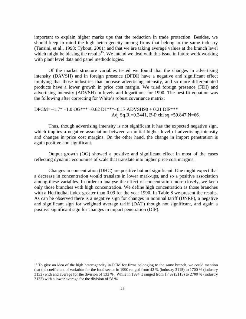
Changes in concentration (DHC) are positive but not significant. One might expect that a decrease in concentration would translate in lower mark-ups, and so a positive association among these variables. In order to analyse the effect of concentration more closely, we keep only those branches with high concentration. We define high concentration as those branches with a Herfindhal index greater than 0.09 for the year 1990. In Table 8 we present the results. As can be observed there is a negative sign for changes in nominal tariff (DNRP), a negative and significant sign for weighted average tariff (DAT) though not significant, and again a positive significant sign for changes in import penetration (DIP).

15 To give an idea of the high heterogeneity in PCM for firms belonging to the same branch, we could mention that the coefficient of variation for the food sector in 1990 ranged from 42 % (industry 3115) to 1700 % (industry 3132) with and average for the division of 132 %. While in 1994 it ranged from 17 % (3113) to 2700 % (industry 3132) with a lower average for the division of 58 %.

25

Table 8: Regression Equations for changes in Price-Cost Margins for more concentrated branches using White’s covariance matrix Constant -1.26 -0.23 -0.27 Changes in nominal tariff (DNRP) -2.11 Changes in import penetration (DIP) 0.34*** Changes in average tariff (DAT) -0.43*** Output growth (OG) 1.14* 1.16* 0.91* Breusch-Pagan chi sq (3df) 1.58 0.82** 2.35 Adjusted R2 13.30 34.9 27.93 Number of observations 15 15 15 *: significant at the 10 % confidence level, **: significant at the 5 % confidence level; ***: significant at the 1 % confidence level; N: number of observations; BP: Breusch and Pagan test for heterosckedasticity. When we consider changes in efficiency as an explanatory variable we found that it has a positive and significant impact on changes in price cost margins. We obtained the following equation using White’s covariance matrix: DPCM= 0.33 - 0.018 DIP + 0.12 D1* + 1.23 DEF* N=17, R sq adj=0.3015, B-P chi-sq(5)=8.6266

Also we tried changes in labour productivity and efficiency finding a positive and significant effect on PCM. Therefore, higher labour productivity and efficiency do not translate into lower prices but in higher mark ups. The estimated equations are the following: DPCM = 0.36 + 1.02 DNRP +0.43 D1*** -0.19 DADVSH +0.63 DLP***, Rsq.adj.=15.17, B-P chi sq.(4)=14.90; DPCM = - 0.25 + 0.41 DAT+0.42 D1** -0.19 DAVSH +0.65 DLP***, Rsq.adj.=13.96, B-P chi sq.(4)=11.34; DPCM = - 0.33+ 0.05 DIP+0.40 D1*** -0.17 DAVSH**+0.65 DLP***, Rsq.adj.=14.26, B-P chi sq.(4)=15.40;

Summing up, when the dependent variables are changes in price-cost margins, results are even weaker. Except for the dummy variable intended to capture the effect of Minimum Export Prices and Reference Prices the results do not confirm the price discipline hypothesis, at least for the short period analysed. Output growth proved to be a relevant variable in explaining higher mark ups.

Nevertheless, we should keep in mind different aspects that could be affecting our results. One is that our model is not capturing other variables as price stabilization, the reactivation of domestic markets, the appreciation of domestic currency, as well as other industrial and fiscal policies that are at work. Also there are other important sectors as the distribution sector that has kept its monopoly power in the period analyzed, and the period analysed might be too short to capture fully the effect of liberalisation. Finally, we should point out the high variability of PCM for firms belonging to the same industry and that we are taking average values which could be affecting the results.

26

Conclusions

As many other empirical works, our analysis is far from conclusive, though it provided some weak evidence between changes in returns to scale, labour productivity and price-cost-margins and some measures of change in trade policy, as well as technology and market structure variables.

For returns to scale, we did not find that trade liberalization brought gains in scale economies. On the contrary we found that the reduction in average rate of protection has a negative effect on increasing returns. As we have already noted for changes in labour productivity we have found that changes in nominal rate, average rate and import penetration have the expected sign though not significant.

It is sometimes hypothesized that there is a varying degree of response to trade liberalization depending on the initial concentration in the branch. It is expected that a higher concentration provide a greater scope for efficiency gains in response to stronger import competition. This has some support in our results since when the sample is split into high and low concentrated branches changes in average rate and effective rate of protections have the expected negatively significant sign for more concentrated branches.

Output growth is one of the most significant variables with a higher coefficient. General macroeconomic conditions as well as branch specific factors will determine it. Also we found a positively significant correlation Pearson’s coefficient between OG and changes in nominal rate of protection (0.22 at a 5% level) Changes in the index of technology have a positive significant effect on changes in LP, implying that when firms move towards the best practice there are gains in LP. While changes in capital output ratio have a negative impact on LP growth. These results point out the importance of technological and market structure variables in explaining productivity growth as well as a weak effect of trade variables.

When the dependant variable considered was changes in price cost margins we found that the only trade significant variable with the expected positive sign was a dummy that captures the effects of Minimum Exports Prices and References Prices (D1). For the rest of the trade variables considered signs were those expected though not significant, except for changes in import penetration, which presented a significant coefficient with unexpected positive sign. Nevertheless lagged import penetration showed the negative expected sign though it was not significant. The positive impact of greater import penetration associated with higher mark ups were found also in other empirical studies and could be a result of monopolistic distribution structures as we have already noted.

One of the more important structure variables is OG, being always positive and significant.

27

Also changes in labour productivity and efficiency proved to have a significant positive effect on changes in PCM. So higher productivity and efficiency do not pass to consumers through lowers price but are kept by producers as higher profits. This could be explained as the result of the non competitive structure, not only of manufacturing industries, but also of other keys sectors as the distribution one.

As we already noted, it is clear that changes in performance are due to many factors other than trade liberalization. Macroeconomic conditions as appreciation of the domestic currency, price stabilization and the reactivation of the domestic demand, as well as specific industrial and fiscal policies that are at work and possibly influencing the results. Also the period analyzed might be too short to capture fully the effect of liberalization.

Full explanations of changes in performance must identify causes of output and demand changes at the branch level. This will imply and analysis of specific demand conditions and supply constraints. Trade liberalization is just one element of the analysis whose short run effects appear relatively weak but positive. Thus, we can not expect that trade liberalization was the only instrument to improve performance of the industrial sector of developing countries, and, as the results show, there is still a role for policies aimed to promote competition and technological change.

28

References

Arimon G. Y Romaniello, G., 1994: “Factores determinantes de la rentabilidad en la industria uruguaya”, mimeo, Departamento de Economía, Facultad de Ciencias Sociales, Universidad de la República. Baier, Scott L., Gerald P. Dwyer Jr. and Robert Tamura, 2002: “Crescimento e Productividade no Brasil: o que nos diz o Registro de Longo Prazo.” Seminarios DINAC N’ 52 IPEA, Rio de Janeiro. Berndt, Ernst,1991, Econometric Analysis, Mac Millan, New York. Bhagwatti, Jagdish, “Export-Promoting Trade Strategy: Issues and Evidence”, The World Bank Research Observer, Vol. 3, 1988, pp. 27-57. Carella, A., Domingo, R., Pastori, H., Rossi, M., Tansini, R., 1998: “El Sector Industrial: Perspectivas ante la Apertura y la Integración”, mimeo, Departamento de Economía, Facultad de Ciencias Sociales, Universidad de la República. De Melo J. And David Roland-Holst, 1988: “Industrial Organization and Trade Liberalization: Evidence from Korea”, in Empirical Studies of Commercial Policy, ed. By R. E. Baldwin, pp. 287-311. Dutz, Mark A., 1991: “Firm Output Adjustment to Trade Liberalization, Theory and Application to the Moroccan Experience, Working Papers, WPS 602, The World Bank. Fernandes, Ana, 2001: “Trade Policy, Trade Volumenes and Plant Level Productivity in Colombian Manufacturing Industries”, Department of Economics Yale University. Greene, W. H. (1980), Econometric Analysis, Mac Millan, New York. Harrison, Ann E., 1990, “Productivity, Imperfect Competition and Trade Liberalization in Cote d’Ivoire, Working Papers, WPS 451, The World Bank. IDB, 2001. “Competitiveness: The Business of Growth”, Economic and Social Progress in latin America. Washington D.C. Inter-American Development Bank.

29

Katayama, Hajime, Lu Shihua and James Tybout, 2003, “Why Plant-Level Productivity Studies are Often Misleading, and an Alternative Approach to Inference. Pnnyslvania State University. Kokko, A.; Tansini R. & Zejan M. (1996): “Local Technological Capability and Productivity Spillovers from FDI in the Uruguayan Manufacturing Sector”, Journal of Development Studies, 32. Loyama, Norman, P. Fajnzylber and C. Calderon , 2002, “Economic Growth in Latin America and the Caribbean. Stylized facts, explanations and forecasts. World Bank, Washington D.C. Lopez-Cordova , Ernesto, and Mauricio Mesquita Moreira,2003, “Regional Integration and Productivity: The Experiences of Brazil and Mexico”, INTAL-ITD-STA, Working Paper 14. Macadar, L.; 1995: “La Política Arancelaria de Uruguay y las Negociaciones en el Marco del MERCOSUR”, mimeo, Ministerio de Economía, Montevideo, Uruguay. Melitz, Marc J., 2002, “The Impact of Trade on Intra-Industry Reallocations and Aggregate Industry Productivity”. Harvard University, Departments of Economics, March. Muendler, Marc-Andreas, 2002, “Trade, Technology and Productivity: A Study of Brazilian Manufacturers, 1986-1998”, University of California, Berkley, mimeo. Pack; H.; 1988:“Industrialization and Trade”, in H. Chenery and T. Srinivasan, Handbook of Development Economics, Amsterdam, North Holland. Pratten, C. F., 1971: Economies of scale in manufacturing industry, Cambridge University Press. Pacvnick, Nina (2000) “Trade Liberalization, Exit and Productivity Improvements: Evidence form Chilean Plants”, Department of Economics, Dartmouth College. Roberts, M. C. and James Tybout , 1996 (eds.) Industrial Evolution in Developing Countries. New York: Oxford University Press. Rodrik, D. (1988ª): “Imperfect Competition, Scale Economies and Trade Policy in Developing Countries”, mimeo, Harvard University. Rodrik, Dani, 1992: “Closing the Productivity Gap: Does Liberalisation Really Help?, in Gerald K. Hellener (ed.), Trade Policy Industrialization and Development: New Perspectives, Oxford: Clarendon Press. Scherer, F., 1980, Industrial Market Structure and Economic Performance, Chicago, IL: Rand Mac Nally.

30

Tansini, R. & Triunfo P., 1998: “Eficiencia Técnica y Apertura Externa en cuatro ramas industriales”, Departamento de Economía, FCS, Documento de Trabajo Nº 4/98, Montevideo, Uruguay. Tansini, R. & Triunfo P., 1998: “Eficiencia Técnica y Apertura Externa en el Sector Manufacturero Uruguayo”, Departamento de Economía, FCS, Documento de Trabajo Nº 9/98, Montevideo, Uruguay. Tansini, R. & Triunfo P., 1998: “Cambio Tecnológico y Productividad en las empresas industriales uruguayas”, Departamento de Economía, FCS, Documento de Trabajo N 12/98, Montevideo, Uruguay. Tybout, James, 2001, Plant and Firm-Level Evidence on New Trade Theories. In Handbook of International Economics, ed. James Harrigan. Vol 38 Basil-Blackwell. Tybout J., M. D. Westbrook, “Scale Economies as a Source of Efficiency Gains”, in Industrial Evolution in Developing Countries, Micro Patterns of Turnover, Productivity, and Market Structure, 104-141, Oxford University Press. Tybout, J., 1991: “Researching the Trade-Productivity Link”, World Bank, Working Paper RPO 674. Tybout, J., Jaime de Melo and Vittorio Corbo, 1990: “The Effects of Trade Reform on Scale and Technical Efficiency, new Evidence from Chile”, Working Papers, The World Bank. Tybout, J. R., 1992: “Making noisy data sing, Estimating production technologies in developing countries”, Journal of Econometrics, 53, North Holland. Vaillant, M., 1998: “Protección Administrada en el Uruguay: el caso de los precios regulados del comercio exterior”, versión preliminar, mimeo, Departamento de Economía, F.C.S., Universidad de la Republica, Montevideo, Uruguay. Weiss, John, 1992ª: “Trade Liberalization in Mexico in the 1980s: Concepts, Measures and Short-Run Effects”, Weltwirtschaftliches Archiv, 128(4): 711-25. Weiss, John, 1992b: “Trade Policy Reform and Performance in Manufacturing Mexico 1975-1988”; Journal of Development Studies 29(1): 1-23. Weiss, J. And k. Jayanthakumaran, 1995: “Trade Reform and Manufacturing Performance: Evidence from Sri Lanka, 1978-89; Development Policy Review, Vol. 13.

31

APPENDIX 1: Evolution of Nominal and Weighted Average Rate of Protection, 1990-1994.- INDUSTRY NRP90 NRP94 % VAR. AT90 AT94 % VAR.

3111 27,33 16,12 -41,02 20,15 13,79 -31,56 3112 27,50 16,68 -39,35 19,59 17,38 -11,28 3113 35,73 19,72 -44,81 37,88 19,76 -47,84 3114 28,20 17,79 -36,91 26,20 16,60 -36,64 3115 29,19 14,44 -50,53 23,82 13,01 -45,38 3116 31,29 18,33 -41,42 24,70 15,81 -35,99 3117 30,83 17,00 -44,86 36,10 18,62 -48,42 3118 34,35 15,69 -54,32 33,33 0,95 -97,15 3119 38,33 19,48 -49,18 33,41 19,31 -42,20 3121 32,83 17,83 -45,69 25,45 12,96 -49,08 3122 25,00 15,00 -40,00 25,00 15,00 -40,00 3132 38,46 20,00 -48,00 39,67 20,00 -49,58 3133 40,00 20,00 -50,00 40,00 20,00 -50,00 3134 32,73 17,51 -46,50 22,76 14,98 -34,18 3140 33,75 18,50 -45,19 29,59 18,15 -38,66 3211 31,52 18,22 -42,20 30,18 19,02 -36,98 3212 38,37 19,72 -48,61 39,51 19,99 -49,41 3213 38,89 19,41 -50,09 39,98 19,96 -50,08 3214 38,81 20,00 -48,47 39,14 20,00 -48,90 3219 30,00 15,78 -47,40 33,29 18,10 -45,63 3220 36,67 19,69 -46,30 38,54 19,86 -48,47 3231 15,00 6,00 -60,00 15,00 6,00 -60,00 3233 32,12 18,60 -42,09 36,04 19,45 -46,03 3240 39,38 20,00 -49,21 40,00 20,00 -50,00 3311 36,60 19,35 -47,13 31,54 19,76 -37,35 3312 39,71 20,00 -49,63 40,00 20,00 -50,00 3319 34,43 18,75 -45,54 38,11 19,99 -47,55 3320 36,15 20,00 -44,67 39,23 20,00 -49,02 3411 30,39 16,10 -47,02 27,08 15,87 -41,40 3412 33,33 19,44 -41,67 39,54 20,00 -49,42 3419 30,63 16,47 -46,23 18,04 8,65 -52,05 3420 32,60 17,46 -46,44 36,57 19,07 -47,85 3511 18,94 9,73 -48,63 17,52 7,94 -54,68 3512 30,59 16,91 -44,72 27,79 15,37 -44,69 3513 26,95 13,02 -51,69 17,69 8,18 -53,76 3521 30,64 17,22 -43,80 33,16 18,99 -42,73 3522 23,74 12,65 -46,71 23,09 12,82 -44,48 3523 31,56 18,59 -41,10 26,73 18,03 -32,55 3529 26,69 14,62 -45,22 21,70 13,08 -39,72 3540 24,16 14,94 -38,16 19,04 17,40 -8,61 3551 33,10 18,16 -45,14 38,02 19,45 -48,84 3559 32,53 17,03 -47,65 29,72 14,98 -49,60

32

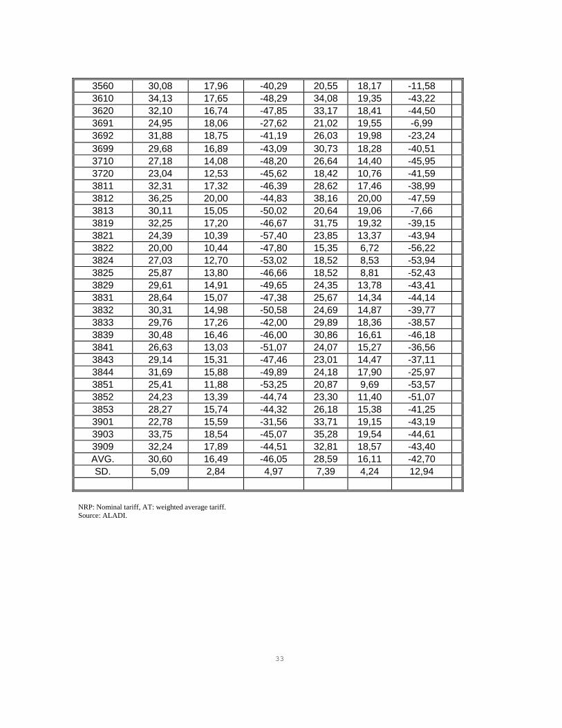
3560 30,08 17,96 -40,29 20,55 18,17 -11,58 3610 34,13 17,65 -48,29 34,08 19,35 -43,22 3620 32,10 16,74 -47,85 33,17 18,41 -44,50 3691 24,95 18,06 -27,62 21,02 19,55 -6,99 3692 31,88 18,75 -41,19 26,03 19,98 -23,24 3699 29,68 16,89 -43,09 30,73 18,28 -40,51 3710 27,18 14,08 -48,20 26,64 14,40 -45,95 3720 23,04 12,53 -45,62 18,42 10,76 -41,59 3811 32,31 17,32 -46,39 28,62 17,46 -38,99 3812 36,25 20,00 -44,83 38,16 20,00 -47,59 3813 30,11 15,05 -50,02 20,64 19,06 -7,66 3819 32,25 17,20 -46,67 31,75 19,32 -39,15 3821 24,39 10,39 -57,40 23,85 13,37 -43,94 3822 20,00 10,44 -47,80 15,35 6,72 -56,22 3824 27,03 12,70 -53,02 18,52 8,53 -53,94 3825 25,87 13,80 -46,66 18,52 8,81 -52,43 3829 29,61 14,91 -49,65 24,35 13,78 -43,41 3831 28,64 15,07 -47,38 25,67 14,34 -44,14 3832 30,31 14,98 -50,58 24,69 14,87 -39,77 3833 29,76 17,26 -42,00 29,89 18,36 -38,57 3839 30,48 16,46 -46,00 30,86 16,61 -46,18 3841 26,63 13,03 -51,07 24,07 15,27 -36,56 3843 29,14 15,31 -47,46 23,01 14,47 -37,11 3844 31,69 15,88 -49,89 24,18 17,90 -25,97 3851 25,41 11,88 -53,25 20,87 9,69 -53,57 3852 24,23 13,39 -44,74 23,30 11,40 -51,07 3853 28,27 15,74 -44,32 26,18 15,38 -41,25 3901 22,78 15,59 -31,56 33,71 19,15 -43,19 3903 33,75 18,54 -45,07 35,28 19,54 -44,61 3909 32,24 17,89 -44,51 32,81 18,57 -43,40 AVG. 30,60 16,49 -46,05 28,59 16,11 -42,70 SD. 5,09 2,84 4,97 7,39 4,24 12,94

NRP: Nominal tariff, AT: weighted average tariff. Source: ALADI.

33

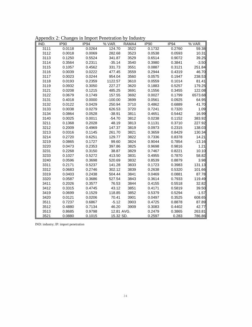
34

Appendix 2: Changes in Import Penetration by Industry

IND: industry; IP: import penetration

IND. IP90 IP94 % VAR. RAMA4 IP90 IP94 % VAR. 3111 0.0118 0.0264 124.70 3522 0.1732 0.2760 59.383112 0.0018 0.0069 282.68 3523 0.0538 0.0593 10.313113 0.1250 0.5524 341.87 3529 0.6514 0.9072 39.253114 0.3564 0.2311 -35.14 3540 0.3980 0.3841 -3.503115 0.1057 0.4562 331.73 3551 0.0887 0.3121 251.843116 0.0039 0.0222 477.45 3559 0.2944 0.4319 46.703117 0.0023 0.0244 954.04 3560 0.0575 0.1947 238.533118 0.0193 0.2359 1122.57 3610 0.0559 0.1014 81.413119 0.0932 0.3050 227.27 3620 0.1883 0.5257 179.253121 0.0208 0.1215 485.25 3691 0.1556 0.3455 122.083122 0.0679 0.1749 157.55 3692 0.0027 0.1799 6573.683131 0.4018 0.0000 -100.00 3699 0.0561 0.0925 64.953132 0.0122 0.0429 250.94 3710 0.4862 0.6889 41.703133 0.0038 0.0279 626.53 3720 0.7241 0.7320 1.093134 0.0864 0.0528 -38.91 3811 0.4651 0.5442 16.993140 0.0025 0.0011 -54.70 3812 0.0238 0.1152 383.923211 0.1368 0.2028 48.19 3813 0.1131 0.3710 227.923212 0.2009 0.4969 147.37 3819 0.0973 0.2315 138.033213 0.0316 0.1145 261.70 3821 0.3659 0.8429 130.343214 0.2720 0.6251 129.77 3822 0.7336 0.8378 14.213219 0.0865 0.1727 99.60 3824 0.9044 0.7854 -13.163220 0.0473 0.2353 397.86 3825 0.9698 0.9816 1.213231 0.2268 0.3150 38.87 3829 0.7467 0.8221 10.103233 0.1027 0.5272 413.50 3831 0.4955 0.7870 58.823240 0.0596 0.3698 520.69 3832 0.8539 0.8879 3.983311 0.2171 0.5237 141.28 3833 0.1723 0.3983 131.133312 0.0683 0.2746 302.12 3839 0.2638 0.5320 101.663319 0.0403 0.2438 504.44 3841 0.0469 0.0881 87.783320 0.0587 0.3686 527.54 3843 0.3614 0.7933 119.493411 0.2026 0.3577 76.53 3844 0.4155 0.5518 32.823412 0.3315 0.4745 43.12 3851 0.4171 0.5819 39.503419 0.0699 0.1529 118.85 3852 0.5379 0.5294 -1.573420 0.0121 0.0206 70.41 3901 0.0497 0.3525 608.653511 0.7237 0.6867 -5.12 3903 0.4725 0.8878 87.893512 0.4880 0.7134 46.20 3909 0.3083 0.4402 42.773513 0.8685 0.9798 12.81 AVG. 0.2479 0.3865 263.813521 0.0880 0.1015 15.32 SD. 0.2597 0.283 786.86