RESEARCH P

GRADUATE SCH

STANFORD

RESEARCH P

Financial Analysts and

MARY EStanford

AMY P.Harvard

Apri

APER NO. 1693

the Pricing of Accruals

. BARTH University

HUTTON University

APER SERIES

OOL OF BUSINESS

UNIVERSITY

l 2001

Research Paper No. 1693

Financial Analysts and the Pricing of Accruals

Mary E. Barth

Graduate School of Business Stanford University

Amy P. Hutton

Graduate School of Business Harvard University

April 2001

Abstract We test predictions relating to the role of financial analysts in aiding investors’ assessment of the different valuation implications of the cash flow and accrual components of earnings. First, we examine whether analysts revise their forecasts of future earnings in anticipation of predictable accrual reversals. Then, we examine whether share prices reflect predictable accrual reversals differently depending on analyst activity. Our findings suggest that analysts act as sophisticated information intermediaries in that some analysts are able to identify firms with less persistent accruals. However, share prices do not reflect the information conveyed by analyst forecast revisions. Rather, investors appear to expect the same persistence in earnings, regardless of its cash flow and accrual components and regardless of analyst activity, until the accruals reverse. Thus, incorporating information from analyst activity substantially improves short-tem returns to an accrual-based trading strategy.

________________________ Correspondence: Mary E. Barth, Stanford University, Graduate School of Business, Stanford, CA 94305, Tel. (650) 723-8536, Fax. (650) 725-0468, fbarth@leland.stanford.edu. Amy Hutton, Harvard University, Graduate School of Business, Boston, MA 02163, Tel (617) 495-6375, Fax (617) 496-7363, ahutton@hbs.edu. We appreciate helpful comments and suggestions from Mark Bradshaw, Greg Miller, S.P. Kothari, Richard Sloan, and participants at the 1999 Stanford Accounting Summer Camp and the 2000 AAA Annual Meetings. We also appreciate funding by the Financial Research Initiative and the GSB Faculty Trust of the Stanford University Graduate School of Business, and Division of Research, Harvard Business School. We also thank I/B/E/S for use of its analyst data and Chris Allen, Radhika Ashok, Sarah Eriksen, Philip Joos, and Yulin Long for research assistance.

1. Introduction

This study tests whether differences in the persistence of cash flows and accruals are

reflected more accurately and more quickly in share prices of firms with more active financial

analysts. The motivation for the study is to enhance our understanding of the role of information

intermediaries, specifically financial analysts, in aiding investors’ assessment of the valuation

implications of accounting data. We focus on the cash flow and accrual components of earnings

because prior research finds that investors fail to anticipate predictable differences in their

persistence (Sloan [1996], Xie [2000]), which are relevant to investors in assessing firm value

(Dechow [1994], Ohlson [1995, 1999], Sloan [1996], Dechow, Kothari, and Watts [1998], Barth,

Beaver, Hand, and Landsman [1999], Barth, Cram, and Nelson [2001]), and because information

intermediaries, such as financial analysts, are thought to assist investors in interpreting the

valuation implications of earnings components. We define active analysts as analysts who revise

their forecasts of next year’s earnings in response to the announcement of current year’s earnings

in a direction that is consistent with understanding that accruals are less persistent than cash

flows, i.e., that earnings comprising more accruals mean revert more quickly.

A necessary condition for analysts to assist investors in assessing the valuation

implications of accruals and cash flows is that analysts understand that accruals are less

persistent than cash flows and, thus, earnings persistence is lower when accruals are the

dominant earnings component. Thus, we begin by testing whether analysts identify firms with

earnings that mean revert more quickly because of less persistent accruals. We find that

analysts, on average, do not revise their forecasts of future earnings in response to the

announcement of current earnings in a direction that is consistent with understanding that

accruals reverse. Forecast revisions are consistent with accrual reversals for only 25 percent of

2

the observations. We refer to these observations as the active analyst subsample, and refer to

these firms as having active analysts. The remaining 75 percent of the observations comprises

the inactive analyst subsample. We also find that throughout the forecast year, active analysts

continue to revise their forecasts consistent with accrual reversals; inactive analysts do not.

To determine whether active analysts identify firms with less persistent accruals, we next

test whether accruals reverse more quickly for firms with active analysts. As predicted, we find

that earnings mean revert more quickly firms with active analysts, and that the quicker mean

reversion in earnings is driven by accrual reversals. A regression of future earnings on the cash

flow and accrual components of current earnings confirms that firms with active analysts have

substantially less persistent accruals. An examination of the components of accruals reveals that

firms with active analysts have accruals with larger working capital and discretionary

components that reverse more quickly than other accrual components. We also find that active

analysts identify firms with substantial differences in the persistence of accruals and cash flows.

Whether analysts identify these observations through detailed accounting analysis or by probing

management for guidance relating to next period’s earnings, we cannot say.1

We then turn to testing whether analyst activity affects investors’ understanding of

predictable differences in the persistence of cash flows and accruals. To do so, we compare

returns to an accrual-based trading strategy for firms with active and inactive analysts.

Specifically, for the full sample and separately for the active and inactive analyst subsamples, we

examine annual returns to hedge portfolios that invest long in firms in the lowest accrual

portfolio and short in firms in the highest accrual portfolio, for three subsequent years. To test

whether the annual hedge returns are driven by information in earnings, we also examine

1 Because our sample period predates the issuance by the Securities and Exchange Commission of Regulation Fair Disclosure, such management guidance is unobservable to us. We leave this investigation to future research.

3

earnings announcement returns. Finally, we test whether earnings expectations embedded in

share prices reflect differences in earnings persistence attributable to differences in the

persistence of cash flow and accrual components of earnings differently for firms with active

versus inactive analysts.

If investors incorporate into share prices the information about accruals and cash flows

conveyed in forecast revisions by active analysts, then profits to the accrual-based trading

strategy will be lower for firms with active analysts and they will be shorter-lived. Under this

scenario, active analysts facilitate accurate pricing of accruals through their forecast revisions,

thereby reducing predictable future returns associated with current accruals. If, on the other

hand, investors fail to incorporate the information conveyed by active analyst forecast revisions,

then in the short-term the accrual-based trading strategy will be more profitable and the earnings

expectations embedded in share prices will be less accurate for firms with active analysts. This

is because, as noted above, we find that active analysts identify firms with less persistent

accruals, which result in less persistent earnings. Further, under this scenario, returns to the

accrual-based trading strategy will persist longer for firms with inactive analysts because we find

that accruals reverse more slowly for firms with inactive analysts.

We find significant hedge returns in the first year following accrual portfolio formation

for all three samples of firms, the full sample and the active and inactive subsamples.2 These

findings indicate that regardless of analyst activity, share prices fail to reflect the accurate pricing

of the cash flow and accrual components of earnings. More importantly for our research

2 The term significant indicates statistical significance at the 0.05 level or less using a one-sided test when we predict the direction of the relation and a two-sided test otherwise. Examining returns for each subsample can be viewed as testing whether incorporating information in analyst forecast revisions improves returns to an accrual-based trading strategy. To implement a trading strategy that incorporates information in analyst forecast revisions, investors need to know the direction of the change in the mean consensus forecast in the month of the earnings announcement as well as which firms comprise the extreme accrual portfolios. Although this trading strategy is not

4

question, we find that in the first year following portfolio formation firms with active analysts

generate significantly larger hedge returns than do firms with inactive analysts. Strikingly, the

hedge return in the first year is more than 27% for firms with active analysts, compared to only

11% for firms with inactive analysts, consistent with firms with active analysts having

significantly less persistent accruals and investors not expecting so. The hedge returns for firms

with active analysts are not significantly different from zero in the second and third years. The

hedge returns for firms with inactive analysts are significantly different from zero in all three

subsequent years. However, compound returns over the three years are not significantly

different for the two groups of firms, indicating that the difference in hedge returns relates to

timing, not overall magnitude, with the returns for firms with active analysts arising in the first

year after portfolio formation. Regression results confirm our accrual portfolio-based findings,

even after controlling for factors identified in prior research as predictors of future returns such

as size and risk (Fama and French [1992]).

We also find that about one-half of the hedge return in the first year following portfolio

formation is generated around earnings announcements for firms with active analysts, indicating

that the returns are related to earnings news for these firms. We find no such relation for firms

with inactive analysts, suggesting the annual hedge returns are not generated by earnings news.

Finally, results from tests of the earnings expectations embedded in share prices that

explicitly control for differences in persistence of accruals and cash flows for firms with active

and inactive analysts confirm our inferences. In the first year following portfolio formation we

find that investors overestimate the persistence of accruals and underestimate the persistence of

cash flows for firms with active and inactive analysts. However, the extent of accrual

costless to implement, finding different returns to the strategy for the active and inactive subsamples informs us about the role of analysts in the pricing of accruals.

5

persistence overestimation is substantially higher for firms with active analysts, consistent with

investors naively pricing accruals and firms with active analysts having substantially less

persistent accruals. In the second and third years, the differences between the persistence of

accruals and investors’ perceptions of its persistence are not significant for either subsample.

Taken together, our findings indicate that incorporating information from analyst activity

results in substantially larger short-term returns to an accrual-based trading strategy. These

larger returns arise because analysts identify firms with accruals that reverse more quickly, but

investors do not incorporate into share prices the information relating to accrual reversals

conveyed by analyst forecast revisions. Rather, investors expect the same earnings persistence

across firms, regardless of the cash flow and accrual components of firms’ earnings and

regardless of information in analyst forecast revisions.

The remainder of the paper proceeds as follows. Section 2 reviews related research and

sets forth our predictions. Section 3 develops our research design. Section 4 describes the

sample and reports descriptive statistics. Section 5 presents the findings and section 6

summarizes and concludes.

2. Related Research and Predictions

2.1 RELATED RESEARCH

Several studies document that cash flows are more persistent than accruals (e.g., Dechow

[1994], Sloan [1996], Dechow, Kothari, and Watts [1998], Barth, Beaver, Hand, and Landsman

[1999]). The lower persistence for accruals likely is attributable to the fact that they reverse and

involve a high degree of subjectivity. Also, Barth, Beaver, Hand, and Landsman [1999] finds

that distinguishing the accrual and cash flow components of earnings helps predict future

abnormal earnings. The Ohlson [1995, 1999] valuation models make explicit that persistence

6

and the ability to predict future abnormal earnings are valuation-relevant characteristics of

earnings components. Thus, distinguishing cash flows from accruals is relevant to investors in

valuing a firm.3 However, Sloan [1996] finds that earnings expectations embedded in stock

prices do not fully reflect the higher (lower) persistence of earnings with relatively large cash

flow (accrual) components. Xie [2000] finds that Sloan’s [1996] results largely are attributable

to discretionary accruals, which are less persistent than other accruals. These findings, taken

together, motivate us to test predictions relating to the role of analysts in aiding investors’

assessment of the valuation implications of the cash flow and accrual components of earnings.

Relating to analyst forecasts, prior research generally finds that analysts do not fully

impound into their earnings forecasts relevant accounting information (e.g., Stober [1992],

Abarbanell and Bushee [1997]). However, some studies find that analyst forecasts are less

biased than the earnings expectations imbedded in share prices (e.g., Abarbanell and Bernard

[1992], Elgers, Lo, and Pfeiffer [2000]). Together, these findings suggest that some analysts

might be more active than others in identifying the valuation implications of accounting

amounts. Our approach differs from these studies in that we do not investigate the characteristics

of analyst forecasts themselves. Rather, we examine whether the direction of revisions in analyst

forecasts of next year’s earnings made in response to the announcement of current year’s

earnings contains information that aids investors in accurately assessing the valuation

implications of cash flows and accruals. We focus on the direction, rather than the magnitude, of

the forecast revisions because Bradshaw, Richardson, Sloan [2001] finds that analysts only

slowly revise their forecasts to incorporate relevant accounting information and because Gleason

3 Barth, Cram, and Nelson [2001] finds that accruals and cash flows have different predictive abilities for future cash flows, which is further evidence supporting the differential value relevance of cash flows and accruals.

7

and Lee [2000] finds that the magnitude of analyst forecast revisions are unimportant in return

prediction, after controlling for the direction of the revisions.

Others studies also investigate the role of analysts in facilitating the pricing of securities.

Relating to analyst coverage, Hong and Stein [1999] finds that momentum-based investment

strategies are more profitable when applied to firms with low analyst coverage, because of an

initial underreaction to value relevant information, and subsequent return momentum is strongest

for these firms. However, Elgers, Lo, and Pfeiffer [2000] finds little evidence that investors in

firms with higher analyst coverage more accurately price the accrual and cash flow components

of earnings and Ali, Hwang, and Trombley [2000] finds that the predictive ability of accruals for

subsequent returns is not lower for large firms or for firms followed more by analysts or held

more by institutions. As does Krische and Lee [2000], which finds that analyst

recommendations have incremental predictive power for future returns, our tests focus on analyst

activity rather than the level of analyst coverage, specifically the direction of analysts’ revisions

to their forecasts of next year’s earnings made in response to observing current year’s earnings.

2.2 PREDICTIONS

Given that a primary task of financial analysts is to forecast future earnings, we expect

analysts to revise their forecasts of future earnings to reflect predictable accrual reversals. Thus,

we categorize firms based on whether and how analysts revise their forecast of next year’s

earnings in response to current year’s earnings and its accrual and cash flow components.

Specifically, we classify firms as having active analysts in a particular year if the mean

consensus analyst forecast for year t + 1 is revised at the year t earnings announcement in the

direction implied by a reversal of year t accruals. Otherwise, we classify the firm as having

8

inactive analysts. If analysts identify firms with earnings that mean revert more quickly because

of accrual reversals, then accruals will be less persistent for firms with active analysts.

This reasoning leads to the first testable hypotheses:

H1: Accruals are less persistent for firms with active analysts.

Although analysts’ understanding that accruals are less persistent than cash flows is a

necessary condition for analysts to facilitate more accurate pricing of accruals, it is not sufficient.

It also must be the case that investors incorporate into share prices the information conveyed by

analyst activity. If analysts identify firms with less persistent earnings, and if investors

incorporate this information into share prices, then we expect earnings expectations embedded in

share prices of firms with active analysts to reflect more accurately the different valuation

implications of the cash flow and accrual components of earnings, specifically, differences in

their persistence.

This reasoning leads to the second set of testable hypotheses:

H2a: Future returns predictable by the magnitude of the accrual component of current earnings are smaller for firms with active analysts.

H2b: The earnings expectations embedded in share prices more accurately reflect the higher earnings persistence attributable to the cash flow component of earnings and the lower earnings persistence attributable to the accrual component of earnings for firms with active analysts.

It is also possible that analysts are able to identify firms with less persistent earnings, but

investors do not incorporate this information into share prices. If investors’ understanding of the

predictable differences in the persistence of cash flows and accruals is not facilitated by analyst

activity, then we expect short-term returns to an accrual-based trading strategy to be higher for

firms with active analysts, assuming active analysts identify firms with less persistent accruals.

This reasoning leads to the alternative hypotheses:

9

H2a_Alt: Future short-term returns predictable by the magnitude of the accrual component of current earnings are larger for firms with active analysts.

H2b_Alt: The earnings expectations embedded in stock prices reflect less accurately the higher earnings persistence attributable to the cash flow component of earnings and the lower earnings persistence attributable to the accrual component of earnings for firms with active analysts.

3. Research Design

3.1 TESTS OF ANALYST ACTIVITY

To test whether analysts recognize the difference in persistence of accruals and cash

flows and revise their forecasts accordingly, we examine analyst forecast revisions across

portfolios based on the magnitude of accruals. If analysts anticipate accrual reversals and revise

their forecasts accordingly, we predict that their earnings forecast revisions are negatively related

to the magnitude of current period accruals. In particular, we predict that the revisions will be

positive (negative) for the lowest (highest) accrual portfolio.

To implement our tests, in each year we sort firms into ten portfolios based on the accrual

component of earnings, Accruals, at time t and calculate by portfolio the time-series mean and

standard error of analyst revisions of forecasts of year t + 1 earnings. We calculate Accruals

using balance sheet and income statement data because Statement of Financial Accounting

Standards No. 95 (FASB [1987]) was not in effect for the full sample period.4 Following prior

research (e.g., Sloan [1996]), we scale Accruals by average total assets.

4 Specifically, Accruals = (∆CA – ∆CASH) – (∆CL – ∆STD) – DEP, where ∆CA = change in current assets (Compustat item 4), ∆CASH = change in cash/cash equivalents (Compustat item 1), ∆CL = change in current liabilities (Compustat item 5), ∆STD = change in debt included in current liabilities (Compustat item 34), DEP = depreciation and amortization expense (Compustat item 14). Collins and Hribar [2000] examines the impact of measuring accruals as the changes in balance sheet accounts rather than obtaining accruals directly from the statement of cash flows, and shows that tests of accrual mispricing are biased against finding significant results because some firms are erroneously classified as having extreme accruals. Thus, use of balance sheet and income statement data reduces the power of our tests.

10

Our tests use revisions in analyst forecasts of year t + 1 earnings made over two periods:

(i) during the month of the year t earnings announcement and (ii) over the remainder of year t +

1, but before the year t + 1 earnings announcement. For each period, the forecast revision is the

change in the mean I/B/E/S consensus forecast, with the earlier forecast subtracted from the later

forecast, scaled by price at the end of year t. Because analysts revise downward their forecasts

over the forecast year (e.g., Richardson, Teoh and Wysocki [2000]), we focus our tests on

abnormal forecast revisions, which are forecast revisions in excess of the calendar-year mean

revision for the same revision period.

To complement the portfolio-based tests, we also estimate the following relation between

analyst forecast revisions and the portfolio rank of accruals:

1101 ++ ++= ttt RAccrualsRevision εηη (1)

where, Revision is the revision in analyst forecasts of year t + 1 earnings measured either at the

year t earnings announcement or over the remainder of year t + 1. RAccruals is the portfolio

rank of accruals, scaled to range from zero to one, thereby facilitating interpretation of its

coefficient. Consistent with the portfolio-based tests, if analysts anticipate accrual reversals and

revise their forecasts accordingly, we predict η1 is negative.

We conduct our tests for the full sample and for the active and inactive analyst

subsamples. Recall that the active analyst subsample comprises firms for which analyst forecast

revisions made at current year’s earnings announcements are consistent with the reversal of

current year accruals. Thus, when the tests use forecast revisions made at year t earnings

announcements, η1 < 0 for the active subsample and η1 > 0 for the inactive subsample by

construction. Thus, when testing whether analyst activity differs across the two subsamples, we

focus on tests using forecast revisions made during the remainder of year t + 1.

11

3.2 TESTS OF PERSISTENCE OF EARNINGS AND ITS COMPONENTS

We estimate the persistence of earnings using the following equation.

ittit EarnEarn ++ ++= υαα 10 (2)

Earn is earnings from continuing operations after depreciation, scaled by average total assets,

and i ranges from one to three. α1 measures the persistence of earnings. To test whether firms

with active analysts have lower earnings persistence than firms with inactive analysts, we

estimate (3), which permits the coefficients in (2) to differ with analyst activity.

ittAttAit ActEarnEarnActiveEarn ++ ++++= υαααα 1100 (3)

Active is an indicator variable that equals one for firms with active analysts, and zero otherwise.

ActEarn is Active × Earn. We predict that α1A is negative, which indicates that firms with active

analysts have lower earnings persistence than firms with inactive analysts.

To test for differences in persistence between the cash flow and accrual components of

earnings, we partition Earn into accruals and cash flows and estimate the following equations,

which are analogous to (2) and (3):

itttit CashFlowsAccrualsEarn ++ +++= υγγγ 210 (4)

ittAt

tAttAit

wsActCashFloCashFlows

sActAccrualAccrualsActiveEarn

+

+

++++++=

υγγγγγγ

22

1100 (5)

CashFlows is Earn minus Accruals, ActAccruals is Active × Accruals, and ActCashFlows is

Active × CashFlows.

In (4), γ1 reflects the persistence of accruals and γ2 reflects the persistence of cash flows;

based on prior research, we expect γ1 is less than γ2. As in (3), (5) permits us to test for

differences in persistence of accruals and cash flows for firms with active and inactive analysts.

Because active analysts revise their forecasts of next year’s earnings consistent with anticipated

12

accrual reversals, we expect the persistence of accruals to be lower for firms with active analysts.

Thus, we predict γ1A is negative. We have no prediction for γ2A.

3.3 TESTS OF PREDICTABLE FUTURE RETURNS TO ACCRUAL-BASED PORTFOLIOS

To test whether analyst activity affects how well and how quickly share prices reflect the

valuation implications of the cash flow and accrual components of earnings, we calculate returns

to hedge portfolios that invest long in firms with relatively low accruals and short in firms with

relatively high accruals. For the full sample, we predict, based on Sloan [1996], a significant

positive hedge return in year t + 1, diminishing to insignificance by year t + 3. For the active and

inactive analyst subsamples, we test whether short-term hedge returns are significantly smaller

for firms with active analysts, consistent with hypothesis H2a, or significantly larger, consistent

with hypothesis H2a_Alt.

To implement these tests, in each year we sort firms into ten portfolios based on Accruals

at time t and calculate future returns for each portfolio for years t + 1, t + 2, and t + 3. Future

returns, Rt+i, are size-adjusted buy-and-hold returns, inclusive of dividends. The returns window

begins in the fourth month following the end of the fiscal year and continues for twelve months.

Beginning the cumulation period in the fourth month after the fiscal yearend ensures the

cumulation period begins after analysts have revised their forecasts of year t + 1 earnings in

response to the year t earnings announcement.5 The size-adjusted return is the firm’s buy-and-

hold return in excess of the buy-and-hold return to its size-matched portfolio. To calculate the

return for the size-matched portfolio, we rank all sample firms that are traded on the New York

Stock Exchange (NYSE) and American Stock Exchange (AMEX) into ten portfolios based on

market value of equity at the beginning of the year. We then assign each sample firm to one of

13

the portfolios based on the firm’s market value of equity at the beginning of the year and

calculate the mean return for each size portfolio.6

To test whether returns to the accrual-based trading strategy are driven by earnings news,

we also examine announcement period hedge returns. Announcement period returns, APRt+i, are

cumulative returns over the four fourteen-day periods, i.e., day –11 to day +2, around each

earnings announcement in each of the three years following portfolio formation. We use

fourteen-day windows to capture managers’ preannouncement earnings warnings (Skinner and

Sloan [2000]), thereby capturing all of the earnings news.7

3.4 REGRESSION TESTS OF PREDICTABLE FUTURE RETURNS

To complement our portfolio-based tests, we also estimate the following relation between

future returns and the portfolio rank of accruals.

ittit vRAccrualsR ++ ++= 10 δδ (6)

As in (1), RAccruals equals the portfolio rank of accruals, scaled to range from zero to one. This

scaling permits us to interpret δ1 as the return to a zero investment portfolio with a long position

in the stocks in the highest decile of accruals and a short position in the stocks of the lowest

decile of accruals (Bernard and Thomas [1990], Dechow and Sloan [1997], and Frankel and Lee

[1998]). As with all of our tests, i ranges from one to three. Based on Sloan [1996], we predict

δ1 is negative.

5 To verify this, we compare the estimated date of the I/B/E/S consensus forecast to the date the return cumulation period begins. 6 We also calculate compound returns for up to three years following portfolio formation, calculated by multiplying together the annual returns (e.g., Barber and Lyon [1997] and Kothari and Warner [1997]). Untabulated findings using compound returns are consistent with our annual returns findings. 7 Chambers and Penman (1984) and Skinner (1994) find that bad news earnings are more likely to be preannounced. Thus, use of fourteen-day windows also ensures that we capture earnings news symmetrically for firms in the lowest and highest accrual portfolios, which typically comprise good and bad news announcements, respectively.

14

To test whether the relation between future returns and current year accruals differs with

analyst activity, we estimate the following equation.

ittAttAit vlsActRAccruaRAccrualsActiveR ++ ++++= 1100 δδδδ (7)

where ActRAccruals equals Active × RAccruals. If analyst activity is associated with investors’

mispricing of accruals, then δ1A will differ from zero. Assuming δ1 is negative as in prior

research, δ1A > 0 and |δ1A| < |δ1| reveals that active analysts facilitate more accurate pricing of

accruals, consistent with hypothesis H2a; δ1 + δ1A = 0 indicates there is no relation between

current accruals and future returns for firms with active analysts. δ1A < 0 indicates that the

profitability of the accrual-based trading strategy is larger when the strategy incorporates

information about analyst activity. Coupled with finding that firms with active analysts have less

persistent accruals, δ1A < 0 indicates that although active analysts identify firms with less

persistent accruals, investors fail to incorporate into share prices the information conveyed by

analyst forecast revisions, consistent with hypothesis H2a_Alt.

To ensure that any significant relation between current year accruals and future returns is

incremental to other factors identified in prior research as predictors of future returns, we also

estimate the following equations:

itttttttit zVOLBetaEPBMlnMVlnRAccrualsR ++ +++++++= 5543210 δδδδδδδ (8)

itttttt

tAttAit

zVOLBetaEPBMlnMVln

lsActRAccruaRAccrualsActiveR

+

+

+++++++++=

55432

1100

δδδδδδδδδ

(9)

where lnMV is the natural logarithm of market value of equity, lnBM is the natural logarithm of

the book-to-market ratio, EP is the earnings-to-price ratio, Beta is the common stock beta from

the Capital Asset Pricing Model, and VOL is annual trading volume divided by shares

outstanding. Similar to RAccruals, all explanatory variables are scaled portfolio ranks. Based on

15

prior research, we expect the relation between future returns and lnMV to be negative, lnBM and

EP to be positive, and Beta and VOL to be insignificant.

3.5 TESTS OF MARKET PERCEPTIONS

To determine whether share prices accurately reflect the persistence of earnings and its

components, we conduct tests following Mishkin [1983] and Sloan [1996]. Specifically, we

jointly estimate the following system of equations separately for the full sample, to facilitate

comparison with prior research, and for the active and inactive analyst subsamples, to test our

hypotheses:

itttit FlowsCashAccrualsEarn ++ +++= υγγγ 210 (10)

itttitit zFlowsCashAccrualsEarnR +++ +−−−+= ] [ *2

*1010 γγγδδ . (11)

Estimating the system separately for each subsample permits us to control for variation across

the subsamples in the persistence of accruals and cash flows, i.e., 1γ and 2γ , when examining

whether investors accurately assess the persistence of these earnings components. If share prices

accurately reflect the persistence of accruals and cash flows, then 1γ equals *1γ and 2γ equals

*2γ . We use a likelihood ratio statistic to test the restrictions that 1γ = *

1γ and 2γ = *2γ (Mishkin

[1983]). The statistic is distributed as a χ2(q) where q is the number of restrictions tested. If

active analysts facilitate the accurate pricing of accruals, then we predict 1γ to be closer to *1γ

and 2γ to be closer to *2γ for firms with active analysts.

4. Sample and Descriptive Statistics

The sample comprises all firms with available data on the Compustat annual industrial

and research files and on the Center for Research on Security Prices (CRSP) monthly stock

returns file for NYSE, AMEX, and NASDAQ firms. Our sample period is 1981 to 1996. We

16

begin in 1981 because that is the first year analysts following data are available from I/B/E/S.

We end in 1996 because the returns tests require at least one year of future returns data, and 1997

is the last year available to us. Firms lacking financial statement data needed to calculate

accruals are excluded from the analysis, e.g., financial institutions. We also impose minimum

size criteria. To be included in the sample, a firm must have sales greater than $25 million, total

assets greater than $50 million, and a share price between $1 and $250. This results in a sample

of 24,343 firm-year observations with the required financial statement and returns data.

Revisions in analyst forecasts are available for 20,927 firm-year observations; we classify firms

with no forecast data as having inactive analysts.8 Missing data for other variables results in the

number of observations varying across analyses.

We conduct all of our analyses separately by calendar year and tabulate the across-year

means and standard errors of relevant estimates. Thus, table 1 presents these time-series means

and standard errors for the variables we use in our empirical tests and for analyst coverage. We

present statistics for the full sample and the active and inactive analyst subsamples. Bold (italic)

font indicates a (marginally) significant difference in means across the subsamples.

Table 1 reveals that time t earnings are higher for firms with active analysts and that the

higher earnings are attributable to less negative accruals, rather than higher cash flows. Mean

returns are not significantly different across the subsamples for any of the three years following

portfolio formation. Table 1 also reveals that firms with active analysts are larger, traded more

actively, and riskier in that the mean natural logarithm of market value of equity, lnMV, trading

volume, VOL, and beta, Beta, are at least marginally significantly larger. The means of the

natural logarithm of the book-to-market ratio, lnBM, and earnings-to-price ratio, EP, do not

differ significantly across the subsamples. Table 1 also reveals that firms with active analysts are

8 Our findings are insensitive to excluding observations with no forecast data.

17

covered by significantly more analysts, with a mean of 9.53 compared with a mean of 7.47 for

firms with inactive analysts.

5. Findings

5.1 ANALYST ACTIVITY

Table 2, panel A, presents statistics for revisions in analyst earnings forecasts for year t +

1, made at year t earnings announcements and in the remainder of year t + 1, across ten portfolios

formed based on the magnitude of year t accruals. Although our tests focus on abnormal forecast

revisions, for completeness we also tabulate the means of raw forecast revisions.

Regarding forecast revisions made around time t earnings announcements, table 2, panel

A, reveals that although the mean abnormal revisions are significantly different from zero for

several portfolios, there is no discernable pattern across portfolios. For the lowest accrual

portfolio the mean abnormal revision is significantly different from zero, but it is negative, which

is inconsistent with analysts revising earnings forecasts in expectation of accruals reversals. For

the highest accrual portfolio, the mean abnormal revision is insignificantly different from zero.

Thus, panel A reveals that even for firms with extreme accruals, at the time of the year t earnings

announcement analysts, on average, do not revise their forecasts of year t + 1 earnings in

anticipation of accrual reversals. However, panel A reveals some evidence that forecast

revisions made throughout the remainder of year t + 1 are consistent with the reversal of

accruals. Specifically, the mean abnormal forecast revision is negative and significantly

different from zero, as predicted, for the highest accrual portfolio and positive, although not

significantly different from zero, for the lowest accrual portfolio.

Panel B of table 2 presents regression summary statistics that confirm the relations

observed in panel A. Specifically, for forecast revisions made at year t earnings announcements,

18

the coefficient on the accrual portfolio rank, RAccruals, is insignificantly different from zero,

indicating no significant relation between the forecast revisions and year t accruals. In contrast,

for forecast revisions made during the remainder of year t + 1, the coefficient on RAccruals is

negative and significant, as predicted, indicating the revisions are consistent with the reversal of

year t accruals.9 Note, however, that unlike forecast revisions made at year t earnings

announcements, forecast revisions made over the remainder of year t + 1 that are consistent with

accrual reversals do not necessarily demonstrate superior analytic ability on the part of analysts.

This is because the year t accruals likely reverse, at least in part, during year t + 1 and the

reversal is revealed in the year t + 1 quarterly earnings announcements.

Although table 2 indicates that, on average, analyst forecast revisions at year t earnings

announcements are unrelated to predictable accrual reversals, undoubtedly analyst forecast

revisions reflect such reversals for some firms. To investigate whether this is the case, table 3

presents descriptive statistics for year t accruals, Accruals, forecast revisions made at the time of

year t earnings announcements, Revision, and the change in accruals from year t to year t + 1,

∆Accruals, by accrual portfolio and by the sign of the forecast revision.

Forecast revisions consistent with accrual reversals are upward, or positive, for firms with

negative accruals, i.e., those in accrual portfolios one through seven, and downward, or negative,

for firms with positive accruals, i.e., those in accrual portfolios eight through ten.10 Partitions of

the sample that evidence this pattern, indicating that analysts revise their forecasts consistent

with accrual reversals, are in the off-diagonal cells in table 3 and highlighted by bold font. The

9 These findings are consistent with Bradshaw, Richardson and Sloan [BRS; 2001] which finds that analyst forecast errors, although related to accrual portfolio rank, slowly converge over year t + 1. However, our findings reported below indicate that the BRS findings likely are attributable to firms with active analysts who revise their forecasts at the time of year t earnings announcements. 10 There are more negative accrual portfolios because depreciation and amortization result in accruals that are, on average, negative.

19

mean of ∆Accruals reported in table 3 confirms that accruals reverse. In portfolios one though

four, which include firms with the lowest and negative accruals, mean ∆Accruals is positive. In

portfolios eight through ten, which include firms with the highest and positive accruals, mean

∆Accruals is negative.

A chi-squared test indicates that the mass of observations in table 3 is in the diagonal

cells, consistent with the findings in table 2. However, 25 percent of the observations are in the

off-diagonal cells – the cells in which analysts revise their forecasts of year t + 1 earnings

consistent with the reversal of accruals. These observations comprise the active analyst

subsample; observations in the diagonal cells comprise the inactive analyst subsample.

Table 4 presents statistics analogous to those in table 2 for the active and inactive analyst

subsamples. Table 4 reveals that, by construction, for firms with inactive (active) analysts

forecast revisions around year t earnings announcements are significantly positively (negatively)

related to the portfolio rank of accruals. In particular, for firms with inactive (active) analysts,

the mean abnormal revision is significantly negative, –0.0044 (positive, 0.0086), for the lowest

accrual portfolio, and significantly positive, 0.0036 (negative, –0.0059), for the highest portfolio.

The means of abnormal forecast revisions made during the remainder of year t + 1 reveal

that for firms with active analysts, the revisions are negatively related to the portfolio rank of

accruals. The means are almost monotonically decreasing in accrual portfolio rank, with the

mean for the lowest portfolio significantly positive, 0.0115, and that for the highest portfolio

significantly negative, –0.0132. This is not by construction. These findings indicate that during

the remainder of year t + 1, active analysts revise their year t + 1 earnings forecasts consistent

with accrual reversals. In contrast, abnormal forecast revisions for firms with inactive analysts

20

are positively related to accrual rank, inconsistent with accrual reversals, although only two of

the portfolio means are significantly different from zero.

Panel B of table 4 presents regression summary statistics that confirm the inferences from

the portfolio-based findings in panel A. For firms with inactive (active) analysts, the coefficient

on the portfolio rank of accruals, RAccruals, is significantly positive (negative) for both forecast

revision periods. Also, a larger proportion of the variation in analyst forecast revisions is

explained by the rank of accruals for firms with active analysts than for firms with inactive

analysts. For revisions made during the remainder of year t + 1, the mean adjusted R2 is 12.0

percent for the active analyst subsample and 0.3 percent for the inactive analyst subsample.11

This suggests either that inactive analysts do not respond to reversals of accruals reported during

the four quarters of year t + 1 or that year t accruals do not reverse during year t + 1 for the

inactive subsample. The statistics presented in table 3 indicate that the former explanation is

more likely than the latter in that even for the inactive subsample, accruals reverse in portfolios

one through four and portfolios eight through ten. However, the magnitudes of the changes in

accruals in table 3 are larger for the active subsample, suggesting that accruals are less persistent

for firms with active analysts. Below, we investigate differences in the persistence of earnings

and accruals across the active and inactive analyst subsamples.

5.2 PERSISTENCE OF EARNINGS AND ITS COMPONENTS

Table 5 presents regression summary statistics from estimating (2) through (5) relating to

the persistence of earnings, in panel A, and its cash flow and accrual components, in panel B.

The first two columns of panel A reveal that, consistent with prior research, earnings persistence

11 Untabulated statistics reveal that the means of the absolute values of analyst forecast revisions for the remainder of year t + 1 are not significantly different for firms with active and inactive analysts, indicating that both sets of

21

for the full sample is 0.767, which is significantly different from zero and one. The next two

columns reveal that earnings persistence is significantly lower for firms with active analysts. For

firms with inactive analysts, earnings persistence is 0.786; for firms with active analysts, it is

0.710, i.e., 0.786 – 0.076. Thus, active analysts identify firms with less persistent earnings. The

remaining columns of panel A reveal that this pattern continues for earnings further into the

future, although the level of persistence decreases for all subsamples as the horizon increases.

The first two columns of table 5, panel B, reveal that, also consistent with prior research,

for the full sample the accrual component of earnings is significantly less persistent than the

accrual component, i.e., 0.693 for accruals compared with 0.786 for cash flows. The next two

columns reveal that accruals also are significantly less persistent than cash flows for both subsets

of firms. The persistence of accruals and cash flows are 0.762 and 0.793 for firms with inactive

analysts, and 0.492 and 0.742 for firms with active analysts. Notably, the difference in

persistence across earnings components is much larger for firms with active analysts, with most

of the difference attributable to substantially lower persistence of accruals for firms with active

analysts. Both earnings components are significantly less persistent for firms with active

analysts, as indicated by the coefficients on ActAccruals and ActCashFlows, which are negative

and significantly different from zero. As with panel A, these patterns continue for persistence of

cash flows and accruals further into the future, with the persistence of each decreasing as the

horizon increases. Taken together, panels A and B reveal that active analysts identify firms with

significantly less persistent earnings, accruals, and cash flows, consistent with the fact that they

revise their year t + 1 earnings forecasts to reflect reversal of accruals.

analysts revise their forecasts. However, forecast revisions by active analysts are related to accrual reversals whereas revisions by inactive analysts are not.

22

In an attempt to identify the source of the difference in persistence of accruals between

firms with active and inactive analysts, we investigate whether types of accruals differ across

these subsamples. In particular, we test for differences in long-term versus working capital

accruals and in discretionary versus nondiscretionary accruals. Because working capital accruals

are less persistent than long-term accruals, and because discretionary accruals are less persistent

than nondiscretionary accruals (Xie [2000]), we expect that earnings for firms with active

analysts have larger components of working capital and discretionary accruals.

Table 6 presents, by accrual portfolio, time-series means and standard errors of earnings,

Earn, cash flows, CashFlows, accruals, Accruals, and components of accruals: working capital

accruals calculated based on changes in balance sheet amounts, WCBS, long-term accruals, L-T,

working capital accruals based on amounts obtained from the statement of cash flows, WCCF,

discretionary accruals, Dis, and nondiscretionary accruals, Non-Dis. Accruals = WCBS + L-T and

Accruals = Disc + Non-Dis. Discretionary accruals are residuals from annual cross-sectional

estimations of the modified Jones model (see Dechow, Sloan and Sweeney [1996]). Table 6 also

presents statistics for changes from year t to year t + 1 in earnings, ∆Earn, cash flows,

∆CashFlows, and accruals, ∆Accruals. Panel A presents findings for the full sample; panel B

presents findings separately for firms with inactive and active analysts.

Panel A reveals that accrual portfolio ranks are highly positively correlated with earnings

ranks and highly negatively correlated with cash flow ranks, as noted in Sloan [1996]. That is, as

accruals increase monotonically from lowest to highest in portfolios one to ten, so do earnings;

cash flows decrease monotonically. Thus, ranking firms on accruals effectively ranks them on

earnings. Regarding the components of accruals, panel A reveals that each component is

23

monotonically increasing across accrual portfolios. Thus, all components of accruals that we

tabulate contribute to the rank of total accruals.

Panel A also reveals that the reversal of accruals is more dramatic than the mean

reversion in earnings. That is, changes in accruals dominate changes in cash flows in

determining significant earnings changes. This is not surprising given the lower persistence of

accruals relative to cash flows documented in table 5. To see this, note that for the lowest

accrual portfolio, the change in earnings is significantly positive, 0.009, consistent with mean

reversion in earnings. However, the change in accruals for the same portfolio is much larger,

0.103, consistent with accrual reversals that are more dramatic than the mean reversion in

earnings. The change in cash flows is smaller and has the opposite sign, –0.094. The relations

are similar for the highest accrual portfolio, but opposite in sign, again consistent with mean

reversion in earnings and reversals of accruals that are more dramatic than the mean reversion in

earnings. Also noteworthy, the larger accrual changes in the highest accrual portfolio compared

with the lowest portfolio indicate that extremely low earnings are less persistent than extremely

high earnings.

Panel B reveals that the mean reversion of extreme earnings is less for firms with inactive

analysts. For the lowest accrual portfolio, for firms with inactive analysts ∆Earn is 0.004, which

is insignificantly different from zero, and for firms with active analysts ∆Earn is 0.029, which is

significantly positive. For the highest accrual portfolio, for firms with inactive analysts ∆Earn is

–0.025 and for firms with active analysts ∆Earn is –0.062; both are significantly negative. The

p-values indicate that the differences between the two subsamples in the mean reversion of

extreme earnings are significant (p-values <0.001).

24

Interestingly, for the lowest accrual portfolio Earnt is significantly higher, i.e., less

extreme, for firms with active analysts (0.096 compared with 0.56 for firms with inactive

analysts). Yet, the earnings for firms with active analysts mean revert significantly more

quickly. Similarly, for the highest accrual portfolio, Earnt is lower, i.e., less extreme, for firms

with active (versus inactive) analysts, although not significantly so (0.143 and 0.152,

respectively). As with the lowest accrual portfolio, the earnings for firms with active analysts

mean revert significantly more quickly. These findings indicate that active analysts identify

firms with extreme earnings that mean revert more quickly, even though the level of earnings in

year t is not more extreme.12

Panel B also reveals that changes in cash flows do not differ significantly across the two

subsamples. However, changes in accruals are significantly larger for the active versus inactive

analyst subsamples. Consistent with table 5, this indicates that accruals are significantly less

persistent for firms with active analysts.

Partitioning accruals into working capital accruals using changes in balance sheet

accounts and long-term accruals does not explain why accruals of firms with active analysts

reverse more quickly; the means of these components of accruals do not differ significantly

across the two subsamples. However, calculating working capital accruals using cash flow

statement data reveals that firms with active analysts have a significantly larger working capital

accrual component of earnings, which can help explain the less persistent accruals for these

firms.13 Partitioning accruals into discretionary and non-discretionary components reveals

12 Our definition of earnings, operating income after depreciation (Compustat data item 178), excludes extraordinary items, discontinued operations, special items, and nonoperating income, which likely are less persistent than other earnings components. Nonetheless, to ensure that the faster mean reversion in earnings for firms with active analysts is not attributable to nonrecurring items, we test for differences in means and in the frequency of nonzero nonrecurring items for firms with active and inactive analysts. None of the differences is significant. 13 The insignificance of differences for WCBS and significance for WCCF is consistent with use of cash flow statement data to calculate working capital accruals avoiding potential measurement issues associated with balance sheet

25

another possible source of the lower accrual persistence for firms with active analysts. For the

lowest accrual portfolio firms with active analysts have significantly more negative discretionary

accruals than firms with inactive analysts. However, the difference between the two subsamples

is not significant for the highest accrual portfolio. Finding of significantly larger working capital

and discretionary accruals for firms with active analysts is consistent with analysts analyzing

accrual components to identify firms with less persistent accruals.14

5.3 RETURNS TO ACCRUAL-BASED TRADING STRATEGY

We next test whether investors incorporate into share prices the information in analyst

forecast revisions by testing whether the profitability of an accrual-based trading strategy differs

for firms with active and inactive analysts. Table 7 presents the findings for one-, two-, and

three-year ahead returns. Panel A presents portfolio returns for the full sample, and panel B

presents the returns separately for firms with active and inactive analysts. Portfolio returns that

are significantly different from zero are in bold font.

Panel A reveals findings for one-year ahead returns that are consistent with those in Sloan

[1996]. In particular, the returns are monotonically decreasing in the rank of accruals, ranging

from 0.025 for firms in the lowest accrual portfolio to –0.124 for firms in the highest accrual

portfolio. The significantly positive hedge return of 0.149 confirms this relation. Although the

patterns across accrual portfolios of the two- and three-year ahead returns are similar, individual

portfolio returns are significantly different from zero only for two-year ahead returns for the

changes that result from acquisitions, divestitures, extraordinary items, and other non operating factors (see Collins and Hribar [2000] and footnote 4 above). 14 To provide supporting evidence that working capital and discretionary accrual components are the least persistent components of accruals, we estimate a regression of the rank of ∆Accruals on the rank of each accrual component, and compare the adjusted R2s. Untabulated findings indicate that accrual reversals are well explained by working capital (Adj R2 = 21.4%) and discretionary (Adj R2 = 32.7%) accruals, but not by long-term (Adj R2 = 0.2%) and non-discretionary (Adj R2 = 0.5%) accruals.

26

highest accrual portfolio. Thus, the year t + 2 hedge return of 0.051 is significantly different

from zero, and the year t + 3 hedge return is not.

Table 7, panel B, presents portfolio returns for firms with active and inactive analysts.

Regarding firms with inactive analysts, panel B reveals that for all three return horizons, the

highest accrual portfolio has significant negative returns, resulting in significant positive hedge

returns in all three horizons; 0.113, 0.046, and 0.060. Recall from table 6, panel B, that for firms

with inactive analysts the change in earnings for the lowest accrual portfolio is insignificant.

Reflecting this insignificance, the mean returns for the lowest accrual portfolio are insignificant

for all three return horizons. Consequently, investors with limited ability to take short positions

in firms in the highest accrual portfolio, such as institutions, would not profit from investing in

firms with inactive analysts using the accrual-based trading strategy.

Regarding firms with active analysts, table 7, panel B, reveals significant hedge returns

for the one- and two-year horizons, 0.272 and 0.075, but not the three-year horizon, 0.001. In

contrast to firms with inactive analysts, firms with active analysts are associated with returns in

year t + 1 that are significantly different from zero for both extreme accrual portfolios, 0.114 for

the highest accrual portfolio and –0.158 for the lowest portfolio. Thus, even institutional

investors with limited ability to take short positions in the highest accrual portfolio could profit

from investing in firms with active analysts using the accrual-based trading strategy.

Strikingly, the hedge return is more than 27 percent for firms with active analysts in year

t + 1, compared to 11.3 percent for firms with inactive analysts. The difference in the hedge

returns for the two subsamples is significant in year t + 1, but not in subsequent years. The lower

returns to the accrual-based strategy for firms with inactive analysts likely is attributable to the

higher persistence of accruals which results in a smaller difference in persistence between the

27

accrual and cash flow components of earnings for these firms, as shown in table 5. Tests in

section 5.5 explicitly control for cross-subsample differences in the persistence of accruals and

cash flows when examining whether investors price the persistence of these earnings

components.

To determine whether the returns to the trading strategy over three years differ for firms

with active and inactive analysts, we also examine compound returns. Untabulated results reveal

that the means of three-year compound returns are not significantly different across the two

subsamples. Thus, the difference in returns to the accrual-based trading strategy for firms with

active and inactive analysts is in the timing of the returns, and not in the overall magnitude.

Returns generated by the accrual-based trading strategy accrue more quickly for firms with

active analysts.

Table 8 presents results relating to announcement period returns, with the objective of

determining whether the returns generated by the accrual-based trading strategy are driven by

earnings news. Panel A presents returns for the full sample; panel B presents results for firms

with active and inactive analysts. Panel A reveals that although one-year ahead announcement

period returns are positive and significantly different from zero for nine of ten accrual portfolios,

there is no discernable pattern in returns across portfolios. Confirming this, the hedge return is

insignificant in years t + 1 and t + 3, although it is significantly positive in year t + 2.15

Regarding firms with active analysts, panel B reveals that approximately one-half of the

year t + 1 annual hedge return reported in table 7 is generated around earnings announcements.

Specifically, table 8 reveals that the year t + 1 earnings announcement period hedge return is

15 Sloan [1996] also documents positive and significant announcement period returns for portfolios one through seven. However, in contrast to our findings, Sloan [1996] documents a positive and significant hedge return in year t + 1, which is driven by the ‘good news’ announcements of the lowest accrual portfolio. Sloan [1996] fails to find

28

0.135 and table 7 reveals that the year t + 1 annual hedge return is 0.272. An even larger

proportion of the year t + 2 hedge return in generated around earnings announcements, 0.068 of

0.078.16 For firms with inactive analysts, the findings are quite different. In particular, panel B

reveals that the earnings announcement period hedge return is negative in year t + 1 and

insignificant in years t + 2 and t + 3. Recall that the annual hedge returns reported in table 7 are

significantly positive in all three years. These findings suggest that the information that results

in significant annual hedge returns for firms with inactive analysts is not revealed through

subsequent earnings announcements.17

5.4 RETURNS REGRESSION RESULTS

Table 9 presents summary statistics from regressions relating future returns and the

portfolio rank of accruals. Panel A presents estimates from (6) and (7), and panel B presents

estimates from (8) and (9). The first two columns for each return horizon in panel A reveal a

significant negative relation between the portfolio rank of accruals and one-, two-, and three-year

ahead returns, as predicted, and that the magnitude and significance of the relation diminishes

with time. The estimates of δ1 indicate that returns to a zero investment trading strategy based

on accruals generates significant returns for each year, 0.112, 0.043, and 0.030, respectively.

significant returns for the highest accrual portfolio, which could be attributable to using three-day returns that fail to capture ‘bad news’ preannouncements (Chambers and Penman [1984] and Skinner [1994]). 16 For firms with active analysts, announcement period returns for the lowest accrual portfolios are significantly positive in all three subsequent years, highlighting the fact that, consistent with table 7, even investors restricted from short sales can benefit from the accrual-based trading strategy. 17 The insignificant earnings announcement period returns, together with the small difference in the persistence of accruals and cash flows reported in table 5, 0.762 and 0.793, raise the possibility that for firms with inactive analysts, the returns to the accrual-based trading strategy arise from misspecified tests rather than mispriced accruals. In section 5.4, we present results from regression analyses that incorporate as control variables several predictors of future returns documented in prior research. We also base our tests on returns calculated as the residuals from a regression of the returns in our tabulated results on proxies for size, growth, and risk, specifically, the book-to-market ratio, the earnings-to-price ratio, beta, and trading volume. Untabulated results reveal that the inferences from table 7 are unaffected.

29

The second two columns in panel A reveal that in year t + 1 the coefficient on

ActRAccruals is negative and significantly different from zero, indicating that the return to the

trading strategy is significantly larger for firms with active analysts, consistent with the hedge

return results in table 7. The coefficients on ActRAccruals are insignificantly different from zero

in years t + 2 and t + 3, indicating that there is no significant difference in the trading strategy

returns in years t + 2 and t + 3 between firms with active and inactive analysts. However, in year

t + 3, coefficient on RAccruals for firms with active analysts, δ1 + δ1A, is insignificantly different

from zero, whereas the coefficient on RAccruals for firms with inactive analysts is negative and

significantly different from zero. 18 Thus, time t accruals predict returns three years in the future

for firms with inactive analysts, but not for firms with active analysts.

Table 9, panel B, reveals that including other factors shown by prior research to explain

future returns does not affect the inferences drawn from panel A. The relations for the control

variables generally are consistent with on prior research, indicating that several trading strategies

are profitable incremental to the accrual-based trading strategy. More importantly for our

research question, the significant and negative coefficients on RAccruals and ActRAccruals

indicate that for both subsamples in year t + 1 the accrual-based trading strategy is significantly

profitable incremental to these other trading strategies. Panel B also reveals that even after

controlling for other predictors of future returns, the return to the accrual-based trading strategy

is larger for firms with active analysts in year t + 1, but not in subsequent years.19

18 To test the significance of δ1 + δ1A, we use a step-wise linear regression. The time-series mean of δ1 + δ1A is not significantly different from zero (p-value = 0.866). This inference is unaffected by including the control variables as in panel B (p-value = 0.979). 19 We also estimated regressions of future compound returns on the portfolio rank of accruals and the control variables. The untabulated findings reveal that the relation between RAccruals and future returns compounded over three years is insignificantly different for firms with active and inactive analysts (ActRAccruals coefficient = –0.021, standard error = 0.061). Thus, consistent with our other reported results, the primary difference in returns to the trading strategy across the subsamples is in the timing of the returns, and not their overall magnitude.

30

Findings in section 5.2 indicate that firms with active analysts have more working capital

and discretionary accruals than firms with inactive analysts. To ensure that the hedge returns

associated with a trading strategy based on total accruals and analyst activity that we report are

not attributable to these accrual components, we estimate returns to the accrual-based trading

strategy forming portfolios alternatively based on discretionary accruals and working capital

accruals calculated using cash flow statement data. Untabulated findings reveal that the hedge

return associated with discretionary (working capital) accrual-based portfolios is 0.150 (0.177)

for the full sample, 0.114 (0.141) for firms with inactive analysts, and 0.246 (0.295) for firms

with active analysts. The hedge returns are significantly different from zero in the year t + 1 for

all three samples. More importantly for our inferences, consistent with the findings in table 7,the

difference in hedge returns for firms with active and inactive analysts is significant in year t + 1

and insignificant in subsequent years. Untabulated findings also reveal that earnings

announcement period hedge returns in year t + 1 for portfolios based on discretionary (working

capital) accruals are 0.031 (0.018) for the full sample, –0.018 (–0.060) for firms with inactive

analysts, and 0.142 (0.182) for firms with active analysts. All of the hedge returns are

significantly different from zero, except for that associated with working capital accruals for the

full sample. Moreover, consistent with the findings in table 8, the difference in returns for firms

with active and inactive analysts is significant. Thus, partitioning firms on discretionary or

working capital accruals does not affect our inferences relating to analyst activity.

5.5 MISHKIN TESTS OF MARKET PERCEPTIONS

Table 5 reveals that the persistence of earnings, accruals, and cash flows differ for firms

with active and inactive analysts. In particular, accruals are substantially less persistent for firms

with active analysts. The findings in tables 7 and 9 reveal that accruals are more predictive of

31

near-term future returns, i.e., year t + 1, for firms with active analysts, and marginally more

predictive of far-term future returns, i.e., year t + 3, for firms with inactive analysts. Differences

in the timing of the predictable returns appear to reflect differences in the persistence of accruals

between the two subsamples of firms. Thus, we test directly whether the persistence of accruals

and cash flows implicit in future returns are consistent with their actual persistence.20

Table 10 presents results of Mishkin tests associated with jointly estimating equations

(10) and (11) for the full sample and for each subsample. Table 10 reveals that for all samples

and all returns measures, the market overestimates the persistence of accruals, i.e., ratio of γ1* to

γ1 is greater than one, and often underestimates the persistence of cash flows, i.e., ratio of γ2* to

γ2 is often less than one. Regarding one-year ahead returns, the p-values indicate that the

market’s perceived persistence of accruals and cash flows differ significantly from the actual

persistence of accruals and cash flows for all three samples. However, the magnitude of the

overestimation of accruals is substantially larger for firms with active analysts, 1.55 times

compared with 1.07 times for inactive analysts. These findings are consistent with investors

naively pricing accruals and active analysts having identified firms with less persistent accruals,

not with active analysts aiding investors in assessing the valuation implications of accruals.

Regarding two-year ahead returns, although the p-values indicate that for the full sample

investors overestimate the persistence of accruals, this result primarily is attributable to firms

with inactive analysts for which the significance is marginal. For firms with inactive analysts,

the market significantly overestimates the persistence of accruals and underestimates the

persistence of cash flows (p-value = 0.002). In contrast, for firms with active analysts, the

differences between the market’s perception of accruals and cash flow persistence and actual

20 Consistent with Sloan [1996], we find no significant difference in the market’s perception of earnings persistence and actual earnings persistence. This finding holds for the full sample and both subsamples.

32

persistence of these earnings components are insignificant (p-value = 0.265). Regarding three-

year ahead returns, the differences between market perceived and actual persistence are

insignificant for all three samples (p-values 0.201, 0.239, and 0.370 for the full sample, inactive

and active subsamples, respectively).

6. Summary and Concluding Remarks

The objective of this paper is to enhance our understanding of the role of information

intermediaries, specifically financial analysts, in aiding investors’ assessment of the valuation

implications of accounting data. To that end, we examine whether share prices reflect the

predictable reversal of accruals differently depending on whether firms are followed by active

analysts. We define active analysts as those who revise their forecasts of next year’s earnings in

response to the announcement of current year’s earnings in a direction consistent with

understanding that earnings with larger accruals components are less persistent.

Consistent with predictions, we find that active analysts identify firms with substantially

less persistent accruals that result in less persistent earnings, and with a larger difference in the

persistence of accruals and cash flows. These findings suggest that analysts act as sophisticated

information intermediaries. Interestingly, only 25 percent of our sample comprises firms with

active analysts. We find this despite the fact that accruals reverse and earnings mean revert for

most sample firms, indicating that not all analysts understand the differential persistence of the

accrual and cash flow components of earnings. Whether active analysts identify firms with less

persistent earnings because they have superior analytic ability, or because firms with active

analysts have more active management who guide analyst forecast revisions, we cannot say.

Regarding the pricing of accruals, we find that regardless of analyst activity share prices

fail to reflect immediately the accurate pricing of cash flows and accruals. We also find that

33

firms with active analysts generate significantly larger hedge returns in the first year following

portfolio formation, but not in the second and third years, whereas firms with inactive analysts

generate significant hedge returns in all three years. For firms with active analysts, the hedge

return in the first year following portfolio formation is more than double that for firms with

inactive analysts, 27 percent compared with 11 percent. We detect no significant difference

between firms with active and inactive analysts in compound returns over three years, indicating

that the returns differ in timing, but not magnitude. Taken together, these findings are consistent

with firms with active analysts having less persistent accruals and, thus, less persistent earnings,

not with analysts aiding investors in assessing the valuation implications of accruals. However,

we find that for firms with active analysts, one-half of the hedge return in the first year following

portfolio formation occurs in the days surrounding subsequent earnings announcements,

suggesting the return reflects investors’ reactions to earnings news.

Our findings indicate that active analysts are sophisticated information intermediaries in

that they identify firms with less persistent accruals. However, investors do not heed the

information in these analysts’ earnings forecast revisions in that they appear to expect the same

persistence in earnings, regardless of its cash flow and accrual components and regardless of

analyst activity, until the accruals reverse. Thus, incorporating information relating to analyst

activity substantially improves short-term returns to an accrual-based trading strategy.

34

REFERENCES

Abarbanell, J., and V. Bernard, 1992. Test of analysts’ overreaction/underreaction to earnings

information as an explanation for anomalous stock price behavior. Journal of Finance 47

(July): 1181-1207.

------------, and B.Bushee, 1997. Fundamental analysis, future earnings and stock prices. Journal

of Accounting Research 35 (Spring): 1-24.

Ali, A., L. Hwang, and M.A. Trombley. 2000. Accruals and future stock returns: Tests of the

naïve investor hypothesis. Journal of Accounting, Auditing, and Finances (March): 161-181.

Barber, B. M., and J. D. Lyon. 1997. Detecting long-run abnormal stock returns: The empirical

power and specification of test statistics. Journal of Financial Economics (March): 341-372.

Barry, C. B., and S. J. Brown. 1984. Differential information and the small firm effect. Journal

of Financial Economics 13, 283-294.

------------, and ------------. 1985. Differential information and security market equilibrium.

Journal of Financial and Quantitative Analysis 20, 407-422.

------------, and ------------. 1986. Limited information as a source of risk, Journal of Portfolio

Management. Winter, 66-72.

Barth, M. E., W. H. Beaver, J. R. M. Hand, and W. R. Landsman. 1999. Accruals, Cash Flows,

and Equity Values. Review of Accounting Studies 4, 205-229.

------------, D. P. Cram, and K. K. Nelson. 2001. Accruals and the Prediction of Future Cash

Flows. The Accounting Review 76, 27-58.

------------, R. Kasznik, M. F. McNichols. 2000. Analyst Coverage and Intangible Assets.

Forthcoming, Journal of Accounting Research.

35

Bernard, V. L., and J. K. Thomas. 1990. Evidence that stock prices do not fully reflect the

implications of current earnings for future earnings. Journal of Accounting and Economics

13, 305-340.

Black, F., 1986. Noise. Journal of Finance 41 (3): 529-544.

Botosan, C.A. 1997. Disclosure level and the cost of equity capital. The Accounting Review 72:

323-349.

Bradshaw, M.T., S.A. Richardson and R.G. Sloan. 2000. Do analysts and auditors use

information in accruals? Working paper, Harvard University.

Brown, L.D. 1998. Managerial behavior and the bias in analysts’ earnings forecasts. Working

paper, Georgia State University.

Byrd, J. W., M. F. Johnson, and M. S. Johnson. 1993. Investor relations and the cost of capital.

Working paper, University of Michigan.

Chambers, A. and S. Penman. 1984. Timeliness of reporting and the stock price reaction to

earnings announcements. Journal of Accounting Research 22 (Spring): 21-47.

Collins, D. W. and P. Hribar. 2000. Errors in estimating accruals: Implications for empirical

research. Working paper, University of Iowa and Cornell University.

Collins, D. W. and S. P. Kothari. 1989. An analysis of intertemporal and cross-sectional

determinants of earnings response coefficients. Journal of Accounting and Economics 11:

143-181.

Dechow, P. M. 1994. Accounting earnings and cash flows as measures of firm performance: the

role accounting accruals. Journal of Accounting and Economics 18 (July): 3-42.

---------, R. G. Sloan, and A. P. Sweeney. 1995. Detecting earnings management. The

Accounting Review 70 (April): 193-225.

36

---------, R. G. Sloan, and A. P. Sweeney. 1996. Causes and consequences of earnings

manipulation: An analysis of firms subject to enforcement actions by the SEC.

Contemporary Accounting Research 13 (Spring): 1-36.

------------, and R. G. Sloan. 1997. Returns to contrarian investment: tests of the naïve

expectations hypothesis. Journal of Financial Economics 43, 3-27.

------------, Kothari, S. P, and R. L. Watts. 1998. The relation between earnings and cash flows.

Journal of Accounting and Economics 25: 133-168.

------------, A. P. Hutton, L. Meulbroek and R. G. Sloan. 1999. Short sellers, fundamental

analysis and stock returns. Forthcoming Journal of Financial Economics.

Diamond, D. W., and R. E. Verrecchia. 1991. Disclosure, liquidity, and the cost of capital,

Journal of Finance 46, 1,325-1,359.

Elgers, P.T., M.H. Lo and R.J. Pfeiffer. 2000. Analysts’ vs stock prices’ incorporation of the

differential persistence of cash and accrual earnings components in forecasting annual

earnings, Working paper, University of Massachusetts.

Elliot, R. K., and P. D. Jacobson. 1994. Costs and benefits of business information disclosure,

Accounting Horizons 8, 80-96.

Fama, E., and K. French. 1992. The cross-section of expected stock returns. Journal of Finance

47 (June): 427-464.

Financial Accounting Standards Board. 1987. Statement of Financial Accounting Standards No.

95: Statement of cash flows (FASB, Stamford, CT).

Frankel and Lee. 1998. Accounting valuation, market expectation, and cross-sectional stock

returns. Journal of Accounting and Economics 25: 283-319.

Hand, J. 1990. A test of the extended functional fixation hypothesis. The Accounting Review 65

37

(October): 740-763.

Hayn, C. 1995. The information content of losses. Journal of Accounting and Economics 20:

125-133.

Healy, P. and K. Palepu. 1993. The Effect of Firms’ Financial Disclosure Strategies on Stock

Prices. Accounting Horizons 7, 1-11.

Healy, P., A. P. Hutton, and K. G. Palepu. 1999. Stock performance and intermediation changes

surrounding sustained increases in disclosure, Contemporary Accounting Research 16: 485-

520.

Hong, H. and J. Stein, 1999. A unified theory of under-reaction, momentum trading and over-

reaction in asset markets. Journal of Finance 54 (December): 2143-2184.

Gleason, C.A. and C.M.C. Lee, 2000. Characteristics of price informative analyst forecasts.

Working paper, University of Arizona and Cornell University.

Klein, R. W., and V. S. Bawa. 1977. The effect of limited information and estimation risk on

optimal portfolio diversification. Journal of Financial Economics 5, 213-227.

Kothari, S. P., and J. B. Warner. 1997. Measuring long-horizon security price performance.

Journal of Financial Economics (March): 301-339.

Krische, S. D. and C.M.C. Lee. 2000. The information content of analyst stock

recommendations, Working paper, Cornell University.

Lang, M., and R. Lundholm. 1993. Cross-sectional determinants of analyst ratings of corporate

disclosures. Journal of Accounting Research 31, 246-271.

Lev, B. 1988. Toward a theory of equitable and efficient accounting policy, The Accounting

Review 63, 1-22.

38

Matsumoto, D.A. 1999. Management’s incentives to influence analysts’ forecasts. Working

paper, Harvard University.

McNichols, M. and P. O’Brien. 1997. Self-selection and analyst coverage. Journal of

Accounting Research 35 (Supplement): 167-199.

Merton, R. C. 1987. A simple model of capital market equilibrium with incomplete information.

Journal of Finance: 483-510.

Mishkin, F. 1983. A Rational Expectations Approach to Macroeconomics: Testing Policy

Effectiveness and Efficient Market Models. Chicago, IL: University of Chicago Press for the

National Bureau of Economic Research.

Ou, J. and S. Penman. 1989. Financial statement analysis and the prediction of stock returns.

Journal of Accounting and Economics 11 (November): 295-330.

Ohlson, J. A. 1995. Earnings, book values and dividends in security valuation. Contemporary

Accounting Research (1995): 661–87.

------------. 1999. On transitory earnings. Forthcoming, Review of Accounting Studies.

Palepu, K. G. and Khanna, T. 1998. Building intermediation infrastructure in emerging markets.

Brown Journal of World Affairs (Winter/Spring).

Richardson, S., S.H. Teoh and P. Wysocki 2000. The walkdown to beatable analyst forecasts:

The role of equity issuance and insider trading incentives. Working paper. University of

Michigan and Ohio State University.

Skinner, D. 1994. Why firms voluntarily disclose bad news. Journal of Accounting Research 32

(Spring): 38-60.

Skinner, D. J., and R. G. Sloan, 2000, “Earnings surprises, growth expectations, and stock

returns or don’t let an earnings torpedo sink your portfolio,” Working paper, University of

39

Michigan.

Sloan, R. G. 1996. Do stock prices fully reflect information in accruals and cash flows about

future earnings? The Accounting Review 71: 289-315.

Stober, T., 1992. Summary financial statement measures and analysts’ forecast of earnings.

Journal of Accounting and Economics 15: 347-372.

Verrecchia, R. E. 1995. Earnings response and adverse selection. Working paper. University of

Pennsylvania.

Xie, H. 1998. Are discretionary accruals mispriced? A reexamination. Working paper. University

of Iowa.

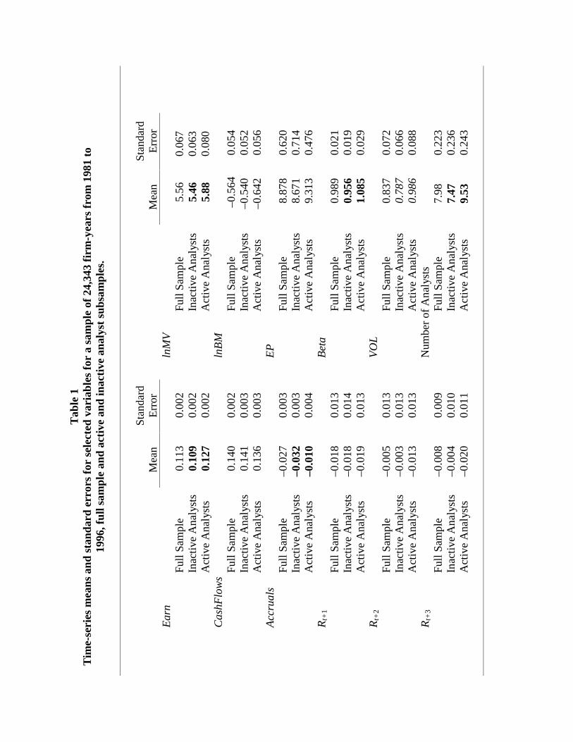
Tab

le 1

T

ime-

seri

es m

eans

and

sta

ndar

d er

rors

for

sel

ecte

d va

riab

les

for

a sa

mpl

e of

24,

343

firm

-yea

rs f

rom

198

1 to

19

96, f

ull s

ampl

e an

d ac

tive

and

inac

tive

ana

lyst

sub

sam

ples

.

Mea

n St

anda

rd

Err

or

Mea

n St

anda

rd

Err

or

Ear

n

lnM

V

F

ull S

ampl

e 0.

113

0.00

2

Ful

l Sam

ple

5.56

0.

067

Ina

ctiv

e A

naly

sts

0.10

9 0.

002

I

nact

ive

Ana

lyst

s 5.

46

0.06

3 A

ctiv

e A

naly

sts

0.12

7 0.

002

A

ctiv

e A

naly

sts

5.88

0.

080

Cas

hFlo

ws

lnB

M

F

ull S

ampl

e 0.

140

0.00

2

Ful

l Sam

ple

–0.5

64

0.05

4 I

nact

ive

Ana

lyst

s 0.

141

0.00

3

Ina

ctiv

e A

naly

sts

–0.5

40

0.05

2 A

ctiv

e A

naly

sts

0.13

6 0.

003

A

ctiv

e A

naly

sts

–0.6

42

0.05

6 A

ccru

als

E

P

F

ull S

ampl

e –0

.027

0.

003

F

ull S

ampl

e 8.

878

0.62

0 I

nact

ive

Ana

lyst

s –0

.032

0.

003

I

nact

ive

Ana

lyst

s 8.

671

0.71

4 A

ctiv

e A

naly

sts

–0.0

10

0.00

4

Act

ive

Ana

lyst

s 9.

313

0.47

6 R

t+1

B

eta

F

ull S

ampl

e –0

.018

0.

013

F

ull S

ampl

e 0.

989

0.02

1 I

nact

ive

Ana

lyst

s –0

.018

0.

014

I

nact

ive

Ana

lyst

s 0.

956

0.01

9 A

ctiv

e A

naly

sts

–0.0

19

0.01

3

Act

ive

Ana

lyst

s 1.

085

0.02

9 R

t+2

V

OL

Ful

l Sam

ple

–0.0

05

0.01

3

Ful

l Sam

ple

0.83

7 0.

072

Ina

ctiv

e A

naly

sts

–0.0

03

0.01

3

Ina

ctiv

e A

naly

sts

0.78

7 0.

066

Act

ive

Ana

lyst

s –0

.013

0.

013

A

ctiv

e A

naly

sts

0.98

6 0.

088

Rt+

3

Num

ber

of A

naly

sts

Ful

l Sam

ple

–0.0

08

0.00

9

Ful

l Sam

ple

7.98

0.

223

Ina

ctiv

e A

naly

sts

–0.0

04

0.01

0

Ina

ctiv

e A

naly

sts

7.47

0.

236

Act

ive

Ana

lyst

s –0

.020

0.

011

A

ctiv

e A

naly

sts

9.53

0.

243

41

Ear

n =

ear

ning

s fr

om c

ontin

uing

ope

ratio

ns a

fter

dep

reci

atio

n, s

cale

d by

ave

rage

tota

l ass

ets.

C

ashF

low

s =

Ear

n –

Acc

rual

s.

Acc

rual

s =

(∆C

A –

∆C

ASH

) –

(∆C

L –

∆ST

D)

– D

EP

, whe

re ∆

CA

= c

hang

e in

cur

rent

ass

ets,

∆C

ASH

= c

hang

e in

cas

h/ca

sh

equi

vale

nts,

∆C

L =

cha

nge

in c

urre

nt li

abil

itie

s, ∆

STD

= c

hang

e in

deb

t inc

lude

d in

cur

rent

liab

ilitie

s, a

nd D

EP

= d

epre

ciat

ion

and

amor

tiza

tion

exp

ense

, all

scal

ed b

y av

erag

e to

tal a

sset

s.

R =

Ann

ual s

ize-

adju

sted

ret

urns

fro

m th

e be

ginn

ing

of th

e fo

urth

mon

th a

fter

the

fisc

al y

ear

to th

e en

d of

the

fift

eent

h m

onth

aft

er th

e fi

scal

yea

r. R

etur

ns a

re th

e fi

rm’s

ret

urn

min

us th

e m

ean

retu

rn f

or th

e fi

rm’s

siz

e de

cile

, bas

ed o

n m

arke

t val

ue o

f eq

uity

at t

he

begi

nnin

g of

the

year

.

lnM

V =

nat

ural

loga

rith

m o

f th

e m

arke

t val

ue o

f eq

uity

.

lnB

M =

nat

ural

loga

rith

m o

f th

e bo

ok-t

o-m

arke

t rat

io.

E

P =

the

earn

ings

-to-

pric

e ra

tio.

B

eta

= b

eta

obta

ined

fro

m C

RSP

.

VO

L =

ann

ual t

radi

ng v

olum

e di

vide

d by

sha

res

outs

tand

ing.

N

umbe

r of

Ana

lyst

s fo

llow

ing

the

firm

is m

easu

red

in th

e m

onth

of

the

firm

’s f

isca

l yea

r en

d.

An

obse

rvat

ion

is in

clud

ed in

the

acti

ve a

naly

st s

ubsa

mpl

e if

the

mea

n co

nsen

sus

anal

yst f

orec

ast f

or y

ear

t + 1

is r

evis

ed a

t the

yea

r t

earn

ings

ann

ounc

emen

t in

the

dire

ctio

n im

plie

d by

a r

ever

sal o

f ye

ar t

accr

uals

; oth

erw

ise

it is

incl

uded

in th

e in

acti

ve a

naly

st

subs

ampl

e.

Bol

ded

(Ita

lici

zed)

am

ount

s in

dica

te th

at th

e tim

e-se

ries

mea

ns a

re d

iffe

rent

for

the

two

subs

ampl

es a

t a s

igni

fica

nce

leve

l of

0.05

(0

.10)

usi

ng a

two-

taile

d t-

test

.

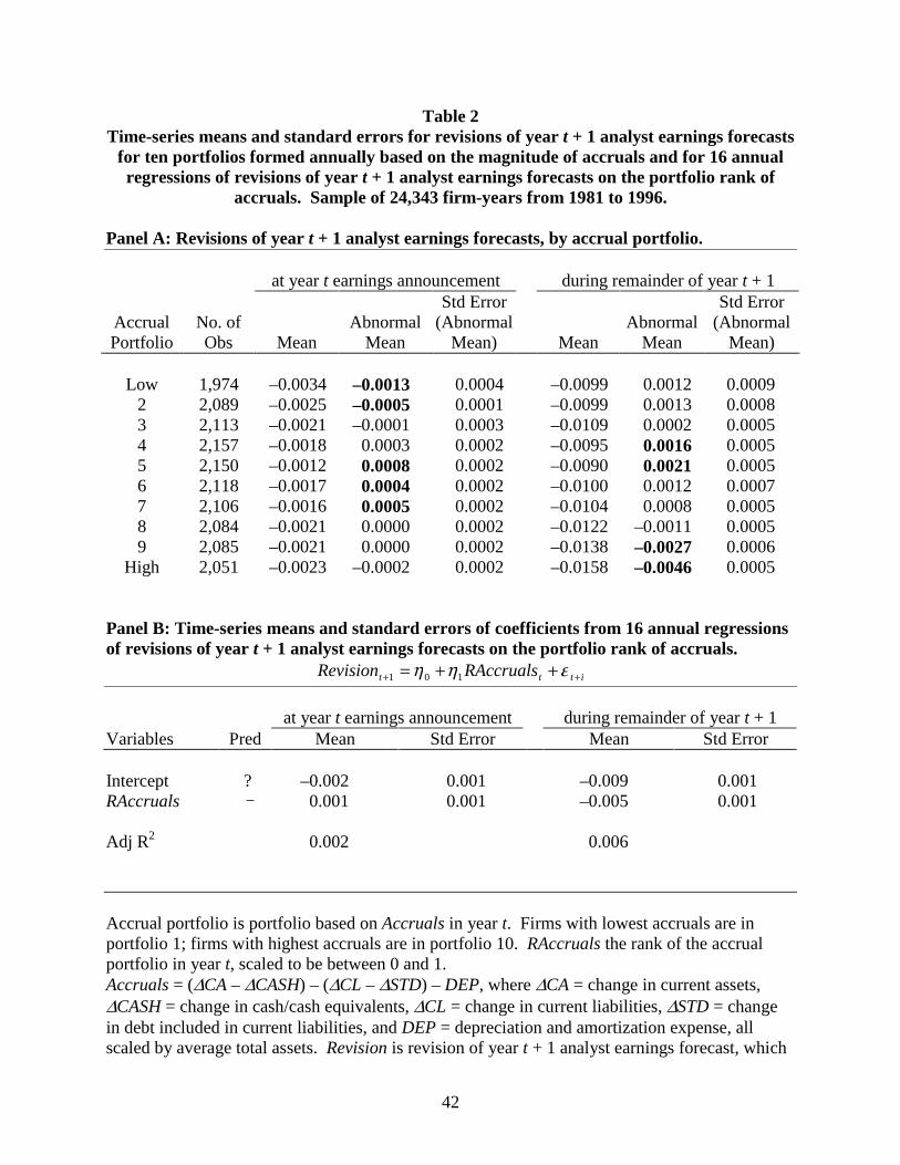
42

Table 2 Time-series means and standard errors for revisions of year t + 1 analyst earnings forecasts

for ten portfolios formed annually based on the magnitude of accruals and for 16 annual regressions of revisions of year t + 1 analyst earnings forecasts on the portfolio rank of

accruals. Sample of 24,343 firm-years from 1981 to 1996. Panel A: Revisions of year t + 1 analyst earnings forecasts, by accrual portfolio.

at year t earnings announcement during remainder of year t + 1

Accrual Portfolio

No. of Obs

Mean

Abnormal

Mean

Std Error (Abnormal

Mean)

Mean

Abnormal

Mean

Std Error (Abnormal

Mean)

Low 1,974 –0.0034 –0.0013 0.0004 –0.0099 0.0012 0.0009 2 2,089 –0.0025 –0.0005 0.0001 –0.0099 0.0013 0.0008 3 2,113 –0.0021 –0.0001 0.0003 –0.0109 0.0002 0.0005 4 2,157 –0.0018 0.0003 0.0002 –0.0095 0.0016 0.0005 5 2,150 –0.0012 0.0008 0.0002 –0.0090 0.0021 0.0005 6 2,118 –0.0017 0.0004 0.0002 –0.0100 0.0012 0.0007 7 2,106 –0.0016 0.0005 0.0002 –0.0104 0.0008 0.0005 8 2,084 –0.0021 0.0000 0.0002 –0.0122 –0.0011 0.0005 9 2,085 –0.0021 0.0000 0.0002 –0.0138 –0.0027 0.0006

High 2,051 –0.0023 –0.0002 0.0002 –0.0158 –0.0046 0.0005

Panel B: Time-series means and standard errors of coefficients from 16 annual regressions of revisions of year t + 1 analyst earnings forecasts on the portfolio rank of accruals.

ittt RAccrualsRevision ++ ++= εηη 101

at year t earnings announcement during remainder of year t + 1 Variables Pred Mean Std Error Mean Std Error

Intercept ? –0.002 0.001 –0.009 0.001 RAccruals – 0.001 0.001 –0.005 0.001

Adj R2 0.002 0.006

Accrual portfolio is portfolio based on Accruals in year t. Firms with lowest accruals are in portfolio 1; firms with highest accruals are in portfolio 10. RAccruals the rank of the accrual portfolio in year t, scaled to be between 0 and 1. Accruals = (∆CA – ∆CASH) – (∆CL – ∆STD) – DEP, where ∆CA = change in current assets, ∆CASH = change in cash/cash equivalents, ∆CL = change in current liabilities, ∆STD = change in debt included in current liabilities, and DEP = depreciation and amortization expense, all scaled by average total assets. Revision is revision of year t + 1 analyst earnings forecast, which

43

is measured as a change in the mean consensus forecast, with the earlier forecast subtracted from the later forecast, scaled by price at the end of year t. Abnormal forecast revision is the forecast revision in excess of the calendar-year mean revision for the same forecast period. Analyst forecast revision data are available for 20,927 observations. Bolded amounts indicate that the time-series means of abnormal forecast revisions are different for the two subsamples at a significance level of 0.05 using a two-tailed t-test.

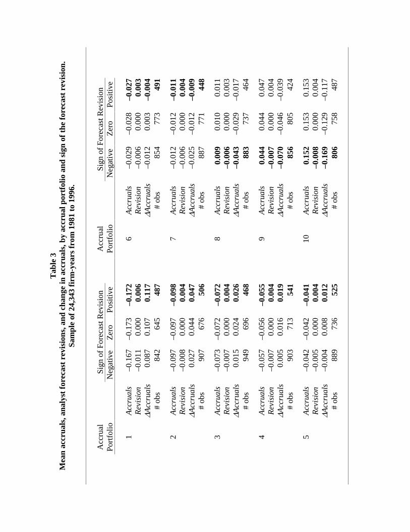
Tab

le 3

M

ean

accr

uals

, ana

lyst

for

ecas

t re

visi

ons,

and

cha

nge

in a

ccru

als,

by

accr

ual p

ortf

olio

and

sig

n of

the

for

ecas

t re

visi

on.

Sam

ple

of 2

4,34

3 fi

rm-y

ears

fro

m 1

981

to 1

996.

A

ccru

al

Si

gn o

f Fo

reca

st R

evis

ion

A

ccru

al

Si

gn o

f Fo

reca

st R

evis

ion

Port

folio

N

egat

ive

Zer

o Po

sitiv

e

Port

folio

N

egat

ive

Zer

o Po

sitiv

e

1 A

ccru

als

–0.1

67

–0.1

73

–0.1

72

6

Acc

rual

s –0

.029

–0

.028

–0

.027

Rev

isio

n –0

.011

0.

000

0.00

6

R

evis

ion

–0.0

06

0.00

0 0.

003

∆A

ccru

als

0.08

7 0.

107

0.11

7

∆A

ccru

als

–0.0

12

0.00

3 –0

.004

# ob

s 84

2 64

5 48

7

#

obs

854

773

491

2 A

ccru

als

–0.0

97

–0.0

97

–0.0

98

7

Acc

rual

s –0

.012

–0

.012

–0

.011

Rev

isio

n –0

.008

0.

000

0.00

4

R

evis

ion

–0.0

06

0.00

0 0.

004

∆A

ccru

als

0.02

7 0.

044

0.04

7

∆A

ccru

als

–0.0

25

–0.0

12

–0.0

09

#

obs

907

676

506

# ob

s 88

7 77

1 44

8

3 A

ccru

als

–0.0

73

–0.0

72

–0.0

72

8

Acc

rual

s 0.

009

0.01

0 0.

011

R

evis

ion

–0.0

07

0.00

0 0.

004

Rev

isio

n –0

.006

0.

000

0.00

3

∆Acc

rual

s 0.

015

0.02

4 0.

026

∆Acc

rual

s –0

.043

–0

.029

–0

.017

# ob

s 94

9 69

6 46

8

#

obs

883

737

464

4 A

ccru

als

–0.0

57

–0.0

56

–0.0

55

9

Acc

rual

s 0.

044

0.04

4 0.

047

R

evis

ion

–0.0

07

0.00

0 0.

004

Rev

isio

n –0

.007

0.

000

0.00

4

∆Acc

rual

s 0.

005

0.01

6 0.

019

∆Acc

rual

s –0

.070

–0

.046

–0

.039

# ob

s 90

3 71

3 54

1

#

obs

856

805

424

5 A

ccru

als

–0.0

42

–0.0

42

–0.0

41

10

A

ccru

als

0.15

2 0.

153

0.15

3

Rev

isio

n –0

.005

0.

000

0.00

4

R

evis

ion

–0.0

08

0.00

0 0.

004

∆A

ccru

als

–0.0

04

0.00

8 0.

012

∆Acc

rual

s –0

.169

–0

.129

–0

.117

# ob

s 88

9 73

6 52

5

#

obs

806

758

487

45

Acc

rual

Por

tfol

io is

the

accr

ual p

ortf

olio

in y

ear

t. L

owes

t acc

rual

s in

por

tfol

io 1

; Hig

hest

acc

rual

s in

por

tfol

io 1

0.

Acc

rual

s =

(∆C

A –

∆C

ASH

) –

(∆C

L –

∆ST

D)

– D

EP

, whe

re ∆

CA

= c

hang

e in

cur

rent

ass

ets,

∆C

ASH

= c

hang

e in

cas

h/ca

sh

equi

vale

nts,

∆C

L =

cha

nge

in c

urre

nt li

abil

itie

s, ∆

STD

= c

hang

e in

deb

t inc

lude

d in

cur

rent

liab

ilitie

s, a

nd D

EP

= d

epre

ciat

ion

and

amor

tiza

tion

exp

ense

, all

scal

ed b

y av

erag

e to

tal a

sset

s.

∆Acc

rual

s =

cha

nge

in a

ccru

als

is m

easu

red

as A

ccru

als

in y

ear

t + 1

min

us A

ccru

als

in y

ear

t, sc

aled

by

aver

age

tota

l ass

ets.

R

evis

ion

= a

naly

st f

orec

ast r

evis

ions

for

yea

r t +

1 e

arni

ngs

mad

e in

the

mon

th o

f ye

ar t

earn

ings

ann

ounc

emen

t. F

orec

ast r

evis

ions

ar

e m

easu

red

as c

hang

es in

the

mea

n co

nsen

sus

fore

cast

, wit

h th

e ea

rlie

r fo

reca

st s

ubtr

acte

d fr

om th

e la

ter

fore

cast

, sca

led

by p

rice

at

the

end

of y

ear

t. A

naly

st f

orec

ast r

evis

ion

data

are

ava

ilabl

e fo

r 20

,927

obs

erva

tions

.

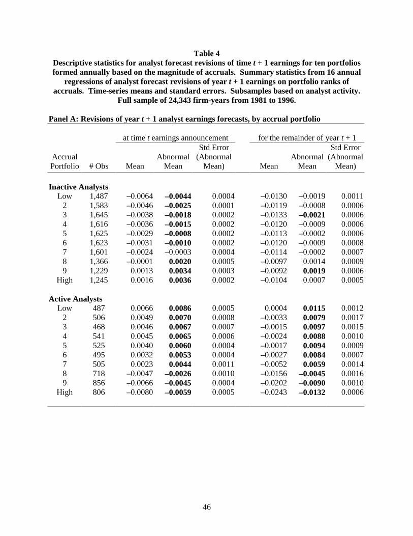
46

Table 4 Descriptive statistics for analyst forecast revisions of time t + 1 earnings for ten portfolios formed annually based on the magnitude of accruals. Summary statistics from 16 annual

regressions of analyst forecast revisions of year t + 1 earnings on portfolio ranks of accruals. Time-series means and standard errors. Subsamples based on analyst activity.

Full sample of 24,343 firm-years from 1981 to 1996. Panel A: Revisions of year t + 1 analyst earnings forecasts, by accrual portfolio

at time t earnings announcement for the remainder of year t + 1

Accrual Portfolio

# Obs

Mean

Abnormal

Mean

Std Error (Abnormal

Mean)

Mean

Abnormal

Mean

Std Error (Abnormal

Mean)

Inactive Analysts Low 1,487 –0.0064 –0.0044 0.0004 –0.0130 –0.0019 0.0011

2 1,583 –0.0046 –0.0025 0.0001 –0.0119 –0.0008 0.0006 3 1,645 –0.0038 –0.0018 0.0002 –0.0133 –0.0021 0.0006 4 1,616 –0.0036 –0.0015 0.0002 –0.0120 –0.0009 0.0006 5 1,625 –0.0029 –0.0008 0.0002 –0.0113 –0.0002 0.0006 6 1,623 –0.0031 –0.0010 0.0002 –0.0120 –0.0009 0.0008 7 1,601 –0.0024 –0.0003 0.0004 –0.0114 –0.0002 0.0007 8 1,366 –0.0001 0.0020 0.0005 –0.0097 0.0014 0.0009 9 1,229 0.0013 0.0034 0.0003 –0.0092 0.0019 0.0006

High 1,245 0.0016 0.0036 0.0002 –0.0104 0.0007 0.0005

Active Analysts Low 487 0.0066 0.0086 0.0005 0.0004 0.0115 0.0012

2 506 0.0049 0.0070 0.0008 –0.0033 0.0079 0.0017 3 468 0.0046 0.0067 0.0007 –0.0015 0.0097 0.0015 4 541 0.0045 0.0065 0.0006 –0.0024 0.0088 0.0010 5 525 0.0040 0.0060 0.0004 –0.0017 0.0094 0.0009 6 495 0.0032 0.0053 0.0004 –0.0027 0.0084 0.0007 7 505 0.0023 0.0044 0.0011 –0.0052 0.0059 0.0014 8 718 –0.0047 –0.0026 0.0010 –0.0156 –0.0045 0.0016 9 856 –0.0066 –0.0045 0.0004 –0.0202 –0.0090 0.0010

High 806 –0.0080 –0.0059 0.0005 –0.0243 –0.0132 0.0006

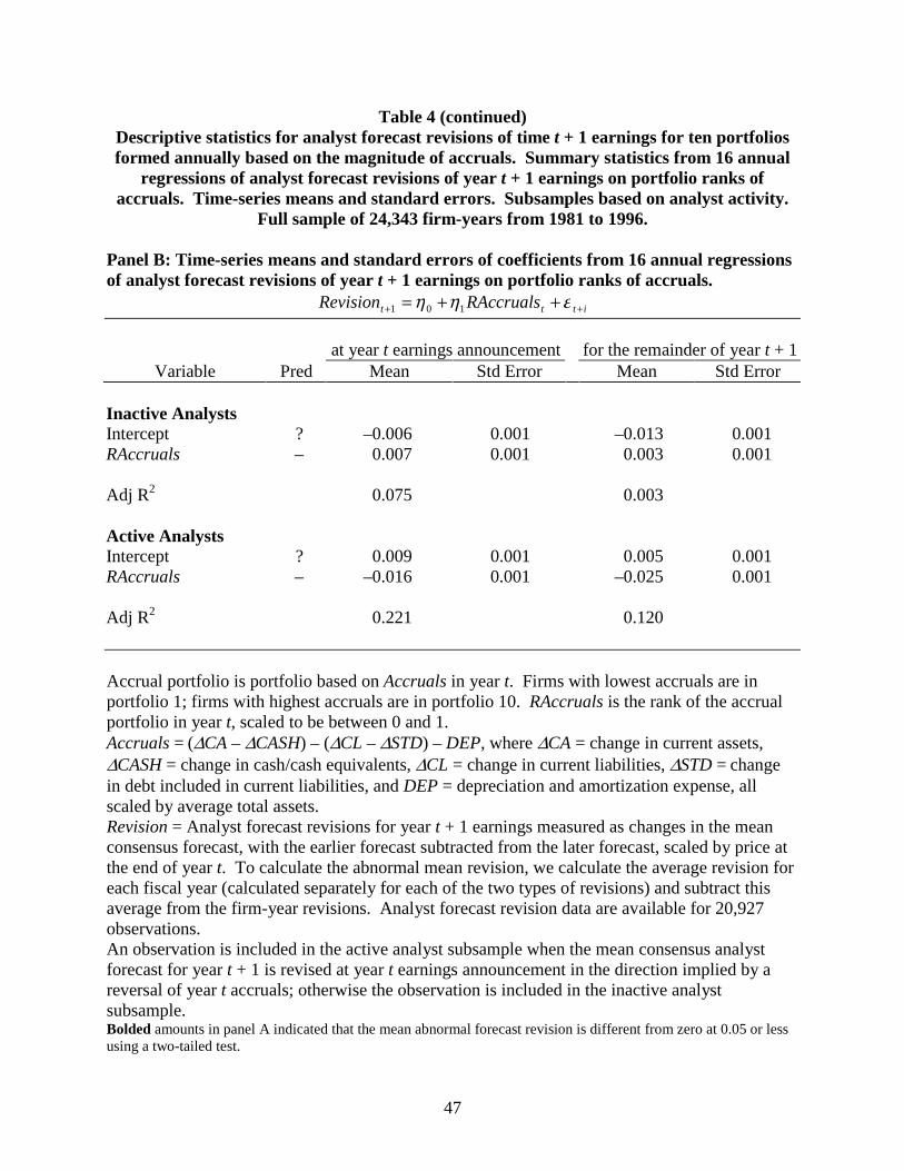
47

Table 4 (continued) Descriptive statistics for analyst forecast revisions of time t + 1 earnings for ten portfolios formed annually based on the magnitude of accruals. Summary statistics from 16 annual

regressions of analyst forecast revisions of year t + 1 earnings on portfolio ranks of accruals. Time-series means and standard errors. Subsamples based on analyst activity.

Full sample of 24,343 firm-years from 1981 to 1996. Panel B: Time-series means and standard errors of coefficients from 16 annual regressions of analyst forecast revisions of year t + 1 earnings on portfolio ranks of accruals.

ittt RAccrualsRevision ++ ++= εηη 101

at year t earnings announcement for the remainder of year t + 1

Variable Pred Mean Std Error Mean Std Error

Inactive Analysts Intercept ? –0.006 0.001 –0.013 0.001 RAccruals – 0.007 0.001 0.003 0.001

Adj R2 0.075 0.003 Active Analysts Intercept ? 0.009 0.001 0.005 0.001 RAccruals – –0.016 0.001 –0.025 0.001

Adj R2 0.221 0.120 Accrual portfolio is portfolio based on Accruals in year t. Firms with lowest accruals are in portfolio 1; firms with highest accruals are in portfolio 10. RAccruals is the rank of the accrual portfolio in year t, scaled to be between 0 and 1. Accruals = (∆CA – ∆CASH) – (∆CL – ∆STD) – DEP, where ∆CA = change in current assets, ∆CASH = change in cash/cash equivalents, ∆CL = change in current liabilities, ∆STD = change in debt included in current liabilities, and DEP = depreciation and amortization expense, all scaled by average total assets. Revision = Analyst forecast revisions for year t + 1 earnings measured as changes in the mean consensus forecast, with the earlier forecast subtracted from the later forecast, scaled by price at the end of year t. To calculate the abnormal mean revision, we calculate the average revision for each fiscal year (calculated separately for each of the two types of revisions) and subtract this average from the firm-year revisions. Analyst forecast revision data are available for 20,927 observations. An observation is included in the active analyst subsample when the mean consensus analyst forecast for year t + 1 is revised at year t earnings announcement in the direction implied by a reversal of year t accruals; otherwise the observation is included in the inactive analyst subsample. Bolded amounts in panel A indicated that the mean abnormal forecast revision is different from zero at 0.05 or less using a two-tailed test.

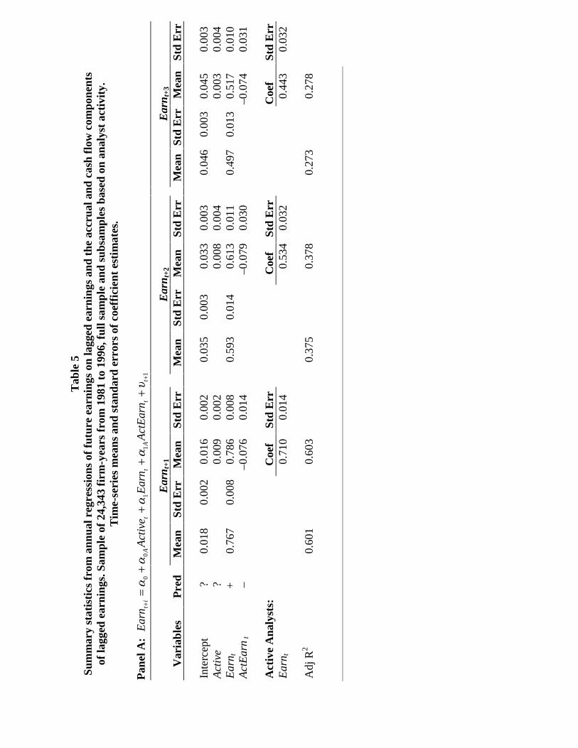
Tab

le 5

Su

mm

ary

stat

isti

cs f

rom

ann

ual r

egre

ssio

ns o

f fu

ture

ear

ning

s on

lagg

ed e

arni

ngs

and

the

accr

ual a

nd c

ash

flow

com

pone

nts

of la

gged

ear

ning

s. S

ampl

e of

24,

343

firm

-yea

rs f

rom

198

1 to

199

6, f

ull s

ampl

e an

d su

bsam

ples

bas

ed o

n an

alys

t ac

tivi

ty.

Tim

e-se

ries

mea

ns a

nd s

tand

ard

erro

rs o

f co

effi

cien

t es

tim

ates

. P

anel

A:

11

10

0+

++

++

+=

tt

At

tA

it

Act

Ear

nE

arn

Act

ive

Ear

nυ

αα

αα

E

arn t

+1

E

arn t

+2

E

arn t

+3

Var

iabl

es

Pre

d M

ean

St

d E

rr

Mea

n St

d E

rr

M

ean

St

d E

rr

Mea

n

Std

Err

Mea

n S

td E

rr

Mea

n

Std

Err

In

terc

ept

?

0.01

8 0.

002

0.01

6 0.

002

0.

035

0.00

3 0.

033

0.00

3

0.04

6 0.

003

0.04

5 0.

003

Act

ive

?

0.00

9 0.

002

0.

008

0.00

4

0.00

3 0.

004

Ear

n t

+

0.

767

0.00

8 0.

786

0.00

8

0.59

3 0.

014

0.61

3 0.

011

0.

497

0.01

3 0.

517

0.01

0 A

ctE

arn

t –

–0

.076

0.

014

–0

.079

0.

030

–0.

074

0.03

1

Act

ive

Ana

lyst

s:

C

oef

Std

Err

Coe

f St

d E

rr

Coe

f St

d E

rr

Ear

n t

0.

710

0.01

4

0.53

4 0.

032

0.

443

0.03

2

A

dj R

2

0.60

1

0.60

3

0.

375

0.

378

0.27

3

0.27

8

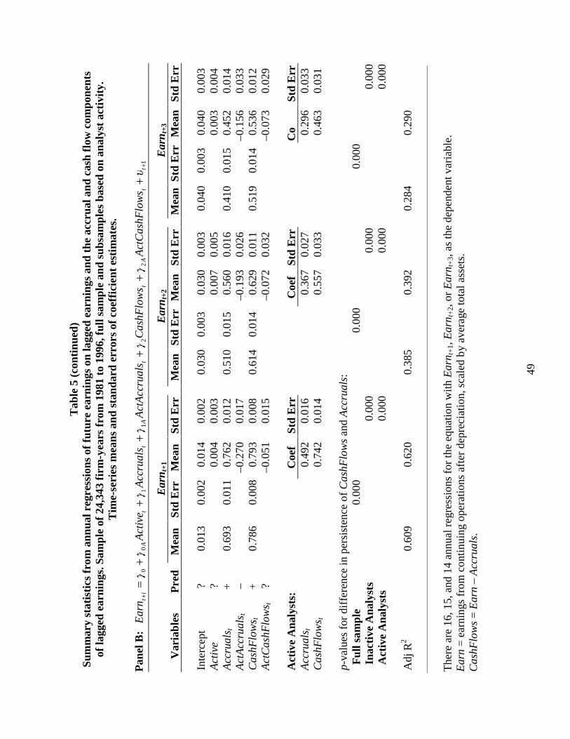
49

Tab

le 5

(co

ntin

ued)

Su

mm

ary

stat

isti

cs f

rom

ann

ual r

egre

ssio

ns o

f fu

ture

ear

ning

s on

lagg

ed e

arni

ngs

and

the

accr

ual a

nd c

ash

flow

com

pone

nts

of la

gged

ear

ning

s. S

ampl

e of

24,

343

firm

-yea

rs f

rom

198

1 to

199

6, f

ull s

ampl

e an

d su

bsam

ples

bas

ed o

n an

alys

t ac

tivi

ty.

Tim

e-se

ries

mea

ns a

nd s

tand

ard

erro

rs o

f co

effi

cien

t es

tim

ates

. P

anel

B:

1

22

11

00

++

++

++

++

=t

tA

tt

At

tA

it

ws

Act

Cas

hFlo

Cas

hFlo

ws

sA

ctA

ccru

alA

ccru

als

Act

ive

Ear

nυ

γγ

γγ

γγ

E

arn t

+1

E

arn t

+2

E

arn t

+3

Var

iabl

es

Pre

d M

ean

St

d E

rr

Mea

n St

d E

rr

M

ean

Std

Err

M

ean

Std

Err

Mea

n St

d E

rr

Mea

n S

td E

rr

Inte

rcep

t ?

0.01

3 0.

002

0.01

4 0.

002

0.

030

0.00

3 0.

030

0.00

3

0.04

0 0.

003

0.04

0 0.

003

Act

ive

?

0.

004

0.00

3

0.00

7 0.

005

0.

003

0.00

4 A

ccru

als t

+

0.

693

0.01

1 0.

762

0.01

2

0.51

0 0.

015

0.56

0 0.

016

0.

410

0.01

5 0.

452

0.01

4 A

ctA

ccru

als t

–

–0.2

70

0.01

7

–0.1

93

0.02

6

–

0.15

6 0.

033

Cas

hFlo

ws t

+

0.

786

0.00

8 0.

793

0.00

8

0.61

4 0.

014

0.62

9 0.

011

0.

519

0.01

4 0.

536

0.01

2 A

ctC

ashF

low

s t

?

–0

.051

0.

015

–0

.072

0.

032

–0

.073

0.

029

A

ctiv

e A

naly

sts:

Coe

f St

d E

rr

C

oef

Std

Err

C

o St

d E

rr

Acc

rual

s t

0.49

2 0.

016

0.

367

0.02

7

0.29

6 0.

033

Cas

hFlo

ws t

0.

742

0.01

4

0.55

7 0.

033

0.

463

0.03

1

p-va

lues

for

dif

fere

nce

in p

ersi

sten

ce o

f C

ashF

low

s an

d A

ccru

als:

F

ull s

ampl

e

0.00

0

0.

000

0.00

0

I

nact

ive

Ana

lyst

s

0.

000

0.00

0

0.

000

Act

ive

Ana

lyst

s

0.

000

0.00

0

0.

000

A

dj R

2 0.

609

0.

620

0.38

5

0.39

2

0.

284

0.

290

The

re a

re 1

6, 1

5, a

nd 1

4 an

nual

reg

ress

ions

for

the

equa

tion

with

Ear

n t+

1, E

arn t

+2, o

r E

arn t

+3, a

s th

e de

pend

ent v

aria

ble.

E

arn

= e

arni

ngs

from

con

tinui

ng o

pera

tions

aft

er d

epre

ciat

ion,

sca

led

by a

vera

ge to

tal a

sset

s.

Cas

hFlo

ws

= E

arn

– A

ccru

als.

50

Acc

rual

s =

(∆C

A –

∆C

ASH

) –

(∆C

L –

∆ST

D)

– D

EP

, whe

re ∆

CA

= c

hang

e in

cur

rent

ass

ets,

∆C

ASH

= c

hang

e in

cas

h/ca

sh

equi

vale

nts,

∆C

L =

cha

nge

in c

urre

nt li

abil

itie

s, ∆

STD

= c

hang

e in

deb

t inc

lude

d in

cur

rent

liab

ilitie

s, a

nd D

EP

= d

epre

ciat

ion

and

amor

tiza

tion

exp

ense

, all

scal

ed b

y av

erag

e to

tal a

sset

s.

Act

ive

is a

n in

dica

tor

vari

able

whi

ch e

qual

s 1

whe

n th

e m

ean

cons

ensu

s an

alys

t for

ecas

t for

yea

r t +

1 is

rev

ised

at y

ear

t ear

ning

s an

noun

cem

ent i

n th

e di

rect

ion

impl

ied

by a

rev

ersa

l of

year

t ac

crua

ls, a

nd 0

oth

erw

ise.

A

ctE

arn

= A

ctiv

e ×

Ear

n; A

ctA

ccru

als

= A

ctiv

e ×

Acc

rual

s; A

ctC

ashF

low

s =

Act

ive

× C

ashF

low

s.

p-va

lues

in p

anel

B a

re a

ssoc

iate

d w

ith

F-te

sts

of w

heth

er th

e pe

rsis

tenc

e of

acc

rual

s an

d ca

sh f

low

s si

gnif

ican

tly

diff

er.

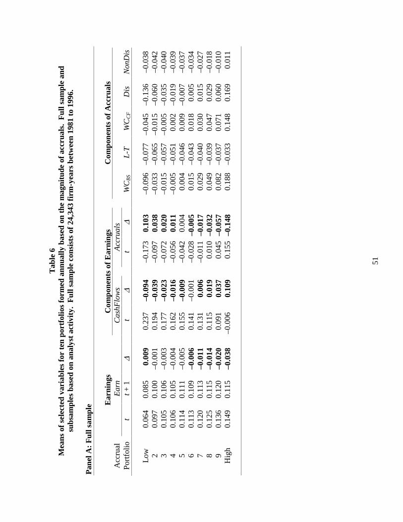
51

Tab

le 6

M

eans

of

sele

cted

var

iabl

es f

or t

en p

ortf

olio

s fo

rmed

ann

ually

bas

ed o

n th

e m

agni

tude

of

accr

uals

. F

ull s

ampl

e an

d su

bsam

ples

bas

ed o

n an

alys

t ac

tivi

ty.

Ful

l sam

ple

cons

ists

of

24,3

43 f

irm

-yea

rs b

etw

een

1981

to

1996

. P

anel

A:

Ful

l sam

ple

Ear

ning

s

Com

pone

nts

of E

arni

ngs

C

ompo

nent

s of

Acc

rual

s A

ccru

al

E

arn

Cas

hFlo

ws

A

ccru

als

Por

tfol

io

t t +

1

∆

t ∆

t

∆

WC

BS

L-T

W

CC

F

Dis

N

onD

is

Low

0.

064

0.08

5 0.

009

0.

237

–0.0

94

–0

.173

0.

103

–0

.096

–0

.077

–0

.045

–0

.136

–0

.038

2

0.09

7 0.

100

–0.0

01

0.

194

–0.0

39

–0

.097

0.

038

–0

.033

–0

.065

–0

.015

–0

.060

–0

.042

3

0.10

5 0.

106

–0.0

03

0.

177

–0.0

23

–0

.072

0.

020

–0

.015

–0

.057

–0

.005

–0

.035

–0

.040

4

0.10

6 0.

105

–0.0

04

0.

162

–0.0

16

–0

.056

0.

011

–0

.005

–0

.051

0.

002

–0.0

19

–0.0

39

5 0.

114

0.11

1 –0

.005

0.15

5 –0

.009

–0.0

42

0.00

4

0.00

4 –0

.046

0.

009

–0.0

07

–0.0

37

6 0.

113

0.10

9 –0

.006

0.14

1 –0

.001

–0.0

28

–0.0

05

0.

015

–0.0

43

0.01

8 0.

005

–0.0

34

7 0.

120

0.11

3 –0

.011

0.13

1 0.

006

–0

.011

–0

.017

0.02

9 –0

.040

0.

030

0.01

5 –0

.027

8

0.12

5 0.

115

–0.0

14

0.

115

0.01

9

0.01

0 –0

.032

0.04

9 –0

.039

0.

047

0.02

9 –0

.018

9

0.13

6 0.

120

–0.0

20

0.

091

0.03

7

0.04

5 –0

.057

0.08

2 –0

.037

0.

071

0.06

0 –0

.010

H

igh

0.14

9 0.

115

–0.0

38

–0

.006

0.

109

0.

155

–0.1

48

0.

188

–0.0

33

0.14

8 0.

169

0.01

1

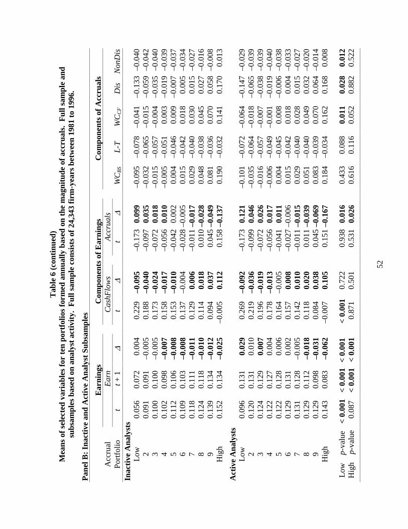
52

Tab

le 6

(co

ntin

ued)

M

eans

of

sele

cted

var

iabl

es f

or t

en p

ortf

olio

s fo

rmed

ann

ually

bas

ed o

n th

e m

agni

tude

of

accr

uals

. F

ull s

ampl

e an

d su

bsam

ples

bas

ed o

n an

alys

t ac

tivi

ty.

Ful

l sam

ple

cons

ists

of

24,3

43 f

irm

-yea

rs b

etw

een

1981

to

1996

. P

anel

B:

Inac

tive

and

Act

ive

Ana

lyst

Sub

sam

ples

E

arni

ngs

C

ompo

nent

s of

Ear

ning

s

Com

pone

nts

of A

ccru

als

Acc

rual

Ear

n

C

ashF

low

s

Acc

rual

s

P

ortf

olio

t

t + 1

∆

t

∆

t ∆

W

CB

S L

-T

WC

CF

Dis

N

onD

is

Inac

tive

Ana

lyst

s

L

ow

0.05

6 0.

072

0.00

4

0.22

9 –0

.095

–0.1

73

0.09

9

–0.0

95

–0.0

78

–0.0

41

–0.1

33

–0.0

40

2 0.

091

0.09

1 –0

.005

0.18

8 –0

.040

–0.0

97

0.03

5

–0.0

32

–0.0

65

–0.0

15

–0.0

59

–0.0

42

3 0.

100

0.10

0 –0

.005

0.17

3 –0

.024

–0.0

72

0.01

8

–0.0

15

–0.0

57

–0.0

04

–0.0

35

–0.0

40

4 0.

102

0.09

8 –0

.007

0.15

8 –0

.017

–0.0

56

0.01

0

–0.0

05

–0.0

51

0.00

3 –0

.019

–0

.039

5

0.11

2 0.

106

–0.0

08

0.

153

–0.0

10

–0

.042

0.

002

0.

004

–0.0

46

0.00

9 –0

.007

–0

.037

6

0.10

9 0.

103

–0.0

08

0.

137

–0.0

04

–0

.028

–0.

005

0.

015

–0.0

42

0.01

8 0.

005

–0.0

34

7 0.

118

0.11

1 –0

.011

0.12

9 0.

006

–0

.011

–0.

017

0.

029

–0.0

40

0.03

0 0.

015

–0.0

27

8 0.

124

0.11

8 –0

.010

0.11

4 0.

018

0.

010

–0.0

28

0.

048

–0.0

38

0.04

5 0.

027

–0.0

16

9 0.

139

0.13

4 –0

.012

0.09

4 0.

037

0.

045

–0.0

49

0.

081

–0.0

36

0.07

0 0.

058

–0.0

08

Hig

h 0.

152

0.13

4 –0

.025

–0.0

05

0.11

2

0.15

8 –0

.137

0.19

0 –0

.032

0.

141

0.17

0 0.

013

Act

ive

Ana

lyst

s

L

ow

0.09

6 0.

131

0.02

9

0.26

9 –0

.092

–0.1

73

0.12

1

–0.1

01

–0.0

72

–0.0

64

–0.1

47

–0.0

29

2 0.

120

0.13

1 0.

010

0.

219

–0.0

36

–0

.099

0.

046

–0

.035

–0

.064

–0

.018

–0

.065

–0

.039

3

0.12

4 0.

129

0.00

7

0.19

6 –0

.019

–0.0

72

0.02

6

–0.0

16

–0.0

57

–0.0

07

–0.0

38

–0.0

39

4 0.

122

0.12

7 0.

004

0.

178

–0.0

13

–0

.056

0.

017

–0

.006

–0

.049

–0

.001

–0

.019

–0

.040

5

0.12

2 0.

128

0.00

6

0.16

4 –0

.005

–0.0

41

0.01

1

0.00

4 –0

.045

0.

008

–0.0

06

–0.0

38

6 0.

129

0.13

1 0.

002

0.

157

0.00

8

–0.0

27 –

0.00

6

0.01

5 –0

.042

0.

018

0.00

4 –0

.033

7

0.13

1 0.

128

–0.0

05

0.

142

0.01

0

–0.0

11 –

0.01

5

0.02

9 –0

.040

0.

028

0.01

5 –0

.027

8

0.12

9 0.

112

–0.0

18

0.

118

0.02

0

0.01

1 –0

.039

0.05

1 –0

.040

0.

049

0.03

2 –0

.020

9

0.12

9 0.

098

–0.0

31

0.

084

0.03

8

0.04

5 –0

.069

0.08

3 –0

.039

0.

070

0.06

4 –0

.014

H

igh

0.14

3 0.

083

–0.0

62

–0

.007

0.

105

0.

151

–0.1

67

0.

184

–0.0

34

0.16

2 0.

168

0.00

8

L

ow

p-v

alue

<

0.0

01

< 0.

001

< 0.

001

<

0.00

1 0.

722

0.

938

0.01

6

0.43

3 0.

088

0.01

1 0.

028

0.01

2 H

igh

p-

valu

e 0.

087

< 0.

001

< 0.

001

0.

871

0.50

1

0.53

1 0.

026

0.

616

0.11

6 0.

052

0.88

2 0.

522

53

Ear

n =

ear

ning

s fr

om c

ontin

uing

ope

ratio

ns a

fter

dep

reci

atio

n, s

cale

d by

ave

rage

tota

l ass

ets.

C

ashF

low

s =

Ear

n –

Acc

rual

s.

Acc

rual

s =

(∆C

A –

∆C

ASH

) –

(∆C

L –

∆ST

D)

– D

EP

, whe

re ∆

CA

= c

hang

e in

cur

rent

ass

ets,

∆C

ASH

= c

hang

e in

cas

h/ca

sh

equi

vale

nts,

∆C

L =

cha

nge

in c

urre

nt li

abil

itie

s, ∆

STD

= c

hang

e in

deb

t inc

lude

d in

cur

rent

liab

ilitie

s, a

nd D

EP

= d

epre

ciat

ion

and

amor

tiza

tion

exp

ense

, all

scal

ed b

y av

erag

e to

tal a

sset

s.

Acc

rual

Por

tfol

io is

the

accr

ual p

ortf

olio

in y

ear

t. L

owes

t acc

rual

s in

por

tfol

io 1

; Hig

hest

acc

rual

s in

por

tfol

io 1

0.

∆ de

note

s ch

ange

fro

m y

ear

t to

year

t +

1.

WC

BS

= w

orki

ng c

apita

l acc

rual

s, c

alcu

late

d us

ing

chan

ges

in w

orki

ng c

apita

l acc

ount

s fr

om th

e ba

lanc

e sh

eet (

# 1,

4, 5

, 34)

, sca

led

by

aver

age

tota

l ass

ets.

L

-T =

Acc

rual

s –

WC

BS.

W

CC

F =

wor

king

cap

ital a

ccru

als,

cal

cula

ted

usin

g ch

ange

s in

wor

king

cap

ital a

ccou

nts

from

the

stat

emen

t of

cash

flo

ws

(# 3

02, 3

03,

304,

305

and

307

), s

cale

d by

ave

rage

tota

l ass

ets.

D

is =

dis

cret

iona

ry a

ccru

als,

cal

cula

ted

as th

e re

sidu

als

from

ann

ual c

ross

-sec

tiona

l est

imat

ions

of

the

mod

ifie

d Jo

nes

mod

el (

see

Dec

how

, Slo

an a

nd S

wee

ney

[199

6]).

N

onD

is =

Acc

rual

s –

Dis

. A

n ob

serv

atio

n is

incl

uded

in th

e ac

tive

ana

lyst

sub

sam

ple

whe

n th

e m

ean

cons

ensu

s an

alys

t for

ecas

t for

yea

r t +

1 is

rev

ised

at y

ear

t ea

rnin

gs a

nnou

ncem

ent i

n th

e di

rect

ion

impl

ied

by a

rev

ersa

l of

year

t ac

crua

ls; o

ther

wis

e th

e ob

serv

atio

n is

incl

uded

in th

e in

acti

ve

anal

yst s

ubsa

mpl

e.

Bol

ded

amou

nts

indi

cate

that

the

mea

n ∆E

arn

is s

igni

fica

ntly

dif

fere

nt f

rom

zer

o at

0.0

5 or

less

usi

ng a

two-

taile

d te

st.

p-va

lues

indi

cate

the

sign

ific

ance

of

the

diff

eren

ce in

mea

ns b

etw

een

the

acti

ve a

nd in

acti

ve s

ampl

e fo

r th

e L

ow a

nd H

igh

accr

ual

port

folio

s. p

-val

ues

less

than

0.0

5 ar

e bo

lded

.

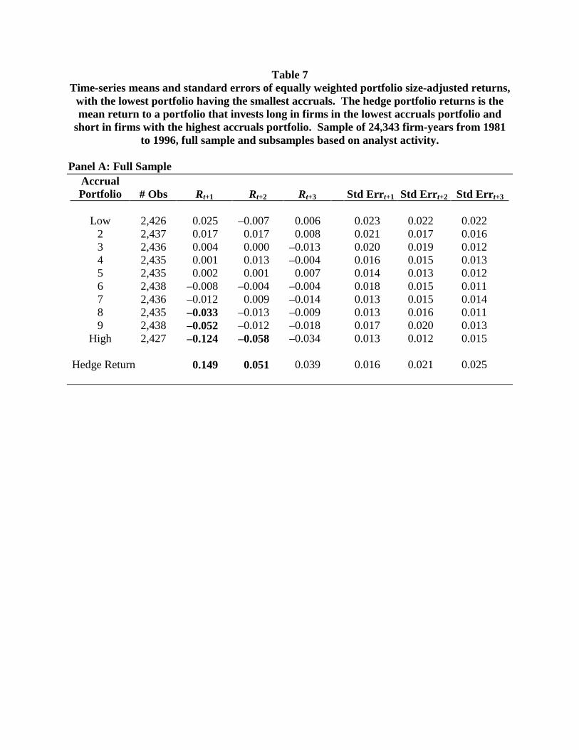
Table 7 Time-series means and standard errors of equally weighted portfolio size-adjusted returns,

with the lowest portfolio having the smallest accruals. The hedge portfolio returns is the mean return to a portfolio that invests long in firms in the lowest accruals portfolio and

short in firms with the highest accruals portfolio. Sample of 24,343 firm-years from 1981 to 1996, full sample and subsamples based on analyst activity.

Panel A: Full Sample

Accrual Portfolio # Obs Rt+1 Rt+2 Rt+3 Std Errt+1 Std Errt+2 Std Errt+3

Low 2,426 0.025 –0.007 0.006 0.023 0.022 0.022

2 2,437 0.017 0.017 0.008 0.021 0.017 0.016 3 2,436 0.004 0.000 –0.013 0.020 0.019 0.012 4 2,435 0.001 0.013 –0.004 0.016 0.015 0.013 5 2,435 0.002 0.001 0.007 0.014 0.013 0.012 6 2,438 –0.008 –0.004 –0.004 0.018 0.015 0.011 7 2,436 –0.012 0.009 –0.014 0.013 0.015 0.014 8 2,435 –0.033 –0.013 –0.009 0.013 0.016 0.011 9 2,438 –0.052 –0.012 –0.018 0.017 0.020 0.013

High 2,427 –0.124 –0.058 –0.034 0.013 0.012 0.015

Hedge Return 0.149 0.051 0.039 0.016 0.021 0.025

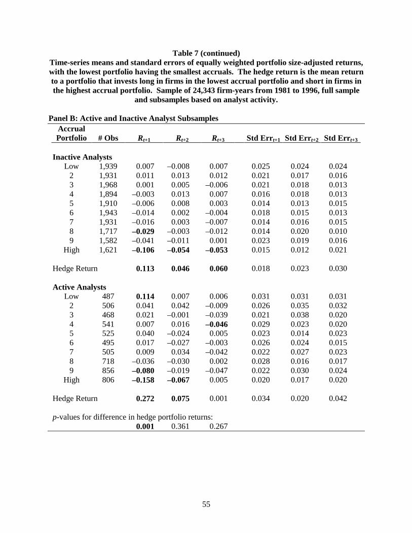
55

Table 7 (continued) Time-series means and standard errors of equally weighted portfolio size-adjusted returns, with the lowest portfolio having the smallest accruals. The hedge return is the mean return to a portfolio that invests long in firms in the lowest accrual portfolio and short in firms in the highest accrual portfolio. Sample of 24,343 firm-years from 1981 to 1996, full sample

and subsamples based on analyst activity.

Panel B: Active and Inactive Analyst Subsamples Accrual Portfolio # Obs Rt+1 Rt+2 Rt+3 Std Errt+1 Std Errt+2 Std Errt+3

Inactive Analysts

Low 1,939 0.007 –0.008 0.007 0.025 0.024 0.024 2 1,931 0.011 0.013 0.012 0.021 0.017 0.016 3 1,968 0.001 0.005 –0.006 0.021 0.018 0.013 4 1,894 –0.003 0.013 0.007 0.016 0.018 0.013 5 1,910 –0.006 0.008 0.003 0.014 0.013 0.015 6 1,943 –0.014 0.002 –0.004 0.018 0.015 0.013 7 1,931 –0.016 0.003 –0.007 0.014 0.016 0.015 8 1,717 –0.029 –0.003 –0.012 0.014 0.020 0.010 9 1,582 –0.041 –0.011 0.001 0.023 0.019 0.016

High 1,621 –0.106 –0.054 –0.053 0.015 0.012 0.021

Hedge Return 0.113 0.046 0.060 0.018 0.023 0.030

Active Analysts Low 487 0.114 0.007 0.006 0.031 0.031 0.031

2 506 0.041 0.042 –0.009 0.026 0.035 0.032 3 468 0.021 –0.001 –0.039 0.021 0.038 0.020 4 541 0.007 0.016 –0.046 0.029 0.023 0.020 5 525 0.040 –0.024 0.005 0.023 0.014 0.023 6 495 0.017 –0.027 –0.003 0.026 0.024 0.015 7 505 0.009 0.034 –0.042 0.022 0.027 0.023 8 718 –0.036 –0.030 0.002 0.028 0.016 0.017 9 856 –0.080 –0.019 –0.047 0.022 0.030 0.024

High 806 –0.158 –0.067 0.005 0.020 0.017 0.020

Hedge Return 0.272 0.075 0.001 0.034 0.020 0.042

p-values for difference in hedge portfolio returns: 0.001 0.361 0.267

56

Portfolios are formed annually by assigning firms into deciles based on the magnitude of accruals in year t. The reported means and standard errors are based on the time-series of the annual portfolio size-adjusted stock returns. R = Annual size-adjusted returns from the beginning of the fourth month after the fiscal year to the end of the fifteenth month after the fiscal year. Returns are the firm’s return minus the mean return for the firm’s size decile, based on market value of equity at the beginning of the year. Accrual Portfolio is the accrual portfolio in year t. Lowest accruals in portfolio 1; Highest accruals in portfolio 10, where Accruals = (∆CA – ∆CASH) – (∆CL – ∆STD) – DEP, where ∆CA = change in current assets, ∆CASH = change in cash/cash equivalents, ∆CL = change in current liabilities, ∆STD = change in debt included in current liabilities, and DEP = depreciation and amortization expense, all scaled by average total assets. An observation is in the active analyst subsample when the mean consensus analyst forecast for year t + 1 is revised at the year t earnings announcement in the direction implied by a reversal of year t accruals; otherwise the observation is in the inactive analyst subsample.

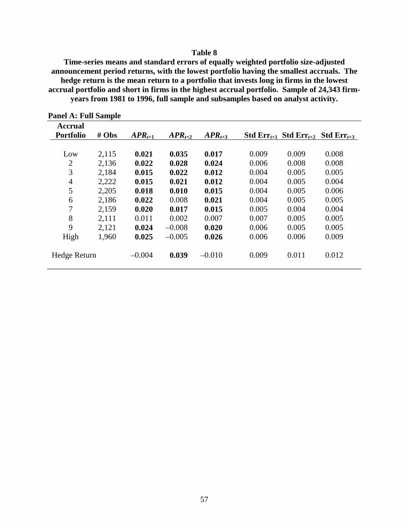
57

Table 8 Time-series means and standard errors of equally weighted portfolio size-adjusted

announcement period returns, with the lowest portfolio having the smallest accruals. The hedge return is the mean return to a portfolio that invests long in firms in the lowest

accrual portfolio and short in firms in the highest accrual portfolio. Sample of 24,343 firm-years from 1981 to 1996, full sample and subsamples based on analyst activity.

Panel A: Full Sample

Accrual Portfolio # Obs APRt+1 APRt+2 APRt+3 Std Errt+1 Std Errt+2 Std Errt+3

Low 2,115 0.021 0.035 0.017 0.009 0.009 0.008

2 2,136 0.022 0.028 0.024 0.006 0.008 0.008 3 2,184 0.015 0.022 0.012 0.004 0.005 0.005 4 2,222 0.015 0.021 0.012 0.004 0.005 0.004 5 2,205 0.018 0.010 0.015 0.004 0.005 0.006 6 2,186 0.022 0.008 0.021 0.004 0.005 0.005 7 2,159 0.020 0.017 0.015 0.005 0.004 0.004 8 2,111 0.011 0.002 0.007 0.007 0.005 0.005 9 2,121 0.024 –0.008 0.020 0.006 0.005 0.005

High 1,960 0.025 –0.005 0.026 0.006 0.006 0.009

Hedge Return –0.004 0.039 –0.010 0.009 0.011 0.012

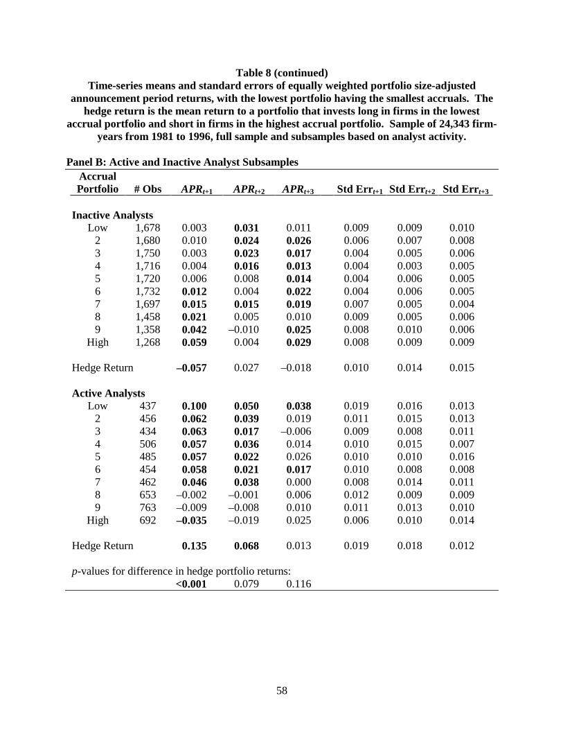
58

Table 8 (continued) Time-series means and standard errors of equally weighted portfolio size-adjusted

announcement period returns, with the lowest portfolio having the smallest accruals. The hedge return is the mean return to a portfolio that invests long in firms in the lowest

accrual portfolio and short in firms in the highest accrual portfolio. Sample of 24,343 firm-years from 1981 to 1996, full sample and subsamples based on analyst activity.

Panel B: Active and Inactive Analyst Subsamples

Accrual Portfolio # Obs APRt+1 APRt+2 APRt+3 Std Errt+1 Std Errt+2 Std Errt+3

Inactive Analysts

Low 1,678 0.003 0.031 0.011 0.009 0.009 0.010 2 1,680 0.010 0.024 0.026 0.006 0.007 0.008 3 1,750 0.003 0.023 0.017 0.004 0.005 0.006 4 1,716 0.004 0.016 0.013 0.004 0.003 0.005 5 1,720 0.006 0.008 0.014 0.004 0.006 0.005 6 1,732 0.012 0.004 0.022 0.004 0.006 0.005 7 1,697 0.015 0.015 0.019 0.007 0.005 0.004 8 1,458 0.021 0.005 0.010 0.009 0.005 0.006 9 1,358 0.042 –0.010 0.025 0.008 0.010 0.006

High 1,268 0.059 0.004 0.029 0.008 0.009 0.009

Hedge Return –0.057 0.027 –0.018 0.010 0.014 0.015

Active Analysts Low 437 0.100 0.050 0.038 0.019 0.016 0.013

2 456 0.062 0.039 0.019 0.011 0.015 0.013 3 434 0.063 0.017 –0.006 0.009 0.008 0.011 4 506 0.057 0.036 0.014 0.010 0.015 0.007 5 485 0.057 0.022 0.026 0.010 0.010 0.016 6 454 0.058 0.021 0.017 0.010 0.008 0.008 7 462 0.046 0.038 0.000 0.008 0.014 0.011 8 653 –0.002 –0.001 0.006 0.012 0.009 0.009 9 763 –0.009 –0.008 0.010 0.011 0.013 0.010

High 692 –0.035 –0.019 0.025 0.006 0.010 0.014

Hedge Return 0.135 0.068 0.013 0.019 0.018 0.012

p-values for difference in hedge portfolio returns: <0.001 0.079 0.116

59

Portfolios are formed annually by assigning firms into deciles based on the magnitude of accruals in year t. The reported means and standard errors are based on the time-series of the annual portfolio size-adjusted stock returns. APRt = Announcement period returns, the cumulative returns over the four fourteen-day periods (–11 to +2) around each of the earnings announcements in the fiscal years following the portfolio formation year, year t. Announcement period returns are available for 21,399 observations. Accrual Portfolio is the accrual portfolio in year t. Lowest accruals in portfolio 1; highest accruals in portfolio 10, where Accruals = (∆CA – ∆CASH) – (∆CL – ∆STD) – DEP, where ∆CA = change in current assets, ∆CASH = change in cash/cash equivalents, ∆CL = change in current liabilities, ∆STD = change in debt included in current liabilities, and DEP = depreciation and amortization expense, all scaled by average total assets. An observation is in the active analyst subsample when the mean consensus analyst forecast for year t + 1 is revised at the year t earnings announcement in the direction implied by a reversal of year t accruals; otherwise the observation is in the inactive analyst subsample.

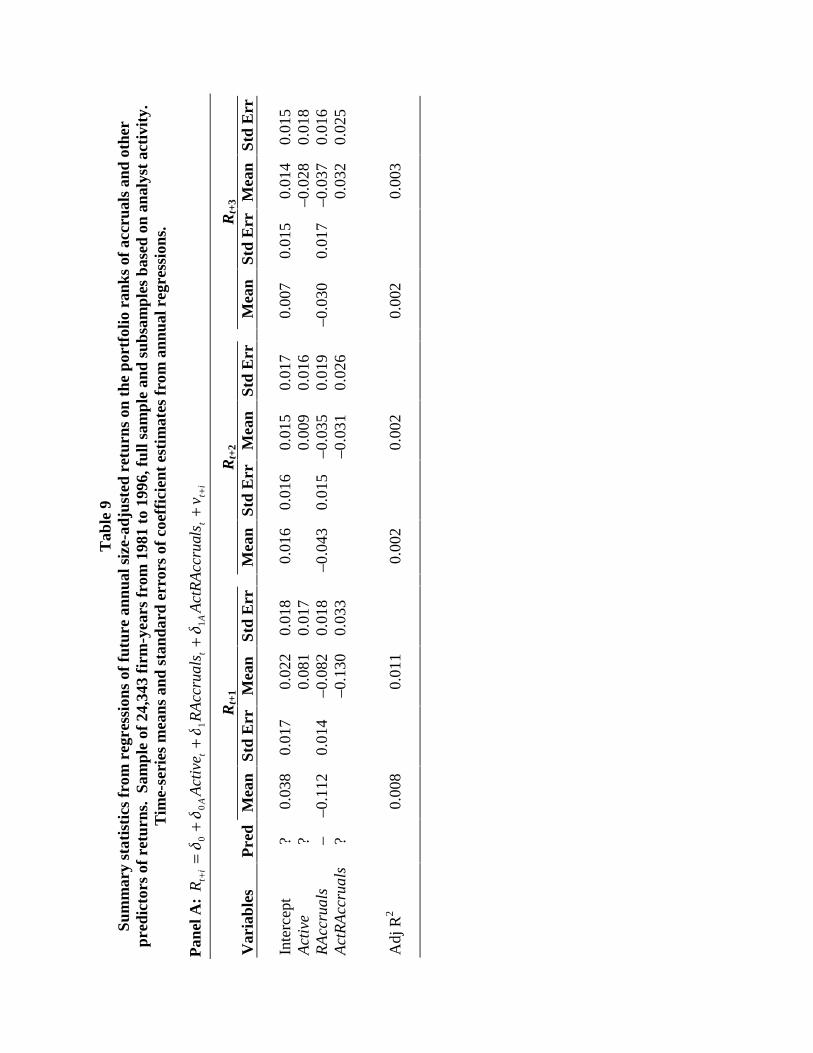
Tab

le 9

Su

mm

ary

stat

isti

cs f

rom

reg

ress

ions

of

futu

re a

nnua

l siz

e-ad

just

ed r

etur

ns o

n th

e po

rtfo

lio r

anks

of

accr

uals

and

oth

er

pred

icto

rs o

f re

turn

s. S

ampl

e of

24,

343

firm

-yea

rs f

rom

198

1 to

199

6, f

ull s

ampl

e an

d su

bsam

ples

bas

ed o

n an

alys

t ac

tivi

ty.

Tim

e-se

ries

mea

ns a

nd s

tand

ard

erro

rs o

f co

effi

cien

t es

tim

ates

fro

m a

nnua

l reg

ress

ions

.

Pan

el A

: i

tt

At

tA

it

vls

Act

RA

ccru

aR

Acc

rual

sA

ctiv

eR

++

++

++

=1

10

0δ

δδ

δ

R

t+1

R

t+2

R

t+3

Var

iabl

es

Pre

d M

ean

Std

Err

M

ean

Std

Err

Mea

n St

d E

rr

Mea

n St

d E

rr

M

ean

Std

Err

M

ean

Std

Err

Inte

rcep

t ?

0.03

8 0.

017

0.02

2 0.

018

0.

016

0.01

6 0.

015

0.01

7

0.00

7 0.

015

0.01

4 0.

015

Act

ive

?

0.

081

0.01

7

0.00

9 0.

016

–0

.028

0.

018

RA

ccru

als

– –0

.112

0.

014

–0.0

82

0.01

8

–0.0

43

0.01

5 –0

.035

0.

019

–0

.030

0.

017

–0.0

37

0.01

6 A

ctR

Acc

rual

s ?

–0.1

30

0.03

3

–0.0

31

0.02

6

0.03

2 0.

025

Adj

R2

0.

008

0.

011

0.00

2

0.00

2

0.

002

0.

003

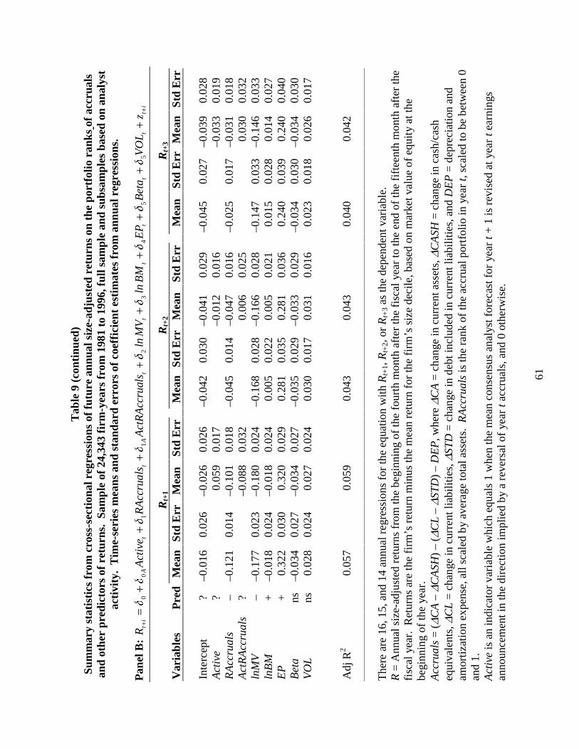
61

Tab

le 9

(co

ntin

ued)

Su

mm

ary

stat

isti

cs f

rom

cro

ss-s

ecti

onal

reg

ress

ions

of f

utur

e an

nual

siz

e-ad

just

ed r

etur

ns o

n th

e po

rtfo

lio r

anks

of

accr

uals

an

d ot

her

pred

icto

rs o

f re

turn

s. S

ampl

e of

24,

343

firm

-yea

rs f

rom

198

1 to

199

6, f

ull s

ampl

e an

d su

bsam

ples

bas

ed o

n an

alys

t ac

tivi

ty.

Tim

e-se

ries

mea

ns a

nd s

tand

ard

erro

rs o

f co

effi

cien

t es

tim

ates

fro

m a

nnua

l reg

ress

ions

.

Pan

el B

: i

tt

tt

tt

tA

tt

Ai

tz

VO

LB

eta

EP

BM

lnM

Vln

lsA

ctR

Acc

rua

RA

ccru

als

Act

ive

R+

++

++

++

++

++

=5

54

32

11

00

δδ

δδ

δδ

δδ

δ

R

t+1

R

t+2

R

t+3

Var

iabl

es

Pre

d M

ean

Std

Err

M

ean

Std

Err

Mea

n St

d E

rr

Mea

n St

d E

rr

M

ean

Std

Err

M

ean

Std

Err

In

terc

ept

? –0

.016

0.

026

–0.0

26

0.02

6

–0.0

42

0.03

0 –0

.041

0.

029

–0

.045

0.

027

–0.0

39

0.02

8 A

ctiv

e ?

0.05

9 0.

017

–0

.012

0.

016

–0

.033

0.

019

RA

ccru

als

– –0

.121

0.

014

–0.1

01

0.01

8

–0.0

45

0.01

4 –0

.047

0.

016

–0

.025

0.

017

–0.0

31

0.01

8 A

ctR

Acc

rual

s ?

–0.0

88

0.03

2

0.00

6 0.

025

0.

030

0.03

2 ln

MV

–

–0.1

77

0.02

3 –0

.180

0.

024

–0

.168

0.

028

–0.1

66

0.02

8

–0.1

47

0.03

3 –0

.146

0.

033

lnB

M

+

–0.0

18

0.02

4 –0

.018

0.

024

0.

005

0.02

2 0.

005

0.02

1

0.01

5 0.

028

0.01

4 0.

027

EP

+

0.

322

0.03

0 0.

320

0.02

9

0.28

1 0.

035

0.28

1 0.

036

0.

240

0.03

9 0.

240

0.04

0 B

eta

ns

–0.0

34

0.02

7 –0

.034

0.

027

–0

.035

0.

029

–0.0

33

0.02

9

–0.0

34

0.03

0 –0

.034

0.

030

VO

L

ns

0.02

8 0.

024

0.02

7 0.

024

0.

030

0.01

7 0.

031

0.01

6

0.02

3 0.

018

0.02

6 0.

017

A

dj R

2

0.05

7

0.05

9

0.

043

0.

043

0.04

0

0.04

2

T

here

are

16,

15,

and

14

annu

al r

egre

ssio

ns f

or th

e eq

uatio

n w

ith R

t+1,

Rt+

2, o

r R

t+3

as th

e de

pend

ent v

aria

ble.

R

= A

nnua

l siz

e-ad

just

ed r

etur

ns f

rom

the

begi

nnin

g of

the

four

th m

onth

aft

er th

e fi

scal

yea

r to

the

end

of th

e fi

ftee

nth

mon

th a

fter

the

fisc

al y

ear.

Ret

urns

are

the

firm

’s r

etur

n m

inus

the

mea

n re

turn

for

the

firm

’s s

ize

deci

le, b

ased

on

mar

ket v

alue

of

equi

ty a

t the

be

ginn

ing

of th

e ye

ar.

A

ccru

als

= (

∆CA

– ∆

CA

SH)

– (∆

CL

– ∆

STD

) –

DE

P, w

here

∆C

A =

cha

nge

in c

urre

nt a

sset

s, ∆

CA

SH =

cha

nge

in c

ash/

cash

eq

uiva

lent

s, ∆

CL

= c

hang

e in

cur

rent

liab

ilit

ies,

∆ST

D =

cha

nge

in d

ebt i

nclu

ded

in c

urre

nt li

abili

ties,

and

DE

P =

dep

reci

atio

n an

d am

orti

zati

on e

xpen

se, a

ll sc

aled

by

aver

age

tota

l ass

ets.

RA

ccru

als

is th

e ra

nk o

f th

e ac

crua

l por

tfol

io in

yea

r t,

scal

ed to

be

betw

een

0 an

d 1.

A

ctiv

e is

an

indi

cato

r va

riab

le w

hich

equ

als

1 w

hen

the

mea

n co

nsen

sus

anal

yst f

orec

ast f

or y

ear

t + 1

is r

evis

ed a

t yea

r t e

arni

ngs

anno

unce

men

t in

the

dire

ctio

n im

plie

d by

a r

ever

sal o

f ye

ar t

accr

uals

, and

0 o

ther

wis

e.

62

Act

RA

ccru

als

= A

ctiv

e ×

RA

ccru

als.

ln

MV

= n

atur

al lo

gari

thm

of

the

mar

ket v

alue

of

equi

ty.

ln

BM

= n

atur

al lo

gari

thm

of

the

book

-to-

mar

ket r

atio

.

EP

= th

e ea

rnin

gs-t

o-pr

ice

ratio

.

Bet

a =

bet

a ob

tain

ed f

rom

CR

SP.

V

OL

= a

nnua

l tra

ding

vol

ume

divi

ded

by s

hare

s ou

tsta

ndin

g.

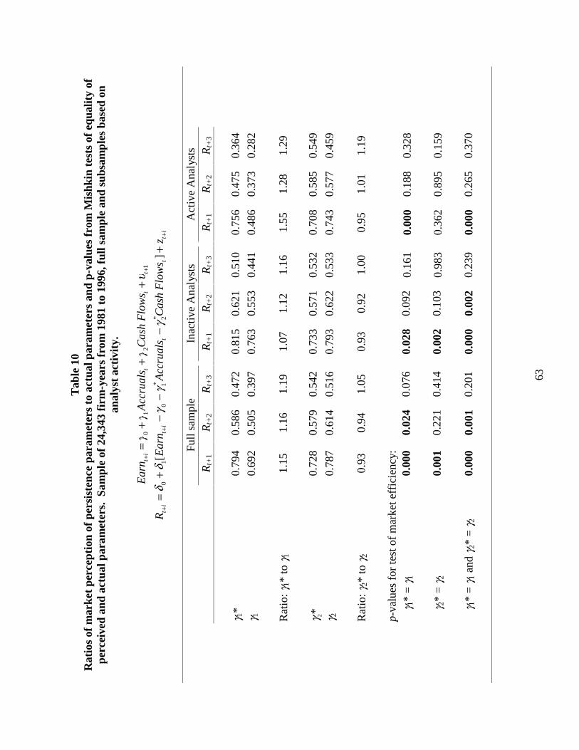
63

Tab

le 1

0 R

atio

s of

mar

ket

perc

epti

on o

f pe

rsis

tenc

e pa

ram

eter

s to

act

ual p

aram

eter

s an

d p-

valu

es f

rom

Mis

hkin

tes

ts o

f eq

ualit

y of

pe

rcei

ved

and

actu

al p

aram

eter

s. S

ampl

e of

24,

343

firm

-yea

rs f

rom

198

1 to

199

6, f

ull s

ampl

e an

d su

bsam

ples

bas

ed o

n an

alys

t ac

tivi

ty.

12

10

+

++

++

=t

tt

it

Flo

ws

Cas

hA

ccru

als

Ear

nυ

γγ

γ

it

tt

it

it

zF

low

sC

ash

Acc

rual

sE

arn

R+

++

+−

−−

+=

]

[* 2

* 10

10

γγ

γδ

δ

Full

sam

ple

In

activ

e A

naly

sts

A

ctiv

e A

naly

sts

R

t+1

Rt+

2 R

t+3

R

t+1

Rt+

2 R

t+3

R

t+1

Rt+

2 R

t+3

γ 1*

0.79

4 0.

586

0.47

2

0.81

5 0.

621

0.51

0

0.75

6 0.

475

0.36

4

γ 1

0.69

2 0.

505

0.39

7

0.76

3 0.

553

0.44

1

0.48

6 0.

373

0.28

2

Rat

io: γ

1* to

γ 1

1.15

1.

16

1.19

1.07

1.

12

1.16

1.55

1.

28

1.29

γ 2*

0.72

8 0.

579

0.54

2

0.73

3 0.

571

0.53

2

0.70

8 0.

585

0.54

9

γ 2

0.78

7 0.

614

0.51

6

0.79

3 0.

622

0.53

3

0.74

3 0.

577

0.45

9

Rat

io: γ

2* to

γ 2

0.93

0.

94

1.05

0.93

0.

92

1.00

0.95

1.

01

1.19

p-

valu

es f

or te

st o

f m

arke

t eff

icie

ncy:

γ 1*

= γ 1

0.

000

0.02

4 0.

076

0.

028

0.09

2 0.

161

0.

000

0.18

8 0.

328

γ 2

* =

γ 2

0.00

1 0.

221

0.41

4

0.00

2 0.

103

0.98

3

0.36

2 0.

895

0.15

9

γ 1*

= γ 1

and

γ 2*

= γ 2

0.

000

0.00

1 0.

201

0.

000

0.00

2 0.

239

0.

000

0.26

5 0.

370

64

Ear

n =

ear

ning

s fr

om c

ontin

uing

ope

ratio

ns a

fter

dep

reci

atio

n, s

cale

d by

ave

rage

tota

l ass

ets.

C

ashF

low

s =

Ear

n –

Acc

rual

s.

Acc

rual

s =

(∆C

A –

∆C

ASH

) –

(∆C

L –

∆ST

D)

– D

EP

, whe

re ∆

CA

= c

hang

e in

cur

rent

ass

ets,

∆C

ASH

= c

hang

e in

cas

h/ca

sh

equi

vale

nts,

∆C

L =

cha

nge

in c

urre

nt li

abil

itie

s, ∆

STD

= c

hang

e in

deb

t inc

lude

d in

cur

rent

liab

ilitie

s, a

nd D

EP

= d

epre

ciat

ion

and

amor

tiza

tion

exp

ense

, all

scal

ed b

y av

erag

e to

tal a

sset

s.

R =

Ann

ual s

ize-

adju

sted

ret

urns

fro

m th

e be

ginn

ing

of th

e fo

urth

mon

th a

fter

the

fisc

al y

ear

to th

e en

d of

the

fift

eent

h m

onth

aft

er th

e fi

scal

yea

r. R

etur

ns a

re th

e fi

rm’s

ret

urn

min

us th

e m

ean

retu

rn f

or th

e fi

rm’s

siz

e de

cile

, bas

ed o

n m

arke

t val

ue o

f eq

uity

at t

he

begi

nnin

g of

the

year

.