RESEARCH OpenAccess …RESEARCH OpenAccess Statemodellingofthelandmobile...

Arndt et al. EURASIP Journal onWireless Communications and Networking 2012, 2012:228http://jwcn.eurasipjournals.com/content/2012/1/228

RESEARCH Open Access

State modelling of the land mobilepropagation channel for dual-satellite systemsDaniel Arndt1*, Alexander Ihlow1, Thomas Heyn2, Albert Heuberger2, Roberto Prieto-Cerdeira3

and Ernst Eberlein2

Abstract

The quality of service of mobile satellite reception can be improved by using multi-satellite diversity (angle diversity).The recently finalised MiLADY project targeted therefore on the evaluation and modelling of the multi-satellitepropagation channel for land mobile users with focus on broadcasting applications. The narrowband modelcombines the parameters from two measurement campaigns: In the U.S. the power levels of the Satellite DigitalAudio Radio Services were recorded with a high sample rate to analyse fast and slow fading effects in great detail. In acomplementary campaign signals of Global Navigation Satellite Systems (GNSS) were analysed to obtain informationabout the slow fading correlation for almost any satellite constellation. The new channel model can be used togenerate time series for various satellite constellations in different environments. This article focuses on realistic statesequence modelling for angle diversity, confining on two satellites. For this purpose, different state modellingmethods providing a joint generation of the states ‘good good’, ‘good bad’, ‘bad good’ and ‘bad bad’ are compared.Measurements and re-simulated data are analysed for various elevation combinations and azimuth separations interms of the state probabilities, state duration statistics, and correlation coefficients. The finally proposed state modelis based on semi-Markov chains assuming a log-normal state duration distribution.

Keywords: Land mobile satellite, Statistical propagation model, Satellite diversity, Markov chain, Semi-Markov chain

1 IntroductionSatellites play an important role in today’s commer-cial broadcasting systems. In cooperation with terres-trial repeaters they can ensure uninterrupted service ofmultimedia content (e.g. audio and video streaming) tostationary, portable, and mobile receivers. However, incase of mobile reception fading regularly disrupts the sig-nal transmission due to shadowing or blocking objectsbetween satellite and receiver. To mitigate these fadingeffects, diversity techniques such as angle diversity (mul-tiple satellites) and time diversity (interleaving) are attrac-tive. For link-level studies of the land mobile satellite(LMS) channel, statistical channel models are frequentlyused that are able to generate timeseries of the receivedfading signal. Statistical LMS channel models describeseveral fading processes of the received signal: slow vari-ations of the signal are caused by obstacles between the

*Correspondence: [email protected] University of Technology, Ilmenau, GermanyFull list of author information is available at the end of the article

satellite and the receiver, which induce varying shadow-ing conditions of the direct signal component. Fast signalvariations are caused by multipath effects due to staticor moving scatterers in the vicinity of the mobile termi-nal. For short time periods these two components (slowand fast variations) are usually modelled by a station-ary stochastic processes, e.g., as a Loo-distributed fadingsignal [1]. For longer time periods the received signalcan not assumed to be stationary. Therefore, statisticalLMS channel models describe different receive states toassess the large dynamic range of the received signal. Thestates correspond to slow varying environmental condi-tions (e.g. line of trees, buildings, line-of-sight (LOS)) inthe transmission path. Traditional LMS channel modelssimulate series of three states (‘line-of-sight’, ‘shadowed’,and ‘blocked’) or two states (‘good’ state and ‘bad’ state) byusing Markov or semi-Markov concepts.While several LMS channel models for single-satellite

systems are already available and consolidated [2-4],models for multi-satellites systems are of ongoing interestfor modern transmission standards, e.g. DVB-SH [5].

© 2012 Arndt et al.; licensee Springer. This is an Open Access article distributed under the terms of the Creative CommonsAttribution License (http://creativecommons.org/licenses/by/2.0), which permits unrestricted use, distribution, and reproductionin any medium, provided the original work is properly cited.

Arndt et al. EURASIP Journal onWireless Communications and Networking 2012, 2012:228 of 21http://jwcn.eurasipjournals.com/content/2012/1/228

Early studies on multi-satellite transmission were carriedout in 1992. Based on circular scans of fisheye-camerapictures in different environments an empirical modelwas developed describing the correlation coefficientbetween two satellite signals depending on their azimuthseparation [6]. In 1996 a statistical channel model for twocorrelated satellites based on first-order Markov chainswas developed [7]. The state sequence generation is basedon state transition probabilities of two independent satel-lites. Both satellites are combined by a state correlationparameter which can be taken from empirical models.Due to its simplicity this modelling approach is frequentlyused today. However, first-order Markov chains have limi-tations in state durationmodelling, as their state durationsfollow an exponential distribution. Studies in [8-10] foundthat this condition does not hold for the LMS channel.Nevertheless, a correct state duration modelling is of highinterest for the optimal configuration of physical layerand link layer parameters for modern broadcasting stan-dards with long time interleaving (e.g. for physical layerinterleaver size, link layer protection time). Therefore,different concepts improving the state duration modellingwere introduced: semi-Markov chains [10] and dynamicMarkov chains [9]. For these approaches some exemplaryparameters for the single-satellite reception are pub-lished. However, an intense study for multi-satellite stateduration modelling and a corresponding channel modelincluding parameters for different environments andorbital positions does not exist so far. In this sense, a newchannel model for two or more satellites was developedin the context of the project MiLADY (Mobile satellitechanneL with Angle DiversitY ) [11]. This project coveredtwo measurement campaigns in the U.S. and in Europe: Inthe first campaign the power levels of the Satellite DigitalAudio Radio Services (SDARS) satellites (S-Band) wererecorded synchronously with a sample rate of 2.1 kHz.The signals allow to study slow and fast fading effectsin combination with angle diversity for a limited set ofelevation and azimuth angle combinations. A secondmeasurement campaign was carried out in the area ofErlangen in Germany to record the carrier-to-noise spec-tral density ratio (C/N0) from Global Navigation SatelliteSystem (GNSS) satellites in the L-Band. The C/N0 allowsa comprehensive analysis of the state correlation (line ofsight, shadowed/blocked) for multiple satellites for a widerange of elevation and azimuth angle combinations.This article focuses on the state sequence generation

for a dual-satellite channel model. The parameters arederived from the measurements for different modellingapproaches assuming two states per satellite (‘good’,‘bad’). Chosen models are: first-order Markov approach[7], semi-Markov approach [10], and dynamic Markovapproach [9]. To assess the performance of these models,correlation coefficients, state probabilities and state

duration statistics are gained from re-simulated statesequences and compared with the measurement data. Asstate sequence modelling is only a part of a completeLMS channel model, we describe an overall LMS channelmodel and give the complete set of parameters.The article is organised as follows: In Section 2 basics of

the LMS channel and of different state modelling methodsfor single- and dual-satellite reception are explained. Fur-ther on, these methods are compared on an exemplaryscenario for two satellites. Section 3 gives an overview onthe GNSS and SDARS measurements and the data pro-cessing to derive the channel states. In Section 4 the statemodels are compared on a high number of receive sce-narios with the measurements. The evaluation criteria arestate probabilities and state duration statistics. Finally, inSection 5 the conclusions are drawn.

2 Statistical channel modelling for single-satelliteand dual-satellite systems

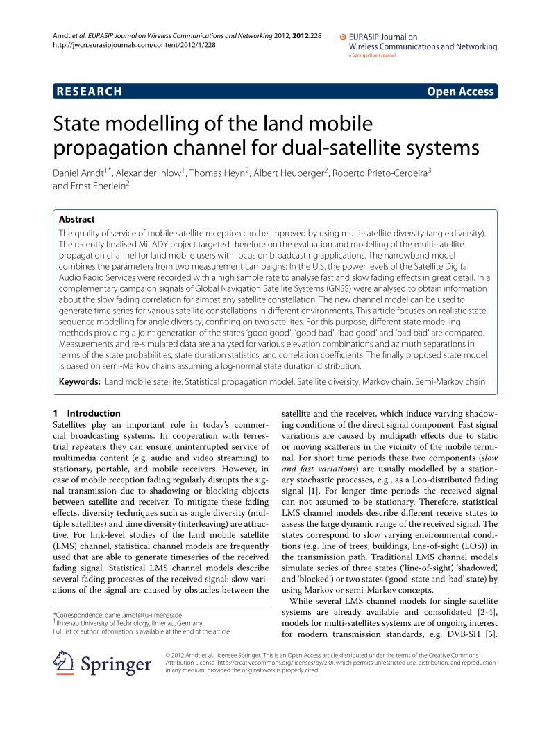
The statistical approach of generating time series for theLMS propagation channel includes two processes: First,the very slow fading components of the channel due tovarying shadowing conditions between the satellite andthe receiver are modelled in terms of channel states.LMS models with three states [3], namely ‘line-of-sight’,‘shadowed’, and ‘blocked’, or two states [2,4] ‘good’ and‘bad’ are available in the literature. Once the channelstates are modelled, in a second process the amplitudesof direct and indirect signal components are generated.They depend on the current state and the receive environ-ment. In common narrowband LMS propagation modelsthe fading is described as a combination of log-normal,Rice and Rayleigh models.In Figure 1 the two-state approach according to Prieto-

Cerdeira et al. [4] is illustrated. This model describestwo states: a ‘good’ state (corresponding to LOS/lightshadowing), and a ‘bad’ state (corresponding to heavyshadowing/blockage). Within each state a Loo-distributedfading signal [1] is assumed. It includes a slow fadingcomponent (lognormal fading) corresponding to varyingshadowing conditions of the direct signal, and a fast fad-ing component due to multipath effects. The Loo modelis described by three parametersMA, �A, andMP, denot-ing the mean and standard deviation of the lognormalcomponent, and the multipath power, respectively. Aftereach state transition a random Loo parameter triplet isgenerated following a statistical distribution. The distribu-tion of the Loo parameter triplets depends on the currentstate, and further on the receive environment of the ter-minal. This two-state model is an evolution of an earlierthree-state model [3], where the Loo parameter triplet foreach state was fixed within a given environment and ele-vation. The versatile Loo parameter selection of the newermodel enables a more realistic modelling over the full


slow variations

fast variations

good state

bad state

travelled distance [m]

sign

alle

vel[

dB]

very slow variations = states( A, A, MP) i

( A, A, MP) i+1

( A, A, MP) i+2

( A, A, MP) i+3

Figure 1 Signal components of a two-state LMS channel model.

dynamic range of the received signal. Therefore, the two-state model from Prieto-Cerdeira et al. [4] was extendedfor the new multi-satellite narrowband model developedwithin the MiLADY project.Focus of this article is the state sequence modelling for

single- and dual-satellite systems, assuming two states persatellite: ‘good’ state and ‘bad’ state. For this purpose, dif-ferent state modelling methods are compared with themeasurement data in terms of the state probability, stateduration probability, and correlation coefficient. More-over the practicability of various state generation methodsin terms of generating a database, e.g. for different envi-ronments and elevation angles, is assessed.

2.1 Channel state models for single-satellite systemsThree types of state modelling approaches for single-satellite systems are found in the literature:

• First-order Markov model [3]• Dynamic Markov model [9]• Semi-Markov model [10]

In the following themain characteristics of thesemodelsare described.

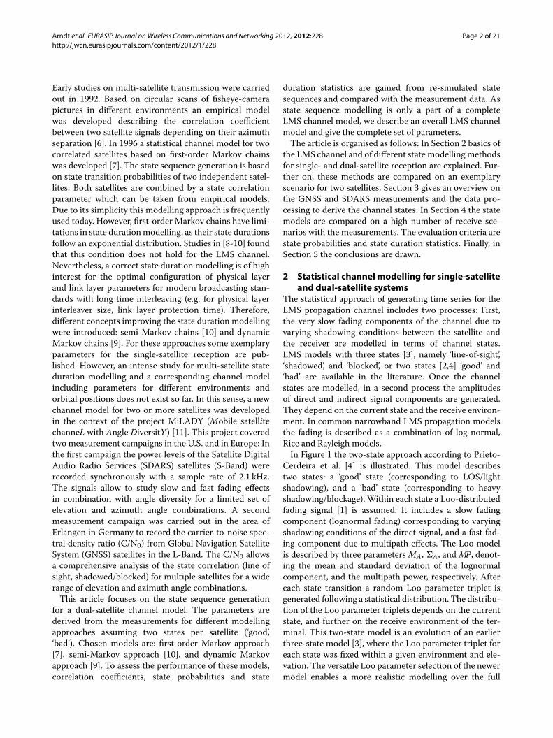
2.1.1 First-order MarkovmodelA Markov model is a special random process for generat-ing discrete samples corresponding to channel states s of apredefined sample length. For a first-order Markov model,each state depends only on the previous state. The con-ditional probabilities of state sn+1 given the state sn aredescribed by state transition probabilities pij. Therefore,the only parameter of the Markov chain is the state tran-sition probability matrix (STPM) Ptrans ∈ R

N×N0+ with N

being the number of states (cf. Figure 2a). The main char-acteristic of a first-order Markov chain is, that it enablesan exact modelling of the state probability and the averagestate duration. It satisfies

p·[Ptrans − I]= 0 (1)

with p being the row vector of the equilibrium stateprobabilities, the unity matrix I, and the zero vector 0.The average state duration is calculated by

D = 11 − pii

· 1�d

, (2)

state duration pdfof Good state

Good#1

Bad#2

p21

p12

p22p11

Good#1

Bad#2

p22(n2)

Good#1

Bad#2

p21 =1

p12 =1

state duration pdfof Bad state

p21(n2)

p12(n1)

p11(n1)

a

b

c

Figure 2 Single-satellite state models assuming two states. (a)First-order Markov model. (b) Dynamic Markov model. (c)Semi-Markov model.


where pii is the state transition probability between twoequal states, and�d denotes the sampling distance (framelength).The probability that the Markov chain stays in state i for

n consecutive samples is given by

Pi(D = n�d) = pn−1ii · (1 − pii), n ∈ N , (3)

In this article the function P(D) will be further denotedas state duration probability density function (SDPDF).The SDPDF of the first-order Markov chain follows anexponential distribution.

2.1.2 DynamicMarkovmodelResults in [9,10] have shown that an exponential SDPDFis no accurate approximation for the LMS channel. There-fore, to improve the state duration modelling dynamicMarkov chains were introduced [9]. For dynamic Markovchains the state transition probability is a function of thecurrent state duration n (cf. Figure 2b)

pij = f (n) . (4)

For this purpose, the two-dimensional STPM isextended to a three-dimensional state transition proba-bility tensor (STPT) Ptrans ∈ R

N×N×nmax0+ , where nmax

corresponds to the maximum state length obtained fromthe measurements with Dmax = nmax�d.Using the dynamic Markov model, the probability that

the state duration is equal to D is

Pi(D = n�d) = (1−pii(n�d))·n−1∏r=1

pii(r�d), n ∈ N .

(5)

If the values for the STPT are directly derived from themeasured state sequence (assuming a sample length of e.g.�d = 1m), the dynamic Markov model enables an exactreproduction of the state probabilities as well as an exactre-modelling of the measured SDPDF. A significant dis-advantage is the high number of parameters required todescribe the STPT.In [9] some model approximations are proposed to

reduce the number of required parameters of the STPT:

• partial dynamic Markov model: From Equation (5) itis derived that an exact state duration modellingrequires only a subset of the STPT. Only thetransition coefficients pii(n) need to change as afunction of the current state duration. For a two-statemodel the remaining values pij(n) can be recalculatedeasily with pij(n) + pii(n) = 1. For a multi-statemodel some additional coefficients SiZ are required tocalculate the relative ratio between the state transitionprobabilities pij(n). The coefficients are derived fromthe STPT Ptrans at position n = 1 for each state i

pii(1) + Si1(1) + Si2(1) + · · · + SiZ(1) = 1 , withSiZ(1) = pij(1), i �= j. (6)

Then, to calculate the relative coefficients at positionspij(n > 1) it holds:

pii(n)+kSi1+kSi2+· · ·+kSiZ =1 , with kSiZ =pij(n).(7)

• approximated partial dynamic Markov model: For afurther reduction of the model parameters, thefunction pii(n) can be approximated by a curve fit. In[9], a piecewise linear approximation at 8 predefinedvalues of the state duration D = n�d is proposed.Assuming this, a two-state model would require 8 · 2parameters for state sequence generation. Amulti-state model would need 8 · N parameters todescribe the functions pii(n) (with N being thenumber of states) and further N(N − 1) parametersto describe the relative ratios SiZ between thecoefficients pij(n), i �= j (Equation (6)).

2.1.3 Semi-MarkovmodelAnother Markov approach is the semi-Markov modelintroduced in [10] to enable a correct state duration mod-elling. In contrast to the first-order- and dynamic Markovmodel, the state transitions do not occur at concrete timeintervals. In fact, the time interval of the model staying instate i depends directly on its SDPDF. As with the Markovmodels, the state transitions are described with the statetransition probability pij, but with i �= j. Assuming asingle-satellite model of only two states, the state transi-tion probability is pij = 1 (cf. Figure 2c). The equilibriumprobability of the states can be calculated as the product ofthe mean state duration D and the probability of enteringa state (which is described with the STPM).The semi-Markov model offers some options to

describe the SDPDF of each state:

• The measured state duration statistic is used withoutany approximation for re-modelling, i.e., the stateduration is a random realisation of the measuredSDPDF.

P(D) = P(Dmeasured) (8)• The measured SDPDF is approximated with a log-

normal distribution, as proposed in [4,10] individuallyfor the single-satellite state ‘good’ and ‘bad’. Thelognormal probability density function describing thestate duration probability P(D) is given by

P(D) = 1Dσ

√2π

exp[− (ln(D) − μ)2

2σ 2

], (9)

where σ is the standard deviation of ln(D) and μ isthe mean value of ln(D). Using this approximation,only two parameters per state are required to


describe the SDPDF. The mean state duration D canbe calculated with

D = exp[μ + 0.5σ 2] . (10)

• In [9], a piecewise exponential curve fit of the SDPDFusing four segments is proposed. Clearly, thisrequires more parameters than the lognormal curvefit, but it enables a more flexible re-modelling of thestate duration statistic.

P(D) =

⎧⎪⎪⎨⎪⎪⎩

a1 e−b1D , D0 ≤ D ≤ D1a2 e−b2D , D1 ≤ D ≤ D2a3 e−b3D , D2 ≤ D ≤ D3a4 e−b4D , D3 ≤ D ≤ D4

(11)

In any case, the STPM has to be derived from mea-surements, which is independent from the used SDPDFapproximation.

State probability and mean state durations of semi-Markov chains: In some cases, an approximation of thestate duration with a lognormal distribution or a piecewisecurve fit changes the mean state length and consequentlythe total probability of the states. To enable an exactdescription of D and P anyway, a correction of the curvefit can be implemented. For example: for the lognormal fitthe parameter μ can be modified with

μcorrected = ln[Dmeasuredexp(0.5σ 2)

]. (12)

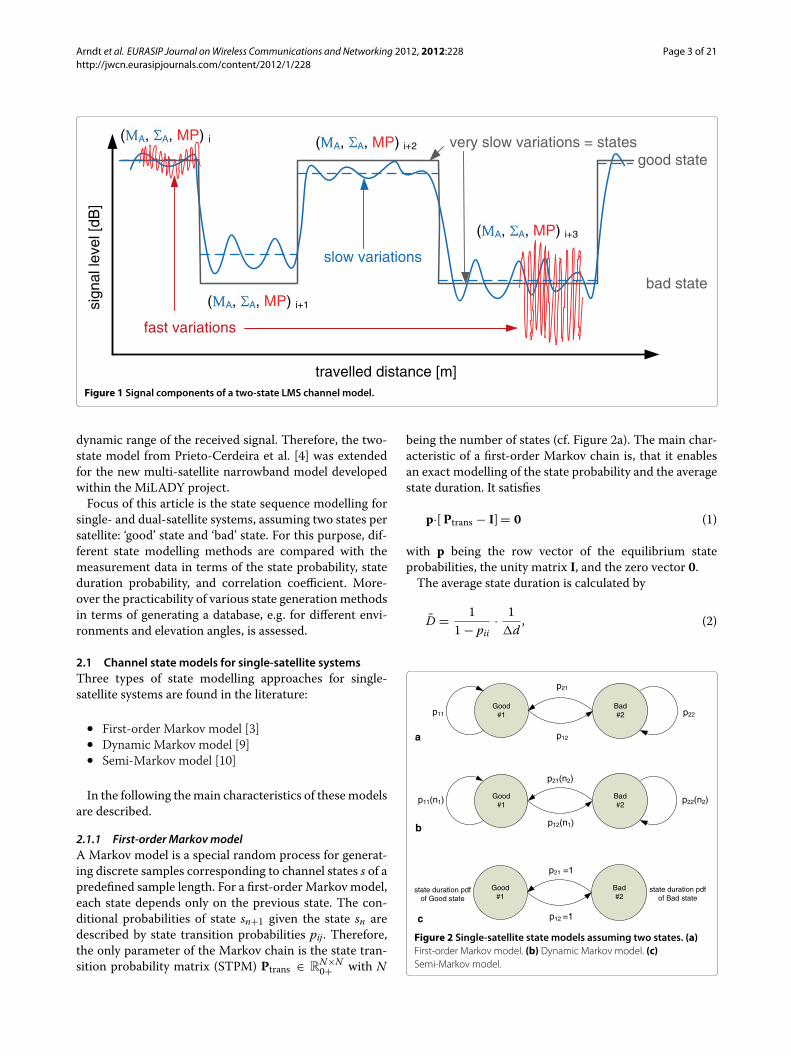
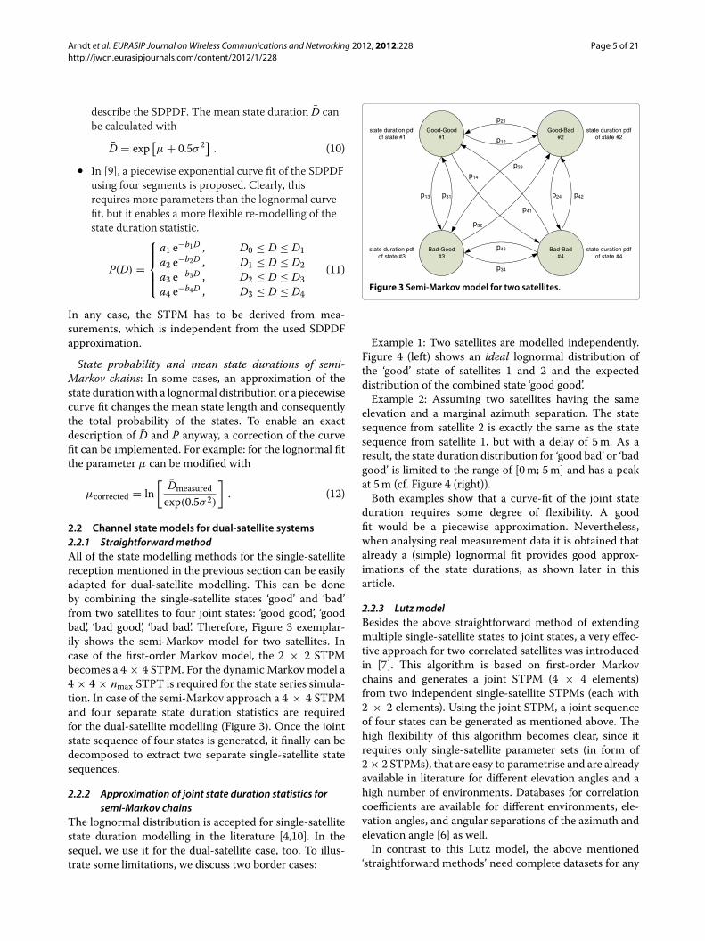
2.2 Channel state models for dual-satellite systems2.2.1 StraightforwardmethodAll of the state modelling methods for the single-satellitereception mentioned in the previous section can be easilyadapted for dual-satellite modelling. This can be doneby combining the single-satellite states ‘good’ and ‘bad’from two satellites to four joint states: ‘good good’, ‘goodbad’, ‘bad good’, ‘bad bad’. Therefore, Figure 3 exemplar-ily shows the semi-Markov model for two satellites. Incase of the first-order Markov model, the 2 × 2 STPMbecomes a 4 × 4 STPM. For the dynamic Markov model a4 × 4 × nmax STPT is required for the state series simula-tion. In case of the semi-Markov approach a 4 × 4 STPMand four separate state duration statistics are requiredfor the dual-satellite modelling (Figure 3). Once the jointstate sequence of four states is generated, it finally can bedecomposed to extract two separate single-satellite statesequences.

2.2.2 Approximation of joint state duration statistics forsemi-Markov chains

The lognormal distribution is accepted for single-satellitestate duration modelling in the literature [4,10]. In thesequel, we use it for the dual-satellite case, too. To illus-trate some limitations, we discuss two border cases:

Good-Good#1

Bad-Bad#4

Good-Bad#2

Bad-Good#3

p12

p21

p43

p34

p42p24p13 p31

p23

p32

p41

p14

state duration pdfof state #2




Figure 3 Semi-Markov model for two satellites.

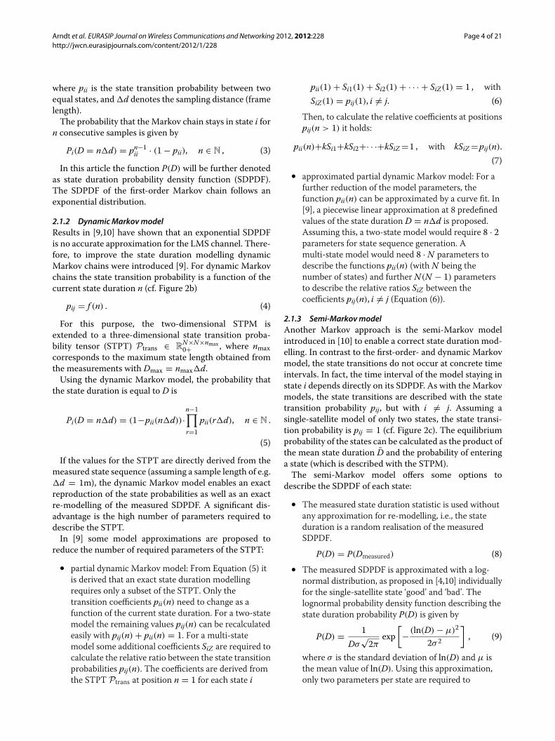
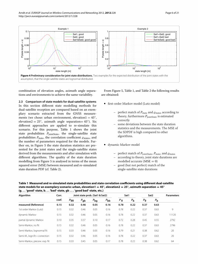
Example 1: Two satellites are modelled independently.Figure 4 (left) shows an ideal lognormal distribution ofthe ‘good’ state of satellites 1 and 2 and the expecteddistribution of the combined state ‘good good’.Example 2: Assuming two satellites having the same

elevation and a marginal azimuth separation. The statesequence from satellite 2 is exactly the same as the statesequence from satellite 1, but with a delay of 5m. As aresult, the state duration distribution for ‘good bad’ or ‘badgood’ is limited to the range of [0m; 5m] and has a peakat 5m (cf. Figure 4 (right)).Both examples show that a curve-fit of the joint state

duration requires some degree of flexibility. A goodfit would be a piecewise approximation. Nevertheless,when analysing real measurement data it is obtained thatalready a (simple) lognormal fit provides good approx-imations of the state durations, as shown later in thisarticle.

2.2.3 LutzmodelBesides the above straightforward method of extendingmultiple single-satellite states to joint states, a very effec-tive approach for two correlated satellites was introducedin [7]. This algorithm is based on first-order Markovchains and generates a joint STPM (4 × 4 elements)from two independent single-satellite STPMs (each with2 × 2 elements). Using the joint STPM, a joint sequenceof four states can be generated as mentioned above. Thehigh flexibility of this algorithm becomes clear, since itrequires only single-satellite parameter sets (in form of2 × 2 STPMs), that are easy to parametrise and are alreadyavailable in literature for different elevation angles and ahigh number of environments. Databases for correlationcoefficients are available for different environments, ele-vation angles, and angular separations of the azimuth andelevation angle [6] as well.In contrast to this Lutz model, the above mentioned

‘straightforward methods’ need complete datasets for any


Figure 4 Preliminary consideration for joint state distributions. Two examples for the expected distribution of the joint states with theassumption, that the single satellite states are lognormal distributed.

combination of elevation angles, azimuth angle separa-tions and environments to achieve the same variability.

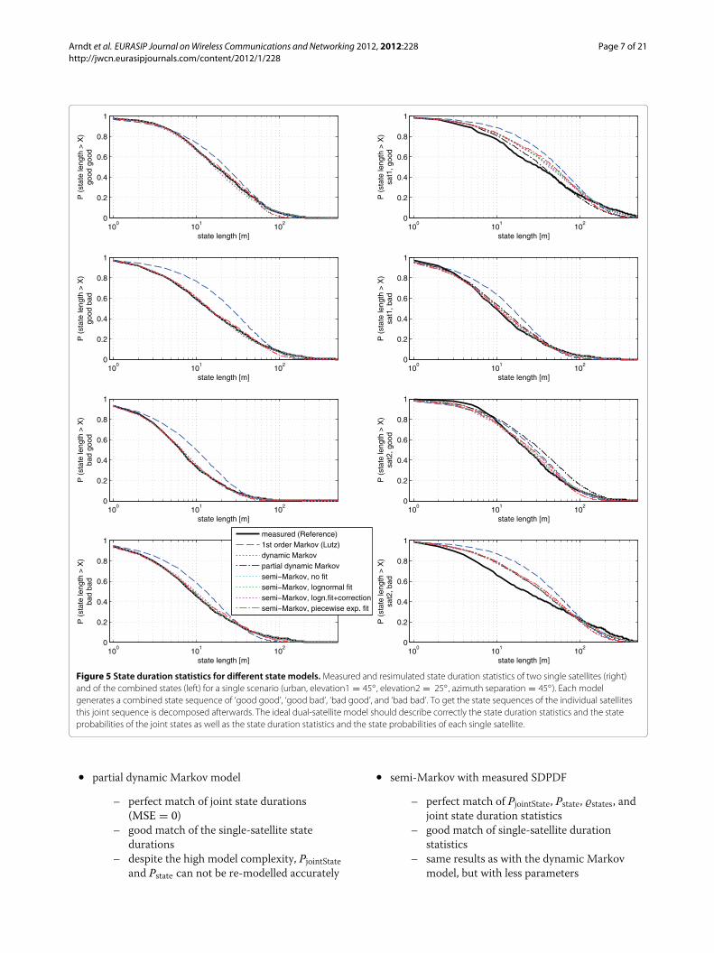
2.3 Comparison of state models for dual-satellite systemsIn this section different state modelling methods fordual-satellite reception are compared based on an exem-plary scenario extracted from the GNSS measure-ments (we chose: urban environment, elevation1 = 45◦,elevation2 = 25◦, azimuth angle separation= 45◦). Sixdifferent approaches are applied to re-simulate thisscenario. For this purpose, Table 1 shows the jointstate probabilities PjointState, the single-satellite stateprobabilities Pstate, the correlation coefficient �states, andthe number of parameters required for the models. Fur-ther on, in Figure 5 the state duration statistics are pre-sented for the joint states and the single-satellite statesderived from the measurements and after simulation withdifferent algorithms. The quality of the state durationmodelling from Figure 5 is analysed in terms of the meansquared error (MSE) between measured and re-simulatedstate duration PDF (cf. Table 2).

From Figure 5, Table 1, and Table 2 the following resultsare obtained:

• first-order Markov model (Lutz model)

– perfect match of Pstate and �states according totheory, furthermore PjointState is estimatedcorrectly

– some deviations between the state durationstatistics and the measurements. The MSE ofthe SDPDF is high compared to otheralgorithms.

• dynamic Markov model

– perfect match of PjointState, Pstate, and �states– according to theory, joint state durations are

modelled accurate (MSE = 0)– good (but not perfect) match of the

single-satellite state durations

Table 1 Measured and re-simulated state probabilities and state correlation coefficients using different dual-satellitestate models for an exemplary scenario: urban, elevation1 = 45◦, elevation2 = 25◦, azimuth separation = 45◦(g. . . ‘good’-state, b. . . ‘bad’-state, gb . . . ‘good bad’-state, etc.)

Algorithm Corr. Joint state prob. (Sat1& Sat2) Sat1 Sat2 Parameters

coef. Pgg Pgb Pbg Pbb Pg Pb Pg Pbmeasured (Reference) 0.15 0.32 0.46 0.05 0.16 0.78 0.22 0.37 0.63

1st order Markov (Lutz) 0.15 0.32 0.46 0.05 0.16 0.78 0.22 0.37 0.63 9

dynamic Markov 0.15 0.32 0.46 0.05 0.16 0.78 0.22 0.37 0.63 11120

partial dynamic Markov 0.10 0.35 0.37 0.10 0.17 0.72 0.28 0.45 0.55 2792

Semi-Markov, no fit 0.15 0.32 0.46 0.05 0.16 0.78 0.22 0.37 0.63 2796

Semi-Markov, lognormal fit 0.15 0.33 0.46 0.05 0.16 0.79 0.21 0.38 0.62 20

Semi-M., logn.fit + correction 0.15 0.32 0.46 0.05 0.16 0.78 0.22 0.37 0.63 20

Semi-Markov, piecew. exp. fit 0.15 0.33 0.45 0.05 0.17 0.78 0.22 0.38 0.62 64


Figure 5 State duration statistics for different state models.Measured and resimulated state duration statistics of two single satellites (right)and of the combined states (left) for a single scenario (urban, elevation1 = 45◦ , elevation2 = 25◦ , azimuth separation = 45◦). Each modelgenerates a combined state sequence of ‘good good’, ‘good bad’, ‘bad good’, and ‘bad bad’. To get the state sequences of the individual satellitesthis joint sequence is decomposed afterwards. The ideal dual-satellite model should describe correctly the state duration statistics and the stateprobabilities of the joint states as well as the state duration statistics and the state probabilities of each single satellite.

• partial dynamic Markov model

– perfect match of joint state durations(MSE = 0)

– good match of the single-satellite statedurations

– despite the high model complexity, PjointStateand Pstate can not be re-modelled accurately

• semi-Markov with measured SDPDF

– perfect match of PjointState, Pstate, �states, andjoint state duration statistics

– good match of single-satellite durationstatistics

– same results as with the dynamic Markovmodel, but with less parameters


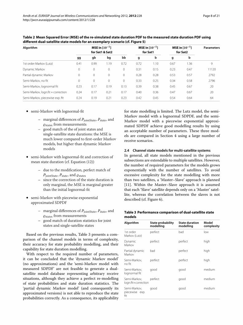
Table 2 Mean Squared Error (MSE) of the re-simulated state duration PDF to themeasured state duration PDF usingdifferent dual-satellite state models for an exemplary scenario (cf. Figure 5)

Algorithm MSE in [10−5] MSE in [10−5] MSE in [10−5] Parametersfor Sat1&Sat2 for Sat1 for Sat2

gg gb bg bb g b g b

1st order Markov (Lutz) 0.41 0.99 1.19 0.72 0.72 1.10 0.67 1.36 9

Dynamic Markov 0 0 0 0 0.31 0.15 0.23 0.47 11120

Partial dynamic Markov 0 0 0 0 0.28 0.28 0.53 0.57 2792

Semi-Markov, no fit 0 0 0 0 0.33 0.25 0.34 0.58 2796

Semi-Markov, lognormal fit 0.23 0.17 0.19 0.13 0.39 0.38 0.45 0.67 20

Semi-Markov, logn.fit + correction 0.24 0.17 0.21 0.17 0.40 0.36 0.47 0.67 20

Semi-Markov, piecewise exp. fit 0.24 0.19 0.21 0.23 0.42 0.45 0.54 0.64 64

• semi-Markov with lognormal-fit

– marginal differences of PjointState, Pstate, and�states from measurements

– good match of the of joint states andsingle-satellite state durations: the MSE ismuch lower compared to first-order Markovmodels, but higher than dynamic Markovmodels

• semi-Markov with lognormal-fit and correction ofmean state duration (cf. Equation (12))

– due to the modification, perfect match ofPjointState, Pstate, and �states

– since the correction of the state duration isonly marginal, the MSE is marginal greaterthan the initial lognormal-fit

• semi-Markov with piecewise exponentialapproximated SDPDF

– marginal differences of PjointState, Pstate, and�states from measurements

– good match of duration statistics for jointstates and single-satellite states

Based on the previous results, Table 3 presents a com-parison of the channel models in terms of complexity,their accuracy for state probability modelling, and theircapability for state duration modelling.With respect to the required number of parameters,

it can be concluded that the ‘dynamic Markov model’(no approximations) and the ‘semi-Markov model withmeasured SDPDF’ are not feasible to generate a dual-satellite model database representing arbitrary receivesituations, although they achieve a perfect re-modellingof state probabilities and state duration statistics. The‘partial dynamic Markov model’ (and consequently itsapproximated versions) is not able to reproduce the stateprobabilities correctly. As a consequence, its applicability

for state modelling is limited. The Lutz model, the semi-Markov model with a lognormal SDPDF, and the semi-Markov model with a piecewise exponential approxi-mated SDPDF achieve good modelling results by usingan acceptable number of parameters. These three mod-els are compared in Section 4 using a large number ofreceive scenarios.

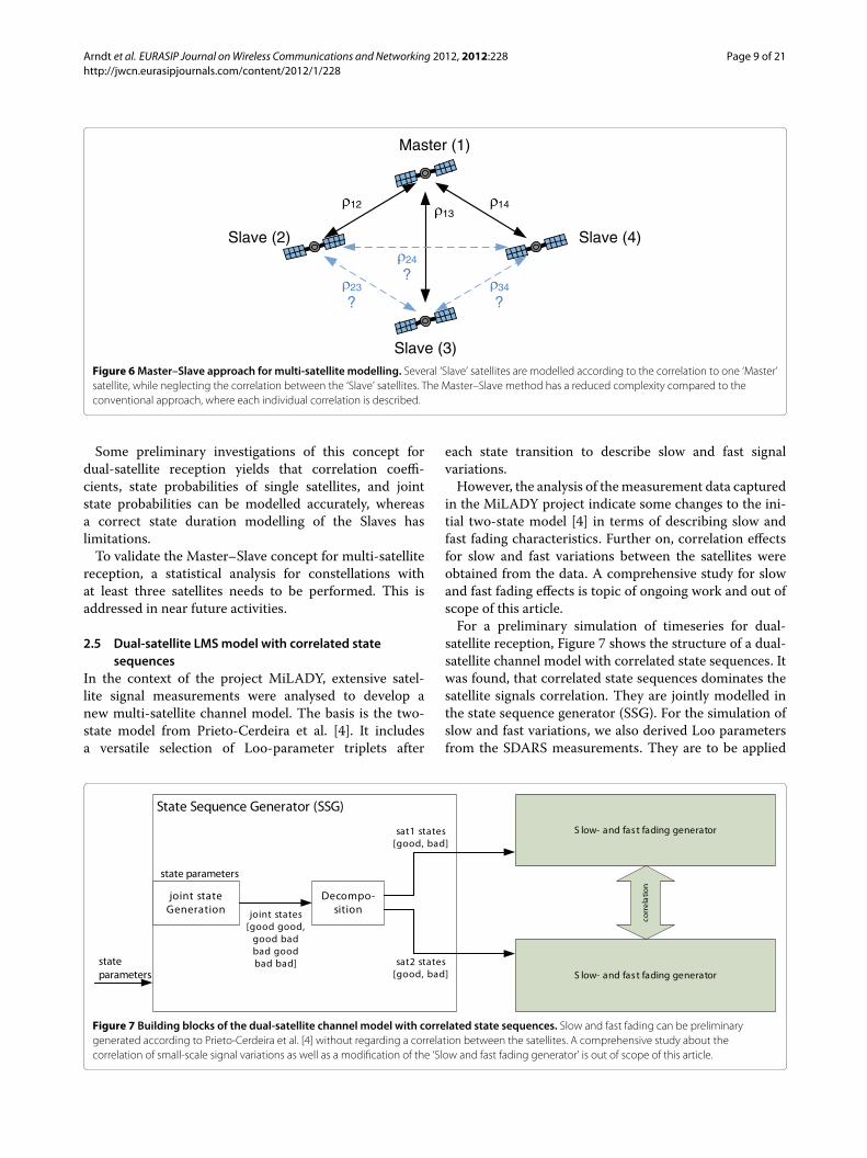
2.4 Channel state models for multi-satellite systemsIn general, all state models mentioned in the previoussubsections are extendable to multiple satellites. However,the number of required parameters for the models growsexponentially with the number of satellites. To avoidexcessive complexity for the state modelling with morethan two satellites, a ‘Master–Slave’ approach is planned[11]. Within the Master–Slave approach it is assumedthat each ‘Slave’ satellite depends only on a ‘Master’ satel-lite, whereas the correlation between the slaves is notdescribed (cf. Figure 6).

Table 3 Performance comparison of dual-satellite statemodels

Algorithm State probability State duration Modelmodelling modelling complexity

1st orderMarkov (Lutz)

perfect bad low

DynamicMarkov

perfect perfect high

Partial dynamicMarkov

bad perfect high

Semi-Markov,no fit

perfect perfect high

Semi-Markov,lognormal fit

good good medium

Semi-Markov,logn.fit+correction

perfect good medium

Semi-Markov,piecewise exp.fit

good good medium


Master (1)

Slave (2) Slave (4)

Slave (3)

1213

14

24

?34

?23

?

Figure 6Master–Slave approach for multi-satellite modelling. Several ‘Slave’ satellites are modelled according to the correlation to one ‘Master’satellite, while neglecting the correlation between the ‘Slave’ satellites. The Master–Slave method has a reduced complexity compared to theconventional approach, where each individual correlation is described.

Some preliminary investigations of this concept fordual-satellite reception yields that correlation coeffi-cients, state probabilities of single satellites, and jointstate probabilities can be modelled accurately, whereasa correct state duration modelling of the Slaves haslimitations.To validate the Master–Slave concept for multi-satellite

reception, a statistical analysis for constellations withat least three satellites needs to be performed. This isaddressed in near future activities.

2.5 Dual-satellite LMSmodel with correlated statesequences

In the context of the project MiLADY, extensive satel-lite signal measurements were analysed to develop anew multi-satellite channel model. The basis is the two-state model from Prieto-Cerdeira et al. [4]. It includesa versatile selection of Loo-parameter triplets after

each state transition to describe slow and fast signalvariations.However, the analysis of themeasurement data captured

in the MiLADY project indicate some changes to the ini-tial two-state model [4] in terms of describing slow andfast fading characteristics. Further on, correlation effectsfor slow and fast variations between the satellites wereobtained from the data. A comprehensive study for slowand fast fading effects is topic of ongoing work and out ofscope of this article.For a preliminary simulation of timeseries for dual-

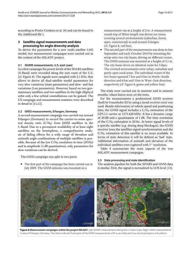
satellite reception, Figure 7 shows the structure of a dual-satellite channel model with correlated state sequences. Itwas found, that correlated state sequences dominates thesatellite signals correlation. They are jointly modelled inthe state sequence generator (SSG). For the simulation ofslow and fast variations, we also derived Loo parametersfrom the SDARS measurements. They are to be applied

Figure 7 Building blocks of the dual-satellite channel model with correlated state sequences. Slow and fast fading can be preliminarygenerated according to Prieto-Cerdeira et al. [4] without regarding a correlation between the satellites. A comprehensive study about thecorrelation of small-scale signal variations as well as a modification of the ‘Slow and fast fading generator’ is out of scope of this article.


according to Prieto-Cerdeira et al. [4] and can be found inthe Additional file 1.

3 Satellite signal measurements and dataprocessing for angle diversity analysis

To derive the parameters for a new multi-satellite LMSmodel, two measurement campaigns were carried out inthe context of the MiLADY project.

3.1 SDARSmeasurements, U.S. east coastIn a first campaign the power levels of the SDARS satellites(S-Band) were recorded along the east coast of the U.S.(cf. Figure 8). The signals were sampled with 2.1 kHz, thatallows to derive all dual-satellite model parameters forvery slow variations (state parameters) and slow- and fastvariations (Loo parameters). However, based on two geo-stationary satellites and two satellites in the high ellipticalorbit only a few orbital constellations can be gained. TheUS campaign and measurement statistics were describedin detail in [11,12].

3.2 GNSSmeasurements, Erlangen, GermanyA second measurement campaign was carried out aroundErlangen (Germany) to record the carrier-to-noise spec-tral density ratio (C/N0) from GNSS satellites in theL-Band. Due to a permanent availability of at least eightsatellites on the hemisphere, a comprehensive analy-sis of fading effects for a wide range of elevation andazimuth angle combinations of multiple satellites is pos-sible. Because of the low C/N0 resolution in time (20Hz)and in amplitude (1 dB quantisation), only parameters forslow variations can be derived.

The GNSS campaign was split in two parts:

• The first part of the campaign has been carried out inJuly 2009. The GNSS antenna was mounted on a

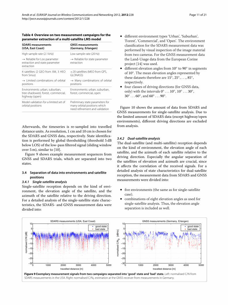
measurement van at a height of 2m. A measurementround-trip of 38 km length was driven ten times,covering several environments (suburban, forest,open, commercial) in and around Erlangen(cf. Figure 8, red line).

• The second part of the measurements was done in lateSeptember and early October 2010 by mounting thesetup onto two city buses, driving on different routes.The GNSS antenna was mounted at a height of 3.1m.The city buses drove an identical route for 3 days.The covered environments were urban, suburban andpartly open rural areas. The individual routes of thetwo buses spanned 7 km and 6 km in North–Southdirection and 6 km and 5 km in West–East direction,respectively (cf. Figure 8, green and yellow line).

The trials were carried out in summer and in autumnmonths, where leaves were on the trees.For the measurements a professional GNSS receiver

(built by Fraunhofer IIS by using a Javad receiver core) wasused. Beside information of vehicle speed and positioningdata, the GNSS signal includes a C/N0 estimation of theGPS L1 carrier at 1575.420MHz. It has a dynamic rangeof 20 dB and a quantisation of 1 dB. The time resolutionof the C/N0 estimation is 20Hz. At lower signal levels ofa specific satellite (e.g. during deep blockages), the GNSSreceiver loses the satellites signal synchronisation and theC/N0 estimation of this satellite is no more available. Interms of state detection it will be defined as ‘bad’ state.Additional information of azimuth and elevation of theindividual satellites were captured with 1◦ resolution.Table 4 summarises the main aspects of the two

MiLADY measurement campaigns.

3.3 Data processing and state identificationThe analysis pipeline for both the SDARS and GNSS datais similar. First, the signal is normalised to LOS level [13].

Figure 8Measurement campaigns within the project MiLADY. Left: SDARS measurements along the U.S. East Coast. Right: GNSS measurementsin area of Erlangen, Germany. The colors indicate three parts of the GNSS measurements with a van (red), and two city buses (green and yellow).


Table 4 Overview on twomeasurement campaigns for theparameter extraction of amulti-satellite LMSmodel

SDARSmeasurements(USA, East Coast)

GNSSmeasurements(Germany, Erlangen)

High sample rate (2.1 kHz) Low sample rate (20 Hz)

→ Reliable for Loo parameterextraction and state parameterextraction

→ Reliable for state parameterextraction

4 satellites (2 GEO from XM, 3 HEOfrom Sirius)

>20 satellites (MEO from GPS,GLONASS)

→ Limited combinations of orbitalpositions

→ Many combinations of orbitalpositions

Environments: urban, suburban,tree-shadowed, forest, commercial,highway (open)

Environments: urban, suburban,forest, commercial, open

Model validation for a limited set oforbital positions

Preliminary state parameters formany orbital positions whichneed refinement and validation

Afterwards, the timeseries is re-sampled into travelleddistance units. As resolution, 1 cm and 10 cm is chosen forthe SDARS and GNSS data, respectively. State identifica-tion is performed by global thresholding (threshold 5 dBbelow LOS) of the low-pass filtered signal (sliding windowover 5m), similar to [10].Figure 9 shows example measurement sequences from

GNSS and SDARS trials, which are separated into twostates.

3.4 Separation of data into environments and satellitepositions

3.4.1 Single-satellite analysisSingle-satellite reception depends on the kind of envi-ronment, the elevation angle of the satellite, and theazimuth of the satellite relative to the driving direction.For a detailed analysis of the single-satellite state charac-teristics, the SDARS- and GNSS measurement data weredivided into:

• different environment types ‘Urban’, ‘Suburban’,‘Forest’, ‘Commercial’, and ‘Open’. The environmentclassification for the SDARS measurement data wasperformed by visual inspection of the image materialfrom two cameras. For the GNSS measurement datathe Land-Usage data from the European Corineproject [14] was used.

• different elevation angles from 10◦ to 90◦ in segmentsof 10◦. The mean elevation angles represented bythese datasets therefore are 15◦, 25◦, . . ., 85◦,respectively.

• four classes of driving directions (for GNSS data,only) with the intervals 0◦ . . . 10◦, 10◦ . . . 30◦,30◦ . . . 60◦, and 60◦ . . . 90◦.

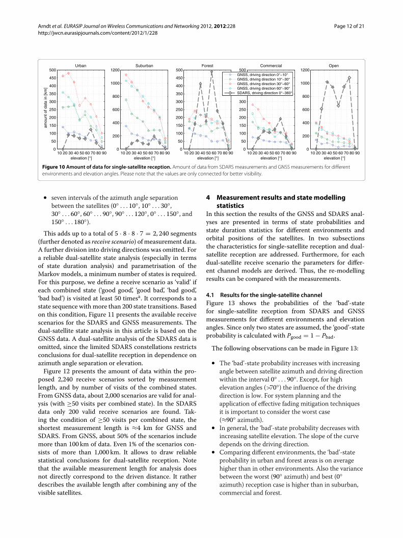
Figure 10 shows the amount of data from SDARS andGNSS measurements for single-satellite analysis. Due tothe limited amount of SDARS data (except highway/openenvironments), different driving directions are excludedfrom analysis.

3.4.2 Dual-satellite analysisThe dual-satellite (and multi-satellite) reception dependson the kind of environment, the elevation angle of eachsatellite, and the azimuth of each satellite relative to thedriving direction. Especially the angular separation ofthe satellites of elevation and azimuth are crucial, sinceit affects the correlation of the received signals. For adetailed analysis of state characteristics for dual-satellitereception, the measurement data from SDARS and GNSSmeasurements were divided into:

• five environments (the same as for single-satellitecase).

• combinations of eight elevation angles as used forsingle-satellite analysis. Thus, the elevation angleseparation is included as well.

0 1000 2000 3000 4000 5000−30

−25

−20

−15

−10

−5

0

5

10


norm

alis

ed C

/N0

[dB

Hz]

GNSS measurements (Germany, Erlangen)

good statebad state

0 1000 2000 3000 4000 5000−30

−25

−20

−15

−10

−5

0

5

10


norm

alis

ed C

/N [d

B]

SDARS measurements (USA, East Coast)

good statebad state

Figure 9 Exemplary measurement signals from two campaigns separated into ‘good’ state and ‘bad’ state. Left: normalised C/N fromSDARS measurements in the USA. Right: normalised C/N0 estimation at the GNSS receiver from measurements in Germany.


10 20 30 40 50 60 70 80 900

50

100

150

200

250

300

350

400

450

500

elevation [°]

Urban

amou

nt o

f dat

a in

[km

]

10 20 30 40 50 60 70 80 900

200

400

600

800

1000

1200

elevation [°]

Suburban

10 20 30 40 50 60 70 80 900

50

100

150

200

250

300

350

400

450

500

elevation [°]

Forest

10 20 30 40 50 60 70 80 900

50

100

150

200

250

300

350

400

450

500

elevation [°]

Commercial

10 20 30 40 50 60 70 80 900

200

400

600

800

1000

1200

elevation [°]

Open

Figure 10 Amount of data for single-satellite reception. Amount of data from SDARS measurements and GNSS measurements for differentenvironments and elevation angles. Please note that the values are only connected for better visibility.

• seven intervals of the azimuth angle separationbetween the satellites (0◦ . . . 10◦, 10◦ . . . 30◦,30◦ . . . 60◦, 60◦ . . . 90◦, 90◦ . . . 120◦, 0◦ . . . 150◦, and150◦ . . . 180◦).

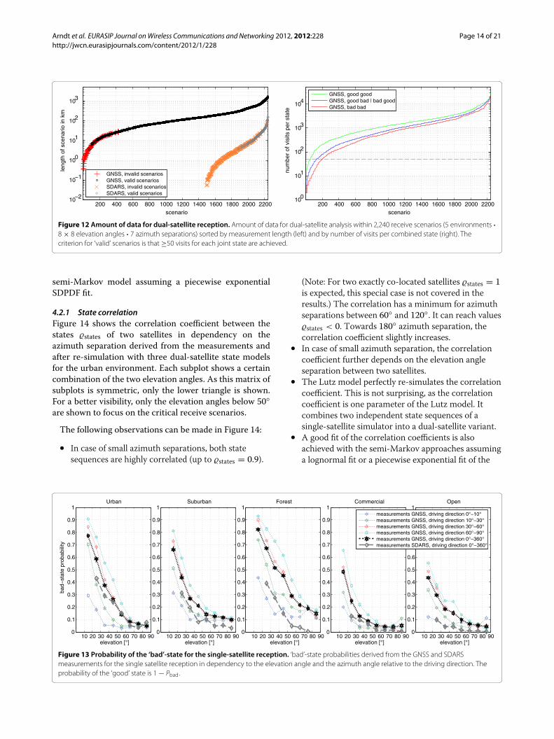
This adds up to a total of 5 · 8 · 8 · 7 = 2, 240 segments(further denoted as receive scenario) of measurement data.A further division into driving directions was omitted. Fora reliable dual-satellite state analysis (especially in termsof state duration analysis) and parametrisation of theMarkov models, a minimum number of states is required.For this purpose, we define a receive scenario as ‘valid’ ifeach combined state (‘good good’, ‘good bad’, ‘bad good’,‘bad bad’) is visited at least 50 timesa. It corresponds to astate sequence withmore than 200 state transitions. Basedon this condition, Figure 11 presents the available receivescenarios for the SDARS and GNSS measurements. Thedual-satellite state analysis in this article is based on theGNSS data. A dual-satellite analysis of the SDARS data isomitted, since the limited SDARS constellations restrictsconclusions for dual-satellite reception in dependence onazimuth angle separation or elevation.Figure 12 presents the amount of data within the pro-

posed 2,240 receive scenarios sorted by measurementlength, and by number of visits of the combined states.From GNSS data, about 2,000 scenarios are valid for anal-ysis (with ≥50 visits per combined state). In the SDARSdata only 200 valid receive scenarios are found. Tak-ing the condition of ≥50 visits per combined state, theshortest measurement length is ≈4 km for GNSS andSDARS. From GNSS, about 50% of the scenarios includemore than 100 km of data. Even 1% of the scenarios con-sists of more than 1,000 km. It allows to draw reliablestatistical conclusions for dual-satellite reception. Notethat the available measurement length for analysis doesnot directly correspond to the driven distance. It ratherdescribes the available length after combining any of thevisible satellites.

4 Measurement results and state modellingstatistics

In this section the results of the GNSS and SDARS anal-yses are presented in terms of state probabilities andstate duration statistics for different environments andorbital positions of the satellites. In two subsectionsthe characteristics for single-satellite reception and dual-satellite reception are addressed. Furthermore, for eachdual-satellite receive scenario the parameters for differ-ent channel models are derived. Thus, the re-modellingresults can be compared with the measurements.

4.1 Results for the single-satellite channelFigure 13 shows the probabilities of the ‘bad’-statefor single-satellite reception from SDARS and GNSSmeasurements for different environments and elevationangles. Since only two states are assumed, the ‘good’-stateprobability is calculated with Pgood = 1 − Pbad.

The following observations can be made in Figure 13:

• The ‘bad’-state probability increases with increasingangle between satellite azimuth and driving directionwithin the interval 0◦ . . . 90◦. Except, for highelevation angles (>70◦) the influence of the drivingdirection is low. For system planning and theapplication of effective fading mitigation techniquesit is important to consider the worst case(≈90◦ azimuth).

• In general, the ‘bad’-state probability decreases withincreasing satellite elevation. The slope of the curvedepends on the driving direction.

• Comparing different environments, the ‘bad’-stateprobability in urban and forest areas is on averagehigher than in other environments. Also the variancebetween the worst (90◦ azimuth) and best (0◦azimuth) reception case is higher than in suburban,commercial and forest.


ΔAz.=0°...10°

Urb

anel

evat

ion

2 [°

]

10

30

50

70

90ΔAz.=10°...30° ΔAz.=30°...60° ΔAz.=60°...90° ΔAz.=90°...120° ΔAz.=120°...150° ΔAz.=150°...180°

Sub

urba

nel

evat

ion

2 [°

]

10

30

50

70

90

For

est

elev

atio

n 2

[°]

10

30

50

70

90

Com

mer

cial

elev

atio

n 2

[°]

10

30

50

70

90

Ope

nel

evat

ion

2 [°

]

elevation 1 [°]10 30 50 70 90

10

30

50

70

90

elevation 1 [°]10 30 50 70 90

elevation 1 [°]10 30 50 70 90

elevation 1 [°]10 30 50 70 90

elevation 1 [°]10 30 50 70 90

elevation 1 [°]10 30 50 70 90

elevation 1 [°]10 30 50 70 90

amount of measurement data [km]

invalid 1 1.5 2.4 3.7 5.6 8.7 13.3 20.5 31.6 48.7 75.0 115.5 177.8 273.8 421.7 649.4 1000

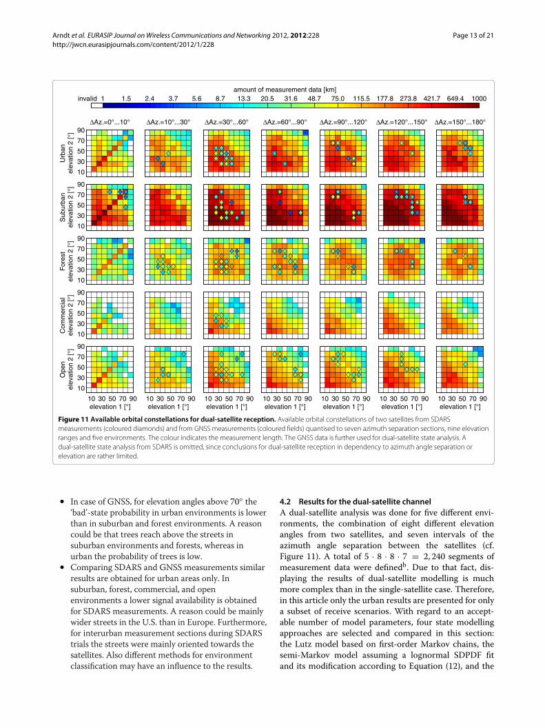
Figure 11 Available orbital constellations for dual-satellite reception. Available orbital constellations of two satellites from SDARSmeasurements (coloured diamonds) and from GNSS measurements (coloured fields) quantised to seven azimuth separation sections, nine elevationranges and five environments. The colour indicates the measurement length. The GNSS data is further used for dual-satellite state analysis. Adual-satellite state analysis from SDARS is omitted, since conclusions for dual-satellite reception in dependency to azimuth angle separation orelevation are rather limited.

• In case of GNSS, for elevation angles above 70◦ the‘bad’-state probability in urban environments is lowerthan in suburban and forest environments. A reasoncould be that trees reach above the streets insuburban environments and forests, whereas inurban the probability of trees is low.

• Comparing SDARS and GNSS measurements similarresults are obtained for urban areas only. Insuburban, forest, commercial, and openenvironments a lower signal availability is obtainedfor SDARS measurements. A reason could be mainlywider streets in the U.S. than in Europe. Furthermore,for interurban measurement sections during SDARStrials the streets were mainly oriented towards thesatellites. Also different methods for environmentclassification may have an influence to the results.

4.2 Results for the dual-satellite channelA dual-satellite analysis was done for five different envi-ronments, the combination of eight different elevationangles from two satellites, and seven intervals of theazimuth angle separation between the satellites (cf.Figure 11). A total of 5 · 8 · 8 · 7 = 2, 240 segments ofmeasurement data were definedb. Due to that fact, dis-playing the results of dual-satellite modelling is muchmore complex than in the single-satellite case. Therefore,in this article only the urban results are presented for onlya subset of receive scenarios. With regard to an accept-able number of model parameters, four state modellingapproaches are selected and compared in this section:the Lutz model based on first-order Markov chains, thesemi-Markov model assuming a lognormal SDPDF fitand its modification according to Equation (12), and the


200 400 600 800 1000 1200 1400 1600 1800 2000 2200100

101

102

103

104

scenario

num

ber

of v

isits

per

sta

te

200 400 600 800 1000 1200 1400 1600 1800 2000 220010−2

10−1

100

101

102

103

scenario

leng

th o

f sce

nario

in k

m

Figure 12 Amount of data for dual-satellite reception. Amount of data for dual-satellite analysis within 2,240 receive scenarios (5 environments ·8 × 8 elevation angles · 7 azimuth separations) sorted by measurement length (left) and by number of visits per combined state (right). Thecriterion for ‘valid’ scenarios is that ≥50 visits for each joint state are achieved.

semi-Markov model assuming a piecewise exponentialSDPDF fit.

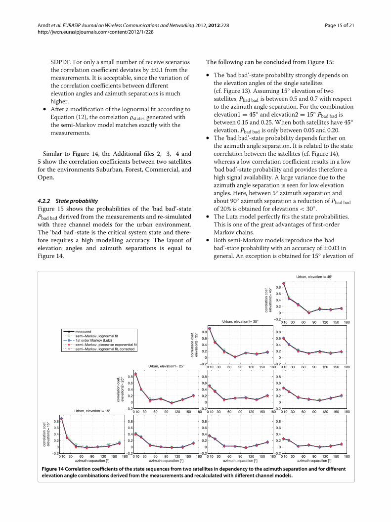
4.2.1 State correlationFigure 14 shows the correlation coefficient between thestates �states of two satellites in dependency on theazimuth separation derived from the measurements andafter re-simulation with three dual-satellite state modelsfor the urban environment. Each subplot shows a certaincombination of the two elevation angles. As this matrix ofsubplots is symmetric, only the lower triangle is shown.For a better visibility, only the elevation angles below 50◦are shown to focus on the critical receive scenarios.

The following observations can be made in Figure 14:

• In case of small azimuth separations, both statesequences are highly correlated (up to �states = 0.9).

(Note: For two exactly co-located satellites �states = 1is expected, this special case is not covered in theresults.) The correlation has a minimum for azimuthseparations between 60◦ and 120◦. It can reach values�states < 0. Towards 180◦ azimuth separation, thecorrelation coefficient slightly increases.

• In case of small azimuth separation, the correlationcoefficient further depends on the elevation angleseparation between two satellites.

• The Lutz model perfectly re-simulates the correlationcoefficient. This is not surprising, as the correlationcoefficient is one parameter of the Lutz model. Itcombines two independent state sequences of asingle-satellite simulator into a dual-satellite variant.

• A good fit of the correlation coefficients is alsoachieved with the semi-Markov approaches assuminga lognormal fit or a piecewise exponential fit of the

10 20 30 40 50 60 70 80 900

0.1

0.2

0.3

0.4

0.5

0.6

0.7

0.8

0.9

1

elevation [°]

Urban

bad−

stat

e pr

obab

ility

10 20 30 40 50 60 70 80 900

0.1

0.2

0.3

0.4

0.5

0.6

0.7

0.8

0.9

1

elevation [°]

Suburban

10 20 30 40 50 60 70 80 900

0.1

0.2

0.3

0.4

0.5

0.6

0.7

0.8

0.9

1

elevation [°]

Forest

10 20 30 40 50 60 70 80 900

0.1

0.2

0.3

0.4

0.5

0.6

0.7

0.8

0.9

1

elevation [°]

Commercial

10 20 30 40 50 60 70 80 900

0.1

0.2

0.3

0.4

0.5

0.6

0.7

0.8

0.9

1

elevation [°]

Open

Figure 13 Probability of the ‘bad’-state for the single-satellite reception. ‘bad’-state probabilities derived from the GNSS and SDARSmeasurements for the single satellite reception in dependency to the elevation angle and the azimuth angle relative to the driving direction. Theprobability of the ‘good’ state is 1 − Pbad.


SDPDF. For only a small number of receive scenariosthe correlation coefficient deviates by ±0.1 from themeasurements. It is acceptable, since the variation ofthe correlation coefficients between differentelevation angles and azimuth separations is muchhigher.

• After a modification of the lognormal fit according toEquation (12), the correlation �states generated withthe semi-Markov model matches exactly with themeasurements.

Similar to Figure 14, the Additional files 2, 3, 4 and5 show the correlation coefficients between two satellitesfor the environments Suburban, Forest, Commercial, andOpen.

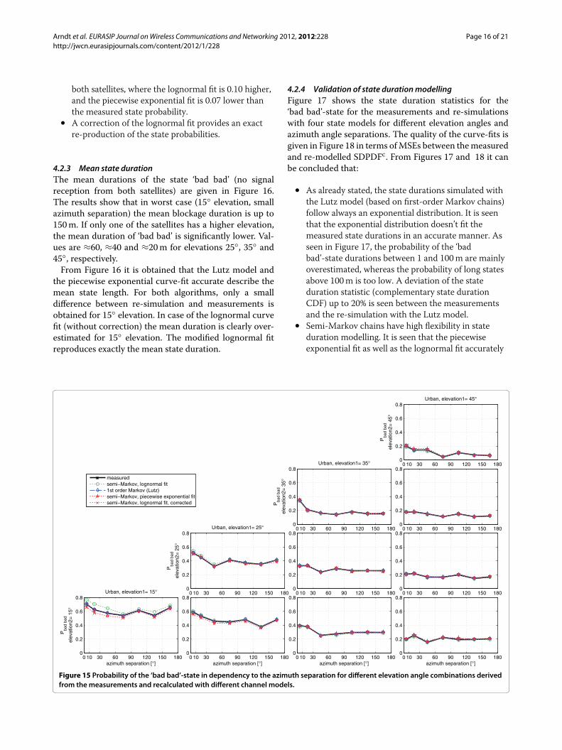
4.2.2 State probabilityFigure 15 shows the probabilities of the ‘bad bad’-statePbad bad derived from the measurements and re-simulatedwith three channel models for the urban environment.The ‘bad bad’-state is the critical system state and there-fore requires a high modelling accuracy. The layout ofelevation angles and azimuth separations is equal toFigure 14.

The following can be concluded from Figure 15:

• The ‘bad bad’-state probability strongly depends onthe elevation angles of the single satellites(cf. Figure 13). Assuming 15◦ elevation of twosatellites, Pbad bad is between 0.5 and 0.7 with respectto the azimuth angle separation. For the combinationelevation1 = 45◦ and elevation2 = 15◦ Pbad bad isbetween 0.15 and 0.25. When both satellites have 45◦elevation, Pbad bad is only between 0.05 and 0.20.

• The ‘bad bad’-state probability depends further onthe azimuth angle separation. It is related to the statecorrelation between the satellites (cf. Figure 14),whereas a low correlation coefficient results in a low‘bad bad’-state probability and provides therefore ahigh signal availability. A large variance due to theazimuth angle separation is seen for low elevationangles. Here, between 5◦ azimuth separation andabout 90◦ azimuth separation a reduction of Pbad badof 20% is obtained for elevations < 30◦.

• The Lutz model perfectly fits the state probabilities.This is one of the great advantages of first-orderMarkov chains.

• Both semi-Markov models reproduce the ‘badbad’-state probability with an accuracy of ±0.03 ingeneral. An exception is obtained for 15◦ elevation of

Figure 14 Correlation coefficients of the state sequences from two satellites in dependency to the azimuth separation and for differentelevation angle combinations derived from the measurements and recalculated with different channel models.


both satellites, where the lognormal fit is 0.10 higher,and the piecewise exponential fit is 0.07 lower thanthe measured state probability.

• A correction of the lognormal fit provides an exactre-production of the state probabilities.

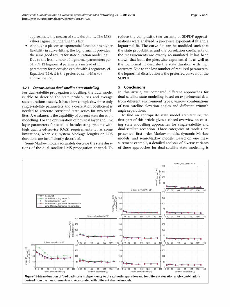
4.2.3 Mean state durationThe mean durations of the state ‘bad bad’ (no signalreception from both satellites) are given in Figure 16.The results show that in worst case (15◦ elevation, smallazimuth separation) the mean blockage duration is up to150m. If only one of the satellites has a higher elevation,the mean duration of ‘bad bad’ is significantly lower. Val-ues are ≈60, ≈40 and ≈20m for elevations 25◦, 35◦ and45◦, respectively.From Figure 16 it is obtained that the Lutz model and

the piecewise exponential curve-fit accurate describe themean state length. For both algorithms, only a smalldifference between re-simulation and measurements isobtained for 15◦ elevation. In case of the lognormal curvefit (without correction) the mean duration is clearly over-estimated for 15◦ elevation. The modified lognormal fitreproduces exactly the mean state duration.

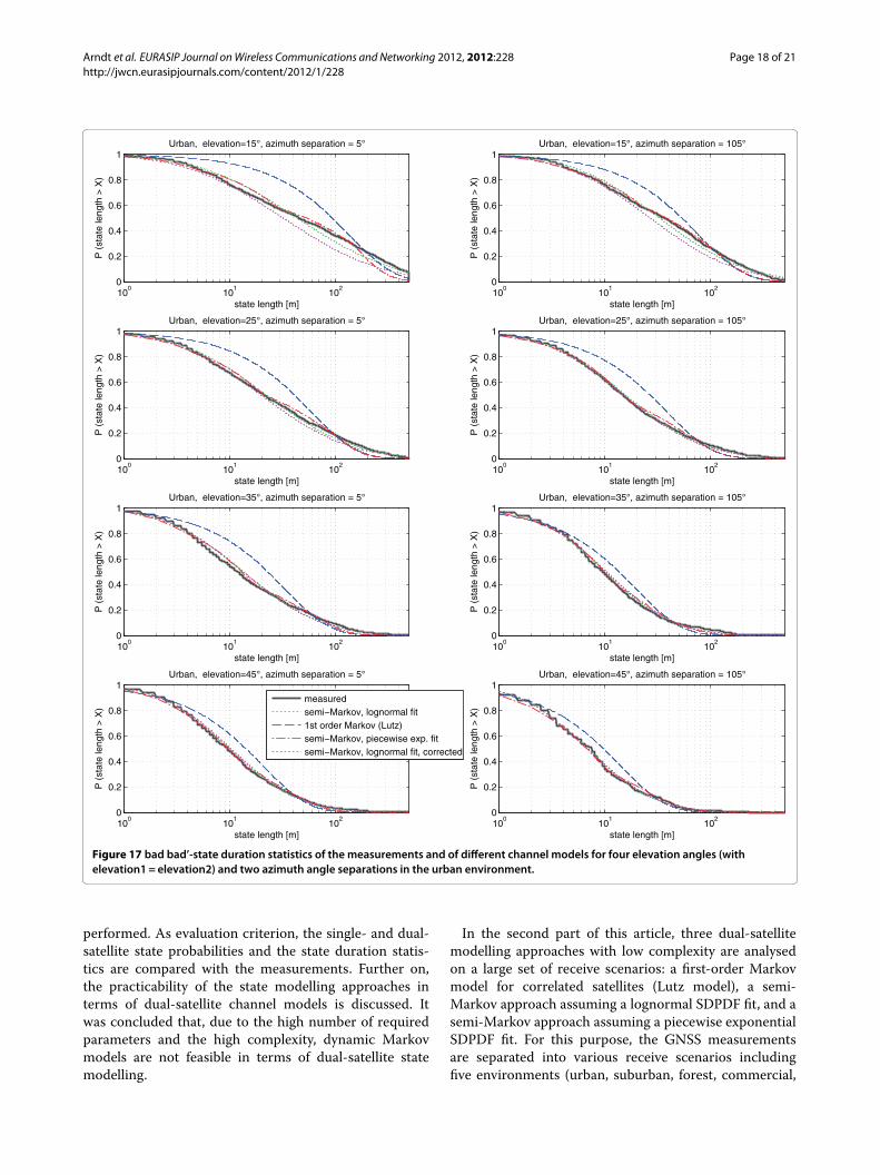
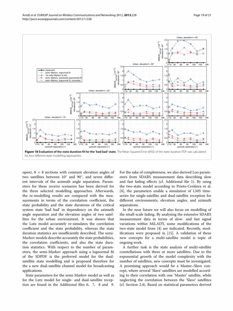
4.2.4 Validation of state durationmodellingFigure 17 shows the state duration statistics for the‘bad bad’-state for the measurements and re-simulationswith four state models for different elevation angles andazimuth angle separations. The quality of the curve-fits isgiven in Figure 18 in terms ofMSEs between themeasuredand re-modelled SDPDFc. From Figures 17 and 18 it canbe concluded that:

• As already stated, the state durations simulated withthe Lutz model (based on first-order Markov chains)follow always an exponential distribution. It is seenthat the exponential distribution doesn’t fit themeasured state durations in an accurate manner. Asseen in Figure 17, the probability of the ‘badbad’-state durations between 1 and 100m are mainlyoverestimated, whereas the probability of long statesabove 100m is too low. A deviation of the stateduration statistic (complementary state durationCDF) up to 20% is seen between the measurementsand the re-simulation with the Lutz model.

• Semi-Markov chains have high flexibility in stateduration modelling. It is seen that the piecewiseexponential fit as well as the lognormal fit accurately

Figure 15 Probability of the ‘bad bad’-state in dependency to the azimuth separation for different elevation angle combinations derivedfrom the measurements and recalculated with different channel models.


approximate the measured state durations. The MSEvalues Figure 18 underline this fact.

• Although a piecewise exponential function has higherflexibility in curve-fitting, the lognormal fit providesthe same good results for state duration modelling.Due to the less number of lognormal parameters perSDPDF (2 lognormal parameters instead of 11parameters for piecewise exp. fit with 4 segments, cf.Equation (11)), it is the preferred semi-Markovapproximation.

4.2.5 Conclusions on dual-satellite statemodellingFor dual-satellite propagation modelling, the Lutz modelis able to describe the state probabilities and averagestate durations exactly. It has a low complexity, since onlysingle-satellite parameters and a correlation coefficient isneeded to generate correlated state series for two satel-lites. A weakness is the capability of correct state durationmodelling. For the optimisation of physical layer and linklayer parameters for satellite broadcasting systems withhigh quality-of-service (QoS) requirements it has somelimitations, when e.g. system blockage lengths or LOSdurations are insufficiently described.Semi-Markovmodels accurately describe the state dura-

tions of the dual-satellite LMS propagation channel. To

reduce the complexity, two variants of SDPDF approxi-mations were analysed: a piecewise exponential fit and alognormal fit. The curve fits can be modified such thatthe state probabilities and the correlation coefficients ofthe measurements are exactly re-simulated. It has beenshown that both the piecewise exponential fit as well asthe lognormal fit describe the state duration with highaccuracy. Due to the low number of required parameters,the lognormal distribution is the preferred curve fit of theSDPDF.

5 ConclusionsIn this article, we compared different approaches fordual-satellite state modelling based on experimental datafrom different environment types, various combinationsof two satellite elevation angles and different azimuthangle separations.To find an appropriate state model architecture, the

first part of this article gives a closed overview on exist-ing state modelling approaches for single-satellite anddual-satellite reception. Three categories of models arepresented: first-order Markov models, dynamic Markovmodels, and semi-Markov models. Based on one mea-surement example, a detailed analysis of diverse variantsof these approaches for dual-satellite state modelling is

Figure 16Mean duration of ‘bad bad’-state in dependency to the azimuth separation and for different elevation angle combinationsderived from the measurements and recalculated with different channel models.


10 10 100

0.2

0.4

0.6

0.8

1

state length [m]

P (

stat

e le

ngth

> X

)

Urban, elevation=15°, azimuth separation = 5°

10 10 100

0.2

0.4

0.6

0.8

1

state length [m]


P (

stat

e le

ngth

> X

)10 10 100

0.2

0.4

0.6

0.8

1

state length [m]

P (

stat

e le

ngth

> X

)


10 10 100

0.2

0.4

0.6

0.8

1

state length [m]


P (

stat

e le

ngth

> X

)

10 10 100

0.2

0.4

0.6

0.8

1

state length [m]

P (

stat

e le

ngth

> X

)


10 10 100

0.2

0.4

0.6

0.8

1

state length [m]


P (

stat

e le

ngth

> X

)

10 10 100

0.2

0.4

0.6

0.8

1

state length [m]

P (

stat

e le

ngth

> X

)


measuredsemi−Markov, lognormal fit1st order Markov (Lutz)semi−Markov, piecewise exp. fitsemi−Markov, lognormal fit, corrected

10 10 100

0.2

0.4

0.6

0.8

1

state length [m]


P (

stat

e le

ngth

> X

)

Figure 17 bad bad’-state duration statistics of the measurements and of different channel models for four elevation angles (withelevation1= elevation2) and two azimuth angle separations in the urban environment.

performed. As evaluation criterion, the single- and dual-satellite state probabilities and the state duration statis-tics are compared with the measurements. Further on,the practicability of the state modelling approaches interms of dual-satellite channel models is discussed. Itwas concluded that, due to the high number of requiredparameters and the high complexity, dynamic Markovmodels are not feasible in terms of dual-satellite statemodelling.

In the second part of this article, three dual-satellitemodelling approaches with low complexity are analysedon a large set of receive scenarios: a first-order Markovmodel for correlated satellites (Lutz model), a semi-Markov approach assuming a lognormal SDPDF fit, and asemi-Markov approach assuming a piecewise exponentialSDPDF fit. For this purpose, the GNSS measurementsare separated into various receive scenarios includingfive environments (urban, suburban, forest, commercial,


Figure 18 Evaluation of the state duration fit for the ‘bad bad’-state. The Mean Squared Error (MSE) of the state duration PDF was calculatedfor four different state modelling approaches.

open), 8 × 8 sections with constant elevation angles oftwo satellites between 10◦ and 90◦, and seven differ-ent intervals of the azimuth angle separation. Param-eters for these receive scenarios has been derived forthe three selected modelling approaches. Afterwards,the re-modelling results are compared with the mea-surements in terms of the correlation coefficient, thestate probability and the state durations of the criticalsystem state ‘bad bad’ in dependency on the azimuthangle separation and the elevation angles of two satel-lites for the urban environment. It was shown thatthe Lutz model accurately re-simulates the correlationcoefficient and the state probability, whereas the stateduration statistics are insufficiently described. The semi-Markov models describe accurately the state probabilities,the correlation coefficients, and also the state dura-tion statistics. With respect to the number of param-eters, the semi-Markov approach using a lognormal fitof the SDPDF is the preferred model for the dual-satellite state modelling and is proposed therefore forthe a new dual-satellite channel model for broadcastingapplications.State parameters for the semi-Markov model as well as

for the Lutz model for single- and dual-satellite recep-tion are found in the Additional files 6, 7, 8 and 9.

For the sake of completeness, we also derived Loo param-eters from SDARS measurement data describing slowand fast fading effects (cf. Additional file 1). By usingthe two-state model according to Prieto-Cerdeira et al.[4], the parameters enable a simulation of LMS time-series for single-satellite and dual-satellite reception fordifferent environments, elevation angles, and azimuthseparations.In the near future we will also focus on modelling of

the small-scale fading. By analysing the extensive SDARSmeasurement data in terms of slow- and fast signalvariations within MiLADY, some modifications of thetwo-state model from [4] are indicated. Recently, mod-ifications were proposed in [15]. A validation of thesenew concepts for a multi-satellite model is topic ofongoing work.A further task is the state analysis of multi-satellite

constellations with three or more satellites. Due to theexponential growth of the model complexity with thenumber of satellites, new concepts must be investigated.A promising approach would be a Master–Slave con-cept, where several ‘Slave’ satellites are modelled accord-ing to their correlation with one ‘Master’ satellite, whileneglecting the correlation between the ‘Slave’ satellites(cf. Section 2.4). Based on statistical parameters derived


frommeasurement data (such as the joint state probabilityfor ‘bad bad bad’ for three satellites), the Master–Slaveconcept will be evaluated.To improve the consistency of a state parameter

database, activities are planned to extract state param-eters with alternative methods, such as the analysis ofenvironmental images from fish-eye cameras.

6 Endnotesa The state duration statistic of a combined state include≥ 50 elements.b For single-satellite analysis only 160 segments (8 eleva-tion angles, 5 environments and 4 driving directions) wererequired.c Note: The MSE is estimated between measured andre-simulated state duration PDF, but the figures showthe complementary CDF of the state duration for bettervisibility.

Additional files

Additional file 1: Two-state model parameters derived from SDARSmeasurements.

Additional file 2: Correlation coefficients of the state sequences fromtwo satellites in dependency on the azimuth separation and fordifferent elevation angle combinations derived from themeasurements and recalculated with different channel models in thesuburban environment.

Additional file 3: Correlation coefficients of the state sequences fromtwo satellites in dependency on the azimuth separation and fordifferent elevation angle combinations derived from themeasurements and recalculated with different channel models in theforest environment.

Additional file 4: Correlation coefficients of the state sequences fromtwo satellites in dependency on the azimuth separation and fordifferent elevation angle combinations derived from themeasurements and recalculated with different channel models in thecommercial environment.

Additional file 5: Correlation coefficients of the state sequences fromtwo satellites in dependency on the azimuth separation and fordifferent elevation angle combinations derived from themeasurements and recalculated with different channel models in theopen environment.

Additional file 6: State parameters from SDARSmeasurements for afirst-order Markov model and a semi-Markov model for thesingle-satellite reception. Each row corresponds to one receive scenario:environment, elevation, driving direction with resp. to satellite azimuth.

Additional file 7: State parameters from GNSSmeasurements for afirst-order Markov model and a semi-Markov model for thesingle-satellite reception. Each row corresponds to one receive scenario:environment, elevation, driving direction with resp. to satellite azimuth.

Additional file 8: List of parameters for the semi-Markov model usinga lognormal state duration PDF for dual-satellite state modelling.Each row corresponds to one receive scenario: environment, elevation ofsatellite 1, elevation of satellite 2, azimuth angle separation. 20 parametersper receive scenario are required: μ1, σ1, . . . , μ4, σ4 are the parameters todescribe the lognormal distribution of four joint states with the order‘good good’, ‘good bad’, ‘bad good’, ‘bad bad’ (cf. Equation (9)); theparameters pij (with i �= j and i, j ∈ 1, 2, 3, 4) are the state transitionprobabilities according to the joint state

transition probability matrixPtrans; the state transition probabilities pii arezero.

Additional file 9: List of parameters for the Lutz model fordual-satellite state modelling. Each row corresponds to one receivescenario: environment, elevation of satellite 1, elevation of satellite 2,azimuth angle separation. The parameters for one receive scenario are acorrelation coefficient and the state transition probabilities of two satellites(9 parameters).

Competing interestsThe authors declare that they have no competing interests.

AcknowledgementsThe GNSS and SDARS measurements were carried out in the context of theproject MiLADY. This project is funded by the ARTES 5.1 Programme of theTelecommunications and Integrated Applications Directorate of the EuropeanSpace Agency.

Author details1Ilmenau University of Technology, Ilmenau, Germany. 2Fraunhofer Institutefor Integrated Circuits IIS, Erlangen, Germany. 3European Space Agency,ESTEC, Noordwijk, The Netherlands.

Received: 29 November 2011 Accepted: 18 May 2012Published: 23 July 2012

References1. C Loo, in ICC ’84 - Links for the future: Science, systems and services for

communications, Proceedings of the International Conference onCommunications, vol. 2, A statistical model for a land mobile satellite link.(Amsterdam, The Netherlands, 1984), pp. 588–594

2. E Lutz, D Cygan, M Dippold, F Dolainsky, W Papke, The land mobilesatellite communication channel-Recording, statistics, and channelmodel, IEEE Trans. Veh. Technol. 40, 375–386 (1991)

3. F Perez-Fontan, M Vazquez-Castro, CE Cabado, JP Garcia, E Cubista,Statistical modeling of the LMS channel, IEEE Trans. Veh. Technol. 50(6),1549–1567 (2001)

4. R Prieto-Cerdeira, F Perez-Fontan, P Burzigotti, A Bolea-Alamanac, ISanchez-Lago, Versatile two-state land mobile satellite channel modelwith first application to DVB-SH analysis, Int. J. Satell. Commun. Netw. 28,291–315 (2010)

5. DVB BlueBook A120 (2008-05). DVB-SH Implementation Guidelines.http://www.dvb-h.org/technology.htm

6. PP Robet, BG Evans, A Ekman, Land mobile satellite communicationchannel model for simultaneous transmission from a land mobileterminal via two separate satellites, Int. J. Satell. Commun. 10(3), 139–154(1992). http://dx.doi.org/10.1002/sat.4600100304

7. E Lutz, A Markov model for correlated land mobile satellite channels, Int. J.Satell. Commun. 14, 333–339 (1996)

8. ITU-R P.681-6, Propagation Data Required for the Design of Earth SpaceLand Mobile Telecommunication Systems 2003

9. M Milojevic, M Haardt, E Eberlein, A Heuberger, Channel modeling formultiple satellite broadcasting systems, IEEE Trans. Broadcast. 55(4),705–718 (2009)

10. LE Braten, T Tjelta, Semi-Markov multistate modeling of the land mobilepropagation channel for geostationary satellites, IEEE Trans. AntennasPropag. 50(12), 1795–1802 (2002)

11. E Eberlein, A Heuberger, T Heyn, in ESAWorkshop on RadiowavePropagationModels, Tools and Data for Space Systems, Channel models forsystems with angle diversity—the MiLADY project, (Noordwijk, TheNetherlands, 2008)

12. D Arndt, A Ihlow, A Heuberger, T Heyn, E Eberlein, R Prieto-Cerdeira, inProceedings of the IEEE International Symposium on BroadbandMultimediaSystems and Broadcasting (BMSB),Mobile satellite broadcasting with anglediversity—performance evaluation based on measurements. (Shanghai,China, 2010), pp. 1–8

13. D Arndt, A Ihlow, A Heuberger, T Heyn, E Eberlein, in Proceedings of the10thWorkshop Digital Broadcasting, Land mobile satellite channelcharacteristics from the miLADY project. (Ilmenau, Germany, 2009), pp.49–55

http://www.biomedcentral.com/content/supplementary/1687-1499-2012-228-S1.xls

http://www.biomedcentral.com/content/supplementary/1687-1499-2012-228-S2.pdf








http://www.dvb-h.org/technology.htm

http://dx.doi.org/10.1002/sat.4600100304


14. Corine Land cover - Technical guide. Office for official publications of theEuropean Communities. Luxembourg. 1994

15. D Arndt, T Heyn, J Konig, A Ihlow, A Heuberger, R Prieto-Cerdeira, EEberlein, in Proceedings of the IEEE International Symposium on BroadbandMultimedia Systems and Broadcasting (BMSB), Extended two-statenarrowband LMS propagation model for S-band, (Seoul, South Korea,2012)

doi:10.1186/1687-1499-2012-228Cite this article as: Arndt et al.: State modelling of the land mobilepropagation channel for dual-satellite systems. EURASIP Journal on WirelessCommunications and Networking 2012 2012:228.

Submit your manuscript to a journal and benefi t from:

7 Convenient online submission

7 Rigorous peer review

7 Immediate publication on acceptance

7 Open access: articles freely available online

7 High visibility within the fi eld

7 Retaining the copyright to your article

Submit your next manuscript at 7 springeropen.com

RESEARCH OpenAccess …RESEARCH OpenAccess Statemodellingofthelandmobile...

Documents

Transcript of RESEARCH OpenAccess …RESEARCH OpenAccess Statemodellingofthelandmobile...