RESEARCH ON LONGITUDINAL CONTROL ALGORITHM FOR FLYING WING UAV BASED ON LQR...

INTERNATIONAL JOURNAL ON SMART SENSING AND INTELLIGENT SYSTEMS VOL. 6, NO. 5, DECEMBER 2013

2155

RESEARCH ON LONGITUDINAL CONTROL ALGORITHM

FOR FLYING WING UAV BASED ON LQR TECHNOLOGY

Yibo LI1*, Chao Chen1, Wei Chen2 1College of automation Shen Yang Aerospace University, Shenyang 110136 Liaoning, China

2AVIC Cheng Du aircraft industrial (group) Co., Ltd. Chengdu 610000, China

Emails: [email protected], [email protected], [email protected]

*Correspondent author: Yibo LI, [email protected]

Submitted: June.30, 2013 Accepted: Nov.23, 2013 Published: Dec.16, 2013

Abstract- Linear Quadratic Regulator (LQR) is widely used in many practical engineering fields due to

good stability margin and strong robustness. But there is little literature reports the technology that has

been used to control the flying wing unmanned aerial vehicles (UAV). In this paper, aiming at the

longitudinal static and dynamic characteristics of the flying wing UAV, LQR technology will be

introduced to the flying wing UAV flight control. The longitudinal stability augmentation control law

and longitudinal attitude control law are designed. The stability augmentation control law is designed

by using output feedback linear quadratic method. It can not only increase the longitudinal static

stability, but also improve the dynamic characteristics. The longitudinal attitude control law of the

flying wing UAV is designed by using command tracking augmented LQR method. The controller can

realize the control and maintain the flight attitude and velocity under the condition without breaking

robustness of LQR. It solves the command tracking problems that conventional LQR beyond reach.

Yibo LI, Chao Chen, Wei Chen. RESEARCH ON LONGITUDINAL CONTROL ALGORITHM FOR FLYING WING UAV BASED ON LQR TECHNOLOGY

2156

Considering that some state variables of the system are difficult to obtain directly, a control method that

called quasi-command tracking augmented LQR is designed by combing with the reduced order

observer, it retains all the features of command tracking augmented LQR and more suitable for the

application of practice engineering. Finally, the control laws are simulated under the environment of

Matlab/Simulink. The results show that the longitudinal control laws of the flying wing UAV which are

designed based on LQR can make the flying wing UAV achieve satisfactory longitudinal flying quality.

Index terms: Flying wing UAV, UAV modeling, augmented LQR method, longitudinal stability augmentation,

longitudinal attitude control, dimension reduction observer.

I. INTRODUCTION

Because flying wing UAV adopts the technology of wing-fuselage blending, horizontal tail and

vertical tail of the conventional configuration are canceled, the plane looks like a lifting surface.

It not only improves the lift-to-drag ratio, reduces the Radar Cross Section, but also enlarges the

range of flight envelope and cuts down on energy consumption [1][2]. But this exclusive

pneumatic layout has brought many problems to the design of flight control system. On the one

hand, because of the aspect ratio of the flying wing UAV is large and the fuselage is short, there

is no tail plane or horizontal tail, which results in the decrease of the longitudinal static stability

and the control effectiveness. On the other hand, the vertical tail of the aircraft is canceled made

the transverse lateral damping of aircraft declined, meanwhile we need to add new control

mechanism to achieve the yaw of plane. Undoubtedly these will increase the difficulty in

designing the flight control law [3][4].

In the method of multivariable feedback control system design, the LQR technology is widely

used in many practical engineering fields [5-11], especially in the control of conventional layout

fixed-wing UAV and unmanned helicopter [12-16], which has many advantages such as more

than 60°phase margin, infinite amplitude margin and strong robustness. In literature [12][13], it

has realized the stability augmentation control of conventional layout fixed-wing UAV by using

conventional LQR method. It has effectively solved the problems that UAV is disturbed by air

current easily and has poor flight stability. The shortage is that there are large numbers of


2157

feedback gain to seek, and it is not convenient for the application of practical engineering. The

explicit and implicit model following technology, based on linear quadratic regulator theory, are

respectively applied to design unmanned helicopter and fixed-wing UAV autopilot in literature

[14][15], although the method has achieved the attitude control and hold of UAV, it needs the

high-precision reference model, and the controller structure is also more complicated. Literature

[16] presents a combined control method based on active modeling and traditional LQG control

theory，which can be effectively adapted to model uncertainty and applied to flight control of

unmanned helicopter, the result shows that the method can ensure the flight stability of the

unmanned helicopter in uncertain wind environment, however the shortage is that LQG control

increases the complexity of the control system owing to estimate of the whole state variables, but

it needn’t in practical engineering.

At present, the design of flight control law of flying wing UAV mainly adopts classic control

theory such as the root locus method and frequency domain analysis method[17]. Although the

method is reliable and intuitive, there will be heavy workload by using classic control methods to

design feedback loop, and sometimes it’s difficult to satisfy the design requirements for complex

flight control system with multiple inputs multiple outputs and strong coupling. LQR technology

with its strong robustness has been successfully and widely used in the fields of the fixed-wing

UAV, unmanned helicopter and other engineering. But there are no reports on the flight control

of the flying wing UAV. Therefore, the LQR technology with its good robustness will be

introduced into the flying wing UAV flight control in this paper, and the longitudinal stability

augmentation control law and longitudinal attitude control law of the flying wing UAV will be

designed respectively. The design of stability augmentation control law is accomplished by using

output feedback linear quadratic method. It can not only increase the longitudinal static stability,

but also improve the dynamic characteristics. Meanwhile, the numbers of feedback gain have

been reduced compared with the conventional LQR state regulator. It is convenient for the

applications of practical engineering. A special control system augmented method and

conventional LQR method are combined together to obtain a command tracking augmented LQR

method that can used control the attitude of the flying wing UAV. The controller has strong

robustness and simple structure, it realizes tracking control with zero static error of the flight

velocity and pitch angle, thus it solves the command tracking problems that conventional LQR

regulator beyond reach. Considering that some state variables of the system are difficult to obtain


2158

directly (e.g. angle of attack), a control method that called quasi-command tracking augmented

LQR is designed by combing with the reduced order observer, it retains all the features of

command tracking augmented LQR method and more suitable for the application of practical

engineering.

Finally, the longitudinal model of the flying wing UAV will be established and the control

method will be simulated under the environment of Matlab/Simulink. The results show that the

longitudinal control laws for the flying wing UAV based on LQR can make the flying wing UAV

achieve satisfactory longitudinal flying qualities.

II. LONGITUDINAL MODELING OF THE FLYING WING UAV

a. Control surfaces of the flying wing UAV

Flying wing UAV has no horizontal stabilizer and vertical tail, so control mechanism of the

aircraft can only be installed on the trailing edge of the wing as shown in figure 1.

Figure 1. The high-altitude long-endurance flying wing UAV

There is a pair of elevators in the inner side of the trailing edge of the UAV, which is used to

control pitch and lift of the plane. The laterals of elevator are provided with symmetrical elevons,

which are used for lift enhancement and rolling motion; A new kind of control mechanism named

split-drag-rudder is adopted to control the lateral motion of the UAV. Two split-drag-rudders are

on the tail edge near the tip wing, which are far from the symmetry plane. When the split-drag-

rudder open up a certain angle in one side, the drag-force will be increased on the same side and

get an unbalanced yawing moment, which lead the UAV yawing to the same side. While when

the two split-drag-rudders are opened up on both two sides, the drag force will be increased


2159

noticeably. So the split-drag-rudder can be used to the velocity control of the UAV, such as in

approaching and landing, air refueling and etc. Due to the split-drag-rudders are mounted on the

tail edge near the tip wing, the distance between the control mechanism and gravity of the UAV

is far, the effects on longitudinal pitching motion of the UAV by drag rudder can’t be ignored, so

it should be taken into consideration while modeling.

b. Longitudinal motion equation of the flying wing UAV

Considering the UAV motion is a very complex dynamic process, it is a nonlinear time-varying

system in the flight process, the whole movement is influenced by various factors. For example,

earth curvature, atmospheric motion, elastic deformation of the plane, acceleration of gravity and

so on. It will be very complex to take various factors into account, which makes the modeling

hardly realized. Therefore, we need to make the following assumptions of the flying wing UAV

motion system in the modeling process [18][19].

(1) The UAV is rigid and the quality is constant.

(2) The earth fixed axis is regarded as an inertial coordinate system

(3) The acceleration of gravity g is a constant;

(4) The plane XOZ of the body coordinate system of the flying wing UAV is symmetric, not only

the geometry appearance of the UAV is symmetric, but also the internal quality distribution.

xT

t

L

aM

G

D

v

Figure 2. Force analysis of the flying wing UAV longitudinal motion

The longitudinal dynamics and the kinematics model of the flying wing UAV are built based on

the above assumptions. Longitudinal stress analysis to the UAV (select a state to climbing

process of the UAV) is shown as in Figure 2. Longitudinal motion equation of the flying wing

UAV can be described as:


2160

cos( ) sin

sin( ) cost

t

z z

mv T D mg

mv T L mg

I M

(1)

Where m is the quality of the UAV, life force L and drag force D are aerodynamic forces of the

UAV, and pitching moment Mz is aerodynamic moment, T is the thrust of the UAV, φt is the

intersection angle between the thrust T and the body axis x, Iz is the yaw moment of the inertia,

is the path angle of the UAV. Aerodynamic force and aerodynamic moments are nonlinear

function about the speed v, the atmosphere density of the height of flight, pitch rate q , angle of

attack and the rudder deflection angle. The nonlinear functions are expressed according to the

aerodynamic principle as follows :

2 20

2 20

2 20

1 1( )

2 21 1

( )2 2

1 1( )

2 2 2

e d

e

e d

vd D D D D e D d

v qL L L L L L e

v qz M M M M M M e M d

D V SC V S C C C V C C

L V SC V S C C C V C q C

cM V ScC V Sc C C C V C q C C

V

(2)

where S is the wing reference area, c is the wing mean geometric chord, 0DC , DC , vDC etc are the

aerodynamic derivatives of the UAV, δe is the elevator angle, δd is the split drag rudder angle.

Thrust T of the UAV is a nonlinear function about the atmosphere density, the flight velocity and

throttle opening. The expression is:

( , , )tT T v (3)

where δt is the throttle opening. Substitute above formula (2) (3) into formula (1), we can get

complete longitudinal mathematical model of the flying wing UAV. Since the model consists of

nonlinear differential equations, it is not convenient to analysis the system and design the control

law. Therefore, we select a typical flight status to linear processing, which is based on the

disturbance theory and the coefficient freezing method, the differential equations with constant

coefficients of the system are:


2161

1 1 11 1 1

2 22 2 2

3 3 3 3 3

5 5 5

0 0

01 0

0 0 0

0 0 1 0 0 0 0 00 0 0 0 0

e t d

e t

e d

v

v e

v q t

d

v

n n nn n nv v

n nn n n

n n nq q n n

n n nh h

(4)

Where m

DTn vtv

v

)cos( 01

, m

DTgn t

)cos(

cos 0001 , 01 cos gn , m

Dn e

e

1 ,

m

Dn d

d

1 , m

Tn tt

t

)cos( 01

, 0

02

)sin(

mv

LTn vtv

v

, 0

2 mv

Ln e

e

0

00

0

02

)sin(sin

mv

LTgn t

, 0

02

sin

v

gn

, y

ee I

Mn

3

0

02

)sin(

mv

Tn tt

t

, y

vv I

Mn 3

, yI

Mn

3

, y

qq I

Mn 3

, y

dd I

Mn

3

5 0sinvn , 5 0 0cosn v , 5 0 0cosn v .

The 0 0 0 0, , ,v T are known as parameters of typical flight status, longitudinal modeling of the

UAV is completed.

III. THE FLYING WING UAV LONGITUDINAL STABILITY

AUGMENTATION CONTRAL

As the fuselage of the flying wing UAV is short, it results in the control effectiveness of elevator

and elevon on the tail edge of the UAV low. In order to improve the maneuverability, the static

stability can be properly relaxed. The aerodynamic center will shift backward, which may

weaken the UAV’s longitudinal static stability when the UAV flying at transonic or at high angle

of attack. As a compromise between the longitudinal stability and maneuverability, the aircraft's

center of gravity can be configured at the position between the aerodynamic center at high angle

of attack and high-speed and the aerodynamic center at low-speed and low angle of attack.

Therefore, the static stability can be maintained at low speed and low angle of attack, and the

instability at high speed and high angle of attack is still acceptable. As a result, only at high-

speed and high angle of attack, longitudinal stability augmentation is needed.


2162

a. Output feedback linear quadratic regulator

Although the traditional linear quadratic regulator can achieve stability augmentation of the UAV,

it needs all the state variables information of the system and heavy workload, which is not

conducive to engineering practice. Therefore, there is output feedback linear quadratic method to

design the longitudinal stability augmentation control law of the flying wing UAV. Combined

with section Ⅱ.b, consider the following three rudder loop models:

Elevator: 20

20e euS

, throttle thrust: 20

20t tuS

, and split-drag-rudder: 40

20d duS

.

The longitudinal augmented state equation and output equation of the flying wing UAV are:

x Ax Bu

y Cx

(5)

Where Te t dx v q is the system state vector, Te t du u u u is the

control vector, and Ty v q is the output of the UAV. Choose form for output

feedback:

u Ky (6)

where K is the feedback gain matrix of the corresponding dimension. Substitute (6) into the above

formula (5), we obtain the following state equation of closed loop system:

( )x A BKC x A x (7)

The purpose of designing the stability augmentation control law is to adjust the UAV state, so

that any errors of the initial conditions can be preserved to zero, which can ensure the flight

stability. Thus we can minimize the following quadratic cost function by selecting the control

input u:

0

1( )

2T TJ x Qx u Ru dt

(8)

where, Q and R are the weighting matrices, Q is the semi-positive definite symmetric matrix and

R is the positive definite symmetric matrix. The selection of Q and R can be compromised

between the adjustment speed and control function of state variables. Greater control weighting

matrix R can obtain smaller control ability, whereas greater state weighting matrix Q can speed

up the adjustment of the state variable. The choice of Q and R also affects the pole position of the


2163

closed-loop system. The anticipant time domain characteristics of the closed-loop system can be

achieved by reasonable weight matrix configuration. Substitute (6) and (5) into the above formula

(8), we can easily obtain:

0

1( )

2T T TJ x Q C K RKC xdt

(9)

It can be concluded that simply selecting the appropriate feedback matrix K can obtain the aim of

minimizing quadratic cost function from (9), which converts a dynamic optimization problem

into a static problem which is easy to be solved.

Assume that a positive definite symmetric matrix P can be found to build a Lyapunov function

of x. If the function satisfies the Lyapunov stability theorem, the closed-loop system (7) is

asymptotically stable. The Lyapunov function can be defined as：

( ) TV x x Px (10)

Combining (7) we take the derivative of V(x):

( ) ( )T TV x x A P PA x (11)

Then the following equation can be obtained by using the integrand of (9) and the property of the

Lyapunov function V(x):

( )

( ) ( )T

T T T T Td x Pxx A P PA x x Q C K RKC x

dt (12)

Because we have assumed that the closed-loop system is asymptotically stable, the quadratic cost

function can be written as:

1 1 1

(0) (0) lim ( ) ( ) (0) (0)2 2 2

T T T

tJ x Px x t Px t x Px

(13)

From (13), we can calculate the quadratic cost function of the closed-loop system as long as the

initial condition x(0) are known, and this is irrelevant to other states under feedback control (6).

As (12) must satisfy all the initial conditions, all the state trajectories x(0) satisfy the following

Lyapunov equation:

* 0T T Tf Q C K RKC A P PA (14)

From (14) we can find that if matrix Q and matrix K are given, auxiliary matrix P can be

determined by Lyapunov function, and it is independent on the state of the system.


2164

In conclusion, in terms of any feedback matrix K with fixed value, if there is a non-negative

definite symmetric matrix P which satisfies the Lyapunov equation (14) and the closed-loop

system is stable, the quadratic performance index is relevant to the initial condition x(0)and the

matrix P, which is independent of system states.

To simplify the solving of feedback gain K, tr(AB)=tr(BA), which describes the relationship of

matrix trace, is introduced. Thus (13) can be rewritten as:

1

[ (0) (0)]2

TJ tr Px x (15)

Visibly, under the constraint condition of state equations (7), the problem which obtains the

feedback matrix K by minimizing the quadratic cost function (9) is converted to the problem

which solves feedback matrix K by minimizing (15) under (14) with the auxiliary symmetrical

matrix P. But seen from (15), x(0) xT(0) is depend on initial conditions, which are not expected to

get because initial states may not be pre-determined in many practical engineering. Therefore, we

assume that the initial state is evenly distributed in the unit sphere, namely x(0) xT(0) is the unit

matrix. So the problem of solving performance indicators (15) is converted to solving the

expectation ( )E J for performance indicators, which evades the choice of the initial value.

Next, we use the solving method of the extreme value problem with constraint conditions to

solve matrix K and matrix P [20]. First, we introduce the Lagrange matrix factor 4 4R , and

then construct Hamilton function as:

)( ftrFH (16)

where )]0()0([ TxPxtrF . We make the variation to (16) respectively for K, P, λ and make them

zero, then obtain the following equations:

0

(0) (0) 0

0

T T T

T T

T T T

HRKC C B P C

KH

A A x xPH

Q C K RKC A P PA

(17)

The three equations above are necessary conditions for the solution of output feedback linear

quadratic regulator. R is a positive definite matrix and non-singular, so the output feedback

matrix K can be obtained as:


2165

11 )( TTT CCCPBRK (18)

Finally, we obtain the longitudinal stability augmentation control law of the flying wing UAV:

1 1( )T T Tu Ky R B P C C C Cx

The longitudinal stability augmentation control system structure of the flying wing UAV

designed by output feedback linear quadratic regulator is illustrated in Figure 3.

A

B Cx x

K

u

Figure 3. Block diagram of the control system designed by

output feedback linear quadratic regulator method

Simplex algorithm or iterative method can be used when we solve the feedback gain matrix K

with computers [21][22]. The specific steps of iterative method are shown as followings:

Step 1: Parameter initialization

Set 0i , then make matrix Ai=A-BKiC asymptotically stable by selecting the initial gain Ki

with the eigenvalue configuration method.

Step 2: Iterative process

Make the i-th iteration, and solve Pi , λi and cost function )]0()0([21 Tii xxPtrJ with following

Lyapunov equations:

*

*

0

(0) (0) 0

T T Ti i i i

T Ti i i i

Q C K RK C A P PA

A A x x

The correction value of the feedback matrix K is calculated through, ΔK=R-1BTPiλiCT(CλiC

T)-

1-Ki and the amended feedback matrix is Ki+1=Ki+εΔK. The ε is chosen to make matrix Ai+1

asymptotically stable, in the meantime, make Ji+1 ≤ Ji. When Ji+1 is close enough to Ji, go to

the step 3, otherwise set i=i+1 and go to the step 2 to continue the calculation.

Step 3: Valuation

Set K=Ki and J= Ji , then the iteration ended.


2166

IV. THE FLYING WING UAV LONGITUDINAL ATTITUDE CONTROL

In previous section, we have designed the longitudinal stability augmentation control law of the

flying wing UAV with the use of output feedback linear quadratic technology, and completed the

longitudinal stability augmentation control of the UAV. On this basis, we will design the flying

wing UAV longitudinal attitude control law with an command tracking augmented LQR method,

which is the combination of a special control system augmented method and the conventional

LQR. Given the angle of attack in the engineering practice is hard to be directly detected, a quasi-

command tracking augmented LQR method will be designed with the combination of reduced-

dimension observer to solve this problem.

a. Command tracking augmented LQR control method

Although conventional LQR and output feedback linear quadratic regulator can realize the

stability augmentation of the system in a certain equilibrium state, it is difficult for them to

achieve the tracking of the input instructions. Therefore, in this paper, the following augmented

LQR has been considered to design the longitudinal attitude control law of the flying wing UAV.

All the state variables of the system are assumed to be detected.

Longitudinal state equation and output equation of the flying wing UAV after stability

augmentation are known as:

x A x B u

y C x

(19)

Set the control input Tt eu u u , and the output Ty v . The control law u should be

designed to make the system’s output y can be tracked on a given input signal: r(t)=C×1(t),

where C is a constant matrix of corresponding dimensions. Set the output error of the system is

e(t)=r(t)-y(t) . The differentiation of (19) is:

* *

*( )

x A x B u

d r ye y C x

dt

(20)

Set the augmented state vectorTT Tx x e , and get the following augmented system:

x Ax Bu (21)


2167

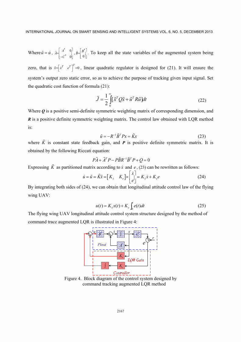
Whereu u , *

*

0

0

AA

C

,*

0

BB

. To keep all the state variables of the augmented system being

zero, that is 0TT Tx x e , linear quadratic regulator is designed for (21). It will ensure the

system’s output zero static error, so as to achieve the purpose of tracking given input signal. Set

the quadratic cost function of formula (21):

0

1[ ]

2T TJ x Qx u Ru dt

(22)

Where Q is a positive semi-definite symmetric weighting matrix of corresponding dimension, and

R is a positive definite symmetric weighting matrix. The control law obtained with LQR method

is:

1 Tu R B Px Kx (23) where K is constant state feedback gain, and P is positive definite symmetric matrix. It is

obtained by the following Riccati equation:

1 0T TPA A P PBR B P Q

Expressing K as partitioned matrix according to x and e , (23) can be rewritten as follows:

x e x e

xu u Kx K K K x K e

e

(24)

By integrating both sides of (24), we can obtain that longitudinal attitude control law of the flying

wing UAV:

0( ) ( ) ( )

t

x eu t K x t K e t dt (25)

The flying wing UAV longitudinal attitude control system structure designed by the method of

command trace augmented LQR is illustrated in Figure 4:

*A

*B *Cx x

xK

eK

u

re

Figure 4. Block diagram of the control system designed by

command tracking augmented LQR method


2168

It can be seen from Figure 4 that the output y of the model is feedback into the input of the

controller, and then get the error signal e(t) after being subtracted with a given input command.

Because the e(t) passes through the integrator, it can be judged that this control method can

eliminate the steady-state error of the system. Furthermore, this controller not only uses all the

state variables of the system, but also the output information. Therefore, it will predictably have a

good tracking effect.

b. Quasi-command tracking augmented LQR control method

When designing controller with the command tracking augmented LQR method, all the state

variables of the system have to be detected. However, some state variables are difficult or even

impossible to be directly detected in practical engineering applications, such as the angle of

attack. To this end, there is a quasi-command tracking augmented LQR method designed with

reduced-order observer. The specific process is discussed as follows.

Because the system (19) is completely observable, there must exist a linear transformation

x Tx which divides the state variables into two parts: one cannot be detected, the other can.

Here the transformation matrix1

0*

ZT

C

is selected, in which 0Z should ensure that T is non-

singular. The formula (19) will be transformed and divided as follows:

x Ax Bu

y Cx

(26)

where 1 2

Tx x x , 1x is the state vector that cannot be detected, and 2 [ ]x v q is

the state vector that can be detected. * 0C C T I , 1 * 11 12

21 22

A AA T A T

A A

, 1 * 1

2

BB T B

B

, 2y x . formula

(26) can be written as:

1 11 1 12 2 1

21 1 2 22 2 2

x A x A x B u

A x x A x B u

(27)

Set 12 2 1U A x B u , 2 22 2Y x A x B u , (3-9)can be rewritten as:

1 11 1

21 1

x A x U

Y A x

(28)


2169

U and Y are rectifiable based on known u and directly obtained 2x via y . Thus the state

reconstruction of the subsystem to be observed can be realized simply by designing a full-order

observer for (28). The full-dimensional observer designed by (28) is as follows:

1 11 21 1ˆ ˆ( )e ex A K A x K Y U

(29)

Where 1x is the estimated value of 1x , eK is the output error feedback matrix of state observer. By

substituting U and Y into (29), we obtain:

1 11 21 1 12 22 1 2ˆ ˆ( ) ( ) ( )e e e ex A K A x A K A y B K B u K y (30)

To eliminate y , the variable 1ˆ ˆ

ex K y is introduced and substituted into (30), we obtain:

11 21 12 22 11 21 1 2ˆ ˆ( ) [( ) ( ) ] ( )e e e e eA K A A K A A K A K y B K B u

(31)

Finally, combing with 1ˆ ˆ

ex K y , we obtain the estimated value of the entire state vector x as

follows:

1

2

ˆˆ ˆˆ0

eeI Kx K yx y

Ix y

(32)

Transforming (32) back to the original system, the state estimated value of the system (19) is

ˆx Tx .

As can be seen from (31) and (34), as long as the output error feedback matrix of the state

observer eK is obtained, it will be able to complete the design of reduced order observer. The

selection of the matrix eK will directly affect the convergence rate of the error 1e , where 1 1 1e x x .

For single-input systems, eK is generally obtained via the dual relationship between state

feedback and state observer. But for complex multi-input system, it will be more complex to

solve the state feedback matrix by pole assignment method. To this end, we choose conventional

LQR method to obtain eK . Firstly, the dual system of formula (28) is written as:

* * *

1 11 1 21

* *1

T Tx A x A U

Y x

(33)

Then we design linear quadratic regulator for (33), and solve the following Riccati equation:

111 11 21 21 0T TPA A P PA R A P Q (34)


2170

The feedback gain matrix can be obtained as * 121K R A P . Finally, we transpose matrix *K and

obtain 121( )

T T TeK K PA R .

Through the design of the reduced order observer, the state variable of the system that cannot

be detected can be estimated. So command tracking augmented LQR control method can be

adopted to design the longitudinal attitude control law of the UAV. We still set K as the

augmented LQR feedback matrix of the system (21) against the corresponding quadratic cost

function (22). Express K into block matrix 1 2x x eK K K K

according to 1x , 2x and e. Then

the longitudinal attitude control law of the flying wing UAV can be obtained as:

1 2ˆ 1 2 0ˆ( ) ( ) ( ) ( )

t

x x eu t K x t K x t K e t dt (35)

The structure of the flying wing UAV longitudinal attitude control system that designed by the

quasi-command tracking augmented LQR control method is illustrated in figure 5.

12 22eA K A

B C

A

eK

T

1 2eB K B

11 21eA K A

T

2 ,x y

cC

2 , ,x v q

( , )yy v

x x

r

1ˆx 1 ˆx

u

1xK

eK

2xK

e

u

Figure 5. Block diagram of the control system designed by quasi-command tracking augmented LQR method

V. DESIGN EXAMPLE

In this section, the longitudinal stability augmentation control law and the longitudinal attitude

control law of the flying wing UAV will be simulated. Now we research on the longitudinal of

the high-altitude long-endurance flying wing UAV, and select an altitude at 2000m, Mach 0.805


2171

as the typical state for analysis. The flying wing UAV is linearized in the flight state; the

augmented state equation and output equation are obtained as follows:

m m m m

m m m

x A x B u

y C x D u

(36)

Where Tm e t dx v q ， Tm e t du u u u

0.0127 6.2136 0 9.3718 0.0058 0.111 0.7384

0.004 1.9889 1 0.0411 0.0032 0.0002 0

0.0024 6.3838 2.4646 0 0.2437 0 0.3132

0 0 1 0 0 0 0

0 0 0 0 20 0 0

0 0 0 0 0 20 0

0 0 0 0 0 0 20

mA

0 0 0

0 0 0

0 0 0

0 0 0

20 0 0

0 20 0

0 0 40

mB

1 0 0 0 0 0 0

0 57.3 0 0 0 0 0

0 0 57.3 0 0 0 0

0 0 0 57.3 0 0 0

mC

0 0 0

0 0 0

0 0 0

0 0 0

mD

,

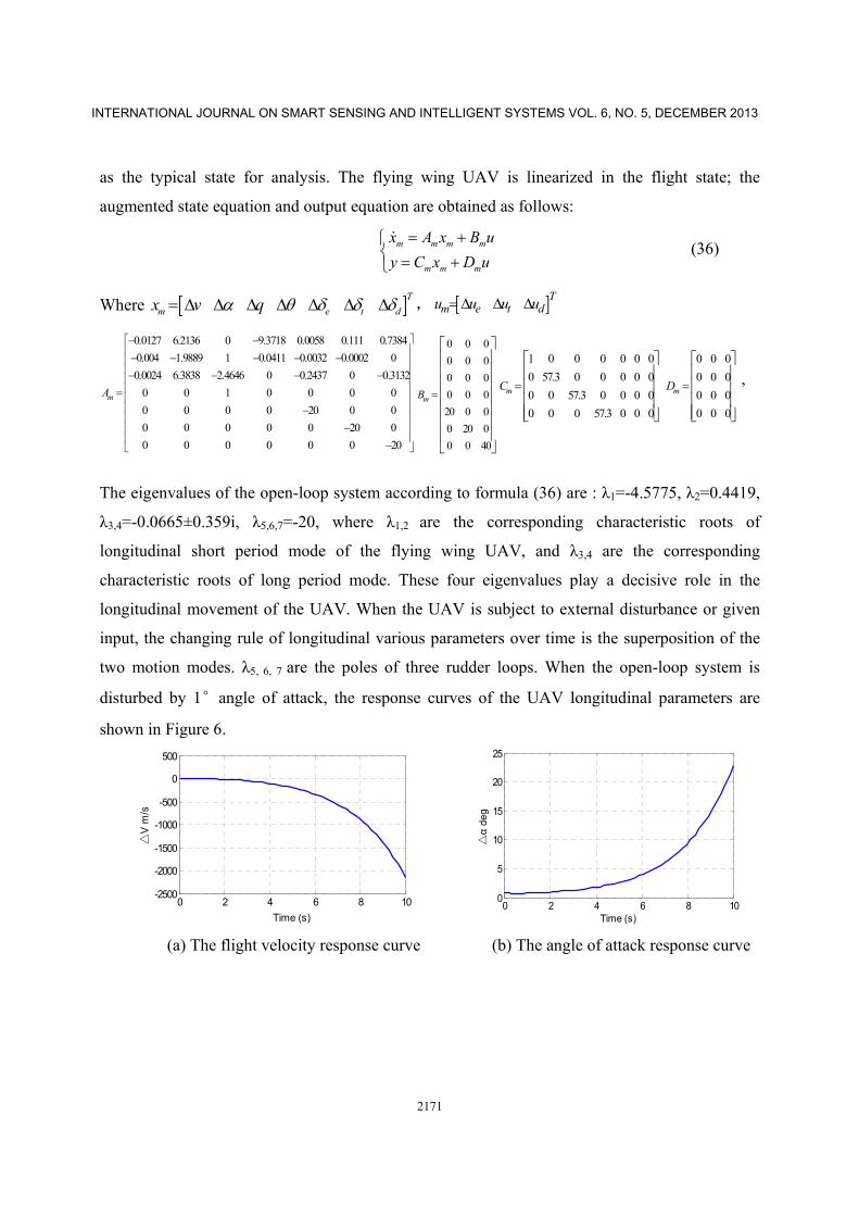
The eigenvalues of the open-loop system according to formula (36) are : λ1=-4.5775, λ2=0.4419,

λ3,4=-0.0665±0.359i, λ5,6,7=-20, where λ1,2 are the corresponding characteristic roots of

longitudinal short period mode of the flying wing UAV, and λ3,4 are the corresponding

characteristic roots of long period mode. These four eigenvalues play a decisive role in the

longitudinal movement of the UAV. When the UAV is subject to external disturbance or given

input, the changing rule of longitudinal various parameters over time is the superposition of the

two motion modes. λ5, 6, 7 are the poles of three rudder loops. When the open-loop system is

disturbed by 1°angle of attack, the response curves of the UAV longitudinal parameters are

shown in Figure 6.

0 2 4 6 8 10-2500

-2000

-1500

-1000

-500

0

500

Time (s)

V m

/s△

0 2 4 6 8 10

0

5

10

15

20

25

Time (s)

α d

eg△

(a) The flight velocity response curve (b) The angle of attack response curve


2172

0 2 4 6 8 100

10

20

30

40

50

60

Time (s)

q de

g/s

△

0 2 4 6 8 10

0

20

40

60

80

100

120

Time (s)

θ de

g△

(c) The pitch rate response curve (d) The pitch angle response curve

Figure 6. The disturbance response curve of the flying wing UAV before stability

Figure 6 shows that the response curves of the parameters are diverging after the UAV is

disturbed, because there exists the positive root in the UAV short period mode which is caused

by the flying wing UAV longitudinal static instability. Therefore, it is essential to conduct

longitudinal stability augmentation control for the flying wing UAV.

The longitudinal stability augmentation control law of the UAV，can be designed as u=Ky by

use the output feedback linear quadratic regulator, where 3 4K R . In order to get a satisfying

stability augmentation effect, the appropriate weighting matrices Q and R augmentation should

be firstly selected before the output feedback by LQR application. Considering that the UAV

longitudinal static instability will lead to the short period mode of the UAV diffuse, in the

quadratic cost function, the state Δα2 andΔq2 which are closely relevant to short period mode

should be weighted by element qα of the weighting matrix Q if we want to obtain the short period

mode with a satisfying stability. In the long period mode, under damping can be seen from the

characteristic values λ3, 4, it is necessary for the state Δv2 and Δθ2 which are closely relevant to

the long period mode, to be weighted by the element q b of the weighting matrix Q. As the

extended state variables are not discussed, there is no need to weight them. As a result, the

weighting matrix Q can be rewritten as Q=diag{qb,qa,qa,qb,0,0,0}. In terms of R, the form of R=ρ

×I is used to prevent oversize control input. Where is the design parameter and I is a unit

matrix of corresponding dimension.

After selecting and checking repeatedly, it can be concluded that the longitudinal stability

augmentation of the UAV will achieve the best when Q=diag{50,10,10,50,0,0,0} and ρ=1. The


2173

optimal feedback matrix K is obtained as follows by the use of the iterative solution method

mentioned in section Ⅲ:

1.6073 22.8329 23.3958 26.5004

7.2136 10.1877 0.9967 14.1970

3.2225 2.4844 2.4463 7.6770

K

0 10 20 30 40 50 60 700

500

1000

1500

2000

Iterative times

Qua

drat

ic c

ost f

unct

ion

J

Figure 7. The changing curve of the quadratic cost function J

The changing curve of quadratic cost function during iterative process is illustrated in Figure 7.

The eigenvalues of the closed-loop system after stability augmentation are λ1,2=-1.526±0.764i,

λ3,4=-10.437±9.01i, λ5=-5.884, λ6=-14.657, λ7=-20. When the closed-loop system is disturbed by

1°angle of attack, the response curves of the UAV longitudinal parameters are shown in Figure

8.It can be seen from Figure 8 and the closed-loop system characteristic roots, the longitudinal

dynamic quality of the flying wing UAV after stability augmentation has improved significantly.

0 2 4 6 8 10-0.2

-0.15

-0.1

-0.05

0

0.05

0.1

0.15

Time (s)

V m

/s△

0 2 4 6 8 10

-0.2

0

0.2

0.4

0.6

0.8

1

1.2

Time (s)

α d

eg△

(a).The flight velocity response curve (b).The angle of attack response curve


2174

0 2 4 6 8 10

-0.1

0

0.1

0.2

0.3

Time (s)

q de

g/s

△

0 2 4 6 8 10

-0.02

0

0.02

0.04

0.06

0.08

0.1

Time (s)

θ de

g△

(c).The pitch rate response curve (d).The pitch angle response curve

Figure 8. The disturbance response curve of the flying wing UAV after stability augmentation

We have achieved the stability augmentation control, the longitudinal attitude control will be

completed based on it. In order to verify the two kinds of attitude control methods mentioned in

the third section, here we only control the flight velocity and the pitch angle. The stability

augmented Δv and Δθ are chosen as the system output and ut, ue are chosen as the system control

input. The two augmented LQR control methods mentioned in the third section are applied to

design the attitude control law ut and ue, so that the command tracking of the flight velocity and

pitch angle can be achieved. It is assumed that all the states of the system are measurable when

we use command tracing augmented LQR method to design the control laws. While the angle of

attack which is assumed immeasurable can be estimated by the reduced order observer when the

command tracking augmented LQR method is adopted to design the control laws.

The state equation and output equation of the flying wing UAV after stability augmentation are：

( ) ( ) ( )

( ) ( )

x t A x t B u t

y t C x t

(37)

Where Te tx v q , Tt eu u u , Ty v . According to the methods in

Section Ⅳ.a, equation (37) can achieve a new augmented state equation：

x Ax Bu (38)

Select quadratic cost function (22) and design the linear quadratic regulator for (38). After

selecting and checking repeatedly, it can be concluded that the command trace will achieve the

best when R=diag{1,1}, Q=diag{20,20,20,20,1,1,500,2000}. The optimal feedback matrix K is

obtained as follows：


2175

14.59 90.15 90.17 380.32 4.77 0.012 7.89 185.56

27.22 62.95 8.57 116.62 0.018 3.62 11.75 124.75

t t t t t t t t

ve t

e e e e e e e e

ve t

u u u u u u u uv a q e e

u u u u u u u uv a q e e

k k k k k k k kK

k k k k k k k k

Finally, the flying wing UAV flight velocity and pitch angle control laws are designed by the

command tracking augmented LQR method：

t t t t

t t t t

ve t

e e e e

e e e e

ve t

u u u uv t v a q

u u u ue t e v e

u u u ue v a q

u u u ue t e v e

u u k v k a k q k

k k k e dt k e dt

u u k v k a k q k

k k k e dt k e dt

(39)

When quasi-command tracking augmented LQR method is used to design attitude control laws,

in addition to design the reduced order observer for the state variable that cannot be detected,

the rest of the design process is exactly the same with the above. To this end, there is no longer

detailed description. Equation (37) is designed according to the reduced order observer in section

Ⅳ.b, the output error feedback matrix of state observer is 0.3615 0.3714 0eK . Finally,

the flying wing UAV flight velocity and pitch angle control laws are designed by the quasi-

command tracking augmented LQR method：

ˆ

ˆ

t t t t

t t t t

ve t

e e e e

e e e e

ve t

u u u uv t v a q

u u u ue t e v e

u u u ue v a q

u u u ue t e v e

u u k v k a k q k

k k k e dt k e dt

u u k v k a k q k

k k k e dt k e dt

(40)

We will use the two groups of attitude control laws to conduct simulation to the UAV

longitudinal linear model. In order to simplify the following expressions, set the formula (39) as

the controller ① and the formula (40) as the controller ②. Now the flying wing UAV linear

model is selected when the flight status is h=2000m，Ma=0.805. Assume that the initial state of

the linear model is an equilibrium state. when the simulation time t = 1s, the flight velocity will

be given a step signal of 50m/s and the pitch angle will be given a step signal of 5°. The

simulation results are shown in Figure 9 and Figure 10.


2176

0 5 10 15 20 25 30 350

10

20

30

40

50

60

Time (s)

V m

/s△

Input commandSystem output

0 5 10 15 20 25 30 35

0

1

2

3

4

5

6

Time (s)

θ de

g△


(a) The flight velocity step response curve (b) The pitch angle step response curve

Figure 9. Simulation results with controller ①

0 5 10 15 20 25 30 350

10

20

30

40

50

60

Time (s)

V m

/s△


0 5 10 15 20 25 30 35

0

1

2

3

4

5

6

Time (s)

θ de

g△


(a) The flight velocity step response curve (b) The pitch angle step response curve

Figure 10. Simulation results with controller ②

Figure 9, 10 show that the two controllers are able to make the input signals be tracked without

steady-state error. Meanwhile, there is high adjusting precision, short transition time and small

overshoot in the response process. As reduced order observer is introduced in controller②, in

order to analyze the effect on the command tracking augmented LQR control by the reduced

order observer, we make the difference between figures 9 and 10, and then obtain system output

difference curves of the two control methods, which are shown in Figure 11：


2177

0 5 10 15 20 25 30 35-0.6

-0.4

-0.2

0

0.2

0.4

0.6

0.8

Time (s)

V m

/s△

0 5 10 15 20 25 30 35

-0.6

-0.5

-0.4

-0.3

-0.2

-0.1

0

0.1

Time (s)

θ de

g△

(a) The flight velocity difference curve (b) The pitch angle difference curve

Figure 11. The system outputs difference curve of two control methods

0 5 10 15 20 25 30 350

5

10

15

20

25

30

35

40

Time (s)

V m

/s△

controller①controller②

0 5 10 15 20 25 30 35

-0.7

-0.6

-0.5

-0.4

-0.3

-0.2

-0.1

0

0.1

Time (s)

θ de

g△


(a) The flight velocity response curve (b) The pitch angle disturbance curve

Figure 12. The velocity loop step response curve

0 5 10 15 20 25 30 350

0.5

1

1.5

2

2.5

3

3.5

4

Time (s)

θ de

g△

controller①

controller②

0 5 10 15 20 25 30 35

-1.5

-1

-0.5

0

0.5

1

Time (s)

V m

/s△


(a) The pitch angle response curve (b) The flight velocity disturbance curve

Figure 13. The pitch angle loop step response curve

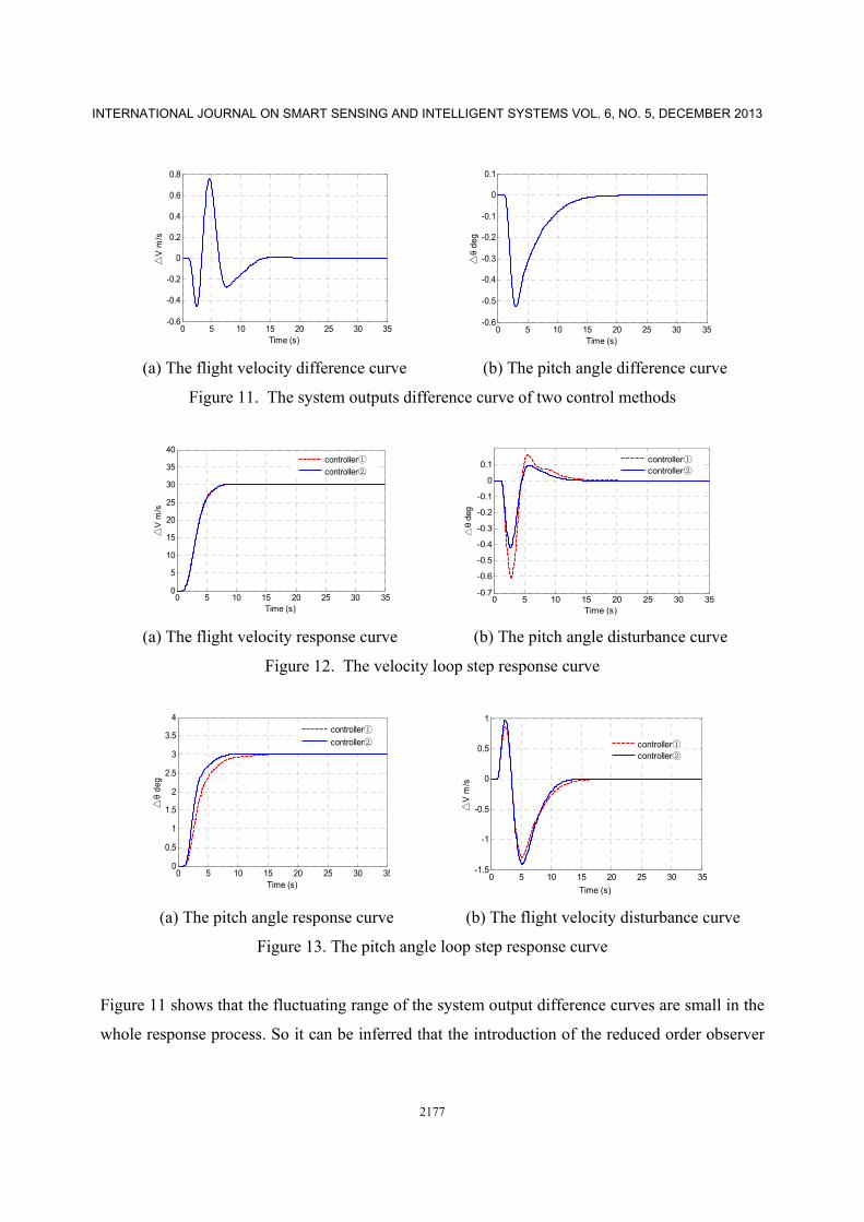
Figure 11 shows that the fluctuating range of the system output difference curves are small in the

whole response process. So it can be inferred that the introduction of the reduced order observer


2178

make little effect on command tracking augmented LQR, and the controller ② almost keep the

full performance of the controller ①.

In order to verify the decoupling performance of the two controllers，the same controlled model

as above will be selected, the flying speed will be given a step signal of 30m / s and the pitch

angle will be given a step signal of 3°. The simulation results are shown in figure 12 and figure

13.

Figure.12 shows that when speed is controlled only, the maximum disturbance of the pitch angle

is less than 0.7, and the disturbance is 0 after 15s. Figure.13 shows that when pitch angle is

controlled only, the maximum disturbance of the speed is less than 1.5m/s, the disturbance

becomes 0 after 15s. Therefore, both controllers have strong decoupling performance.

0 5 10 15 20 25 30 35 4040

42

44

46

48

50

52

Time (s)

V m

/s△

controller①

controller②

0 5 10 15 20 25 30 35 40

0

0.5

1

1.5

2

2.5

3

3.5

4

Time (s)

θ de

g△

controller①

controller②

(a) The flight velocity response curve (b) The pitch angle response curve

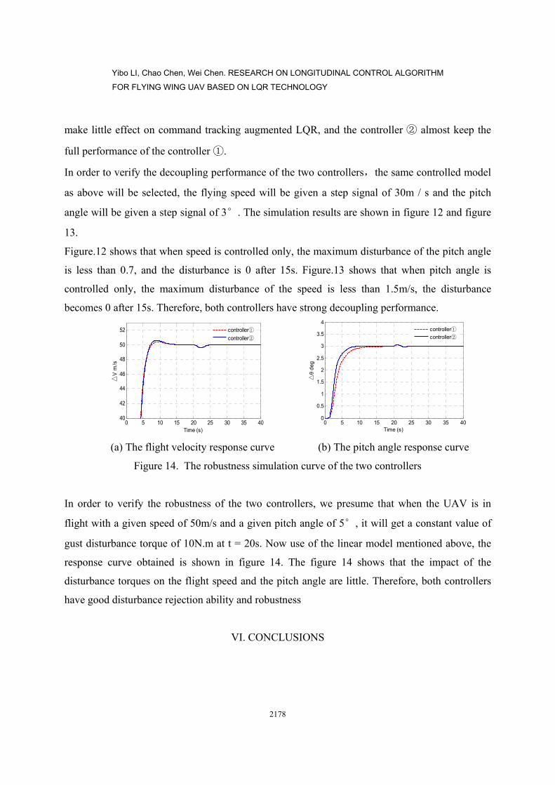
Figure 14. The robustness simulation curve of the two controllers

In order to verify the robustness of the two controllers, we presume that when the UAV is in

flight with a given speed of 50m/s and a given pitch angle of 5°, it will get a constant value of

gust disturbance torque of 10N.m at t = 20s. Now use of the linear model mentioned above, the

response curve obtained is shown in figure 14. The figure 14 shows that the impact of the

disturbance torques on the flight speed and the pitch angle are little. Therefore, both controllers

have good disturbance rejection ability and robustness

VI. CONCLUSIONS


2179

In this paper, we take high-altitude long-endurance flying wing UAV as a platform. First of all,

longitudinal mathematical model is established based on its special aerodynamic layout and

unique control surfaces. Then we combine LQR technology to design the longitudinal stability

augmentation control law and the attitude control law of the UAV respectively. The stability

augmentation control is achieved by using output feedback linear quadratic method that not only

improve the longitudinal static stability and the dynamic characteristics, but also reduce the

numbers of feedback compared with conventional LQR state regulator. The attitude control law

of the flying wing UAV uses a special control system augmented method and conventional LQR

method to obtain a command tracking augmented LQR method. The simulation results show that

the control law effectively realizes the command tracking of the angle of pitch and the flight

velocity. Besides, the controller has strong robustness and decoupling performance. It can be seen

from the time domain performances of the control system that the overshoot, the accommodation

time and the steady accuracy are very ideal. Finally, when the system state variables can not be

detected all, we also designed quasi-command tracking augmented LQR control method. It

retains all the features of command tracking augmented LQR control method and more suitable

for the application of practice engineering. Above all, the simulation results show that the

longitudinal control laws of the flying wing UAV based on LQR enable the UAV to achieve

satisfactory longitudinal flying quality.

REFERENCES

[1] R.M. Wood and X.S. Bauer, “Flying wings/flying fuselages”, AIAA paper 2001-0311,

January 2001, pp. 1-7.

[2] W.R. Sear, “Flying Wing airplanes-The XB-35/YB-49 program”, AIAA paper 80-3036 in

Evolution of Aircraft Wing Design Sytnposium, pp. 57-59, March 1980.

[3] S. Esteban, “Static and dynamic analysis of analysis of an unconventional plane flying wing”,

AIAA Atmospheric Flight Mechanics Conference and Exhibit, Montreal, Canada. August 2001,

pp. 6-9.

[4] A.R. Weyl, “Tailless Aircraft and Flying Wings A Study of Their Evolution and Their

Problems”, Aircraft Engineering, vol. 16, No. 5, pp. 8-13, January 1945.


2180

[5] G. Yang, J.G. Sun and Q.H. Li, “Augmented LQR Method for Aeroengine Control Systems”,

Journal of Aerospace Power, vol. 19, No. 1, pp. 153-158, February 2004.

[6] W.K. Lai, M. F. Rahmat and N.A. Wahab, “Modeling and controller design of pneumatic

actuator system with control valve”, International Journal on Smart Sensing and Intelligent

Systems, vol. 5, No. 3, pp. 624-644, September 2012.

[7] R. Ghazali, M. Rahmat, Z. Zulfatman et al., “Perfect tracking control with discrete-time lqr

for a non-minimum phase electro-hydraulic actuator system”. International Journal on Smart

Sensing and Intelligent Systems, vol. 4, No. 3, pp.424-439, September 2011.

[8] L. Gargouri, A. Zaafouri and A. Kochbati et al., “LQG／LTR Control of a Direct Current

Motor”, Systems, Man and Cybernetics, 2002 IEEE International Conference on. IEEE, vol. 5, pp.

5-10, May 2002.

[9] O. Rehman, B. Fidan and I.R. Petersen, “Minimax LQR control design for a hypersonic flight

vehicle”, 16th AIAA/DLR/DGLR International Space Planes and Hypersonic Systems and

Technologies Conference, October 2009.

[10] R.W. Huang and Y.D Zhao, “Soft landing control of electromagnetic Valve actuation for

engines by using LQR”, Tsinghua Science and Technology, vol. 47, No. 8, 2007, pp. 1338-1342.

[11] S.B. McCamish, M. Romano and S. Nolet et al., “Flight testing of multiple-spacecraft

control on SPHERES during close-proximity operations”, Journal of Spacecraft and Rockets, vol.

46, No. 6, pp. 1202-1213, November–December 2009.

[12] X.J. Xing, J.G. Yan and D.L. Yuan, “Augmented-stability controller design and its

simulation or a UAV based on LQR theory”, Flight Dynamics, vol. 29, No. 5, pp. 54-56,

October 2011.

[13] J.W. Choi, G. Daniel and L.R. Mariano, “Control System Modeling and Design for a Mars

Flyer, MACH-1 Competition”, AIAA Guidance, Navigation and Control Conference and Exhibit,

Honolulu, Hawaii, August 2008.

[14] Y. Tao, “Application of Explicit-Model Following Control technology in the Attitude

Control System for the Unmanned Shipboard Helicopter”, Journal of Naval Aeronautical

Engineering Institute, vol. 24, No. 5, pp. 543-546. September 2009.


2181

[15] J. Andersson, P. Krus and K. Nilsson, “Optimization as a support for selection and design of

aircraft actuation systems”, Proceedings of Seventh AIAA/USAF/NASA/ISSMO Symposium on

Multidisciplinary Analysis and Optimization, St. Louis, USA, September 1998.

[16] Y.B. Li, W.Z. Liu and Q. Song, “Improved LQG control for unmanned helicopter based on

active model in wind environment”, Flight Dynamics, vol. 30, No. 4, pp. 318-322, August 2012.

[17] L. Zhang and Z. Zhou, “Study on Longitudinal Control Laws for High Altitude Long

Endurance Tailless Flying-wing Unmanned Aerial Vehicles”, Science Technology and

Engineering, vol. 7, No. 16, pp. 1671-1819, August 2007.

[18] M.L. Zhang, “Flight Control System”, National defense of Industry Press, 2nd edn, pp. 41-

42, 1994.

[19] E.Q. Yang, “Research on the key technology of Unmanned Combat Aerial Vehicle flight

control system”, Ph.D. Dissertation, Automation Science and Electrical Engineering Dept.

Beijing Univ. of Aeronautics and Astronautics, Beijing, China, May 2006.

[20] G. Garcia, J. Daafouz and J. Bernussou, “Output Feedback Disk Pole Assignment for

Systems with Positive Real Uncertainty”, Automatic Control, IEEE Transactions on, vol. 41, No.

9, 1996, pp. 1385-1391.

[21] D.E. Miller and M. Rossi, “Simultaneous Stabilization With Near Optimal LQR

Performance”, Automatic Control, IEEE Transactions on, vol. 46, No. 10, 2001, pp. 1543-1555.

[22] D.D. Moerder and A. Calise, “Convergence of a Numerical Algorithm for Calculating

Optimal Output Feedback Gains”, Automatic Control, IEEE Transactions on, vol. 30, No. 9,

1985, pp. 900-903.

RESEARCH ON LONGITUDINAL CONTROL ALGORITHM FOR FLYING WING UAV BASED ON LQR...

Documents

Transcript of RESEARCH ON LONGITUDINAL CONTROL ALGORITHM FOR FLYING WING UAV BASED ON LQR...