Research on Brain-inspired Vision Based on Dynamic Vision ...

Research on Brain-inspired Vision Based on

Dynamic Vision Sensor Cameras Xiuxiu Zhang, Guowen Xiao, Sibo Gui, Quansheng Ren*

Electronics and Systems

Peking University

Beijing, China

{zhangxiuxiu, 1801213557}@pku.edu.cn, [email protected], [email protected]

Abstract—In this paper, we explored many applications of

brain-inspired vision, in which the data was acquired based on

a dynamic vision sensor camera, that is PSEE300EVK from

French. Specifically, we explored the following three aspects: (1)

Converting large-scale artificial convolution neural network

into spiking neural network, which can process large-scale

datasets and save network resources without dropping much

precision. We proposed reliable solutions for the difference

between the two networks, and it can be generalized to other

deep network transformations. (2) Recognizing pedestrians and

vehicles spiking data flow in the autopilot scenario. Specifically,

we transformed Cityscapes dataset into two modes spiking data,

one called event processing mode, another called contrast

detection mode. (3) Constructing a structured light 3D

acquisition system and 3D image recognition algorithm based on

the PSE300EVK camera. Tests show that the algorithm used in

this paper can effectively reduce the error between the deep

artificial convolutional neural network and the deep spiking

convolutional neural network, and it has good ability of

generalization, and the algorithm can effectively process spiking

images and 3D images.

Keywords—brain-inspired vision, dynamic vision sensor,

spiking neural network, 3D

I. INTRODUCTION

The purpose of brain-inspired computing is to synthesize neuroscience, cognitive science, and information science to explore how biological nervous systems achieve intelligence, and then build artificial intelligence systems to simulate biological nervous systems. Unlike traditional artificial intelligence, brain-inspired computing is based on a large number of neuroscience theories and experimental results. It uses spiking neural network which is used by the biological brain to work in an asynchronous, event-driven manner, which can better learn from biological neurons. It hopes to promote the research of brain nerve in the field of neuroscience at the same time. Meanwhile, the spiking neural network used by the biological brain is easier to implement distributed computing and information storage on the hardware, can process non-precision and unstructured data such as multi-sensory cross-modality in real time, and hope to realize general artificial intelligence. After nearly 30 years of development, brain-inspired computing has received great attention from the research community and has also achieved some related achievements, but it still faces huge difficulties and challenges on some more complex issues and actual industrial production. And because humans perceive the external environment mainly through sensory systems such as sight, hearing, touch, smell and taste, among which the visual system occupies the largest proportion and is the most complicated. Humans obtain the largest amount of visual

signals from the outside world, so this article will explore the application of brain-inspired computing in all aspects of the visual field.

In order to build an end-to-end brain-inspired vision system, this article uses a more biomimetic brain-inspired vision camera. Inspired neuronal transmission biological retina information mode, the DVS[1] ( Dynamic Vision Sensor) camera taken on AER[2](Address Event Representation) in asynchronous transfer mode, only when an "event" occurs, the sensor outputs the "event" and the address of the "event". The DVS camera used in this article is produced by the French company Prophesee[3], which uses the CSD3SVCD photosensitive chip. Based on the event information, each pixel accumulates a certain light intensity and sends a pulse backward. It uses a time resolution of 1us, which provides a new solution for us to see and understand some objects that are too dark, overexposed or moving too fast. At the same time, it has a spatial resolution of 640*480, and can simultaneously use CD (Contrast Detection) and EM (Event Processing) modes. The former sends pulses backward based on dynamic change information, which can greatly reduce the amount of data; the latter is based on cumulative light intensity Sending information backwards can realize asynchronous processing and speed up the processing of visual information. At the same time, because the output of DVS is a series of pulses, rather than the traditional pixel matrix-based image frame, the traditional signal and image processing algorithms are not applicable, and a new back-end brain-inspired algorithm needs to be designed.

Neural network algorithms are now occupying an important position in people's daily lives. The first-generation neural network is the perceptron, which is a simple neuron model and can only process binary data. The second-generation neural network includes more extensive, the most common is the back-propagation neural network[4], hereinafter referred to as direct artificial neural networks or traditional artificial neural networks. These networks are encoded based on the frequency of nerve impulses. Among them, the convolutional neural network[5] used in the field of image processing is even more brilliant. In recent years, convolutional neural networks are widely used to process various visual information, which can be regarded as a simple imitation of the animal visual system. They are widely used in the fields of general target detection, pedestrian detection, face recognition, image semantic segmentation, video classification, key location detection and target tracking.

However, the development of convolutional neural networks has its own shortcomings, such as poor

interpretability and inability to perform causal reasoning. Secondly, it cannot handle asynchronous high-resolution events generated by the PSEE300EVK camera well. Therefore, we combine the characteristics of the camera data and use a spiking neural network[6] to deal with brain-inspired vision problems. Compared to artificial neural networks, spiking neural networks have a stronger biological basis, is often hailed as the three generations of artificial neural network, which is more realistic simulated neurons, in addition, the influence of time information is also considered, which cannot be expressed by traditional artificial neural networks. During operation, the neurons in the dynamic neural network are not activated in each iteration of propagation, but only when its membrane potential reaches a certain threshold. When a neuron is activated, it will produce a signal to other neurons to increase or decrease its membrane potential. So it will have lower power consumption and higher computing speed.

However, the research on the learning algorithm of spiking neural network is not perfect. At present, the academic and industrial circles mainly study the spiking neural algorithm from two aspects: one is to find the effective learning mechanism; the other is how to apply the spiking neural network to practical work. In my research direction, the main consideration is the second point, using impulse neural network to process brain-inspired visual information efficiently

II. DVS CAMERAS

For a traditional camera, it uses a detector to simultaneously sample a series of still images. The processing method for video is to capture a series of still images and quickly replay, then this series of images will give the viewer a sense of movement. For objects that move too fast, we need a large number of frames to track the movement correctly, which is a huge burden on storage devices and analysis processing equipment. For information we not interest, there is a lot of redundancy in the data; and for information of interest, we often prefer a higher frame rate; therefore, there is both oversampling and undersampling in this process. Therefore, for some complex problems, we envisage solving them with some asynchronous cameras.

For the human eye, if the object moves too fast, we cannot see the specific details, but we are naturally sensitive to the amount of change. So neuromorphic bio-inspired systems to create a more efficient electronic signal processing system in which information collection part will be based on the shortcomings of traditional cameras, for different parts of the scene to sample in different rates. The part of the scene that contains fast motion will be quickly sampled, while the part that changes slowly will be sampled at a lower rate, and if there is no change, it will be reduced to zero.

The Prophesee camera used in this article is inspired by the biology of the eye and brain. Each pixel is connected to a horizontal cross detector and a separate exposure measurement circuit. For individual pixels, the electronic device detects that the signal amplitude of the pixel is suitably higher or lower than the previous amplitude, and then records the new signal value at this point. In this way, each pixel will optimize its own sampling according to the change of received light. Based on the above principle, if the light reaching a pixel changes rapidly, then the pixel will be sampled frequently. If there is no change, the pixel stops

transmitting redundant information backwards and enters an idle state until a new event occurs in the area. The circuit associated with the pixel immediately outputs a new measurement value when it detects a change, and it can Track the position of the changing pixel in the sensor array. These outputs are encoded according to the protocol of geological event representation, so we often call this camera an event-driven camera, which sends asynchronous pulses backward.

Chip for each pixel of the change detector is based on a fast and asynchronous event-driven continuous-time signal processing logarithmic photoreceptor. It continuously monitors changes in the optical flow, and to give a response to the polarity change events, these events is the relative increase or decrease in the light intensity exceeds a set value threshold. The occurrence of these events is detected by one of the two voltage comparators. The event generating circuit responds to the positive and negative slopes of the photocurrent with positive or negative pulse events, respectively. When the change exceeds the threshold, a pulse is excited in response to the pixel, and the voltage returns to the original position.

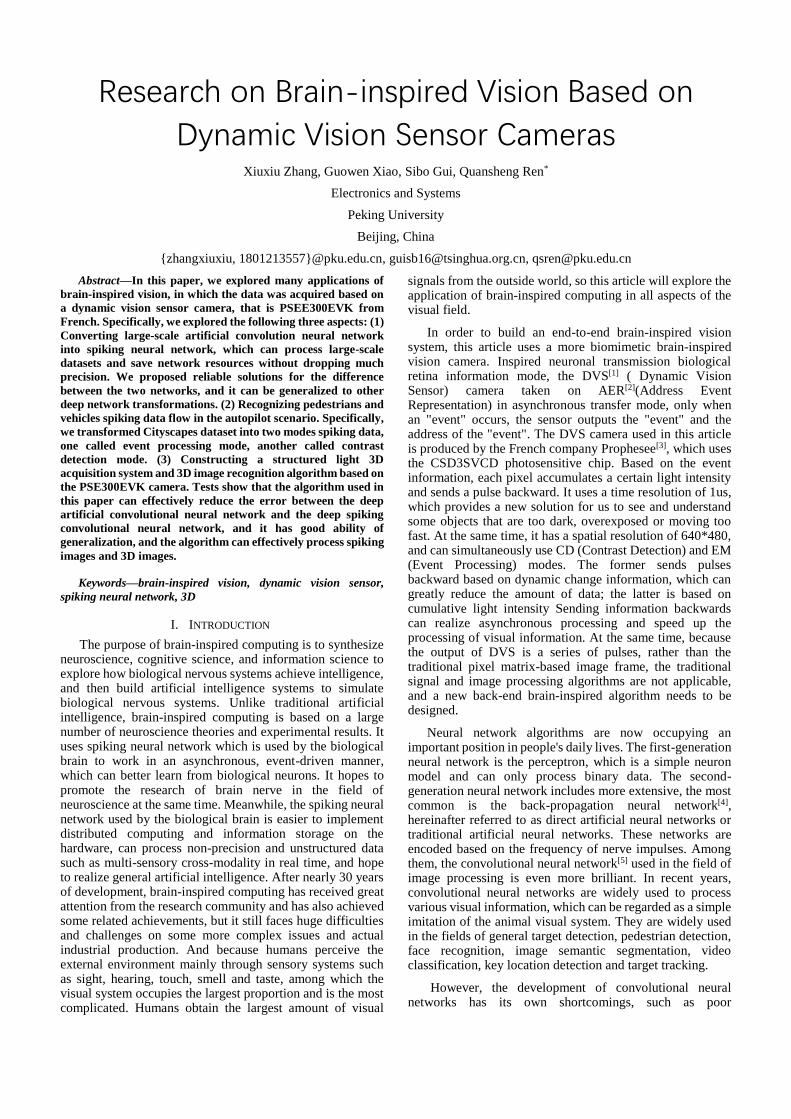
As shown in Fig.1., it is the Prophesee camera. His vision sensor comprising mentioned above, a standard C lens mount, the lens can be replaced according to actual needs, and a USB 3.0 in the external interfaces.

Fig. 1. Prophesee camera

We use prophesee_player software to acquire the data, the computer software has following requirements: containing the USB 3.0 interface, and 64-bit Win10 systems or Linux Ubuntu 16.04 or 18.04 system. With this camera, we can provide higher speed, greater dynamic range and save computing costs. At the same time, in order to process these data more efficiently, we need to redesign the program to apply the data. Based on this starting point, we design efficient processing methods for spike data streams in various scenarios.

III. CONVERTING DEEP ARTIFICIAL CONVOLUTIONAL NEURAL

NETWORK TO SPIKING NEURAL NETWORK

With the rapid development of deep learning, the performance of artificial neural networks(ANN) on various tasks has become increasingly noticeable. At the same time, the defects of ANN are gradually revealed. If the artificial neural network is not interpretable, people cannot understand the principle why it can work so efficiently, so it is not safe to use for some projects with high safety requirements, such as medical treatment. At the same time, as the network scale is getting deeper, the requirements for memory and computing power are getting higher and higher and the delay is also increasing, which also makes it more difficult to integrate into some fixed devices (such as mobile phones). The spiking

neural network provides new ideas for solving these problems. However, the development of spiking neural networks is not mature enough at present, and because of its discretization characteristics, it cannot carry out back propagation training. Therefore, the existing small-scale SNNs are basically doing some algorithm innovations, so in some practical scenarios the following applications are limited. Therefore, this chapter mainly expects to transplant the large-scale convolutional neural network to the spiking neural network to minimize its loss in accuracy while exerting its advantages. In this part, we selected the common model of natural scene classification VGGNet[7] and tested it on the large-scale natural scene picture dataset CIFAR-10[8], and it is foreseeable that using this algorithm can convert large-scale spiking neural networks into their corresponding spiking neural networks.

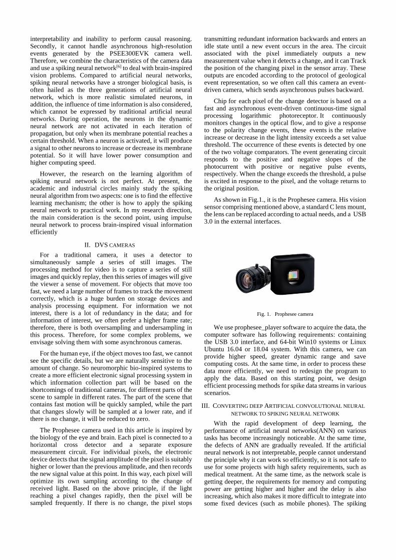
VGGNet was proposed by the group of Oxford ’s Visual Geometry Group, which improved the accuracy in the ILSVRC series competition, and proved that increasing the depth of the network to a certain extent can improve the performance of the network. As shown in Fig.2., there are six common structures in VGGNet. From left to right in the figure, the number of layers is gradually deepened. In addition to the A-LRN structure, each structure consists of convolution - pooling – fully - connected - softmax layers. One of the most commonly used is the structure of D, also known as VGG 16, which means that it has 16 layers.

Fig. 2. VGGNet structures

There are two main differences between the ANN network and the SNN network. One is the form of data stream. In traditional artificial neural networks, it is simulated numerical value, while in spiking neural network, it is spiking data stream, which is expressed as 0 and 1 in mathematics. The second is the network transmission rules. In ANN, neurons transfer calculations of their activation values backward, while in spiking neural networks, the membrane potential of each neuron is only a transient value. Only after it reaches the threshold value will a pulse be transmitted backward. The membrane potential of this neuron will be reset. In order to reduce the error between the conversion of ANN to SNN, our ideal situation is to make a one-to-one mapping between SNN unit and ANN unit. Therefore, the basic principle we follow is to match the firing frequency of pulse neurons with the non-linear activation value of ANN. Based on this theory, some formulas are explained below. First of all, for ANN, we define the activation value of the first neuron in the layer

𝑎𝑖𝑙 = max(0, ∑ 𝑊𝑖𝑗

𝑙𝑗=1 𝑎𝑗

𝑙−1 + 𝑏𝑖𝑙) ()

Here, we make𝑎0 = 𝑥, which 𝑥 represents the normalized result of the input layer, i.e. 𝑥 ∈ [0,1].Then for the spiking neural network, the voltage of the i-th neuron in the lth layer increases after each time step is

bwz

l

i

l

jij

l

ij

l

i

Mt

l

+= −

=

−

1

,1

1

)(

()

𝜃𝑖,𝑗𝑙−1 represents time t if i-th neuron received transmission

spike neurons from j-th neuron, having value of 0 or 1, which

means not transmitted pulse overshoot or transmit pulses,

respectively. For a period of time T, we set each time step as

∆t, then the highest pulse emissivity is 𝑟𝑚𝑎𝑥 = 1/∆𝑡, that is,

at most one pulse is sent within a time step. Then we define

the firing rate of the i-th neuron is 𝑟𝑖𝑙(𝑡) = 𝑁𝑖

𝑙(𝑡)/𝑡, where

represents the cumulative firing pulses from the beginning to

time t.So when 𝑟𝑖𝑙 is proportional to 𝑎𝑖

𝑙 , we can get the

minimum converting error.

A. Input conversion

According to the different types of network data streams, first we have to convert the input analog values of ANN into spiking data streams. Here we use the form of Poisson division to convert RGB pixels into pulse values at corresponding frequencies. Poisson distribution is a common discrete probability distribution model, which represents the number of random events that occur over a period of time. Suppose the pixel value of a point is γ, average of the number of spikes within the time ∆t should be γ∆t. Then at every time step, the probability of issuing a pulse is p(x = 1) ≈ γ∆t .Then generate a random number between 0 and 1 at each time step, if the random number is less than or equal to γ∆t, then send a pulse backward. Otherwise, no pulse is sent. In this way, it can be converted into corresponding pulse data according to the actual pixel value. And when the time interval is small enough, the original pixel value can be restored.

B. Reset

When the neuron's membrane potential exceeds the threshold, it sends a pulse backward, and at the same time, the neuron's membrane potential will be reset. Generally speaking, there are two different reset mechanisms. One is to directly reset to 0, and the other is to subtract the threshold. The rationality of the two mechanisms will be explained below through mathematical formulas.

First we define 𝑉𝑖𝑙(𝑡) as time t l-th layer i-th neuron

membrane potential, 𝑧𝑖𝑙(𝑡)as time t of l-th layer i-th neuron’s

voltage increase because of the foregoing neurons,

𝜃𝑖𝑙(𝑡)represented time t of l-th layer i-th neuron whether to

transmit pulses. At the same time, for the convenience of

calculation, we recalculate 𝑧𝑖𝑙(𝑡) = 𝑉𝑡ℎ𝑟(𝑧𝑖

𝑙(𝑡)) , which 𝑉𝑡ℎ𝑟 represents the membrane potential threshold, this

function represents the modulus 𝑉𝑡ℎ𝑟 . This can get 𝑧𝑖𝑙(𝑡) ∈

[0,𝑉𝑡ℎ𝑟)， 𝑉𝑖𝑙(𝑡) ∈ [0,𝑉𝑡ℎ𝑟). Then we can get two mode:

𝑉𝑖𝑙(𝑡) = {

(𝑉𝑖𝑙(𝑡 − 1) + 𝑧𝑖

𝑙(𝑡)) (1 − 𝜃𝑖𝑙(𝑡)) 𝑟𝑒𝑠𝑒𝑡𝑡𝑜0

𝑉𝑖𝑙(𝑡 − 1) + 𝑧𝑖

𝑙(𝑡) − 𝑉𝑡ℎ𝑟𝜃𝑖𝑙(𝑡)resetbysubtract

()

Let's simplify the calculation through the first layer, because the first layer does not involve convolution operations, the two inputs are the same, and for the convenience of writing, we remove the concept of layer and neuron here.

Then for the mechanism of resetting to 0, the cumulative membrane potential within the simulation time t can be written as

∑ 𝑉(𝑡0) =𝑡𝑡0=1 ∑ (𝑉(𝑡0 − 1)𝑡

𝑡0=1 + 𝑧)(1 − 𝜃(𝑡0)) ()

And 𝑁(𝑡) = ∑ 𝜃(𝑡0)𝑡𝑡0=1 ，∑ 1 = 𝑡/∆𝑡𝑡

𝑡0=1 , that is a

total of so many time steps. 𝑟𝑚𝑎𝑥 = 1/∆𝑡 Will be substituted into the above formula

𝑟(𝑡) =𝑁(𝑡)

𝑡=𝑟𝑚𝑎𝑥 −

1

𝑧𝑡∑ (𝑉(𝑡0) − 𝑉(𝑡0 − 1)𝑡𝑡0=1 )(1 −

𝜃(𝑡0)) ()

And because of the ∑ (𝑉(𝑡0) − 𝑉(𝑡0 − 1)) = 𝑉(𝑡) −𝑡𝑡0=1

𝑉(0),

r = 𝑟𝑚𝑎𝑥 −𝑉(𝑡)−𝑉(0)

𝑧𝑡−

1

𝑧𝑡∑ 𝑉(𝑡0 − 1)𝑡𝑡0=1 𝜃(𝑡0) ()

Since θ represents whether to issue a pulse, its value is 0 or 1. According to the mechanism of reset to 0, when 𝜃(𝑡0) is 1, then the previous membrane potential has been accumulated from 0 until 𝑉(𝑡0 − 1). I.e. the last term of the formula (6) represents a cumulative value of the potential before the pulse excitation. For a specific layer, the input source is 0 or 1, and the weight of the neuron does not change, so the point will not change every time it is added, that is z. Here we define that the pulse will be excited after n times of input. Then (n − 1)z < 𝑉𝑡ℎ𝑟 ≤ 𝑛𝑧, it is excited N times in a period of time t, and it can be obtained by bringing the last term of formula (6)

1

𝑧𝑡∑ 𝑉(𝑡0 − 1)𝑡𝑡0=1 𝜃(𝑡0) =

1

𝑧𝑡(𝑛 − 1)𝑧𝑁=(−) ()

Bring (7) into (6) get:

r =1

𝑛(𝑟𝑚𝑎𝑥 −

𝑉(𝑡)−𝑉(0)

𝑧𝑡) ()

Here we define the residual ϵ as the portion of the membrane potential that exceeds the threshold at time t, then

ϵ = nz − 𝑉𝑡ℎ𝑟 ()

bring it into (8) can get

r =𝑧

𝑉𝑡ℎ𝑟+ϵ(𝑟𝑚𝑎𝑥 −

𝑉(𝑡)−𝑉(0)

𝑧𝑡) ()

And in the first layer z = 𝑉𝑡ℎ𝑟𝑎，V(0) = 0. Then (10)

can be converted to

r(t) = 𝑎𝑟𝑚𝑎𝑥𝑉𝑡ℎ𝑟

𝑉𝑡ℎ𝑟+𝜖−

𝑉(𝑡)

𝑡(𝑉𝑡ℎ𝑟+𝜖) ()

For resetting by subtraction, the mean of integration of

𝑉𝑖𝑙(𝑡) is

1

𝑡∑ 𝑉(𝑡0) =𝑡𝑡0=1

1

𝑡∑ 𝑉(𝑡0 − 1)𝑡𝑡0=1 +

1

𝑡∑ 𝑧(𝑡0)𝑡𝑡0=1 −

1

𝑡∑ 𝑉𝑡ℎ𝑟𝜃(𝑡0)𝑡𝑡0=1 (12)

Provided in the period of t there is total forward transmission of n time steps, the co-activation pulse N times,

then∑ 𝑧(𝑡0)𝑡𝑡0=1 = 𝑛𝑧，t = n∆t. (12) can be subtitled with

r(t) = 𝑎𝑟𝑚𝑎𝑥 −𝑉(𝑡)

𝑡𝑉𝑡ℎ𝑟 ()

In summary, the relation of the rate of pulse emission of spiking neural network and the value of activation of artificial neural network is

𝑟(𝑡) = {𝑎𝑟𝑚𝑎𝑥

𝑉𝑡ℎ𝑟

𝑉𝑡ℎ𝑟+𝜖−

𝑉(𝑡)

𝑡(𝑉𝑡ℎ𝑟+𝜖)resetto0

𝑎𝑟𝑚𝑎𝑥 −𝑉(𝑡)

𝑡𝑉𝑡ℎ𝑟resetbysubtration

()

We know that the ideal situation is r and a as a strictly proportional. However, both methods cannot be satisfied, so we need to choose the part with less loss. Since 𝜖 is redundant in the denominator part in the reset to 0 mechanism, this value changes with time, the number of layers, and neurons, and this error will continue to accumulate as the number of layers deepens, so it will increase the conversion error of the two. Therefore, we choose to subtract the threshold reset mechanism. That is, when the neuron membrane potential reaches the excitation threshold, it will subtract the threshold as the new reset membrane potential.

C. Pooling

In ANN, we commonly use max- pooling. In the original model we converted, max-pooling is also used to improve the operation speed. However, since the output of neurons in the spiking neural network is 0 or 1, if maximum pooling is used, it is likely that most neurons 0 or 1 will continue to accumulate, so that the frequency of neuron pulses may be too high or too low. So here we use mean-pooling instead of the max-pooling. That is, the neuron connected in the front sends a total of 4 pulses backwards in a period of time, then the neuron is excited, otherwise it waits for the next moment.

D. Offset

Bias in the ANN is a standard configuration, but ANN turn into SNN preliminary work is directly omitted. It is conceivable it will bring a large error. Therefore, in our work, the bias is set to the original membrane potential value. Since the biases are positive and negative and we do not consider suppressing neurons, we directly set all negative biases to 0.

E. Parameter normalization

In pulsed neural networks, membrane potential excitation threshold is an important parameter. If the setting is too high, many neurons will not get excited, and the information cannot be well propagated backwards. If the setting is too low, the neuron is very easy to be activated and loses its sparse characteristics, and the advantages of SNN no longer exist. Therefore, here we adopt a normalization strategy, using the maximum activation value of this layer to normalize the weights and biases, so that the threshold is directly set to 1 and then dynamically adjusted. Provided m is the maximum value of output characteristic graph, then

𝑤𝑙 = 𝑤𝑙 𝑚𝑙−1

𝑚𝑙， 𝑏𝑙 =

𝑏𝑙−1

𝑚𝑙 ()

F. Softmax

Generally, the traditional neural classification network finally has a softmax layer, which is used to normalize the probability that the target belongs to each category, and use this to determine which category the target belongs to and perform back propagation. Since we do not need to calculate the back propagation during the conversion process, and the softmax function is a monotone function, we directly remove the softmax layer in the converted SNN, and judge the category of the target according to the final value of the neuronal membrane potential of each category. Through the above operations, we convert large-scale ANN into SNN, and minimize the error as much as possible.

G. experiments

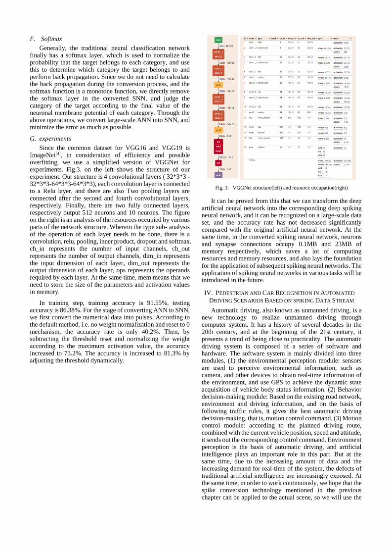
Since the common dataset for VGG16 and VGG19 is ImageNet[4], in consideration of efficiency and possible overfitting, we use a simplified version of VGGNet for experiments. Fig.3. on the left shows the structure of our experiment. Our structure is 4 convolutional layers ( 32*3*3 -32*3*3-64*3*3-64*3*3), each convolution layer is connected to a Relu layer, and there are also Two pooling layers are connected after the second and fourth convolutional layers, respectively. Finally, there are two fully connected layers, respectively output 512 neurons and 10 neurons. The figure on the right is an analysis of the resources occupied by various parts of the network structure. Wherein the type sub- analysis of the operation of each layer needs to be done, there is a convolution, relu, pooling, inner product, dropout and softmax. ch_in represents the number of input channels, ch_out represents the number of output channels, dim_in represents the input dimension of each layer, dim_out represents the output dimension of each layer, ops represents the operands required by each layer. At the same time, mem means that we need to store the size of the parameters and activation values in memory.

In training step, training accuracy is 91.55%, testing accuracy is 86.38%. For the stage of converting ANN to SNN, we first convert the numerical data into pulses. According to the default method, i.e. no weight normalization and reset to 0 mechanism, the accuracy rate is only 40.2%. Then, by subtracting the threshold reset and normalizing the weight according to the maximum activation value, the accuracy increased to 73.2%. The accuracy is increased to 81.3% by adjusting the threshold dynamically.

Fig. 3. VGGNet structure(left) and resource occupation(right)

It can be proved from this that we can transform the deep artificial neural network into the corresponding deep spiking neural network, and it can be recognized on a large-scale data set, and the accuracy rate has not decreased significantly compared with the original artificial neural network. At the same time, in the converted spiking neural network, neurons and synapse connections occupy 0.1MB and 23MB of memory respectively, which saves a lot of computing resources and memory resources, and also lays the foundation for the application of subsequent spiking neural networks. The application of spiking neural networks in various tasks will be introduced in the future.

IV. PEDESTRIAN AND CAR RECOGNITION IN AUTOMATED

DRIVING SCENARIOS BASED ON SPIKING DATA STREAM

Automatic driving, also known as unmanned driving, is a new technology to realize unmanned driving through computer system. It has a history of several decades in the 20th century, and at the beginning of the 21st century, it presents a trend of being close to practicality. The automatic driving system is composed of a series of software and hardware. The software system is mainly divided into three modules, (1) the environmental perception module: sensors are used to perceive environmental information, such as camera, and other devices to obtain real-time information of the environment, and use GPS to achieve the dynamic state acquisition of vehicle body status information. (2) Behavior decision-making module: Based on the existing road network, environment and driving information, and on the basis of following traffic rules, it gives the best automatic driving decision-making, that is, motion control command. (3) Motion control module: according to the planned driving route, combined with the current vehicle position, speed and attitude, it sends out the corresponding control command. Environment perception is the basis of automatic driving, and artificial intelligence plays an important role in this part. But at the same time, due to the increasing amount of data and the increasing demand for real-time of the system, the defects of traditional artificial intelligence are increasingly exposed. At the same time, in order to work continuously, we hope that the spike conversion technology mentioned in the previous chapter can be applied to the actual scene, so we will use the

spiking neural network instead of the traditional artificial intelligence neural network to deal with the perception module of automatic driving.

This part of the content aims to build a system that can quickly identify pedestrians and vehicles in the urban street scene as an auxiliary decision-making content of the automatic driving system. We adopt 2000 pictures from Cityscapes dataset[9] with weak annotation, in annotation with the presence/absence of a vehicle, with/without tagging a pedestrian.

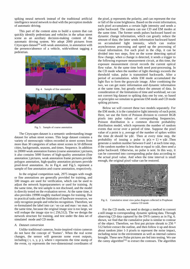
Fig. 4. Sample of fine annotation

Fig. 5. Sample of coarse annotation

The Cityscapes dataset is a semantic understanding image dataset for urban street scenes. This large dataset contains a variety of stereoscopic videos recorded in street scenes from more than 30 categories of urban street scenes in 50 different cities, backgrounds, seasons, and times. Sequence. In addition to 20000 weak annotation frames (coarse annotation ) pictures, it also contains 5000 frames of high-quality annotation (fine annotation ) pictures, weak annotation frame pictures provide polygon annotation, high-quality annotation pictures provide pixel-level annotation. As in Fig.4. and Fig.5. represent a sample of fine annotation and coarse annotation, respectively.

In the original competition task, 2975 images with rough or fine annotations are generally provided for training, and 500 images are used for verification, which can be used to adjust the network hyperparameters or used for training. At the same time, the test sample is not disclosed, and the model is directly tested on the evaluation server. At the same time, it also provides 19998 roughly marked images for training. Due to practical tasks and the limitation of hardware resources, we only recognize people and vehicles recognition. Therefore, we re-formulated the label into car / no car and man / no man. At the same time, because the original image size is too large, we will reshape the image size to ( 256,512). The we design the network structure for training, and test under the data set of simulated mode and CD mode.

A. Dataset conversion

Unlike traditional cameras, brain-inspired vision cameras do not have the concept of "frames". When the real scene changes, the sensor will generate some event outputs, including ( t, x, y, p ), where t represents the time stamp of the event, xy represents the two-dimensional coordinates of

the pixel, p represents the polarity, and can represent the rise or fall of the scene brightness. Based on the event information, each pixel accumulates a certain light intensity and sends a pulse backward. The camera can use CD and EM modes at the same time. The former sends pulses backward based on dynamic change information, which can greatly reduce the amount of data; the latter sends information backward based on accumulated light intensity, which can realize asynchronous processing and speed up the processing of visual information. For each pixel in the chip, it can be divided into two steps, first on the scene detecting optical flow change, when a change is detected, it sends a trigger to the following exposure measurement circuit, at this time, the exposure measurement circuit records the current optical flow value. At the same time both need post-processing. In the CD mode when the number of light rheology exceeds the threshold value, pulse is transmitted backwards. After a period of accumulation. while EM mode accumulated the light flux to form the grayscale image. After combining the two, we can get static information and dynamic information at the same time, but greatly reduce the amount of data. In consideration of the limitations of time and workload, we can not convert big dataset to spiking data one by one, so based on principles we simulate to generate EM mode and CD mode spiking pictures.

Below we will convert these two models separately. For the EM mode, it is the cumulative light intensity of each point. Here, we use the form of Poisson division to convert RGB pixels into pulse values of corresponding frequencies. Poisson distribution is a common discrete probability distribution model, which represents the number of random events that occur over a period of time. Suppose the pixel value of a point is γ, average of the number of spikes within the time ∆t should be γ∆t . Then at every time step, the probability of issuing a pulse is p(x = 1) ≈ γ∆t .Then generate a random number between 0 and 1 at each time step, if the random number is less than or equal to γ∆t, then send a pulse backward. Otherwise, no pulse is sent. In this way, it can be converted into corresponding pulse data according to the actual pixel value. And when the time interval is small enough, the original pixel value can be restored.

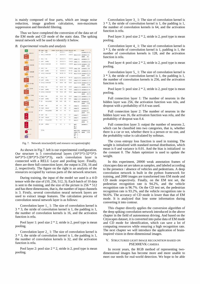
Fig. 6. Cumulative street view pulse diagram collected in Prophesee

camera CD mode

For the CD mode, we need to design a method to convert a still image to corresponding dynamic spiking data. Through observing CD data captured by the DVS camera as in Fig. 6. shown, we find that the cumulative pulse is similar to contour of the object. Therefore, we first put picture shrunk to 256 * 512 before extract the outline, and then follow it up and down about random jitter 1-3 pixels to represent the noise impact, including noise in the environment as well as internal camera brought. These new Pulse pictures are fed into testing. We use the canny algorithm[10] to extract the contours. The algorithm

is mainly composed of four parts, which are image noise reduction, image gradient calculation, non-maximum suppression and threshold filtering.

Thus we have completed the conversion of the data set of the EM mode and CD mode of the static data. The spiking neural network will be used to identify it below.

B. Experimental results and analysis

Fig. 7. Network structure(left) and resource occupation(right)

As shown in Fig.7. left is our experimental configuration. Our structure is 5 convolutional layers (16*3*3-32*3*3-64*3*3-128*3*3-256*3*3), each convolution layer is connected with a RELU Layer and pooling layer. Finally, there are three full connection layer, the output is 256, 16 and 2, respectively. The figure on the right is an analysis of the resources occupied by various parts of the network structure.

During training, the input of the model we used is a 4-D tensor with the size of (10, 256, 512, 3). Each batch of 10 data is sent to the training, and the size of the picture is 256 * 512 and has three dimensions, that is, the number of input channels is 3. Firstly, several convolution neural network layers are used to extract image features. The calculation process of convolution neural network layer is as follows:

Convolution layer 1_ 1: The size of convolution kernel is 3 * 3, the stride of convolution kernel is 1, the padding is 1, the number of convolution kernels is 16, and the activation function is relu.

Pool layer 1: pool size 2 * 2, stride is 2, pool type is mean pooling.





Convolution layer 4_ 1: The size of convolution kernel is 3 * 3, the stride of convolution kernel is 1, padding is 1, the number of convolution kernels is 128, and the activation function is relu.




Full connection layer 1: The number of neurons in the hidden layer was 256, the activation function was relu, and dropout with a probability of 0.4 was used.

Full connection layer 2: The number of neurons in the hidden layer was 16, the activation function was relu, and the probability of dropout was 0.4.

Full connection layer 3: output the number of neurons 2, which can be classified into two categories, that is, whether there is a car or not, whether there is a person or no one, and the probability value is calculated by softmax.

The cross entropy loss function is used in training. The weight is initialized with standard normal distribution, which mean is 0 and variance is 0.01. And the bias is initialized to the constant 0. The Adam optimizer is used to update the weight.

In this experiment, 20000 weak annotation frames of cityscapes data set are taken as samples, and labeled according to the presence / absence of vehicles and pedestrians. A deep convolution network is built in the python framework for training, and 2000 images are transformed into EM mode and CD mode respectively. Finally, on the EM test set, the pedestrian recognition rate is 94.2%, and the vehicle recognition rate is 96.7%. On the CD test set, the pedestrian recognition rate is 93.2%, and the vehicle recognition rate is 94.6%. The accuracy of CD mode is lower than that of EM mode. It is analyzed that lose some information during converting it into contour.

This chapter directly applies the conversion algorithm of the deep spiking convolution network introduced in the above chapter in the field of autonomous driving. And based on the Cityscapes dataset, it is converted into pulse data of EM mode and CD mode for identification, which can save a lot of computing resources while ensuring a high recognition rate. The next chapter we will introduce the application of brain-inspired vision in three-dimensional images.

V. STRUCTURED LIGHT IMAGE RECOGNITION BASED ON

PSE300EVK CAMERA

In recent years, the RGB method of representing two-dimensional images has become more and more unable to meet our needs for real-world detection. We hope to be able

to perceive the three-dimensional world, and this requires us to extract another one based on RGB information, that is, depth. For a solid object, as long as we can extract the RGB-D information of the object combined with surface information such as surface friction, we can model this object. Based on this, we found that the depth information that should be extracted is a weighted two-dimensional image, that is, each pixel should have a corresponding weight. This image is called a depth image.

Common three-dimensional modeling methods are binocular modeling, Time of Flight(ToF), structured light, etc. Because of its easy implementation and wide application, structured light has a far-reaching application in the new generation of payment level identification.

Because of its high recognition rate, prophesee camera can quickly get the depth information by encoding the structured light in time domain. We first use the Prophesee camera to complete a three-dimensional modeling system.

A. System configuration

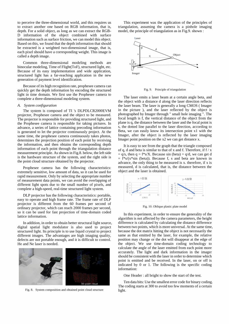
The system is composed of TI 's DLPDLCR2000EVM projector, Prophesee camera and the object to be measured. The projector is responsible for providing structured light, and the Prophesee camera is responsible for taking pictures. In advance, a series of lattice containing precoding information is generated to let the projector continuously project. At the same time, the prophesee camera continuously takes photos, determines the projection position of each point by receiving the information, and then obtains the corresponding depth information of each point through the triangulation distance measurement principle. As shown in Fig.8. below, the left side is the hardware structure of the system, and the right side is the point cloud structure obtained by the projector.

Prophesee camera has the following characteristics: extremely sensitive, low amount of data, so it can be used for rapid measurement. Only by selecting the appropriate number of measurement data points, we can avoid the overlapping of different light spots due to the small number of pixels, and complete a high-speed, real-time structured light system.

DLP projector has the following characteristics: portable, easy to operate and high frame rate. The frame rate of DLP projector is different from the 60 frames per second of ordinary projector, which can reach 2000 frames per second, so it can be used for fast projection of time-domain coded lattice information.

In addition, in order to obtain better structural light source, digital spatial light modulator is also used to project structured light. Its principle is to use liquid crystal to project different images. The advantages are high imaging quality, defects are not portable enough, and it is difficult to control. He and Ne laser is needed.

Fig. 8. System composition and obtained point cloud structure

This experiment was the application of the principles of triangulation, assuming the camera is a pinhole imaging model, the principle of triangulation as in Fig.9. shown :

Fig. 9. Principle of triangulation

The laser emits a laser beam at a certain angle beta, and the object with a distance d along the laser direction reflects the laser beam. The laser is generally a long CMOS ( Imager in the picture ), and the laser reflected by the object is photographed by Imager through " small hole imaging ". The focal length is f, the vertical distance of the object from the plane is q, the distance between the laser and the focal point is s, the dotted line parallel to the laser direction, according to Beta, we can easily know its intersection point x1 with the Imager, after the object is reflected by the laser imaging Imager point position on the x2 we can get distance x.

It is easy to see from the graph that the triangle composed of q, d and beta is similar to that of x and f. Therefore, if f / x = q/s, then q = f*s/X. Because sin (beta) = q/d, we can get d = f*s/(x*sin (beta)). Because f, s and beta are known in advance, the only thing to be measured is x. therefore, if x is measured, d is calculated, that is, the distance between the object and the laser is obtained.

Fig. 10. Oblique plastic plate model

In this experiment, in order to ensure the generality of the algorithm is not affected by the camera parameters, the height difference is calculated by calculating the distance difference between two points, which is more universal. At the same time, because the dot matrix hitting the object is not necessarily the same as that emitted by the laser, for example, the relative position may change or the dot will disappear at the edge of the object. We use time-domain coding technology to calculate the angle of the laser emitted from each point more accurately. The light and dark information in the imager should be consistent with the laser in order to determine which point is emitted and be received. In the laser, on or off is indicated by 0 or 1. The following is the specific coding information:

One Header : all bright to show the start of the test.

Ten data bits: Use the smallest error code for binary coding. The coding starts at 300 to avoid too few moments of a certain light.

Eight check digits: use CRC8 to check.

One tail: the light and dark intervals of the dot matrix to indicate the end of the test.

Then decode to know the position of each point, and use the check digit to determine the correctness.

Using this system, we obtained a depth model of an oblique plastic plate. The x-h and y-h images are shown in the Fig.10.:

Ideally, the two should be directly proportional to each other. From the experimental results, we noticed that the relative height difference shifted to the right rear side, presumably due to the shift of focus, and the small aperture imaging model was no longer established. Therefore, our subsequent experiments need to be carried out under stable conditions.

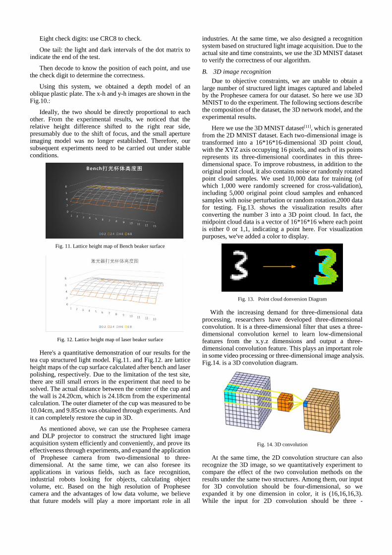
Fig. 11. Lattice height map of Bench beaker surface

Fig. 12. Lattice height map of laser beaker surface

Here's a quantitative demonstration of our results for the tea cup structured light model. Fig.11. and Fig.12. are lattice height maps of the cup surface calculated after bench and laser polishing, respectively. Due to the limitation of the test site, there are still small errors in the experiment that need to be solved. The actual distance between the center of the cup and the wall is 24.20cm, which is 24.18cm from the experimental calculation. The outer diameter of the cup was measured to be 10.04cm, and 9.85cm was obtained through experiments. And it can completely restore the cup in 3D.

As mentioned above, we can use the Prophesee camera and DLP projector to construct the structured light image acquisition system efficiently and conveniently, and prove its effectiveness through experiments, and expand the application of Prophesee camera from two-dimensional to three-dimensional. At the same time, we can also foresee its applications in various fields, such as face recognition, industrial robots looking for objects, calculating object volume, etc. Based on the high resolution of Prophesee camera and the advantages of low data volume, we believe that future models will play a more important role in all

industries. At the same time, we also designed a recognition system based on structured light image acquisition. Due to the actual site and time constraints, we use the 3D MNIST dataset to verify the correctness of our algorithm.

B. 3D image recognition

Due to objective constraints, we are unable to obtain a large number of structured light images captured and labeled by the Prophesee camera for our dataset. So here we use 3D MNIST to do the experiment. The following sections describe the composition of the dataset, the 3D network model, and the experimental results.

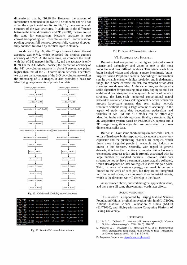
Here we use the 3D MNIST dataset[11], which is generated from the 2D MNIST dataset. Each two-dimensional image is transformed into a 16*16*16-dimensional 3D point cloud, with the XYZ axis occupying 16 pixels, and each of its points represents its three-dimensional coordinates in this three-dimensional space. To improve robustness, in addition to the original point cloud, it also contains noise or randomly rotated point cloud samples. We used 10,000 data for training (of which 1,000 were randomly screened for cross-validation), including 5,000 original point cloud samples and enhanced samples with noise perturbation or random rotation.2000 data for testing. Fig.13. shows the visualization results after converting the number 3 into a 3D point cloud. In fact, the midpoint cloud data is a vector of 16*16*16 where each point is either 0 or 1,1, indicating a point here. For visualization purposes, we've added a color to display.

Fig. 13. Point cloud donversion Diagram

With the increasing demand for three-dimensional data processing, researchers have developed three-dimensional convolution. It is a three-dimensional filter that uses a three-dimensional convolution kernel to learn low-dimensional features from the x.y.z dimensions and output a three-dimensional convolution feature. This plays an important role in some video processing or three-dimensional image analysis. Fig.14. is a 3D convolution diagram.

Fig. 14. 3D convolution

At the same time, the 2D convolution structure can also recognize the 3D image, so we quantitatively experiment to compare the effect of the two convolution methods on the results under the same two structures. Among them, our input for 3D convolution should be four-dimensional, so we expanded it by one dimension in color, it is (16,16,16,3). While the input for 2D convolution should be three -

dimensional, that is, (16,16,16). However, the amount of information contained in the two will be the same and will not affect the experimental results. As Fig.15., there are network structure of the two structures. In addition to the difference between the input dimensions and 2D and 3D, the two are set the same for comparison. Network structure is two convolution-pooling-two convolution-batch normalization- pooling-dropout-full connect-dropout-fully connect-dropout- fully connect, followed by softmax layer to classify.

As shown in Fig. 16., after 20 epochs were trained, the test accuracy was 0.742, which exceeded the original author's accuracy of 0.7275.At the same time, we compare the result with that of 2-D network in Fig. 17., and the accuracy is only 0.694.On the 3-D MNIST dataset, the prediction accuracy of the 3-D convolution network is about 5 percentage points higher than that of the 2-D convolution network. Therefore, we can see the advantages of the 3-D convolution network in the processing of 3-D images. It also provides a basis for identifying large amounts of point cloud data.

Fig. 15. 3D(left) and 2D(right) network structres

Fig. 16. Result of 3D convolution network

Fig. 17. Result of 2D convolution network

VI. SUMMARY AND PROSPECT

Brain-inspired computing is the highest point of current science and technology, and vision is one of the most important and most difficult modules. This article starts from brain-inspired vision and adopts a more biomimetic brain-inspired vision Prophesee camera. According to information sent its dynamic event, with high resolution and high dynamic range, for in some exercise too fast, too exposed or too dark scene to provide new idea. At the same time, we designed a spike algorithm for processing pulse data, hoping to build an end-to-end brain-inspired vision system. In terms of network structure, the large-scale numerical convolutional neural network is converted into a spiking neural network, which can process large-scale general data sets, saving network resources without losing a large amount of accuracy; In the aspect of static pulse data recognition, pedestrians and vehicles in two EM and CD modes can be effectively identified in the auto-driving scene; finally, a structured light 3D acquisition system based on PSE300EVK camera and a 3D image recognition algorithm are constructed for three-dimensional spike data.

But we still have some shortcomings in our work. First, in terms of hardware, brain-inspired visual cameras are now very expensive and the purchasing channels are complex, which limits more insightful people in academia and industry to invest in this research. Secondly, with regard to generic datasets, it is true that traditional computer vision has made tremendous progress today and is strongly associated with its large number of standard datasets. However, spike data streams do not yet have a common dataset actually collected, which also depends on later colleagues to solve this pain point. Third, in terms of system synergy, our work is currently limited to the work of each part, but they are not integrated into the actual scene, such as medical or industrial robots, which is the direction we will develop in the future.

As mentioned above, our work has great application value, and there are still some shortcomings worth later efforts.

ACKNOWLEDGMENT

This research is supported by Beijing Natural Science Foundation Haidian original innovation joint fund (L172009), National Natural Science Foundation of China (NSFC) (61471010), and High-performance Computing Platform of Peking University.

REFERENCES

[1] Liu S C，Delbruck T．Neuromorphic sensory systems[J]. “Current Opinion in Neurobiology"，2010，20( 3) : 288-295．

[2] Mahar M A C，DeWeerth S P，Mahowald M A，et al．Implementing neural architectures using analog VLSI circuits[J]. IEEE Transactions on Circuits Systems, 1989，36 ( 5 ) : 643-652．

[3] Prophesee Corperation, https://www.prophesee.ai/.

https://www.prophesee.ai/

[4] LeCun, B.Boser, J.S.Denker, D.Henderson, R.E.Howard, W.Hubbard, and L.D.Jackel. Backpropagation applied to handwritten zip code recognition. Neural Computation, 1989.

[5] Akira Hasegawa, Kazuyoshi Itoh, Yoshiki Ichioka. Generalization of shift invariant neural networks: Image processing of corneal endothelium[J]. Neural Networks, 1996, 9(2):345-356.

[6] Maas W. Networks of spiking neurons: the third generation of neural network models[J]. Neural Networks, 1997, 14(4): 1659-1671.

[7] Simonyan K , Zisserman A . Very Deep Convolutional Networks for Large-Scale Image Recognition[J]. Computer Science, 2014.

[8] Krizhevsky, Alex & Sutskever, Ilya & Hinton, Geoffrey. ImageNet Classification with Deep Convolutional Neural Networks[J]. Neural Information Processing Systems. 2012, 25.

[9] M. Cordts, M. Omran, S. Ramos, T. Rehfeld, M. Enzweiler, R. Benenson, U. Franke, S. Roth, and B. Schiele, The Cityscapes Dataset for Semantic Urban Scene Understanding[C]. IEEE Conference on Computer Vision and Pattern Recognition (CVPR), 2016.

[10] Canny, J., A Computational Approach To Edge Detection, IEEE Transactions on Pattern Analysis and Machine Intelligence, 1986, 8(6):679–698.

[11] 3D MNIST, https://www.kaggle.com/daavoo/3d-mnist

Research on Brain-inspired Vision Based on Dynamic Vision ...

Documents

Transcript of Research on Brain-inspired Vision Based on Dynamic Vision ...