
research for RIJKSINSTITUUT VOOR VOLKSGEZONDHEID EN … · 2001-07-13 · research for man and...
194
research for man and environment RIJKSINSTITUUT VOOR VOLKSGEZONDHEID EN MILIEU NATIONAL INSTITUTE OF PUBLIC HEALTH AND THE ENVIRONMENT RIVM report 481505 024 Valuing the benefits of environmental policy: The Netherlands A. Howarth, D.W. Pearce, E. Ozdemiroglu, T. Seccombe-Hett a) K. Wieringa, C.M. Streefkerk, A.E.M. de Hollander March 2001 This investigation has been performed by order and for the account of the Ministry of Economic Affairs: the Netherlands, within the framework of project 481505, European Environmental Priorities. a) EFTEC, 16 Percy Street, London, W1P 9FD, UK. RIVM, P.O. Box 1, 3720 BA Bilthoven, telephone: 31 - 30 - 274 91 11; telefax: 31 - 30 - 274 29 71
Transcript of research for RIJKSINSTITUUT VOOR VOLKSGEZONDHEID EN … · 2001-07-13 · research for man and...

research forman and environment
RIJKSINSTITUUT VOOR VOLKSGEZONDHEID EN MILIEUNATIONAL INSTITUTE OF PUBLIC HEALTH AND THE ENVIRONMENT
RIVM report 481505 024
Valuing the benefits of environmental policy:The NetherlandsA. Howarth, D.W. Pearce, E. Ozdemiroglu, T.Seccombe-Hetta)
K. Wieringa, C.M. Streefkerk, A.E.M. deHollander
March 2001
This investigation has been performed by order and for the account of the Ministry ofEconomic Affairs: the Netherlands, within the framework of project 481505, EuropeanEnvironmental Priorities.
a)EFTEC, 16 Percy Street, London, W1P 9FD, UK.
RIVM, P.O. Box 1, 3720 BA Bilthoven, telephone: 31 - 30 - 274 91 11; telefax: 31 - 30 - 274 29 71
page 2 of 194 EFTEC/RIVM report 481505 024
Abstract
This study seeks to set priorities for environmental policy in the Netherlands. The report focuses onseven environmental issues including: climate change, acidification, low level ozone, particulatematter, noise, eutrophication and land contamination. These issues are prioritised using three differentapproaches: damage assessment, public opinion and ‘disability adjusted life years’(DALYs).
The damage assessment approach largely follows that of the European Commission DG Environmentstudy ‘European Environmental Priorities: an integrated economic and environmental assessment’(RIVM et al, forthcoming 2001). It is based on a logical stepwise progression through emission,change in exposure, quantification of impacts using exposure-response functions, to valuation basedon willingness to pay. The existence of significant uncertainty in assessment of environmentaldamage is dealt with by conducting a transparent sensitivity analysis for each issue, this demonstratesthe consequences of uncertainty on the robustness of our conclusions. The public opinion approachmakes use of European and national surveys to determine the importance of environmental issues asperceived by the population of the Netherlands. The DALY methodology largely follows that ofMurray and Lopez (1996). This procedure combines years of life lost and years lived with disease ordisability that are weighted according to severity.
According to the damage assessment approach the priorities, in terms of potential benefits from fullcontrol, are low level ozone, land contamination and particulate matter, followed by acidification andclimate change, whilst noise and eutrophication are estimated to yield the lowest potential benefitsfrom control. However, in the absence of cost estimates no conclusions can be reached on thedesirability of control measures. Public opinion surveys show that environmental issues other than theseven considered in this study are a major concern for the Dutch public, namely chemical release andoil pollution. However, focusing on the seven issues considered in this study, the Dutch public rank,climate change, acidification, eutrophication and air pollution from cars (interpreted as low-levelozone and PM10) as the issues of most concern. According to the DALYs approach the health effectsof air pollution from particulate matter, and to a certain degree from low level ozone, dominate thedisease burden. The future disease burden is largely due to changes in the population structure, i.e. anincreasing, aged population. Another environmental problem associated with a high disease burden isnoise exposure from road and air traffic.
Based on a simple ‘Borda count’, a final ranking for the environmental issues is made. This studyconcludes that land contamination, climate change and particulate matter are top priorityenvironmental issues in the Netherlands, followed by acidification, low level ozone, eutrophicationand finally noise. These findings suggest that future policies focusing on the top issues may yieldconsiderable benefit depending on their cost of control.Although ranking environmental issues is useful in the sense of highlighting priority issues andindicating if there is any surprise environmental issues for the Netherlands. It is important to note thatthe benefit estimates offer only some guidance on environmental priorities, in the absence of data oncosts of implementing policies only part of the picture necessary for establishing priorities isprovided. For a full-scale economic analysis benefit estimates need to be compared with costestimates within a CBA framework. This is outside the scope of this study, however a separate paperon the issues relating to and experience with such CBAs is presented in Annex II.

EFTEC/RIVM report 481505 024 page 3 of 194
Preface
This study has been written by a multi-disciplinary team composed of environmental economists fromEconomics for the Environment (EFTEC) and scientist, economists and modellers at NationalInstitute of Public Health and the Environment (RIVM) for the Ministry of Economic Affairs, theNetherlands, in May 2000. The Ministry of Economic Affairs’ aim, to further examine the potentialbenefit estimates as a guiding tool in environmental policy, was the basis for commissioning thisstudy. The main report is an assessment of the environmental damage due to seven environmentalissues in the Netherlands. Damage estimates can be interpreted as benefit estimates of environmentalcontrol and can be used as a tool to facilitate an environmental priority scheme for the Netherlands.Annex II presents a paper, written by Professor David Pearce, that examines the role of cost-benefitanalysis in efficient decision-making.
The assessment in the main report is new and refreshing for the Netherlands and indeed improvesunderstanding of the potential of benefit estimates as a guiding tool in environmental policy.
Bilthoven, March 2001.

page 4 of 194 EFTEC/RIVM report 481505 024
EFTEC/RIVM report 481505 024 page 5 of 194
Contents
Samenvatting 9
Summary 16
1. Background to and scope of the study 23
2. Structure of the report 25
3. Methodology for setting priorities in environmental policy 27
3.1 Introduction 27
3.2 Overview of methodologies for setting priorities in environmental policy 27
3.3 Monetary damage estimation methodology 28
3.4 Public opinion methodology 35
3.5 Disability adjusted life years’ (DALYs) 36
4. Application of damage assessment methodology 37
4.1 Climate change 384.1.1 The issue 384.1.2 Source of emissions 384.1.3 Physical measure of impacts 384.1.4 Monetary measure of impact 404.1.5 Aggregate monetary damage estimate 464.1.6 Uncertainty 48
4.2 Acidification 534.2.1 The issue 534.2.2 Source of emissions 534.2.3 Physical measure of impacts 534.2.4 Monetary measure of impact 554.2.5 Aggregate monetary damage estimate 574.2.6 Uncertainty 58
4.3 Noise 654.3.1 The issue 654.3.2 Source of emissions 654.3.3 Physical measure of impacts 654.3.4 Monetary measure of impacts 674.3.5 Aggregate monetary damage estimate 714.3.6 Uncertainty 77
4.4 Land contamination 804.4.1 The issue 804.4.2 Source of emissions 804.4.3 Physical measure of impacts 804.4.4 Aggregate monetary damage estimate 814.4.5 Uncertainty 83
4.5 Particulate matter 854.5.1 The issue 854.5.2 Source of emissions 854.5.3 Physical measure of impacts 85

page 6 of 194 EFTEC/RIVM report 481505 024
4.5.4 Monetary measure of impact 864.5.5 Uncertainty 87
4.6 Eutrophication 904.6.1 The issue 904.6.2 Source of emissions 904.6.3 Physical measure of impacts 904.6.4 Monetary measure of impacts 914.6.5 Aggregate monetary damage estimate 944.6.6 Uncertainty 94
4.7 Low level ozone 964.7.1 The Issue 964.7.2 Source of emissions 964.7.3 Physical measure of impacts 964.7.4 Monetary measure of impacts 984.7.5 Aggregate monetary damage estimate 994.7.6 Uncertainty 100
4.8 Damage assessment and priority issues 1074.8.1 Ranking environmental issues according to damage estimates 1074.8.2 Burden of disease associated with selected environmental exposures 109
5. Public opinion in the Netherlands 115
5.1 Environmental issues in general 115
5.2 Global environmental issues 115
5.3 National environmental issues 116
5.4 Attitudes towards the future 117
5.5 Environmental protection action- who is responsible? 117
6. Prioritisation of environmental issues 119
References 123
Annex I Methodology and assumptions 133
1. Monetary valuation techniques 133
2. Benefits transfer 139
3. Valuing the risk of premature mortality 143
4. Monetary valuation of morbidity effects 149
5. Environmental data, assumptions and models 151
6. Data flows of the 5th National Environmental Outlook 159
Annex II Integrating cost-benefit analysis into the policy process 163
1. Purpose of the paper 165
2. The issue: how to introduce rationality in public decision-making 166
3. The criteria / alternatives matrix 169
4. Summary so far 170
5. What if all costs and benefits cannot be monetised? 170
6. The issue of geographical bounds 171

EFTEC/RIVM report 481505 024 page 7 of 194
7. Experience with CBA 172
8. Obstacles to the use of Cost-Benefit Analysis 175
9. Baseline 176
10. Obstacles: credibility 178
11. Obstacles: moral objections to Cost-Benefit Analysis and the issue of democracy 180
12. Obstacles: the efficiency focus of Cost-Benefit Analysis 182
13. Obstacles: flexibility of process 183
14. Obstacles: is Cost-Benefit Analysis non-participatory? 183
15. Obstacles: capacity 184
16. Getting Cost-Benefit Analysis into the process of decision-making 184
Appendix A Types of formal appraisal procedures 187
Mailing list 193

page 8 of 194 EFTEC/RIVM report 481505 024
Abbreviations∆ Change inAOT40 Accumulated ozone above threshold 40ppb, (usually for crops)AOT60 Accumulated ozone above threshold 60ppb, (usually for health)BT Benefits transferCBA Cost benefit analysisCLS Current legislation scenarioCO Carbon monoxideCO2 Carbon dioxideCOI Cost of illnessCOPD Chronic obstructive pulmonary diseaseCVM Contingent valuation methodologyDALY Disability adjusted life yearsdB(A) Decibel exposure level of noiseD/ERF Dose / exposure response functionsEU European UnionGDP Global damage potentialGDP Gross domestic productGNP Gross national productGHG Greenhouse gasesGWP Global warming potentialIPCC Intergovernmental Panel on Climate ChangeMWTP Marginal willingness to payN Nitrogenn NoiseN2O Nitrous oxideNH3 AmmoniaNO2 Nitrogen dioxideNOx Oxides of nitrogenNEO5 Fifth National Environmental Outlook (draft report) (final July 2000)NSDI Noise sensitivity depreciation indexO3 Low level ozone, otherwise known as tropospheric ozoneP Phosphorousp.a. Per annumPB Primary benefitPM10 Fine particles less than 10µm in diameterPM2.5 Fine particles less than 2.5µm in diameterPOP Populationpp Per personppb parts per billionPPP Purchasing power parityRAD Restricted activity dayRHA Respiratory hospital admissionSO2 Sulphur dioxideUNECE United Nations Economic Commission for EuropeVOCs Volatile organic compoundsVOLY Value of life yearVOR Value of riskVOSL Value of statistical lifeWTP Willingness to payY Income

EFTEC/RIVM report 481505 024 page 9 of 194
SamenvattingAchtergrondHet doel van deze studie is het stellen van mogelijke prioriteiten voor het Nederlands milieubeleid. Destudie is uitgevoerd door het Economics for the Environment Consultancy (EFTEC) in samenwerkingmet het Rijksinstituut voor Volksgezondheid en Milieu (RIVM) in opdracht van het Ministerie vanEconomische Zaken.
Het rapport beschrijft drie verschillende methoden om prioriteiten te stellen binnen het milieubeleid:• Schadeschatting voor de huidige status van zeven milieuproblemen (1995) en de verwachtte
toekomstige ontwikkeling (2010, 2020 en 2030). Schadeschattingen geven een indicatie voor depotentiële baten van milieumaatregelen, met andere woorden de voorkomen schade is gelijk aande baten van milieumaatregelen;
• Publieke opinie als maatstaf voor het belang van milieuproblemen, zoals waargenomen bij deNederlandse bevolking, en
• ‘Disability adjusted life years’ (DALY’s).
MilieuproblemenHet rapport richt zich op zeven milieuproblemen. Deze problemen zijn:• Klimaatverandering;• Verzuring;• Troposferische ozon;• Fijn stof;• Geluid;• Eutrofiëring, en• Bodemverontreiniging.
Deze onderwerpen zijn tot prioriteit verkozen door de stuurgroep om twee hoofdredenen:i) Momenteel is het beleid voor deze onderwerpen of niet op zijn plaats of niet geheel effectief1,
enii) De verwachting is dat de geselecteerde onderwerpen in Nederland in belang zullen toenemen
in de komende decennia.
De data zijn afkomstig uit de concept versie van de Nederlandse Nationale Milieuverkenning 5(definitieve versie beschikbaar augustus 2000). Er is gekozen voor het ‘EC’ scenario, wat hier wordtaangeduid met ‘current legislation scenario’ (CLS). De toekomstige ontwikkelingen van demilieuproblemen zijn gebaseerd op maatschappelijke trends gecombineerd met het huidigemilieubeleid, zoals het reeds vastgesteld is in Nederland en de EU. Tabel 1 geeft de aannames die tengrondslag liggen aan het CLS.
1 De stuurgroep heeft besloten om bodemverontreiniging in de studie op te nemen ondanks het huidige beleiddat bodemverontreiniging beperkt. Dit is gedaan om te kijken wat de prioriteit van bodemverontreiniging is invergelijking met de andere milieuproblemen.

page 10 of 194 EFTEC/RIVM report 481505 024
Tabel 1 Maatschappelijke trends en milieubeleid in het CLSMaatschappelijke trends• Opkomst van ‘Fortress America’ en de trend dat strategische handel en industrieel beleid
significant bijdragen aan het vormen van handelsblokken;• Ondanks toenemende gespannen relaties met de USA ontwikkelt West-Europa zich erg
gunstig. Het Europese proces van integratie is een belangrijke stimulans voor eenversterking van de structuur van het West-Europese produkt en arbeidsmarkt. Eenverreikend proces van hervorming van de West Europese welvaartsstaat wordt inbeweging gezet. Hierin worden pogingen gedaan om de Europese traditie van socialegelijkheid te combineren met een toegenomen gevoeligheid voor economischestimulansen;
• De EU introduceert een energieheffing van $ 10 per barrel;• Technologische ontwikkeling en verspreiding is gematigd;• Hoge migratie naar de EU.Belangrijk milieubeleid in het CLS*• Klimaatbeleid (1999); invoering van het Kyoto protocol;• Europese emissies instructies (e.g., EURO IV);• Meest recente normen voor emissie bij verbranding;• Geïntegreerd beleid voor de reductie van ammoniak en mest;• Meest recente geluidsnormen voor transport.* Beleid goedgekeurd door het Nederlands parlement voor 1 januari 2000
MethodenSchadebenaderingDe toegepaste methode komt grotendeels overeen met de methode die gevolgd is voor de studie‘European Environmental Priorities: an integrated economic and environmental assessment’ (RIVMet al., 2000)2 voor de Europese Commissie DG Milieu. De methode is gebaseerd op een logischestapsgewijze opeenvolging van emissies, verandering in blootstelling, kwantificeren van effecten metbehulp van blootstellings-effect relaties, tot waardering gebaseerd op ‘willingness-to-pay’ (WTP).
We onderkennen het bestaan van significante onzekerheid bij het schatten van milieuschade alsgevolg van:• Statistische fout;• Overbrengen van blootstellings-effect relaties en waarderingen naar een andere context (locatie en
tijd) ;• Variatie in politieke en ethische opvattingen, en• Tekortkomingen in het huidige kennisniveau, in sommige gevallen leidend tot het weglaten van
effecten.
We benaderen het bestaan van onzekerheid door het zoveel mogelijk kwantificeren van effecten,gebruikmakend van wat wij de beste beschikbare data vinden (na een uitgebreide bestudering van deliteratuur), en de aannames die zoveel mogelijk overeenkomen met deze data. Wij anticiperen op hetbestaan van onzekerheid door het uitvoeren van een gevoeligheidsanalyse om op een overzichtelijkemanier de gevolgen van de onzekerheid op de robuustheid van onze conclusies, gebaseerd op onzebaseline data en aannames, weer te geven. Om een duidelijk overzicht te bewaren is er eengevoeligheidsanalyse uitgevoerd voor elk milieuprobleem.
De belangrijkste bronnen van onzekerheid, zoals vastgesteld in loop van deze studie, zijn devolgende:
2 Met uitzondering van bodemverontreiniging, welke niet was opgenomen in deze studie. Voor een uitgebreideuiteenzetting van de ontwikkelde en gebruikte methode voor dit onderwerp, zie Section 4.4.

EFTEC/RIVM report 481505 024 page 11 of 194
• Benadering van de waardering van vroegtijdige sterfte;• De ‘willingness-to-pay’ waarden worden constant veronderstelt, in Euro 2000 waarden, over de
gehele tijdsperiode ondanks een stijgend Nederlands BBP.• De relatie tussen blootstelling en uiteindelijke gezondheidseffecten, oftewel de blootstellings-
effectrelaties;• Het beleid ter voorkoming van klimaatverandering kan hogere baten voortbrengen wanneer de
secundaire baten als gevolg van andere milieuproblemen worden meegenomen. Aan de anderekant kan de schade overschat worden door het weglaten van aanpassingsstrategieën;
• De baten van verzuring kunnen onderschat zijn door het weglaten van de effecten opecosystemen, cultuurgoederen en zichtbaarheid. De baten van verzuring kunnen overschatworden, doordat de effecten van PM10 op de volksgezondheid worden meegenomen, terwijl dezeeffecten al in de separate analyse voor PM10 berekend worden;
• De aanname voor geluidhinder is dat alle type geluid hetzelfde gewaardeerd worden, ondanks hetbewijs dat veronderstelt dat geluid van vliegtuigen en railverkeer als ‘erger’ beschouwd wordt dangeluid als gevolg van wegverkeer;
• De baten van bodemverontreiniging zijn behoorlijk onzeker als gevolg van de data met betrekkingtot het aantal verontreinigde locaties, het omzetten van aantal locaties in omvang verontreinigdegrond, en de waarde van schone / verontreinigde grond;
• De baten van fijn stof worden geschat op basis van de aanname dat alle fracties van PM10 evenschadelijk zijn voor de volksgezondheid en het feit dat in de resultaten andere ziekte-effecten danziekenhuisopnames niet zijn opgenomen;
• Eutrofiëring; aanzienlijke onzekerheid omtrent de wetenschappelijke data voor de waterkwaliteitin Nederland en het gebrek aan bewijs voor een WTP voor daling van de eutrofieringseffectenvoor binnenwateren in Nederland, en
• Troposferische ozon; niet meegenomen zijn de effecten op materialen, bosecosystemen, niet-gewas begroeiing en biodiversiteit, en de ziekte effecten anders dan ziekenhuisopnames.
Deze en andere bronnen zijn vollediger uiteengezet en onderzocht in het rapport.
Sommige criticie beweren dat het bestaan van onzekerheid de betrouwbaarheid van eenbatenschatting of de batenschatting als een beslissingsinstrument ondermijnt. Het is onzeprofessionele opvatting dat de aanwezigheid van een grote onzekerheid het essentiëler maakt om eenbatenschatting uit te voeren. Een batenschatting vergroot de kennis in het probleemgebied en het geeftpoliticie een indicatie voor het potentiële risico van hun acties. Een alternatieve benadering is datalleen de baten waarvan de begeleidende onzekerheid als minimaal gekwantificeerd is, wordenmeegenomen. Echter dit zou betekennen dat het noodzakelijk is om een subjectief standpunt in tenemen met betrekking tot hoe goed het bewijs moet zijn om een gegeven effect als robuust tebeschouwen voor de analyse. Behalve het vaststellen of een vervuiler schadelijk is, geeft het eengebrekkig advies voor de reeks van mogelijke effecten van de onderzochte vervuilers.
Publieke opiniebenaderingOm de belangrijkheid van de milieuproblemen zoals bezien door de Nederlands bevolking te bepalen,refereren we naar Europese en nationale onderzoeken. De redenen om naar publieke opinie te kijkenzijn tweeledig;• Verscheidene Europese en nationale onderzoeken tonen dat het milieu een belangrijke bron van
zorg blijft voor de Nederlandse bevolking, en• Het gebruik van publieke opinie voor het rangschikken van milieuproblemen verzekert dat alle
inwoners van Nederland een even hoge weging hebben. Met andere woorden, ze krijgen in feiteeen even groot aantal ‘stemmen’ over het milieu. Een dergelijke rangschikking vanmilieuproblemen is daarom ongevoelig voor verschil in factoren, die een batenschatting kunnenbeïnvloeden, zoals bijvoorbeeld inkomen.

page 12 of 194 EFTEC/RIVM report 481505 024
Disability adjusted life years (DALY’s) benaderingDe gebruikte methode komt grotendeels overeen met de methode van Murray en Lopez (1996). Zijontwikkelden de ‘disability adjusted life years’ maatstaf om de wereldwijde ziektelast en dedaaruitvolgende gezondheidsbeleidsprioriteiten in verschillende regio’s van de wereld te schatten.Deze gezondheidseffectmaatstaf combineert verlies van levensjaren en jaren geleefd met ziekte ofhandicap, die gewogen zijn naar zwaarte.
In het kader van de 5e Nationale Milieuverkenning zijn alleen adequate data en toekomstperspectievenbeschikbaar voor fijn stof, troposferische ozon, geluid, ultra-violette straling, radon, huisvochtigheiden ziekte als gevolg van voedselinfecties. Voor elke relevante gezondheidsuitkomst berekenen wetoegeschreven risico’s door het combineren van populatie gewogen blootstellingverdeling metrelatieve risicoschattingen, afgeleid uit de epidemiologische literatuur. Vervolgens is voor iederegezondheidsuitkomst het aantal gevallen geschat door het combineren van de in de baselinevoorkomende gevallen met de toegevoegde risico’s. Berekeningen van de toekomstige ziektelast zijngebaseerd op projecties van de toekomstige populatiestructuur. Wij presenteren de gebruikte set vaneindpunten om te komen tot de schattingen van toegeschreven ziektelast en het aantal verlorenDALY’s. Tenslotte is de totale blootstelling toegeschreven aan ziektelast berekend door hetaggregeren van het aantal DALY’s voor elke gezondheidsuitkomst. De ziektelast veroorzaakt dooradditionele UV-blootstelling, als gevolg van degradatie van de ozonlaag, is berekend door hetaggregeren van jaarlijkse ziekte en sterfte schattingen van huidkanker en de Nederlandse ziektelastdata, Melse et al (2000). Statistische onzekerheid is geschat met MonteCarlo technieken.
ResultatenSchadebenaderingOm voor de milieuproblemen op basis van schade (of potentiële baten van beleid) prioriteiten testellen, moeten de schatting direct vergelijkbaar gemaakt worden. Dit wordt gecompliceerd door hetfeit dat de schadeschattingen voor geluid en bodemverontreiniging contante waarden over eenoneindige periode zijn. Dus we vergelijken de milieuproblemen met de contante waarde van deschadeschatting (rente = 6%). In Tabel 2 worden de totale schadeschattingen gegeven als een nettocontante waarde en de overeenkomende waarde voor de jaarlijkse schade, vervolgens zijn deNederlandse milieuthema’s gerangschikt naar de hoogste potentiële baten van beleid.
Tabel 2 Totale en jaarlijkse schadeschattingen voor milieuthema’s in NederlandTotale schade
Netto contante waarderentevoet=6%
Miljoen Euro(2000)
Jaarlijkse schademiljoen Euro (2000)
Rangschikking
Troposferische ozon 110034 – 110613 6228 - 6261 1Bodemverontreiniging 59559 3371 2PM10 54471 3083 3Verzuring 37017 - 41569 2095 - 2353 4Klimaatverandering 36766 2081 5Geluid 31980 1810 6Eutrofiëring 9835 - 19224 557 - 1088 7
Dus we zien dat de hoogste prioriteit, in termen van potentiële baten van volledig beleid, ligt bijtroposferische ozon, bodemverontreiniging en fijn stof. Gevolgd door klimaatverandering enverzuring, terwijl voor geluid en eutrofiëring geschat wordt dat ze de laagste potentiële baten zullenopleveren. Maar er kunnen geen conclusies ten aanzien van de wenselijkheid van beleid getrokkenworden, omdat kostenschattingen ontbreken.
Ondanks dat de schade en dus de potentiële primaire baten van beleid voor milieuproblementoenemen in de tijd (met uitzondering van eutrofiëring en verzuring), dalen ze als percentage van hetNederlands BBP in 1995, 2010, 2020 and 2030. Tabel 3 geeft de schadeschattingen als percentage

EFTEC/RIVM report 481505 024 page 13 of 194
van het BBP. Aangemerkt moet worden dat dalende percentages van het BBP geen garantie gevenvoor een stijging van de relatieve waarde van het milieu in de tijd als het inkomen stijgt. Als derelatieve waarde met hetzelfde percentage stijgt als het BBP, dan blijft de schade als deel van het BBPgelijk. Maar er is slechts weinig informatie beschikbaar over de inkomenselasticiteit van de vraag naarmilieu, dus we nemen aan dat ‘willingness to pay’ (WTP) waarden constant blijven in de tijd ondankseen stijgend BBP voor Nederland.
Tabel 3 Milieuschadeschattingen als percentage van Nederlands BBP: %1995 2010 2020 2030
Troposferische ozon 1,32 1,12 1,01 1,02PM10 0,76 0,53 0,47 0,46Klimaatverandering 0,62 0,40 0,33 0,27Verzuring 0,85 – 0,95 0,30 – 0,34 0,23 – 0,25 0,18 – 0,20Eutrofiëring 0,22 – 0,45 0,08 – 0,16 0,06 – 0,12 0,05 – 0,09Geluid 0,51 0,38 0,30 0,25Totaal 4,29 – 4,62 2,82 – 2,92 2,40 – 2,48 2,22 – 2,29Nederlands BBP (miljard Euro): 1995 = 312,627; 2010 = 482,543; 2020 = 632,928; 2030 =830,180; bron RIVM(2000).
Tabel 3 suggereert dat milieuschade in Nederland een significant aandeel is van het BBP in 1995, eenspreiding van 1.3% voor tropsferische ozon, tussen 0.6% en 0.8% voor fijn stof, klimaatverandering,verzuring tot ruwweg 0.5% voor geluid en eutrofiëring. In totaal is de milieuschade als gevolg vanbovenstaande milieuproblemen geschat op ruwweg 4.5% van het BBP in 1995, dalend tot ongeveer2% in 2030. Het is interessant om deze getallen te vergelijken met de schattingen voor uitgaven aanvervuilingbestrijding, waarvan aangegeven is dat ze ongeveer 1.2% van het BBP in 1990 zijn(ERECO, 1992).
Publieke opiniebenaderingOndanks dat het milieu minder als een probleem wordt gezien in 1999 dan in 1995, wanneer debezorgdheid op haar hoogtepunt was, (63% in 1986, 80% in 1995 en 70% in 1999), (Eurobarometer1986, 1995 en 1999), blijft het een punt van gemeenschappelijke zorg voor het Nederlandse publiek.Tabel 4 laat de onderwerpen zien die serieuze bedreiging voor het milieu vormen (ongeacht deschaal), zoals waargenomen bij het Nederlands publiek.
Deze opinies zijn tamelijk stabiel in de tijd en de resultaten van 1992 geven eenzelfde beeld (behalvehet onderwerp zure regen, dat iets belangrijker geworden is sinds 1992).
Tabel 4 Onderwerpen die bijdragen aan serieuze milieuschade: 1992 and 1995Onderwerp RangschikkingFabrieken die gevaarlijke chemicaliën uitstoten in lucht en water 1Olievervuiling van zeeën en kusten 2Wereldwijde vervuiling (geleidelijke verdwijning van tropisch regenwoud,afbraak van de ozonlaag, broeikaseffect etc)
3
Opslag van radioactief afval 4Industrieel afval 5Zure regen 6Overmatig gebruik van herbiciden, insecticiden en kunstmest in de landbouw 7Zwerfvuil op straat, in groene gebieden of op het strand 8Luchtverontreiniging door auto’s 9Ongecontroleerd massa toerisme 10Afvalwater 11Geluid ontstaan door openbare gebouwen of werken, zwaar verkeer, luchthavens 12Bron: Eurobarometer: Europeans and their Environment, 1992, 1995 en SCP onderzoek 1993.

page 14 of 194 EFTEC/RIVM report 481505 024
Disability adjusted life years (DALY’s) benaderingDe gezondheidseffecten van luchtverontreiniging door fijn stof en gedeeltelijk door tropesferischeozon, domineren de ziektelast. De toekomstige ziektenlast is voor een groot deel het gevolg vantoekomstige veranderingen in de populatiestructuur (een grotere groep oudere mensen wordtbeïnvloed door dit type luchtverontreiniging). Een ander milieuprobleem dat geassocieerd wordt meteen hoge ziektelast is blootstelling aan geluid van weg- en luchtverkeer. We laten na om ziektenlasttoe te schrijven aan het hoge aantal mensen dat serieuze hinder en slaapproblemen aangeeft.. Er isnamelijk veel discussie of deze respons gezien moet worden als schade aan de volksgezondheid ofmeer als een sociale reactie. In plaats daarvan schatten we de mogelijke fractie van cardiologischeziekten die toe te wijzen zijn aan blootstelling aan geluid op basis van de resultaten van diverseomvangrijke epidemiologische studies die een causaal verband impliceren. De ziektelast als gevolgvan de overgebleven milieuproblemen zijn verhoudingsgewijs miniem. Tabel 5 geeft het jaarlijksverlies aan DALY’s als gevolg van de geselecteerde milieuproblemen.
Tabel 5 Jaarlijks verlies aan Disability-Adjusted Life Years (DALY’s) als gevolg van degeselecteerde milieuthema’s
Onderwerp DALY’s in 2030 (mediaan) Onzekerheidsmarge RangschikkingFijn stof 3300 1600 - 5400 1Aangeboren voedselinfectie ziekten
2800 1850 - 4000 2
Geluid* 2600 700 - 4400 3Troposferische ozon 1900 600 - 4100 4Radon binnenshuis 1700 500 - 4100 5Vochtigheidbinnenshuis
400 200 - 700 6
UV straling 350 - 7* weg- en luchtverkeer; vergelijkt alleen klinische gezondheidsuitkomsten
ConclusiesHet rangschikken van milieuproblemen is nuttig om onderwerpen die prioriteit hebben teonderstrepen en om aan te geven of er een verrassende uitkomst is voor de Nederlandsemilieuproblemen. Zulke studies kunnen gebruikt worden om het bewustzijn van de verantwoordelijkemensen te vergroten. Ondanks dat de rangschikking geen enkele politieke vraag beantwoordt,(hiervoor moeten naast de baten ook de kosten van de maatregelen berekent worden) kunnen deberekende eenheidswaarden van de studie gebruikt worden voor een toekomstige kosten-batenanalysevoor milieumaatregelen.
Het is belangrijk om op te merken dat de schade of batenschattingen, zoals gepresenteerd voor deverschillende milieuproblemen slechts een gedeeltelijke indicatie geven voor de milieuprioriteiten inNederland. Door het ontbreken van data voor de kosten van de implementatie van het beleid, kunnendeze maatstaven van effictiviteit slechts een deel van het plaatje, wat noodzakelijk is voor hetvaststellen van prioriteiten, geven. Voor een volledige economische analyse zoals in RIVM et al(2000), moeten baten(schade)schattingen aan kostenschattingen gekoppeld worden in een kosten-baten analyse schema. Dit valt buiten het bereik van deze studie, maar een apart rapport over deonderwerpen in relatie tot en ervaring met kosten-baten analyse wordt gepresenteert als Annex II vande totale studie (zie Annex II: Integrating Cost Benefit Analysis into the Policy Process).
Het is ook belangrijk om het verschil aan te geven tussen de schade van een milieuthema, zoalsklimaatverandering en de baten van beleidsmaatregelen om klimaatverandering te voorkomen. Debaten bevatten de voorkomen schade maar zijn waarschijnlijk significant hoger door bijkomendevoordelen van milieubeleid. Deze bijkomende voordelen zijn beter bekend als secundaire baten.Secundaire baten ontstaan omdat maatregelen voor een bepaald milieuprobleem ook anderevervuilende stoffen reduceren. Klimaatbeleid zal behalve het verminderen van broeikasgassen ook deuitstoot van verzurende stoffen verminderen. Dus de baten van beleidsmaatregelen voor een

EFTEC/RIVM report 481505 024 page 15 of 194
milieuprobleem zullen waarschijnlijk de gemaakte schatting overstijgen. Een belangrijk onderwerp iswanneer de primaire en secundaire baten optreden, nu of in de toekomst, en het effect vandisconteren. De secundaire baten van bijvoorbeeld klimaatbeleid zullen dichterbij het hedenplaatsvinden dan de primaire baten die ver in de toekomst zullen plaatsvinden. Een ander belangrijkonderwerp is dat verwacht wordt dat de secundare baten van klimaatbeleid (i.e. SOx, NOx) zullendalen in de toekomst, omdat ze afhankelijk zijn van klimaatsonafhankelijk beleid dat leidt tot dalingvan emissies.
Om een definitieve rangschikking naar de belangrijkheid van de Nederlands milieuproblemen temaken, gebruiken we de resultaten van de schadeberekeningen, de publikie opinie in Nederland en deDALY-benadering. Tabel 6 brengt de resultaten van de drie methoden samen.
De definitieve rangschikking van milieuproblemen, zoals gegeven in de één na laatste kolom vanTabel 6 is gebaseerd op een eenvoudige 'Borda count'. Dit betekent dat voor ieder milieuprobleem wede gewogen rangschikking van de schadeberekening, de publieke opinie en de DALY-benanderingoptellen en delen door het totaal aantal beschouwde milieuproblemen. Het is noodzakelijk om derangen te wegen om zodoende de verschillende aantallen beschouwde milieuproblemen in deverschillende benaderingen mee te nemen. De algehele rangschikking wordt gevonden met behulpvan de resultaten van de ‘Borda count’, waar een lage waarde een hoge prioriteit scoort. Ondanks datde ‘Borda count’ een conventionele manier is om een aantal rangschikkingen te rangschikken is hetgrootste nadeel van deze procedure dat de algehele rangschikking niet gevoelig is voor deonzekerheid van de verschillende milieuproblemen. Om de definitieve rangschikking te kwalificerenbevat de laatste kolom van Tabel 6 een benadering van de algehele onzekerheid van elkmilieuprobleem met een schaal van ++ tot --, waar ++ een lage onzekerheid aangeeft en -- een hogeonzekerheid.
Tabel 6 Milieuthema’s in Nederland in volgorde van prioriteitMilieuprobleem Rangschikking
volgensschade-
berekening
Rangschikkingvolgenspubliekeopinie
RangschikkingvolgensDALY-
benadering
Definitieverangschikking
Onzekerheid
Bodemverontreiniging 2 - - 1 --Klimaatverandering 5 3 - 2 ++PM10 3 9 1 3 +Verzuring 4 6 - 4 ++Troposferische ozon 1 9 4 5 +Eutrofiëring 7 7 - 6 --Geluid 6 12 3 7 -Aantal beschouwdeonderwerpen in destudie
7 12 7 -
Deze studie concludeert dat in volgorde van prioriteit, bodemverontreiniging, klimaatverandering enfijn stof de top drie prioriteit van milieuproblemen in Nederlands zijn, gevolgd door verzuring,troposferische ozon, eutrofiëring en tenslotte geluid. Deze bevindingen suggereren dat toekomstigbeleid gericht op de onderwerpen met een top prioriteit aanzienlijke baten kunnen opbrengen.

page 16 of 194 EFTEC/RIVM report 481505 024
SummaryBackgroundThe objective of this study is to set priorities for the environmental policy in the Netherlands. Thestudy is undertaken by Economics for the Environment Consultancy (EFTEC) with Rijksinstituutvoor Volksgezondheid en Milieu (RIVM) for the Ministry of Economic Affairs, the Netherlands.
This report describes three different approaches to environmental policy prioritisation:• Damage assessment for the current status of seven environmental issues (1995) and the expected
future progress (2010, 2020 and 2030). Damage estimates indicate what the benefits ofenvironmental control could be, i.e. avoided damage equals benefit of control;
• Public opinion, as a measure of the importance of environmental issues as perceived by thepopulation of the Netherlands, and
• ‘Disability adjusted life years’ (DALYs).
Environmental issuesThe report focuses on seven environmental issues. These are:• Climate change;• Acidification;• Low level ozone;• Particulate matter;• Noise;• Eutrophication, and• Land contamination.
These issues are chosen as priorities by the steering group for two main reasons:i) At present the regulatory systems for these issues are either not in place or not wholly
effective3, andii) The issues listed are expected to be increasing in importance in the next decades in the
Netherlands.
The data are drawn from the Fifth National Environmental Outlook for the Netherlands (NEO5) draftreport. The ‘medium growth’ scenario is chosen and this is referred to here as the ‘current legislationscenario’ (CLS). The future growth of environmental issues is based on societal trends combined withcurrent environmental policies already in place in the Netherlands and the EU. Table 1 presents theassumptions behind the CLS.
3 Although policies are in place to control land contamination, the steering group decided to include landcontamination in the priority assessment in order to see how land contamination compares with the otherenvironmental issues in the Netherlands, in terms of priority.

EFTEC/RIVM report 481505 024 page 17 of 194
Table 1 Societal trends and environmental policies included in the CLSSocietal trends• Rise of ‘Fortress America’ and the tendency toward strategic trade and industrial policies
significantly contribute to formation of trade blocks;• Despite increasingly strained relations with the USA, Western Europe develops very
favourably. The European process of integration is an important stimulus towardstrengthening incentive structures in the Western European product and labour markets. Afar-reaching process of reform of the Western European welfare state is set in motion. Inthis, attempts are made to combine the European tradition of social equity with anincreased sensitivity to economic incentives;
• EU introduces an energy/carbon tax of $ 10 per barrel;• Technological development and diffusion is moderate;• High migration to the EU from outside the EU.Key environmental policies included in the CLS*• Climate change policy plan (1999); implementation of Kyoto protocol;• European emission directives (e.g., EURO IV);• Most recent emission standards for combustion;• Integrated policy plan for reducing ammonia and manure;• Most recent noise standards for transport.* Policies in place as approved by the Dutch parliament before January 1, 2000
MethodologyDamage assessment approachThe methodology adopted largely follows that of the European Commission DG Environment study‘Economic Assessment of Priorities for a European Environmental Policy Plan’ (RIVM et al., 2000)4.It is based on a logical stepwise progression through emission, change in exposure, quantification ofimpacts using exposure-response functions, to valuation based on willingness-to-pay.
We acknowledge the existence of significant uncertainty in assessment of environmental damagearising through:• Statistical error;• Transfer of exposure-response functions and valuations from one context (location and time) to
another;• Variation in political and ethical opinion, and• Gaps in current knowledge base, leading in some cases to omission of effects.
Our approach to the existence of uncertainty is to quantify effects as far as possible using what weregard (from a comprehensive review of the literature) to be the best data available, and assumptionswhich correspond most closely with those data. We respond to the existence of uncertainty through asensitivity analysis to demonstrate in a transparent manner the consequences of uncertainty on therobustness of our conclusions based on our baseline data and assumptions. To retain transparency asensitivity analysis is conducted for each environmental problem.
The following is a detailed account of sources of uncertainty:• Approach to the monetary valuation of premature mortality;• Willingness-to-pay values assumed to remain constant, at Euro 2000 values, through time despite
increasing GDP for the Netherlands;• Relationships between exposure and health end points, i.e. dose / exposure response functions;
4 With the exception of land contamination, which was not included in that study. For a detailed discussion ofthe methodology developed and implemented for this issue see Section 4.4.

page 18 of 194 EFTEC/RIVM report 481505 024
• Climate change control policies may yield greater benefits if the secondary benefits to otherenvironmental issues are included. Damage estimates may however be overstated due to theomission of adaptation strategies;
• Acidification benefits may be understated due to the omission of effects on ecosystems, culturalassets and impacts to visibility. Acidification benefits may be overestimated due to the inclusionof impacts due to PM10 on human health which are already accounted for in the separate analysison PM10;
• Noise nuisance assumption, that all noise types are valued the same despite the evidence thatsuggests aircraft and rail noise may be more 'annoying' than road noise.
• Land contamination benefits are very uncertain due to the uncertain data for number ofcontaminated sites, the conversion of 'number of contaminated sites' to size of contaminated land,and the value of clean and contaminated land;
• Particulate matter benefit estimates are based on the assumption that all fractions of PM10 areequally aggressive to human health and the results omit morbidity effects other than hospitaladmissions;
• Considerable uncertainty is attached to the scientific data for water quality in the Netherlandsused for eutrophication damage estimates. There is also a lack of evidence of a WTP for areduction of eutrophication impacts for inland waters in the Netherlands, and
• The omission of impacts due to low level ozone to materials, forests ecosystems, non-cropvegetation and biodiversity and the morbidity effects other than hospital admissions is likely tolead to underestimation.
These and other sources of uncertainty are more fully discussed and investigated in the report.
Some commentators argue that the existence of uncertainty undermines the credibility of the benefitestimates as a decision making tool. It is our professional opinion that the presence of largeuncertainty makes it more essential that benefit assessment is conducted. It serves to increase theknowledge base in the area of question and it acts as a signal to policy makers for the potential risksof their actions. An alternative to the approach adopted here would be to quantify only those benefitsfor which associated uncertainty is minimal. However, this would mean taking a necessarilysubjective position on how good the evidence must be on a given effect for analysis to be consideredrobust. Beyond establishing if a pollutant is known to be harmful, it would provide poor guidance onthe range of possible effects of the pollutants considered.
Public opinion approachIn order to determine the importance of environmental issues as perceived by the population of theNetherlands we refer to European and national surveys. The rationale for turning to public opinion istwofold;• Various European and national public opinion surveys show that the environment remains a major
concern for the Dutch public, and• Using public opinion to rank environmental issues ensures all Dutch citizens are weighted
equally. In other words, they are effectively given an equal number of ‘votes’ on the environment.Such a ranking of environmental issues is therefore impartial to differences in factors, such asincome, that can affect economic assessments.
Disability adjusted life years (DALYs) approachThe DALY methodology largely follows that of Murray and Lopez (1996). They develop the‘disability adjusted life years’ measure in order to assess the global disease burden and consequentlythe health policy priorities in different regions of the world. This health impact measure combinesyears of life lost and years lived with disease or disability that are weighted according to severity.
In the NEO5 framework adequate data and future projections are available for particulate matter, lowlevel ozone, noise, ultra-violet radiation, radon, home dampness and food borne infectious diseaseonly. For each relevant health outcome we calculate attributable risks by combining population

EFTEC/RIVM report 481505 024 page 19 of 194
weighted exposure distributions with relative risk estimates derived from the epidemiologicalliterature. Subsequently for each health outcome the number of cases was estimated by combiningbaseline incidence rates with the attributive risks. Calculations of future disease burden are based onprojections of future population structure. We present the set of endpoints used to arrive at estimatesof attributable disease burden and the number of DALYs lost. Finally a total exposure attributabledisease burden was calculated by aggregating the number of DALYs for each health outcome. Thedisease burden associated with additional UV-exposure due to ozone layer degradation was calculatedby aggregating annual morbidity and mortality estimates of skin cancer and Dutch burden of diseasedata, (Melse et al., 2000). Statistical uncertainty was assessed using Monte Carlo techniques.
ResultsDamage assessment approachIn order to prioritise the environmental issues in order of damages (or potential benefits from control),the damage estimates must be made directly comparable. This is complicated by the fact that damageestimates for land contamination are present values. Thus, we compare the environmental issuesaccording to present value damage estimates (discount rate = 6%). Table 2 gives the total damageestimates as a present value and the corresponding annual damage value and then the environmentalissues for the Netherlands are ranked in terms of greatest potential benefit from control.
Table 2 Total and annual damage estimates for environmental issues in theNetherlands
Total damagePresent value, discount rate=6%
Euro million (2000)
Annual damageEuro million (2000)
Ranking
Low level ozone 110034 - 110613 6228 – 6261 1Land contamination 59559 3371 2PM10 54471 3083 3Acidification 37017 - 41569 2095 – 2353 4Climate change 36766 2081 5Noise 31980 1810 6Eutrophication 9835 - 19224 557 – 1088 7
Thus we see that the priorities, in terms of potential benefits from full control, are low level ozone,land contamination and particulate matter, followed by acidification and climate change, whilst noiseand eutrophication are estimated to yield the lowest potential benefits from control. However, in theabsence of cost estimates no conclusions can be reached on the desirability of control measures. Thefull discussion on this methodology and the results is given in Section 3 and 4.
Despite the fact that damages and hence the potential primary benefits of control are rising over timefor the environmental issues (with the exception of eutrophication and acidification), they fall as aproportion of Dutch GDP in 1995, 2010, 2020 and 2030. Table 3 presents the damage estimates as apercent of GDP. Note however that the falling percentage of GDP results makes no allowance for arising relative value of the environment over time as income rises. If these relative valuations rise atthe same rates as GDP, the proportion of damage to GDP would remain the same. Little information isavailable on the income elasticity of demand for the environment, thus we assume that ‘willingness topay’ (WTP) values are constant through time despite increasing GDP for the Netherlands.

page 20 of 194 EFTEC/RIVM report 481505 024
Table 3 Environmental damage estimates as a percent of Dutch GDP: %1995 2010 2020 2030
Low level ozone 1.32 1.12 1.01 1.02PM10 0.76 0.53 0.47 0.46Climate change 0.62 0.40 0.33 0.27Acidification 0.85 - 0.95 0.30 - 0.34 0.23 - 0.25 0.18 - 0.20Eutrophication 0.22 – 0.45 0.08 – 0.16 0.06 – 0.12 0.05 – 0.09Noise 0.51 0.38 0.30 0.25Total 4.29 - 4.62 2.82 - 2.93 2.40 - 2.48 2.22 - 2.29Dutch GDP: Euro billion: 1995 = 312.627, 2010 = 482.543, 2020 = 632.928 and 2030 = 830.180, source RIVM(2000).
Table 3 suggests that environmental damage in the Netherlands is a significant proportion of GDP in1995, ranging from 1.3% for low level ozone, between 0.6% and 0.8% for PM10, climate change,acidification and roughly 0.5% for noise and eutrophication. Overall, total environmental damage dueto the above environmental issues is estimated to be roughly 4.5% GDP in 1995, falling to about 2%in 2030. It is interesting to compare these figures with the estimates of expenditure on pollutionabatement, reported to be about 1.2% of GDP in 1990 (ERECO, 1992).
Public opinion approachAlthough the environment was seen as less of a problem in 1999 than in 1995, when concern was atits highest, (63% in 1986, 80% in 1995 and 70% in 1999), (Eurobarometer 1986, 1995 and 1999), itremains a common concern for the Dutch public. Table 4 presents the issues considered to constitute a‘serious threat to the environment’ (regardless of locality) as perceived by the Dutch public.
Table 4 Issues considered by Dutch public to constitute serious environmentaldamage: 1992 and 1995
Issue RankingFactories releasing dangerous chemicals into the air or water 1Oil pollution of the seas and coasts 2Global pollution (gradual disappearance of tropical forests, destruction ofthe ozone layer, greenhouse effect etc)
3
Storage of nuclear waste 4Industrial Waste 5Acid Rain 6Excessive use of herbicides, insecticides and fertilisers in agriculture 7Rubbish in the streets, in green spaces or on beaches 8Air pollution from cars 9Uncontrolled mass tourism 10Sewage 11Noise generated by building or public works, heavy traffic, airports 12Source: Eurobarometer: Europeans and their Environment, 1992, 1995 and SCP survey 1993.
These opinions are fairly resilient to time and results from 1992 show similar rankings (excepting theissue of acid rain, which has increased in importance slightly since 1992). The full discussion onthese results is presented in Section 5.
Disability adjusted life years (DALYs) approachThe health effects of air pollution from particulate matter, and to a certain degree from low levelozone, dominate the disease burden. The future disease burden is to a large extent the result of futurechanges in the population structure, i.e. a greater share of older people are affected by this type of airpollution. Another environmental problem associated with a high disease burden is noise exposure

EFTEC/RIVM report 481505 024 page 21 of 194
from road and air traffic. We refrained from attributing the disease burden to the large number ofpeople reporting serious annoyance and sleep disturbance. There is much discussion about whetherthese responses should be regarded as a damage to human health or merely a social response. Insteadwe estimate the possible fraction of cardiovascular disease attributable to noise exposure based on theresults of several large epidemiological studies implicating a causal association. The disease burdendue to the remaining environmental issues are by comparison relatively minor, a fuller discussion ofthese issues is presented in Section 4.8.2. Table 5 presents the DALYs lost yearly due to the selectedenvironmental issues.
Table 5 Disability-Adjusted Life Years (DALYs) lost annualy to selected environmentalissues
Issue DALYs in 2030 (mean) Uncertainty range RankingParticulate airpollution
3300 1600-5400 1
Food borneinfectious disease
2800 1850-4000 2
Noise* 2600 700-4400 3Tropospheric ozone 1900 600-4100 4Indoor radon 1700 500-4100 5Home dampness 400 200-700 6UV radiation 350 - 7* Road and air traffic; comprises only clinical health outcomes
ConclusionsRanking environmental issues is useful in the sense of highlighting priority issues and indicating ifthere is any surprise environmental issues for the Netherlands. Such exercises can be used forawareness raising for decision makers. Although ranking does not answer any questions about policy,in order to do so we would need to compare the benefits of environmental control with the costs, theunit damage values used in the benefit assessment study can be re-used if a CBA of environmentalpolicy is conducted in future.
It is important to note that the damage or benefit estimates presented for the various environmentalissues offer only some guidance on environmental priorities for the Netherlands. In the absence ofdata on costs of implementing policies, these measures of effectiveness can provide only part of thepicture necessary for establishing priorities. For a full scale economic analysis, like that in RIVM et al(2000), benefit (damage) estimates need to be compared with cost estimates within a CBAframework. This is outside the scope of this study. However, a separate paper on the issues relating toand experience with such CBAs is prepared as Annex II of the overall study (see Annex II:Integrating Cost-Benefit Analysis into the Policy Process).
It is also important to distinguish between damages of an environmental issue, such as climate changeand the benefits of policy measures to control the issue. The benefits include the avoided damages butare likely to be significantly greater because of the ancillary gains from environmental policy. Theseare known as the secondary benefits. Secondary benefits arise because the control of an environmentalissue is likely to involve policies, which will also reduce other pollutants, e.g. climate change controlpolicies will reduce greenhouse gases as well as the acidifying pollutants. Thus, benefits of a policymeasure to control an environmental issue are, most likely to exceed the estimates of avoided damage.An important consideration is the issue of when primary and secondary benefits take place, i.e. now orsometime far in the future, and the effect of discounting. For example, the secondary benefits ofclimate change control measures will take place closer to the present, rather than decades or centuriesinto the future as with the primary benefits. Another important consideration is that since mostsecondary pollutants of greenhouse gas control policies i.e. SOx, NOx, are subject to independentpolicies, emissions are expected to fall over time, this means that climate change policies will securefurther but smaller secondary benefits in the future.

page 22 of 194 EFTEC/RIVM report 481505 024
In order to determine a final ranking for the environmental issues in the Netherlands in order ofimportance we draw upon the results of the damage assessment, public opinion in the Netherlands andthe DALY assessment. Table 6 brings together the results of the three methods.
The final ranking for the environmental issues given in the fifth column of Table 6 is based on asimple ‘Borda count’, i.e. for each environmental problem we sum the weighted ranking from thepublic opinion, the damage assessment and the DALY procedure and divide this by the number oftotal environmental issues considered. It is necessary to weight the rankings in order to allow for thedifferent numbers of environmental issues considered in the different approaches. The overall rankingis found by ordering the results of the ‘Borda count’, where lower values score higher priorities.Although the ‘Borda count’ is a conventional way to rank a number of rankings, the maindisadvantage of this procedure is that the overall rankings are not sensitive to the uncertaintyassociated with each environmental problem. To qualify the final rankings, Table 6 includes anassessment of overall uncertainty for each problem in the final column, on a scale of ++ to --, where++ indicates low uncertainty and -- indicates high uncertainty.
Table 6 Environmental issues in the Netherlands in order of priorityEnvironmental
problemranking
according todamage
assessment
rankingaccording to
public opinion
rankingaccording to
DALYs
final ranking Uncertainty
Land contamination 2 - - 1 --Climate change 5 3 - 2 ++PM10 3 9 1 3 +Acidification 4 6 - 4 ++Low level ozone 1 9 4 5 +Eutrophication 7 7 - 6 --Noise 6 12 3 7 -No of issuesconsidered in eachmethodology
7 12 7
This study concludes that land contamination, climate change and particulate matter are the toppriority environmental issues in the Netherlands, followed by acidification, low level ozone,eutrophication and finally noise. These findings suggest that future policies focusing on the top issuesmay yield considerable benefit depending on their cost of control.

EFTEC/RIVM report 481505 024 page 23 of 194
1. Background to and scope of the studyIn 1998, the Dutch Ministry of Economic Affairs commissioned a research project on the valuation ofthe benefits of environmental policy. The research steering group concluded that monetary valuationshould have a role in environmental policy decision making.
A major outcome of this process is the Dutch Ministry of Economic Affairs' aim to further examinethe potential benefit estimates as a guiding tool in environmental policy. The Ministry has a particularinterest in:• Benefit estimates as a policy tool for prioritising environmental policy, and• Benefit estimates as part of the use of cost-benefit ratios in environmental policy.
As the next step to further examine the potential benefit estimates for various environmental issues inthe Netherlands this study was undertaken by Economics for the Environment Consultancy Ltd(EFTEC) with Rijksinstituut voor Volksgezondheid en Milieu (RIVM).
This report focuses on seven environmental issues as chosen by the steering group. These are:1. Climate change;2. Acidification;3. Noise;4. Land contamination;5. Particulate matter;6. Eutrophication, and7. Low level ozone.
These issues were chosen as priorities for discussion for two reasons: (a) at present the regulatorysystems necessary for a better environment are either, not in place or not wholly effective and (b) theissues listed are predicted to be increasing in importance in the next decades in the Netherlands.
Although policies are in place to control land contamination, the steering group decided to includeland contamination in the priority assessment in order to see how land contamination compares withthe other environmental issues, in terms of priority, for the Netherlands.
There are obvious omissions to this report. Environmental issues not included are; chemical releaseinto air, land and water, waste disposal and the depletion of groundwater. The reason for thisexclusion is because these issues are considered to be already regulated and existing targets areexpected to be met. In other words, these environmental issues are no longer considered to be thesubject of further environmental policy in the Netherlands and as a consequence are not included inthe forthcoming NEO5. The issue of biodiversity is not treated as a separate environmental issuebecause the preservation of biodiversity is a common aim to all the issues covered.

page 24 of 194 EFTEC/RIVM report 481505 024

EFTEC/RIVM report 481505 024 page 25 of 194
2. Structure of the reportThe aim of this research project is twofold:i) To use benefit estimates as a tool to determine the size of public benefits for environmental
issues relevant for the Netherlands, in order to facilitate an environmental priority scheme for theNetherlands; and
ii) To examine the role of cost benefit analysis (CBA) in efficient decision making.
Consequently the report is divided into two parts. The main report is an assessment of theenvironmental damage due to seven environmental issues in the Netherlands. These results are theninterpreted as the primary environmental benefits of pollution control, where benefits are taken asavoided damage. Annex II (Integrating Cost-Benefit Analysis into the Policy Process) presents adiscussion of CBA as a decision making tool. Part II provides an outline of the structure of the costbenefit approach to environmental policy in particular and policy in general. The advantages ofintegrating cost-benefit approaches into decision making are discussed as well as some of thecontroversies surrounding CBA and suggestions are put forward on how they might be resolved.Institutional obstacles to the implementation of CBA are identified and an overview of the ways inwhich CBA is used in decision making in Europe and the USA is presented.

page 26 of 194 EFTEC/RIVM report 481505 024

EFTEC/RIVM report 481505 024 page 27 of 194
3. Methodology for setting priorities in environmentalpolicy
3.1 IntroductionEnvironmental protection is a major concern in the Dutch policy decision making process. However,all measures taken in this area cost money and environmental budgets are limited. In the Netherlandsexpenditure on pollution abatement5 is reported at 1.2% of GDP in 1990 (ERECO, 1992). In general,European Union Member States spend an average of 1.1% of their GDPs on pollution abatement(ERECO, 1992). Although these proportions are not fixed through time, substantial increases are notlikely in the near future. This suggests efficient use must be made of the economic resources toprotect the environment, in other words, environmental expenditure must be cost effective.
Environmental improvement may come as reductions in ambient concentrations of a pollutant,increased land quality or reduced disturbance from noise, etc. The problem for policy is that thesegains are measured in different units; such as, micrograms of pollutant per cubic metre of air,micrograms of pollutant per millilitres of water, numbers of people exposed to different noise levels,and so on. A problem of comparability arises and it is not possible to determine whether it is better tospend one more Euro on air quality improvement or noise quality improvement. Monetised valuesseek to overcome this problem of comparability.
There are three ‘layers’ to the priority setting problem: (a) setting priorities within a givenenvironmental issue, such as air pollution; (b) setting priorities between different environmentalissues, such as air pollution versus land contamination control; and, (c) setting priorities betweenenvironmental and non-environmental expenditures.
This report is concerned with layers (a) and (b); it does not address (c). The report presents both themethodologies for determining priorities and the rankings that emerge when the methodologies areadapted.
3.2 Overview of methodologies for setting priorities inenvironmental policy
This chapter presents the methodologies for setting priorities in environmental policy, while theresults from applying these methodologies are presented in Chapters 4, 5 and 6.
Priority assessment is taken to be in the context of an environmental budget. The underlyingmethodology required is that of cost-effectiveness, i.e. maximising the benefit to be obtained per Euroof expenditure. The rationale for adopting cost effectiveness as the basic criterion is simple:expenditures that do not maximise effectiveness could have been used for other purposes either withinthe environmental budget or outside it. Hence, failure to pursue cost effectiveness means thatenvironmental benefits, or some other benefit, such as gains in employment, is being lost for the sameexpenditure of money.
Unfortunately, information on the costs of implementing environmental policies in the Netherlands orindeed anywhere in the EU, is extremely limited. As a result, the report focuses on the evidencerelating to the effectiveness of policy, i.e. the benefits to be obtained. It has to be understood that inthe absence of data on the costs of implementing policies, these measures of effectiveness provide
5 Pollution abatement is defined as the expenditures on abatement of air, water and noise pollution and includesexpenditures made by government, industry, household and other organisations.

page 28 of 194 EFTEC/RIVM report 481505 024
only part of the picture necessary for establishing priorities. Their primary purpose is one of‘demonstrating’ the importance of an issue and providing a first approximation of priorities.
Taking cost effectiveness as the basic tool for setting priorities presupposes that there is an agreementon what constitutes ‘effectiveness6’. Effectiveness measures can take many forms, those adopted inthis report are:
a) monetary damage estimation, i.e. finding the ‘willingness to pay’ (WTP) of individuals forchanges in environmental quality and changes in environmental assets, (Section 3.3). Thisindicator underlies the cost benefit analysis approach (discussed in Part II: Integrating Cost-Benefit Analysis into the Policy Process);
b) public opinion, i.e. measures of ‘human wellbeing’ based on individual preferences asrevealed by public opinion polls (Section 3.4); In practice the information on publicpreferences for environmental policy at the level of detail required for priority setting isextremely limited, and
c) expert opinion, for example, based on the opinions of the steering group for this report. Thesteering group suggested that the seven environmental issues considered in this study are ofgeneral priority for the Netherlands.
It is important to note that three methods used to assess effectiveness use different bases. Themonetary damage and public opinion approaches are based on individual preferences, whilst the finalmethod is based on expert opinion. The DALY methodology is also based on expert opinion sincedifferent DALYs are weighted by experts (refer to Section 4.8.2) We make no argument here as towhich is more important. This is an ongoing debate and it is well known that expert and publicopinion on environmental risks can diverge widely.
Determining priorities using these approaches is difficult. The main problem is the substantial gaps inknowledge concerning the quantitative scale of environmental damages in both physical and monetaryterms and the absence of detailed public opinion research. There is the additional problem due to theabsence of detailed assessments of the costs of policy measures. Because of these deficiencies, ajudgmental procedure has to be used until better information is generated. Thus the suggestedpriorities that follow are the result of this judgmental procedure, citing wherever possible the evidencefor supposing that issues are or are not of high priority.
3.3 Monetary damage estimation methodologyThe methodology used here for the monetary damage approach is similar to that used in the EC study‘European Environmental Priorities: an Integrated Economic and Environmental Assessment’ (RIVMet al., 2000).
Each environmental issue is assessed separately. The methodology presented is explained in terms ofair pollution, although noise follows the same outline. For contaminated land, we make use of landlost, since the Step 2 (pollution to impact) is missing from the analysis, see Section 4.4 formethodological details.
In general there are five steps necessary for the monetary damage approach. Figure 1 illustrates thefive steps, which are listed below: 6 ‘Effectiveness’ measures relate to issues, (e.g. air pollution) and can be equated with ‘importance’, whereas‘cost effectiveness’ tends to refer to an intervention, (e.g. air pollution policy). Thus the importance of an issue,such as local air pollution can be determined by measuring the risks associated with air pollution. The costeffectiveness of measures to control air pollution is directly related to the reduced risks, but also involves areference to cost and to the potential for other benefits from the intervention besides reduced air pollution.

EFTEC/RIVM report 481505 024 page 29 of 194
1. Inventory of pollutants: identify pollutants and estimate the tonnes of pollutant emitted, see Annex6 on data flows of the 5th National Environmental Outlook;
2. Environmental impacts: identify the environmental impacts and quantify them in physical unitsby use of dose / exposure response functions where possible;
3. Monetary values: estimate the unit cost of the impacts identified above in monetary units;
4. Monetary damage estimation and aggregation: estimate mean aggregate monetary value of theenvironmental impacts for each environmental issue and sum, and
5. Uncertainty and sensitivity analysis: test the effects of different assumptions, or possible rangesof values for different pollutants, on the final results.
The notation presented in Figure 3.1 is as follows:
i = impact;j = pollutant;bij = coefficient linking ambient concentration Aj to a given physical damage;STOCKij = stock of receptors at risk of suffering the given damage;ρAj = change in ambient concentration of pollutant j;P = price.

page 30 of 194 EFTEC/RIVM report 481505 024
Step 1Current Legislation ScenarioTonnes of pollutant emissions
Step 2Impact assessment
Dose/exposure response functions
Bottom-up(modelling)
Impactj = bj . STOCKj . ∆Aj
Top-down
∆Aj = ∆Ej
Step 3: bottom up Step 3: top downMonetary damage per impact
Euro / impactMonetary damage valuesEuro / unit of pollutant
Note that: embedded in this value are:(Euro / impact) x (impact / pollutant) =Euro / pollutant (or bottom-up step 3)
Step 4 Step 4Total monetary damage
Euro(known as the cost of impact or benefit of
control)
Monetary damage = Pi .bi. STOCKi . ρAiEuro = (Euro/impact).
(impact/pop.poll).(pop).(poll)
Total monetary damageEuro
(known as the cost of impact or benefit ofcontrol)
Monetary damage = Pj . EjEuro = (Euro / tonne) x (tonnes of
pollutant)
Step 5Sensitivity analysis
Confidence intervals
Figure 3.1 The five steps to monetary damage estimation
EFTEC/RIVM report 481505 024 page 31 of 194
Step 1: Inventory of pollutants
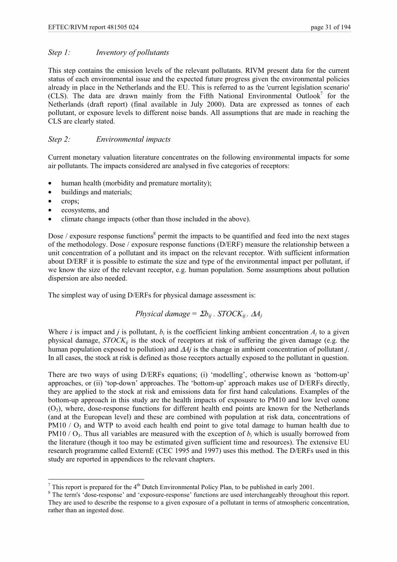
This step contains the emission levels of the relevant pollutants. RIVM present data for the currentstatus of each environmental issue and the expected future progress given the environmental policiesalready in place in the Netherlands and the EU. This is referred to as the 'current legislation scenario'(CLS). The data are drawn mainly from the Fifth National Environmental Outlook7 for theNetherlands (draft report) (final available in July 2000). Data are expressed as tonnes of eachpollutant, or exposure levels to different noise bands. All assumptions that are made in reaching theCLS are clearly stated.
Step 2: Environmental impacts
Current monetary valuation literature concentrates on the following environmental impacts for someair pollutants. The impacts considered are analysed in five categories of receptors:
• human health (morbidity and premature mortality);• buildings and materials;• crops;• ecosystems, and• climate change impacts (other than those included in the above).
Dose / exposure response functions8 permit the impacts to be quantified and feed into the next stagesof the methodology. Dose / exposure response functions (D/ERF) measure the relationship between aunit concentration of a pollutant and its impact on the relevant receptor. With sufficient informationabout D/ERF it is possible to estimate the size and type of the environmental impact per pollutant, ifwe know the size of the relevant receptor, e.g. human population. Some assumptions about pollutiondispersion are also needed.
The simplest way of using D/ERFs for physical damage assessment is:
Physical damage = Σbij . STOCKij.. ∆Aj
Where i is impact and j is pollutant, bi is the coefficient linking ambient concentration Aj to a givenphysical damage, STOCKij is the stock of receptors at risk of suffering the given damage (e.g. thehuman population exposed to pollution) and ∆Aj is the change in ambient concentration of pollutant j.In all cases, the stock at risk is defined as those receptors actually exposed to the pollutant in question.
There are two ways of using D/ERFs equations; (i) ‘modelling’, otherwise known as ‘bottom-up’approaches, or (ii) ‘top-down’ approaches. The ‘bottom-up’ approach makes use of D/ERFs directly,they are applied to the stock at risk and emissions data for first hand calculations. Examples of thebottom-up approach in this study are the health impacts of exposusre to PM10 and low level ozone(O3), where, dose-response functions for different health end points are known for the Netherlands(and at the European level) and these are combined with population at risk data, concentrations ofPM10 / O3 and WTP to avoid each health end point to give total damage to human health due toPM10 / O3. Thus all variables are measured with the exception of bi which is usually borrowed fromthe literature (though it too may be estimated given sufficient time and resources). The extensive EUresearch programme called ExternE (CEC 1995 and 1997) uses this method. The D/ERFs used in thisstudy are reported in appendices to the relevant chapters.
7 This report is prepared for the 4th Dutch Environmental Policy Plan, to be published in early 2001.8 The term's ‘dose-response’ and ‘exposure-response’ functions are used interchangeably throughout this report.They are used to describe the response to a given exposure of a pollutant in terms of atmospheric concentration,rather than an ingested dose.

page 32 of 194 EFTEC/RIVM report 481505 024
The ‘top-down’ approach makes a simplifying assumption that the relationship between emissionsand concentrations is linear and directly proportional. This implies that if emissions of a pollutantincrease by x%, the concentration of that pollutant in the area concerned is assumed to increase by x%as well, i.e.
∆Aj = ∆Ej
Where, ∆ is change in, Aj is ambient concentration and Ej is emissions of pollutant j. Combining thisassumption with that of a constant coefficient bi (implied in both approaches) implies that physicaldamages per unit of emissions are assumed constant in the ‘top-down’ approach. Therefore, it is notnecessary to use D/ERFs directly, but it suffices to use the average Euro per unit of pollutant, whichwas originally estimated using D/ERFs. Adopting the ‘top-down’ assumption of linearity is generallyjustifiable, as many validated models are linear, at least for primary pollutants. The ‘top-down’method bypasses Step 2 and uses the results of Step 3 directly. Thus we see that the ‘top-down’approach uses information and data from other studies that are brought together and applied tothe current context for secondary calculation. For purposes of transparency all D/ERFs embeddedwithin the unit damage values are reported at the end of the relevant sections (Section 4.4 onacidification) so that estimates may be compared and updated more easily as the literature develops.
Step 3: Monetary values
Following on from Step 2 there are also two ways of using monetary values to measure the damage ofpollutants. Since the ‘bottom-up’ approach measures the physical impact per unit of pollutant, thenecessary monetary value is that per physical impact (e.g. WTP to avoid a case of cardiovasculardisease). This is a first hand calculation of damage (e.g. Euro / impact). The difficulties with thisapproach lie in both finding the right estimates for WTP and in estimating the D/ERF. This is becausethe relationship between emissions and concentrations can vary across sites and over time, as do thereceptors or ‘stock’ exposed to the pollution. For examples of the ‘bottum-up’ approach see theanalysis on particulate matter and low level ozone.
The ‘top-down’ approach discussed in Step 2 conducts a secondary calculation for damage. The onlymonetary value the ‘top-down’ approach requires is the final damage value given in the form of Europer unit of pollutant. This is because physical and monetary measures of environmental impacts arealready embedded within the estimate of damage of Euro per unit of pollution, i.e. Euro / pollutantcomes from (Euro / impact) x (impact / pollutant). In order to make use of the ‘top-down’ approach, itis necessary to take ‘bottom-up’ step 3 results from other studies. This means the original values areapplied outside of the site context where the original study was carried out. Using the results of anoriginal study for another context / site, is called ‘benefits transfer’. For further details regardingbenefits transfer, refer to the Annex 2 on Benefits Transfer.
Due to the time and budget limitations of this study, it has been necessary to rely mainly on the ‘top-down’ approach to estimate the benefits of environmental control. For example, for air pollutants, wemake use of both ExternE (1995 and 1997) and AEA Technology (1999), studies which both followthe ‘bottom-up’ approach. For each environmental issue, we conduct a literature review of valuationstudies in the Netherlands and in the rest of Europe9 in order to pull out the most reliable 'willingnessto pay' (WTP) estimates to avoid environmental damage.
The majority of the studies to be used are conducted outside the Netherlands thus, the ‘willingness topay’ (WTP) estimates are adjusted to reflect Dutch WTP values. The rationale for the adjustments toWTP are given below together with an explanation of how it is achieved:
9 Techniques for the monetary valuation of environmental damage are not reviewed here. Detailed descriptionsof methodology can be found in Freeman (1993).

EFTEC/RIVM report 481505 024 page 33 of 194
• Spatial adjustment (e.g. adjusting UK WTP values to estimate Dutch WTP values): Ready et al(1999) suggest that where impacts are broadly distributed nationally, the nation-wide estimates ofpurchasing power parity (PPP) adjusted exchange rates provided by OECD are appropriate forthis task, and
• Intertemporal adjustment-past: (e.g. 1990 values to current 2000 values) by means of theharmonised consumer price index.
For further details of the WTP adjustments, refer to Annex 2 on Benefits Transfer.
Although benefits transfer is a practical method that significantly reduces the time and budgetrequirements for analysis, it should be remembered that the monetary values used in this way containuncertainties. The main uncertainty is that the validity of making the transfer is not known. Thisuncertainty differs from the confidence interval relevant to the estimate that is 'borrowed' for thetransfer.
It is a priority of this report to be very transparent with regard to the development of the unit damagevalues. Many assumptions are made and embedded in the damage per unit of emissions values, suchas dose / exposure response functions, as mentioned above. For the purposes of transparency, clearand concise statements of assumptions used are reported in the appendices at the end of the relevantsections.
Step 4: Monetary damage estimation and aggregation
Whether the ‘bottom-up’ or ‘top-down’ method is chosen, monetary damage estimation is a simpleprocedure and follows a typically multiplicative format. For the ‘bottom-up’ method, the relevantunits are the concentration of a pollutant (µg/m3, ppb, ppm). The units for the measurement of humanhealth impacts look like the following:
MonetaryDamage
= Σ(Pij . Bij . STOCKij . ∆Aij)
Euro = (Euro/impact) . (impact/person.µg/m3) . (persons) . (µg/m3)
Where Pi is the price of or willingness to pay to avoid the impact, and bij, STOCKij and ∆Aij are asgiven above.
Whilst for the 'top-down' approach, the aggregation would be as follows:
MonetaryDamage
= Σ(Pj . ∆Ej)
Euro = (Euro/tonne) (tonnes ofpollutant)
Where Ej denotes emissions of pollutant j and Pj is the unit damage value for pollutant j. Thus we seethat the unit damage values found in Step 3, are combined with the emissions data given in Step 1 togive the aggregate mean monetary value of the environmental impacts in the CLS. Aggregateddamage is estimated for 1995, 2010, 2020 and 2030.
The final product of the above process, i.e. Euro damage for each environmental issue can beinterpreted as the maximum Euro primary benefit from environmental control, i.e. the avoideddamage. Any secondary benefits of control should also be estimated and added to the avoided damageestimates. The total benefits of control can then be compared with the costs of control and contributeto decision making in environmental policy, when such information is available.
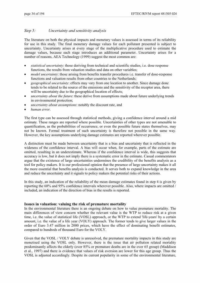
page 34 of 194 EFTEC/RIVM report 481505 024
Step 5: Uncertainty and sensitivity analysis
The literature on both the physical impacts and monetary values is assessed in terms of its reliabilityfor use in this study. The final monetary damage values for each pollutant presented is subject touncertainty. Uncertainty arises at every stage of the multiplicative procedure used to estimate thedamage values, because each stage introduces an additional parameter. Uncertainty arises for anumber of reasons, AEA Technology (1999) suggest the most common are:
• statistical uncertainty: those deriving from technical and scientific studies, i.e. dose responsefunctions, the results from valuation studies and data on other variables;
• model uncertainty: those arising from benefits transfer procedures i.e. transfer of dose-responsefunctions and valuation results from other countries to the Netherlands;
• geographical uncertainty: effects may vary from one location to another. Since damage donetends to be related to the source of the emissions and the sensitivity of the receptor area, therewill be uncertainty due to the geographical location of effects;
• uncertainty about the future: these derive from assumptions made about future underlying trendsin environmental protection;
• uncertainty about assumptions: notably the discount rate, and• human error.
The first type can be assessed through statistical methods, giving a confidence interval around a midestimate. These ranges are reported where possible. Uncertainties of other types are not amenable toquantification, as the probabilities of occurrence, or even the possible future states themselves, maynot be known. Formal treatment of such uncertainty is therefore not possible in the same way.However, the key assumptions underlying damage estimates are reported wherever possible.
A distinction must be made between uncertainty that is a bias and uncertainty that is reflected in thewideness of the confidence interval. A bias will occur when, for example, parts of the estimate areomitted, resulting in an underestimate. Whereas if the confidence interval is wide, this suggests thataccuracy is low, but it does not imply there is a systematic error in the estimate. Casual commentatorsargue that the existence of large uncertainties undermines the credibility of the benefits analysis as atool for policy makers. It is our professional opinion that the presence of large uncertainty makes it allthe more essential that benefits analysis is conducted. It serves both to expand knowledge in the areaand reduce the uncertainty and it signals to policy makers the potential risks of their actions.
In this study, an indication of the reliability of the mean damage estimates found in step 4 is given byreporting the 68% and 95% confidence intervals wherever possible. Also, where impacts are omitted /included, an indication of the direction of bias in the results is reported.
Issues in valuation: valuing the risk of premature mortalityIn the environmental literature there is an ongoing debate on how to value premature mortality. Themain differences of view concern whether the relevant value is the WTP to reduce risk at a giventime, i.e. the value of statistical life (VOSL) approach, or the WTP to extend 'life-years' by a certainamount, i.e. the value of a life year (VOLY) approach. The former tends to give larger values in theorder of Euro 3.47 million in 2000 prices, which have the effect of dominating benefit estimates,compared to hundreds of thousand Euro for the VOLY.
Given that the VOSL / VOLY debate is unresolved, the premature mortality impacts in this study aremonetised using the VOSL only. However, there is the issue that air pollution related mortalitypredominantly affects the elderly (over 85% or premature deaths are in the over 65 group) (Maddisonet al., 1997) and there is evidence that values of risk aversion are lower for this age group. Thus theVOSL is adjusted accordingly. Despite its current popularity in some of the environmental literature,

EFTEC/RIVM report 481505 024 page 35 of 194
the VOLY is not used. It is important to recognise that there are no VOLY estimates of any rigour forEurope. For a more detailed discussion of the issues surrounding the valuation of premature mortality,refer to Annex 3 on Valuing the Risk of Premature Mortality.
3.4 Public opinion methodologyThis section determines a ranking of environmental issues according to the surveys of Dutch publicattitudes towards the environment.
The rationale for turning to public opinion as an assessment procedure is twofold. Firstly, findingsfrom the various European and national surveys show that the environment remains a major concernfor the Dutch public. In 1986, 87% and in 1995, 80% see environmental protection as an 'urgent andimmediate problem’. Although in 1999 this level drops to 70%, these figures still demonstrate thatpublic opinion about the environment is consistently strong and not greatly influenced by media orpolitical attention.
Secondly, by using public opinion to rank the environmental issues, all Dutch citizens are weightedequally, they are effectively given an equal number of 'votes' on the environment. The final rankingachieved by this assessment is impartial to differences in variables that can affect economicassessments such as income.
Data are taken from the results of seven public opinion surveys, namely, SCP (1993, 1997), IISP(1993) and Eurobarometer (1992, 1995, 1996 and 1999).
The results of the surveys are compared to see if any trends can be identified in Dutch public opinionabout the environment.
The original surveys design the question in two main ways:
1) To obtain a percentage of respondents which agree or disagree to a particular statement, and
2) To find the national average of opinion when respondents are asked to rate a particular issue on asliding scale, for instance, 1-not worried to 4 – very worried.
For the first question type, percentages are taken only from those respondents who answer that theyfind an issue important, dangerous or serious. The percentages of people who gave these answers arethen summed, and a ranking order is presented. Where data are given as a national average, then theaverages are simply ranked in order of importance.
Although environmental issues used in the surveys correspond closely with the environmental issuesconsidered in this study, a few difficulties arise, particularly:
Incomplete ranking: Some issues are excluded from surveys, which means rankings are in effectincomplete, for example, land contamination. Exclusion from public opinion surveys does notnecessarily indicate they are given a low priority.
Broad categories: Most surveys cite air pollution as an environmental problem. However, reference isnot made to the specific pollutants causing the air pollution, such as particulate matter, low levelozone, etc. We assume that ‘air pollution’ represents both PM10 and low level ozone. We also assumethat ‘excessive use of pesticides, herbicides and fertilisers corresponds with eutrophication as definedin this study.
Over representation: Some environmental issues are expressed as a major concern at more than onelevel. For example, biodiversity loss is cited at the global, national and local level. In order to capturerepeated representation, the average of the percentage values given in the different levels is used.

page 36 of 194 EFTEC/RIVM report 481505 024
3.5 Disability adjusted life years’ (DALYs)The DALY methodology largely follows that of Murray and Lopez (1996). They develop the‘disability adjusted life years’ measure in order to assess the global disease burden and consequentlythe health policy priorities in different regions of the world. This health impact measure combinesyears of life lost and years lived with disease or disability that are weighted according to severity.
In the NEO5 framework adequate data and future projections are available for particulate matter, lowlevel ozone, noise, ultra-violet radiation, radon, home dampness and food borne infectious diseaseonly. For each relevant health outcome we calculate attributable risks by combining populationweighted exposure distributions with relative risk estimates derived from the epidemiologicalliterature. Subsequently for each health outcome the number of cases was estimated by combiningbaseline incidence rates with the attributive risks. Calculations of future disease burden are based onprojections of future population structure. We present the set of endpoints used to arrive at estimatesof attributable disease burden and the number of DALYs lost. Finally a total exposure attributabledisease burden was calculated by aggregating the number of DALYs for each health outcome. Thedisease burden associated with additional UV-exposure due to ozone layer degradation was calculatedby aggregating annual morbidity and mortality estimates of skin cancer and Dutch burden of diseasedata, (Melse et al., 2000). Statistical uncertainty was assessed using Monte Carlo techniques.
EFTEC/RIVM report 481505 024 page 37 of 194
4. Application of damage assessment methodology
The following sections devoted to the seven different environmental issues are organised in thefollowing order. For convenience the corresponding methodological step is indicated.
- brief overview of the environmental issue;
- identification of the sources of emissions and the most widely accepted impacts due to theemissions;
- definition of the scenarios used to represent the current and future status of the environmentalissue (Steps 1 and 2);
- summary of the literature review for WTP information, conducted to establish unit damagecosts for each pollutant (Step 3);
- estimation of the environmental damage due to each issue (Step 4);
- indication of the level of uncertainty attached to the results (Step 5), and
- appendix (where relevant) with the assumptions embedded in the analysis.

page 38 of 194 EFTEC/RIVM report 481505 024
4.1 Climate change4.1.1 The issueEmissions of greenhouse gases (GHG) are thought to lead to climate change. The main greenhousegases are, carbon dioxide (CO2), nitrous oxide (N2O) and methane (CH4). Three other gases are alsoconsidered to be GHGs, these are, hexafluorocarbons (HFC), perflurocarbons (PFC) andsulphurhexafluoride (SF6). Whilst still the subject of scientific uncertainty, the IntergovernmentalPanel on Climate Change (IPCC, 1995) suggests that a doubling of pre-industrial CO2 concentrationswould produce an aggregate economic loss of 1.5-2.0% of the world GNP. Although somecommentators argue that 'waiting' for better scientific evidence is justified, countries are currentlysigning up to climate change control strategies.
4.1.2 Source of emissionsCarbon dioxide is produced mainly as a result of the combustion of fossil fuels used for electricitygeneration and transport and in the industrial sector. The major sources of methane are agriculture,power generation, and from anaerobic digestion which takes place in landfill sites and bio-gasificationplants. It is worth noting that when methane is collected from waste disposal sites and burnt, it isconverted into carbon dioxide and water. Nitrous oxide is produced mainly as a result of industrialactivity and agriculture. Other radiatively active gases such as NOx, SO2, VOCs and CO are omittedfrom the review here.
4.1.3 Physical measure of impactsGreenhouse gases are not considered to cause significant direct damage to the environment or humanhealth. But, as concentrations increase and more heat is trapped in the atmosphere, global warming isexpected to occur and consequently affect the climate causing a number of potentially seriousimpacts, these are listed in Box 4.1.1.
Box 4.1.1 Possible climate change impacts- sea level rise;- change in agriculture, forests and fisheries;- change in energy, water, construction, transport and tourism sectors;- increased risk of disaster: changes in the frequency and severity of storms, floods,
droughts, hurricanes and precipitation levels;- change in biodiversity;- increased human morbidity and premature mortality, and- human migration.
Working group 2 of the IPCC is mainly responsible for assessing the impacts of global warming.Scientific research on global warming impacts has largely focused on the case of CO2 concentrationdoubling, i.e. the impacts of an atmospheric CO2 concentration of twice the pre-industrial level(2xCO2). Doubling is an arbitrary benchmark chosen solely for analytical convenience.
There is great uncertainty about the impacts of rising greenhouse gas concentrations on temperatureand climate. Issues of non-linearity, i.e. when changes in one variable cause more than proportionateimpact on another variable and irreversibility, i.e. changes that once set in motion cannot be reversed,add to the difficulty in measuring the global warming impacts. Also, some impacts may be moredependent on the rate of warming, rather than the absolute level of temperature. Other issues that alsoadd to the complexity of measurement are: regional variation i.e. some regions will suffer fromwarming whilst others will benefit at least for some sectors, and inertia in the climate system.
This last issue is due to the fact that atmospheric concentrations rather than emissions determine theamount of warming projected by the models. Thus long time lags and the difficulty of detecting

EFTEC/RIVM report 481505 024 page 39 of 194
climate change increase the difficulty of reliably determining the magnitude and timing of futureeffects before they begin to occur. Despite these shortcomings, the impacts of global warming areestimated. For a detailed analysis see Bruce et al., (1996).
Current legislation scenario: emissionsThe data for the greenhouse gases are taken from the NEO5 (draft report), the ‘medium growth’scenario (EC) is chosen, thus damage estimates (or maximum primary benefit estimates) areconservative. Results based on emissions data in the ‘high growth’ scenario are interpreted as the‘worst case scenario’ for the environment, damage estimates are reported in the sensitivity section.
The total emissions for all GHGs from the Netherlands are reported in Table 4.1.1. Table 4.1.1 alsogives the sectoral breakdown for CO2, CH4 and N2O.

page 40 of 194 EFTEC/RIVM report 481505 024
Table 4.1.1 Greenhouse gas emissions: current legislation scenarioCO2: (million tonnes)
1995 2010 2020 2030Total 180.2 198.3 213.1 233.3Energy 45.9 47.5 50.0 57.1Industry 44.3 45.2 49.3 53.7Transport 32.4 38.7 44.5 52.2Households 21.8 21.5 20.0 18.3Refineries 11.5 15.6 17.0 17.8Services 9.9 13.5 15.3 16.7Agriculture 9.4 10.4 11.0 11.6Other 2.5 3.0 3.0 3.0Waste management 1.5 2.0 2.0 2.0Construction 0.7 0.8 0.8 0.8Sewage treatment 0.1 0.1 0.1 0.1Water 0.0 0.0 0.0 0.0CH4: (thousand tonnes)Total 1172 703 537 462Waste management 479 217 102 51Agriculture 479 385 368 343Energy sector 178 73 38 38Households 18 16 16 16Industry 8 5 5 6Transport 6 3 2 2Other 5 5 5 5N2O: (thousand tonnes)Total 71.9 61.6 61.5 63.1Industry 31.7 32.9 34.2 35.8Agriculture 27.6 20.9 20.0 19.6Transport 7.1 2.6 2.2 2.6Other 5.0 5.0 5.0 5.0Energy sector 0.4 0.2 0.1 0.1Total per gas (million tonnes CO2-eq)CO2 180.2 198.3 213.1 233.3CH4 24.6 14.8 11.3 9.7N2O 22.3 19.1 19.1 19.6HFK 6.7 3 5.4 6.5PFC 2.1 0.9 1.1 1.2SF6 1.5 2.0 2.3 2.7Total 237.3 238.1 252.2 273.0Source: NEO5 (draft report), EC (medium growth).
4.1.4 Monetary measure of impactUnit damage values for carbonThere are a number of studies, which assess the monetised value of damage done from globalwarming, these are summarised in Table 4.1.2. As a consequence of the scientific focus, the studiestend to be based on the 2xCO2 scenario as well. The most studied aspects are the impacts onagriculture and the costs of sea level rise, with some studies on forestry. Several studies provide a firstorder assessment of the total global warming damage using a simple enumerative approach, i.e. thetotal damage is the sum of individual damage categories. This type of partial equilibrium approach
EFTEC/RIVM report 481505 024 page 41 of 194
means that the estimates do not include the feedback effects (e.g. the change in agricultural yields willinduce changes on the food, tobacco and textile industry). All of the economic assessmentsundertaken to date are incomplete as they exclude some impacts which are potentially important,including low-risk, high consequence events which are problematic to quantify and value. Despitesuch short-comings, professional judgement suggests that global warming impacts are recommendedfor monetary evaluation.
The relevant damage estimates are marginal damage, i.e. the damage done by increasing greenhousegas emissions now by a small amount. Computing marginal damage is not, however, straightforward(for an outline interpretation, refer to the Appendix at the end of this chapter, based on Fankhauser(1995)). The relevant concept is the present value of damage done from an increase in emissions,allowing for the fact that greenhouse gases are cumulative pollutants, i.e. an increase in emissionsnow resides in the atmosphere for a long period of time. Thus,
PV(D) = Σ∆Dt/∆E.(1+s)-t, t = 1...T
Where PV is present value, ∆ is change in, D is damage, E is emissions, s is the discount rate, t is time,and T is time horizon. The complexities involve:
• relating emissions to concentrations;• relating concentrations to radiative forcing and warming;• relating warming to damage (since the ratio of damages per tonne of gas is not the same as global
warming potentials - see the guide to climate change models at the end of this chapter), and• selecting the discount rate.
Two forms of estimate are produced in the literature: (i) estimates of actual damage arising at the pointin time when 2xCO2 occurs and arising from a small increase in emissions now, and (ii) a ‘shadow price’defined as the level of tax required to keep emissions on an optimal trajectory as estimated by themodeller. Because the estimates relate to damage or benefit at the time when 2xCO2 occurs, they are thendiscounted back to the present (see formula above) so that the choice of discount rate matters. Indeed, it isthe discount rate that largely accounts for the difference in estimates.
The results of a literature review of recent studies which assess the economic costs of global warming aresummarised in Table 4.1.2. Note that the estimates of marginal damage costs from global warming givenin Table 4.1.2 are for carbon only.
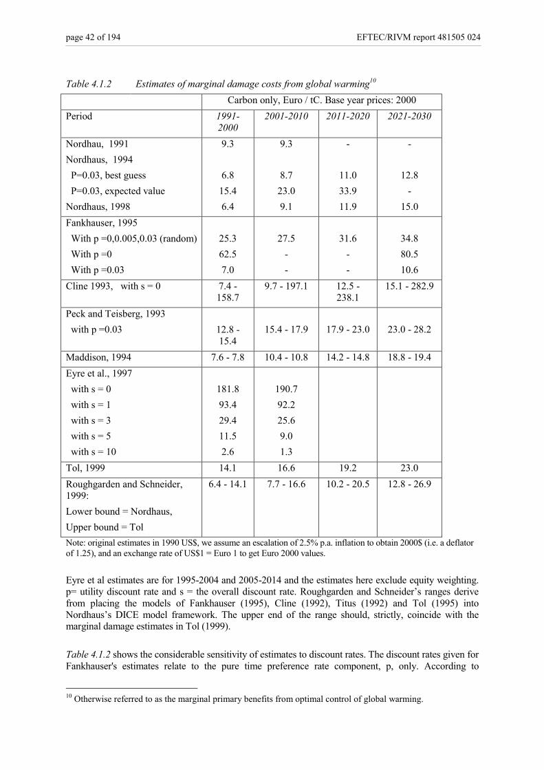
page 42 of 194 EFTEC/RIVM report 481505 024
Table 4.1.2 Estimates of marginal damage costs from global warming10
Carbon only, Euro / tC. Base year prices: 2000Period 1991-
20002001-2010 2011-2020 2021-2030
Nordhau, 1991Nordhaus, 1994 P=0.03, best guess P=0.03, expected valueNordhaus, 1998
9.3
6.815.46.4
9.3
8.723.09.1
-
11.033.911.9
-
12.8-
15.0Fankhauser, 1995 With p =0,0.005,0.03 (random) With p =0 With p =0.03
25.362.57.0
27.5--
31.6--
34.880.510.6
Cline 1993, with s = 0 7.4 -158.7
9.7 - 197.1 12.5 -238.1
15.1 - 282.9
Peck and Teisberg, 1993 with p =0.03 12.8 -
15.415.4 - 17.9 17.9 - 23.0 23.0 - 28.2
Maddison, 1994 7.6 - 7.8 10.4 - 10.8 14.2 - 14.8 18.8 - 19.4Eyre et al., 1997 with s = 0 with s = 1 with s = 3 with s = 5 with s = 10
181.893.429.411.52.6
190.792.225.69.01.3
Tol, 1999 14.1 16.6 19.2 23.0Roughgarden and Schneider,1999:Lower bound = Nordhaus,Upper bound = Tol
6.4 - 14.1 7.7 - 16.6 10.2 - 20.5 12.8 - 26.9
Note: original estimates in 1990 US$, we assume an escalation of 2.5% p.a. inflation to obtain 2000$ (i.e. a deflatorof 1.25), and an exchange rate of US$1 = Euro 1 to get Euro 2000 values.
Eyre et al estimates are for 1995-2004 and 2005-2014 and the estimates here exclude equity weighting.p= utility discount rate and s = the overall discount rate. Roughgarden and Schneider’s ranges derivefrom placing the models of Fankhauser (1995), Cline (1992), Titus (1992) and Tol (1995) intoNordhaus’s DICE model framework. The upper end of the range should, strictly, coincide with themarginal damage estimates in Tol (1999).
Table 4.1.2 shows the considerable sensitivity of estimates to discount rates. The discount rates given forFankhauser's estimates relate to the pure time preference rate component, p, only. According to
10 Otherwise referred to as the marginal primary benefits from optimal control of global warming.

EFTEC/RIVM report 481505 024 page 43 of 194
Fankhauser (1995) his social cost estimates based on the distribution of values for p are equivalent to a‘best guess’ value of 0.5% for p. To this must be added a value for the elasticity of the marginal utility ofincome multiplied by the expected growth rate. Fankhauser and Eyre et al take the elasticity to be aboutunity, so that the only variable is the expected long term economic growth rate of income per capita.Rabl (1996) suggests this is 1.6-1.8% pa, so that the discount rate would be 2.2 to 2.3%. Accordingly,the discount rate value in Eyre etc of 3% is more relevant for purposes of comparison.
Several factors explain the variability of the estimates in Table 4.1.2. First, the effect of differentdiscount rates is shown by the values of ‘p’, the utility discount rate. This rate discounts future utilityand it is usual to add this rate to the rate for discounting future income (consumption). Controversysurrounds the value of 'p' since some authors regard utility discounting as illicit, i.e. they set p=0. Theeffect is easily seen by comparing Fankhauser’s estimates with utility discount rates of zero and 3%:the difference is a factor of 9 in the damage estimate. The discount rate partly explains Cline’s largerange, but his estimates also reflect very high estimates of damage and a very long-term time horizon.The ‘central’ estimates are surprisingly similar. For 1991-2000 the damage estimate is around Euro7-15 tC but with the Eyre et al estimates being around twice this. Interestingly, the most recent studies,by Tol and Nordhaus suggest damage estimates lower than those previously estimated, althoughNordhaus’s estimate is fairly constant at Euro 6-9 (taking his preferred ‘best guess’). Tol’s 1999 paperis also probably the most careful recent estimate. Fankhauser's model has considerable attractionsbecause of its use of the discount rate as a random variable. This is shown here in the row withp=0, 0.005, 0.03, i.e. with a probability distribution assumed for ‘p’ taking values of 0%, 0.5% and3%.
Roughgarden and Schneider (1999) take four studies of total damages for 2xCO2 concentrations:Titus (1992), Cline (1992), Fankhauser (1995) and Tol (1995). Making slight modifications to thedamage estimates they then derive damage functions of the form:
Dt = a[∆Tt/w]2
Where Dt is the monetary value of damage done in year t expressed as a fraction of gross worldoutput, a is the fraction of world GNP lost for 2xCO2, ∆Tt is the change in earth surface temperature,w is the expected temperature change in oC for a 2xCO2 benchmark. Thus, in Tol’s case, for example,a = 0.02, i.e. 2xCO2 is expected to give rise to global output loss of 2%, and w is 2.5. These damagefunctions are put into Nordhaus’s DICE model to produce optimal carbon taxes, (i.e. marginal damageestimates) as shown in the final row of Table 4.1.2.
Recent work by Mendelsohn and Neumann (1999) suggests net benefits for impacts on the marketsector in the USA, and Mendelsohn (1996) has also suggested that this conclusion may hold true forthe world as a whole. This is not the position taken here. Also ignored is the effect of equity weightingon the estimates. For this debate see Fankhauser et al., (1997a, 1997b), Tol et al., (1996, 1999), Azar(1999), and Azar and Sterner (1996).
The authors acknowledge that the discount rates assumed in the economic studies of climate change willhave a significant impact on the results. Where marginal damage values are present values over theentire period, we assume discount rates of zero too low and 10 too high. Thus, marginal damages ofEuro 8 - 30 tC for the year 2000 and onwards seem defensible as a central range. The unit damagevalues assume damage to drylands, wetlands, ecosystems, agriculture, forestry, energy, water sector,amenity, human health and coastal regions.
The reliability of the recommended central marginal damage values is found using the confidence limitsaround these mean marginal damages. The upper value of the recommended central estimate, Euro30/tC, is very close to the estimates given by Fankhauser’s model (1995). Based on the 90% confidencelimit for his marginal damage values, we present a range of marginal damage values around the upper
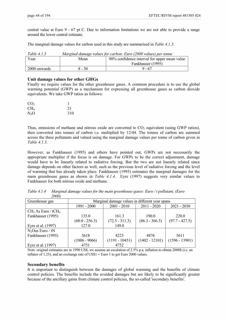
page 44 of 194 EFTEC/RIVM report 481505 024
central value at Euro 9 - 67 pt C. Due to information limitations we are not able to provide a rangearound the lower central estimate.
The marginal damage values for carbon used in this study are summarised in Table 4.1.3.
Table 4.1.3 Marginal damage values for carbon: Euro (2000 values) per tonneYear Mean 90% confidence interval for upper mean value
Fankhauser (1995)2000 onwards 8 - 30 9 - 67
Unit damage values for other GHGsFinally we require values for the other greenhouse gases. A common procedure is to use the globalwarming potential (GWP) as a mechanism for expressing all greenhouse gases as carbon dioxideequivalents. We take GWP ratios as follows:
CO2 1CH4 21N2O 310
Thus, emissions of methane and nitrous oxide are converted to CO2 equivalent (using GWP ratios),then converted into tonnes of carbon i.e. multiplied by 12/44. The tonnes of carbon are summedacross the three pollutants and valued using the marginal damage values per tonne of carbon given inTable 4.1.3.
However, as Fankhauser (1995) and others have pointed out, GWPs are not necessarily theappropriate multiplier if the focus is on damage. For GWPs to be the correct adjustment, damagewould have to be linearly related to radiative forcing. But the two are not linearly related sincedamage depends on other factors as well, such as the previous level of radiative forcing and the levelof warming that has already taken place. Fankhauser (1995) estimates the marginal damages for themain greenhouse gases as shown in Table 4.1.4. Eyre (1997) suggests very similar values toFankhauser for both nitrous oxide and methane.
Table 4.1.4 Marginal damage values for the main greenhouse gases: Euro / t pollutant, (Euro2000)
Greenhouse gas Marginal damage values in different year spans1991 - 2000 2001 - 2010 2011 - 2020 2021 - 2030
CH4 As Euro / tCH4Fankhauser (1995)
Eyre et al. (1997)
135.0(60.0 - 256.3)
127.0
161.3(72.5 - 311.3)
149.8
190.0(86.3 - 366.3)
220.0(97.7 - 427.5)
N2Oas Euro / tNFankhauser (1995)
Eyre et al. (1997)
3618(1006 - 9066)
4751
4223(1191 - 10451)
4752
4876(1402 - 12101)
5611(1596 - 13901)
Note: original estimates are in 1990 US$, we assume an escalation of 2.5% p.a. inflation to obtain 2000$ (i.e. aninflator of 1.25), and an exchange rate of US$1 = Euro 1 to get Euro 2000 values.
Secondary benefitsIt is important to distinguish between the damages of global warming and the benefits of climatecontrol policies. The benefits include the avoided damages but are likely to be significantly greaterbecause of the ancillary gains from climate control policies, the so-called 'secondary benefits'.

EFTEC/RIVM report 481505 024 page 45 of 194
Secondary benefits arise because the control of carbon dioxide is likely to involve policies, which willalso reduce other pollutants. Most of the literature has concentrated on the effect of climate controlpolicies on jointly produced pollutants such as NOx, SOx etc. However, it can be argued that climatechange policies may also secure gains in employment and in other social effects such as reduced noisenuisance and accidents. How far gains in employment should be credited to climate policies, however,is open to debate. If such gains could be secured anyway, i.e. independently of climate change policy,then it would not appear to be reasonable to add them in as benefits of a climate policy. If they canonly be secured by a climate policy, then their addition seems appropriate. Thus the total benefits i.e.primary and secondary benefits of a policy measure to control greenhouse gases are likely to exceedthe avoided damage i.e. primary benefits of control.
Table 4.1.5 reveals a wide disparity of estimates. US estimates are, with some exceptions, notablysmaller than European estimates. Part of the problem arises from slightly different methodologies: theEuropean studies tend to be ‘snapshot’ pictures of the amount (and value) of secondary pollutantsemitted at any one time. These are then expressed per tonne of carbon. However, for policy purposes itis preferable to estimate such benefits as being incremental to any policies currently ‘in the pipeline’ forsecondary pollution policy. Since most secondary pollutants are the subject of independent policies,emissions can be expected to fall over time, so that climate change policies will secure a further butsmaller incremental fall in the future.
The evaluation of the climate change issue presented in this report relates to current damage in 1995 andfuture damage in 2010, 2020 and 2030. This type of analysis makes use of the marginal damage valuesreported earlier, it does not require the inclusion of the secondary benefit estimates reported in Table4.1.5. However, when evaluation of global warming control policies is conducted, it is important toconsider the secondary benefits of those policies.
Table 4.1.5 Secondary (emission) benefits per tC as a multiple of primary benefitsStudy Country Ancillary
benefitsEuro / tC
Ancillary benefitsas a multiple ofprimary benefits (at Euro 30 / tC)
Comment
Ayres and Walter,1991
USA 165 5.5
Boyd et al., 1995 USA 40 1.3 Criteria pollutantsBurtraw and Toman,1998
USA <10 <0.33 Judgmental assessmentof prior studies
Burtraw et al.,1999 USA 3 0.1 SO2, NOx onlyDowlatabadi etal.,1993
USA 3 0.1 SO2, NOx, PM
Goulder, 1993;Scheraga and Leary,1993
USA 33 1.1 SO2, NOx, PM, Pb,CO, VOCs
Lutter and Shogren,1999
USA 300 10.0 See text
Rowe et al., 1995 USA 24 0.8 SO2, NOx, PMViscusi et al., 1994 USA 88 2.9 Criteria pollutantsBarker, 1993 UK 44 - 201 1.5-6.7 Relies on Pearce 1992Pearce, 1992 UK 195 6.5 SO2, NOx, PMAyres and Walter,1991
Germany
312 10.4
Alfsen, 1992 Norway 102 - 146 3.4-4.9RIVM et al., 2000 EU 53 - 79 1.8-2.6 General equilibrium
modelSources: OECD (1999); Lutter and Shogren (1999); RIVM et al., (2000).

page 46 of 194 EFTEC/RIVM report 481505 024
4.1.5 Aggregate monetary damage estimateDue to the existence of an international climate change treaty the relevant estimate is damage to theworld caused by greenhouse gas emissions from the Netherlands.
The following tables present the results of applying the shadow values in Table 4.1.3 to the currentlegislation scenario (CLS) emissions for the greenhouse gases given in Table 4.1.1. The method usedconverts all greenhouse gases into carbon equivalents, using the global warming potentials. Table4.1.6 reports the mean damage to the world due to Dutch GHG emissions in the years 1995, 2010,2020 and 2030. All values are given in millions of Euro (2000 prices).
Table 4.1.6 Mean damage to world due to Dutch GHG emissions: Euro million1995 2010 2020 2030
CO2 as C 393 - 1474 433 - 1622 465 - 1743 509 – 1908CH4 as Ceq 54 - 201 32 - 121 25 - 92 21 – 79N2O as Ceq 49 - 182 42 - 156 42 - 156 43 – 160Subtotal 495 - 1858 507 - 1900 531 - 1991 573 – 2148HFC as Ceq 15 - 55 7 - 26 12 - 44 14 – 53PFC as Ceq 5 - 17 2 - 7 2 - 9 3 – 10SF6 as Ceq 3 - 12 4 - 16 5 - 19 6 – 22Total 518 - 1942 519 - 1948 550 - 2064 596 – 2234Note: the range of damage estimates presented in Table 4.1.6 are based on the low - upper central marginaldamage values, i.e. Euro 8 - 30 /tC.
Table 4.1.7 presents the mean damage to the world due to the emissions of CO2, CH4 and N2O fromthe Netherlands by sector, in the years, 1995, 2000, 2010 and 2020. Sectoral emission data for theother GHGs are not available. The greatest level of damage is caused by carbon dioxide emissionsfrom the power generation, industrial and transport sectors. One of the most striking changes indamage between the years 1995 and 2020 is the level of damage caused by methane emissions fromthe waste sector which goes down significantly.

EFTEC/RIVM report 481505 024 page 47 of 194
Table 4.1.7 Sectoral mean damage due to CO2, CH4 and N2O. Euro million (2000 prices)CO2 as C
1995 2010 2020 2030Waste management 12.6 16.1 16.1 16.1Construction 5.8 6.6 6.6 6.4Households 178.6 176.1 163.9 149.6Water 0.2 0.0 0.0 0.0Energy 375.4 388.6 409.1 466.8Services 81.4 110.5 124.8 136.8Industry 362.2 369.5 403.4 439.3Agriculture 76.8 84.9 90.0 95.3Other 20.4 24.5 24.5 24.5Refineries 94.1 127.9 139.2 145.7Sewage treatment 1.0 1.2 1.2 1.2Transport 265.4 316.5 364.4 427.2Total 1474.0 1622.4 1743.3 1908.8CH4 as CeqWaste management 82.3 37.3 17.6 8.8Households 3.0 2.8 2.8 2.8Energy sector 30.6 12.5 6.5 6.5Industry 1.3 0.8 0.9 1.0Agriculture 82.2 66.2 63.3 59.0Other 0.9 0.8 0.8 0.8Transport 1.0 0.5 0.4 0.4Total 201.3 120.9 92.2 79.3N2O as CeqEnergy sector 1.0 0.5 0.3 0.3Industry 80.4 83.3 86.6 90.7Agriculture 70.0 53.0 50.8 49.7Other 12.8 12.6 12.6 12.6Transport 18.1 6.7 5.6 6.7Total 182.3 156.2 155.9 160.1Note: for clarity damage estimates presented in Table 4.1.7 are based on the upper central unit damage value fora tonne of C only, i.e. Euro 30/tC.
Finally, Table 4.1.8 gives the mean damage to the world due to Dutch emissions of the maingreenhouse gases by sector. The results show that between the years 1995 to 2020, the sectors thatcontribute most to the climate change problem from the Netherlands are, in descending order:industry, power generation and transport followed by agriculture. The order is held throughout theentire period. Although, the percentage share of environmental damage due to the industrial sectordoes increase slightly from 23.8% to 24.8%, whilst the power generation sector maintains a constantshare of 22.0%. The transport sector increases from 15.3% to 20.2% and the agriculture sectormaintains a constant share of 12%.
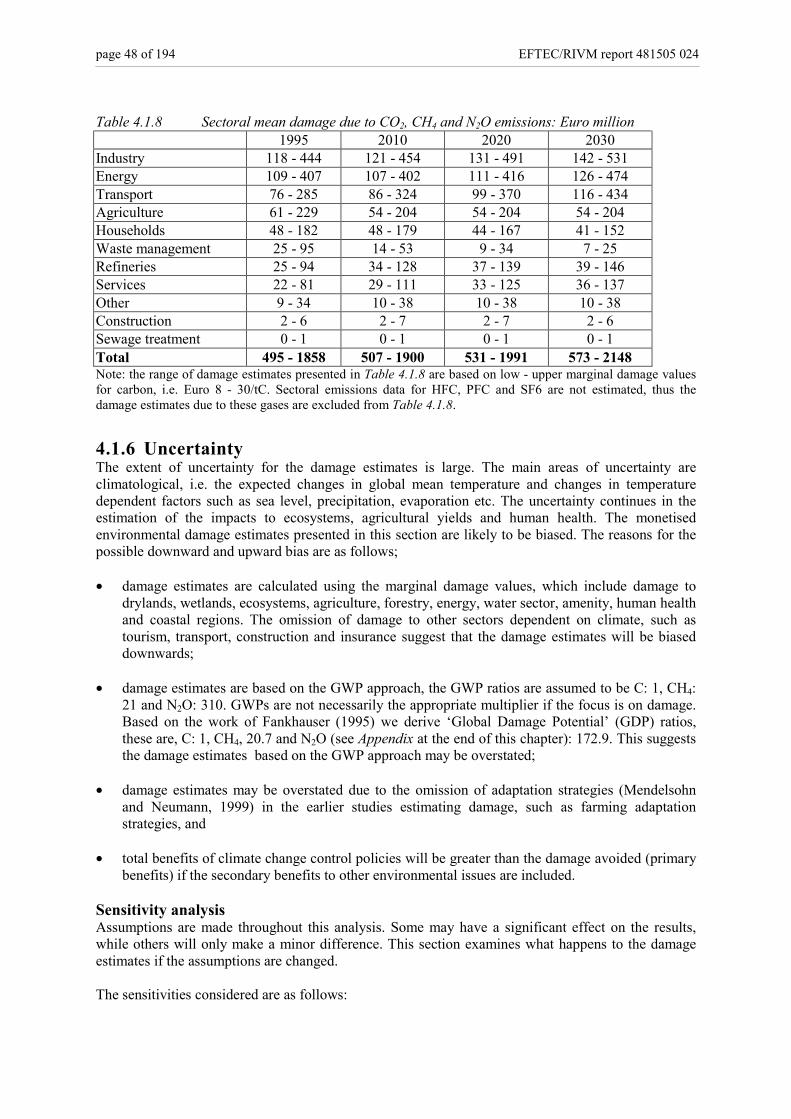
page 48 of 194 EFTEC/RIVM report 481505 024
Table 4.1.8 Sectoral mean damage due to CO2, CH4 and N2O emissions: Euro million1995 2010 2020 2030
Industry 118 - 444 121 - 454 131 - 491 142 - 531Energy 109 - 407 107 - 402 111 - 416 126 - 474Transport 76 - 285 86 - 324 99 - 370 116 - 434Agriculture 61 - 229 54 - 204 54 - 204 54 - 204Households 48 - 182 48 - 179 44 - 167 41 - 152Waste management 25 - 95 14 - 53 9 - 34 7 - 25Refineries 25 - 94 34 - 128 37 - 139 39 - 146Services 22 - 81 29 - 111 33 - 125 36 - 137Other 9 - 34 10 - 38 10 - 38 10 - 38Construction 2 - 6 2 - 7 2 - 7 2 - 6Sewage treatment 0 - 1 0 - 1 0 - 1 0 - 1Total 495 - 1858 507 - 1900 531 - 1991 573 - 2148Note: the range of damage estimates presented in Table 4.1.8 are based on low - upper marginal damage valuesfor carbon, i.e. Euro 8 - 30/tC. Sectoral emissions data for HFC, PFC and SF6 are not estimated, thus thedamage estimates due to these gases are excluded from Table 4.1.8.
4.1.6 UncertaintyThe extent of uncertainty for the damage estimates is large. The main areas of uncertainty areclimatological, i.e. the expected changes in global mean temperature and changes in temperaturedependent factors such as sea level, precipitation, evaporation etc. The uncertainty continues in theestimation of the impacts to ecosystems, agricultural yields and human health. The monetisedenvironmental damage estimates presented in this section are likely to be biased. The reasons for thepossible downward and upward bias are as follows;
• damage estimates are calculated using the marginal damage values, which include damage todrylands, wetlands, ecosystems, agriculture, forestry, energy, water sector, amenity, human healthand coastal regions. The omission of damage to other sectors dependent on climate, such astourism, transport, construction and insurance suggest that the damage estimates will be biaseddownwards;
• damage estimates are based on the GWP approach, the GWP ratios are assumed to be C: 1, CH4:21 and N2O: 310. GWPs are not necessarily the appropriate multiplier if the focus is on damage.Based on the work of Fankhauser (1995) we derive ‘Global Damage Potential’ (GDP) ratios,these are, C: 1, CH4, 20.7 and N2O (see Appendix at the end of this chapter): 172.9. This suggeststhe damage estimates based on the GWP approach may be overstated;
• damage estimates may be overstated due to the omission of adaptation strategies (Mendelsohnand Neumann, 1999) in the earlier studies estimating damage, such as farming adaptationstrategies, and
• total benefits of climate change control policies will be greater than the damage avoided (primarybenefits) if the secondary benefits to other environmental issues are included.
Sensitivity analysisAssumptions are made throughout this analysis. Some may have a significant effect on the results,while others will only make a minor difference. This section examines what happens to the damageestimates if the assumptions are changed.
The sensitivities considered are as follows:

EFTEC/RIVM report 481505 024 page 49 of 194
• effect of using the high growth scenario for greenhouse gas emissions,• effect of using the GDP approach to damage assessment, and• assume high discount rate, s=10%.
We also present estimates based on lower and upper marginal damage values. The results of thesensitivities are presented in Table 4.1.9.
Table 4.1.9 Sensitivity test 1: Mean, lower, upper damage caused by GHGs: Euromillion
1995 2010 2020 2030Current legislation scenario estimateGWP approach: mean marginal unitdamage value: Euro 30/tC
1942 1948 2064 2234
Sensitivities
(i) lower and upper values around themean, Euro 30/tC, Euro 9 - 67/tCrespectively;(ii) high growth scenario;(iii) GDP approach: mean marginal unitdamage values per tC, per tCH4 and pertN;(iv) GDP approach: lower and uppervalues;(v) high discount rate, s= 10%, i.e.marginal damage values becomes Euro1.9 / tC
583 - 4337
19421488
474 - 3284124
584 -4350
20341738
575 -4000126
619 -4609
22192035
677 -4675132
670 -4988
25022425
809 -5582141
From the sensitivity analysis, we can conclude the following:
• the mean marginal damage value used in this study, (Euro 30 /tC) is supported by the work ofFankhauser (1995). The reliability of these values is measured by presenting damage estimatesbased on the lower and upper 90% confidence limit. Table 4.1.9 shows that the damage estimatesfor climate change can be estimated to within a factor of roughly 2 (90% confidence interval).Thus, the damage estimates presented should be interpreted as a rough assessment of the order ofmagnitude only.
• estimates based on the high growth scenario for greenhouse gas emissions (Fifth NationalEnvironmental Outlook, draft) may be interpreted as a 'worst case scenario for the environment.The damage estimates are greater than for the medium growth scenario by 4% in 2010, 7% in2020 and 11% in 2030.
• in the main analysis we assume all greenhouse gases are converted to carbon equivalents, byusing their respective GWP ratios. Here we compare these results with the results derived fromvaluing the individual GHGs with their respective marginal damage value, i.e. Euro / tC, Euro /tCH4, and Euro / tN. Note carbon dioxide is converted into tonnes of carbon, and nitrous oxide isconverted into tonnes of nitrogen, by using their respective, relative molecular weights. Changingthe approach to valuing GHGs, i.e. the GWP approach: Euro / tC for all GHGs, or using the GDPapproach: Euro / t pollutants for the different GHGs, makes very little difference to the outcome.For example, comparing the mean results in 1995, the GWP approach, suggests environmentaldamage is some Euro 1.9 billion, whilst using the GDP approach the results are given as Euro 1.5billion. However, over time the damage estimates based on the GDP approach become greater

page 50 of 194 EFTEC/RIVM report 481505 024
than the damage estimates based on the GWP approach. This is explained by the rising marginaldamage values per pollutant over time, see Table 4.1.10, compared to the constant marginaldamage values assumed in the GWP approach, i.e. Euro 30/tC. Estimates based on the GDPapproach are an underestimate because they assume damage caused by emissions of CO2, CH4and N2O only.
Table 4.1.10 Adjusted marginal damage values used in the GDP approach: Euro 20001991 - 2000 2001 - 10 2011 - 20 2021 - 30
C: mean Euro / tC 25.4 28.5 31.6 34.8CH4: mean Euro / tCH4 135.0 161.3 190.0 220.0N: mean Euro / tN 3618.8 4223.8 4876.3 5611.3Note: original values adjusted by 2.5% p.a. i.e. the inflator 1.25, Financial exchange rate in Jan 2000: US$ =Euro 1.
• the final sensitivity test challenges the discount rate assumption. Assumptions about discountrates will have a major impact on the final results. There is no consensus on which discount rateto use. (Thus it is possible to choose either to not monetise damages or monetise climate changedamages using a large range of values). It is our professional opinion that discount rates of zeroare unrealistic and 10% is high. In the main analysis we assume a discount rate between 0-10. Inthe sensitivity we present results based the discount rate 10%.

EFTEC/RIVM report 481505 024 page 51 of 194
Appendix Guide to economic models of climate change damage
Economic damage estimates: underlying modelsAssumption: The rise in sea levels connected with a warmer climate will threaten low lying coastalregions. Sea level rise will particularly affect densely populated coastlines, and small island states.Most studies agree, in principle, that damage estimates should be based on the assumption of a costefficient response. That is, damage should be kept at a minimum through appropriate adaptationmeasures. This might include the erection of sea defences, the development of heat resistant crops,changes in agricultural practice and forest management, the construction of water storage andirrigation systems, the adaptation of houses, etc (Fankhauser, 1995). Unfortunately, while undisputedas a general idea, data limitations do not always permit the implementation of optimal adaptationstrategies when it comes to actual damage calculations. Thus it is assumed, for simplicity that noadjustments are taken at all, or that current service levels are maintained.
The underlying models for the economic damage estimates are fairly complex. The following is anoutline interpretation.
The models deal with small ('marginal') increases in emissions in a base period (e.g. now). This leads toan increase in atmospheric concentrations
∂Ci(s)/∂E(0)
where s is the time of the concentration, 0 is the base year of emission.
In turn, changed concentrations give rise to changed temperatures which depend on the radiative forcingof the gas, concentrations of other gases, climatic feedbacks and the inertia of the climate system:
∂T(t)/∂Ci(s), for t>s.
Increased temperatures give rise to (marginal) damage
∂D(t)/∂T(t).
Taking all the links together, the incremental damage done by a marginal emission at time t now will be:
∂D(t)/∂Ei(0) = ∂D(t)/∂T(t).�0,t {∂T(t)/∂Ci(s).∂Ci(s)/∂E(0)} ds
The marginal damage costs of an incremental tonne of emissions are
Ki = �0,τ[∂D(t)/∂Ei(0)].e-rt.dt
since damage done is cumulative (i.e. occurs as long as the gas remains in the atmosphere) and needs tobe discounted back to the present. r is the discount rate.
So,
Ki = �0,τ[∂D(t)/∂T(t).�0,t {∂T(t)/∂Ci(s).∂Ci(s)/∂E(0)} ds]e-rt.dt

page 52 of 194 EFTEC/RIVM report 481505 024
Damage and Radiative ForcingThe ratio of marginal damage from gas i, relative to CO2, will be the same as the ratio of GWPs if andonly if damage is a linear function of radiative forcing. But this is not true, since the damage from a givenincrease in radiative forcing will depend on previous levels of forcing and the degree of warming alreadyencountered.
As an example, Fankhauser (1995) has an annual damage function taking the form:
Dt = kt {Tt/Λ)γ.(1+ø)t*-t
where T in this case is surface temperature, Λ is the amount of warming associated with a doubling ofCO2 (in Fankhauser's case, 2.5o), t* is the time this is expected to occur (2050), kt is the economic damagedone by 2xCO2. Parameter γ is the relationship between temperature and damage, i.e. if temperature risesby 1%, damage rises by γ%. ø is a factor which makes impacts greater if they occur before t* and lower ifthey occur after t* - a rough attempt to account for damage being related to speed of change.
Thus, if 2xCO2 damage occurs in 2050 then damage = kt since t*=t and Tt = 2.5oC. Fankhauser (1995)adopts the following values based on the scientific and economic literature:
Λ = 2.5o
t* = 2050γ = range 1 to 3, with best guess 1.3ø is random with best guess of 0.006Kt is ‘bottom up’ procedure of aggregating individual damages. Damages are adjusted for population andeconomic growth.
In any period t, then, annual damage is given by
Dt = $270.109.(Tt/2.5)1.3
The model is not linear. Atmospheric concentrations are linear with respect to emissions; forcing islogarithmic in CO2 and has a quadratic form for CH4 and N20 (following IPCC); temperature change islinear with forcing; and damages are not linear with temperature. Thus use of forcing ratios to measurethe relative contributions of different gases to damage is misleading. An illustration is taken fromFankhauser (1995). The latest GWPs and global damage potentials are reported in Table 4.1.11.
Table 4.1.11 Global warming potential and global damage potential ratiosGas Global warming potential
ratios (100 years)Global damage potential ratios
Fankhauser (1995)CO2 1 1CH4 21 20.7N2O 310 172.9Note; to estimate global damage potentials, i) take marginal damage values for C, CH4 and N given in Table 4.1.3and Table 4.1.5, for the years 2001 - 2010; i.e. Euro 28.5/tC, Euro 161.3/ tCH4 and Euro 4223.8/tN; ii) convert tomarginal damage values for a tonne of CO2, CH4 and N2O, i.e. Euro 7.8/tCO2, Euro 161.3/tCH4 and Euro1343.9/tN2O; iii) estimate global damage potential ratios, i.e. divide marginal damage values for CO2 into values forCH4 and N2O.
EFTEC/RIVM report 481505 024 page 53 of 194
4.2 Acidification4.2.1 The issueThe primary pollutants, sulphur dioxide (SO2), nitrogen oxides (NOx) and ammonia (NH3) togetherwith their reaction products lead, after their deposition, to changes in the chemical composition of the‘acidification’. Their concentration in the air can cause impacts to human health.
4.2.2 Source of emissionsThe largest source of anthropogenic nitrogen oxides is the transport sector. This accounts for 63% ofall NOx emissions in the Netherlands. Other important sources are industry (12%) and the energysector (12%). Sulphur dioxide is produced mainly as a result of industrial activity, i.e. a by-product ofpower generation (12%), refineries (43%) and manufacturing (21%). The contribution of transport isagain significant (20%). By far the largest source of atmospheric ammonia is agricultural activity(94%) with consumers, industry and power generation contributing very small amounts.
4.2.3 Physical measure of impactsThere are five major receptors of air pollution: human health, crops, materials damage, ecosystemdamage and visibility impairment. However only the initial three can be quantified with any certaintyat this stage. Thus overall damages across the three receptors are estimated and given as the likelybenefits of the reduction in emissions. Table 4.2.1 outlines the main receptors of damage fromacidifying emissions, providing a brief description of each impact and the pollutant responsible. Table4.2.1 also describes those impacts omitted from economic valuation, due to either the currentscientific or economic uncertainty.
Note that the effects of ammonia are covered under other pollutants i.e. aerosols, N deposition, acidicdeposition. Impacts included are health (morbidity and premature mortality), fertilisation impact onagriculture. Impacts to ecosystems are excluded. However for eutrophication impacts, refer toChapter 4.6.
Recommended D/ERFs are given in full in the Appendix to this chapter. If it is assumed to be a linearrelationship, then for simplicity, only the D/ERF coefficient b, is reported. Unless describedotherwise, b, should be interpreted as the increase in annual incidence of each impact. For example,for morbidity, b is the number of cases per µg/m3 per year over a given population and for mortality, bis the % change in mortality rate per µg/m3 per year.

page 54 of 194 EFTEC/RIVM report 481505 024
Table 4.2.1 Environmental impacts of SOx, NOx and NH3
Impact receptor SOx NOx
Impacts quantifiedHuman health Direct damage
Indirect damage through sulphates(SO4 and SO2 aerosols)
Evidence of direct damage ismixedIndirect damage throughnitrates (NO3 aerosols) andozone, (O3)
Crops Fertilisation effect at lowconcentrationsDamage at high concentrations
Fertilisation effect (Ndeposition from NOx andNH3)
Materials Damage (SO2) No effect
Impacts not quantifiedEcosystem Damage Not known
Visibility Possible reduced visibility due toincreased air pollution
Possible reduced visibility dueto increased air pollution
Materials Effects on cultural assets (SO2)Damage to steel in reinforcedconcrete (SO2)
No effect
Agriculture Indirect effects on livestock (SO2) No effect
Human health No effect Indirect damage throughozone, (O3): see low levelozone for analysis.
Forests No effect Maybe some beneficial effect
Crops All pollutants: Interactions between pollutants, with pests, pathogensand climate (i.e. the negative impact of SO2 on global warming isomitted
Ecosystems Excess N deposition (from NOx and NH3 emissions) may harmecosystems through the effects of eutrophication.
The analysis here follows the ‘top-down’ approach described in the methodology (see Section 3.3).This means that D/ERFs are not used directly but are embedded within the unit damage values for theacidifying pollutants. For details of the D/ERFs used to establish unit damage values (and otherassumptions, such as the ‘stock at risk’), refer to the Appendix at the end of this chapter.
Current legislation scenario: emissionsThe data for the acidifying pollutants are drawn from the NEO5 (draft report), using the mediumscenario (‘EC’). Total emissions for SO2, NOx and NH3 from the Netherlands are reported in Table4.2.2. Table 4.2.2 also gives the sectoral breakdown of emissions sources.

EFTEC/RIVM report 481505 024 page 55 of 194
Table 4.2.2 Gases contributing to acidification: current legislation scenarioYear 1995 2010 2020 2030SO2: 1000 tonnesWaste 0.5 0.3 0.3 0.3Energy 16.7 9.8 8.6 10.5Industry 29.8 23.8 24.7 25.7Other 5.7 2.7 2.8 2.8Refineries 61.2 21.0 22.0 22.3Transport 29.9 13.7 15.4 17.2Total 143.8 71.2 73.8 78.6NOx: 1000 tonnesHouseholds 22.3 14.4 12.0 9.8Energy 58.1 23.8 25.4 25.4Services 8.1 7.6 7.4 7.0Industry 61.2 42.5 42.2 42.2Agriculture 10.3 12.0 9.5 7.5Other 3.8 2.4 2.6 2.6Refineries 17.7 8.1 8.2 8.2Transport 313.1 161.2 149.3 173.5Total 494.6 272.1 256.6 276.2NH3: 1000 tonnesHouseholds 6.7 7.4 7.8 8.2Industry 4.1 4.1 4.3 4.7Agriculture 176.9 143.0 133.4 128.0Other 0.6 0.7 0.8 0.8Total 188.4 155.2 146.3 141.7Source: NEO5 (draft report).
4.2.4 Monetary measure of impactDue to the existence of an international treaty for transboundary air pollution, the relevant estimate is thedamage to the ‘world’ due to emissions from the Netherlands.
It is also of interest to estimate the damage to the Netherlands from acidifiying pollutants released fromthe Netherlands and other countries and deposited in the Netherlands. In order to achieve this it isnecessary to know the relationship between domestic emissions and deposition in the Netherlands, aswell as foreign emissions and deposition in the Netherlands. Through impact measurement and valuation,it is then possible to estimate a damage per tonne deposited in the Netherlands. In order to achieve this,data have been combined from a variety of sources. Emissions data for the Netherlands for each of theacidifying pollutants have been provided by RIVM (Table 4.2.2 above). This has been used inconjunction with the EMEP transfer matrices, MSC-W (1995), which allow us to estimate the proportionof emissions from the Netherlands which are deposited within and outside the country and thereforedamage caused by the Netherlands within and outside the country. The relevant extracts from the EMEPdata are provided in Table 4.2.3 below.

page 56 of 194 EFTEC/RIVM report 481505 024
Table 4.2.3 Geographic depositions of pollutants emitted from the Netherlands (1996) (as a percentage of emissions from the Netherlands)
Pollutant Receiving countryNetherlands Elsewhere
NOx (as N) 5% 95%SO2 (as S) 14% 86%NH3 (as N) 43% 57%Source: http://projects.dnmi.no/-emep/
The reverse can also be estimated, i.e. the depositions to the Netherlands, caused by the Netherlands andby other countries. The data are provided in Table 4.2.4 below.
Table 4.2.4 Sources of emissions of acidifying depositions to the Netherlands (1996) (as a percentage of all depositions in the Netherlands)
Pollutant Source of emissionsNetherlands Elsewhere
NOx (as N) 17% 83%SO2 (as S) 15% 85%NH3 (as N) 75% 25%Source: http://projects.dnmi.no/-emep/
Unit damage values for SO2 and NOx and NH3Unit damage values for the acidifying pollutants have been based on the most recent ExternE report(1997) for the Netherlands, with some adjustments. The ExternE report estimates damages frompollutants emitted from the Netherlands for different fuel cycles. This produces a range of unitdamage estimates, depending on the location of emissions and therefore depositions. We have usedthe results of the ExternE dispersion modelling exercise, but have made the following adjustments tothe value estimates:
1. Notably, our estimates for mortality effects are based on acute mortality only. Chronic mortalityeffects are excluded due to the high scientific uncertainty surrounding these estimates, which arebased on a single study (Pope et al, 1995) and have been interpreted in several different ways.Moreover, it is not clear how a reduction in life expectancy should be valued. The ‘value ofstatistical life’ (VOSL) approach is based on valuations of mortality risk reduction, as is the ‘value oflife year’ (VOLY) approach which is derived from this. There is, in fact, only a single study whichattempts to value changes in life expectancy (Johannesson and Johansson, 1996). The resultingestimate of willingness to pay for an increase in life expectancy of one year is approximately $600-1,500. However, extrapolating results from a single study in a single country (Sweden) is highlyuncertain. Further original valuation research will undoubtedly be needed as the scientific estimatesof chronic mortality effects improve. In our professional opinion, the current scientific andeconomic research in this area is too uncertain to be recommended for valuation at this time. Theseeffects are therefore excluded from the current analysis.
2. Valuation of acute mortality effects for the over 65 age group is based on an age-adjusted VOSL (seeAnnex 3 on Valuing Risk of Premature Mortality for further details).
3. The unit values for a range of morbidity impacts have been taken from CSERGE et al (1999). Theseare more up-to-date estimates, and are based on a valuation study of the Netherlands specifically,whereas the values used in ExternE are adjusted cost of illness values taken from the USA. TheCSERGE et al values are therefore likely to be much more accurate. These values are summarised inAnnex 4 on Monetary Valuation of Health Effects.

EFTEC/RIVM report 481505 024 page 57 of 194
The unit values resulting from these adjustments are summarised in Table 4.2.5 below.
Table 4.2.5 Unit values for acidifying pollutants (Euro/tonne)Pollutant Effect Unit Value
(Euro/tonne)Lower upper
NOx Mortality (via nitrates) 1,374 1,446Morbidity 764 840Total 2,138 2,285
SO2 Mortality (via sulphates) 1,420 1,724Mortality (direct) 6,602 7,727Morbidity 753 955Crops 64 17Materials 0 365Monuments 311 6Total 9,150 10,793
NH3 Mortality (via nitrates) 934 983Morbidity 520 571Total 1,454 1,554
Note that in the unit values for crops and monuments tend to move in the opposite direction from the healthimpacts. This is to be expected due to the different geographical locations of the receptors.
4.2.5 Aggregate monetary damage estimateApplying the unit damage values summarised in Table 4.2.5 to the emissions data given in Table 4.2.2results in estimates of total damages as shown in Table 4.2.6 below.
Table 4.2.6 Damages to the UNECE including the Netherlands caused by the Netherlandsacidifying pollutants:Million Euro/year
1995 2010 2020 2030Pollutant lower upper lower upper lower upper lower upperNOx
1,057 -1,130 582 -622 549 -586 591 -631SO2
1,316 -1,552 651 -768 675 -797 719 848NH3 274 -293 226 -241 213 -227 206 -220
Total 2,647 -2,975 1,459 -1,631 1,437 -1,610 1,516 -1,700
These estimates of damage are based on emissions from the Netherlands, and therefore should beinterpreted as the damage caused by the Netherlands to the UNECE. This is evidently of relevance topolicy-makers, since the Netherlands is signatory to the Convention on Long Range TransboundaryAir Pollution. These are the relevant values for this study and for future cost benefit analysis studies.
For a measure of the importance of environmental issues as perceived by the population of theNetherlands, it is evidently deposition (and source) of pollution within the country that is of interest inthe sense that this influences the Netherland's international negotiating strategy since the Netherlandscannot reduce these depositions itself. This may be calculated using the EMEP transfer matrices(Tables 4.2.3 and 4.2.4) in conjunction with the emissions data (Table 4.2.2) and adjusted unit values(Table 4.2.5). The results are presented in Table 4.2.7.

page 58 of 194 EFTEC/RIVM report 481505 024
Table 4.2.7 Damages to the Netherlands due to acidifying pollutants from Holland andelsewhere. Million Euro/year
1995 2010 2020 2030Pollutant lower upper lower upper lower upper lower upperNOx 311 332 171 183 161 172 174 186SO2 1,228 1,449 608 717 630 744 671 791NH3 157 168 130 138 122 130 118 126Total 1,696 1,949 908 1,038 914 1,046 963 1,103
The results presented in Table 4.2.7 are then combined with the information given in Table 4.2.4 inorder to establish; i) the damages to the Netherlands caused by emissions from the Netherlands and ii)the damage to the Netherlands from elsewhere. Tables 4.2.8 and 4.2.9 present the results.
Table 4.2.8 Damages to the Netherlands due to acidifying pollutants from Holland:mEuro/year
1995 2010 2020 2030Pollutant lower upper lower upper lower upper lower upperNOx 53 56 29 31 27 29 29 31SO2 184 217 91 108 95 112 101 119NH3 117 126 98 104 92 98 89 95Total 353 399 218 243 214 239 219 245
Table 4.2.9 Damages to the Netherlands due to acidifying pollutants from elsewheremEuro/year
1995 2010 2020 2030Pollutant lower upper lower upper lower upper lower upperNOx 258 275 142 152 134 142 144 154SO2 1044 1232 517 609 536 632 570 672NH3 39 42 33 35 31 33 30 32Total 1341 1549 692 796 701 807 832 858
Comparing the results of Tables 4.2.6 , 4.2.8 and 4.2.9 demonstrate that for all of these pollutants, theNetherlands is a net exporter of pollution and therefore of damage. Additionally, due to the transportof emissions, cutting emissions of acidifying pollutants in the Netherlands will not be very successfulin reducing national problems from acidification.
It should be noted that the analysis of acidification damage to the Netherlands assumes that theproportion of pollution coming from the Netherlands compared to other countries remains constant.
4.2.6 UncertaintyThe main sources of uncertainty are:
• the approach to premature mortality valuation;• the approach to morbidity valuation, and• omission of impacts on ecosystems, cultural assets (within materials damage) and visibility
impacts. The impacts of NH3 emissions relate only to health and agriculture, i.e. impacts toecosystems through eutrophication are omitted. However, eutrophication in the Netherlands isassessed in Section 4.6.
In response to the first two areas of uncertainty we conduct a sensitivity analysis, see below. Theomission of impacts with potentially large benefits from the control of acidifying pollutants suggeststhat the overall direction of error in the benefit estimates is biased downwards. However, benefits tohealth tend to dominate the results. It is also important to note that the damage assessment for
EFTEC/RIVM report 481505 024 page 59 of 194
acidification may be overestimated due to the inclusion of health related PM10 impacts which arealready accounted for in the separate analysis on PM10.
The sensitivities considered are as follows:
1. Effect of assuming different values for a VOSL. The valuation of mortality effects is conductedusing a ‘value of statistical life’. For more details on this approach see Annex 3 on Valuing Riskof Premature Mortality. Mortality incidence in the over 65 age group is valued at 70% of aVOSL, based on the results of Pearce (1997). The sensitivity explores three differentassumptions about the value of a VOSL, namely:
� the effect of removing the age adjustment;� using the latest VOSL estimate by CSERGE et al (1999) with age adjustment, and� using the CSERGE estimate without age adjustment.
2. Effects of adopting older unit value estimates for valuation of morbidity effects: The baselineresults are based on the latest unit damage estimates from CSERGE et al., (1999). These are themost up-to-date estimates of WTP to avoid these impacts, and are also specific to theNetherlands. For these reasons, the damage estimates produced are likely to be much moreaccurate than previous estimates. However, most cost-benefit assessments to date have beenbased on a different set of unit values, adjusted from American studies. These are summarised inAnnex 4 on Monetary Value of Health Effects. Therefore, for purposes of comparison of ourresults with previous studies, we explore the effect of using the older set of estimates.
The effects of changing each of these assumptions on the unit values for different pollutants aresummarised in Table 4.2.10 below. The overall minimum and maximum unit damages reported foreach pollutant are derived by using the different assumptions, as outlined above, which whencombined produce the highest and the lowest estimates.

page 60 of 194 EFTEC/RIVM report 481505 024
Table 4.2.10 Unit values for sensitivity analysis (Euro/tonne)11
Pollutant Effect Unit Value (Euro/tonne)lower upper
NOx Mortality (baseline) 1,374 1,446no age adjustment 1,952 2,054CSERGE age adjusted 1,961 2,064CSERGE no age adjustment 2,802 2,949Morbidity (baseline) 764 840Morbidity (ExternE) 687 755
Overall min and max, combining assumptions 2,061 3,789
SO2 Mortality (via sulphates) 1,420 1,724no age adjustment 2,016 2,448CSERGE age adjusted 2,029 2,463CSERGE no age adjustment 2,894 3,514Mortality (direct, baseline) 6,602 7,727no age adjustment 9,378 10,976CSERGE age adjusted 9,432 11,039CSERGE no age adjustment 13,459 15,752Morbidity (baseline) 753 955ExternE 676 857Crops 64 17Materials 0 365Monuments 311 6
Overall min and max, combining assumptions 9,073 20,609
NH3 Mortality (via nitrates) 934 983no age adjustment 1,327 1,397CSERGE age adjusted 1,333 1,403CSERGE no age adjustment 1,905 2,005Morbidity (baseline) 520 571Morbidity (ExternE) 467 514
Overall min and max, combining assumptions 1,401 2,576
The sensitivity analysis for the total damage to the UNECE area due to acidifying emissions from theNetherlands has been produced by combining the above assumptions to provide overall lower boundand upper bound unit values. These are combined with the emissions data to produce the totaldamage estimates presented in Table 4.2.11 below.
Table 4.2.11 Damages to the UNECE including the Netherlands due to acidifying pollutantsfrom the Netherlands (mEuro/year)
1995 2010 2020 2030Pollutant lower upper Lower upper lower upper lower upperNOx 1,019 -1,874 561 -1,031 529 -972 569 -1,047SO2 1,305 -2,964 646 -1,467 670 -1,521 713 -1,620NH3 264 -485 217 -400 205 -377 199 -365Total 2,588 -5,323 1,424 -2,898 1,403 -2,870 1,481 -3,031
11 Note that in the sensitivity analysis the unit values for crops and monuments tend to move in the oppositedirection from the health impacts. This is to be expected due to the different geographical locations of thereceptors. However, the upper and lower bounds are therefore not based on the addition of upper and lowerbound unit values for individual receptor, but the maximum and minimum possible combinations of values thesemay take.
EFTEC/RIVM report 481505 024 page 61 of 194
Appendix Assumptions behind the unit damage values
In the report for the Netherlands in the ExternE study (1997) IVM estimates damages to the UNECEarea from emissions from the Netherlands by following the ‘bottom-up’ methodology described inSection 3. This means many variables are estimated and assumptions are made which ultimatelyremain embedded in the final unit damage values used in this study. For the purposes of transparencywe present, where possible, the variables used and the assumptions made in their analysis.
Stock at riskExternE (1998) estimate the fraction of the Europeans and the UK population in the various groupsconsidered to be at special risk such as the elderly, children and asthmatics, i.e. the variable 'STOCK'mentioned in Section 3.
Fraction of children in European population: 0.2Fraction of adults in European population: 0.8Fraction of people > 65 years in European population: 0.14Annual death rate per thousand people in Europe: 10.2Child asthmatics as fraction of UK population: 0.02Adult asthmatics as fraction of UK population: 0.04
These fractions are used in estimating the ‘STOCK’ variable (the relevant fraction multiplied with thetotal population) if the 'bottom-up' method is adopted.
Exposure response functionsThe UNECE unit damage values used in this study contain within them damage to human health,materials and agriculture. The quantification of human health impacts, damage to materials and theeffects of air pollution on agricultural symptoms are estimated using the exposure responserelationships given below.
Human health: In Table 4.2.12, the coefficient ‘b’ is interpreted as the increase in annual incidence ofeach symptom. For example, i) for morbidity: the coefficient is the number of cases /year.person.µg/m3, ii) for acute mortality the coefficient b is the % change in mortality / rate. µg/m3
and iii) for chronic mortality, b is the years of life lost for chronic effects on mortality.

page 62 of 194 EFTEC/RIVM report 481505 024
Table 4.2.12 Exposure response coefficients for health impactsReceptor Impact category Reference Pollutant b
ASTHMATICSAdults Bronchodilator usage Dusseldorp et al., 1995 PM10 0.163
Cough Dusseldorp et al., 1995 PM10 0.168Lower respiratorysymptoms (wheeze)
Dusseldorp et al., 1995 PM10 0.061
Children Bronchodilator usage Roemer et al, 1993 PM10 0.078Cough Pope, Dockery, 1992 PM10 0.133Lower respiratorysymptoms (wheeze)
Roemer et al., 1993 PM10 0.103
All Asthma attack Whittemore and Korn,1980
O3 4.29 x 10⁻³
ELDERLY 65 YEARS +Congestive heartfailure
Schwartz and Morris,1995
PM10 1.85 x 10⁻⁵
CHILDRENChronic bronchitis Dockery et a.l, 1989 PM10 1.61 x 10⁻³
Chronic cough Dockery et al., 1989 PM10 2.07 x 10⁻³
ADULTSRestricted activitydays
Ostro, 1987 PM10 0.025
Minor restrictedactivity days
Ostro and Rothschild,1989
O3 9.76 x 10⁻³
Chronic bronchitis Abbey et al., 1995 PM10 4.9 x 10⁻⁵
ENTIRE POPULATIONRespiratory hospitaladmission
Dab et al., 1996Ponce de Leon, 1996
PM10SO2O3
2.07 x 10⁻⁶
2.04 x 10⁻⁶
7.09 x 10⁻⁶
Cerebrovascularhospital admissions
Wordley et al., 1997 PM10 5.04 x 10⁻⁶
Symptom days Krupnick et al., 1990 O3 0.033DEATH RATES
Acute mortality WHO, 1997 PM10 0.074%Acute mortality Anderson et al., 1996
Touloumi et al., 1996Sunyer et al., 1996
SO2
O3
0.072%
0.059%
Chronic mortality Pope et al., 1995 PM10 0.00036Source: ExternE, European Commission, 1995b, 1998)
Materials: AEA Technology (1999) report that the dose response functions used are derived mainly from theUNECE Programme (Kucera, 1993a, 1993b, 1994), unless otherwise referenced. Table 4.2.13 lists thefunctions.

EFTEC/RIVM report 481505 024 page 63 of 194
The following key applies to all the relationships given:
ER Erosion rate (um / year)P Precipitation rate (m/year)SO2 Sulphur dioxide concentration (µg/m3)O3 Ozone concentration (µg/m3)H+ Acidity (meq/m2/yearRH Average relative humidity, (%)F1 1-exp(-0.121.RH/(100-RH))TOW Fraction of time relative humidity exceeds 80% and temperature >0°CML Mass loss(g/m2) after 4 years
In all the relationships, the original H+ concentration term (in mg/l) is replaced by an acidity term,using the conversion: P.H+ (mg/l) = 0.001.H+ (acidity in meq/m2/year). To convert mass loss for stoneand zinc into an erosion rate in terms of material thickness, respective densities of 2.0 and 7.14 tonnes/ m3 are assumed. The relationships are given in table 4.2.13.
Table 4.2.13 Exposure response functions for materials damageUnsheltered limestone (4 years) ML = 8.6 + 1.49.TOW.SO2 + 0.097.H+
Unsheltered sandstone (4 years)(also mortar)
ML = 7.3 + 1.56.TOW.SO4 + 0.12.H+
Brickwork No effectConcrete Assumed no effect, though air pollution may affect
steel reinforcementCarbonate paint, (Haynie, 1986) ∆ER/tc = 0.01(P)8.7(10-pH - 10-5.2)+0.006.SO2.f1
Silicate paint, (Haynie, 1986) ∆ER/tc =0.01(P)1.35(10-pH - 10-5.2)+0.00097.SO2.f1
Steel Assumed either pained or galvanised, not assessedindependently
Unsheltered zinc (4 years) ML = 14.5 + 0.043.TOW.SO2.O3+ 0.08.H+
Sheltered zinc (4 years) ML = 5.5 + 0.013.TOW.SO2.O3
Aluminium Assumed too corrosion resistant to be affectedsignificantly
Agriculture: crops and pasture grass: The ExternE unit damage values include the four major impactsto agricultural systems, i) acidifying soils / liming, ii) N deposition as fertiliser, iii) direct effects ofSO2 and O3 on crop yield and iv) indirect SO2 and O3 effects on livestock. Quantification of the firsttwo impacts follows a simple methodology, the former measures the additional costs of liming at Euro16.8 per tonne of lime, and the latter measures the cost savings of reduced nitrogen fertiliser at Euro430 per tonne nitrogen (Nix, 1990). For further details refer to AEA Technology (1999).
The following functions are used to quantify the % yield change from SO2 effects on different crops12.These functions take into account the fertilisation effect of sulphur at low concentrations.
From 0 to 13.6 ppb SO2: ∆ = 0.74(SO2) - 0.55(SO2)2
Above 13.6 ppb SO2: ∆ = -0.69(SO2) +9.35
12 Such as: maize, oats, leaf crops, soybeans, sunflower, barley, wheat, rice, millet, potato, linseed, tomato, hops,tobacco, rye, sugar beet, beans, carrots, hemp, raspberries, cucumber, sorghum, strawberries, flax, sesame seeds.

page 64 of 194 EFTEC/RIVM report 481505 024
Whilst for pasture the following exposure response functions are assumed:
From 0 to 15.3 ppb: ∆ = 0.20(SO2) - 0.013(SO2)2
Above 15.3 ppb: ∆ = -0.18(SO2) +2.75
Agriculture: livestock: the impacts of acidifying pollutants to meat and milk production are assumedto be 50% as sensitive to pasture grass (AEA Technology, 1999).

EFTEC/RIVM report 481505 024 page 65 of 194
4.3 Noise4.3.1 The issueIn urban areas, noise pollution is one of the main local environmental issues. The full health effects ofnoise have not been fully explored, but are known to have ‘annoyance’ effects on humans. This‘annoyance’ can have effects on the quality of sleep, communication as well as psycho-physiologicalbehaviour, including stress and at higher levels cardiovascular reactions. At very high sound levelsthis annoyance is extended into definite physiological effects such as, hearing loss. Other possiblehealth effects due to exposure to noise include blood pressure changes, hormone level fluctuations andeffects on the immune system. In OECD countries, the issue of unacceptable noise levels is ranked asa severe or very severe problem by 25% of cities and is due to get worse as the urban populationincreases. Noise also has effects on wildlife. These have not been fully documented but researchpoints to extra auditory effects, mainly unspecified stress reactions, (mainly on animals with an acutesense of hearing) under extremely high noise levels from low-flying aircraft.
4.3.2 Source of emissionsThe major source of noise is road, air and rail traffic. Of these, road traffic accounts for the highestpercentage of household exposure with the main source of noise being tyre / road noise. Of roadtraffic, city roads have the greatest percentage of household exposure followed by high-ways and thenregional roads. Road traffic is due to worsen as the increased density of road traffic more than makesup for any progress in tightening limits and progression in technology to reduce noise. Other sourcesof noise pollution include industry and recreation, as well noise emissions from construction sites andfrom traffic on waterways. Although these sources are less constant, they remain significant in certainareas.
4.3.3 Physical measure of impacts
Population exposure to noise nuisance by dB(A) bandsData on percent population exposure to road traffic, airport and railway noise are presented in Table4.3.113.We convert the data to numbers of households exposed to noise by dividing the number ofmillions of people exposed to the various noise bands, i.e. by using population data for 1995, 2000,2010, 2030,14 by the estimated household size (in 1995, 2010, 2020, 2030)15. Table 4.3.2 provides theadjusted data.
13 This study assumes that noise levels below 50dB are not considered a nuisance, however, the authorsrecognise that there are some studies that indicate the threshold for noise levels should be nearer 40dB.14 Population data: 1995- 15.4m, 2010- 16.8m, 2020- 17.7m, 2030-18.4m, source RIVM (2000).15 Household size: 1995- 2.34, 2010- 2.27, 2020- 2.23, 2030- 2.21, source RIVM (2000).

page 66 of 194 EFTEC/RIVM report 481505 024
Table 4.3.1 Percent of Dutch population exposed to various noise bands from road, rail andaircraft
dB(A) 51-55 56-60 61-65 66-70 71-75 76-80 >80 %exposed
>50dB(A)1995TOTAL 29.17 27.03 11.68 2.76 0.47 0.10 0.01 71.2Road transporttotal
28.45 21.96 8.70 1.71 0.17 0.02 0.00 61.0
- highways 11.12 4.27 1.20 0.34 0.11 0.02 0.00 17.1- regional roads 7.07 3.45 1.74 0.69 0.03 0.00 0.00 13.0- city roads 16.87 12.76 4.98 0.55 0.00 0.00 0.00 35.2Rail 8.06 3.85 1.80 0.77 0.26 0.08 0.01 14.8Air 4.72 1.38 0.17 0.03 0.00 0.00 0.00 6.32010TOTAL 28.19 29.65 14.22 3.84 0.74 0.15 0.02 76.8Road transporttotal
28.85 23.37 10.17 2.41 0.30 0.02 0.00 65.7
- highways 12.27 4.44 1.23 0.39 0.11 0.02 0.00 18.5- regional roads 8.67 4.28 2.09 1.04 0.14 0.00 0.00 16.2- city roads 17.40 12.95 5.94 0.86 0.02 0.00 0.00 37.2Rail 10.11 4.78 2.13 0.98 0.37 0.12 0.02 18.5Air 8.70 3.19 0.36 0.05 0.01 0.00 0.00 12.32020TOTAL 26.66 30.44 15.15 4.36 0.91 0.16 0.04 77.7Road transporttotal
28.15 24.33 10.90 2.89 0.47 0.03 0.00 66.8
- highways 13.34 5.44 1.62 0.48 0.16 0.03 0.00 21.1- regional roads 9.60 4.84 2.40 1.21 0.24 0.00 0.00 18.3- city roads 17.00 12.55 5.86 1.05 0.03 0.00 0.00 36.5Rail 9.61 4.84 2.11 0.94 0.36 0.11 0.03 18.0Air 9.24 3.81 0.49 0.11 0.01 0.00 0.00 13.72030TOTAL 25.86 31.42 16.25 4.88 1.13 0.19 0.04 79.8Road transporttotal
27.87 25.90 11.83 3.45 0.68 0.05 0.00 7.0
- highways 14.50 6.58 1.95 0.59 0.19 0.04 0.00 23.9- regional roads 10.45 5.31 2.65 1.36 0.35 0.01 0.00 20.1- city roads 17.42 12.83 6.03 1.33 0.08 0.00 0.00 37.7Rail 9.16 4.65 2.09 0.88 0.35 0.12 0.03 17.3Air 9.74 4.16 0.60 0.12 0.01 0.00 0.00 14.6Source: NEO5, (draft report).Note, Table 4.3.1 shows the percent population exposure data to different noise bands above 50dB(A) only. Thisstudy assumes that exposure to noise levels below 50dB(A) is not considered a nuisance.
Table 4.3.2 confirms that the main source of noise is from roads. Over time, percent of populationexposed to the lower noise bands, i.e. 0 - 40dB(A), generally falls. However, we see that between1995 and 2030, percentage of population exposure to the higher noise bands increases. For example,there is an increasing percentage of population exposure to total noise from 56dB(A) onwards,likewise for roads. Whilst, there is an increasing percentage of population exposure to rail noise from51dB(A) onwards and for air, from 41dB(A) onwards.

EFTEC/RIVM report 481505 024 page 67 of 194
Table 4.3.2 Dutch households exposed to road, rail and aircraft noise: thousandhouseholds
DB(A) 51-55 56-60 61-65 66-70 71-75 76-80 >801995Total 1923 1782 770 182 31 7 1Road transporttotal
1875 1447 573 113 11 2 0
- high ways 733 281 79 23 7 1 0-regional roads 466 227 115 46 2 0 0-city roads 1112 841 328 36 0 0 0Rail 531 254 119 51 17 5 1Airport 311 91 11 2 0 0 02010Total 2089 2197 1054 285 55 11 1Road transporttotal
2138 1732 91 179 22 1 0
- high ways 910 329 155 29 8 2 0-regional roads 642 317 440 77 10 0 0-city roads 1289 960 158 64 1 0 0Rail 749 355 27 73 27 9 2Airport 645 236 0 4 1 0 02020Total 2113 2412 1201 346 72 13 3Road transporttotal
2231 1928 864 229 37 2 0
- high ways 1057 431 128 38 13 2 0-regional roads 761 384 190 96 19 0 0-city roads 1347 995 464 83 2 0 0Rail 762 384 167 74 29 9 2Airport 732 302 39 9 1 0 02030Total 2154 2617 1353 406 94 16 3Road transporttotal
2321 2157 985 287 57 4 0
- high ways 1208 548 163 49 16 3 0-regional roads 870 442 221 113 29 1 0-city roads 1451 1069 502 111 7 0 0Rail 763 388 174 73 30 10 3Airport 811 346 50 10 1 0 0
Between 1995 and 2030, household exposure to noise bands between 51d(B) and 80d(B) increases forall forms of noise.
4.3.4 Monetary measure of impactsA large weight of evidence now exists to support the contention that noise pollution is capitalised inthe price of property. There are two appropriate methodologies for estimating the size of this impact:the hedonic property price approach and contingent valuation. While other techniques have been used,these two are the main ones.
The hedonic property price methodology for evaluating the aggregate monetary value cost of noisenuisance is as follows:

page 68 of 194 EFTEC/RIVM report 481505 024
Noise cost per annum = ((POP/HHOLDSIZE).HPRICE.NSDI (dB(A) - 50)) / a
Where;
POP = population exposed to noise in a given noise band;HHOLDSIZE = household size in persons/household;HPRICE = average house price;NSDI = noise sensitivity depreciation index, i.e. percentage
depreciation in house price for each decibel (dB(A)) of noise above thebaseline level;
dB(A) = actual decibel exposure level;50 = 50dB(A), the assumed baseline noise exposure level below which
NSDI = 0, i.e. noise is not considered a nuisance below 50dB(A);a = annuitisation factor, i.e. a factor converting house prices which
are present values, into annual values.
Apart from population exposure data and the choice of the noise threshold level (e.g. 50 dB(A)(A)) thecritical parameter in the equation is the NSDI.
European noise valuation studiesTables 4.3.3, 4.3.4 and 4.3.5 show recent studies on noise nuisance for road traffic noise, airport noiseand railway disturbance. Only post 1990 studies are included and only European studies are shown.Some tentative conclusions can be derived from these.
First, a simple average of the road traffic studies suggests a NSDI of 0.6-0.8 and this in factcorresponds to the values that are frequently ‘borrowed’ for benefits transfer estimates. However,recent very thorough studies such as, Bateman et al (1999) for the UK and Vainio (1995) for Finlandpoint to much lower estimates in the range 0.2-0.4 for the NSDI.
Second, the few estimates derived from contingent valuation studies are remarkably consistent withestimates derived from ‘aggregate studies’ (see later) which suggest that figures like Euro15 - 20 perperson, per annum, per ‘excess’ decibel is a consensus value.
Third, there is some suggestion in the literature that values for noise nuisance from aircraft may behigher than for road noise nuisance. Table 4.3.4 certainly contains some very high values for theNSDI.

EFTEC/RIVM report 481505 024 page 69 of 194
Table 4.3.3 Road traffic noise valuation studies in EuropeStudy Country NSDI hedonic
% of house priceper dB(A)
NSDI cvm i.e. WTP
(Euro 2000)Vainio (1995)Haolomo (1992)
Finland 0.360.98
0.7-1.05
Weinberger et al. (1991) Germany 0.5 - 1.3 13pp pa pdB(A)
Collins and Evans (1994)Bateman et al. (1999)
UKUK
0.65-1.280.20
-
Soguel (1994)
Pommerehne (1988)Iten and Maggi (1990)
Switzerland 0.91
1.260.9
16pp pa
pdB(A)-
Saelensminde and Hammer (1994)Grue et al. (1997) Obos Flats Houses
Norway 0.24-0.54-
0.240.210.54
30-54 pp pa
pdB(A)
Lambert (1992) France 1.0 -
Table 4.3.4 Aircraft noise valuation studies in EuropeStudy Country NSDI hedonic.
% of propertyprice per dB(A)
NSDI cvmEuro (2000)
Pennington et al., 1990Tomkins et al., 1995Collins and Evans, 1994Yamaguchi, 1996 Heathrow GatwickBateman et al 1999
UK 00.47
0
1.512.300.20
Feitelson et al., 1995 Owners Renters
Israel2.4- 4.11.8-3.0
Table 4.3.5 Railway noise valuation studies in EuropeStudy Country NSDI hedonic.
% of propertyprice per dB(A)
NSDI cvmEuro (2000)
Strand, 1999 Hedonic study Estate valuers
Norway0.1 *
--
289 per metrefrom line
* note: this is the percentage change in property price per metre change in distance from the railway line.
Dutch noise valuation studiesVerhoef (1996) notes that there is limited research on traffic externalities in the Netherlands.Bonenschansker et al (1995) and Bleijenberg et al. (1994) appear to be the two main recent studies.The former is an attempt to estimate damage costs while the latter assembles existing studies and

page 70 of 194 EFTEC/RIVM report 481505 024
applies them to the Dutch context. The estimates are summarised in Table 4.3.6:
Table 4.3.6 Road and rail noise valuation studies in the Netherlands: Euro million(2000)
Study Road noise damage Rail noise damage
Bonenschansker et al (1995) 260 - 572 5Bleijenberg et al (1994) 334
(104 - 569)10
(5 - 16)Note: lower / upper values given in brackets.
Verhoef (1996) judges the Bonenschansker et al. (1995) estimates for noise to be better than those ofBleijenberg et al. (1994), since they make use of house price depreciation estimates. He also judgesthe higher end of the scale to be more likely. Taking the Euro million 572 estimate would thereforesuggest a per capita valuation of some Euro 37 (assuming a population of 15.4 million). This is wellin accord with the consensus per capita estimates to be discussed later in ‘aggregate studies’.
Meta studiesBertrand (1997) conducts a meta-analysis16 of noise valuation studies and finds a fitted equation of:
MWTP = e2.348+0.00000509Y + 0.0497n
where MWTP is marginal willingness to pay, Y is income and n is noise in dB(A). Given the mean valuesfor Y and n (Euro = 20,300 in 1995 (2000 prices) and 71.8 dB(A)) this gives an income elasticity ofMWTP of 0.1 and an elasticity of MWTP with respect to noise of 3.57. In other words, WTP increases by0.1% for each 1% increase in income, and WTP increases by just under 4% for each dB(A) increase innoise. The link between WTP and noise is thus non-linear, confirming what a number of authors havesuggested (e.g. Christensen et al, 1998) and in contrast with the assumption in ECMT (1998).
Thus, to use the Betrand's meta-equation, the procedure would be, for example:
Taking the number of households exposed to 50-55dB(A), of which there are 1.923 million in 1995. Asingle household's WTP to go from an average of 53dB(A) to 50dB(A) is:
e2.451 + 2.6341 - e2.451+2.485 = Euro 22.35 per household x 1.923 million households = Euro 43 million for thisgroup alone. It is necessary to repeat this for each group in each noise band in 1995 and then add up thetotal for 1995 damage estimates. For example, for noise band 56 -60 the calculation would be done forN=58 down to N=50, i.e. we assume we require their WTP for a reduction to background levels of noise,and so on. For later years, it is necessary to use the population exposure data for 2010, 2020 and 2030 tothe different noise bands, and change the income level to allow for percentage growth in GDP.
Bertrand (1997) demonstrates that the price for noise will be higher in property markets wherehouseholds are relatively more wealthy and where the general level of noise pollution is relativelyhigher. Table 4.3.7 presents the variation of WTP with different noise levels, based on Bertrand’smeta-equation.
16 Meta-analysis is a study of other studies.
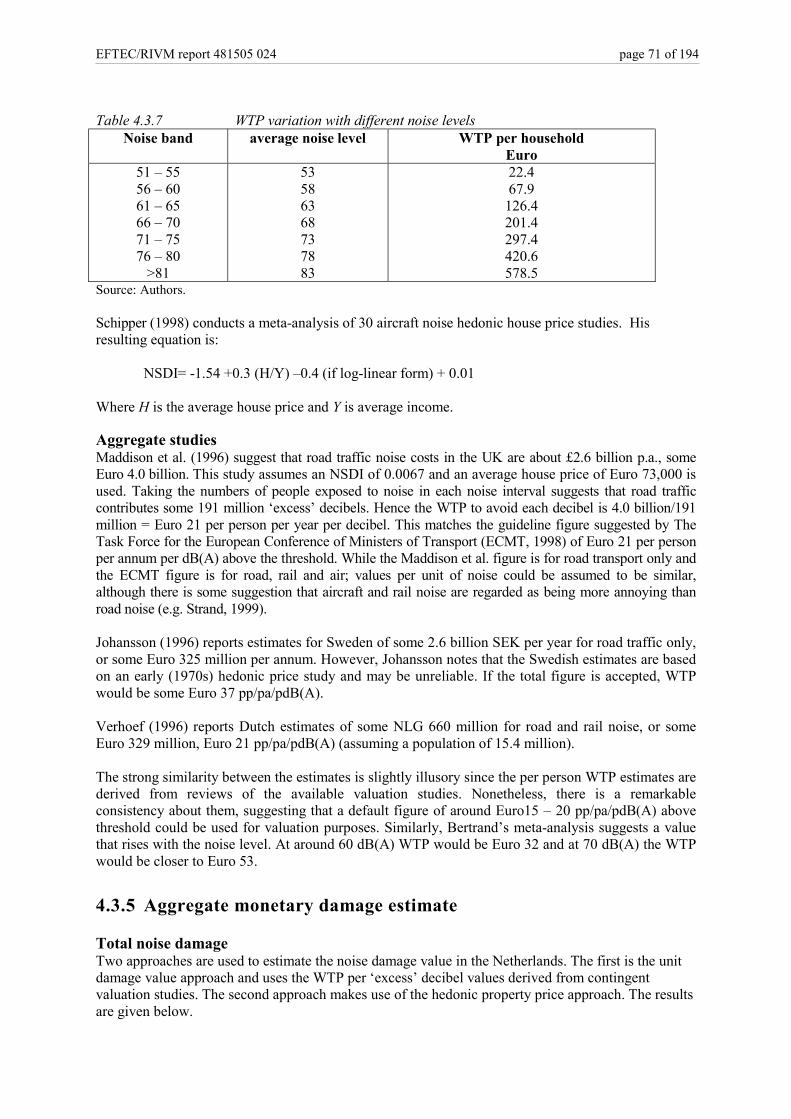
EFTEC/RIVM report 481505 024 page 71 of 194
Table 4.3.7 WTP variation with different noise levelsNoise band average noise level WTP per household
Euro51 – 5556 – 6061 – 6566 – 7071 – 7576 – 80
>81
53586368737883
22.467.9
126.4201.4297.4420.6578.5
Source: Authors.
Schipper (1998) conducts a meta-analysis of 30 aircraft noise hedonic house price studies. Hisresulting equation is:
NSDI= -1.54 +0.3 (H/Y) –0.4 (if log-linear form) + 0.01
Where H is the average house price and Y is average income.
Aggregate studiesMaddison et al. (1996) suggest that road traffic noise costs in the UK are about £2.6 billion p.a., someEuro 4.0 billion. This study assumes an NSDI of 0.0067 and an average house price of Euro 73,000 isused. Taking the numbers of people exposed to noise in each noise interval suggests that road trafficcontributes some 191 million ‘excess’ decibels. Hence the WTP to avoid each decibel is 4.0 billion/191million = Euro 21 per person per year per decibel. This matches the guideline figure suggested by TheTask Force for the European Conference of Ministers of Transport (ECMT, 1998) of Euro 21 per personper annum per dB(A) above the threshold. While the Maddison et al. figure is for road transport only andthe ECMT figure is for road, rail and air; values per unit of noise could be assumed to be similar,although there is some suggestion that aircraft and rail noise are regarded as being more annoying thanroad noise (e.g. Strand, 1999).
Johansson (1996) reports estimates for Sweden of some 2.6 billion SEK per year for road traffic only,or some Euro 325 million per annum. However, Johansson notes that the Swedish estimates are basedon an early (1970s) hedonic price study and may be unreliable. If the total figure is accepted, WTPwould be some Euro 37 pp/pa/pdB(A).
Verhoef (1996) reports Dutch estimates of some NLG 660 million for road and rail noise, or someEuro 329 million, Euro 21 pp/pa/pdB(A) (assuming a population of 15.4 million).
The strong similarity between the estimates is slightly illusory since the per person WTP estimates arederived from reviews of the available valuation studies. Nonetheless, there is a remarkableconsistency about them, suggesting that a default figure of around Euro15 – 20 pp/pa/pdB(A) abovethreshold could be used for valuation purposes. Similarly, Bertrand’s meta-analysis suggests a valuethat rises with the noise level. At around 60 dB(A) WTP would be Euro 32 and at 70 dB(A) the WTPwould be closer to Euro 53.
4.3.5 Aggregate monetary damage estimate
Total noise damageTwo approaches are used to estimate the noise damage value in the Netherlands. The first is the unitdamage value approach and uses the WTP per ‘excess’ decibel values derived from contingentvaluation studies. The second approach makes use of the hedonic property price approach. The resultsare given below.

page 72 of 194 EFTEC/RIVM report 481505 024
Unit damage value approachThe estimates of the economic value of noise nuisance presented earlier are sufficiently close that‘default’ values of a willingness to pay per person per annum per ‘excess’ decibel can be used in‘benefits transfer’ contexts. Based on the literature review presented above, we suggest that thedefault value is around Euro 20 pp/pa/pdB(A). Table 4.3.8 reports the total noise nuisance damage inthe Netherlands, based on this figure.
In 1995, noise nuisance is estimated to be Euro billion 1.6, in 2010 Euro billion 1.8, in 2020 Eurobillion 1.9 and in 2030 Euro billion 20. Noise damage is shown to be increasing between the years1995 and 2030 because there is an increasing population exposed to noise nuisance for all noise bandsbetween 56 and 80 dB(A).
Table 4.3.8 Total noise damage for the Netherlands in 1995, 2010, 2020 and 2030: Euromillion
Noise banddB(A)
Averageexceedance
Population exposedMillion
WTPEuro
Noise damageEuro million
199551-55 3 X 4.50 X 20 = 27056-60 8 X 4.17 X 20 = 66761-65 13 X 1.80 X 20 = 46866-70 18 X 0.43 X 20 = 15371-75 23 X 0.07 X 20 = 3376-80 28 X 0.02 X 20 = 9>80 32.5 X 0.00 X 20 = 1Total 1602201051-55 3 X 4.35 X 20 = 26156-60 8 X 4.57 X 20 = 73261-65 13 X 2.19 X 20 = 57066-70 18 X 0.59 X 20 = 21371-75 23 X 0.11 X 20 = 5376-80 28 X 0.02 X 20 = 13>80 32.5 X 0.00 X 20 = 2Total 1844202051-55 3 X 4.11 X 20 = 24756-60 8 X 4.70 X 20 = 75161-65 13 X 2.34 X 20 = 60866-70 18 X 0.67 X 20 = 24271-75 23 X 0.14 X 20 = 6576-80 28 X 0.02 X 20 = 14>80 32.5 X 0.01 X 20 = 4Total 1930203051-55 3 X 3.99 X 20 = 23956-60 8 X 4.85 X 20 = 77561-65 13 X 2.51 X 20 = 65266-70 18 X 0.75 X 20 = 27171-75 23 X 0.17 X 20 = 8076-80 28 X 0.03 X 20 = 16>80 32.5 X 0.01 X 20 = 4Total 2038

EFTEC/RIVM report 481505 024 page 73 of 194
Hedonic property price approachTo calculate the capital value of noise damage for the Netherlands following the hedonic propertyprice approach, we multiply the number of households exposed to average noise exceedance above50dB(A) in each noise band, by the average house price in the Netherlands and by the NSDI value.We illustrate the methodology by considering total noise (e.g. rail, road and aircraft) in theNetherlands between 1995 and 2030.
Table 4.3.9 demonstrates the total noise damage calculation for the Netherlands. For the main analysiswe assume:
• percentage population exposed to different noise bands (see table 4.3.1);
• population in the Netherlands in 1995, 2010, 2020 and 2030 assumed to be 15.4m, 16.8m, 17.7mand 18.4m respectively, (see Annex 5 on Environmental Data, Assumptions and Models);
• size of households in 1995, 2010, 2020 and 2030 is 2.34, 2.27, 2.23 and 2.21 respectively (seeAnnex 5 on Environmental Data, Assumptions and Models);
• average house price is Euro 124,921;
• NSDI is assumed to be 0.4, and
• threshold below which noise levels are not considered a nuisance is 50dB(A);
The influence of each parameter on the final result is tested in the sensitivity analysis in Section 4.3.5.

page 74 of 194 EFTEC/RIVM report 481505 024
Table 4.3.9 Total noise damage for the Netherlands in 1995, 2010, 2020 and 20301995 Noiseband
Averageexceedance
No ofhouseholds
NDSI Average houseprice
DamagePresent value
dB(A) DB(A) thousands mid Euro (2000) Euro million(2000)
51-55 3 1923 0.004 124921 2882.356-60 8 1782 0.004 124921 7122.261-65 13 770 0.004 124921 5001.166-70 18 182 0.004 124921 1636.371-75 23 31 0.004 124921 356.076-80 28 7 0.004 124921 92.2>80 32.5 1 0.004 124921 10.7TOTAL 17100.8201051-55 3 2089 0.004 124921 3131.456-60 8 2197 0.004 124921 8782.961-65 13 1054 0.004 124921 6844.966-70 18 285 0.004 124921 2559.371-75 23 55 0.004 124921 630.276-80 28 11 0.004 124921 155.5>80 32.5 1 0.004 124921 24.1TOTAL 22128.2202051-55 3 2113 0.004 124921 3167.256-60 8 2412 0.004 124921 9643.561-65 13 1201 0.004 124921 7799.366-70 18 346 0.004 124921 3107.871-75 23 72 0.004 124921 828.876-80 28 13 0.004 124921 177.4>80 32.5 3 0.004 124921 51.5TOTAL 24775.7203051-55 3 2154 0.004 124921 3228.656-60 8 2617 0.004 124921 10460.761-65 13 1353 0.004 124921 8791.466-70 18 406 0.004 124921 3655.671-75 23 94 0.004 124921 1081.676-80 28 16 0.004 124921 221.4>80 32.5 3 0.004 124921 54.1TOTAL 27493.3Note, the total damage values given in Table 4.3.9 are based on non-rounded population figures, thus the resultsmay differ if total damage is calculated based on information given in Table 4.3.9 alone.
The total cost figures presented in Table 4.3.9 are present values, these need to be annuitised to obtainan annual damage cost. We choose a 6% real annuity rate to reflect actual interest rates in the housingmarket and a lifetime of 35 years. The annuitisation factor is then 14.49. (See Definitions). The annualtotal noise cost for the Netherlands are then Euro billion 1.1 in 1995, Euro billion 1.5 in 2010, Eurobillion 1.7 in 2020 and Euro billion 1.8 in 2030 (i.e. total noise cost divided by the annuitisationfactor).

EFTEC/RIVM report 481505 024 page 75 of 194
The noise damage estimates based on the hedonic property price approach are slightly lower thanthose estimates based on the unit damage values for noise. This may be explained by the fact thatusing the hedonic price approach values noise only in the context of the home. This suggests thehedonic property price results may be biased downwards.
In order to see the level of damage caused by the different sources of noise, the following sectionsreport the noise damage estimates for road, rail and air separately based on the hedonic property priceapproach.
Road noise damage estimatesTable 4.3.10 presents the noise costs due to road traffic only according to the hedonic property priceapproach.

page 76 of 194 EFTEC/RIVM report 481505 024
Table 4.3.10 Road noise damage costs in the Netherlands: Euro million (2000), presentvalue
Noise band: dB(A) 1995 2010 2020 2030All roads51-55 2811.1 3204.7 3344.3 3479.556-60 5786.3 6922.6 7707.8 8622.961-65 3725.1 4895.4 5611.4 6400.266-70 1013.8 1606.2 2060.0 2584.471-75 128.8 255.5 428.1 650.976-80 18.4 20.7 33.3 58.3>80 0.0 0.0 0.0 0.0Present value 13483.5 16905.2 19184.9 21796.1Total annual cost 930 1166 1323 1503Highways51-55 1098.8 1363.0 1584.8 1810.356-60 1125.1 1315.2 1723.4 2190.761-65 513.8 592.1 834.0 1055.066-70 201.6 259.9 342.1 442.071-75 83.3 93.7 145.7 181.976-80 18.4 20.7 33.3 46.6>80 0.0 0.0 0.0 0.0Present value 3041 3645 4663 5726Sub-total annual cost 210 251 322 395Regional roads51-55 698.6 963.1 1140.5 1304.756-60 909.0 1267.8 1533.3 1767.961-65 745.0 1006.0 1235.5 1433.766-70 409.1 693.2 862.5 1018.871-75 22.7 119.2 218.6 335.076-80 0.0 0.0 0.0 11.7>80 0.0 0.0 0.0 0.0Present value 2784 4049 4991 5872Sub-total annual cost 192 279 344 405City roads51-55 1666.9 1932.8 2019.6 2174.956-60 3362.2 3836.0 3975.9 4271.561-65 2132.3 2859.2 3016.8 3262.366-70 326.1 573.2 748.4 996.371-75 0.0 17.0 27.3 76.676-80 0.0 0.0 0.0 0.0>80 0.0 0.0 0.0 0.0Present value 7487.4 9218.3 9788.1 10782Sub-total annual cost 516 636 675 744Note: total road noise cost values presented in Table 4.3.10, are based on the sum of the noise costs fromhighways, regional and city roads.
Road noise damage costs are estimated to be in the region of Euro billion 0.9 in 1995, Euro billion 1.1in 2010, Euro 1.3 billion in 2020 and Euro billion 1.5 in 2030. Overall road noise accounts forroughly 75% of all transport noise damage in 1995, falling to about 70% from 2010 onwards.

EFTEC/RIVM report 481505 024 page 77 of 194
Rail noise damage estimatesTable 4.3.11 presents the total rail noise damage in the Netherlands according to the hedonic propertyprice approach.
Table 4.3.11 Rail noise damage in the Netherlands: Euro million (2000), present valueNoise band: dB(A) 1995 2010 2020 203051-55 796.4 1123.0 1141.7 1143.656-60 1014.4 1415.9 1533.3 1548.161-65 770.7 1025.3 1086.2 1130.766-70 456.5 653.2 670.0 659.271-75 197.0 315.1 327.9 335.076-80 73.8 124.4 122.0 139.8>80 10.7 24.1 38.6 40.6Present value 3320 4681 4920 4997Total annual cost 229 323 339 345
Rail noise damage costs are estimated to be in the region of Euro million 200 - 300 per annum. Railnoise damage represents roughly 20% of all transport noise in the Netherlands between 1995 and2020 and this falls to 17% by 2030.
Aircraft noise damage estimatesTable 4.3.12 presents the total aircraft noise damage in the Netherlands according to the hedonicproperty price approach.
Table 4.3.12 Aircraft noise damage in the Netherlands: Euro million (2000), present valueNoise band 1995 2010 2020 2030
51-55 466.4 966.4 1097.7 1216.056-60 363.6 944.9 1207.0 1385.061-65 72.8 173.3 252.3 324.666-70 17.8 33.3 78.4 89.971-75 0.0 8.5 9.1 9.676-80 0.0 0.0 0.0 0.0>80 0.0 0.0 0.0 0.0Present value 920.6 2126.5 2644.5 3025.1Total annual cost 63 147 182 209
Aircraft noise damage in the Netherlands is estimated to be Euro million 63 in 1995, Euro million 147in 2010, Euro 182 in 2020 and Euro 209 in 2030. Aircraft noise damage represents about 5% of alltransport noise in 1995, this increases to about 10% in 2010 to 2030.
4.3.6 UncertaintyThe two main areas of uncertainty in the damage estimates for both the CVM and hedonic propertyprice are the population exposure data to noise and the assumption regarding the threshold for noise(assumed in this study as 50dB(A)). The direction of bias in the results due to the assumptionregarding the noise threshold is uncertain because some studies suggest the threshold should be nearer40dB(A), whilst others favour 55dB(A).
Results based on the unit damage approach may be an underestimate, this is mainly because of theassumption that all noise types are valued the same despite evidence that suggests aircraft and railnoise may be more 'annoying' than road noise.
The main areas of uncertainty in the results based on the hedonic property price approach are:

page 78 of 194 EFTEC/RIVM report 481505 024
- noise sensitivity depreciation index (NSDI);- average house price;- WTP per excess decibel per person per annum, and- assumption that all noise types have same impact and are given same values.
The noise damage results based on the hedonic price approach could be an underestimate this isbecause such an approach values noise only in the context of the home.
The influence of the different variables on the final result is demonstrated in the sensitivity analysisbelow.
Sensitivity analysisWe conduct a sensitivity analysis of the main areas of uncertainty, identified above. This includes:
Unit damage value approach• WTP per ‘excess’ decibel per person, per annum, based on contingent valuation approach- WTP = Euro 15 pp pa pdB(A)- WTP = Euro 20 pp pa pdB(A)- WTP = Euro 40 pp pa pdB(A)- Rising WTP with increasing noise band, see Table 4.3.7.
Hedonic property price approachSensitivities are tested against the results based on NSDI 4%, noise threshold 50dB(A), average houseprice Euro 124,921 and the population data as given in Table 4.3.2.
• lower and upper NSDI values, i.e. 0.2 - 0.7%;• noise threshold value, i.e. 55dB(A) based on Maddison et al. (1996), and• 1999 house price data.
Table 4.3.13 presents the baseline results. The ‘sensitivities’ or changes in the assumptions are thenlisted and presented with their associated quantitative effects.
Table 4.3.13 Sensitivity analysis: Euro million (2000)1995 2010 2020 2030
CLS: Annual noise damageUnit damage value approach, WTP = Euro20 pp/pa/pdB(A)
1602 1844 1930 2038
SensitivitiesWTP = Euro 15 pp /pa / pdB(A)WTP = Euro 40 pp / pa /pdB(A)WTP based on Bertrand's meta analysis(1997)See table 4.3.7
Hedonic property price approachNSDI = 0.4%, noise threshold = 50dB(A),average house price Euro 124,921,population exposure data as in table 4.3.2
(i) NSDI = 0.2%-0.7%(ii) noise threshold = 55dB(A)(iv) house price (1999) levels, Euro157,000
120132037777
1180
590 -2064503
1482
138336879639
1526
763 -2671689
1526
14473860
10471
1709
854 -2991793
1708
15284076
11401
1896
948 -3319900
1896

EFTEC/RIVM report 481505 024 page 79 of 194
From the sensitivity analysis we conclude that the results are very sensitive to the assumption of aconstant linear relationship between WTP and noise levels, i.e. compare the CLS annual noise damageresults with those derived from WTP based on Bertrand's meta analysis (1997).
We can also conclude that:
• noise damage values are highly sensitive to the choice of NSDI;
• noise damage values are highly sensitive to the choice of the noise threshold, and
• noise damages based on Eurostat (1995) average house price data are assumed to be anunderestimate due to the very low house price reported.

page 80 of 194 EFTEC/RIVM report 481505 024
4.4 Land contamination4.4.1 The issueLand is contaminated when the concentration of at least one chemical is above the intervention value,which is defined as the level of contamination above which the functioning of humans, animals andvegetation are or will be threatened and hence land may not be permitted for some uses.
4.4.2 Source of emissionsThe main categories of contaminated sites include present and former industrial sites, landfills, cardumps and gasworks. The general approach to site ‘clean-up’ is to maintain the ‘multifunctionality’ ofthe soil, i.e. maintain its potential use for various purposes, including agriculture and drinking watersupply.
This study does not address the issue of contamination of sediments in the beds of Dutch watercoursesand lakes, reported to be a major problem by OECD (1995).
4.4.3 Physical measure of impactsTable 4.4.1 shows the number of contaminated sites in the Netherlands, their distributions amongstthe land use types (1996 figures) and the distribution of land uses when all contaminated sites arecleaned. The table also shows the size (ha) of contaminated sites both for 1996 (all contaminated) andthe time when all contaminated land will be cleaned. It is assumed that on average each site is 1.8 ha.The influence this assumption has on the final result is tested in the sensitivity analysis below.
Table 4.4.1 Contaminated areasContaminated Land in 1995 Cleaned Land by 2030
No. of sites Land area (ha) No. of sites Land area (ha)Total 351,000 631,800 351,000 631,800Residential 91,228 164,210 150,000 269,993Industrial 126,328 227,390 90,768 163,384Agricultural 41,084 73,953 39,430 70,970Recreationaland nature
23,292 41,926 26,676 48,017
Derelict 29,600 53,280 4,696 8,453Dumping 7,925 14,267 2,179 3,924Other 31,540 56,774 37,248 67,046Source: RIVM, 1997 Achtergronden bij: Milieubalans 1997, Samson HD, Tjeenk Willink Alhen aan de Rijn.
Not all the sites reported in Table 4.4.1 are equally contaminated. In fact, the Dutch governmentalready has a classification scheme as follows:
60,000 sites (17% of the total contaminated sites) are ‘urgent’;116,000 sites (33% of the total contaminated sites) are ‘serious’;175,000 sites (50% of the total contaminated sites) are ‘non-serious’,Total sites = 351,000.
However, this distinction is not included in this analysis.

EFTEC/RIVM report 481505 024 page 81 of 194
4.4.4 Aggregate monetary damage estimate
Framework for analysis
Baseline current situation of contaminated land,
Full compliance all currently contaminated land areas in the Netherlands meet the nationalstandard for clean land.
By comparing the economic value of land in the Baseline scenario to the economic value of land inthe Full compliance (FC) scenario, we get an estimate of the benefits of policy measures that ensurefull compliance with national standards for clean land.
Changes in the economic value of the land use, benefit of FC scenario, arise for two main reasons, i)changes in the contamination damage within any given land use; and ii) changes in the land usecategory.
We assume that the use and value of land that currently meets the national standard for clean land isunchanged between the two scenarios and is therefore not included in the analysis.
In the analysis we consider only contaminated land. The surrounding area may also benefit from cleanup of contaminated land, this impact is difficult to measure and therefore omitted from the analysis.
Benefits of clean upBenefits of full compliance (or clean-up) can be defined as the avoided damage (or cost) ofcontamination. Benefit categories (human health, environmental quality etc) are dependent on thetype and level of contamination and the type and amount of environmental (or economic) assetswithin the contaminated area.
Box 4.4.1 presents the categories of benefits that are relevant to polluters (or private benefits) only aswell as benefits that are relevant to the society as a whole.
Box 4.4.1 Suggested benefit categories
Social benefits• Increased property values which measure the benefit to local people and which may
include the health benefits to local people,• Health benefits to visitors to the area,• Recreational benefits to local residents in so far as these are not captured in the change in
property values,• Recreational benefits to visitors to the area,• Reduced ecosystem damage not otherwise captured in recreational or property value
increase,• Gains in ‘non-use’ value, and• Gains in ‘option’ value.
Owner benefits• Increased property value,• Elimination of corporate financial environmental liability,• Elimination of potential for litigation / prosecution,• Positive public relations value and avoidance of negative public relations, and• Protection of a resource used as a key input to the problem holder’s production process.

page 82 of 194 EFTEC/RIVM report 481505 024
Measurement of benefitsOwner benefits are reflected in the land value. It is not possible to measure the social benefits, due tolack of full scientific understanding of the effects of contamination of soils and the site-specific natureof the effects that are understood. Despite this shortfall, land values may include some social benefits,unfortunately it is not possible to determine which social benefits, nor their size. This suggests thatchange in land value is a conservative estimate of the benefits of clean up.
The present value of benefit of clean up is equivalent to the sum of all land value changes due to cleanup. This value will be different for agricultural, residential and industrial / commercial land use typesand can be measured by the sale value of land based on the currently available records and views ofestate agents, e.g. average price per ha of agricultural land, average value of private housing perhectare.
Application of methodologyStage 1: estimate economic value of land in the Baseline:1 Identify total land area currently defined ‘contaminated’ ( LB)
Table 4.4.12 Define current land use (i) for land areas defined 'contaminated' i.e. agriculture,
housing, industry / commercial, wildlife, derelict. (LB = ΣΣΣΣ Li)Table 4.4.1
3 Identify average land use value for contaminated land, i.e. value for agriculture,housing, industry etc, (Euro per hectare) Note that property values must also be Euro/ ha, (Pi)We assume the value for derelict and dumping land is zero.For the baseline calculations it is assumed that the price of contaminated land is10%less than the price of clean land with all other characteristics remaining the same.For sensitivity analysis, it is assumed that the price reduction due to contamination is5%.
4 Calculate baseline total value of contaminated land (BLD = ΣΣΣΣ Pi . Li)Table 4.4.2
Stage 2: estimate economic value of land in the FC5 Assume contaminated land area is now cleaned to a ‘clean’ state, LS
Table 4.4.16 Determine possible new land uses (j) for land areas cleaned to a ‘clean’ state.
Where (LS = ΣΣΣΣLj).Table 4.4.1
7 Identify average land use value for ‘clean’ land, i.e. value for agriculture, housing,industry etc, (Euro per hectare) (we assume value of ‘clean’ land is the same asvalue of land that has never been contaminated, i.e. full price) Property values mustalso be Euro / ha (Pj)Residential (average of raw lot and ready for building) = Euro607,620/haIndustrial (firms) = Euro586,300/haAgricultural = Euro21,320/haRecreational and nature = Euro5,330/haDerelict and dumping assumed to be zero‘Other’ is assumed to equal industrial = Euro586,300/ha
8 Calculate total value of previously contaminated land now cleaned, i.e.(FCD = ΣΣΣΣ Pj x Lj)Table 4.4.2
Stage 3: estimate benefit of FC9 Compare land use value in baseline to land use value in FC, i.e. benefit of FC = FCD
- BLD.Estimates are present values. Table 4.4.2

EFTEC/RIVM report 481505 024 page 83 of 194
Table 4.4.2 presents the results of Stage 2 above, where it is assumed that price of contaminated landis 10% less than the price of equivalent clean land17. It is also assumed that all contaminated land iscleaned.
Table 4.4.2 Benefits of full clean-up PV: Euro million (2000 prices)Residential 74254Industrial -24195Agricultural 94Recreational and nature 55Derelict 0Dumping 0Other 9351TOTAL 59559Annual value overinfinity
3371
The benefits are determined by two main factors:• change in the value of land, i.e. 10% increase, and• change in the distribution of the land uses within the contaminated area. The shift is towards
residential from other uses. Given that residential area has the highest value, the large magnitudefor the benefits of clean-up is reached.
4.4.5 UncertaintyThe main areas of uncertainty in estimating the benefits of cleaning contaminated land are as follows:
• number of contaminated sites: the estimate given in Table 4.4.1 is probably an underestimate ofthe current situation. When all potentially contaminated sites are examined (in 2005), it is likelythat the total number of sites will increase 1.5 times.
• conversion of ‘number of contaminated sites’ to size of contaminated land: the average area of acontaminated site (1.8ha) is probably an overestimate. This figures could be closer to 0.94 ha for‘urgent’ locations and 0.22 ha for serious locations.
• value of clean land is clearly very much dependent on the location. However, such differencescannot be well represented by the average values used;
• value of contaminated land: According to guidelines for real-estate agencies prices are influencedby contamination in five different ways. These are: cost of clean up (and who has to pay for theclean up), limitations of the use possibilities, inconvenience, negative image of the surroundingsand uncertainty. The cost of clean up are subtracted from the price as long as the owner of theland has to pay for the clean up. This means that when the government pays for the clean upoperation there are no costs subtracted. When the costs of clean up are for the owner it isimportant to realise that the value of the land can not be negative. So when the costs of clean upare higher than the value of the land, the value will be zero. For the limitations of the use valuethere is a subtraction of 5% of the value of the property for houses with a garden. This is becausethere are limitations in using the garden. There are no subtractions when the land is usedindustrial. Inconvenience occurs during the clean up operations and therefore 10% of the value issubtracted for residential and industrial use. This subtraction can even be 20% if theinconvenience is extreme. It is important to realise that the percentages are percentages of the
17 The value of contaminated land at 10% less than uncontaminated land supported by the on going work byEFTEC and others for the Canadian Council of Ministers to the Environment (CCME) and the UK EnvironmentAgency.

page 84 of 194 EFTEC/RIVM report 481505 024
total estate value, thus not only the land value but also the buildings on the contaminated land.The negative image of the surrounding has to be concluded from market development becausethis is different for each location. This is also the case for uncertainty. In other words foruncertainty and negative image no general estimations can be done. In general it can be said thatthe value of contaminated land highly depends on the location and that it is hard to make generalestimates. Because in the past the government did the clean up, there were no transactions ofcontaminated land. Another problem is that the Dutch housing and industrial offices market isvery tight, so it is hard to draw conclusions from the market situation. The only real informationthat is available is the 5% and 10% subtraction of the property value, as mentioned above.
Overall, the uncertainty of the damage estimates for land contamination in the Netherlands is great.The presence of large uncertainty makes it all the more essential that benefits analysis of landcontamination is conducted in future, it serves to both expand knowledge in the area and reduceuncertainty and act as a signal to the Netherlands to collect more relevant data.
Sensitivity analysis1. The value of contaminated land is 5% less than the value of clean land (baseline assumption is 10%
difference);
2. The average area of a contaminated site is 0.58 ha (average of 0.22 and 0.94 ha as mentioned above)(baseline assumption is 1.8 ha per site);
3. Average area of a contaminated site is 0.58ha and the value of contaminated land is 5% less than thevalue of clean land.
The results of the above sensitivity analyses are presented in Table 4.4.3.
Table 4.4.3 Sensitivity analysis: PV: Euro million (2000 prices), annuity at 6%1 2 3
Residential 69265 23927 22320Industrial -30861* -7796* -9944*Agricultural 15 30 5Recreational and nature 44 18 14Derelict 0 0 0Dumping 0 0 0Other 7687 3014 2477TOTAL 46150 19193 14872Annual value overinfinity
2612 1086 842
* net cost of clean up.
Sensitivity analysis above confirms the importance of the magnitude of the value and size of land. Italso shows that both in baseline and sensitivity analysis, clean-up of industrial land (given theassumptions explained above) results in a net cost. It is mainly because due to the high value and areaof residential land that clean-up generates net benefits on the whole.
Given the degree of uncertainty associated with the assumptions made in the above analysis, weconsider the results for this problem are less certain than the results for the other environmental issues.The assumptions reflect the site-specific nature of the problem rather than an inherent uncertainty inthe methodology. In other words, if the same exercise were done for a given site (rather than thewhole country), the results would be significantly more robust.

EFTEC/RIVM report 481505 024 page 85 of 194
4.5 Particulate matter4.5.1 The issueSuspended particulate matter (PM) is made up of a variety of materials and discrete objects and maybe liquid or solid, organic or inorganic. PM makes up most of the visible and obvious form of airpollution and is a contributor to summer and winter smogs characteristic of urban areas. Pollutantparticles vary in size, from 0.001 µm to 10 µm; small solid particles include carbon black, silveriodide, combustion nuclei and sea salt nuclei. Large particles include cement dust, wind blown soildust, foundry dust and pulverized coal. Liquid particulate matter or mist, includes raindrops, fog andsulphuric acid mist. Particles of organic origin include viruses, bacteria and spores. The mostimmediate effect of particles is loss of visibility but particulate matter also influences weather and airpollution phenomena by providing active surface on which heterogeneous atmospheric reactions canoccur.
Air pollution can affect human health by damaging the respiratory tract directly or by entering theblood or lymph systems. Soluble particulate matter can also be transported to organs some distancefrom the lungs. A strong correlation has been found between increases in the daily mortality rate andacute episodes of air pollution. Damage may also occur to buildings, historic monuments andvegetation near or within cities.
4.5.2 Source of emissionsParticles are commonly suspended in the air near the sources of pollution, such as the urbanatmosphere, industrial plants, highways, and power plants. The major sources of particulate matter innon-industrial urban areas, are from coal and wood heating and road transport burning diesel fuel. Inindustrial cities, the main source of particulate matter is power generation.
4.5.3 Physical measure of impacts
Population at riskThe main environmental impacts of particulate matter are the ill-health effects, such as prematuremortality and morbidity.
Current legislation scenario: emissions and impactsThe data for impacts associated with exposure to PM10 are drawn from the NEO5 (draft report), usingthe medium scenario (EC). The emissions data for PM10 are presented in Table 4.5.1, whilst Table4.5.2 gives the premature mortality and morbidity cases per annum. The dose / exposure responsefunctions used to establish the human health effects are given in full in the Appendix to this chapter.
Table 4.5.1 PM10 emissions: 1000 tonnes1990 2010 2020 2030
Consumers 6.8 6.5 6.6 6.7Energy sector 0.6 0.4 0.3 0.3Industry 14.3 7.9 8.2 8.4Other 1.3 0.7 0.7 0.2Refineries 4.8 2.0 1.8 1.8Transport 18.6 9.9 9.8 11.0TOTAAL 46.4 27.5 27.4 28.4Source: NEO5 (draft report).
It is important to note that not all particulate matter is of ‘anthropogenic’ origin. Some arises as anatural background level (e.g. dust) and is not generally subject to policy measures. This studyconsiders the impact of particulate matter of 'anthropogenic' origin only.

page 86 of 194 EFTEC/RIVM report 481505 024
Table 4.5.2 Mortality and morbidity effects due to PM10
Mortality (number of people)1995 2010 2020 2030
Total 931 992 1172 1529Aged under 65 135 147 152 142Aged 65+ 796 845 1020 1387Morbidity (number of unscheduled hospital admissions)TotalCOPDAsthmaCardiovascular disease
23049581331214
2315953122
1240
28661161129
1576
35001401136
1963Source: NEO5 (draft report).
Air pollution-related mortality affects largely the elderly, in this study we see that 88% of prematuredeaths are in the over 65 group. Note that total mortality in Table 4.5.2 is restricted to mortalitycaused by cardiovascular disease, COPD and pneumonia18. Also note that the morbidity data arerestricted to unscheduled hospital admissions for three impacts: COPD, asthma and cardiovasculardisease. Exposure to PM10 causes other morbidity impacts, which do not result in hospitalisation butwhich nevertheless should be valued for a complete picture of morbidity effects resulting from PM10.Data are unavailable for the incidence of other morbidity effects, however the sensitivity analysis inthe final section explores the effect of different possible assumptions with regard to morbidity.
Particulate matter also has effects on visibility, this is not included in the benefits assessment due tothe lack of valuation work in this area.
4.5.4 Monetary measure of impactDamage estimates due to particulate matter are measured in terms of number of premature deaths andunscheduled ill-health incidences. We can interpret the damage estimates as a measure of the potentialbenefits that could be secured due to the introduction of measures that control particulate matter,where benefits are understood to be the avoided deaths and ill-health incidences.
Human healthValuation of morbidity impacts to human health are undertaken using the sum of three values: (i)willingness to pay to avoid each type of episode of ill-health, (ii) productivity loss to employers, and(iii) health care costs of treatment for emergency room visits and hospital admissions, where these arerelevant. These values are specific to the Netherlands, and are taken from CSERGE et al., 1999.
Premature mortality impacts are valued using a value of statistical life (VOSL) of Euro million 3.47 in2000 prices. However, as noted above particulate-related premature mortality affects largely theelderly (over 85% of premature deaths are in the over 65 group). There is some evidence that valuesof risk aversion are lower for this age group at around 70% of the prevailing risk values (see Pearce1998). This reduces the VOSL to Euro million 2.4 (2000 prices). The unit values used to value allhealth impacts are presented in Table 4.5.3.
18 In the Fifth National Environmental Outlook total mortality is defined as all deaths excluding accidents etc.
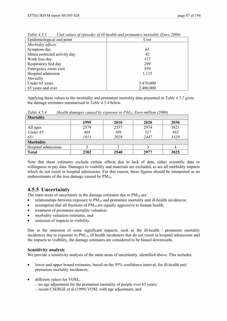
EFTEC/RIVM report 481505 024 page 87 of 194
Table 4.5.3 Unit values of episodes of ill-health and premature mortality (Euro 2000)Epidemiological end point CostMorbidity effectsSymptom dayMinor restricted activity dayWork loss dayRespiratory bed dayEmergency room visitHospital admissionMortalityUnder 65 years65 years and over
6142
117299559
1,115
3,470,0002,400,000
Applying these values to the morbidity and premature mortality data presented in Table 4.5.2 givesthe damage estimates summarised in Table 4.5.4 below.
Table 4.5.4 Health damages caused by exposure to PM10: Euro million (2000)Mortality
1995 2010 2020 2030All agesUnder 6565+
23794681911
2537509
2028
2974527
2447
3821492
3329MorbidityHospital admissions 3 3 3 4Total 2382 2540 2977 3825
Note that these estimates exclude certain effects due to lack of data, either scientific data orwillingness to pay data. Damages to visibility and materials are excluded, as are all morbidity impactswhich do not result in hospital admissions. For this reason, these figures should be interpreted as anunderestimate of the true damage caused by PM10.
4.5.5 UncertaintyThe main areas of uncertainty in the damage estimates due to PM10 are:• relationships between exposure to PM10 and premature mortality and ill-health incidences;• assumption that all fractions of PM10 are equally aggressive to human health;• treatment of premature mortality valuation• morbidity valuation estimates, and• omission of impacts to visibility.
Due to the omission of some significant impacts, such as the ill-health / premature mortalityincidences due to exposure to PM2.5, ill health incidences that do not result in hospital admissions andthe impacts to visibility, the damage estimates are considered to be biased downwards.
Sensitivity analysisWe provide a sensitivity analysis of the main areas of uncertainty, identified above. This includes:
• lower and upper bound estimates, based on the 95% confidence interval, for ill-health andpremature mortality incidences;
• different values for VOSL;- no age adjustment for the premature mortality of people over 65 years;- recent CSERGE et al (1999) VOSL with age adjustment, and

page 88 of 194 EFTEC/RIVM report 481505 024
- recent CSERGE et al (1999) VOSL without age adjustment.
• different morbidity valuations, based on ExternE values.
Table 4.5.5 presents the adopted assumptions and the baseline results derived. The ‘sensitivities’ orchanges in the assumptions are then listed and presented with their associated quantitative effects.
Table 4.5.5 Sensitivity analysis: Euro million (2000)Adopted assumption: premature mortalityPremature mortality (mean estimate) valued with VOSL: Euro million 3.47 for people under 65 yearsand Euro million 2.4 for those over 65 years.
1995 2010 2020 2030Current legislation scenarioestimate mean 2382 2540 2977 3825Sensitivities• no age adjustment• CSERGE VOSL age adjusted• CSERGE VOSL no age
adjustment
323134154637
344036794937
406543155834
530455467612
lower upper lower upper lower upper lower upperBaseline estimate (lower, upper) 79 6770 81 7147 93 8389 125 10523Sensitivities• no age adjustment• CSERGE VOSL age adjusted• CSERGE VOSL no age
adjustment
102107146
906593151300
9
111117159
95641036013726
127134183
11336
12160
16269
175181251
144701527020760
Adopted assumption: morbidityMorbidity valued based on CSERGE et al (1999)Baseline estimate 4 4 5 6Sensitivity• ExternE values 32 32 39 47
lower upper lower upper lower upper lower upperBaseline estimate (lower, upper) 1.6 6.9 1.6 6.9 2.0 8.1 2.5 9.7Sensitivity• ExternE values 12.7 54.8 12.8 64.9 16.0 64.9 19.7 77.3
We conclude from the sensitivity analysis the following:
• health damage estimates are highly sensitive to the statistical relationships between exposure toPM10 and ill-health and premature mortality incidences;
• health damage estimates due to PM10 are sensitive to the manner in which premature mortality isvalued and to a lesser extent the approach to morbidity valuation.

EFTEC/RIVM report 481505 024 page 89 of 194
Appendix Dose / exposure response functions used
Health Effects
Dose / exposure response functions used in the modelling exerciseThe dose-response functions given here are specific to the Netherlands, they are higher than thosedose-response functions typically used elsewhere.
Table 4.5.6 Dose-response functions used in this modelling exerciseMortality: relative riskRelative risk associated with a 80 µg/m3 change in the 24h average PM10 concentration (and 95%confidence interval)
Age All causes Cardiovascular COPD Pneumonia<45 0.927
(0.844 - 1.018)0.906
(0.728 - 1.128)1.153
(0.587 - 2.268)1.427
(0.806 - 2.525)45-64 1.008
(0.964 - 1.053)1.023
(0.945 - 1.106)1.139
(0.841 - 1.541)1.712
(1.042 - 2.815)65-74 1.017
(0.979 - 1.056)1.002
(0.945 - 1.062)1.166
(0.991 - 1.372)1.240
(0.879 - 1.748)75+ 1.030
(1.006 - 1.055)1.016
(0.981 - 1.052)1.066
(0.965 - 1.178)1.123
(1.011 - 1.247)all ages 1.021
(1.002 - 1.040)1.012
(0.984 - 1.041)1.099
(1.015 - 1.191)1.148
(1.040 - 1.268)Morbidity Emergency hospital admissionsRR for a 80 µg/m3 change in the 24h average PM10 concentration (and 95% confidence interval)
All respiratorydiseases
Chronicobstructivepulmonary
disease
Asthma Cardiovascular Diseases
<15 0.939(0.896 - 0.984)
0.922(0.799 - 1.064)
0.895(0.794 - 1.010)
-
15-64 1.063(1.015 - 1.113)
1.120(1.029 - 1.219)
1.140(1.000 - 1.299)
1.001(0.970 - 1.034)
65+ 1.078(1.035 - 1.121)
1.160(1.096 - 1.227)
1.125(0.897 - 1.409)
1.038(1.012 - 1.064)
all ages 1.027(0.998 - 1.056)
1.111(1.061 - 1.164)
0.995(0.914 - 1.083)
1.022(1.001 - 1.043)
Source: daily mortalitiy (acute) from Hoek et al. tables 16a-d, 16i en 19a-d. Morbidity dose response functionsare from Vonk and Schouten tables 20a-d.
For comparison, the dose-response functions used in ExternE (1997) are given in Table 4.5.7. Thesehave not been used in the sensitivity analysis due to the complexity of the modelling exercise.However, they are provided here for transparency and comparison.
Table 4.5.7 Dose-response functions used elsewhere in the literatureHealth impact Coefficient SourceAcute mortality 0.04% Spix and Wichmann, 1996RHAs (all population) 2.07 x 10⁻⁶ Ponce de Leon et al., 1996Cerebrovascular hospitaladmission
5.04 x 10⁻⁶
RADs (all population) 0.025 Ostro and Rothschild, 1989Source: ExternE National Implementation the Netherlands, IVM (1997).

page 90 of 194 EFTEC/RIVM report 481505 024
4.6 Eutrophication4.6.1 The issueThe process of eutrophication is caused by nutrient imbalances, which disturb the natural biochemicalbalance of ecosystems. In particular eutrophication restricts the intentional uses of water-bodies overlarge areas. The nutrients of particular concern are nitrogen (from ammonia and nitrate) andphosphorous. The enrichment of natural waters by nutrients, primarily nitrogen in marine waters, butalso phosphorous in low salinity waters, has been associated with increased primary productivity andnuisance algal growth in the coastal zones and semi-enclosed areas of seas. The consequences of thiscan be increased frequency of algal blooms (sometimes toxic), increased water turbidity, slimeproduction, oxygen depletion in deep waters and mass fish and benthic fauna kills. The issue ofcontaminated groundwater and its health aspects to humans is also a cause of wide concern.
4.6.2 Source of emissionsDomestic sources dominate nitrogen emissions, accounting for approximately 63% of total emissions.This is followed by agriculture (11%) then industrial sources and atmospheric depositions in roughlyequal proportions (10% each). The major sources of phosphorous emissions are domestic (e.g.washing powders) and industrial sources, each accounting for approximately 45% of emissions.
4.6.3 Physical measure of impacts
Current legislation scenario: emissionsThe data for nitrogen and phosphorous emissions are drawn from the NEO5 (draft report), using themedium scenario (‘EC’). These are reported in Table 4.6.1. Table 4.6.1 also gives the sectoralbreakdown of emissions for each pollutant.
It is important to note that these emissions relate only to emissions from sources within theNetherlands. The Netherlands is also likely to be affected by emissions from other Europeancountries, for example emissions into surface waters which flow into the Netherlands. Unfortunately,however, data on emissions from other European countries which affect the Netherlands are notavailable.
The receiving environment is obviously of relevance for the valuation of these emissions.Unfortunately, at this point the existing data are not available at a very disaggregated level. However,RIVM have indicated that approximately 50% of nitrogen is emitted to ‘regional waters’, defined asditches, small streams, small canals, with the remainder emitted to ‘large waters’, i.e. rivers, largecanals, lakes etc. For phosphorous, approximately 30% to 40% of emissions are to regional waters.

EFTEC/RIVM report 481505 024 page 91 of 194
Table 4.6.1 Nitrogen and phosphorus emissions: current legislation scenarioN (thousand tonnes)
1996 2010 2020 2030Total emissions 56 33 33 33Domestic effluent 35.06 21.84 22.81 23.46Agriculture 6.27 0.92 0 0Industry 5.70 3.80 3.80 3.80Atmospheric deposition 5.62 4.21 4.01 3.88Sewage 1.20 0.98 0.93 0.88Overflow 1.09 0.97 0.88 0.87Households not connected 0.69 0.23 0.23 0.23P (thousand tonnes)Total emissions 7.6 3.5 3.6 3.6Industry 3.55 0.66 0.66 0.66Domestic effluent 3.36 2.64 2.73 2.80Overflow 0.12 0.09 0.11 0.11Households not connected 0.11 0.07 0.07 0.07Agriculture 0.44 0.03 0.01 0.00Source: NEO5 (draft report)
4.6.4 Monetary measure of impactsThere is a lack of reliable dose-response functions describing the relationships between nitrates,phosphorus and eutrophication. Therefore in order to value the impact of eutrophication it is necessaryto consider people’s willingness to pay to improve water quality in general.
There is a significant literature on valuation of changes to water quality, which is summarised inTable 4.6.2.
Table 4.6.2 Nitrogen and phosphorus emissions: current legislation scenarioStudy Location Valuation basis Valuation
(Euro2000) River water quality Green andTurnstall(1991)
UK WTP for improvement in water quality toRE3WTP for improvement in water quality >RE3
0.94/person/visit 1.10/person/visit
MiddlesexUniversity(1994)
UK Non-use value for improvements in waterquality• from very poor to moderate• from moderate to good coarse fishery• from good coarse fishery to trout• from trout to salmon fishery
223,900/km/yr 24,100/km/yr 27,600/km/yr 5,500/km/yr
Hanley(1989)
UK Guarantee of water supplies with nitratelevels not exceeding 50mg/l
26.66/hh/year
Lant andRoberts(1990)
USA improvements from poor to fair water quality• recreational value• 'intrinsic' value
39pp.pa 49pp.pa

page 92 of 194 EFTEC/RIVM report 481505 024
Table 4.6.2 (ctd) Nitrogen and phosphorus emissions: current legislation scenarioGreen andWillis(1996)
UK WTP of anglers for improvements in waterquality• new relatively poor coarse fishery• new good coarse fishery• new good trout fishery Non-use value for improvements in quality• from poor to medium• from medium to good
6.23/angler/visit 9.95/angler/visit 26.13/angler/vst 0.0087/hh/km/yr 0.0033/hh/km/yr
Reservoir Pearson(1992)
UK Maintain water quality at a standard highenough to support boating and recreationalactivities
30.20/hh/year
Coastal waters Machado etal. (1998)
Portugal Mean WTP for improvements to ‘acceptable’levels of water quality
10.83/person/visit
Georgiou etal. (1998)
UK Mean WTP to ensure that EC bathing waterstandards are met• Great Yarmouth• Lowestoft
18.60/hh/yr20.60/hh/yr
Feenbergand Mills(1980)
USA –Bostonbeaches
WTP for a 10% beach water qualityimprovement (indicators: oil, total bacteria,colour)
3.50pp.pa(beach users)
Bockstaelet al.(1987)
USA –Bostonbeaches
� WTP of users for a 10% beach waterquality improvement (indicators: oil, FC,COD)
� WTP of users for a 30% beach waterquality improvement (indicators: oil,turbidity, FC, COD)
� 11.46 pp.pa� 0.57 pp/visit
� 36 pp.pa� 1.50 pp/visit
Bockstaelet al.(1989)
USA –ChesapeakeBay
WTP for an improvement from‘unacceptable’ to ‘acceptable’ beach waterquality
147 pp.pa (beach users)
McConnelland Ducci(1989)
Barbadosbeaches
WTP for sewerage reduction 10 – 165 pp.pa
McConnelland Ducci(1989)
Uruguaybeaches
WTP for sewerage reduction to improvewater quality to swimming levels
13 pp.pa
Choe et al.(1996)
Philippinebeach
WTP for sewerage reduction to improvewater quality to swimming levels
11 – 22 pp.pa
Georgiou etal. (1996)
UKbeaches
Improvement of water quality to meet ECstandards
18 – 69 pp.pa
One major research project has conducted extensive valuation studies of eutrophication in the Baltic Sea(Turner et al., 1995, 1997). The study involved several contingent valuation and travel cost studies in thecontext of an assumed 50% nutrient load reduction programme which can legitimately be regarded as a‘maximum feasible reduction’ scenario since such a programme has substantial costs of nearly Eurobillion 4 per annum. The results are set out in Table 4.6.3. The Polish CVM studies involved a beachsurvey (Zylicz, 1995a) and a household survey, with, in each case, respondents being asked their WTP

EFTEC/RIVM report 481505 024 page 93 of 194
for clean-up programme (Zylicz, 1995b). The first two surveys give very close results, but the surprisingfeature is the sheer size of the WTP figures. Taking the Swedish results as being typical of the westEuropean economies and the Polish results as being typical of the EITs, Turner et al. (1997) estimateBaltic basin wide benefits from a clean-up programme to be some SEK69 billion per year, or some Eurobillion 8.0 per annum compared to costs of Euro billion 3.6 pa. If non-respondents are treated as havingimplicit zero WTP for the clean up programme, then benefits reduce to SEK billion 37.9 per annum orabout Euro billion 4.4: benefits are still greater than costs though by a fairly narrow margin.
Table 4.6.3 Median Willingness to Pay to Improve the State of the Baltic Sea (2000 Euro)Study Country WTP % Income
Zylicz et al., 1995aBeach survey, CVM
Poland 62 – 116 pp.pa 3-5%
Zylicz et al., 1995bhousehold survey, CVM
Poland 28 – 69 pp.pa 1.3-3.3%
Mail survey, CVM Poland 99 – 200 pp.pa 4.6-9.5%Sandstrøm, 1995, TCMbeach use
Sweden 30 per trip
Søderqvist, 1995, CVM Sweden 315 pp.pa
Total N and P loads to the ‘Baltic proper’ (the geographical zone used in the study) in 1993 were860,000 tN and 33,000 tP per year (Turner et al., 1995). Based on the total benefit of 50% reductionin this load, Table 4.6.4 presents the benefits per unit of N and P.
Table 4.6.4 Benefits of nitrogen reduction in the Baltic Sea (Euro/tonne)Pollutant Euro/tonne
NP
11,03011,120
Source: Authors.
The difficulty in transferring the values produced in any of the above studies to value eutrophicationof inland waterways in the Netherlands is threefold, these are:
First, the valuation studies in existence tend to estimate WTP for a given improvement in waterquality. It is difficult to estimate the relationship between a change in emissions and a change inwater quality since this is highly dependent on the receiving environment. While it might be possibleto estimate the relationship on a site-specific basis, it is evidently a much more complex task at anational level.
Second, willingness to pay for water quality improvements will depend on both the existing waterquality, and the proposed improvements. There is no satisfactory data available concerning theexisting water quality of inland and coastal waters in the Netherlands at the sort of level of detailrequired for this analysis. Site-specific characteristics of the water body will also be relevant, forexample the extent to which it is used for recreational and commercial purposes, whether it is urban orrural, its ‘uniqueness’ in terms of biological or other functions. It is possible to adjust for thesefactors on a local scale, when considering changes to a single water resource. However, it becomesmuch more difficult when considering the national water resources as a whole.
Finally, all of the valuation studies to date have examined WTP for a change to a given waterresource. It is generally accepted that WTP for improvements is dependent on the existence of othersimilar resources (‘substitute resources’) nearby. Therefore, even if data were available on existingwater quality, possible improvements linked to emissions reductions, and site-specific characteristics

page 94 of 194 EFTEC/RIVM report 481505 024
for all water bodies in the Netherlands, it is not clear that aggregation of WTP for improvements overall water bodies would be valid.
Another possible approach is to use the cost of clean-up for these pollutants as a measure of damagesi.e. the cost of controlling discharges is used as a proxy for the damage done by the discharges. Theanalytical foundations of this approach are far less robust, since it effectively means that control costsequal damage costs, implying that the ratio of benefits to costs of control are always unity. In addition,clean-up cost will vary depending on the technology used. These results should therefore be viewed assupplementary to the WTP results. If the pollutants are actually removed in the treatment process, thencost of clean-up is a true estimate of the damage caused. However, if they are not removed, thenwillingness to pay estimates are the correct measures of damage.
For the purposes of estimating clean-up costs, it is assumed that the treatment is chosen so that the treatedsewage meets the relevant standards across Europe, which are assumed to be based on correctassumptions regarding the assimilative capacity of the receiving environment. A paper by Odegaard(1996) gives the efficiency of each sewage treatment in terms of expected removals of specific nutrients(including total P-phosphate, total N) and the costs of these treatments. The ‘best’ method is ‘advancedtertiary’, using chemical/biological means which remove 95% BOD, 90% total P and 70% total N at acost of 3.11 NKr/m3 (0.34 Euro/m3). More usefully, the cost is given as a cost/efficiency factor, at a costper kilogram removed. The results are given in Table 4.6.5 below.
Table 4.6.5 Cost-efficiency factors for chemical and biological pollutants: post-DN, pre-precipPollutant % removed NKr/tonne Euro/tonne removed
Total N 70 112,000 15,000Total P 90 562,000 74,000
For the purposes of the damage assessment, both the cost of clean-up values and the WTP data areused, in order to give a range of possible values for this environmental problem. It should be notedthat these values are only indicative of the likely magnitude of the problem, for all of the reasonsdiscussed above.
4.6.5 Aggregate monetary damage estimateCombining the emissions data of Section 4.6.3 with the valuation estimates in Section 4.6.4, thedamage estimates given in Table 4.6.6 below are obtained.
Table 4.6.6 Damages due to nitrogen and phosphorus emissions (million Euro)
1996 2010 2020 2030
N 618 - 840 364 - 495 364 - 495 364 - 495P 85 - 562 39 - 259 40 - 266 40 - 266Total 702 - 1,402 403 - 754 404 - 761 404 - 761Note: lower values assume WTP, upper values assume ‘costs of clean up’.
4.6.6 UncertaintyThe main sources of uncertainty are due to the scientific data with respect to the water quality in theNetherlands and the lack of evidence of a WTP for a reduction of eutrophication impacts for inlandwaters in the Netherlands.
Due to the lack of information regarding the issue of eutrophication we are unable to conduct ameaningful sensitivity analysis.

EFTEC/RIVM report 481505 024 page 95 of 194
In order to assess eutrophication in the Netherlands in the future it could require an originalcontingent valuation survey asking respondents for their WTP for an increase in their local waterquality as well as a maximum WTP to increase water quality for all waters in the Netherlands. Theresults of such an analysis could then be aggregated across the Netherlands in order to establish theoverall damage due to eutrophication.

page 96 of 194 EFTEC/RIVM report 481505 024
4.7 Low level ozone4.7.1 The IssueLow level ozone is caused by emissions of nitrogen oxides and volatile organic compounds reactingin sunlight. Generally low level ozone concentrations are higher during the day and in the summer.However, the issue of estimating the effects of low level ozone is further complicated because it formsover time and may be worse in rural areas downwind of significant sources of emissions. Low levelozone is considered to cause harm to humans via the respiratory organs and the eyes. Ozone alsocauses damage to vegetation and crops in and around urban areas.
4.7.2 Source of emissionsLow level ozone is a secondary pollutant caused by the interaction of the precursors, nitrogen oxides,NOx, and volatile organic compounds VOCs, in the presence of sunlight. SOx and NH3 are alsoimplicated. Low level ozone is often called photochemical smog or just smog. Due to the role ofsunlight, the concentrations of low level ozone are generally higher during the day and in the summer.
Motor vehicles account for a considerable proportion of the total emissions of nitrogen oxides inEurope, and their contribution is expected to increase following the growth in use of the private car.The main source of VOCs is from the combustion of petrol and diesel in urban areas. Other sourcesinclude the burning of coal or wood for heating, solvents and industry.
4.7.3 Physical measure of impactsEstimating damages from low level ozone is complex because it forms over time and may be worse inrural areas downwind of significant sources of emission. Tropospheric ozone is implicated in theforms of damage summarised in Table 4.7.1.
Table 4.7.1 Environmental impacts of low-level ozoneReceptor ImpactHuman health Mortality;
Respiratory hospital admissions;Restricted activity days;Symptom days;
Crops Reduced yield;Forests Reduction in tree growth;
Non-crop vegetation damage, andMaterials Damage to some materials (paints, plastics, rubbers, metals).
Rabl and Eyre (1997) suggest that while the effect of ozone to materials is potentially significant, it islikely to be small. Thus, low level ozone damage to materials is excluded. Low level ozone is knownto reduce tree growth. However, there is currently very little information about the damage to forestsdue to the complexity of their growth and management systems. Similarly, while it is likely that ozonecauses damage to ecosystems, there are very few studies estimating these effects. Thus ozone damageto forests and biodiversity are also excluded from this study.
Effects on human health and crops are analysed below. Recommended D/ERFs for both human healtheffects and effects on crops are given in full in the Appendix to this chapter.
Current legislation scenario: emissions and impactsThe data for the precursor pollutants are drawn from the NEO5 (draft report), using the mediumscenario (‘EC’). The emissions data for NOx are presented in Table 4.2.2 in Section 4.2. Data onVOC emissions are drawn from the same source and are presented in Table 4.7.2 below. Table 4.7.2also gives the sectoral breakdown for VOCs.
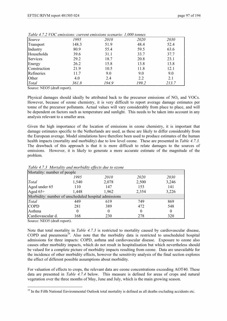
EFTEC/RIVM report 481505 024 page 97 of 194
Table 4.7.2 VOC emissions: current emissions scenario: 1,000 tonnesSource 1995 2010 2020 2030Transport 148.3 51.9 48.4 52.4Industry 80.9 55.4 59.5 63.6Households 39.6 31.1 33.7 37.7Services 29.2 18.7 20.8 23.1Energy 26.2 15.8 13.8 13.8Construction 21.9 10.5 11.8 12.1Refineries 11.7 9.0 9.0 9.0Other 4.0 2.4 2.2 2.1Total 361.8 194.9 199.2 213.7Source: NEO5 (draft report).
Physical damages should ideally be attributed back to the precursor emissions of NOx and VOCs.However, because of ozone chemistry, it is very difficult to report average damage estimates pertonne of the precursor pollutants. Actual values will vary considerably from place to place, and willbe dependent on factors such as temperature and sunlight. This needs to be taken into account in anyanalysis relevant to a smaller area.
Given the high importance of the location of emissions in ozone chemistry, it is important thatdamage estimates specific to the Netherlands are used, as these are likely to differ considerably fromthe European average. Model simulations have therefore been used to produce estimates of the humanhealth impacts (mortality and morbidity) due to low level ozone. These are presented in Table 4.7.3.The drawback of this approach is that it is more difficult to relate damages to the sources ofemissions. However, it is likely to generate a more accurate estimate of the magnitude of theproblem.
Table 4.7.3 Mortality and morbidity effects due to ozoneMortality: number of people
1995 2010 2020 2030Total 1,540 2,078 2,500 3,246Aged under 65 110 147 153 141Aged 65+ 1,448 1,962 2,354 3,226Morbidity: number of unscheduled hospital admissionsTotal 449 619 749 869COPD 281 389 472 548Asthma 0 0 0 0Cardiovascular d. 168 230 278 320Source: NEO5 (draft report).
Note that total mortality in Table 4.7.3 is restricted to mortality caused by cardiovascular disease,COPD and pneumonia19. Also note that the morbidity data is restricted to unscheduled hospitaladmissions for three impacts: COPD, asthma and cardiovascular disease. Exposure to ozone alsocauses other morbidity impacts, which do not result in hospitalisation but which nevertheless shouldbe valued for a complete picture of morbidity impacts resulting from ozone. Data are unavailable forthe incidence of other morbidity effects, however the sensitivity analysis of the final section exploresthe effect of different possible assumptions about morbidity.
For valuation of effects to crops, the relevant data are ozone concentrations exceeding AOT40. Thesedata are presented in Table 4.7.4 below. This measure is defined for areas of crops and naturalvegetation over the three months of May, June and July, which is the main growing season.
19 In the Fifth National Environmental Outlook total mortality is defined as all deaths excluding accidents etc.

page 98 of 194 EFTEC/RIVM report 481505 024
Table 4.7.4 Ozone concentrations exceeding AOT40: ppm.hour1995 2010 2020 2030
AOT40 sum averaged over Dutch agricultural area 7.5 – 9.1 7.5 – 9.1 7.1 – 8.6 7.1 – 8.6
4.7.4 Monetary measure of impacts
Human HealthValuation of morbidity impacts to human health is undertaken using the sum of three values: (i)willingness to pay to avoid each type of episode of morbidity, (ii) productivity loss to employers, and(iii) health care costs of treatment for emergency room visits and hospital admissions, where these arerelevant. These values are specific to the Netherlands, and are taken from CSERGE et al., (1999).
Premature mortality impacts are valued using a VOSL of 3.47 million Euro, adjusted to 2.4 millionEuro for people aged over 65. The basis of VOSL value is explained in Annex A3 on Valuing Risk ofPremature Mortality. The unit values used to value all health impacts are presented in Table 4.7.5below.
Table 4.7.5 Total costs of episodes of ill-health: Euro (2000)Epidemiological End Point CostMorbidity effectsSymptom day 61Minor restricted activity day 42Work loss day 117Respiratory bed day 299Emergency room visit 559Hospital admission 1,115MortalityUnder 65 years 3,470,00065 years and over 2,400,000
Applying these values to the morbidity data presented in Table 4.7.3 gives the damage estimatessummarised in Table 4.7.6 below.
Table 4.7.6 Health damages caused by low-level ozone: million Euro (2000)1995 2010 2020 2030
MortalityAll ages 3,858 5,218 6,182 8,232under 65 383 509 532 48965+ 3,475 4,709 5,651 7,743MorbidityHospital admissions 0.5 0.7 0.8 0.9Total 3856 5219 6183 8233
CropsCrop damage due to exposure to ozone levels is a function of ozone dose, crop species, cultivar,biological conditions, climatic conditions, soil conditions, production and other factors. Interaction ofthese variables makes accurate crop loss assessment especially difficult over large areas. Theestimates provided below are a first order approximation of crop damage in the Netherlands due tolow level ozone.
Ozone is considered to cause yield reduction for ‘ozone sensitive’ crops. Jones et al. (1997) list thesecrops as summarised in Table 4.7.7.

EFTEC/RIVM report 481505 024 page 99 of 194
Table 4.7.7 Ozone sensitive cropsSlightly
Sensitive CropsSensitive
CropsVery
SensitiveCrops
milletoats
pasture grassricerye
sorghum
applesbeanscarrotsclover
cucumbersdatesflax
grapefruitgrapeshemp
hopslemonslimes
linseedmelons
oil seedsonionsorangespeaches
pears
plumspotato
rape seedsesame seeds
soybeanssunflowertangerines
tomatowatermelons
wheat
Tobacco
Production levels for the relevant crops in the Netherlands are taken from the FAO StatisticalDatabase online. These are presented in the Appendix to this chapter. The reduction in yields causedby exposure to ozone is valued at world prices, also taken from the FAO Statistical Database. Theserepresent the true value of crops and are unaffected by market distortions such as subsidies under theCommon Agricultural Policy which tend to affect prices significantly.
To obtain an estimate of total damages to crops from low-level ozone, the ozone concentration datagiven in Table 4.7.4 have been used in conjunction with the dose response functions listed in theannex plus the FAO production and price data for the crops above. Total damages to crops aresummarised in Table 4.7.8 below.
Table 4.7.8 Crop losses caused by low-level ozone: million Euro (2000)1995 2010 2020 2030
All crops 169 – 205 169 – 205 160 – 194 160 – 194
A recent Dutch study, (Tenneijck et al., 1998) supports the crop damage estimates in Table 4.7.8. TheDutch study estimates the benefits to the Netherlands in terms of avoided crop damage due to a 70%reduction of 1995 low level ozone concentrations is about Euro 200 million per annum.
The above analysis of crop damage due to ozone exposure is a first order approximation of the truedamage. The analysis assumes constant crop prices, even though with reduced ozone levelsproduction could increase forcing prices down. We also assume that the crop mix through timeremains the same despite the decrease in ozone emissions. It is likely, that as ozone levels fall therecould be a significant reduction in the production of ozone tolerant crops because of the reducedprofitability relative to crops that were more sensitive to ozone.
4.7.5 Aggregate monetary damage estimateAggregating the damages to human health (mortality and morbidity) and the crop losses estimated inSection 4.7.4 above, gives estimates of total damages caused by low-level ozone as summarised inTable 4.7.9 below.

page 100 of 194 EFTEC/RIVM report 481505 024
Table 4.7.9 Total damages caused by low-level ozone: million Euro (2000)1995 2010 2020 2030
Human healthMortality (all ages) 3,858 5,218 6,182 8,232Under 65 383 509 532 48965+ 3,475 4,709 5,651 7,743Morbidity:Hospital admissions 0.5 0.7 0.8 0.9Crop lossesAll crops 169 – 205 169 – 205 160 – 194 160 – 194Total
All costs 4,028 – 4,064 5,388 – 5,424 6,343 – 6,377 8,393 – 8,427
Note that these estimates exclude certain effects due to lack of data, either scientific data orwillingness to pay data. Damages to materials, forests and ecosystems are all excluded, as are allmorbidity impacts which do not result in hospital admissions. For this reason, these figures should beinterpreted as an underestimate of the true damage caused by low-level ozone.
Damages due to ozone in the Netherlands are expected to increase over time, from Euro 4.1 billion in1995 to over Euro 8 billion in 2030. This, however, is due to the changing age structure of thepopulation in the Netherlands, which has a growing proportion of the population in the over 65 agegroups. The health impacts of ozone affect the elderly disproportionately, and the health impactsaccount for by far the largest proportion of total damages. Actual ozone concentrations in the countryare expected to decrease during the time frame under consideration.
It should be noted that the estimates presented here are restricted to the ozone problem as perceivedby the population of the Netherlands. In other words, some of the ozone formation in the Netherlandswill be due to the emissions of NOx and VOCs from other countries. Also, the emissions of NOx andVOCs in the Netherlands will tend to contribute to ozone formation outside the country, this damageis not accounted for in the current estimates.
4.7.6 UncertaintyThe main sources of uncertainty in this analysis are:
• approach to premature mortality;• omission of impacts to materials, forests, ecosystems, non-crop vegetation and biodiversity.
Ozone is known to damage some polymeric materials such as paints, plastics and rubbers as wellas having a corrosive effect on metals. However, ExternE (CEC, 1995) suggests that furtherresearch is necessary before these impacts can be quantified. Similarly, recent evidence suggestsozone is the primary cause of damage to forests and that it causes damage to ecosystems. Theseeffects have all been omitted from the analysis due to uncertainty in both the scientific andeconomic valuation estimates. Their exclusion will tend to bias the results downward;
• morbidity effects other than hospital admissions – i.e. emergency room visits, symptom days and‘restricted activity days’. All of these are known to be linked to ozone, however, at the time ofwriting, data on their incidence in the Netherlands were not available, and
• dose-response functions for crops do not take into account of changing farm practices that reducethe susceptibility of crops to ozone.
Overall, the damage estimates for low level ozone may be biased downwards due to the omission of anumber of potentially important impacts.

EFTEC/RIVM report 481505 024 page 101 of 194
The sensitivities considered are as follows:
1. Effect of assuming different values for a VOSL. The valuation of mortality effects is conductedusing a ‘value of statistical life’. For more details on this approach see Annex 3 on valuing therisk of premature mortality. Mortality incidence in the over 65 age group is valued at 70% of aVOSL, based on the results of Pearce (1997). The sensitivity explores three different assumptionsabout the value of a VOSL, namely:
• the effect of removing the age adjustment;• using the latest VOSL estimate by CSERGE et al (1999) with age adjustment, and• using the CSERGE estimate without age adjustment.
2. Effects of adopting older unit value estimates for valuation of morbidity effects: The baselineresults are based on the latest unit damage estimates from CSERGE et al. (1999). These are themost up-to-date estimates of WTP to avoid these impacts, and are also specific to the Netherlands.For these reasons, the damage estimates produced are likely to be much more accurate thanprevious estimates. However, most cost-benefit assessments to date have been based on adifferent set of unit values, adjusted from American studies. These are summarised in Annex 4 onMonetary Valuation of Health Effects. Therefore, for purposes of comparison of our results withprevious studies, we explore the effect of using the older set of estimates.
The results of these sensitivities are presented in Table 4.7.10 below.
Table 4.7.10 Sensitivity analysis: million Euro (2000)1995 2010 2020 2030
Mortality costsCurrent legislation scenarioestimate 3,858 5,218 6,182 8,232Sensitivities:(i) No age adjustment 5,407 7,317 8,701 11,684(ii) CSERGE value ageadjusted
5,603 7,578 8,980 11,961
(iii) CSERGE no ageadjustment
7,760 10,501 12,488 16,769
Morbidity costsHospital admissions - baseline 0.5 0.7 0.8 0.9Sensitivities:(i) ExternE values 4.0 5.5 6.6 7.7
Finally, one more sensitivity is conducted based on the scientific uncertainty surrounding themorbidity and mortality impacts:
Upper and lower bounds due to scientific uncertainty: The 95% confidence intervals for mortality andmorbidity incidence resulting from the scientific analysis has been combined with the baselineassumptions, and the sensitivities outlined above, to produce an overall range of estimates. Table4.7.11 presents the results.

page 102 of 194 EFTEC/RIVM report 481505 024
Table 4.7.11 Sensitivity- mortality and morbidity effects due to ozone (million Euro)1995 2010 2020 2030
Mortality costslower upper Lower upper lower upper lower upper
Baseline 2,231 6,628 3,030 8,845 3,615 10,499 4,987 13,416Sensitivities:(i) No age adjustment 3,221 9,063 4,375 12,113 5,221 14,477 7,205 18,747(ii) CSERGE value ageadjusted
3,244 9,615 4,405 12,833 5,257 15,238 7,252 19,482
(iii) CSERGE no ageadjustment
4,622 13,007 6,278 17,384 7,493 20,777 10,341 26,905
Morbidity costsHospital admissions: baseline 0.0 1.7 0.1 2.2 0.1 2.6 0.1 3.0Sensitivities:(i) ExternE values 0.1 14.3 0.5 18.1 0.6 21.7 0.7 24.9

EFTEC/RIVM report 481505 024 page 103 of 194
Appendix Dose / exposure response functions assumed
Health Effects
Dose / exposure response functions used in the modelling exerciseThe dose-response functions given here are specific to the Netherlands, and are higher than thosedose-response functions typically used elsewhere.
Table 4.7.12 Dose-response functions used in this modelling exerciseAcute mortality:Relative risk associated with a 150 µg/m3 change in the 8h average Ozone concentrationbetween 12:00-20:00 (and 95% confidence interval)
Age All causes Cardiovascular COPD Pneumonia
<45 0.983(0916 - 1.054)
1.022(0.863 - 1.212)
2.137(1.258 - 3.630)
1.142(0.682 - 1.911)
45-64 1.040(1.004 - 1.077)
1.038(0.977 - 1.103)
1.083(0.856 - 1.371)
0.677(0.424 - 1.081)
65-74 1.030(1.0 - 1.061)
1.005(0.960 -1.053)
0.989(0.862 - 1.135)
1.597(1.164 - 2.190)
75+ 1.043(1.024 - 1.063)
1.073(1.044 - 1.102)
0.996(0.919 - 1.079)
1.367(1.245 - 1.501)
All ages 1.039(1.024 - 1.054)
1.055(1.032 - 1.079)
1.006(0.942 - 1.074)
1.146(1.062 - 1.236)
Morbidity: emergency hospital admissionsCoefficient for a 150 µg/m3 change in the 8h average Ozone concentration between 12:00-20:00(and 95% confidence interval)
Age All respiratorydiseases
COPD Asthma Cardio vasculardiseases
<15 0.954(0.913 - 0.997)
0.838(0.731 - 0.960)
0.918(0.834 - 1.010)
-
15-64 1.023(0.985 - 1.061)
0.925 9 0.855 - 1.001)
1.096(0.990 - 1.203)
0.993(0.970 - 1.018)
65+ 1.045(1.008 - 1.082)
1.115(1.054 - 1.179)
1.051(0.897 - 1.231)
1.010 (0.990 - 1.029)
All ages 1.017(0.992 - 1.042)
1.034(0.989 - 1.082)
1.029(0.968 - 1.094)
1.002(0.986 - 1.018)
Source: daily mortality from Hoek et al. Tables 16a-d, 16i en 19a-d. Relative risk for morbidity from Vonk andSchouten tables 20a-d.
For comparison, the dose-response functions used in ExternE (1997) are given in Table 4.7.13. Thesehave not been used in the sensitivity analysis due to the complexity of the modelling exercise.However, they are provided here for transparency and comparison.
Table 4.7.13 Dose-response functions used elsewhere in the literatureHealth impact Coefficient SourceAcute mortality 0.059%* Sunyer et al.,1996RHAs (all population) 7.09 x 10⁻⁶ Ponce de Leon et al., 1996Symptom days (allpopulation)
0.033 Krupnick et al., 1990
RADs (all population) 9.76 x 10⁻³ Ostro and Rothschild, 1989Source: ExternE National Implementation the Netherlands, IVM (1997)

page 104 of 194 EFTEC/RIVM report 481505 024
The exposure response coefficients presented in Table 4.7.13 are for Western Europe and has units of(cases / year-person-µg/m3) for morbidity and (% change in annual mortality rate/µg/m3) formortality.
Further information on the unit values used for the valuation of morbidity and mortality effects can befound in Annex 4 on Monetary Valuation of Health Effects since these effects are common to severalpollutants.
CropsJones et al (1997) reviews the effects of air pollution on crops and reports the dose response functionsreproduced in Table 4.7.14.
Table 4.7.14 Physical measure of the effects of ozone on cropsType of crop Dose-response functionTolerant cropsSlightly sensitive cropsSensitive cropsVery sensitive crops
0% loss in yields per ppm hour AOT401.0% loss in yields per ppm hour AOT401.75% loss in yields per ppm hour AOT403.57% loss in yields per ppm hour AOT40
The problems with these DRFs include:� the omission of farmer adaptation, and� part of damage that is accounted for by plant adaptation. Ozone concentrations are highest on hot
dry days and there is evidence to suggest that plants protect themselves on such days to conservemoisture. This protection also has the effect of protecting against damage from ozone.
These effects are difficult to quantify. However, both would suggest that the use of the dose-responsefactors given in Table 4.7.14 without adjustment to account for these effect would result in anoverestimate of the effects of ozone on crops. However, without further information on the likelymagnitude of this effect, it is impossible to quantify in the estimates presented here.
In order to estimate the effects on production, and the value of crop losses, production and price datafor these crops in the Netherlands was taken from the FAO Statistical Database. These are presentedin Table 4.7.15.

EFTEC/RIVM report 481505 024 page 105 of 194
Table 4.7.15 Crop Production in the Netherlands and Prices (1995)Type of crop Production (Mt) Price (1990 $US/Mt)
Slightly sensitive cropsRye 42,500 107Oats 15,500 109
Sensitive CropsApples 560,000 307Beans, Dry 5,000 539Beans, Green 72,800 427Carrots 368,900 163Cucumbers and Gherkins 506,500 223Flax Fibre and Tow 34,000 961Grapes 300* 340Linseed 6,000 267Onions, Dry 438,600 202Peaches and Nectarines 12* 369Pears 140,000 335Plums 6,600 309Potatoes 7,340,000 110Rapeseed 5,000 328Tomatoes 560,700* 192Wheat 1,167,000 144* data from 1994 since 1995 data not available,Source: FAO Statistical Database.
Materials damageOzone is known to damage some polymeric materials such as paints, plastics and rubbers as well ashaving a corrosive effect on metals (Lee et al., 1995). However, ExternE (CEC, 1995) suggests thatfurther research is necessary before these impacts can be quantified. The UN ECE Programme (Kucera,1994) states that the corrosive effect of ozone on metals is very uncertain, but recent evidence shows thatozone is probably important in accelerating some reactions. Kucera (1994) shows that ozone also actssynergistically with SO2 especially for zinc. Although zinc is not an important construction material, it isused extensively as a protective coating for steel.
The DRFs in the existing literature are presented in Table 4.7.16 below. These have not, however,been used in the current analysis due to the uncertainty surrounding these estimates, and the lack of ameasure of ‘stock at risk’ for the Netherlands. They are presented here for completeness.
Table 4.7.16 Dose-response functions for the effect of ozone on zincType of zinc Dose-response function
(mass loss after 4 years (g/m2))Unsheltered zinc 14.5 + 0.043 x TOW x SO2 x O3 + 0.08 x H+
Sheltered zinc 5.5 + 0.013 x TOW x SO2 x O3TOW is the time of wetness and H+ is a measure of acidity (meq/m2/year).Source: Kucera (1994).
Forest damageOzone is the primary cause of damage to forests. At the UNECE Kuopio workshop, the following twodose-response functions were proposed for ozone effects on forest productivity:

page 106 of 194 EFTEC/RIVM report 481505 024
Beech: % productivity change = -0.27xNorway spruce: % productivity change = -0.18x
Where, x is the ozone expressed as AOT40, that is the ozone concentration accumulated over athreshold of 40ppb in daylight hours over the growing season, expressed in ppm.hours. However,there is a high level of uncertainty associated with there two functions, which increases in theextrapolation from two species to all deciduous and coniferous species, and to the whole of Europe(AEA, 1998a). This is compounded by difficulties in monetary valuation. Due to the high levels ofuncertainty with these results, valuation of forest damages is not estimated here.
Ecosystem damageSimilarly, while it is likely that ozone causes damage to ecosystems, there are very few studiesestimating these effects. They have therefore been omitted from the current analysis.

EFTEC/RIVM report 481505 024 page 107 of 194
4.8 Damage assessment and priority issues4.8.1 Ranking environmental issues according to damage estimatesRanking environmental issues is useful in the sense of highlighting priority issues and pointing outany surprises, for example, noise nuisance is a priority issue, whereas acidification is becoming less ofan environmental problem than it used to be. Such exercises can be used for awareness raising fordecision makers. However, ranking alone does not answer any questions about policy. In order to doso we would need to compare the benefits of environmental control with the costs, the unit damagevalues used in this benefit assessment study can be re-used if a CBA is conducted in future.
Table 4.8.1 summarises the damage assessment results for the various environmental issues in theNetherlands. They are the mean per annum damage estimates and at this stage they are not discounted(with the exception of the damage estimates for land contamination, which are present values of totaldamage). All values are in Euro (2000 prices).
Table 4.8.1 Total annual damages: not discounted: Euro million, (2000 prices)1995 2010 2020 2030
Climate change 1942 1948 2064 2234Acidification 2647 - 2975 1459 - 1631 1437 - 1610 1516 - 1700PM10 2382 2540 2977 3825Eutrophication 702 - 1402 403 - 754 404 - 761 404 - 761Low level ozone 4028 - 4064 5388 - 5424 6343 - 6377 8393 - 8427Noise 1602 1844 1930 2038Land contaminationPresent value 59559
Due to the existence of international treaties for the control of climate change and acidification, theclimate change estimates are damages to the world due to greenhouse gases from the Netherlands, andfor acidification the estimates are damages to the UNECE due to acidifying pollutant emissions fromthe Netherlands. Note that the land contamination damage estimates are present values.
In order to prioritise the environmental issues in order of damages (or mean potential primary benefitsfrom control), the damage estimates must be made directly comparable. This is complicated by thefact that damage estimates for land contamination are already present values. In order to include theland contamination damage assessment in the comparison with the other environmental issues weconvert all damage estimates into present values (discount rate = 6%). Table 4.8.2 gives the totaldamage estimates as a present value as well as the corresponding annual damage value (for therelevant formulas refer to Definitions). It is now possible to compare and rank the environmentalissues in the Netherlands in terms of greatest potential primary benefits from control. Table 4.8.2gives the ranking.
Table 4.8.2 Total and annual damage estimates for environmental issues in the Netherlandstotal damage (mid)
present value discount rate=6%Euro million (2000)
Annual damage (mid)
Euro million (2000)
Ranking Qualitativeassessment
Low level ozone 110034 - 110613 6228 - 6261 1 ++Land contamination 59559 3371 2 --PM10 54471 3083 3 ++Acidification 37017 - 41569 2095 - 2353 4 ++Climate change 36766 2081 5 ++Noise 31980 1810 6 +Eutrophication 9835 - 19224 557 - 1088 7 --Note: the annual damage values assume a linear distribution of benefits between 1995-2030.
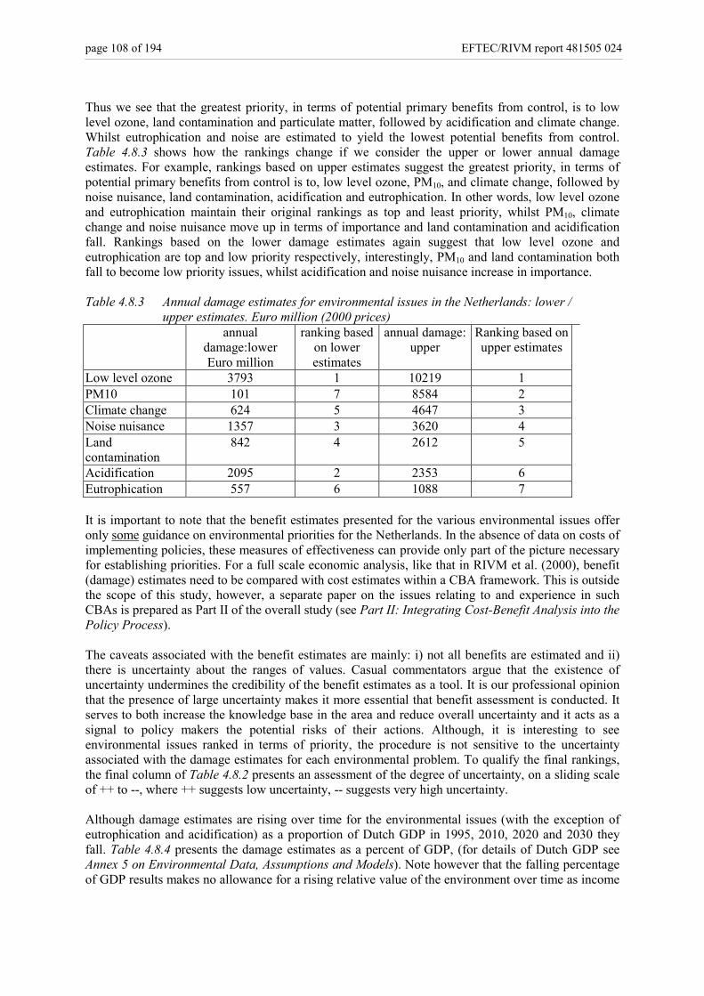
page 108 of 194 EFTEC/RIVM report 481505 024
Thus we see that the greatest priority, in terms of potential primary benefits from control, is to lowlevel ozone, land contamination and particulate matter, followed by acidification and climate change.Whilst eutrophication and noise are estimated to yield the lowest potential benefits from control.Table 4.8.3 shows how the rankings change if we consider the upper or lower annual damageestimates. For example, rankings based on upper estimates suggest the greatest priority, in terms ofpotential primary benefits from control is to, low level ozone, PM10, and climate change, followed bynoise nuisance, land contamination, acidification and eutrophication. In other words, low level ozoneand eutrophication maintain their original rankings as top and least priority, whilst PM10, climatechange and noise nuisance move up in terms of importance and land contamination and acidificationfall. Rankings based on the lower damage estimates again suggest that low level ozone andeutrophication are top and low priority respectively, interestingly, PM10 and land contamination bothfall to become low priority issues, whilst acidification and noise nuisance increase in importance.
Table 4.8.3 Annual damage estimates for environmental issues in the Netherlands: lower /upper estimates. Euro million (2000 prices)
annualdamage:lowerEuro million
ranking basedon lowerestimates
annual damage:upper
Ranking based onupper estimates
Low level ozone 3793 1 10219 1PM10 101 7 8584 2Climate change 624 5 4647 3Noise nuisance 1357 3 3620 4Landcontamination
842 4 2612 5
Acidification 2095 2 2353 6Eutrophication 557 6 1088 7
It is important to note that the benefit estimates presented for the various environmental issues offeronly some guidance on environmental priorities for the Netherlands. In the absence of data on costs ofimplementing policies, these measures of effectiveness can provide only part of the picture necessaryfor establishing priorities. For a full scale economic analysis, like that in RIVM et al. (2000), benefit(damage) estimates need to be compared with cost estimates within a CBA framework. This is outsidethe scope of this study, however, a separate paper on the issues relating to and experience in suchCBAs is prepared as Part II of the overall study (see Part II: Integrating Cost-Benefit Analysis into thePolicy Process).
The caveats associated with the benefit estimates are mainly: i) not all benefits are estimated and ii)there is uncertainty about the ranges of values. Casual commentators argue that the existence ofuncertainty undermines the credibility of the benefit estimates as a tool. It is our professional opinionthat the presence of large uncertainty makes it more essential that benefit assessment is conducted. Itserves to both increase the knowledge base in the area and reduce overall uncertainty and it acts as asignal to policy makers the potential risks of their actions. Although, it is interesting to seeenvironmental issues ranked in terms of priority, the procedure is not sensitive to the uncertaintyassociated with the damage estimates for each environmental problem. To qualify the final rankings,the final column of Table 4.8.2 presents an assessment of the degree of uncertainty, on a sliding scaleof ++ to --, where ++ suggests low uncertainty, -- suggests very high uncertainty.
Although damage estimates are rising over time for the environmental issues (with the exception ofeutrophication and acidification) as a proportion of Dutch GDP in 1995, 2010, 2020 and 2030 theyfall. Table 4.8.4 presents the damage estimates as a percent of GDP, (for details of Dutch GDP seeAnnex 5 on Environmental Data, Assumptions and Models). Note however that the falling percentageof GDP results makes no allowance for a rising relative value of the environment over time as income

EFTEC/RIVM report 481505 024 page 109 of 194
rises. If these relative valuations rise at the same rates as GDP, the proportion of damage to GDPwould remain the same.
Table 4.8.4 Environmental damage estimates as a percent of Dutch GDP: %1995 2010 2020 2030
Low level ozone 1.32 1.12 1.01 1.02PM10 0.76 0.53 0.47 0.46Climate change 0.62 0.40 0.33 0.27Acidification 0.85 - 0.95 0.30 - 0.34 0.23 - 0.25 0.18 - 0.20Eutrophication 0.22 – 0.45 0.08 – 0.16 0.06 – 0.12 0.05 – 0.09Noise 0.51 0.38 0.30 0.25Total 4.29 - 4.62 2.82 - 2.93 2.40 - 2.48 2.22 - 2.29
Table 4.8.4 suggests that environmental damage in the Netherlands was a significant proportion ofGDP in 1995, ranging from 1.3% for low level ozone, between 0.6% and0.8% for PM10, climatechange and acidification, to roughly 0.5% for noise and eutrophication. Overall, total environmentaldamage due to low level ozone, PM10, climate change, acidification, eutrophication and noise isestimated to be roughly 4.5% GDP in 1995, falling to about 2% in 2030. It is interesting to comparethese figures with the estimates of expenditure on pollution abatement, reported to be about 1.2% ofGDP in 1990 (ERECO, 1992).
4.8.2 Burden of disease associated with selected environmentalexposures
IntroductionTo describe and compare the disease burden associated with environmental exposures, and,eventually, to perform cost effectiveness analysis of options for environmental policy. Some sort of‘public health currency’ is required. Considering the fact that annual mortality or even loss of lifeexpectancy does not fully represent the environmental health loss, we tentatively applied an approachlargely based on the ‘burden of disease’ measure that was developed by Murray and Lopez on behalfof the World Bank and WHO (1995). To assess the global disease burden, and consequently thehealth policy priorities in different regions in the world, they employed ‘disability adjusted life years’(DALYs). This health impact measure combines years of life lost and years lived with disease ordisability that are standardised by means of severity weights, (World Bank, 1999 and Murray andLopez, 1996). The notion that the multiform health loss due to environmental exposure is fairly wellcharacterised by three dominant aspects of public health, viz. quantity of life (life expectancy), qualityof life, and social magnitude or number of people affected inspired our adaptation of the DALY-concept. Provisional calculations for the Netherlands indicated that the contribution of environmentalexposures to the total disease burden would probably not exceed 3%, which is roughly equivalentwith the burden caused by car accidents, Hollander et al. (1999).
Figure 4.1 sketches the basic idea behind our approach. At birth potentially each of us may expectaround eighty years of healthy life. However, our genetic program, our often-unfavourable life-styles,poverty, occupational or environmental conditions or just bad luck, means most of us will encounterdisease that will reduce the quality of part of our life. These diseases may manifest themselves inepisodes, chronic or even progressive until death. Some of us will die abruptly, for instance caused byan accident or an infectious disease. Thus, public health loss is defined as time spent with reducedquality of life, aggregated over the population involved. The methodology to estimate burden ofdisease associated with environmental exposures is described elsewhere (see Hollander et al., 1999).

page 110 of 194 EFTEC/RIVM report 481505 024
CalculationsIn the framework of the 5th National Environmental Outlook adequate data and future projections areonly available for particulate matter, tropospheric ozone, noise, UV, radon, home dampness and foodborne infectious disease. For each relevant health outcome we calculated attributable risks bycombining population weighted exposure distributions with relative risk estimates derived from theepidemiological literature. Subsequently for each health outcome the number of cases was estimatedby combining baseline incidence rates with the attributive risks. Calculations of future disease burdenare based on projections of future population structure. Table 4.8.5 presents the set of endpoints weused to arrive at estimates of attributable disease burden and the number of DALYs lost. Finally atotal exposure attributable disease burden was calculated by aggregating the number of DALYs foreach health outcome. The disease burden associated with additional UV-exposure due to ozone layerdegradation was calculated by aggregating annual morbidity and mortality estimates of skin cancerand Dutch burden of disease data (Melse et al., 2000). Statistical uncertainty was assessed usingMonteCarlo techniques.
Table 4.8.5 Disability-Adjusted Life Years (DALYs) per 1000cases lost to air pollution and UV-radiation.
5-95%-tile(mean)
Environmental factor Health outcomeParticulate air pollution Mortality 55-830Short-term - respiratory
- coronary heart dis- pneumonia- otherhospital admission- respiratory 11-34- cardiovascular 12-36emergency room visits- respiratory 3.5-33.5aggravation of asthma 0.1-1.0- asthmatic attacks- use of bronchodilatorsaggravation of resp. symptoms- upper respiratory. Tract 0-1.8- lower respiratory. Tract 1-15affected lung function- decreased FEV1 >10% 0
Ozone Mortality 55-830- respiratory- cardiovascular- pneumonia- otherhospital admission- respiratory disease 11-34emergency room visits- respiratory disease 11-34
UV-A/UV-B Mortality 24,000 (mean)O3-layer degradation Melanoma
OtherMorbidityMelanoma 650-1200basal cell 4-17squamous cell 58-190

EFTEC/RIVM report 481505 024 page 111 of 194
Indoor radon Mortalitylung cancer 13,500Morbiditylung cancer 640-1150
Home dampness MorbidityAsthma 45-112chronic respiratory symptoms 10-74
Noise Mortality 11.000 (mean)CardiovascularMorbidityHypertensionacute myocardial infarctionangina pectoris 200-350cerebrovascular disease 500-720
Food borne infectiousdisease
Mortality 13,500 (mean)
- Campylobacter spp. Complications- Salmonella spp. Morbidity 1.9-3.8- SRSV gastro-enteritis- E. coli (VTEC 0157) Guillain-Barré syndrome- toxin producing reactive arthritis(C. perfigens, B. cereus) haemolytic uraemic syndrome (HUS)
FindingsFigure 4.2 shows the annual disease burden for 2000, and 2030 (for the European Co-ordinationscenario, in some cases 2020). The health effects of air pollution (particulates, andat some distance, troposheric ozone) dominate the disease burden associated with the set ofenvironmental exposures. The future disease burden is to a large extent the result of future changes inthe population structure (higher share of elderly people that are affected by this type of air pollution).Another environmental issue associated with a high disease burden is noise exposure (both from roadand air traffic). We refrained from attributing disease burden to the large number of people reportingserious annoyance and sleep disturbance. There is much discussion whether these responses should beregarded as a damage to human health or rather as (merely) a social response. Instead we estimatedthe possible fraction of cardiovascular disease attributable to noise exposure based on the results ofseveral large epidemiological studies implicating a causal association. Disease burden caused bychemicals (heavy metals, PAHs and benzene) is relatively minor (and is not presented in the figure).The contribution of UV radiation also appears to be relatively minor (however, attributive diseaseburden will rapidly increase until after 2050 due to a large time lag).
The figure also shows the estimates for indoor problems (radon and home dampness) and food borneinfectious disease. Although the disease burden is high, it is questionable if these problems can beconsidered as environmental and are subject to environmental policies. However, the estimates can beused as reference points. The findings suggest that the disease burden associated with air pollution(particulate matter and tropospheric ozone) and noise exposure are substantial. Future policiesfocusing on these issues may yield a fair public health benefit for 2030.
Uncertainties and caveatsIt has to be noted that the estimates for health effects of air pollution and noise are based on the resultsof epidemiological studies involving serious methodological problems (e.g. borderline resolution,confounding, external validity). Attributable disease burden numbers should be considered asmaximum impact estimates.

page 112 of 194 EFTEC/RIVM report 481505 024
It is important to note that attributable disease burden is only one of the many aspects that characteriseenvironmental risk. Other aspects that determine the social acceptability of environmental risk arevoluntariness of exposure, equity of the distribution of risks and benefits, trust in risk managers andgovernment, and perceived controllability. Catastrophic potential is another important attribute:several studies have shown that accident that victimise a large number of people at the same time,such as aircraft or nuclear accidents, are much less accepted than accidents that kill small numbers ofpeople a time, e.g. traffic accidents. The social disruption that takes place in response to largeaccidents may justify putting more weight on potential victims of nuclear accidents than on thefaceless victims of air pollution or UV radiation.
Comparison with monetary benefit results: robustness testThe results of the damage assessment methodology presented in the earlier parts of Chapter 4 andsummarised in Tables 4.8.1, 4.8.2 and 4.8.3 are in support of those derived from the DALY analysis.Both approaches suggest exposure to low level ozone and particulate matter are two of the top threepriority environmental issues in the Netherlands. Noise scores least priority in terms of damageassessment. However, the results are not directly comparable with the DALY results because thedamage assessment approach values noise in terms of WTP from CVM studies and house value andnot specifically cardiovascular disease.
Figure 4.1. Diagram of the concept of disability adjusted life years
10
0
120 30 40 50 60 70 80
population
leukaemiapneumonia progressive cardio-pulmonary disease
serious annoyance
age
disabilityweight
potential healthy life years'health' loss
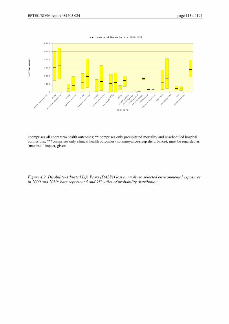
EFTEC/RIVM report 481505 024 page 113 of 194
∗comprises all short term health outcomes; ** comprises only precipitated mortality and unscheduled hospitaladmissions; ***comprises only clinical health outcomes (no annoyance/sleep disturbance), must be regarded as‘maximal’ impact, given
Figure 4.2. Disability-Adjusted Life Years (DALYs) lost annually to selected environmental exposuresin 2000 and 2030; bars represent 5 and 95%-tiles of probability distribution.
e n v ir o n m e n t a l d i s e a s e b u r d e n 2 0 0 0 - 2 0 3 0
0
1 0 0 0
2 0 0 0
3 0 0 0
4 0 0 0
5 0 0 0
6 0 0 0
partic
ulate a
ir poll
ution
* 200
0
2030
EC
partic
ulate
air po
llutio
n** 2
000
2030 E
C
tropo
spheri
c ozo
ne* 2
000
2030
EC
tropo
spheric
ozon
e** 2
000
2030
EC
noise r
oad t
raffic
*** 2
000
2030
EC
noise
air tr
affic*
** 20
00
2030
EC
UV 2000 n
o protoc
ol
UV 2000
Copen
hage
n
UV 2030 n
o prot
ocol
UV 2030
Copenha
gen
UV 2030
Mon
treal
indoor
radon
2000 (
1970
ref)
2020
(197
0 ref)
home d
ampn
ess 2
000
2020
food b
orne i
nfect.
2000
e x p o s u r e
DA
LY
s los
t ann
ually

page 114 of 194 EFTEC/RIVM report 481505 024

EFTEC/RIVM report 481505 024 page 115 of 194
5. Public opinion in the NetherlandsThe number of Dutch people that consider environmental protection and the fight against pollution asan ‘urgent and immediate problem’ has fluctuated slightly throughout the last decade. Although theenvironment was seen as less of a problem in 1999 than in 1995, when the concern was at its highest(63% in 1986, 80% in 1995 and 70% in 1999) (Eurobarometer, 1986, 1995), it remains a commonconcern for the Dutch.
5.1 Environmental issues in generalWhen considering environmental issues, there is a distinction between threats to the environment,threats to family health, local problems and national / international issues. All issues cited in thissummary are seen as being more threatening to the environment rather than health.
Drawing upon all the survey results, the issues considered to constitute a ‘serious threat to theenvironment’ (regardless of locality) are listed in Table 5.1.
Table 5.1 Issues considered to constitute serious environmental damageIssue Ranking
Factories releasing dangerous chemicals into the air or water 1Oil pollution of the seas and coasts 2Global pollution (gradual disappearance of tropical forests, destruction ofthe ozone layer, greenhouse effect etc)
3
Storage of nuclear waste 4Industrial Waste 5Acid Rain 6Excessive use of herbicides, insecticides and fertilisers in agriculture 7Rubbish in the streets, in green spaces or on beaches 8Air pollution from cars 9Uncontrolled mass tourism 10Sewage 11Noise generated by building or public works, heavy traffic, airports 12Source: Eurobarometer: Europeans and their Environment, 1992, 1995 and SCP survey 1993.
These opinions are fairly resilient to time and results from 1992 show similar rankings, (excepting theissue of acid rain, which has increased in importance slightly since 1992).
5.2 Global environmental issuesGlobal concerns are still high on the public agenda as listed in Table 5.2 and there is no sign of‘environmental fatigue’. When asked about global threats to the environment, the destruction oftropical forests was seen as ‘very worrying’ and as the most immediate threat. This was followed bythe disappearance of biodiversity and threats to natural habitats and the risk that pollution from theindustrialised countries spreads to less industrialised countries. The public are also ‘stronglyconcerned’ about the depletion of natural resources.
Seen as less of a threat, but, still ‘worrying’ to the public are the issues of global warming, (which wasseen as a threat to both environment and personal health), acid rain and the depletion of the ozonelayer. Despite the coverage of these issues in the media over the last decade, there is little evidence ofpublic ‘fatigue’.

page 116 of 194 EFTEC/RIVM report 481505 024
Table 5.2 International environmentalconcerns
Issue Average score(4-very worried,
1 – not at all worried)
Ranking
Disappearance of tropical forests 3.6 1Disappearance of certain types of plants, animalsand habitats throughout the world
3.3 2
Risk that pollution from the industrialised countriesspreads to less industrialised countries
3.3 2
Depletion of natural resources throughout the world 3.2 3Global warming (greenhouse effect) 3.1 4Destruction of the ozone layer 3.1 4Acid Rain 3.1 4Source: Eurobarometer, 1992 and 1995.
5.3 National environmental issuesThere is a slight difference in this prioritisation when considering threats within ‘one’s own country’.In this case, the results are listed below in Table 5.3.
Table 5.3 Concerns when considering one’s own countryIssue Average Score
4-very worried,1-not veryworried
Ranking
Industrial waste 3.1 1Pollution of seas and coasts 3.0 2Harm caused to animals, plants and the natural habitat 3.0 2Risks connected with the use of nuclear power 3.0 2Air pollution 2.9 3Pollution of rivers and lakes 2.9 3Pollution of agricultural origin (insecticides, slurryetc)
2.8 4
Urban sprawl 2.8 4Possible risks for the environment from thedevelopment of new bio-technologies
2.7 5
Motor sports in the countryside like outboard, motor-cross, trials, off road, jet skis or snow skis
2.7 5
Risks connected with industrial activities 2.7 5Natural disasters like floods, landslides, earthquakes,fires
2.5 6
Growth caused by tourism 2.5 6Hunting 2.2 7Source: Eurobarometer: Europeans and their Environment, 1992, 1995 and SCP survey 1993.
All the issues listed in Table 5.3 provoke concern, with the scale between ‘slightly worried’ forhunting to ‘worried’ for issues such as industrial waste. The aspects of the environment provokingmost concern are industrial waste, biodiversity loss and harm to animals, plants and the naturalhabitat, pollution of seas and coasts and pollution of rivers and lakes.

EFTEC/RIVM report 481505 024 page 117 of 194
5.4 Attitudes towards the futureThat environment is seen as an important issue does not stop the public being fairly confident aboutthe future and the level of concern about environmental disaster is low among the public as is thelevel of comprehension of risk, as shown in Table 5.4. However, there is no sign of ‘environmentalfatigue’ and support for more information campaigns on how to support the environment is very highas is the willingness to sacrifice personal activities for the sake of a better environment.
Table 5.4 Attitudes toward the futureIssue 1=high, 6=low Level of concern
Support for info campaigns 1 highCollective action 1 highSupport for pricing instruments 3 MiddleConscious purchasing 4 Fairly lowComprehension of risk from cars 6 lowComprehension of risk 6 lowConcern for the future 6 lowSource: ISSP 1993 and Compass 1993.
When asked where the public obtain their environmental information, opinion shows a healthy trust inenvironmental institutions but this trust has been slightly shifted between 1992-1995 fromenvironmental institutions to scientists (SCP survey, 1997).
5.5 Environmental protection action- who is responsible?Government policy is still seen as a necessary condition for the solution of diverse environmentalproblems, and influencing politicians and government policy is still the key aspect of the activities ofsocial organisations. Also indicated is that environmental organisations are in a transition period intheir relationship with the Government. But, still, the Government is seen as having primaryresponsibility – that there are a great many environmental issues which are too large for theenvironmental organisations and their networks to handle. When the question of ‘how to improve theenvironment’ is addressed, the public are reasonably supportive of the polluter pays principle.However, in Holland, there is a preference for coercive measures and information campaigns and avery strong wish to have common environmental laws throughout Europe.
As far as public attitude and actions towards the environment go, although air pollution is regarded aspossibly the most important threat, the public are reluctant to cite private cars as a major source of thispollution. Threats to the environment are seen to be more a result of bad industrial activity thanpersonal activity, and although the majority of Dutch public support the introduction of green taxes,they are lagging in their personal application of measures to improve the environment and are averageor well below the European average doing so.

page 118 of 194 EFTEC/RIVM report 481505 024

EFTEC/RIVM report 481505 024 page 119 of 194
6. Prioritisation of environmental issuesIn order to determine a final ranking for the environmental issues in the Netherlands in order ofimportance we draw upon the results of the damage assessment (see Chapter 4), the public opinion inthe Netherlands (see Chapter 5) and the DALY assessment (see Section 4.8.2). Table 6.1 bringstogether the results of the three methods.
The final ranking for the environmental issues given in the end column of Table 6.1 is based on asimple ‘Borda count’, i.e. for each environmental problem sum the weighted ranking from the publicopinion, the damage assessment and the DALY procedure and divide by the number of totalenvironmental issues considered. It is necessary to weight the rankings in order to allow for thedifferent numbers of environmental issues considered in the different approaches, i.e. twelve issuesare considered in the public opinion survey, seven in the damage assessment and seven in the DALYapproach. For example, for climate change the ‘Borda count’ is found by the following calculation(5*7 + 3*12 = 71)/19. The overall ranking is found by ordering the results of the ‘Borda count’, wherelower values score higher priorities. Although the ‘Borda count’ is a conventional way to rank anumber of rankings, the main disadvantage of this procedure is that the overall rankings are notsensitive to the uncertainty associated with the damage assessment for each environmental problem.To qualify the final rankings, Table 6.1 includes an assessment of overall uncertainty for eachproblem in the final column, using a scale of ‘++ to –-‘, where ++ indicates low uncertainty and --indicates high uncertainty.
Table 6.1 Environmental issues in the Netherlands in order of priorityEnvironmental
problemRanking
according todamage
assessment
Rankingaccording to
publicopinion
rankingaccording
toDALYs
‘Bordacount’
finalranking
uncertainty
Land contamination 2 - - 14/7 1 --Climate change 5 3 - 71/19 2 ++PM10 3 9 1 136/26 3 +Acidification 4 6 - 100/19 4 ++Low level ozone 1 9 4 143/26 5 +Eutrophication 7 7 - 133/19 6 --Noise 6 12 3 207/26 7 -No of issuesconsidered insurvey
7 12 7
Note that, public opinion rankings are taken from the results of the Eurobarometer (1992, 1995).These surveys ask the Dutch public their opinion about environmental issues, regardless of locality,and most of the environmental issues analysed in this study are included. However, it is necessary tomake some assumptions, firstly, we assume that ‘excessive use of herbicides, insecticides andfertilisers in agriculture’ corresponds to ‘eutrophication’ as defined in this study, although weacknowledge this is an imprecise correspondence as there are other impacts of ‘excessive’ use of thesechemicals, whilst ‘air pollution from cars’ is assumed to represent both PM10 and low level ozone.Unfortunately land contamination was not included in the public opinion surveys. The rankings forpublic opinion will not necessarily be the same as the damage assessment results. There should besome links because if people say they care then generally this means they are willing to pay to preventenvironmental damage.
Although the damage assessment is considered very uncertain for land contamination, we include it inthe overall ranking of environmental issue in order to determine whether the Netherlands is right tocommit so much expenditure to this issue.

page 120 of 194 EFTEC/RIVM report 481505 024
From Table 6.1 we can conclude that:
• land contamination scores 2nd priority from the damage assessment, whilst the overall rankingmethod places it at top priority. As Table 6.1 indicates the damage assessment is considered to bevery uncertain;
• climate change is ranked 3rd out of twelve problems considered by the public opinion survey, ifwe rank the public opinion results according to the seven issues considered in this study, climatechange would be the top priority. The damage assessment procedure gives climate change a highranking at 5th place. The overall ‘Borda count’ ranking suggests climate change is one of the toppriority issues for the Netherlands at 2nd place;
• PM10 is ranked 3rd by the damage assessment and 3rd by the Dutch public when ranked accordingto the seven issues of this study only and 1st by the DALY approach. Overall particulate matter isone of the top three environmental issues;
• the Dutch public rank acidification 6th out of twelve problems or 2nd priority when rankedaccording to the seven issues of this study only, whilst the damage assessment methodology givesacidification a priority at 4th. The overall ranking, based on the 'Borda count' suggestsacidification is 4th;
• low level ozone is ranked 9th out of twelve problems by Dutch public opinion, which correspondsto 3rd, if we rank according to the seven issues of this study only. The damage assessment resultsrank this environmental problem as a top priority and the DALY methodology suggests low levelozone ranks 4th out of seven issues. Overall the ‘Borda count’ result suggests low level ozone isnot a priority issue for the Netherlands and places low level ozone at 5th;
• eutrophication is given a low priority by both the Dutch public (7 out of twelve problems, or 5th
out of seven problems) and the damage assessment procedure at 7th. This is reflected in theoverall ranking place of second least priority. Note, however that the damage estimates foreutrophication are acknowledged as extremely uncertain;
• noise is ranked as the lowest priority problem by the Dutch public. The damage assessmentmethodology also ranks noise low at 6th, whilst the DALY approach ranks noise as 3rd highestpriority out of seven issues. The final ranking suggests noise nuisance is least priority issue forthe Netherlands.

EFTEC/RIVM report 481505 024 page 121 of 194
Definitions2xCO2: the scientific research on global warming impacts has almost entirely focused onthe case of CO2 concentration doubling, i.e. the impacts of an atmospheric CO2concentration of twice the preindustrial level (2 x CO2). This a completely arbitrarybenchmark, chosen soley for analytical convenience. It is neither an optimal point nor asteady state and warming will continue and may in fact worsen beyond 2 x CO2.
Annuitisation factors: sometimes it is more useful to represent damage estimates (given aspresent values using an agreed discount factor) as an annual sum, i.e. an annuity. Anannuity is simply an annual sum, which when discounted at the relevant discount rate,would give the present value in question. We use the following formula to establish therelevant annuity, A:A = PV. (s/(1+s))Where A = annuity, PV = present value, s= discount rate
Contingent valuation methodology: estimates the WTP for a change in the quantityand/or quality of an environmental good by using survey techniques (Mitchell and Carson,1989). WTP is estimated by way of implementing a structured questionnaire to arepresentative sample of the population of concern. In the questionnaire a hypotheticalchange is described and the respondent is asked directly for her WTP for this change. Thevaluation questions are supplemented by questions on socio-economic characteristics andrelevant attitudes and preferences regarding the good in question. This information is usedto estimate a valuation function which 'explains' WTP as a function of these variables. Inorder to obtain a valid response it is crucial to provide an accurate and meaningfuldescription of: (i) the change that is valued, (ii) the way and how often the respondent isexpected to pay and also respondents must be reminded of their budget constraints. Forfurther details see Freeman (1993).
Cost - benefit analysis: procedure for estimating gains (benefits) and losses (costs) of aproject or policy in monetary terms and comparing these estimates.
Discount rate: the rate at which future costs and benefits are adjusted downwards toreflect, for example, that current benefits or costs are valued more highly than future costsor benefits.
Hedonic price technique: the underlying concept of the hedonic price technique is that theprice of a good, for example, a house, is a function of its attributes, such as the number ofrooms, size, location, and environmental characteristics, such as noise levels and ambientair quality and others. The HPT proceeds by estimating an hedonic price function byregressing house price on the relevant characteristics. In the simplest form of the method, ameasure of the value of an environmental characteristic of interest, such as noise, can bededuced by differentiating the hedonic price function with respect to noise. For furtherdetails refer to Freeman (1993).
Purchasing Power Parity (PPP) is defined as the rates of currency conversion thatequalises the purchasing power of different currencies by eliminating the differences inprice levels between countries. They are relative prices. For example, if the price ofcauliflower in France is 8.00 francs and in the United State it is 1.50 dollars, then the PPPfor cauliflower between France and the US is 8.00francs to 1.50 dollars or 5.33francs to thedollar. This means that for every dollar spent on cauliflower in the United States, 5.33francs would have to be spent in France to obtain the same quantity and quality or, in otherwords, the same volume of cauliflower, www.oecd.org/std/ppp/pppbackground.
page 122 of 194 EFTEC/RIVM report 481505 024
Present value: is the value of future amounts in current terms the following formula is usedto establish present value damage estimates over the period infinity:
PV = X . (1+s) / (s-g)Where PV = present value, X = undiscounted damages in 1995, s = discount rate (i.e. 6%)and g is the growth rate of damages over time, i.e. between 1995 and 2030.
Primary benefits: avoided environmental damage from issue A due to environmentalcontrol policies targeted at issue A.
Secondary benefits: avoided environmental damage from issue B due to environmentalcontrol policies targeted at issue A.
Total benefits: the sum of primary benefits and secondary benefits.
Uncertainty: deficiency in knowledge about events with an unknown probability ofoccurrence.
Value of a Statistical Life: the sum of individuals' own valuations of risks to their ownlives (refer to Annex A3).

EFTEC/RIVM report 481505 024 page 123 of 194
References
Abbey, D.E., Lebowitz, M.D., Mills, P.K., Petersen, F.F., Lawrence Beeson, W. and Burchette, R.J.(1995) ‘Long-terms Ambient Concnetrations of Particulates and Oxodants and Development ofChronic Disease in a Cohort of Non-smoking California Residents’, Inhalaltion Toxicology, 7: 19-34.
AEA Technology (with Eyre Energy Environment and Metroeconomica) (1998a) Cost BenefitAnalysis of Proposals under the UN ECE Multi-Pollutant, Multi-Effect Protocol, final report for theDepartment of the Environment, Transport and the Regions, London.
AEA Technology (1999) Economic Appraisal of Porposals Under the UNECE Multi-Effects andMulti-Pollutant Protocol, report commissioned by EC DGXI for UNECE/TFEAAS.
Alfsen, K., Birkelund, H. and Aaserud, M., (1995). Impacts of an EC Carbon/Energy andDeregulating Thermal Power Supply on CO2, SO2 and NOx Emissions, Environment and ResourceEconomics, 5, 165-189
Alfsen, K., Brendemoan, A. and Glomsrod, S., (1992). Benefits of Climate Policies: Some TentativeCalculations, Discussion Paper 69, Central Bureau of Statistics, Oslo.
Anderson, H.R., Ponce de Leon, A., Bland, J.M., Bower, J.S. and Strachan, D.P. (1996) ‘Air Pollutionand Daily Mortality in London: 1987-92. British Medical Journal 312: 665-69.
Ayres, R and Walter, J., (1991), The greenhouse effect: damages, costs and abatement, Environmentaland Resource Economics, 1, 3, 237-70
Azar, C. and Sterner, T., (1996), Discounting and distributional considerations in the context of globalwarming, Ecological Economics, 19, 169-184
Azar, C., (1999), Weight factors in cost-benefit analysis of climate change, Environmental andResource Economics, 13, 249-268
Barker, T., (1993). Secondary Benefits of Greenhouse Gas Abatement - The Effects of a UKCarbon/Energy Tax on Air Pollution, Department of Applied Economics, Cambridge University,Mimeo.
Bateman, I., Day, B., Lake, I. and Lovett, A., (1999). The Effect of Road Traffic on Residential PropertyValues: a Literature Review and Hedonic Pricing Study, Report to the Scottish Office, Edinburgh.
Becker. J.W., Broek. A.vd., Dekker, P. and Nas, M., (1996). Pubileke opinie en mileu, (Eenverkenning van het sociale draagvlak voor het milieubelieid op grond van survey-gegevens),
Benefits of Reduced Air Pollution in the US from Moderate Greenhouse Gas Mitigation Policies inthe Electricity Sector, Resources for the Future Discussion Paper 99-51, Resources for the Future,Washington DC.
Bertrand, N., (1997). Meta-Analysis of Studies into Willingness to Pay to Reduce Traffic Noise,CSERGE, University College London, London.
Bleijenberg, A., Berg, W. van der, and Wit, G. de, (1994). The Social Costs of Traffic: a LiteratureReview, Centrum voor Energiebesparing en Schone Technologie, Delft.
Bockstael, N.E., K.E. McConnell and I.E. Strand (1989) ‘Measuring the Benefits of Improvements inWater Quality: The Chesapeake Bay’, Marine Resource Economics, 6(1): 1-18.

page 124 of 194 EFTEC/RIVM report 481505 024
Bockstael, N.E., W.M. Hannemann and C.L. Kling (1987) ‘Estimating the Value of Water QualityImprovements in a Recreational Demand Framework’, Water Resources Research, 23(5): 951-960.
Bonenschansker, E., Leijsen, M. and Groot, H de., (1995). The Price of Mobility in the Netherlands,Institte for Research on Public Expenditure, The Hague.
Boyd,R., Krutilla, K. and Viscusi, W.K., (1995). Energy taxation as a policy instrument to reduce CO2emissions: a net benefit analysis, Journal of Environmental Economics and Management, 29, 1-24.
Boyl, K.J. and Bergstrom, J.C. (1992). Benefit Transfer Studies: Myths, Pragmatism and Idealism,Water Resources Research, 28, 3, pp 657-663.
Bruce, J.P., Lee, H. and Haites, E.F., (1996) Climate Change 1995: Economic and Social Dimensionsof Climate Change, Cambridge University Press, Cambridge, UK.
Burtraw, D and Toman, M., (1997), The Benefits of Reduced Air Pollutants in the US fromGreenhouse Gas Mitigation Policies, Resources for the Future Discussion Paper 98-01, Resources forthe Future, Washington DC.
Burtraw, D., Krupnick, A., Palmer, K., Paul, A., Toman, M. and Bloyd, C., (1999), Ancillary
CEC (1995 and 1997). ExternE: Externalities of Energy, Office for Official Publications of the EuropeanCommunities, Luxembourg.
Choe, K., Whittington, D. and Lauria, D. (1994) ‘The Economic Benefits for Surface Water QualityImprovements in Developing Countries: A Case Study of Davao, Philippines’, Land Economics72(4): 519-537.
Christensen, P., Beaumont, H., Dunkerley, C., Lindberg, G., Otterstrom, T., Gynther, L., Rothengatter,W. and Doll, C., (1998), Pricing European Transport Systems: D7 Internalisation of externalities,Appendix, Institute for Transport Studies, University of Leeds.
Cline, W., (1993). The Economics of Climate Change, Institute for International Economics,Washington DC.
Collins, A. and Evans, A., (1994). Aircraft noise and residential property values: an artificial neuralnetwork approach, Journal of Transport Economics and Policy, May, 175-197.
CSERGE (Centre for Social and Economic Research on the Global Environment, University CollegeLondon and University of East Anglia, Deprtment of Economics and Social Sciences at the AgriculturalUniversity of Norway, Institute for Envionmental Studies at the Amsterdam Free University, Centre forApplied Studies at the Catholic University of Portugal and the Department of Applied Economics at theUniversity of Vigo, (1999). Benefits Transfer and the Economic valuation of Environmental Damage inthe European Union: with Special Reference to Health, European Union's Environment and ClimateResearch Programme (1994-1998): Theme 4 Human dimensions of Environmental Change.
Dab, W., Quenel, S.M.P, Le Moullec, Y., Le Tertre, A., Thelot, B., Monteil, C., Lameloise, P., Pirard,P., Momas, I., Ferry, R., and Festy, B. (1996) ‘Short-term Respiratory Health Effects of Ambient AirPollution: Results from the APHEA Project in Paris’, Journal of Epidemiology and CommunityHealth 50 (suppl 1): S42-46.
Dockrey, D.W., Speizer, F.E., Stram, D.O., Ware, J.H., Spengler, J.D. and Ferries, B.G. (1989)‘Effects of Inhalable Particles on Respiratory Health of Children’, American Review of RespiratoryDisease, 139: 587-594.

EFTEC/RIVM report 481505 024 page 125 of 194
Dowlatabadi, H., Schang, T. and Siegel, S., (1993). Estimating the Ancillary Benefits of SelectedCarbon Dioxide Mitigation Strategies: Electricity Sector, Climate Change Division, US EPA,Washington DC.
Dusseldorp, A., Kruize, H., Brunekreef, B., Hofschreuder, P., de Meer, G., and van Oudcorst, A.B.(1995) Associations of PM10 and Airborne Iron with Respiratory Health of Adults Near a SteelFactory, American Journal of Respiratory Critical Care Medicine, 152: 1932-39.
Economic Research and Advisory Consortium (ERECO) (1992). Overview and Estimation of CurrentEnvironmental Expenditure in the EC, for the European Commission, Directorate General XI,Brussels.
Ekins, P., (1996). How Large A Carbon Tax is Justified by the Secondary Benefits of CO2Abatement? Resource and Energy Economics, 18, 161-187.
Eurobarometer 43.1 bis, (1995). Europeans and their Environment, European Commission, Brussels.
Eurobarometer 46, (1996). Public Opinion in the European Union: The Importance of EnvironmentalIssues, European Commission, Brussels.
Eurobarometer 51, (1999). Public Opinion in the European Union, p 91. European Commission,Directorate General X, Brussels.
European Conference of Ministers of Transport (ECMT) (1998), Efficient Transport for Europe: Policiesfor the Internalisation of External Costs, ECMT/OECD, Paris.
Eurostat, (1995). Europe in Figures, Fourth edition, Brussels.
ExternE, (1997), ExternE National Implementation the Netherlands: Externalities of electricityproduction in the Netherlands, Dorland, C. Jansen, H.M.A., Tol, D. and Dodd, D. of the Institute forEnvironmental Studies (IVM), Vrije Univresitiet, Amsterdam research for the European Commission,JOULE III.
ExternE (1998), Externalities of Energy: Methodology Annexes, European Commission DGXII.
Eyre, N., Downing, T., Hoekstra, R., Rennings, K. and Tol, R., (1997). Global Warming Damages,Final Report of the ExternE Global Warming Sub-Task, DGXII, European Commission, Brussels.
Fankhauser, S. (1995). Valuing Climate Change: the Economics of the Greenhouse, Earthscan,London.
Fankhauser, S., Tol, R. and Pearce, D.W. (1997a). Extensions and Alternatives to Climate ChangeImpact Valuation: on the Critique of IPCC Working Group III's Impact Estimates, Environment andDevelopment Economics, forthcoming.
Fankhauser, S., Tol, R. and Pearce, D.W. (1997b). The Aggregation of Climate Change Damages: aWelfare Theoretic Approach, Environment and Resource Economics, Vol.10, No.3, October, 249-266.
FAO Statistical Database, (2000). http://apps.fao.org.
Feenberg, D. and Mills, E.S. (1980) Measuring the Benefits of Water Pollution Abatement, AcademicPress.
Feitelson, E., Hurd, R. and Mudge, R., (1995). The impact of airport noise on willingness to pay forresidences, Transportation Research.

page 126 of 194 EFTEC/RIVM report 481505 024
Flores, N. and Carson, R. (1997), The Relationship Between the Income Elasticities of Demand andWillingness to Pay, Journal of Environmental Economics and Management, 33, 287-295
Freeman, A.M., (1993). Measurement of Environmental Resource Values: Theory and Methods,Resources for the Future, Washington, DC.
Georgiou, S., Langford, I., Bateman. I., Turner. R.K. 1996. ‘Determinants of individuals’ WTP forreductions in environmental health risks: a case study of bathing water quality’. CSERGE WorkingPaper 96-14, UEA.
Georgiou, S., Langford, I., Bateman. I., Turner. R.K. (1998) ‘Determinants of individuals’ WTP forreductions in environmental health risks: a case study of bathing water quality’ Environment andPlanning, 30: 577-594.
Glomsrod, S. (1990), Stabilization of Emissions of CO2: a Computable General EquilibriumAssessment, Discussion Paper No.48, Central Bureau of Statistics, Oslo.
Goulder, L. (1993). Environmental taxation and the double dividend: a reader’s guide, InternationalTax and Public Finance, 2, 157-183.
Green, C.H. and Tunstall, S.M. (1991) The evaluation of river water quality improvements by thecontingent valuation method. Applied Economics, 23, 1135-1146
Green, C.H. and Willis, K.G. (1996) New non-use and angling economic data. Report to Foundationfor Water Research, Marlow, Bucks.
Grue, B., Langeland, J. and Larsen, O., (1997). Housing Prices: Impacts of Exposure to Road Traffic andLocation, TOI Report, 351, Oslo.
Halomo, J., (1992). The impact of road traffic on unbuilt real estate values (in Finnish), FinnishTechnological research Institution, Espoo.
Hanley, N. (1989) Problems in valuing environmental improvements resulting from agriculturalpolicy changes: the case of nitrate pollution. In Economic aspects of environmental regulations inagriculture (ed. A. Dubgaard and A. Nielsen), Wissenschatfsverlag Vauk Kiel, Kiel.
Hoek, G.; Verhoeff, A.; Fischer, P. (1997). Daily mortality and air pollution in the Netherlands, 1986-1994. Report nr. 1997-481. Environmental and Occupational Health Group, Wageningen
Hollander, A.E.M. de., Melse J.M., Lebret. E., Kramers P.G.N. An aggregate public health indicator torepresent the impact of multiple environmental exposures. Epidemiol 1999: 10: 606-17.
IISP, The Data Archive, University of Essex, ‘Environment’, 1993. The Economic and SocialResearch Council and the Joint Information Systems Committee
Intergovernmental Panel on Climate Change (IPCC), (1995). Working group III: Second AssessmentReport, Cambridge University Press, Cambridge.
Iten and Maggi, 1995, cited in Pearce (1995), op cit.
Johannesson, M., and Johansson, P-O. (1996) To Be or Not to Be, That Is the Question: An EmpiricalStudy of the WTP for an Increased Life Expectancy at an Advanced Age, Journal of Risk andUncertainty, 13, pp 163-174.
Johansson, O., (1996). The external costs of road transport in Sweden, in D. Maddison et al., 1996.Blueprint 5: The True Costs of Road Transport, Earthscan, London,153-177.

EFTEC/RIVM report 481505 024 page 127 of 194
Jones, H., Howson, G., Rosengren-Brink, U., Hornung, M., and Linareas, P. (1997) Review of theEffects Of air Pollutants on Agricultural Crops, Forestry and natural Vegetation, Institute onTerrestrial Ecology, Report T707074f5, ITE, Merlewood, UK.
Kristrom, B. and Riera, P. (1996) Is the Income Elasticity of Environmental Improvements Less ThanOne? Environmental and Resource Economics, 7, 45-55.
Krupnick, A.J., Harrington, W., and Ostro, B. (1990) Ambient Ozone and Acute Health Effects:Evidence from Daily Data, Journal of Environmental Economics and Management, 18, pp 1-18.
Kucera, V. (1994) The UNECE International Cooperative Programme on Effects on Materials,including Historic and Cultural Monuments, report to the working group on effects within the UNECE in Geneva, Swedish Corrosion Institute, Stockholm, Sweden.
Lant, C.L. and Roberts, R.S. (1990) Green belts in the cornbelt: riparian wetlands, intrinsic values andmarket failure. Environment and Planning, 22, No. 10, 1375-88
Lee, D.S., Holland, M.R., Falla, N. (1995), The potential impact of ozone on materials in the UK,Atmospheric Environment, vol 30, p. 1053-1065.
Lutter, R. Shogren, J. (1999), Reductions in local air pollution restrict the gain from global carbonemissions trading, American Enterprise Institute, Washington DC and Department of Economics,Wyoming University, mimeo.
Machado, F. and Mourato, S. (1998) ‘Improving the Assessment of Water Realted Health Impacts:Evidence from Coastal Waters in Portugal’, Paper presented at the first World Congress onEnvironmental and resource Economics, Venice, June 25-27, 1998.
Maddison, D. (1994). The Shadow Price of Greenhouse Gases and Aerosols, CSERGE, UniversityCollege London, mimeo.
Maddison D., Pearce. D.W., Johansson, O., Calthrop. E., Litman, T. and Verhoef, E., (1996). Blueprint 5:The True Costs of Road Transport, Earthscan, London.
Maddison, D., Pearce, D.W., and Lvovsky, K. (1997). Damage Costs from Fuel Use in Major UrbanConurbations, Environment Department, World Bank, Washington DC (restricted).
Maddison, D. (1998). Valuing Changes in Life Expectancy in England and Wales Caused by AmbientConcentrations of Particulate Matter, CSERGE, University College London, UK, mimeo.
McConnell, K. and Ducci, J. (1989) Valuing Environmental Quality in Developing Countries: TwoCase Studies’ Paper presented to Applied Social Science Association, Atlanta, Georgia.
Melse et al., AJPH 2000.
Mendelsohn, R., Morrison, R.W., Schlesinger, M. Andronova, N. (1996). Global Impact Model forClimate Change, Unpublished mss, School of Forestry, Yale University.
Mendelsohn, R. and Neumann, J. (eds), (1999). The Impact of Climate Change on the US Economy,Cambridge University Press, Cambridge.
Middlesex University (1994) The evaluation of the recreational and other use values from alleviatinglow flows. NRA, R&D Note 258.

page 128 of 194 EFTEC/RIVM report 481505 024
MSC-W Meteorological Synthesizing Centre - West of EMEP (1995). European TransboundaryAcidifying Air Pollution: ten years calculated fields and budgets to the end of the first SulphurProtocol, MSC-W, EMEP, Oslo.
Murray, C.J.L., Lopez, A.D. (eds), (1996). The global burden of disease; a comprehensive assessmentof mortality and disability from disease, injury, and risk factors in 1990 and projected to 2020. Globalburden of disease and injury series, volume I, Harvard University Press.
Nas, M., Dekker, P. and Hemmers, C. (1997). Maatschappelijke organisaties, publieke opinie enmileu, Sociaal en Cultureel Planbureau, Rijswijk.
NERA and CASPAR, (1997). Valuation of Deaths from Air Pollution, Report to the Department of theEnvironment, Transport and Regions.
Nordhaus, W. (1991). To slow or not to slow: the economics of the greenhouse effect. EconomicJournal, 101, 407, 920-937.
Nordhaus, W. (1994). Managing the Global Commons: the Economics of Climate Change, MITPress, Cambridge, Mass.
Nordhaus, W. (1998). Roll the DICE Again: the Economics of Global Warming, unpublished mss.
Odegaard, H. (1996) Environmental Impact and Cost Efficiency in Municipal Wastewater Treatment,University of Trondheim, Norway.
OECD (1993), Environmental Data Compendium, OECD, Paris.
OECD (1999), Ancillary Benefits of Climate Change Policies, ENV/EPOC/GEEI(99)16, EnvironmentDirectorate, OECD, Paris.
Ostro, B.D. (1987) ‘Air Pollution and Mortality Revisited: A Specification Test’, Journal ofEnvironmental Economics and Management, 14: 87-98.
Ostro, B.D. and Rothschild, S. (1989) Air Pollution and Acute Respiratory Morbidity: AnObservational Study of Multiple Pollutants, Environmental Resources, 50: 238-47.
Pearce, D.W. (1980), The Social Incidence of Environmental Costs and Benefits, in T.O'Riordan andR.K.Turner (eds), Progress in Resource management and Environmental Planning, Vol.2, John Wileyand Son, London.
Pearce, D.W. (1992), The secondary benefits of greenhouse gas control, CSERGE Working Paper 92-12, CSERGE, University College London.
Pearce, D.W., Cline, W.R., Achanta, A., Fankhauser, S., Pachauri, R., Tol, R. and Vellinga, P. (1996).The Social Costs of Climate Change: Greenhouse Damage and the Benefits of Control, inIntergovernmental Panel on Climate Change, Climate Change 1995: Economic and SocialDimensions of Climate Change, Cambridge University Press, Cambridge, 183-224.
Pearce. D.W. 1998. Valuing Statistical Lives: Briefing Paper for: Economic Assessment of Priorities fora European Environmental Policy Plan, CSERGE, University College London and EFTEC, London.
Pearson, M. (1992) Recreational and environmental valuation of Rutland Water. Chapter 5 ofUnpublished PhD thesis, University of East Anglia, Norwich.
Peck, S. and Teisberg, T. (1993). Global warming uncertainties and the value of information: ananalysis using CETA, Resource and Energy Economics, 15, 1, 71-97.

EFTEC/RIVM report 481505 024 page 129 of 194
Pennington, G., Topham, N. and Ward, R., (1990). Aircraft noise and residential property values adjacentto Manchester International Airport, Journal of Transport Economics, 24, 1, 49-59.
Pommerehne, K., (1988). Measuring Environmental Benefits: Comparison of a Hedonic technique andCVM, in D.Bos, M.Rose and C.Seidl, (eds), Welfare and Efficiency in Public Economics, Berlin.
Ponce de Leon, A., Anderson, H.R., Bland, J.M., Strachan, D.P., and Bower, J. (1996) Effects of AirPollution on Daily Hospital Admissions for Respiratory Disease in London Between 1987-1988 and1991-1992, Journal of Epidemiology & Community Health, 50 (Supplement 1), S63-S71.
Pope, C.A. and Dockery, D.W. (1992) Acute Health Efects of PM10 Pollution on Symptomatic andAsymptomatic Children, American Review of Respiratory Disease, 145: 1123-1126.
Pope, C.A. III, Thun, M..J., Namboodiri, M.M., Dockery, D.W., Evans, J.S., Speizer, F.E. and Heath,C.W. Jr. (1995). ‘Particulate Air Pollution as Predictor of Mortality in a Prospective Study of USAdults’, American Journal of Respiratory Critical Care Medicine, 151: 669-674.
Rabl A. and Eyre. N. (1997) An Estimate of Regional and Global O3 Damage from Precursor NOx andVOC Emissions, Ecole des Mines, Paris and Eyre Energy and Environment, Carnforth.
Ready, R., Navrud, S., Day, B., Dubourg, R., Machado, F., Mourato, S., Spanninks, F., andRodriquez, M.X.V. (1999), Benefit Transfer in Europe: Are Values Consistent Across Countries?Paper presented at seminar January 20th 2000, University College London.
RIVM, EFTEC, NTUA and IIASA, (2000), European Environmental Priorities: an Environmentaland Economic Assessment, Report to DGXI of the European Commission (under completion).
Roemer, W., Hoek, G. and Brunekreef, B. (1993) Effect of Ambient Winter Air Pollution onRespiratory Health of Children with Chronic Respiratory Symptoms, American Review of RespiratoryDisease, 147: 118-124.
Roughgarden, T. and Schneider, S. (1999), Climate change policy: quantifying uncertainties fordamages and optimal carbon taxes, Energy Policy, 27, 415-429.
Rowe, R., Lang, C., Chestnut, L., Latimer, D., Rae, D., Bernow, S. and White, D. (1995), The NewYork Electricity Externalities Study, Vols 1 and 2, Oceana Publications, New York.
Rowlatt, P., Spackman, M., Jones, S., Jones-Lee, M., and Loomes, G. (1998) Valuation of Deathsfrom Air Pollution, NERA and CASPAR, Report to UK Department of the Environment, Transportand Regions.
Søderqvist. T. (1995). The Benefits of Reduced Eutrophication of the Baltic Sea: a Contingent ValuationStudy, Stockholm School of Economics, Stockholm, mimeo.
Saelensminde, K. and Hammer, F., (1994). Assessing Environmental Benefits by Means of ConjointAnalysis, Institute of Transport Economics, Oslo.
Saelensminde, K., (1997). Contingent Valuation of Urban Traffic Air Pollution and Noise, Institute ofTransport Economics, Oslo.
Sandstrøm . M. (1994). A Discrete Choice Model of Swedish Beach Recreation, Stockholm School ofEconomics, Stockholm, Mimeo.
Scheraga, J. and Leary, N. (1993), Costs and side benefits of using energy taxes to mitigate globalclimate change, National Tax Journal, Proceedings, 133-8.

page 130 of 194 EFTEC/RIVM report 481505 024
Schipper, Y., (1998). Why do aircraft noise value estimates differ? A meta-analysis, Journal of AirTransport Management, 4 (1998) 117-124.
Schwartz, J. and Morris, R. (1995) Air Pollution and Hospital Admissions for Cardiovascular Diseasein Detroit, Michigan, American Journal of Epidemiology, 142: 23-35.
Soguel, N., (1994). Évaluation Monétaire des Atteintes à l'Environnement: une Étude Hedoniste etContingente sur l'Impact des Transports, University of Neuchâtel, Switzerland.
Strand, J., (1999). The relationship between property values and railroad proximity: a study based onhedonic prices and real estate brokers’ appraisals, Department of Economics, University of Oslo,mimeo.
Tinch, R., (1995). The Valuation of Externalities, Report to the UK Department of Transport, London.
Titus, J. (1992), The costs of climate change to the United States, in S.Majumdar (ed), Global ClimateChange: Implications, Challenges and Mitigation Measures, Pennsylvania Academy of Science,Easton, Pa.
Tol, R. (1995), The damage costs of climate change: towards more comprehensive estimates,Environmental and Resource Economics, 5, 353-374.
Tol, R. (1999), The marginal costs of greenhouse gas emissions, The Energy Journal, 20,1, 61-81.
Tol, R., Fankhauser, S. and Pearce, D.W. (1996). Equity and the Aggregation of the Damage Costs ofClimate Change in V.Nacicenovic, W Nordhaus, R Richels and F Toth (eds), Climate Change:Integrating Science, Economics and Policy, International Institute for Applied Systems Analysis,Laxenburg, Austria, 167-178.
Tol, R., Fankhauser, S. and Pearce, D.W. (1999). Empirical and ethical arguments in climate changeimpact valuation and aggregation, in F Toth (ed), Fair Weather? Equity Concerns in Climate Change,Earthscan, London, 65-79.
Tomkins, J., Topham, N., Twomey, J. and Ward, R., (1995). Noise, access and residential propertyvalues: the local externality effects of an airport, Journal of Transport Economics and Policy.
Tonneijck, A.E.G., van der Eerden, L.J., Wijnands, J.H.M., Bunte, F.H.J., Bremmer, J. and Hoogeveen,M.W, (1998). Economische aspecten van het effect van luchtverontreiniging op de gewasteelt inNederland. LEI-DLO, the Netherlands.
Turner. R. K. 1995. The Baltic Drainage Basin Report, EV5V-CT-92-0183, European Commission,Brussels.
Turner. R. K. 1997. Managing Nutrient Fluxes and Pollution in the Baltic: an InterdisciplinarySimulation Study, Centre for Social and Economic Research on the Global Environment, University ofEast Anglia and University College London, GEC Paper 97-17.
Vainio, M., (1995). Traffic Noise and Air Pollution: Valuation of Externalities with Hedonic Price andContingent Valuation Methods, Helsinki School of Economics and Business Administration, DoctoralDissertation.
Verhoef, E., (1996). The external costs of road transport in the Netherlands, in D. Maddison et al, 1996.Blueprint 5: The True Costs of Road Transport, Earthscan, London, 199-217.
Viscusi, W.K., Magat, W., Carlin, A. and Dreyfus, M. (1994), Environmentally responsible energypricing, The Energy Journal, 15, 2, 23-42.

EFTEC/RIVM report 481505 024 page 131 of 194
Vonk, J.M. and Schouten, J.P. (1998). Daily emergency hospital admissions and air pollution in theNetherlands, 1982-1986 and 1986-1995. Report nr. VROM reg #96.140072. Faculty of MedicalSciences, University of Groningen, Groningen, Netherlands.
Weinberger, M., Thomassen, H. and Willeke, R., (1991). Kosten des Lärms in der BundesrepublikDeutschland, Umweltbundesamt, Berichte 9/91, Berlin.
Whittemore, A.S., and Korn, E.L. (1980), Asthma and air pollution in the Los Angeles area,American Journal Public Health 70, 687 - 696.
Wordley, J., Walters, S. and Ayres, J.G. (1997) ‘Short-term Variations in Hospital Admissions andMortality and Particulate Air Pollution’ (In Press).
World Bank, (1993). World Development Report: Investing in Health – world development indicators.New York, Oxford University Press.
Yamaguchi, Y., (1996). Evaluating the cost of aircraft noise around airports in London, M.ScDissertation, University College London.
Zylicz. T., Bateman. I., Georgiou. S., Markowska. A., Dziegielewska. D., Turner. R. K., Graham A.,Langford . I. 1995a. Contingent Valuation of Eutrophication Damage in the Baltic Sea Region, CSERGEWorking Paper 95-03, CSERGE, University of East Anglia.

page 132 of 194 EFTEC/RIVM report 481505 024
EFTEC/RIVM report 481505 024 page 133 of 194
Annex I Methodology and assumptions
1. Monetary valuation techniquesIntroductionThe economic approach to valuing environmental changes is based on people’s preferences forchanges in the state of their environment. Environmental resources typically provide goods andservices for which there are either no apparent markets or very imperfect markets, but whichnevertheless can be important influences on people’s well-being. Examples include the quality of air,which affects people’s health, crop yields, damage to buildings, and acidification of forests and freshwaters.
However, the lack of markets for some of these services and existence of imperfect markets for othersmeans that unlike man-made products, they are not priced, therefore their monetary values to peoplecannot be readily observed. The underlying principle for economic valuation of environmentalresources, just as for man-made products, is that people’s willingness to pay (WTP) for anenvironmental benefit, or conversely, their willingness to accept compensation (WTA) forenvironmental degradation, is the appropriate basis for valuation.
If these quantities can be measured, then economic valuation allows environmental impacts to becompared on the same basis as financial costs and benefits of the different scenarios forenvironmental pollution control. This then permits an evaluation of the net social costs and benefitsof each scenario for each environmental issue.
The lack of markets and prices for many environmental goods and services means that the challengefor economists is twofold. The first task is to identify the ways in which an environmental changeaffects well-being. This is addressed in the next section, where the components of ‘total economicvalue’ of a resource are explained. The second task is to estimate the value of these changes througha variety of direct and indirect valuation techniques, exposition of which is given in the followingsections.
Total Economic ValueThe monetary measure of the change in society’s well-being due to a change in the quantity and / orquality of environmental assets or quality is called the total economic value (TEV) of the change. Toaccount for the fact that a given environmental resource provides a variety of services to society, TEVcan be disaggregated to consider the effects of changes on all aspects of well-being influenced by theexistence of the resource.
TEV can be divided into use values and non-use values, the latter also being called ‘passive usevalues’. Use values include:
• direct use values, where individuals make actual use of a resource for either commercialpurposes (e.g. harvesting timber from a forest) or recreation (e.g. swimming in a lake);
• indirect use values, where society benefits from ecosystem functions (e.g. watershed protectionor carbon sequestration by forests), and
• option values, where individuals are willing to pay for the option of using a resource in thefuture (for example, future visits to a wilderness area).
Non-use values can take the form of:
• existence values, which reflect the fact that people value resources for ‘moral’ reasons,unrelated to current or future use
• bequest values, which measure people’s willingness to pay to ensure their heirs will be able touse a resource in the future

page 134 of 194 EFTEC/RIVM report 481505 024
Typically it is not always easy or even necessary to separate existence and bequest values.
To arrive at an estimate of the net change in societal well-being arising from an environmentalchange, we must consider each of these elements in turn. The total economic value (TEV) of achange is the sum of both use and non-use values:
TEV = use values + non-use values
= direct use + indirect use + option + existence + bequest values
Table 1.1 presents a taxonomy for environmental resource valuation, using the total economic valueof a forest as an illustration.
Table 1.1 Economic taxonomy for environmental resource valuation
Total Economic Value
Use Values Non-use Values
Direct Use Indirect Use Option Value Bequest Value Existence Value
Outputs directlyconsumable
functionalbenefits
Future direct andindirect values
use and non-usevalue of
environmentallegacy
value fromknowledge of
continuedexistence
• food• biomass• recreation• health
• flood control• storm
protection• nutrient cycles
• biodiversity• conserved
habitats
• habitats• prevention of
irreversiblechange
• habitats• species• genetic• ecosystem
The first step in estimating any of these values is the definition and measurement of the environmentalimpact. This often includes an element of scientific uncertainty that can, at times, be quite significant.The accuracy of economic valuation is therefore dependent on accurate scientific identification andquantification of the environmental change in order to estimate people’s preferences for or against it.
Valuation TechniquesThe practical problem with economic valuation is one of deriving credible estimates of people’spreferences in contexts where there are either no apparent markets, or very imperfect markets. In thecase of marketed goods, the market price is the measure of willingness to pay and can be readilyobserved. However, in the case of non-marketed goods and services we need to elicit this value indifferent ways. There are two broad approaches to valuation, each comprising several differenttechniques, as illustrated in Figure 1.1.
• Revealed preference techniques, which infer preferences from actual, observed market-basedinformation. Preferences for environmental goods are revealed indirectly when individualspurchase marketed goods which are related to the environmental good in some way, and
• Stated preference techniques, which attempt to elicit preferences directly by use ofquestionnaire. All valuation of non-use values depends on these techniques.
We consider each of these approaches in turn, highlighting when each could be used, their advantagesand drawbacks .
Revealed Preference TechniquesThe essence of revealed preference techniques is that they infer environmental values from markets inwhich environmental factors have an influence. For example, there are markets for certain goods to

EFTEC/RIVM report 481505 024 page 135 of 194
which environmental commodities are related, as either substitutes or complements to the goods inquestion. In this way people’s actions in actual markets reflect, to a certain extent, their preferencesfor environmental assets.
There are four main revealed preference techniques that are considered in the sections that follow.
1. Averting behaviour
2. Hedonic pricing (of property and labour)
3. Travel cost method
4. Random utility and discrete choice modelling
Averting BehaviourThe basis for the averting behaviour technique is the observation that marketed goods can act assubstitutes for environmental goods in certain circumstances. When a decline in environmental qualityoccurs, expenditures can be made to mitigate the effects and protect the household from welfarereductions. For instance, expenditure on sound insulation can indicate households’ valuation of noisereduction; expenditure on household water filters can be used to estimate economic values of cleanwater.
The method is applicable in situations where households spend money to offset environmentalimpacts. It requires data on the environmental change and its associated substitution effects. Fairlycrude approximations can be found by simply looking directly at changes in expenditures on thesubstitute good resulting from some environmental change.
Advantages of these models are that they have relatively modest data requirements and can providetheoretically sound estimates based on actual expenditures. However, they can give incorrectestimates if other important aspects of individuals’ behavioural responses are ignored. For example,individuals may engage in more than one form of averting behaviour in response to any oneenvironmental change. Additionally, the averting behaviour may have other beneficial effects that arenot considered explicitly, for example sound insulation may also reduce heat loss from a home.Furthermore, averting behaviour is often not a continuous decision but a discrete one: for example, asmoke alarm is either purchased or not. In this case the technique will tend to underestimate the valueof the environmental good.
Hedonic PricingThis technique involves the analysis of existing markets where environmental factors have aninfluence on price. The example most frequently used is that of the housing market, as theenvironmental attributes of the surrounding area have an impact on the price of property. Forexample, noise levels will be higher close to an airport and, other characteristics being equal, this canbe expected to lower the price of a property in that area. Similarly, two identical properties whichdiffer only in, say, the local air quality, will differ in value to the extent that people find one airquality preferable to the other. The difference can be viewed as the value attached to the difference inair quality as measured by WTP.
The hedonic property price method can be used even when properties differ in many factors otherthan environmental quality provided that data are detailed enough. With the use of appropriatestatistical techniques, the hedonic approach attempts to (i) identify how much of a price differential isdue to a particular environmental difference between properties, and (ii) infer how much people arewilling to pay for an improvement in environmental quality that they face and what the social value ofthe improvement is. The main disadvantage of the hedonic property price method is that the analysisis very data intensive and it requires a well functioning property market.

page 136 of 194 EFTEC/RIVM report 481505 024
The same technique has also been applied to the labour market in the valuation of work-related risk inhedonic wage (HW) studies. Identification of wage differentials due to differences in health risks, forexample, will give an indication of willingness to accept compensation (WTA) for incurring theserisks, which can be used as a measure of the benefits of improving safety.
Travel Cost MethodMany natural resources are used extensively for the purpose of recreation. It is often difficult,however, to value these resources because no prices generally exist for them. The travel costapproach is based on the fact that, in many cases, a trip to a recreational site requires an individual toincur costs in terms of travel, entry fees, on-site expenditures and time. These costs of consuming theservices of the environmental asset are used as a proxy for the value of the recreation site and changesin its quality.
Clearly, because travel cost models are concerned with active participation they measure only the usevalue associated with any recreation site. The method is now well-established as a technique forvaluing the non-market benefits of outdoor recreation resources. It is useful because it is based onactual observed behaviour. However, the technical and data requirements are such that it is not readilyapplicable.
Random Utility or Discrete Choice ModelsWhile the travel cost method is useful for measuring total demand or WTP for a recreational site, thistechnique is less useful for estimating the value of particular features or assets of the site which maybe of interest. Random utility models have been developed for this purpose.
The emphasis of random utility or ‘discrete choice’ models is on explaining the choice between twoor more goods with varying environmental attributes as a function of their characteristics. This can beuseful where, for example, polluting activity causes damage to some features of a recreational site butleaves others relatively unharmed.
This can be illustrated using a simple example from a choice of transport mode. Supposing that, whenundertaking a given journey, an individual faces the choice of travelling by taxi or by public transport.A taxi will take 20 minutes and cost Euro5, whereas public transport will take an hour but cost Euro 2.If the individual chooses to travel by taxi, it can be inferred that s/he judges the difference of 40minutes in time to be worth at least the Euro 3 difference in fare. In other words, the value of theindividual’s time is at least Euro4.50 per hour.
Another example is the choice between bottled water and tap water for drinking. The former is moreexpensive but associated with better quality. Therefore, the price difference between bottled and tapwater is an indication of the value of risk in this context.
Stated Preference TechniquesStated preference techniques enable economic values to be estimated for a wide range of commoditieswhich are not traded in markets. In addition, these techniques are the only way to estimate non-usevalue of environmental resources. Here, we consider two approaches:
1. Contingent valuation, and
2. Choice modelling.

EFTEC/RIVM report 481505 024 page 137 of 194
Contingent Valuation MethodIn contingent valuation method (CVM) studies, people are asked directly to state what they arewilling to pay for a benefit or to avoid a cost, or, conversely, what they are willing to accept to foregoa benefit or tolerate a cost. A contingent market defines the good itself, the institutional context inwhich it would be provided, and the way it would be financed. The situation the respondent is askedto value is hypothetical (hence, ‘contingent’) although respondents are assumed to behave as thoughthey were in a real market. Structured questions and various forms of ‘bidding game’ can be devisedto assess the maximum willingness to pay. Econometric techniques are then applied to the surveyresults to derive the average bid value, i.e. the average WTP.
There are three basic parts to most CVM surveys. First, a hypothetical description of the terms underwhich the good or service is to be offered is presented to the respondent. Information is provided onthe quality and reliability of provision, timing and logistics, and the method of payment. Second, therespondent is asked questions to determine how much s/he would value a good or service ifconfronted with the opportunity to obtain it under the specified terms and conditions. These questionstake the form of asking how much an individual is willing to pay for some change in provision.Respondents are reminded of the need to make compensating adjustments in other types ofexpenditure to accommodate this additional financial transaction. Econometric models are then usedto infer WTP for or WTA the change. Finally, questions about the socio-economic and demographiccharacteristics of the respondent are asked in order to relate the answers respondents give to thevaluation question to other characteristics of the respondent, and to those of the policy-relevantpopulation.
Given that the accuracy of results also largely depends on careful construction of the survey, a set ofguidelines for applying CV to derive reliable estimates of non-use values is developed by the USNational Oceanic and Atmospheric Administration (NOAA) panel (Arrow et al, 1993). An updatedand extended version of these guidelines is prepared by EFTEC for the UK Department ofEnvironment, Transport and the Regions (EFTEC, 2000).
Choice modellingChoice modelling (CM) is a broad term used to cover several different techniques, all of which aresurvey methods, involving asking individuals to rank alternatives rather than explicitly express a WTPor WTA. The inclusion of prices as one of the attributes of each alternatives enables monetary valuesto be derived from the rankings. Other aspects are similar to contingent valuation. The mainapplications have been in the context of human health and landscape effects, as well as disamenity.
Dose- and Exposure-Response FunctionsDose response functions (DRFs) measure the relationship between a unit concentration of a pollutant andits impact on the relevant receptor. Exposure-response functions (ERFs) are based on the same principlebut measure the response with respect to the exposure. Exposure is a measure of the levels of a pollutantin the environment surrounding the receptor in question. For example, a person may be exposed to acertain concentration of an atmospheric pollutant, but the dose received will depend on the amountinhaled, which is higher during exercise and lower during rest. In general, effects will be more closelyrelated to dose, but it is much easier to measure exposure. Hence it is important to recognise that anydose-response function is often represented by the approximation of an exposure-response function(ApSimon et al., 1997).
Dose-response functions are used extensively where a physical relationship between some cause ofdamage, such as pollution, and an environmental impact or ‘response’ is known and can be measured.Once the relationship has been estimated, then WTP measures derived from either conventionalmarket prices (which are adjusted if markets are not efficient) or revealed / stated prices (where nomarkets exist) using one of the techniques described in the above section. The physical damage ismultiplied by this WTP, or value per unit of physical damage, to give a ‘monetary damage function’.
page 138 of 194 EFTEC/RIVM report 481505 024
The approach is theoretically sound, and can be used wherever the physical and ecologicalrelationships between a pollutant and its output or impact are known. The specification of the D/ERFis crucial to the accuracy of monetary valuation and is usually the main source of uncertainty.Difficulties and uncertainties may arise in: identifying the pollutant responsible for the damage and allpossible variables affected; isolating the effects of different causes to determine the impact on areceptor, e.g. synergistic effects where several pollutants or sources exist; identification of damagethreshold levels and the long term effects of low to medium levels of pollution. All these problemsmake it difficult to determine the appropriate empirical specification of the functional form.Additionally, there is the further complication that evidence of a physical response may not beeconomically relevant if individuals are not concerned about it and, therefore, do not attach a value toavoiding it. For these reasons, large quantities of data may be required and the approach may becostly to undertake.
If, however, the D/ERFs already exist and the impacts are marginal, borrowing the functions is veryinexpensive and provide reasonable first approximations to the true economic value measures.
EFTEC/RIVM report 481505 024 page 139 of 194
2. Benefits transferBenefits transfer (BT) is the basis of both the ‘bottom-up’ and ‘top-down’ approaches discussed inthis study. BT makes use of previous valuations of similar environmental changes in other regions andcountries, and, with any necessary adjustments, applies them to produce estimates for the specificenvironmental damage involved in the present study. Thus, it relies on both methodology and datafrom previous studies in transferring the results to derive estimates of the damage due to theenvironmental issues under consideration.
The issue of relying on actual data from a previous study is fraught with difficulty. In the BTapproach, data on physical impacts, geographical aspects and local populations from a previous studyare transferred and applied to the Netherlands. This procedure is most accurate when impacts are notaffected by local characteristics. Thus, for global impacts (such as the impacts due to global warmingfrom GHG emissions) the use of BT is easily justified. However, when impacts are local, muchgreater care is required in transferring results of previous valuations in other regions or countries. Ifcircumstances differ between the original study site and the site in the Netherlands, accuracy is likelyto be considerably reduced. Adjustments can be made for:
• average income;• population size and characteristics;• background conditions;• level of impacts, and• other determinants for which there are accessible data for the current study.
But there remains the problem that different populations may hold very different attitudes towardsenvironmental concerns, for cultural, educational, or other reasons. Thus significant differences inWTP of different communities for similar environmental impacts may remain even after theseadjustments.
Boyle and Bergstrom (1992) propose that successful BT requires
• similarity of the environmental good to be valued;
• similar population characteristics, such as income, age structure and education in the comparedsites, and
• evidence of sound economic and statistical techniques used in the original studies.
The process of BT is clearly less than ideal. BT is only as accurate as the original studies. Thus, thequality of the data and the methodology of the original studies need to be examined.
The attractions of benefits transfer are very clear: without it, it would be necessary to resort to originalvaluation studies. This is both expensive and time consuming, which is a problem for a wide-rangingstudy such as this one, where we require valuations across many environmental issues.
Application of benefit transfer in this studyIn this study all values are reported in Euro as valued in January 2000. Translation of WTP values intoEuro is more complicated than the simple use of financial exchange rates. In general, environmentalgoods can be considered as a consumable, i.e. clean air, improved health, etc, this means it issomething that respondents would ‘buy’ with their disposable income in order to generate utility orwelfare. The decision of where to ‘buy’ the environmental good at the price given is thereforecritically dependent on the prevailing prices at which other consumable goods can be purchased. Formany reasons, similar market goods cost different amounts of money in different countries. It is theseprice differences that must be considered when converting WTP values from one currency to another.

page 140 of 194 EFTEC/RIVM report 481505 024
Ready et al. (1999) state that the correct exchange rate to use when converting WTP values is theexchange rate that holds purchasing power constant, rather than the exchange rates seen in thefinancial markets.
OECD publishes a set of purchasing power parity exchange rates (PPPs) (available on their website),that reflect differences in the national average prices for the standardised bundle of goods. Whereenvironmental goods are broadly distributed nationally, the nation-wide estimates of the PPP-adjustedexchange rates provided by OECD are appropriate for this task. On the other hand where impacts areconcentrated in a region with higher prices (such as a city), then a more region-specific measure maybe needed. For example, if costs of a representative basket of goods and services in the target city are10% above the national average, an appropriate estimate of the city-specific rate would be 1.1 timesthe nation-wide rate.
All WTP values estimated for any country other than the Netherlands are converted to WTP valuesspecifically for the Netherlands and all WTP values are given as Euro at 2000 prices. This is achievedby the following procedure:
Adjustment 1: Spatial adjustmentSpatial adjustment describes the procedure of adjusting WTP values for the UK,for instance, toestimate Dutch WTP values. This is achieved by using Purchasing Power Parity adjusted exchangerates provided by OECD at:www.oecd.org/std/ppp/pppbackground.
1. WTPSOURCE . NATIONAL CURRENCY . YEAR A →→→→ WTPDUTCH . DUTCH GUILDERS. YEAR A
From: WTPDUTCH. GUILDERS.YEAR A = WTPUK. STERLING.YEAR A x (PPPD / PPPUK)
Financial Exchange rates are used, in the relevant year, to convert Dutch guilders to Euro.
2. WTPDUTCH. DUTCH GUILDERS. YEAR A→→→→ WTPDUTCH.EURO.YEAR A
From: WTPDUTCH. EURO.YEAR A = WTPDUTCH. GUILDERS.YEAR A x (Euro year A / Guilder year A)
Adjustment 2: Intertemporal adjustmentMost WTP estimates are given in currencies that relate to previous years, such as 1990, 1991, 1992,etc. For the purposes of this study, all values are converted to Euro 2000 values by means of theHarmonised Consumer Price Index (HCPI), given in table 2.1. The corresponding deflators arereported in table 2.2.
3. WTPTARGET.EURO.YEAR A →→→→ WTPTARGET.EURO.YEAR 2000
From: WTPDUTCH.EURO.YEAR 2000 = WTPDUTCH.EURO.YEAR A x (Euro year 2000 / Euro year A)
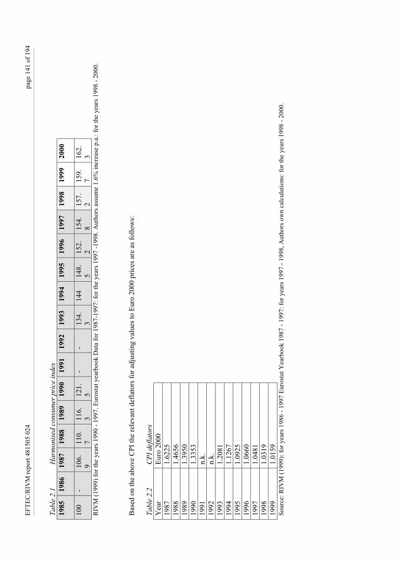
EFTE
C/R
IVM
repo
rt 48
1505
024
page
141
of 1
94
Tabl
e 2.
1H
arm
onise
d co
nsum
er p
rice
inde
x19
8519
8619
8719
8819
8919
9019
9119
9219
9319
9419
9519
9619
9719
9819
9920
00
100
-10
6.9
110.
711
6.3
121.
5-
-13
4.3
144
148.
515
2.2
154.
815
7.2
159.
716
2.3
RIV
M (1
999)
for t
he y
ears
199
0 - 1
997.
Eur
osta
t yea
rboo
k D
ata
for 1
987-
1997
: for
the
year
s 199
7 -1
998.
Aut
hors
ass
ume
1.6%
incr
ease
p.a
.: fo
r the
yea
rs 1
998
- 200
0.
Bas
ed o
n th
e ab
ove
CPI
the
rele
vant
def
lato
rs fo
r adj
ustin
g va
lues
to E
uro
2000
pric
es a
re a
s fol
low
s:
Tabl
e 2.
2CP
I def
lato
rsY
ear
Euro
200
019
871.
6225
1988
1.46
5619
891.
3950
1990
1.33
5319
91n.
k.19
92n.
k.19
931.
2081
1994
1.12
6719
951.
0925
1996
1.06
6019
971.
0481
1998
1.03
1919
991.
0159
Sour
ce: R
IVM
(199
9): f
or y
ears
198
6 - 1
997
Euro
stat
Yea
rboo
k 19
87 -
1997
: for
yea
rs 1
997
- 199
8, A
utho
rs o
wn
calc
ulat
ions
: for
the
year
s 199
8 - 2
000.

page
142
of 1
94EF
TEC
/RIV
M re
port
4815
05 0
24

EFTEC/RIVM report 481505 024 page 143 of 194
3. Valuing the risk of premature mortalityThe monetary estimates of the damage to human health from various pollutants and accidents tend todominate the total damage estimates. Therefore, it is useful to have a special section to make clear thedifferent concepts and methods for valuing the risk to human health.
For a change in risk that threatens life and health generally, the relevant valuation is the value that theindividual at risk attaches to their own health and life chances, plus what others would be willing topay to avoid the risk to that individual, plus any costs that society at large bears and which would nototherwise occur if the individual did not suffer the effects of the risk in question. The components ofthis value of risk (VOR) are:
(a) VORi,i where 'VOR' refers to the individual i's valuation of risk to themselves, i.e.'own risk'. The way in which these individual VORs are aggregated isdealt with shortly. Essentially, we will require the summation of such ownvaluations for all individuals at risk to give ΣiVORi,i, more commonlyknown as the 'value of a statistical life'
(b) VORi,j where the i,j notation now refers to j's valuation of risks to i. Again, thiswill need to be summed for all j, i.e. for all people expressing someconcern about risks to i, to give Σj VORi,j
(c) COIi where COI refers to the 'cost of illness' suffered by i but which costs areborne by the rest of society. An example would be hospital costs. COIcould be regarded as part of VORi,j
The relevant literature focuses on (a) with very limited evidence on (b). If the rule that individuals’preferences expressed as willingness to pay or accept is followed, then the component (c) should notbe included at the value of risk but expressed separately where relevant. Since the majority of valuesused in the literature as reported in this study are based on (a), the rest of this methodological sectionfocuses on this.
Valuing Statistical LivesThe way a VOSL is obtained is by aggregating up from a WTP value of risk reduction. Imagine theprobability of dying next year is 0.004 for each person and suppose we have 1000 persons in thepopulation. Assume there is some risk reduction policy that reduces the risk to 0.003, a change of0.001. Each person is asked to express their WTP for this change in risk and suppose the answer isEuro1000. The risk reduction policy is a public good: it affects everyone equally. Thus 1000 peoplesay they are each willing to pay Euro1000 for the policy, i.e. their aggregate willingness to pay isEuro1 million. The change in risk will result in one statistical person being saved each year (1000 x0.001). Thus the value of a statistical life is Euro1 million in this example. It is important tounderstand that no-one is being asked their WTP to avoid themselves dying at a specified time: theyare being asked to express a WTP for a change in risk.
Individuals' WTP to reduce risks can be expected to vary across different individuals. The two mainreasons for this will be that:
1. people have differing attitudes to risk: some may even be ‘risk lovers’, i.e. positively enjoyingrisky contexts. Most people are risk avoiders, i.e. they will tend to reveal a positive willingness topay for risk reduction. But there is no particular reason why their valuations of risk should be thesame;
2. incomes vary and hence willingness to pay is likely to vary in such a way that those with higherincomes have higher WTPs. This is not a necessary result since attitudes to risk may vary in such

page 144 of 194 EFTEC/RIVM report 481505 024
a way as to offset an income effect. Nonetheless, it raises an important equity issue about fairnessbetween people, an issue that is not in fact confined to risk valuations but to the use of WTPmeasures in general.
A VOSL can also be measured by a ‘willingness to accept’ compensation for increased risk. It is wellknown that many people do make this trade-off between risk and money, for example by acceptingpremia on wages to tolerate risk. It is tempting to think that the WTA approach will produce verymuch higher values for a VOSL than the WTP approach, simply because WTA is not constrained byincome. WTP and WTA can, indeed, be different and WTA for environmental losses may exceedWTP for environmental gains by factors of 2-5 (Gregory, 1986). Various explanations exist for thisdisparity, including the fact that individuals may feel they are losing an ‘entitlement’ if the issue isone of loss of an entitlement (WTA) rather than an increment to an existing entitlement (WTP).Another explanation, which is wholly consistent with economic theory, suggests that WTA > WTParises mainly in contexts where there is no ready substitute for the environmental good in question(Hanemann, 1991).
Table 3.1 presents the main valuation techniques used for estimating VOSL and the types of risks theymeasure based on the literature to date. Use of VOSL estimates of the kind noted in Table C1 hascome under criticism for several reasons:
• there is unease about the fact that health benefits based on VOSL are so dominant in cost-benefitstudies;
• the VOSL estimates come largely from accident contexts where the mean age of the person killedis very much lower than in pollution contexts. There is therefore a feeling that older people,perhaps with an already impaired health state will not have the same valuation of risk as someonewho is very much younger; and
• it is, as noted above, very easy to confuse what a VOSL is actually measuring. Wrongly translatedas a ‘value of life’, the concept is easy prey for critics who do not invest in attempts to understandthe analytical foundations of VOSL. Since this confusion is widespread, analysts often prefer notto use the VOSL concept at all.

EFTEC/RIVM report 481505 024 page 145 of 194
Table 3.1 Valuation techniques for measuring the risk to human healthMethod Scope CommentsHedonicwage(WTA)
Comparison of wage premiumbetween occupations with differentlevels of risks to human health.Values from literature range between£2.4 and 4.6 million
Other variables such as education,experience, the existence of unionsaffect the results; perception of risk ismore important than the actual levelof risk; evidence suggests thatworkers overstate the risk of theirjobs
Avertivebehaviour(WTP)
Measures the actual expenditure onsmoke alarms, safety harnesses,tamper-proof drug storage containersand other products that reduce the riskto human health. Values fromliterature range between £0.5-2.8million
In practice, finding examples ofavertive expenditure that are purelyto avoid risk to health has providedifficult
Contingentvaluation(WTP andWTA)
Respondents are asked how much theyare WTP or WTA to avoid or suffer amarginal change in the risk of dying.Values (WTP/A) from the literaturerange between £0.4-5.3 million
The responses are found to dependon the level and type of risk andwhether or not the respondent is in arisk group in addition to conventionalfactors such as income andeducation. Evidence shows thatinvoluntary risk such as cancer isvalued more highly than voluntaryrisk such as traffic accidents. Yet theempirical VOSL literature is almostentirely based on accident risks. Forpollution issues, then, transferringVOSLs from accident risk contextsto pollution contexts is likely tounderstate the 'true' degree of riskaversion.
Humancapitalapproach
What the person would have producedin the remainder of their lifetime net oftheir consumption – had they lived
The approach is inconsistent withWTP rule and is not used asextensively as before the WTP wasdeveloped
Of these reasons, only the second has any intellectual basis, although the first does reflect a 'statisticalsensitivity' issue in the sense that, if the VOSL estimates are wrong, then entire decisions may bechanged.
For these good and bad reasons, then, there have been attempts to estimate not the value of the risk offatality but the value of the life period gained by reducing the risk. This has come to be known as the'value of a life year' or VOLY.
Value of a Life Year (VOLY)The underlying rationale for valuing ‘life years’ is that many contexts in which health risks occurrelate to pollution. Clearly, pollution is more likely to affect people who are most vulnerable. In apoor country this may be the very young and the very old. In a rich country, where infant mortalityrisks are very low, it is more likely to affect the elderly and especially those who are already at risk

page 146 of 194 EFTEC/RIVM report 481505 024
from their prevailing health state. Suppose, for argument's sake, that, statistically, the reduced lifeexpectancy of someone exposed to air pollution is six months. Then, the argument goes, what mattersis the value the individual places on those six months of extended life. If the period is a few weeks oreven days, then the relevant value is that ‘life period’ rather than the actual risk.
This contrasts with the VOSL where a person, however old they are, is faced with a risk and theyexpress their WTP to reduce that risk. In principle, the two values - VOSL and VOLY - should bearsome relationship since the person at risk must have some idea of remaining life expectancy. Indeed,it would be extremely surprising if they did not. In expressing a WTP to reduce risk, then, they shouldbe accounting for the remaining life period available to them.
One obvious way of approaching the problem is to see if WTP to reduce risks is functionally relatedto age, an issue we return to below. The surprising thing about the VOSL literature is that very little ofit controls for age, so that only a few studies exist to offer a guide on how risk valuations vary withage.
Alternative approaches attempt to estimate the VOLY and, so far, two procedures have been used.The first simply takes estimates of the VOSL and converts them to values of life year; i.e. noadditional information is sought. The second attempts to construct VOLY from first principles byengaging in valuation studies that directly attempt to elicit the WTP for extended periods of life.
VOLY derived from VOSLOne approach to estimating the VOLY is to regard it as the annuity which when discounted over theremaining life span of the individual at risk would equal the estimate of VOSL.
VOLY = VOSL/A
where A = [1-(1+s)-T]/s and T is years of expected life remaining and s is the utility discount rate20.
While the VOLY approach may appear sound, it offers no evidence that VOSL declines with age inthe manner shown. If this were to be the case, we would expect to find evidence that the WTP toreduce risks varies inversely with age. As Rowlatt et al. (1998) note, there is some evidence for adeclining WTP as people become older, but that evidence is not at all consistent with the age profileof VOSL as dictated by the VOLY approach. Maddison (1998) suggests that there are sound reasonsfor supposing that VOSL is proportional to the number of discounted life years remaining to anindividual and that it is inversely proportional to the survival probability in the current time period. Inother words, Maddison suggests that there are rationales for a declining VOSL with age, but that thiswill be attenuated in old people by the reduced survival probability. For the UK, he suggests that theVOSL for a 74-year-old with six months life expectancy would be 17% of the healthy 36-year-old.
However, to quote a study for the US Environment Protection Agency:
‘..it is possible that the reduced life expectancy and reduced enjoyment of life associated with manychronic illnesses may result in lower WTP to reduce risks of death. On the other hand, facing seriousillness and reduced life expectancy may result in higher value [being] placed on protecting theremaining time.’ (Chestnut and Patterson, 1994) .
Overall, Maddison’s approach holds out some promise for finding age-related VOSLs via indirectroutes. These should then be tested against VOSLs derived from direct approaches in which age isspecifically accounted for.
20 The utility discount rate is the rate at which future wellbeing is discounted, not the rate at which income or
consumption is discounted.

EFTEC/RIVM report 481505 024 page 147 of 194
VOLY derived from WTP experimentsAn alternative procedure based on the VOLY concept is to see the WTP to extend a lifetimeconditional on having reached a certain age. There is only one such study to date (Johannesson andJohansson, 1996) that reports a contingent valuation study in Sweden that measured people’spreferences for one extra life year at the age of 85. The results suggest average WTP across the agegroups of slightly less than 10,000 SEK using standard estimation procedures and 4,000 SEK using amore conservative approach. In dollar terms this is $600-1500. Recall that this is for one year ofexpected life increase. WTP actually increases with age, although not dramatically - on the standardbasis, 8000 SEK for the 18-34 age group, 10,000 for the 35-51 age group and 11700 for the 51-69 agegroup. Using the formula:
VOSL(a) = VOLY.Σ 1/(1+s)T-a
Where T is life expectancy and a is the age at which VOSL is measured. Johannesson and Johanssonsuggest these values are consistent with 'normal' VOSL of $30,000 to $110,000, substantially lessthan the VOSL derived previously. Since T-a is obviously less the older the age group, then therelevant VOSL will decline with age. They also derive discount rates of 0.3% to 3.4% and these areinvariant with age.
Finally, they argue that these lower valuations are consistent with findings in Sweden and the USA onsocial attitudes to allocating resources to life saving. Thus, Cropper et al (1994) found that surveyrespondents strongly favoured life saving programmes which save the lives of young people ratherthan old people. Earlier work by Johannesson and Johansson (1995a, 1995b) found that Swedishattitudes were similar, and that expectations about the future quality of life at old age play asignificant role (regardless of what the actual quality of life is). The implications of the low WTPvalues for health care are hinted at in Johannesson and Johansson (1996): they observe that the VOSLvalues are ‘negligible’ compared to the costs of health treatment for the aged.
Is the WTP approach used in the Johannesson and Johannsson study consistent with the VOSLapproach ? It is arguable that the ‘goods’ being valued are quite different: VOSL studies value riskand the VOSL is simply an aggregation of those individual valuations of risk. The WTP for a life yearis not explicitly a value of risk, but a value of extending a life year once the respondent is assumed toreach a particular age. The Johannesson and Johansson paper could be argued to be more relevant forpollution control policy if the benefits of that policy are thought to accrue mainly to the elderly.
ConclusionsFew topics have proved so controversial as the ‘value of statistical life’. In large part the controversyderives from unfortunate terminology, since what appears to be at stake is the 'value of life' itself. Thisconfusion has not been helped by even the most distinguished commentators and analysts using thisphrase. But what is being estimated is the value of risk reduction. VOSL is essentially, a convenientway of aggregating these estimates.
In a finite world there really should be no dispute that resources have to be allocated rationally acrossdifferent life risks. The real focus of the debate should be on the size of the VOSL. As we saw, this isthe subject of a debate, which centres on two approaches to valuing risks. The first asks for the WTPto avoid risks, and the second asks for the WTP to extend an expected lifetime by some finite period,say, one year. The literature on ‘value of life year’ turns out to be a hybrid of these approaches,deriving VOLY from a given VOSL. As discussed, there appears to be limited theoretical justificationfor this hybrid approach. It is also not consistent with what we know about VOSL as they vary withage. Nonetheless, what we know about the age-WTP relationship is not much. In turn, the literaturethat attempts directly to estimate VOLY is minute. Such as it is, it suggests VOSL are very much lessthan those derived from standardised value of risk calculations.

page 148 of 194 EFTEC/RIVM report 481505 024
Other issues concern the role that others' valuation of risks should play and the role that discountingmight play in valuing future risks. In general it would appear that there is a case for adding a modestpremium to own VOSL for others' altruistic concerns, and there is no strong case for discountingfuture risks.
Finally, note that majority of the studies estimating the economic cost of air pollution damage tohuman health that are reported in this study use the VOSL approach.
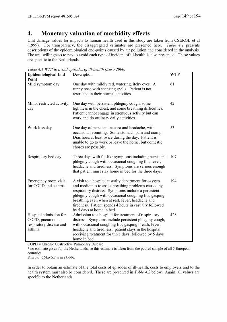
EFTEC/RIVM report 481505 024 page 149 of 194
4. Monetary valuation of morbidity effectsUnit damage values for impacts to human health used in this study are taken from CSERGE et al(1999). For transparency, the disaggregated estimates are presented here. Table 4.1 presentsdescriptions of the epidemiological end-points caused by air pollution and considered in the analysis.The unit willingness to pay to avoid each type of incident of ill-health is also presented. These valuesare specific to the Netherlands.
Table 4.1 WTP to avoid episodes of ill-health (Euro,2000)Epidemiological EndPoint
Description WTP
Mild symptom day One day with mildly red, watering, itchy eyes. Arunny nose with sneezing spells. Patient is notrestricted in their normal activities.
61
Minor restricted activityday
One day with persistent phlegmy cough, sometightness in the chest, and some breathing difficulties.Patient cannot engage in strenuous activity but canwork and do ordinary daily activities.
42
Work loss day One day of persistent nausea and headache, withoccasional vomiting. Some stomach pain and cramp.Diarrhoea at least twice during the day. Patient isunable to go to work or leave the home, but domesticchores are possible.
53
Respiratory bed day Three days with flu-like symptoms including persistentphlegmy cough with occasional coughing fits, fever,headache and tiredness. Symptoms are serious enoughthat patient must stay home in bed for the three days.
107
Emergency room visitfor COPD and asthma
A visit to a hospital casualty department for oxygenand medicines to assist breathing problems caused byrespiratory distress. Symptoms include a persistentphlegmy cough with occasional coughing fits, gaspingbreathing even when at rest, fever, headache andtiredness. Patient spends 4 hours in casualty followedby 5 days at home in bed.
194
Hospital admission forCOPD, pneumonia,respiratory disease andasthma
Admission to a hospital for treatment of respiratorydistress. Symptoms include persistent phlegmy cough,with occasional coughing fits, gasping breath, fever,headache and tiredness. patient stays in the hospitalreceiving treatment for three days, followed by 5 dayshome in bed.
428
COPD = Chronic Obstructive Pulmonary Disease* no estimate given for the Netherlands, so this estimate is taken from the pooled sample of all 5 Europeancountries.Source: CSERGE et al (1999).
In order to obtain an estimate of the total costs of episodes of ill-health, costs to employers and to thehealth system must also be considered. These are presented in Table 4.2 below. Again, all values arespecific to the Netherlands.

page 150 of 194 EFTEC/RIVM report 481505 024
Table 4.2: Productivity and health service costs for ill-health (Euro, 2000)Per diem productivity cost (Euro/day) 64Emergency room visit (Euro/visit) 45Hospitalisation (Euro/inpatient day) 367Source: CSERGE et al (1999).
Table 4.3 uses the values presented in Tables 4.1 and 4.2 above to derive the total cost of an episodeof ill-health of each given type.
Table 4.3 Total costs of episodes of ill-health (Euro, 2000)Epidemiological EndPoint
WTP Productivitycosts
ERV costs Hospitalisationcosts
Total costs
Symptom day 61 - - - 61MRAD 42 - - - 42Work loss day 53 64 - - 117Respiratory bed day 107 192 - - 299Emergency room visit 194 320 45 - 559Hospital admission 428 320 - 367 1,115Source: CSERGE et al (1999).
In the sensitivity analysis, the effects of using different values for these epidemiological endpoints istested. Monetary valuation estimates are taken from ExternE (1998). These are summarised in Table4.4 below.
Table 4.4 Monetary valuation estimates used in the sensitivity analysisImpact Unit value
(Euro, 2000)Reference (estimation method)
Mortality 0 – 65 years 4.98 CSERGE et al, 1999Mortality +65years 3.49 adjusted from CSERGE et al, 1999
(using results of Pearce, 1997)Respiratory hospital admission(RHA)
8,304 – 8,853 Maddison, 1997 (adjusted COI) - Markandya,1997 (CV)
Emergency room visit (ERV) 42 – 251 Maddison, 1997 (adjusted COI) – Markandya,1997 (CV)
Restricted activity day (RAD) 20 – 85 Maddison, 1997 (adjusted COI) – Markandya,1997 (CV)
Respiratory symptoms (SD) 5 - 9 Maddison, 1997 (CV) – Markandya, 1997 (CV)

EFTEC/RIVM report 481505 024 page 151 of 194
5. Environmental data, assumptions and modelsFor the benefit analysis we used the most recent data available. We present data for the current statusof each environmental issue (1995) and the expected future progress (2010, 2020 and 2030). Data areexpressed as tonnes of emissions of each pollutant, concentrations and/or exposure levels. The dataare drawn from the (draft) Fifth National Environmental Outlook for the Netherlands (NEO5). Thisreport is prepared for the Fourth Dutch Environmental Policy Plan (to be published in the beginningof 2001).
The aim of NEO5 is to assess the state of the environment in the view of sustainable development inthe Netherlands and in its international context. The NEO5 includes an appraisal of the nature andcauses of the persistent environmental problems in the Netherlands, and it inventorises new emergingissues. The appraisal of the persistency of environmental problems is based on historicalenvironmental data in relation to current policies (for the period 1970-2000) and also on futuredevelopments.
The following persistent environmental problems can be listed:
• climate change;• acidification including tropospheric ozone;• particulate matter;• eutrophication, and• noise disturbance. Scenario and current legislation Future progress of the environmental issues has been based on future societal trends. As these trendsare in principal uncertain we have to apply scenarios. For this study we have only used one scenario,as the focus of the study is on ranking of the environmental issues. This ranking is unlikely to beaffected by the scenario choice. For our study we have chosen the so-called European Co-ordinationscenario (CPB, 1997). Characteristics of the scenario are the following: • the rise of ‘Fortress America’ and the tendency toward strategic trade and industrial policies
significantly contribute to formation of trade blocks;
• despite increasingly strained relations with the USA, Western Europe develops very favourably.The European process of integration is an important stimulus toward strengthening incentivestructures on the Western European product and labour markets. A far-reaching process of reformof the West European welfare state is set in motion. In this, attempts are made to combine theEuropean tradition of social equity, with an increased sensitivity to economic incentives;
• the EU introduces an energy/carbon tax of $ 10 per barrel;
• Technological development and diffusion is moderate;
• There is high migration to the EU. Some key figures of EC scenario are presented in Table 5.1.

page 152 of 194 EFTEC/RIVM report 481505 024
Table 5.1 EC scenario key figures 1995 2020 Population (million) 15.5 17.7 Number of households (million) 6.5 4.5 Consumption per capita (index) 100 170 GDP growth (index) 100 195 Oil price ($ per barrel) 17 25 The societal trends of the EC scenario have been combined with the environmental policies already inplace in the Netherlands21 and the EU. This is referred to as the 'current legislation scenario' (CLS). The following key environmental policies are included in CLS: • Climate change policy plan (1999); implementation of Kyoto protocol;• European emission directives (e.g., EURO IV);• Most recent emission standards for combustion;• Integrated policy plan for reducing ammonia and manure , and• Most recent noise standards for transport. Models and data flows The results of the Fifth National Environmental Outlook will be published in July 2000. Allenvironmental data (indicators) used in this report will be fully documented in so-called factsheets.These factsheets will contain the following: • data source (RIVM or other);• data consistency check;• description of the indicator;• computation (model name, version, spreadsheet);• data uncertainty;• data input and assumptions, and• references.
The justification of the data input for the benefit estimations can be found in these factsheets. Theannex of this report shows the main data flows of the NEO5 (in Dutch), (see Annex I.6).
General data used in this study are presented in Table 5.2.
Table 5.2 General data used in this studyData 1995 2010 2020 2030Population: millions 15.424 16.821 17.673 18.406Size of households 2.34 2.27 2.23 2.21GDP: Euro billion 312.6273 482.5431 632.9282 830.1809
Environmental dataThe following tables present the environmental data used in this study. The data are provided byRIVM and are taken from the 5th National Environmental Outlook, (draft report), with the exceptionof land contamination, which is not discussed in that report.
21 Policies in place as approved by the Dutch parliament before January 1, 2000

EFTEC/RIVM report 481505 024 page 153 of 194
Climate changeTable 5.3 presents the greenhouse gases emitted from the Netherlands.
Table 5.3 Gases contributing to climate change: current legislation scenarioCarbon dioxide, CO2: million tonnes
1995 2010 2020 2030waste management 1.5 2.0 2.0 2.0Construction 0.7 0.8 0.8 0.8Households 21.8 21.5 20.0 18.3water 0.0 0.0 0.0 0.0energy 45.9 47.5 50.0 57.1Services 9.9 13.5 15.3 16.7Industry 44.3 45.2 49.3 53.7Agriculture 9.4 10.4 11.0 11.6Other 2.5 3.0 3.0 3.0Refineries 11.5 15.6 17.0 17.8sewage treatment 0.1 0.1 0.1 0.1Transport 32.4 38.7 44.5 52.2Total 180.2 198.3 213.1 233.3Methane, CH4: thousand tonnes
1995 2010 2020 2030waste management 479 217 102 51Households 18 16 16 16energy sector 178 73 38 38Industry 8 5 5 6Agriculture 479 385 368 343Other 5 5 5 5Transport 6 3 2 2Total 1172 703 537 462Nitrous dioxide, N2O: thousand tonnes
1995 2010 2020 2030energy sector 0.4 0.2 0.1 0.1Industry 31.7 32.9 34.2 35.8Agriculture 27.6 20.9 20.0 19.6Other 5.0 5.0 5.0 5.0Transport 7.1 2.6 2.2 2.6Total 71.9 61.6 61.5 63.1Total per gas (million tonnes CO2-eq)CO2 180.2 198.3 213.1 233.3CH4 24.6 14.8 11.3 9.7N2O 22.3 19.1 19.1 19.6HFK 6.7 3 5.4 6.5PFC 2.1 0.9 1.1 1.2SF6 1.5 2.0 2.3 2.7Total (IPCC) 237.3 238.1 252.2 273.0Source: Fifth National Environmental Outlook (draft report).

page 154 of 194 EFTEC/RIVM report 481505 024
AcidificationTable 5.4 presents the acidifying pollutants emitted from the Netherlands.
Table 5.4 Gases contributing to acidification: current legislation scenarioAmmonia, NH3: 1000 tonnes
1995 2010 2020 2030Households 6.7 7.4 7.8 8.2Industry 4.1 4.1 4.3 4.7Agriculture 176.9 143.0 133.4 128.0Other 0.6 0.7 0.8 0.8Total 188.4 155.2 146.3 141.7Nitrogen oxides, NOx: 1000 tonnesHouseholds 22.3 14.4 12.0 9.8Energy 58.1 23.8 25.4 25.4Services 8.1 7.6 7.4 7.0Industry 61.2 42.5 42.2 42.2Agriculture 10.3 12.0 9.5 7.5Other 3.8 2.4 2.6 2.6Refineries 17.7 8.1 8.2 8.2Transport 313.1 161.2 149.3 173.5Total 494.6 272.1 256.6 276.2Sulphur dioxide, SO2: 1000 tonnesWaste 0.5 0.3 0.3 0.3Energy 16.7 9.8 8.6 10.5Industry 29.8 23.8 24.7 25.7Other 5.7 2.7 2.8 2.8Refineries 61.2 21.0 22.0 22.3Transport 29.9 13.7 15.4 17.2Total 143.8 71.2 73.8 78.6Source: Fifth National Environmental Outlook (draft report).
Low level ozoneTable 5.5 presents VOC emissions that contribute to low level ozone in the Netherlands. NOxemissions are given in Table 5.4. Table 5.6 reports the ill-health incidences associated with exposureto low level ozone. The dose response functions used to derive the ill-health incidences are reported inthe appendix to Section 4.7.
Table 5.5 VOC emissions: current emissions scenario: 1000 tonnesSource 1995 2010 2020 2030Transport 148.3 51.9 48.4 52.4Industry 80.9 55.4 59.5 63.6Households 39.6 31.1 33.7 37.7Services 29.2 18.7 20.8 23.1Energy 26.2 15.8 13.8 13.8Construction 21.9 10.5 11.8 12.1Refineries 11.7 9.0 9.0 9.0Other 4.0 2.4 2.2 2.1Total 361.8 194.9 199.2 213.7Source: Fifth National Environmental Outlook (draft report).
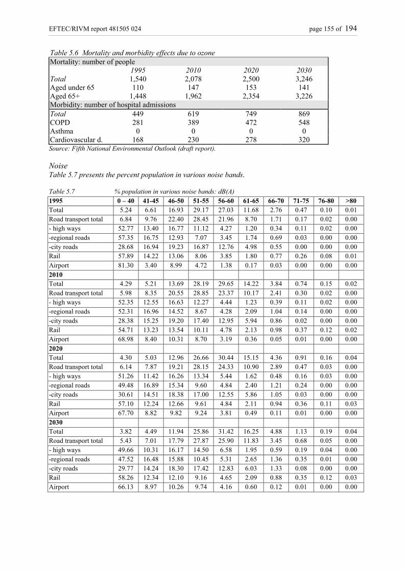
EFTEC/RIVM report 481505 024 page 155 of 194
Table 5.6 Mortality and morbidity effects due to ozoneMortality: number of people
1995 2010 2020 2030Total 1,540 2,078 2,500 3,246Aged under 65 110 147 153 141Aged 65+ 1,448 1,962 2,354 3,226Morbidity: number of hospital admissionsTotal 449 619 749 869COPD 281 389 472 548Asthma 0 0 0 0Cardiovascular d. 168 230 278 320Source: Fifth National Environmental Outlook (draft report).
NoiseTable 5.7 presents the percent population in various noise bands.
Table 5.7 % population in various noise bands: dB(A)1995 0 – 40 41-45 46-50 51-55 56-60 61-65 66-70 71-75 76-80 >80Total 5.24 6.61 16.93 29.17 27.03 11.68 2.76 0.47 0.10 0.01Road transport total 6.84 9.76 22.40 28.45 21.96 8.70 1.71 0.17 0.02 0.00- high ways 52.77 13.40 16.77 11.12 4.27 1.20 0.34 0.11 0.02 0.00-regional roads 57.35 16.75 12.93 7.07 3.45 1.74 0.69 0.03 0.00 0.00-city roads 28.68 16.94 19.23 16.87 12.76 4.98 0.55 0.00 0.00 0.00Rail 57.89 14.22 13.06 8.06 3.85 1.80 0.77 0.26 0.08 0.01Airport 81.30 3.40 8.99 4.72 1.38 0.17 0.03 0.00 0.00 0.002010Total 4.29 5.21 13.69 28.19 29.65 14.22 3.84 0.74 0.15 0.02Road transport total 5.98 8.35 20.55 28.85 23.37 10.17 2.41 0.30 0.02 0.00- high ways 52.35 12.55 16.63 12.27 4.44 1.23 0.39 0.11 0.02 0.00-regional roads 52.31 16.96 14.52 8.67 4.28 2.09 1.04 0.14 0.00 0.00-city roads 28.38 15.25 19.20 17.40 12.95 5.94 0.86 0.02 0.00 0.00Rail 54.71 13.23 13.54 10.11 4.78 2.13 0.98 0.37 0.12 0.02Airport 68.98 8.40 10.31 8.70 3.19 0.36 0.05 0.01 0.00 0.002020Total 4.30 5.03 12.96 26.66 30.44 15.15 4.36 0.91 0.16 0.04Road transport total 6.14 7.87 19.21 28.15 24.33 10.90 2.89 0.47 0.03 0.00- high ways 51.26 11.42 16.26 13.34 5.44 1.62 0.48 0.16 0.03 0.00-regional roads 49.48 16.89 15.34 9.60 4.84 2.40 1.21 0.24 0.00 0.00-city roads 30.61 14.51 18.38 17.00 12.55 5.86 1.05 0.03 0.00 0.00Rail 57.10 12.24 12.66 9.61 4.84 2.11 0.94 0.36 0.11 0.03Airport 67.70 8.82 9.82 9.24 3.81 0.49 0.11 0.01 0.00 0.002030Total 3.82 4.49 11.94 25.86 31.42 16.25 4.88 1.13 0.19 0.04Road transport total 5.43 7.01 17.79 27.87 25.90 11.83 3.45 0.68 0.05 0.00- high ways 49.66 10.31 16.17 14.50 6.58 1.95 0.59 0.19 0.04 0.00-regional roads 47.52 16.48 15.88 10.45 5.31 2.65 1.36 0.35 0.01 0.00-city roads 29.77 14.24 18.30 17.42 12.83 6.03 1.33 0.08 0.00 0.00Rail 58.26 12.34 12.10 9.16 4.65 2.09 0.88 0.35 0.12 0.03Airport 66.13 8.97 10.26 9.74 4.16 0.60 0.12 0.01 0.00 0.00

page 156 of 194 EFTEC/RIVM report 481505 024
Land contamination
Table 5.8 gives the number of contaminated sites in the Netherlands in and their distributions amongstland use types (1996 figures) and the distribution of land uses when all contaminated sites are cleaned.The table also shows the size (ha) of contaminated sites both for 1996 (all contaminated) and for thetime when all contaminated land is cleaned.
Table 5.8 Contaminated areasContaminated Land Cleaned Land
No. of sites Land area (ha) No. of sites Land area (ha)Total 351,000 631,800 351,000 631,800Residential 91,228 164,210 150,000 269,993Industrial 126,328 227,390 90,768 163,384Agricultural 41,084 73,953 39,430 70,970Recreationaland nature
23,292 41,926 26,676 48,017
Derelict 29,600 53,280 4,696 8,453Dumping 7,925 14,267 2,179 3,924Other 31,540 56,774 37,248 67,046Source: RIVM, 1997 Achtergronden bij: Milieubalans 1997, Samson HD, Tjeenk Willink Alhen aan de Rijn.
Particulate matterTable 5.9 reports emissions of PM10, whilst Table E10 gives the associated ill-health incidences. Thedose response figures used to determine ill-health incidences are given in the appendix to Section 4.5.
Table 5.9 PM10 emissions: current legislation scenario: 1000 tonnes1990 2010 2020 2030
Consumers 6.8 6.5 6.6 6.7Energy sector 0.6 0.4 0.3 0.3Industry 14.3 7.9 8.2 8.4Other 1.3 0.7 0.7 0.2Refineries 4.8 2.0 1.8 1.8Transport 18.6 9.9 9.8 11.0TOTAAL 46.4 27.5 27.4 28.4Source: Fifth National Environmental Outlook (draft report).
Table 5.10 Mortality and morbidity effects due to PM10: current legislation scenarioMortality (number of people)
1995 2010 2020 2030Total 931 992 1172 1529Aged under 65 135 147 152 142Aged 65+ 796 845 1020 1387Morbidity (number of hospital admissions)TotalCOPDAsthmaCardiovascular disease
36089581331214
3597953122
1240
43991161129
1576
53201401136
1963Source: Fifth National Environmental Outlook (draft report).

EFTEC/RIVM report 481505 024 page 157 of 194
EutrophicationTable 5.11 gives the nitrogen and phosphorus emissions from the Netherlands.
Table 5.11 Nitrogen and phosphorus emissions: current legislation scenarioN: 1000 tonnes
1996 2010 2020 2030Total emissions 56 33 33 33Domestic effluent 35.06 21.84 22.81 23.46Agriculture 6.27 0.92 0 0Industry 5.70 3.80 3.80 3.80Atmospheric deposition 5.62 4.21 4.01 3.88Sewage 1.20 0.98 0.93 0.88Overflow 1.09 0.97 0.88 0.87Households not connected 0.69 0.23 0.23 0.23P: 1000 tonnesTotal emissions 7.6 3.5 3.6 3.6Industry 3.55 0.66 0.66 0.66Domestic effluent 3.36 2.64 2.73 2.80Overflow 0.12 0.09 0.11 0.11Households not connected 0.11 0.07 0.07 0.07Agriculture 0.44 0.03 0.01 0.00Source: Fifth National Environmental Outlook (draft report).

page 158 of 194 EFTEC/RIVM report 481505 024

EFTEC/RIVM report 481505 024 page 159 of 194
159
6. Data flows of the 5th National Environmental Outlook
Environmental Pressures and the Calculation of EmissionsThe main environmental pressures on health and nature are considered to be climate change, long-range air pollution (acidification and smog), eutrophication and urban stress (noise and urban airquality). Analysis of the environmental pressure exerted by the economic sectors relevant to theseenvironmental themes is the chief responsibility of the RIVM, both for the annual EnvironmentalBalances and for the Environmental Outlooks, making use of the relevant input data, scenarios,environmental policy and technological developments. The developments given in the socioeconomicscenarios are translated into emissions to the environment. Figure 2.1 below shows the generalfeatures of this process.
The most basic formula for determining all emissions can be reduced to the following:
E = V (economy-, demography- and policy-related) * K (technology, policy)where:E = EmissionV = Volume (e.g. industrial production volume, transport volume in tonne kilometres, animal
stock, etc.)K = Emission factor per Unit Volume.
The formula above is used at all relevant sub classification levels of production sectors andconsumption categories, adding up to total Dutch production and consumption figures on a nationalscale.
Volume indicatorThe first perhaps most relevant step in the calculations is to derive the environmentally relevantvolume-indicators V. Volumes of production or consumption are a function of economic and/ordemographic parameters as given in the economic scenarios and human behaviour. This combinationis sometimes performed using econometric models with underlying price elasticity studies etc., withthe relevant volume-indicators as output results.
An example is the traffic model FACTS 3.0 (Forecasting Air pollution by Car Traffic Simulation).This flexible model, originally developed by the Netherlands Economic Institute, draws up forecastsof car ownership and use as well as their emissions and energy consumption, all under alternativescenarios of economic and demographic development, emission regulation, fuel efficiency, prices offuels and cars, and other government measures relating to traffic and transport.
Many of the policy and other model parameters can be varied, for instance economic development,demographic evolution, developments in fixed and variable car costs, and levels of emission andenergy consumption.
In other cases, specific data necessary for the calculation are not available. In that case the estimationand prediction of volumes is based on the historical relationship between monetary data andemissions. Where relevant, the influence of environmental policy is also taken into consideration,resulting in generally accepted restrictive measures. These measures involve limitation of the increasein livestock as a consequence of policy measures, the influence on traffic and transport, etc.

page 160 of 194 EFTEC/RIVM report 481505 024
Financial and/or Emitting Emissions Contribution toPhysical Volume of Processes Env. Theme
such as such asEconomydisposable incomeemploymenttechnology
Industrial productionstructure of industrymaterial flowsdematerialisation and upgrading
Chemicalprocesses
CO2, SO2NOx
Agricultural productionstructure of agriculturegreenhouse cultivationstock breeding
Distributingmanure
P2O5, N,NH3, CH4 Air and Water
Pollution
Transport productiontransport sectorpassenger trafficaviation
Petrol / dieselengines
Noise, NOxPM10CO2
Eutrophication
Urban Stress
Consumptionconsumption patternsGDP and private consumptionspending on transport
Domesticheating
CO2NOx
Climate Change
Energy supply andconsumptionconsumption per personconsumption per target groupenergy supplyenergy prices
Burning fossilfuels
CO2
Land useagricultural acreageacreage of nature areasbuilt-up areainfrastructure
Depositionofpollutants
EcologicalEffects
Ref
eren
ce S
cena
rio
Populationpopulation densityage categorycomposition of familyhousing stock
Exposuretopollutants
HealthEffects
Additional environmental policy (in so far as not included in reference scenario)pricing policy, policy on levies, technology policy, covenants
Figure 2.1 Chart for calculating emissions
EFTEC/RIVM report 481505 024 page 161 of 194
161
Emission factorsEmission factors K (per Unit of Volume) are influenced by technological developments and the waythese developments are affected by policy measures.
• Technological development Technological development plays an important role in the link between physical production andresulting emissions and is seen by the Dutch government as an important instrument in improvingenvironmental quality and avoiding economic harm. RIVM’s inventory of technologicaldevelopments and their impacts on emission factors is based on both studies of the literature andexpertise in the field of application. Prognoses up to 2020 mainly involve conventional technology.Detailed information on technology and implementation grades is aggregated to annual averages. Forprognoses from 2020 up to 2030 more aggregated assumptions are made and more radical changesand breakthrough technologies are taken into consideration.• Environmental policyThe reference scenario in the 5th Environmental Outlook is based on all ‘agreed policy measures’.‘Agreed policy measures’ are defined as ‘all government-endorsed policy instruments translated intoreal technological or other measures to be implemented in the various sectors of industry, agriculture,etc.’. A draft list of these instruments/measures is communicated to and discussed with policymakersto obtain consensus and avoid misunderstanding.If certain agreed policy results receive very low public and/or interdepartmental support andimplementation proves to be doubtful, margins in their environmental effects are given by presentingboth calculation results.• SpecificIf no more widely accepted specific scenarios are available, e.g. on lifestyle, consumer behaviour,technical developments, etc., expert judgement teams are invited to participate in a broad debate inorder to obtain the largest possible consensus for specific scenarios.
UncertaintiesIn calculating trends in volumes and emission factors uncertainties cannot be avoided. Therefore,scenario data contain margins or a bandwidth. Future implementation grades e.g. have to beestimated, using knowledge of present state-of-the-art technology and the tendency to technologicalinnovation in the sectors in the future.It turns out that uncertainties in policy implementation can have as much impact on the outcomes aseconomic uncertainties, sometimes even more.In addition to the reference scenario, additional policy options are defined in close collaboration withpolicymakers and their effects are estimated by calculation. The results obtained form the input for theNational Environmental Policy Plan.

page 162 of 194 EFTEC/RIVM report 481505 024

EFTEC/RIVM report 481505 024 page 163 of 194
163
Annex II Integrating cost-benefit analysis into thepolicy process
by
Professor David PearceDepartment of Economics, University College London
with
Economics for the Environment Consultancy Ltd (EFTEC)

page 164 of 194 EFTEC/RIVM report 481505 024

EFTEC/RIVM report 481505 024 page 165 of 194
165
1. Purpose of the paperThis paper is concerned with the issue of how to introduce more rational procedures into publicdecision-making. It is a non-technical paper, written in the belief that there is still scope to improvethe ways in which politicians, civil servants, experts, advisers and the community at large currentlymake decisions. Exactly what is meant by ‘improving’ decision-making will become clear as we goalong. The focus is on economics, improving decision-making by using economics and whyeconomists have some special insights to offer. Economists are not alone in having thought about theprinciples of better decision-making. However, others will be better placed to give advice on howother disciplines can improve decision-making.
The paper is structured as follows:
(a) we begin with the logical structure of rational decision-making (RDM), focusing on analternatives-criteria matrix familiar in policy analysis. The alternatives-criteria matrix is thebasis upon which all interested parties can have discourse about decision-making. This discourseis the essential basis for introducing RDM into decision-making procedures. In particular, wefocus on cost-benefit analysis. We argue that cost-benefit analysis (CBA) is a comprehensiveRDM which does, however, focus on the notion of economic efficiency. In so far as otherobjectives are relevant to decision-making, CBA will be a necessary but partial input tocomprehensive decision-making.
(b) getting a discourse under way also involves addressing the baseline issue, i.e. what would happenif a given RDM procedure is not used and some other procedure is used instead.
(c) countries differ in the extent to which they employ rational decision making procedures and it isan interesting question as to why this is the case. We address this issue also since it casts somelight on how procedures for enhancing the use of RDM can be implemented.
(d) we also look at the issue of what to do if a given RDM cannot be implemented fully because oftechnical or data difficulties. In particular, we ask what should be done when monetised costs andbenefits can be estimated for some, but not all, effects of a policy or a project.
(e) While there are many technical issues relating to the validity or otherwise of CBA, a particularone has been highlighted by the steering committee for this paper: how to set the geographicalboundaries of costs and benefits. We address this issue directly.
(f) Finally, we look at some strategic matters relating to the process for introducing RDMprocedures. Of necessity, strategy will vary with the political and institutional contexts, sogeneralisations are difficult. Nonetheless, we suggest there are some basic rules that might befollowed by those who wish to advance RDM procedures in government.
We conclude that CBA is a powerful RDM tool. It is not without problems but the issue is whetherthose problems render its results invalid, and whether the results could be improved upon by adoptingother RDM techniques. We argue that other techniques have as many, if not more, drawbacks asCBA.

page 166 of 194 EFTEC/RIVM report 481505 024
2. The issue: how to introduce rationality in public decision-making
The first issue to be addressed is the context for rational discourse about how to make decisions.Unless the ground rules for having this discourse are agreed, most argument and advocacy will befruitless. Experience with decision-making suggests that most people would agree certain groundrules, even if they would want to stress some criteria for RDM over others.
All public decision-making involves choice. The necessity of choice arises because public funds arelimited. Resources allocated to one purpose cannot be used to fund a different purpose. Money is ameasure of resource use. Money spent on, say, education, cannot be spent on health care or theenvironment. Hence choices, or trade-offs, have to be made. To the economist, the inevitability ofmaking choices is what defines the subject matter of economics. The value of the option that issacrificed when a particular choice is made is known as the opportunity cost. If A is chosen over B,the opportunity cost is the lost benefit from B. While it may seem redundant to remind decision-makers that all their decisions involve an opportunity cost, professionally-trained people often do notbehave as if there is a sacrifice when they make choices. The reality is that they probably doappreciate there are opportunity costs. What they are more likely to be saying is that their use of theresources is more valuable to society than the alternative use of the resources. The librarian will arguethat spending money on libraries is vitally important. The medic will invoke the value of saving livesto justify more spending on medicine. The media will express outrage that a particular drug is notavailable on demand simply because it is very expensive. The schoolteacher will speak of the specialneeds of children and of education for the future. Each may speaks of ‘rights’ to information, health,education and so on. But in a finite world, there are no absolutes. Some things are indeed veryimportant, but nothing is so important that it justifies allocating all of society’s resources to it, nordoes any society behave that way. Because the subject matter of economics is defined as makingchoices in the context of finite resources, economists have a lot to say about how to choose betweenalternative uses of resources. That does not mean that economists alone should give guidance on howto choose. All disciplines have something to offer in terms of this guidance, but it seems fair to saythat economic advice is very important precisely because economists have a discipline which isdefined by this issue of how to make choices.
To the economist, rational choice means making the ‘best’ use of available resources. The focus ismainly on a nation’s resources, because those are the resources over which national decision-makershave some control. But the principles of rational choice are just as applicable to resources beyondnational frontiers. By engaging in international agreements, for example, nations effectively makesome claim to determining choices that relate to the resources of other nations. But what is the ‘best’use of resources?
‘Best’ is a value word. That means that what is best depends on what the objective is that we chooseto try and achieve. In turn, there can be many different, legitimate objectives of social and economicpolicy: to increase employment, protect the environment, give special attention to the vulnerable athome and abroad, stimulate technological change, protect future generations, and so on.
The first reason why individuals and agencies may dispute the use of a particular RDM is that theymay have different objective functions - very simply, they are concerned to achieve differentobjectives.
We suggest shortly that a significant part of the discourse about RDM has to be about agreeingobjectives. Even if one group advocates a given objective, it must recognise that others haveobjectives that are also likely to be legitimate.

EFTEC/RIVM report 481505 024 page 167 of 194
167
Governments always have multiple objectives and there will usually be an inconsistency ofobjectives simply because achieving one objective will often mean having to relax progress inachieving another objective. Protecting the environment may not be consistent with, say, liberalisingthe electricity market because liberalisation usually means lowering energy prices as a result ofincreased competition. Yet lower prices encourage more energy consumption and hence moreatmospheric emissions and hence more environmental damage. Even if strenuous efforts are made toprotect the environment, these incompatible objectives make those efforts much more difficult toachieve. Many decision-makers are often tempted to avoid this ‘fact of life’. They eagerly seek win-win solutions, actions which purportedly achieve all objectives simultaneously. While there is somescope for win-win solutions, the idea that there is vast scope for such policy measures is an illusion.There are nearly always losers, and policy therefore has to be designed either to tolerate the fact oflosers, or to compensate losers as best as can be done. Indeed, the notion of opportunity cost is thereto remind us that there will always be at least one group of losers, namely those who would havebenefited from a policy measure that cannot now be implemented because resources have been usedfor some other purpose.
The second reason for disagreements over RDM is that there is often a reluctance to accept theexistence of losers. Effectively, some decision-makers look for the illusory goal of win-win solutionsand deny that difficult choices have to be made.
If it was possible to attach a number to each policy objective such that an increase in employment of10,000 people was worth, say, five points, and a 10% reduction in NOx emissions was worth twopoints, and so on, we could try to achieve the ‘best’ result by getting the most points possible. Forexample, if a stimulus to industrial growth would result in increasing employment by 10,000 butwould increase NOx emissions by 10%, then the net effect of the policy would be +5-2 points = +3points. It would be worth the sacrifice of more air pollution to secure the employment gains. Whilethe example is simplistic, this is essentially what cost-benefit analysis does. Cost-benefit (CBA)attaches a score to the change in the indicator associated with each objective and then adds thosescores up. If the net change is positive, the policy (or project or programme) is deemed sociallyworthwhile. If it is negative it is not worthwhile. This scoring procedure would be an example ofrational decision-making provided we have some justification for using a particular scoring procedure.If the five points given to employment are purely arbitrary, then the procedure cannot be calledrational. CBA adopts a particular rationale for scoring gains and losses.
Once it is accepted that there are always trade-offs, some form of weighting has to be adopted. It canbe implicit, or explicit. In the interests of governmental transparency it should be explicit. CBA offersa procedure for adopting explicit weights based on people's preferences.
CBA derives the scores from people’s preferences. Because it is so important, it is worth spendingjust a little time on how this is done.
In economics, benefits and costs are defined in terms of individuals’ preferences. An individualreceives a benefit whenever he/she receives something in return for which he/she is willing to give upsomething else that he/she values. To measure how large that benefit is, we measure how much she iswilling to give up to get it. Conversely, an individual incurs a cost whenever she gives up somethingthat she would willingly give up only if she was given something else that she valued ascompensation. To measure how large that cost is, we measure how much would compensate her forincurring it.
These formulations define benefits and costs in terms of one another. The measure of any benefit isthat cost which, in terms of the preferences of the individual who benefits, would exactly offset it.And, conversely, the measure of any cost is that benefit which, in the relevant individual’spreferences, would exactly offset it. This is not circular. It reflects a crucial feature of economicevaluation: there is no absolute measure of value, there are only equivalences of value betweenone thing and another. By not claiming that any particular dimension of human life – health,

page 168 of 194 EFTEC/RIVM report 481505 024
material wealth, happiness, achievement or whatever – has absolute value, economic valuation avoidstaking any substantive position about what is good for people. It simply uses whatever relativevaluations are revealed in people’s preferences. Individuals’ preferences are said to be sovereign.
It is important to understand the notion of individual sovereignty because a decision-maker may wishto reject this basic value judgement. If he or she does so, then, while the basic idea of comparinggains and losses may remain, the structure of economic cost-benefit analysis will not be relevant. Wereturn to this point later.
This approach allows all costs and benefits to be measured in a single dimension if, as a matter ofconvention, we choose one particular type of benefit to use as a standard. We can then express allother benefits and costs in terms of that standard, using individuals’ own preferences to determineequivalences of value.
If we are to use the same standard of measurement for all individuals, the standard has to be a goodthat everyone prefers to have more of rather than less, and that individuals treat as a potentialsubstitute for the array of benefits and costs that we want to measure. (‘Substitute’ is here used in asubjective sense: with respect to the preferences of a given individual, two goods are substitutes forone another to the extent that that individual is willing to accept a gain of one as compensation for aloss of the other.) And it has to be finely divisible. In economics, the usual convention is to usemoney as the standard of measurement. Money, obviously, is finely divisible. It representsgeneral purchasing power – that is, the power to buy from the vast range of goods that are sold onmarkets. Because money can be put to so many different uses, it is a safe generalisation that mostpeople prefer more money rather than less, irrespective of their specific preferences among goods.For the same reason, money is a particularly effective substitute good.
Using money as the standard of measurement is analytically very powerful. It is also a source ofproblems because money has all kinds of social connotations, e.g. with ‘greed’, ‘avarice’ and even‘evil’. Allowing this ‘picture thinking’ to dictate the choice of an RDM is clearly undesirable, so thatthe arguments for using money as a measuring rod must be presented carefully.
If money is used as the standard, the measure of benefit is willingness to pay (WTP). That is, abenefit to any given person is measured by the maximum amount of money that that person would bewilling to pay in return for receiving the benefit. Similarly, the measure of cost is willingness toaccept compensation (WTA). That is, a cost to any person is measured by the minimum amount ofmoney that that person would be willing to accept as compensation for incurring the cost.
These measures of benefit and cost underlie the concept of economic efficiency. A reallocation ofresources increases economic efficiency if the sum of the benefits to those who gain by thatreallocation exceeds the sum of the costs to those who lose. In other words, there is an increase ineconomic efficiency if the sum of WTP for the gainers exceeds the sum of WTA for the losers.Another way of saying this is that there is an increase in economic efficiency, if (in principle) thegainers could compensate the losers without becoming losers themselves. This test is the efficiencycriterion (or compensation test). CBA uses this criterion to appraise specific proposals. Note thateconomic efficiency is entirely compatible with there being actual losers, i.e. people who lose fromthe policy (project etc.) and who are not then actually compensated. All that is required for efficiencyis that the beneficiaries could compensate the losers without themselves becoming losers.
It is a common error to think that the concept of economic efficiency refers only to some restricted‘economic’ realm, and that a policy which is economically efficient is ‘good for the economy’ in asense which is parallel to such judgements as that a policy is ‘good for health’, ‘good for safety’ or‘good for the environment’. Another version of the same error is to think that economic efficiency isabout ‘wealth creation’, distinguished from activities which use the wealth supposedly created in theeconomy to buy valuable but non-economic goods such as health or environmental quality.

EFTEC/RIVM report 481505 024 page 169 of 194
169
A related virtue of CBA, and of economic valuation more generally, is that it highlights the crucialconcept of opportunity cost. In public debate, it is easy to express the judgement that some potentialoutcome is of great value without having to consider what might have to be given up in order to bringit about. Thus, for example, it is possible for there to be an apparent consensus in favour of eachcomponent of a package of public spending proposals while there is an equally evident consensusopposed to the tax increases which would be needed to pay for those proposals. Obviously, anysensible technique of decision analysis will identify the costs of options to decision-makers. But CBAdoes more than this. As data on the values of costs and benefits, the only information it accepts isinformation about preferences – that is, about citizens’ own willingness to substitute one thing foranother. Thus, in order for any potential outcome to be registered as having economic value, it is aprecondition that the beneficiaries are willing to give up other valuable things in order to obtain it.
We now have an answer to our question about what is the ‘best’ use of resources. The best use ofresources is that use which maximises the net benefits to individuals in the defined community(nation, region etc.). Note that this is one definition. Because ‘best’ is a value word it is open toanyone to declare that a use of resources that meets some other object is the best use of resources.Ultimately, it is hard to deliberate between different definitions of the best use of resources becausethere is no absolute moral standard that tells us how to choose between alternative value systems.Probably the most important feature of the CBA approach is that it is ‘democratic’. Unless there arevery good reasons to the contrary, resources should be allocated so as to meet what people want.
3. The criteria / alternatives matrixThe essence of the trade-off issue can be demonstrated using a criteria/alternatives matrix. This isillustrated in Table 3.1. The alternative policy options are shown at the top right of the matrix, say,changes in a speed limit on major roads. The criteria by which the desirability of changes in the speedlimits could be judged are shown to the left of the matrix. The criteria might be number of seriousaccidents, travel time saved and the cost of operating vehicles. The cells of the matrix then showestimates of the change in speed limits on each of the criteria used. Illustrative numbers are provided.The second matrix shows the same information but this time ‘normalised’ on an existing referencebase, e.g. the current speed limit. Since injuries and cost increase with higher speed, but time spenttravelling falls, there is a trade-off between the criteria.
Tables 3.1 and 3.2 make it clear that the choice of the ‘right’ speed limit depends on factors over andabove the ‘basic’ information provided about the effects of speed limits. What is required is somemechanism for trading off the time, cost and injuries impacts, i.e. we need to know at what rate thebenefits of saving time can be traded for increased cost and increased injuries. Economists adoptpreferences, as revealed through willingness to pay, as the mean of making the trade off. To illustrate,Table 3.3 shows what happens if we adopted the following WTP Tables: each injury is valued at 1million Dfl and a year of saving time is also valued at 1 million Dfl. Then the computation is simple,as Table 3.3 shows. The highest net benefit would be for a change in the speed limit to 70 km/hr.Again, note that this result is obtained by taking people’s preferences into account and using the ratesof trade-off that people have indicated. Provided there is some sound rationale, the matrix in Table 3.3could also be generated by any procedure which produces rates of trade-off.
Table 3.1 Criteria/Alternatives matrix: original dataCriteria 70 km/h 80 km/h 90 km/h 100 km/hSerious injuries per million vehicle kms 5.0 5.4 5.9 6.5Time spent travelling: years per millionvehicle kms
3.3 3.1 2.9 2.7
Vehicle operating costs per millionvehicle kms (mill.Dfl)
12.6 12.8 13.2 13.8
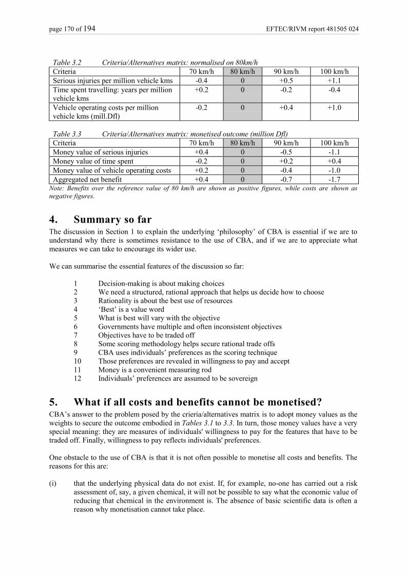
page 170 of 194 EFTEC/RIVM report 481505 024
Table 3.2 Criteria/Alternatives matrix: normalised on 80km/hCriteria 70 km/h 80 km/h 90 km/h 100 km/hSerious injuries per million vehicle kms -0.4 0 +0.5 +1.1Time spent travelling: years per millionvehicle kms
+0.2 0 -0.2 -0.4
Vehicle operating costs per millionvehicle kms (mill.Dfl)
-0.2 0 +0.4 +1.0
Table 3.3 Criteria/Alternatives matrix: monetised outcome (million Dfl)Criteria 70 km/h 80 km/h 90 km/h 100 km/hMoney value of serious injuries +0.4 0 -0.5 -1.1Money value of time spent -0.2 0 +0.2 +0.4Money value of vehicle operating costs +0.2 0 -0.4 -1.0Aggregated net benefit +0.4 0 -0.7 -1.7
Note: Benefits over the reference value of 80 km/h are shown as positive figures, while costs are shown asnegative figures.
4. Summary so farThe discussion in Section 1 to explain the underlying ‘philosophy’ of CBA is essential if we are tounderstand why there is sometimes resistance to the use of CBA, and if we are to appreciate whatmeasures we can take to encourage its wider use.
We can summarise the essential features of the discussion so far:
1 Decision-making is about making choices2 We need a structured, rational approach that helps us decide how to choose3 Rationality is about the best use of resources4 ‘Best’ is a value word5 What is best will vary with the objective6 Governments have multiple and often inconsistent objectives7 Objectives have to be traded off8 Some scoring methodology helps secure rational trade offs9 CBA uses individuals’ preferences as the scoring technique10 Those preferences are revealed in willingness to pay and accept11 Money is a convenient measuring rod12 Individuals’ preferences are assumed to be sovereign
5. What if all costs and benefits cannot be monetised?CBA’s answer to the problem posed by the crieria/alternatives matrix is to adopt money values as theweights to secure the outcome embodied in Tables 3.1 to 3.3. In turn, those money values have a veryspecial meaning: they are measures of individuals' willingness to pay for the features that have to betraded off. Finally, willingness to pay reflects individuals' preferences.
One obstacle to the use of CBA is that it is not often possible to monetise all costs and benefits. Thereasons for this are:
(i) that the underlying physical data do not exist. If, for example, no-one has carried out a riskassessment of, say, a given chemical, it will not be possible to say what the economic value ofreducing that chemical in the environment is. The absence of basic scientific data is often areason why monetisation cannot take place.

EFTEC/RIVM report 481505 024 page 171 of 194
171
(ii) The underlying physical data may exist but not be in a form suitable for monetisation. Recallthat the money values reflect preferences. Now suppose the physical data take the form of ‘areduction of X tonnes in biochemical oxygen demand (BOD)’ in a river. Individuals do nothave measurable preferences for BOD. What they have preferences for is more or less waterquality. The ‘object’ of preferences does not correspond to the physical measure of theenvironmental change. This is the so-called correspondence problem.
(iii) The relevant physical data may exist and may correspond to what people value, but theresearch may simply not have been done. Consider biological diversity. There are numerousstudies of the willingness to pay to conserve biological resources (e.g. endangered species)but hardly any that tells us what people's preferences are for diversity per se.
Note that we have not listed the ‘impossibility’ of monetisation as one of the reasons whymonetisation may not exist. This is because, in principle, people have preferences for all the changesthat are likely to take place in the context of policies and projects. But there will be problems if thereare difficulties of perceiving the relevant change. This may be the case with very small risks, forexample, or with very small changes in something like river flow.
What should be done if some costs and/or benefits cannot be monetised?
Depending on the context, it may still be possible to reach a conclusion about the outcome of theCBA. Consider the matrix below:
Bnm > 0 Bnm < 0 � Cnm > 0Bm > Cm Accept ?Bm < Cm ? Reject
Bm refers to monetised benefits and Bnm refers to non-monetised benefits. Similarly with costs, C.
Suppose monetised benefits exceed monetised costs and that Bnm > 0. Then the project or policyshould be accepted even though we do not know the size of non-monetary benefits because the non-monetary benefits will simply be additional to the monetised benefits which in turn already justify theproject.
If, on the other hand, Bm > Cm but Bnm is negative, i.e. there are non-monetised costs, we will notknow whether to accept or reject the project/policy. But we can ‘invert’ the analysis and ask whether,judgementally, we think the net Bm (Bm-Cm) is sufficient to compensate for the non-monetary costs.At the very least, the procedure forces the decision-maker to list costs and benefits and to asksearching questions about the non-monetised costs.
The same procedure can be followed for the final row of the matrix.
What should be avoided is the view that if we cannot monetise everything, nothing should bemonetised. This view amounts to rejecting valuable information about people's preferences.Moreover, as we see later, rejecting monetisation simply raises all kinds of other problems.
6. The issue of geographical boundsOne issue highlighted by the steering group for this paper is the geographical bounds of CBA. It isusual to set the nation as the geographical boundary, so that any costs and benefits that accrue outsidethe nation do not ‘count’ in the CBA. But the principles of CBA do not in fact favour this popularrule, for CBA is indifferent to whom the beneficiaries and losers are. National boundaries areessentially political constructs, whereas benefits and costs relate to anyone securing a welfare gain orloss.
page 172 of 194 EFTEC/RIVM report 481505 024
There are in fact some good reasons for keeping the nation as the 'working rule' for the geographicalbound of CBA but relaxing that working rule in certain contexts.
First, where the issue in question relates to impacts which are the subject of a binding (voluntary orlegal) agreement internationally, then the relevant costs and benefits should be defined in terms of thesignatories to that agreement. In the context of global warming or stratospheric ozone depletion, forexample, the relevant benefits and costs would be global. If the Netherlands was deciding on itsclimate policies then it would be proper that any costs incurred by other countries because of Dutchpolicy should be presented as negative benefits of the policy. The benefits to other countries ofreducing greenhouse gases in the Netherlands should similarly be included in the benefit estimates.While there may be circumstances where the CBA might be defined in terms of national gains andlosses, the fact of signing an international agreement is an acknowledgement that others' gains andlosses are just as relevant as domestic gains and losses.
Second, the same principle applies where the agreement is international but not global. Acid rainwould be an example. The damages due to the emissions from the Netherlands that are relevant arethose to the entire UNECE region because the Netherlands is a signatory to the Long-RangeTransboundary Air Pollution Convention.
Third, some objects of policy may not be the subject of national property rights only. A cultural assetthat is a World Heritage Site, for example, is, effectively, an asset over which the world as a wholehas property rights in some form. It is then wholly appropriate to measure the benefits of conservingthat site so as to include the benefits to people outside national boundaries.
Fourth, even without international legal agreements, any nation may feel a moral obligation toaccount for its impacts on others.
What should be done when there is no moral obligation and no legal agreement but transboundarybenefits and costs occur anyway? There is a probable asymmetry here. For costs it is easy to see thatthere may still be a case for counting them in to the CBA. The reason for this might be a moralobligation (above) but it may also be self-interest: neglect of the costs to others now might invitesimilar neglect of costs imposed by another country on the Netherlands in the future. Simple self-interest dictates the ‘good deed’ approach. It is less obvious when it comes to transboundary benefits.The argument could be that it is best to include them on the grounds that this would encourage othersto do likewise for reciprocal projects and policies, encouraging them to increase the size of suchbeneficial projects and policies. But there may be taxpayer resentment at the idea that nationaltaxpayers are paying from non-nationals to gain from a project. The issue could be resolved, ofcourse, if such transboundary benefits could be appropriated by pricing policies, i.e. charging others.
Overall, the geographical bounds issue is one that has probably not been treated in a very logicalmanner in CBA in the past. We have suggested some rules to deal with the different contexts in whichthis issue might arise.
7. Experience with CBACBA is quite widely used in some countries and hardly at all in others. Does individual countryexperience explain how to get CBA accepted for decision-making? It certainly helps to explain why itsecures greater acceptability in some contexts rather than others.
There are two main contexts for monetisation of expressing costs and benefits in monetary terms:regulation and liability. There are other contexts, such as green national accounting anddemonstrating priorities for policy, but the history of monetisation is, by and large, a history ofregulation and liability. In the regulation context, it is CBA that is relevant. In the liability context,only damages are relevant so money values of damages are the relevant measure, not CBA.

EFTEC/RIVM report 481505 024 page 173 of 194
173
RegulationThe regulatory role of CBA is most advanced in the USA. The major piece of legislation in thisrespect was Executive Order 12291 (1981) which required a benefit-cost assessment of newregulations which impose significant costs or economic impacts. EO 12991 required that, for any newregulation, ‘the potential benefits outweigh the costs’ and that ‘of all the alternative approaches to thegiven regulatory objective, the proposed action will maximise net benefits to society’. EO 12291helped to engrain cost-benefit thinking in federal agencies, although actual cost-benefit studies wereapplied in a non-uniform manner across agencies. The US Environmental Protection Agency was oneof the agencies to take the requirement to carry out cost-benefit studies most seriously. But therequirements for using CBA vary across statutes.
Several court cases have established that CBA cannot be used by agencies unless explicitly authorisedby statute. However, even where analysis of costs and benefits was not explicitly required, the USEPA tended to adopt regulations on the basis of CBA studies. Thus, compared to Europe, CBA is farmore influential in the USA than a simple comparison of formal requirements would suggest.
Whether CBA is actually used more than the statutes require, it remains the case that US legislatorsquite clearly regard CBA as not being relevant in a number of regulatory contexts. It is tempting tothink that this has something to do with doubts about the credibility of benefit estimates, but it issignificant that, while the costs of regulation are given more consideration than the benefits, severalstatutes and corresponding court cases specifically exclude even the costs from consideration instandard setting. This suggests that EO12991 was never consistent with the philosophy underlyingmuch of the environmental legislation. Nonetheless, new regulations require the approval of theOffice of Manpower and Budget (OMB) and OMB could therefore enforce EO12991 over and aboveactual statute requirements.
EO 12991 was superseded by EO 12866 in 1993. This replaced the ‘benefits outweigh costs’provision with ‘benefits justify costs’. Benefits include ‘economic, environmental, public health andsafety, other advantages, distributive impacts and equity’ and may not all be quantified. In effectthere was no formal requirement that benefits actually exceed costs in a quantitative sense. Somecommentators suggest that EO 12866 endorses CBA as an ‘accounting framework’ rather than an‘optimising tool’.
The situation with respect to CBA in the USA is therefore an uneasy one, but, in so far as theExecutive Orders can be used to ‘impose’ CBA, CBA remains very influential in the US system. Thata number of the statutes to which the EOs might apply explicitly exclude CBA considerations, andeven cost considerations, suggests, however, that alternative philosophies are still important.Morgenstern (1996)22 suggests that the whole culture of EPA is rooted in legal and scientificobjectives, and some of the 1970s ideology about the ‘environmental cause’. As such, economicconsiderations were always likely to be secondary. Moreover, economists are very much in theminority at EPA, and the educational background of most of the employees is such as to reinforce theview that economic analysis is a secondary consideration in environmental protection. Morgenstern(1996) suggests two further reasons for the ‘downgrading’ of economic influence in US regulation.First, there has been the rise of a ‘win win’ philosophy which suggests that environmental protectioncan be secured at no discernible economic cost. We noted earlier that this is an illusory approach todecision-making. Secondly, ‘spin’ and ‘PR’ have tended to replace awkward decision-making. This,we might observe, is not a trend confined to the USA.
In the European context, CBA has secured an increasing role in decision-making. Article 130r(3) ofthe Treaty of European Union (the Maastricht Treaty) requires action to take into account severalfactors of which one is ‘the potential benefits and costs of action or lack of action’. Clearly, some 22 Morgenstern, R. (1996) Economic Analyses at EPA: Assessing Regulatory Impact, Washington DC:Resources for the Future.

page 174 of 194 EFTEC/RIVM report 481505 024
form of CBA is mandated by this provision. Up to about 1990 EU environmental policy was, by andlarge, effected with little formal evaluation of policy taking place. In some cases, virtually noassessment of benefits and costs was undertaken, even at the qualitative level. This appears to be thecase even for major and expensive Directives such as the Wastewater Directive, Drinking WaterDirective, Habitats Directive and the Bathing Waters Directive.
Some sort of formal appraisal was undertaken on water pollution and on the impacts of the SingleMarket before 1990. The number of studies indicated is deceptive, however, since they are oftenstudies repeated for separate countries, or, in the case of water pollution, for different substances.Nonetheless, the fact that impacts were measured for individual Member States is an indicator of theimportance of the issue. The multiplicity of studies on water tends to reflect the significant number ofkey pollutants involved in water pollution. The other major targeted area for simulations of costs andeffectiveness was the carbon-energy tax. In turn, this proposed Directive attracted probably the singlelargest opposing lobby of any Commission proposal, so that the studies are a natural outcome,anticipated or ex post, of that process. Studies of Directives per se remain very few and these tend tobe concentrated into the period since 1994.
Within individual European member States, CBA has varying degrees of influence. In the UK, forexample, it has effectively become embodied in ‘regulatory impact assessments’ (RIAs), although thequality of those assessments varies substantially. In Norway, monetised health damages have beenused extensively to guide policy on air pollution control.
Liability and damagesThe second major area for the use of monetised estimates of environmental damage has been in thecontext of liability. In the USA this has related mainly to contaminated land and oil spills. Outside ofthe USA, however, there is little experience of this context for monetisation. This reflects the fact thatliability legislation is less extensive, although there are examples of monetised damages being used incases of oil spills. Additionally, damage estimates have been used in some quasi-judicial contextssuch as the licensing of abstractions from rivers in the UK.
Factors explaining different uses of monetisationWhat can be learned from the regulatory and liability contexts for monetisation? The essential lessonsappear to be as follows:
(a) Where there is a strong tradition of ‘efficiency in government’, as in the USA where the traditiondates back to the pre-war era, there is likely to be a greater use of CBA.
(b) Efficiency in government as a philosophy is partly a political and cultural issue. Political partiesstrongly dedicated to free market principles and concerns for the ‘rights’ of taxpayers are perhapsmore likely to believe in CBA in the belief that it will limit, rather than enhance, regulation. Thefact that CBA often shows environmental regulation to be strongly beneficial may perhapsaccount for some of the retreat from CBA in the USA where free market principles are strong. Inother words, CBA may not have had the result the free marketers thought it would have. On theother hand, CBA can, in some contexts, slow down the regulatory process by adding to theburdens of the regulatory agency.
(c) The USA has very strong lobbying groups in favour of CBA. In turn those lobbying groups maythemselves have free market principles which produce an anti-regulation philosophy. An examplewould be the American Enterprise Institute, which is a free-market organisation that produceshigh quality critiques of government policy.
(d) As opposed to lobbying, the US is strong on policy analysis institutes, ‘think tanks’ that have theexplicit purpose of monitoring and appraising government policy. It is much harder to identifycomparable policy analysis institutes in Europe. Those that exist do not produce research of thequality of, say, Resources for the Future, of the World Resources Institute. This means that, unlike

EFTEC/RIVM report 481505 024 page 175 of 194
175
the USA, those within governments in Europe have few external alliances that they can make tofurther RDM.
(e) There is a strong tradition in some countries of secondment of academics to government, or closelinks between academia and government. The Central Bureau of Statistics in Norway producesnot only statistical and other support services for government but is an acknowledged source ofstrong economic research. In the USA, staff at policy analysis institutes are regularly seconded togovernment. Europe has perhaps less of a tradition in this respect, although Italy is notable for therole that academics have played in formulating government environmental policy.
(f) Liability legislation is a powerful impetus to the use of monetisation. One way or the other,damages must be estimated and once liability extends to environmental damage it is difficult tosee what criteria could be used for assessing damages other than monetisation methodologies ofthe kind used in environmental economics. The other feature of liability is that it forcesmonetisation 'into court' so that monetary estimates of damage have to be credible because theywill be debated and disputed by differing experts.
Clearly, then, some legal or quasi-legal requirement that costs and benefits be considered in (a)regulation and (b) damage liability could open the way for wider and better use of CBA in Europe.The issue becomes one of how to persuade the decision-makers that this would be a sensible thing todo. The lessons from history are essentially that the most powerful argument in favour of doing this isthat CBA encourages the search for more efficient regulation and that it is a useful barrier to over-regulation.
8. Obstacles to the use of Cost-Benefit AnalysisThe philosophy of CBA gives clues to why it is sometimes difficult to secure adoption of CBA inpractice. We classify the obstacles as issues of philosophy and content, and as issues of process.
Philosophy and content
1 Credibility – CBA is a quantitative technique and the resulting quantities are oftenuncertain. Decision-makers will generally be averse to uncertainty.
2 Morality – CBA uses money values and there is often a ‘moral’ hostility to usingmoney as the measuring rod.
3 The efficiency focus– CBA has economic efficiency as its goal. But governmentshave multiple objectives, hence CBA appears to be partial and non-comprehensive.
4 The democratic principle – while it may seem odd to suggest that decision-makersoppose ‘democracy’, there are concerns about the legitimacy of reflecting preferencesin all contexts.
page 176 of 194 EFTEC/RIVM report 481505 024
Process
5 Flexibility – some decision-makers may feel that CBA compromises their flexibilityof decision-making.
6 Participation – CBA is sometimes criticised for being non-participatory.
7 Capacity – CBA requires a certain level of expertise on the part of those using it orjudging its results.
We address each of these issues in turn, and in doing so, suggest ways in which the obstacles may bereduced. Before doing that, we need to address a very important issue that is rarely addressed indebates about the ‘proper’ way to make decisions. This is the baseline issue. This issue concerns whatwe would do if we did not adopt CBA as the general basis for making decisions.
9. BaselineCBA is a coherent decision-making guide based on the concept of economic efficiency, as notedabove. But it is only one such guide. If decisions are not made with the help of CBA then they musteither be made on an ad hoc basis, i.e. with no particular systematic guidance, or using some otherguidance procedure. On the assumption that purely ad hoc decision-making is rejected on thegrounds that it is not rational, the alternatives to CBA are the other systematic procedures that mightbe used. While this may seem obvious, one of the curious features of the debate about CBA is that itis often presented as if the alternatives to CBA are somehow free of the criticisms that are advancedagainst CBA. This is the ‘baseline’ issue. If CBA is challenged, it is logically proper that the criticoffers an alternative procedure which is ‘better’.
The very first test of the alternative approach is to see if it is free from the criticisms that have beenadvanced against CBA. Establishing this rule is essential in the discourse about RDM.
Space forbids that we discuss the alternative procedures in any detail (see EFTEC, 2001)23. The main‘contenders’ for rational decision making are:
Environmental impact assessment (EIA)Life cycle analysis (LCA)Risk assessment (RA)Multi-criteria analysis (MCA)Cost effectiveness analysis (CEA)Cost-benefit analysis (CBA)
Table 9.1 below shows that techniques are often complementary. CBA cannot be carried out, forexample, in the absence of risk assessments of health impacts or of environmental impact assessmentin some form. Similarly, LCA can be combined with CBA to produce combined economic valuationand life cycle assessment. Similarly, LCA and EIA have close similarities if the EIA takes on acradle-to-grave impact stance. EIA is, of course, also essential for CBA: all valuation techniquesrequire the physical impact data to work with. Finally, even if techniques appear to be different, theymight profitably be combined. For example, a CBA might be combined with some scoring andweighting procedures (MCA) for those impacts that are not readily monetised. The interconnectionsbetween the techniques indicate that a debate about which technique is better can easily bemisleading. The techniques tend to build on each other. Nonetheless, we can try to see whether often
23 EFTEC (2001), Guidance on Using Stated Preference Techniques for the Valuation of Non-Market Effects,report for the UK Department of the Environment, Transport and the Regions, London (summary guidancereport forthcoming at www.detr.gov.uk).

EFTEC/RIVM report 481505 024 page 177 of 194
177
quoted criticisms of CBA are avoided by adopting one of the other techniques. Annex 1 lists eachprocedure and highlights the main features and the advantages and disadvantages of each one.
The overview in Annex 1 serves to reveal a number of important observations about so-calleddecision rules.
First, only two appraisal techniques actually provide a decision rule. A decision rule is one thatindicates whether the policy or project is potentially ‘good’ or ‘bad’. Decision rules embody tests todetermine this. CBA has such a test, namely that benefits exceed costs. No other appraisal techniqueembodies this test. Comparative Risk Assessment (see Annex 1) comes close because it has a rule thatsays the choice should be that option which has the highest risk reduction per Dfl expended. But it islimited to this context. Nor does it say whether any risk reduction option should be accepted, i.e. itanswers the question A or B? but does not answer the question: A or B or neither?
Table 9.1 Relationships between evaluation techniquesLCA RA MCA CBA
EIA EIA can be doneon the basis oflife cycleimpacts. Usuallynot done.
RA could be aninput to EIAprovided EIAdeals withpotentialdamages, not justemissions.
EIA needed toprovide theimpact data forthe MCA.Environmentalimpacts would beone 'goal'.
EIA essential as aninput to CBA.
LCA XXXXXXXX Risks could beevaluated on alife cycle basis.Generally notdone.
MCA could takelife cycle impactsas one goal.
LCA consistent withthe 'with andwithout' principle ofCBA.
RA XXXXXXXX XXXXXXXX RA essential asinput to MCA.
RA is an essentialinput to CBA, e.g.premature mortality,morbidity etc.
Second, decision-makers may not want an explicit decision rule. As discussed later, they may prefer adecision technique which leaves them flexibility of choice. Several rules provide this flexibility, e.g.MCA, CEA. CBA and CRA, on the other hand, present the result in terms of a ‘cut and dried’ rule.
Third, and contrary to the way in which they are often discussed, some of the techniques are onlyinputs to decision-making. They do not provide guidance on how to make decisions. LCA and EIAfall into this category. LCA is often presented as if it provides a decision-making rule, but it onlybegins to do this if the life cycle inventory is weighted by factors reflecting the importance of theimpacts. Some LCA does this, but procedures for selecting weights are often arbitrary, i.e. have nounderlying theoretical rationale. Where the weights have a rationale, as with monetary damageweights, LCA would effectively be equivalent to CBA if other costs and benefits are also taken intoaccount. Invariably they are not accounted for in LCA.
Fourth, few of the techniques explicitly address time. There are several ways in which time shouldenter an analysis. First, impacts are distributed over time and if the weighting procedure is preferencebased, future impacts should be ‘discounted’ to reflect the fact that individuals care less about thefuture than the present. The idea of discounting the future is thought by some to be inconsistent withthe objective of sustainability. This not necessarily true. Even governments tend to discount thefuture. What can be said is that techniques that fail to address the discounting issue (even if theyconclude that future impacts should not be discounted) must be at least non-comprehensive. Thesecond effect of time is that some impacts will become less or more important over time. This is

page 178 of 194 EFTEC/RIVM report 481505 024
different to discounting and simply refers to the fact that individuals’ intensity of preference forsomething may change, often with income. In CBA this issue is handled by a falling (rising) relativeprice. Other techniques appear not to address the issue at all. Note that CBA explicitly addresses bothtime-related issues24.
The failure to address the baseline issue in public debate is not confined to the comparison of CBAwith other techniques. It is just as common, for example, in discussions about market-basedinstruments such as environmental taxes. Taxes, it is often said, will harm the poor and do damage toa nation’s competitiveness. Apart from the fact that these statements are usually made withoutsupporting evidence, the fact is that the same criteria are not used with respect to the alternative formof regulation. Thus, it may well be the case that traditional regulation does more damage tocompetitiveness and to low income groups than the tax option. Instead, the arguments tend to bepresented as if the alternative to taxation is no regulation at all. The phenomenon is common inpolitics generally (e.g. ‘single issue’ pressure groups).
How might the baseline syndrome be overcome? For advocates of any one procedure (e.g. CBA), itis important that they have a list of criteria by which the efficacy of a policy measure might bedetermined. These are not likely to be controversial (e.g. efficiency, equity, sustainability, impairmentof competition etc.). The controversy arises because interest groups select only one or two of thecriteria and argue about these, effectively giving the others no weight at all. Thus, an advocate of CBAshould first list the criteria, perhaps using policy statements already made, and should then ask thequestion: how would the alternatives to CBA compare against these criteria? Interest groups seekingto confine the debate to one or two criteria only should be asked why they ignore the other criteria andto place themselves in the position of a decision-maker who has to listen to, and account for, differentinterests and stakeholders. The criteria/alternatives matrix is a good way of organising this debate.
Determining the baseline is absolutely critical to policy debate. All too often, debate takes place as ifthe alternative to any given policy guidance procedure is to do nothing, to muddle through or to use adhoc procedures. In other debates, criticisms of one procedure, usually CBA, are stated withoutrecognition that the same criticisms often apply to the alternative procedure, and without recognitionof the fact that other procedures have other problems or that they are incomplete decision guidingprocedures. This section suggests that the use of matrix approaches can help different stakeholders seethe problem through the eyes of other stakeholders. At the very least, the matrix lays down the basisfor rational debate.
10. Obstacles: credibilityOne of the criticisms advanced against CBA is that the answers are not credible. Credibility rests onseveral factors: whether the final estimate of net benefits has ‘too wide’ a range; whether theassumptions made in order to achieve the estimates of net benefits are themselves credible; andwhether the estimates have been truly tested for their validity.
All are valid sources of concern in decision-making. The range of estimates tends to represent theunderlying uncertainty of socio-economic data. Social science data are not like ‘physical’ data.While both are subject to uncertainty, social science data are far more probabilistic since they reflectthe behaviour of millions of individuals. Thus uncertainty is endemic to social science. In terms ofchoosing between decision-making guidance, however, uncertainty per se is not the issue. Whatmatters is whether any one form of guidance is more uncertain than the others. Annex 1 shows thatmost guidance procedures are incomplete in that they do not account for all the information that onewould expect to be included in a rational decision. Thus, LCA and EIA make no reference to the costsof policies or projects, yet no rational decision can be made independently of costs for the reasonsraised in Section 1 above. Hence, even if CBA is more uncertain than other techniques (an assumption 24 But the state of play with respect to how these issues are addressed is not satisfactory. There is no consensuson appropriate discount rates nor is there much evidence on the correct rate at which relative prices change.

EFTEC/RIVM report 481505 024 page 179 of 194
179
that needs to be tested), it does not follow that some alternative technique is better. The greateruncertainty of CBA is simply being exchanged for a somewhat illusory certainty, illusory because it isachieved by simply ignoring other factors that should bear on how to make decisions. Consider CBA‘versus’ risk assessment. CBA may appear to be more uncertain than Risk Assessment because themoney values appear to add to the variables that are uncertain. Risk Assessment avoids monetaryassessment and hence reduces the level of uncertainty. But it does so by sacrificing a basicrequirement of decision-rules, namely telling us whether something is good or bad, desirable orundesirable. In effect, with Risk Assessment we have no idea whether any decision is ‘correct’because we have no absolute standard against which good or bad is measured. Risk Assessment doestell us that policy A is to be preferred to policy B if A secures more risk reduction per Dfl expendedcompared to B. But it does not tell us that A is itself desirable. Hence a whole different layer ofuncertainty is introduced with Risk Assessment.
The first rule for dealing with the ‘uncertainty means non-credibility’ argument is therefore to raisethe baseline issue again. What are the sources of uncertainty for each procedure? If CBA has one ormore sources of uncertainty, are these sources absent in the alternative procedures? What other formsof uncertainty do the alternative procedures have? Sometimes this procedure is known as ‘the bestgame in town’ argument: all approaches are imperfect – the issue is one of choosing the leastimperfect.
But CBA may have some special sources of uncertainty. First, it assumes that individualsthemselves behave rationally25. The rationality assumptions underlying CBA are quite strict. Forexample, it is assumed that individuals are capable of consistent preferences across a wide range ofgoods and services, including non-marketed environmental goods. Psychologists suggest thatindividuals may not in fact behave this way. They may, for example, break rules of ‘transitivity’,effectively preferring A to B, B to C but C to A. In other respects they may ‘trade’ between optionswithin a given ‘mental account’ but not between mental accounts. A mental account might be, say,the weekly shopping budget, while housing expenditures are in another account, and entertainment inyet another. They may have rational preferences within any account but not be willing to tradebetween, say, housing and shopping. Intransivity and mental accounts both create problems for theassumption that people have clearly defined preferences across all goods and services. Again, it isimportant to apply the baseline test. Are these problems avoided by adopting a different procedure?The answer is that, as long as the procedure is rooted in the idea that people’s preferences ‘shouldcount’, these problems are not avoided. They are, of course, avoided if people’s preferences arerejected as the basis for decision-guidance. Indeed, it could be argued that the fact of imperfectrationality is a ground for rejecting individual preferences. As noted in Section 1, ultimately, differentvalue systems cannot be avoided, but it was suggested there that the overthrow of individualpreferences is something that should be avoided unless absolutely necessary.
A second source of uncertainty of relevance to CBA is that pertaining to stated preferencetechniques26. A stated preference technique is based on a questionnaire of a random sample of thepopulation. Individuals are asked about their attitudes generally, about their attitudes to the specificgood, and about their socio-economic status. In choice modelling procedures they are also asked torank or rate a given package of attributes that together make up a project or policy, relative to someother package. They are not asked their explicit willingness to pay, but a price or cost of some sort isincluded as an attribute in the packages27. The analyst then infers the WTP from the answers provided.In contingent valuation the respondent is asked directly for his/her WTP, sometimes in response to
25 More strictly, that they behave rationally as a group, i.e. ‘on average’.26 EFTEC (2001), Guidance on Using Stated Preference Techniques for the Valuation of Non-Market Effects,report for the UK Department of the Environment, Transport and the Regions, London (summary guidancereport forthcoming at www.detr.gov.uk).27 Terminology varies, but choice modelling techniques include choice experiments, contingent ranking,contingent rating and pairwise comparisons. These are sometimes referred to as conjoint analysis. Note that notall variationsof choice modelling are equally robust.

page 180 of 194 EFTEC/RIVM report 481505 024
an open-ended question (what is your maximum WTP?) and sometimes in response to a close-endedquestion (are you willing to pay DflX?)28. These approaches, which are increasingly used in cost-benefit studies, are thought by some to add to the uncertainty in CBA. The reason for this is that thequestionnaires are hypothetical and hence the answers are hypothetical. The hypothetical nature of thequestionnaire is not itself a criticism. After all, the reason hypothetical questions are being asked isinvariably because there are no ‘real’ markets for the analyst to refer to. If the real markets existed, wewould not need to ask hypothetical questions. Nonetheless the answers could be biased (upwards ordownwards, but more usually it is thought the bias is upwards). The issue becomes one of finding outhow likely it is that the hypothetical answers diverge from the respondents’ ‘true’ WTP. To this end,stated preference techniques adopt many tests of validity. A well-designed and implementedquestionnaire should therefore minimise the biases. An example would be to conduct a statedpreference study at the same time as one using some other technique. An example might be a hedonicprice study whereby the influence of the environmental change in question on some market price (e.g.house prices) is determined. The WTP ‘revealed’ through the hedonic technique can then becompared with the WTP derived from the stated preference technique. But bias is likely to remain.This may not matter too much if there is some idea of the direction of bias and its probable scale.Research suggests that there is an upward bias in WTP responses, but it is not easy to say what thescale of this bias is.
While critics of stated preference techniques are often unaware of the tests embodied in a good study,the feeling that answers are not reliable indicators of true preferences remains. Since stated preferenceanalysis is an ongoing activity, and a great deal more research needs to be done, it may be that futureresearch will resolve the issue of how large the hypothetical bias is. Accepting that, for the momentanyway, we do not know, the same baseline issue arises. If we adopted any other technique, would weavoid the supposed additional bias in stated preference answers? One view suggests that we would notavoid this bias because it is a feature of the hypothetical nature of the questionnaire. The bias wouldtherefore also be present in any technique that requires the views of potential beneficiaries and losersto be determined. On another view, it is the very fact that money is involved that produces the bias, orat least part of it. If so, perhaps choice modelling techniques where money is not explicitly mentionedwould avoid the problem. At the moment, we do not know if this is the case because so few choicemodelling experiments exist (outside of the transport field anyway).
Ultimately, then, the issue of uncertainty reduces to:
(a) determining whether it is any better or worse if some other technique is used; and(b) the view taken about the ‘special’ bias that may reside in the use of stated preference techniques.
Note, of course, that most cost-benefit studies still do not make use of stated preferencetechniques so that, even if it is felt there is some special bias, this does not mean that most CBA isbiased.
11. Obstacles: moral objections to Cost-Benefit Analysis andthe issue of democracy
Some critics of economic valuation and CBA find its emphasis on opportunity cost morallyobjectionable. It is often argued, especially in the health care context, but also in safety andenvironmental contexts, that certain outcomes of policies should not be subject to budgetconsiderations. Patients, it is said, should be treated with the best health care available regardless ofcost; road and rail safety should be an absolute priority regardless of cost; and environmentalprotection is an absolute moral imperative and cannot be subject to rationing by cost. The maindifficulty with these views is that they ignore the meaning of cost. As Section 1 noted, the propermeasure of cost is the benefit that is forgone by allocating expenditure to a chosen project or policy.If money is spent on A it cannot be spent on B. While A may have some of the characteristics of
28 Close ended question formats take the form of bidding games, dichotomous choice and payment ladders.

EFTEC/RIVM report 481505 024 page 181 of 194
181
being ‘moral goods’, like health and safety, so might B. Money spent on road safety cannot be spenton cancer research or hospice care. The principle can be extended. If funds are raised to finance arisk reducing expenditure, the effect may be to impose risks on the people who are taxed to raise thefunds29. The essential point is that cost is not ‘just money’: it is an expression of resources that couldbe used for all kinds of other, perhaps equally deserving, purposes.
More fundamentally, some critics object that, by focusing on the preferences of individuals, economicevaluation takes account only of self-interest. If an individual has a preference for or againstsomething, it might appear that the preference will be formed on the basis of what that individualjudges to be best for himself. A short way of expressing this point is to say that the individual acts outof self-interest. Indeed, this is how ‘consumer sovereignty’ or ‘economic rationality’ is oftencharacterised. But the issues for which monetary valuation will be used will often be those where thepublic interest is the issue, i.e. what is best for society as a whole.
Whether or not the public interest is the same thing as the sum of individuals’ self-interests is acontroversial question in political philosophy. So too is the question of whether it is better if, whenacting in the political arena, individuals act in pursuit of their private interests, constrained only byrules of procedural fairness, or if they act on the basis of ‘public spirited’ or ‘citizens’ preferences.Viewed in some philosophical perspectives, it is wrong to reach collective decisions by adding upself-interested preferences. The proper procedure is to ensure that the context of decision-making isone where citizens’ preferences are expressed. That context would appear to be the political arena,not the outcome of a context where, say, experts collect questionnaires from respondents who areasked for their stated preferences30. (We say ‘appear’ because, it is far from clear that preferencesrevealed in the political process are less self-interested and more public-spirited than those revealedby the same people in the market.)
As a first response to this criticism, we emphasise that CBA is not a substitute for the politicalprocess; it merely provides information to the actors in that process. Someone who believes that aparticular policy is morally required, or is morally prohibited, can properly try to persuade otherpolitical actors to share this belief and to act on it, whatever the results of a CBA. For example, ifsomeone believes that everyone has a moral obligation to accept a certain increase in taxation in orderto pay for a programme to conserve endangered species, the fact that the programme fails to satisfythe CBA test does not require them to change their belief: they are entitled to conclude that otherpeople are evading their moral obligations. But the CBA results remain meaningful information aboutwhat people really are willing to pay for the programme.
However, it is a mistake to think that CBA takes account only of self-interested preferences. It takesaccount of whatever preferences people have, for whatever reasons they have them. For example, aperson may want an environmental asset to continue in existence even though he makes no direct useof it, nor intends ever to make any use of it. To the extent that he is willing to forgo other things thathe values in order to conserve the asset, he has a preference for its conservation and its conservation isa benefit to him. He might be motivated by fact that without the asset’s continued existence, he couldnot enjoy it vicariously through television or film. This motive might be described as self-interested.But he might also be motivated simply by wanting the asset to continue in existence for its own sake,or because he sees himself as a ‘steward’ of the environment, or because he wants it for his childrenor future generations to enjoy. In short, there is nothing in the concept of preference that tells us thatpreferences have to be motivated by self-interest.
Overall, then, those who hold moral views about CBA may well be objecting to the underlyingutilitarian philosophy of CBA. But they may also share some confusions about the nature of economic
29 This aspect is explored in the literature on ‘risk-risk’ analysis. See W K Viscusi (1998) Rational Risk Policy,Oxford: the Clarendon Press.30 This is the view taken, for example, by Mark Sagoff. See M Sagoff (1988), The Economy of the Earth:Philosophy, Law and the Environment, Cambridge: Cambridge University Press.

page 182 of 194 EFTEC/RIVM report 481505 024
valuation and the fundamental role played by the concept of opportunity cost. How might theseconfusions be reduced? Again, there is no substitute for reasoned discourse. The CBA advocateshould always be sure that those objecting to it are asked whether the moral implications of theirviews have been fully worked out, by seeking to explore the cost of those views and the implicationsof ignoring that cost. Moral objectors may then still have a residual objection to CBA based on theview that balancing gains and losses ignores the ‘absolute rightness’ of avoiding a particular form ofloss. The political process, if fairly formulated, is then the right place to debate those claims. What isnot justified is excluding consideration of costs and benefits from that process.
12. Obstacles: the efficiency focus of Cost-Benefit AnalysisSection 1 noted that governments have multiple objectives and those objectives often conflict. Oneprocedure for ‘trading off’ objectives is multi-criteria analysis (MCA). MCA does not require themonetisation of objectives but it does require a rational analysis of what has to be surrendered forwhat. MCA is discussed further in Annex 1. The important feature of MCA is that it embracesobjectives that CBA appears not to embrace. For example, it could include a distributional objective(fairness, equity), some assessment of sustainability, and wider national concerns such ascompetitiveness, employment, regional balance etc. The matrices introduced in Section 2 were in factthe kind of matrix with which MCA would begin. The advantage of these matrices is that decision-makers are forced to set out the criteria by which policy might be judged, and they are forced toquantify the effects of policy choices. Some policy analysts draw attention to another importantfeature of such matrices: they make it clear to everyone else, the public included, what the analyticalreasoning is behind potential decisions31. This encourages openness and appreciation that disciplinesother than economics have valuable inputs to make.
If MCA is ‘wider’ than CBA why not recommend MCA rather than CBA? The question is somewhatmisleading because CBA is in fact a particular form of MCA. There is nothing in MCA that saysefficiency is not important and nothing that says impacts should not be monetised where appropriate.If there is an ‘equity’ goal this may not be suited to monetisation, in which case something that ismore efficient but less equitable must be traded against something that is less efficient and moreequitable. The efficiency status cannot be determined, however, without some form of CBA32. ThusCBA can, and should, be an input into MCA.
Proceeding to MCA without CBA can also be dangerous. Some of the problems are:
(i) Many MCAs do not account for public preferences at all, but use expert judgement. This runscounter to the ‘democratic’ principle already introduced;
(ii) MCAs face considerable difficulties with time (discounting and changes in relative values);and
(iii) MCAs often risk double counting of objectives.
Provided great care is taken over the preparation of MCA, then, it is, as interpreted here, a wholly rationalway of presenting policy options. But it in no way precludes CBA which must be part of it.
31 This is stressed, for example, in D MacRae and D Whittington (1997), Expert Advice for Policy Choice,Georgetown University Press, Washington DC.32 CBA can in principle integrate equity and sustainability into its analysis. Few CBAs attempt to incorporatesustainability requirements, but integrating equity concerns was once very popular in CBA practice.

EFTEC/RIVM report 481505 024 page 183 of 194
183
13. Obstacles: flexibility of processAn important institutional factor that inhibits the use of CBA is the demand by policy makers forflexibility of choice. Imagine a technique, like CBA, say, that produced precise estimates of costs andbenefits such that the benefit-cost rule could be clearly and immediately identified. If CBA were theonly form of policy guidance, the policy-maker would merely have to assent to whatever the CBAresult produced. This limits the freedom of choice of the policy-maker and hence makes him or herresent techniques that appear to usurp that freedom. Decisions become ‘technical’ rather than a matterof judgement. The more quantitative the technique, and the more it embodies a decision rule in thesense advanced earlier, the less flexibility that approach will appear to afford the decision maker.
Flexibility is a legitimate concern, but it can be preserved whilst still employing CBA. No onetechnique should appear as providing the 'right' solution. It is an added piece of information which atleast orders the information available in some logical way. Thus, information on what the likelyimpacts are of a policy is the least that should be expected. How far quantification and aggregation ofthose impacts then take place depends on the context. But, there has to be some guidance. It is amatter of 'appraisal thinking' rather than the provision of exact numbers and outcomes. Again, thealternatives/criteria matrix helps because it places the CBA result in a wider context. The decision-maker is then free to introduce other criteria and to weight them accordingly.
The matrix/CBA approach is to be preferred to one alternative widely met in decision-makingcontexts. Many would argue that what matters most is how decisions are made. It may be that aprocedure using public participation is regarded as more important than one based on some balancingof costs and benefits. In some cases, the two may be combined, as with modern approaches toeconomic evaluation through the adoption of questionnaire-based approaches. Process is alsoimportant at the political level: consultation with parties who are, or represent in some way, thestakeholders offers some guarantee that the interlinkages referred to in previous chapters will becaptured. But process is not sufficient. Processes have to be informed by facts and by some orderingof the facts. Essentially, all the appraisal techniques reviewed in this chapter are about this process ofordering, of placing gains and losses into some framework so that they can be compared. Another wayof thinking about it is that process does not guarantee rationality of decisions. Equally, decisionscannot be made and cannot be effective without efficient process, not least because those excludedfrom the process may well 'block' a decision or at least make its implementation difficult.
14. Obstacles: is Cost-Benefit Analysis non-participatory?Modern approaches to project and policy appraisal rightly stress the need for public participation inthe process of appraisal. While participation is often seen as an end in itself, it is also a necessaryingredient for economic efficiency. The reason for this is that lack of participation can easilyengender opposition to a project or policy, making it difficult to implement and costly to reverse.Participation may also produce better policy and project design since those most affected are closer tothe issue than analysts and decision-makers. In the economic development literature, it is wellestablished that development projects are more likely to succeed if communities and gender groupsare involved in the process. Appraisal techniques are often criticised because they may omit thisparticipatory feature of decision-making. Stated preference techniques, however, have an importantrole to play in securing participation, a role that emanates directly from the fact that the techniqueselicit all kinds of information about attitudes, motivations, preferences and willingness to pay/acceptcompensation.
The literature is not always clear on the meaning of the term ‘participation’. At least three versions ofthe term appear: (a) participation as consultation, i.e. taking account of the preferences of affectedparties; (b) participation as influence, i.e. ensuring that affected parties influence the direction andform of the project or policy; and (c) participation as benefit-sharing, i.e. ensuring that affected partiesreceive a share of the resulting benefits. In any of these contexts great care needs to be taken that all

page 184 of 194 EFTEC/RIVM report 481505 024
genuine stakeholders are consulted. Stakeholders may include non-users, so that limiting the focus ofparticipatory processes to directly affected parties only can be inefficient. This reinforces the need toensure that proper sampling of opinion is undertaken. Simply working with a focus group of ahandful of people is unlikely to meet the requirement that a reasonable sample of opinion be surveyed.Even in the context of wider ‘community meetings’, participants may be far from being a randomsample. Meetings may be dominated by activists, by those who can afford the time to attend suchmeetings, and may be subject to strategic behaviour because of the potential for any one individualdeliberately to influence what others say. The more discursive approach to participation can, however,enhance the amount and perhaps the quality of information provided because responses tend to bemore open-ended and not restricted to the questions that the analyst tends to ask.
CBA can therefore be participatory if it makes used of stated preference techniques. Moreover, thereare good reasons to suppose that the rigorous statistical requirements for sampling will make a statedpreference approach more useful for participatory analysis than other, more conventional approachesto participation.
15. Obstacles: capacityA final obstacle to the use of CBA is the fact that, like all economic techniques, it requires an input oftime in order to understand the underlying rationale and some of the technical details. However welltrained decision-makers are, there will always be a residual element that does not invest time in tryingto appreciate the logic of CBA. Much the same goes for other guidance techniques and, for thatmatter, with scientific analysis generally. There are no easy cures here. Decision-makers are humanbeings, given to all the foibles, prejudices and irrationalities that make humans generally ratherinteresting. The matrix approach suggested in this paper would, however, help to expose those whowould want to reject rational criteria and who would refuse to measure gains and losses at all.
16. Getting Cost-Benefit Analysis into the process of decision-making
Clues about the ways in which CBA can be introduced to the decision-making process have been setout previously. They are gathered together in this section, together with several other observations.
First, there must be a rational discourse about decision-making in general. We suggested that thisshould be based on something like the alternatives-criteria matrix, which then forces the issue oftrade-offs to be recognised. Once this issue is understood, it is a small step to choosing between thevery limited number of RDM techniques that address the issue of weights and objectives in acomprehensive manner.
Second, CBA is unlikely to be brought into the process if it depends solely on the initiatives of groupswithin government. There must be external support in the forms of academic or research institutes, orNGOs, who favour the procedures. In turn, those institutes provide a forum for further debate, foradvancing the theory and practice of CBA, and they can act as peer reviewers and independentassessors. In short, there is a need for alliances between groups in government and groups outside,whilst at least some groups outside must retain their independence.
Third, there must be an ‘efficiency culture’ for CBA to thrive. If public spending is seen as more of amorally driven issue than one of efficiency, the chances that CBA will succeed are smaller. That said,it is incumbent on those who see spending as a moral issue to understand and account for opportunitycosts, i.e. for the moral consequences of inefficient spending.
Fourth, there needs to be some tradition of ‘senior ministries’ such that a ministry of finance isregarded as the ultimate guide on what is and what is not the proper subject of public expenditure. Inthe UK, no decisions about taxes or public expenditure can be made without Treasury approval. It is

EFTEC/RIVM report 481505 024 page 185 of 194
185
significant, then, that it is the Treasury that issues guidelines on how to appraise policies and projects,guidelines which broadly embrace the principles of CBA.
Fifth, CBA can appear as a dry, technical subject which deters close scrutiny and invites quickcriticism based on limited understanding. It is important that the subject be communicated in ascomprehensible manner as possible. Academics are not always keen to popularise their subject sincetheir own reward systems do not encourage this. Yet popularisation is important since that is the onlyway that the media will take an interest in the issue.
The suggestion in this paper is that CBA is best seen first as a way of thinking and organisinginformation; second as a significant part of an alternatives/criteria matrix approach to decision-making; and as a way of introducing a rational balancing of gains and losses in a world where trade-offs are the norm, not the exception. Thereafter it is an issue of forming alliances and arguing thecase.

page 186 of 194 EFTEC/RIVM report 481505 024

EFTEC/RIVM report 481505 024 page 187 of 194
187
Appendix A Types of formal appraisal procedures
Table A.1 Environmental impact assessment (EIA)Lists and measures in physical terms the various environmental impacts from a policy orproject.
Advantages Disadvantages
Forces systematic consideration of environmentalconsequences of actions, as input to decision-making process.Needed for techniques that do have a decisionrule.Points way to measures needed to mitigateserious negative impacts
Does not provide decision rule.Does not aggregate environmental impacts.Does not have conceptual link to non-environmental impacts.No obvious way of treating time dimension.
Table A.2 EIA plus scoring approachesLists and measures in physical terms the various environmental impacts from a policy orproject. Aggregates impacts using expert ‘scores’ and ‘weights’.
Advantages Disadvantages
Potential comprehensiveness high as any givenimpact can be included.Easy to use.
Weights and scores may be arbitrary.Reduces to CEA if weighted scores taken asmeasure of effectiveness.No obvious link to non-environmental impacts.No clear decision rule.No obvious way of treating time.Experts are knowledgeable but unlikely to berepresentative.
Table A.3 EIA plus distance-to-goal methodsEIA with weights assigned to impacts according to the size of the gap between status quo andintended policy targets.
Advantages Disadvantages
Easy to understand.Most impacts can be included and consideredunder this approach.
Policy targets may not be the ‘correct’ ones fromeither a scientific or social viewpoint.Reduces to CEA if the weighed ‘distances’ areseen as a measure of effectiveness.No clear decision rule.Implicitly assumes all targets are equallyimportant unless weights are attached toimpacts.Below the target level effects are assumed to beabsent or not worthy of consideration.No obvious treatment of time.

page 188 of 194 EFTEC/RIVM report 481505 024
Table A.4 EIA plus economic control costsEIA with weights determined by the cost of achieving pre-specified targets.
Advantages Disadvantages
Easy to understand.Can be extended to most impacts.
All the above, plus control costs are unlikely tobe related to damage and effectively implybenefit-cost ratios universally equal to 1.
Table A.5 EIA plus economic damage costs As above EIA but with weights determined by willingness to pay to avoid negative impacts.
Advantages Disadvantages
Clear methodology.Easy to use.Consistent with the goal of maximising economicwell-being.Allows comparison of environmental andfinancial costs.Possible to consider disamenity impacts, whichare excluded by most other methods.
Limited by availability of economic damage costestimates.Damages and benefits are efficiency-related andmay not embrace other policy goals (e.g.distributional incidence, sustainability).Reduces to CBA once other monetised impactsare included.Time only considered if converted to a CBA.
Table A.6 Strategic environmental assessmentMore pro-active, wider ranging form of EIA and applied more at the broader policy level.
Advantages Disadvantages
Has potential to address environmental concernsat early stages of decision-making.Forces thorough consideration of cumulativeimpacts of several projects or policies.Forces wider consideration of alternatives.Proactive approach, with potential to steerdevelopments to most appropriate locations froma national perspective.
No consensus on an official methodology.Has been considered more at theoretical thanpractical level.Difficult to define methodology which issuitable and consistent across all sectors andlevels of policy.Does not appear to address issue of weighingimpacts.
Table A.7 Life cycle analysisForm of EIA in which impacts are measured in physical terms over the full life cycle of theproduct, policy option etc. Issues are the same as for EIA.
Advantages Disadvantages
Thorough procedure for evaluating environmentaleffects of a product, process or activity.
Reliability of results highly dependent onweighting procedure used to aggregate impacts.Weighting procedures often not used at all.Reduces to CBA if impacts are weighed bydamage costs and non-environmental impactsallowed for. As practised, tends to ignoredisamenity impacts and time.
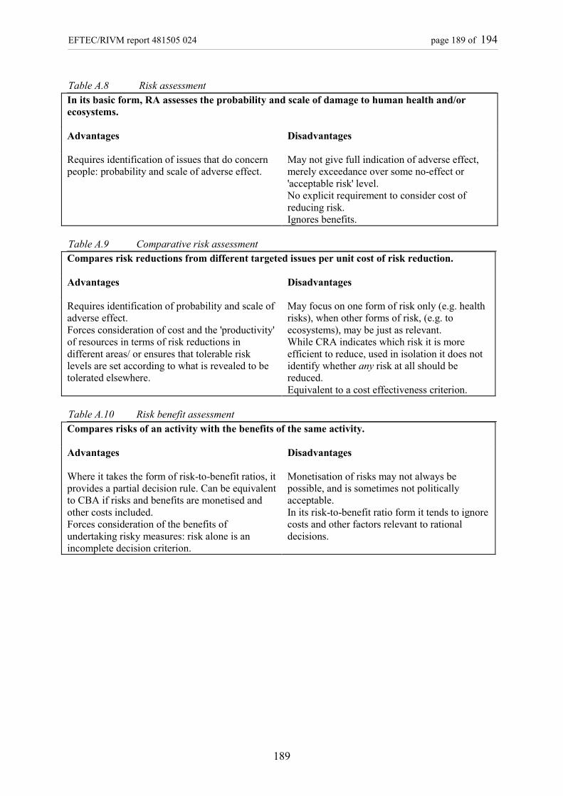
EFTEC/RIVM report 481505 024 page 189 of 194
189
Table A.8 Risk assessmentIn its basic form, RA assesses the probability and scale of damage to human health and/orecosystems.
Advantages Disadvantages
Requires identification of issues that do concernpeople: probability and scale of adverse effect.
May not give full indication of adverse effect,merely exceedance over some no-effect or'acceptable risk' level.No explicit requirement to consider cost ofreducing risk.Ignores benefits.
Table A.9 Comparative risk assessmentCompares risk reductions from different targeted issues per unit cost of risk reduction.
Advantages Disadvantages
Requires identification of probability and scale ofadverse effect.Forces consideration of cost and the 'productivity'of resources in terms of risk reductions indifferent areas/ or ensures that tolerable risklevels are set according to what is revealed to betolerated elsewhere.
May focus on one form of risk only (e.g. healthrisks), when other forms of risk, (e.g. toecosystems), may be just as relevant.While CRA indicates which risk it is moreefficient to reduce, used in isolation it does notidentify whether any risk at all should bereduced.Equivalent to a cost effectiveness criterion.
Table A.10 Risk benefit assessmentCompares risks of an activity with the benefits of the same activity.
Advantages Disadvantages
Where it takes the form of risk-to-benefit ratios, itprovides a partial decision rule. Can be equivalentto CBA if risks and benefits are monetised andother costs included.Forces consideration of the benefits ofundertaking risky measures: risk alone is anincomplete decision criterion.
Monetisation of risks may not always bepossible, and is sometimes not politicallyacceptable.In its risk-to-benefit ratio form it tends to ignorecosts and other factors relevant to rationaldecisions.

page 190 of 194 EFTEC/RIVM report 481505 024
Table A.11 Risk- risk analysisRequires that a risk reduction measure accounts for the risks that may be imposed byresponses to the measure itself, e.g. banning saccharin may increase sugar consumption.
Advantages Disadvantages
Forces consideration of the behavioural responseto policy measures. These may offset riskreductions from the policy in question.
It is an incomplete decision rule since it ignorescost.It may also focus exclusively on health risks,but need not do so. A regulation might pass anRRA test but not a CBA test.Once additional risks are introduced, e.g.ecosystem risks, some procedure foraggregation is required.
Table A.12 Health-health analysisCompares risks reduced by a policy with the risks associated with the costs of the policy. Costsreduce incomes and lower income associated with higher risks.
Advantages Disadvantages
Forces consideration of the true meaning of costas foregone benefits.
A regulation might pass (fail) an health-healthanalysis test but fail (pass) a CBA test, e.g. livessaved may be > lives lost, but value of net livessaved < cost of policy.The focus is on health alone, but the proceduretends to focus on mortality alone, ignoringmorbidity.Also health benefits arising from employmentdue to the policy are ignored.Slight real income changes are unlikely to resultin significant reductions in risk aversionexpenditures.
Table A.13 Multi-criteria analysisCompares costs of policy to sets of ‘outputs’ that are not necessarily measured in money terms.
Advantages Disadvantages
Enables quantitative and qualitative data to becombined. Permits explicit trade-off situations tobe identified.Range of impacts wider (multiple goals).Probably cheaper than CBA and morecomprehensive than RA.
No clear criteria for selecting impacts.Risk of double counting impact categories.Potential for arbitrariness in ordinal scoring ofqualitative impacts.Potential for arbitrariness in weighting overallimpacts for relative importance.

EFTEC/RIVM report 481505 024 page 191 of 194
191
Table A.14 Cost effectiveness analysisCompares to costs of measure to some indicator of effectiveness but not in monetary terms.
Advantages Disadvantages
Secures 'value for money' from a given budget.Essential requirement for any rational policy.
Does not say whether a given option isintrinsically worthwhile, merely whether theoption is better than some other option.Becomes MCA if there is more than oneindicator of effectiveness.
Table A.15 Cost Benefit AnalysisAdvantages Disadvantages
Permits determination of 'absolute' desirability ofa policy in economic efficiency terms.Consistent underlying theoretical foundations.Forces consideration of cost as an indicator offoregone benefits (opportunity cost).Consistent with individuals' preferences(democratic base).Explicit treatment of risk and uncertainty viasensitivity analysis, risk-equivalence models,decision - theory etc.
Deals with economic efficiency only, or possiblywith efficiency and distribution only.Tends not to accommodate other policy goals.Potential for discrimination againstsustainability concerns.Data may not permit all benefits and costs to bemonetised.Some public acceptability issues: some pressuregroups continue to see it as 'unethical'.

page 192 of 194 EFTEC/RIVM report 481505 024

EFTEC/RIVM report 481505 024 page 193 of 194
193
Mailing list1-20 Ministry of Economic Affairs, I. Demandt21. Ministry of Economic Affairs, J. Brinkhoff22. Ministry of Economic Affairs, B. Witmond23. Ministry of Economic Affairs, M. Witvliet24. Ministry of Finance, G. Huiskamp25. Ministry of Transport, Public Works and Watermanagement, C. Hiddink,26-35 Ministry of Housing, Spatial Planning and the Environment, K. Vijverberg
36. VROM, DGM, directeur SB, J.H. Enter37. VROM, DGM, SB, C.M. Moons38. EU, DG Environment, M. Vankeukelen39. EU, DG Environment, M. Vainio40. CPB, Den Haag, C. Koopmans41. TK PvdA fractie, R. Pol
42. Depot Nederlandse Publikaties en Nederlandse Bibliografie43. Directeur milieu, N.D. van Egmond44. Directeur sector 5, F. Langeweg45. MNV, R.J.M. Maas46. MNV, O.J. van Gerwen47. MNV, S. Kruitwagen48. MNV, B. Strengers49. MNV, B. de Haan50. MNV, A. de Moor51. LAE, J.A. Hoekstra52. LAE, J.A. Annema53. LAE, R.F.J.M. Engelen54. LAE, A.M. Idenburg55. LAE, A.H. Hanemaaijer56. LAE, H. Nijland57. LAE, L. Brandes58. LLO, J. van Dam59. LLO, J. Jabben60. LLO, J. Beck61. LEO, L. van Bree62. LBM, E. Franssen63. LBM, E. van Kempen64. LBM, A. Dusseldorp65. LBM, M. Marra66. LWD, L. van Liere
67. EFTEC, A. Howarth68. EFTEC, D.W. Pearce

page 194 of 194 EFTEC/RIVM report 481505 024
69. EFTEC, E. Ozdemiroglu70. EFTEC, T. Seccombe-Hett71. MNV, K. Wieringa72. MNV, A.E.M. de Hollander73. MNV, C.M. Streefkerk74-84 EFTEC85. SBD/Voorlichting & Public Relations86. Bureau Rapportenregistratie87. Bibliotheek RIVM88-104 Reserve copies105-123 Bureau Rapportbeheer


