Research Computing with Python, Lecture 7, Numerical Integration … · Research Computing with...

Research Computing with Python, Lecture 7, NumericalIntegration and Solving Ordinary Differential Equations

Ramses van Zon

SciNet HPC Consortium

November 26, 2013

Ramses van Zon (SciNet HPC Consortium) Research Computing with Python, Lecture 7, Numerical Integration and Solving Ordinary Differential EquationsNovember 26, 2013 1 / 31

Today’s Lecture

Numerical Integration

Ordinary Differential Equations

Little bit of theory

How to do this in Python(spoiler: use scipy.integrate)



I =∫D f(x) ddx


Numerical Integration Methods

If our integral cannot be computed exactly, what options do we have?

.Method depends on dimension d,function f(x), and x-domain..

d=1: Regular gridGaussianQuadrature

d small: Regular gridRecursiveQuadrature

d� 1: Monte Carlo

.


Regularly spaced grid methods

Problem:

A curve is given by anfunction y=f(x).The area under the curve isrequired, between a and b.

Numerical approach:

Compute the value of y atequally space points xUsing an interpolationfunction between thosepoints, compute area

In the figure:

Linear interpolation:trapezoidal ruleThe shaded area is returnedby this approachThis is an approximation tothe actual area.


Equally spaced grid approach

Compute the value of y atequally space points x

Trapezoidal rule:

I =1

2y1 +

n−1∑i=2

yi +1

2yn

def f(x):

return cos(x/9)*sin(x)**2

a=0

b=10

x=linspace(a,b,40)

dx=x[1]-x[0]

y=f(x)*dx

I1=(y[0]+y[-1])/2+sum(y[1:-1])

print I1

3.93845493792


Different evenly spaced grid approaches

Trapezoidal ∫ a+h

a

f(x) dx ≈h

2[f(a) + f(a + h)]

Simpson

∫ a+2h

a

f(x) dx ≈ h

[1

3f(a) +

4

3f(a +

h

2) +

1

3f(a + h)

]Bode, Backward differentiation, . . .

Different prefactors, different orders, different points

What you use is the extension of these rules to

multiple intervals.


Unevenly spaced gridsGaussian quadrature

Based on orthogonal polynomials on the interval.E.g. Legendre, Chebyshev, Hermite, Jacobi polynomialsCompute and yi = f(xi) then∫ b

a

f(x) dx ≈n∑

i=1

vifi

xi and vi from polynomial propertiesTend to be more accurate than equally spaced approaches

# nth order Gauss-Legendre quadrature:

from scipy.integrate import fixed_quad

I2=fixed_quad(f,a,b,n=20)[0]

print I2

3.9363858769075524


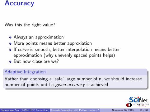
Accuracy

Was this the right value?

Always an approximationMore points means better approxiationIf curve is smooth, better interpolation means betterapproximation (why unevenly spaced points helps)But how close are we?

Adaptive Integration

Rather than choosing a ‘safe’ large number of n, we should increasenumber of points until a given accuracy is achieved


Adaptive Integration

#Adaptive Gauss-Legendre integration

from scipy.integrate import quad

I3=quad(f,a,b,epsrel=0.001)

print I3

(3.936385876907544, 0.0009622632189420763)

Arguments of interest for quad

f: The function

a,b: The x limits

epsabs: Absolute error tolerance.

epsrel: Relative error tolerance.

limit : An upper bound on the number of subintervals used inthe adaptive algorithm.


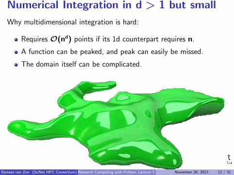
Numerical Integration in d > 1 but small

Why multidimensional integration is hard:

Requires O(nd) points if its 1d counterpart requires n.

A function can be peaked, and peak can easily be missed.

The domain itself can be complicated.


Numerical Integration in d > 1 but small

So what should you do?

If you can reduce the d byexploiting symmetry or doingpart of the integralanalytically, do it!

If you know the function tointegrate is smooth and itsdomain is fairly simple, youcould do repeated 1dintegrals (fixed-grid orGaussian quadrature)

Otherwise, you’ll have toconsider Monte Carlo.

from scipy.integrate import dblquad

def f(x,y):

return x*y

def y1(x):

return 0

def y2(x):

return 3.14

a=0; b=3.14

I4=dblquad(f,a,b,y1,y2)

print I4[0]

24.30292804


Monte Carlo Integration

Use random numbers to pick points at which to evaluate integrand.

Convergence always as 1/√

n, regardless of d.Simple and flexible.


Monte Carlo Integration

You can find python packages for MC (not in scipy, though)

But the essence is the same:

1 Use random numbers to generate points in your domain2 Evaluate the function on those points3 Average them and compute standard deviation for error.

One variation is to use a bias in step 1 to focus on regions ofinterest. Bias can be undone in averaging step

Another variation is to have each point generated from theprevious one plus a random component: MC chain.


Ordinary Differential Equations


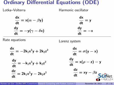
Ordinary Differential Equations (ODE)

Lotka–Volterra

dx

dt= x(α− βy)

dy

dt= −y(γ − δx)

Harmonic oscillator

dx

dt= y

dy

dt= −x

Rate equations

dx

dt= −2k1x2y + 2k2z2

dy

dt= −k1x2y + k2z2

dz

dt= 2k1x2y − 2k2z2

Lorenz system

dx

dt= σ(y − x)

dy

dt= x(ρ− z)− y

dz

dt= xy − βz


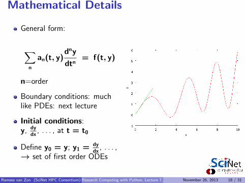
Mathematical Details

General form:

∑n

an(t, y)dny

dtn= f(t, y)

n=order

Boundary conditions: muchlike PDEs: next lecture

Initial conditions:y, dy

dx, . . . , at t = t0

Define y0 = y; y1 = dydx

, . . . ,→ set of first order ODEs


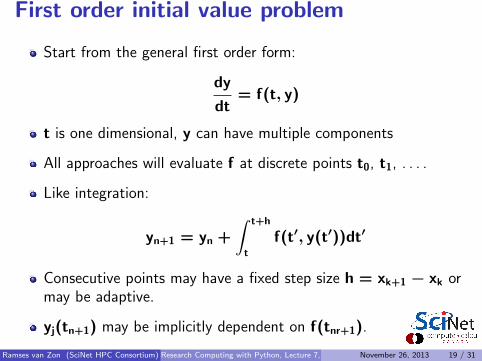
First order initial value problem

Start from the general first order form:

dy

dt= f(t, y)

t is one dimensional, y can have multiple components

All approaches will evaluate f at discrete points t0, t1, . . . .

Like integration:

yn+1 = yn +

∫ t+h

t

f(t′, y(t′))dt′

Consecutive points may have a fixed step size h = xk+1 − xk ormay be adaptive.

yj(tn+1) may be implicitly dependent on f(tnr+1).


Stiff ODEs

A stiff ODE is one that is hard to solve, i.e. requiring a very smallstepsize h or leading to instabilities in some algoritms.

Usually due to wide variation of time scales in the ODEs.

Not all methods equally suited for stiff ODEs. Implicit ones tendto be better for stiff problems.


ODE solver algorithms: Euler

To solve:dy

dt= f(t, y)

Simple approximation:

yn+1 ≈ yn + hf(tn, yn) “forward Euler′′

Rationale:

y(tn + h) = y(tn) + hdy

dt(tn) +O(h2)

So:y(tn + h) = y(tn) + hf(tn, yn) +O(h2)

O(h2) is the local error.For given interval [t1, t2], there are n = (t2 − t1)/h stepsGlobal error: n×O(h2) = O(h)Not very accurate, nor very stable (next): don’t use.


Stability

Example: solve harmonic oscillator numerically:

dx

dt= y

dy

dt= −x

Using Euler gives(xn+1

yn+1

)=

(1 h−h 1

)(xn

yn

)

Stability: eigenvalues λ± = 1± ih of that matrix.

|λ±| =√

1 + h2 > 1 ⇒ Unstable for any h!


ODE algorithms: implicit mid-point Euler

To solve:dy

dt= f(t, y)

Symmetric simple approximation:

yn+1 ≈ yn + hf(xn, (yn + yn+1)/2) “mid-point Euler′′

This is an implicit formula, i.e., has to be solved for yn+1.

Example: Harmonic oscillator

(1 −h

2h2

1

)(y

[1]n+1

y[2]n+1

)=

(1 h

2

−h2

1

)(y[1]

n

y[2]n

)

Eigenvalues M are λ± = (1±ih/2)2

1+h2/4so |λ±| = 1⇒ Stable


ODE solver algorithms: Predictor-Corrector

Computation of new point

Correction using that new point

Gear P.C.: keep previous values of y to do higher order Taylorseries (predictor), then use f in last point to correct. Can sufferfrom catestrophic cancellation at very low h.

Adams: Similarly uses past points to compute.

Runge-Kutta: Refines by using mid-points.

Some schemes require correction until convergence.

Some schemes can use the jacobian, e.g. the derivatives of theright hand side.


Further ODE solver techniques

Adaptive methods:

As with the integration, rather than taking a fixed h, vary h such thatthe solution has a certain accuracy.

Don’t code this yourself!

Good schemes are implemented in packages such asscipy.integrate.odeint, scipy.integrate.ode

odeint uses an Adams integrator for non-stiff problems, and abackwards differentiation method for stiff problem.

ode is a bit more flexible.


Lotka–Volterra using scipy.integrate.odeint

dx

dt= x(α− βy)

dy

dt= −y(γ − δx)

from scipy.integrate\import odeint

alpha=0.1

beta=0.015

gamma=0.0225

delta=0.02

def system(z,t):

x,y=z[0],z[1]

dxdt= x*(alpha-beta*y)

dydt=-y*(gamma-delta*x)

return [dxdt,dydt]

t=linspace(0,300.,1000)

x0,y0=1.0,1.0

sol=odeint(system,[x0,y0],t)

X,Y=sol[:,0],sol[:,1]

plot(X,Y)


Conclusions


Conclusions

Many different methods for numerical integration and solvingODEs

Python package scipy.integrate helps you out.

It has procedures to readily get good results:scipy.integrate.quad and scipy.integrate.odeint

Unfortunately, hard to get what they really do:

I For scipy.integrate.quad, had to look into the scipy python sourceto know that it uses Legendre polynomials.

I For scipy.integrate.odeint, had to look into the fortrandocumentation

If you’re using sciPy for anything but exploration: do youresearch and learn what they really do!


Next Time


Next and Final Lecture

Thursday November 28, 2013, 11:00 amTopic: Partial differential equations


Research Computing with Python, Lecture 7, Numerical Integration … · Research Computing with...

Documents

Transcript of Research Computing with Python, Lecture 7, Numerical Integration … · Research Computing with...