Research Article Supply Chain Network Design under Demand...
16
Research Article Supply Chain Network Design under Demand Uncertainty and Supply Disruptions: A Distributionally Robust Optimization Approach Ruozhen Qiu and Yizhi Wang School of Business Administration, Northeastern University, No. 195, Chuangxin Road, Hunan New District, Shenyang, Liaoning 110169, China Correspondence should be addressed to Ruozhen Qiu; [email protected] Received 24 May 2016; Revised 6 August 2016; Accepted 22 September 2016 Academic Editor: Xiaofeng Xu Copyright © 2016 R. Qiu and Y. Wang. is is an open access article distributed under the Creative Commons Attribution License, which permits unrestricted use, distribution, and reproduction in any medium, provided the original work is properly cited. We develop a robust optimization model for designing a three-echelon supply chain network that consists of manufacturers, distribution centers, and retailers under both demand uncertainty and supply disruptions. e market demands are assumed to be random variables with known distribution and the supply disruptions caused by some of the facilities faults or connection links interruptions are formulated by several scenarios with unknown occurrence probabilities. In particular, we assume the probabilities that the disruption scenarios happen belong to the two predefined uncertainty sets, named box and ellipsoid uncertainty sets, respectively. rough mathematical deductions, the proposed robust SCN design models can be transformed into the tractable linear program for box uncertainty and into second-order cone program for ellipsoid uncertainty. We further offer propositions with proof to show the equivalence of the transformed problems with the original ones. e applications of the proposed models together with solution approaches are investigated in a real case to design a tea supply chain network and validate their effectiveness. Numerical results obtained from model implementation and sensitivity analysis arrive at important practical insights. 1. Introduction Designing and managing a supply chain network have become crucial due to the increasing market competition, variable customer demands, and the fast development of the economic and technological globalization. An efficient supply chain network will contribute to quickly responding to the customers’ demands and achieving the success of the supply chain which depends on the cooperation and coordination among all members. Supply chain network (SCN) design incorporates both strategic and tactical deci- sions on the number, location, capacity, and mission of the supply, production, and distribution facilities required to provide goods to a customer base [1]. In recent years, lots of mathematical models have been developed to solve various supply chain network design problems. A. Nagurney and L. S. Nagurney [2] consider a firm that is engaged in determining the capacities of its various supply chain activities and develop a rigorous modelling and analytical framework for the design of sustainable supply chain networks. Bashiri et al. [3] present a mathematical model for strategic and tactical planning in a multiple-echelon, multiple-commodity production-distribution network. Mahdi et al. [4] indicate the SCN design can significantly affect the economic viability of a biofuel technology and develop a mixed-integer linear programming to determine the optimal supply chain design and operation under uncertain environment. Jeihoonian et al. [5] adopt a mixed-integer programming model to design a closed-loop supply chain network for durable goods and coordinate forward flow and reverse flow to determine the position of each type of facilities in the entire network. For comprehensive reviews of SCN design models, see Klibi et al. [6], Tokman and Beitelspacher [7], and Farahani et al. [8]. By investigating the supply chain models, Melo et al. [9] find that both strategic and tactical decisions can be highly affected by various sources of uncertainty such as demand and supply interruptions, lead time variability, exchange rate volatility, and capacity variations [10]. From the perspective Hindawi Publishing Corporation Scientific Programming Volume 2016, Article ID 3848520, 15 pages http://dx.doi.org/10.1155/2016/3848520
-
Upload
hoangduong -
Category
Documents
-
view
215 -
download
0
Transcript of Research Article Supply Chain Network Design under Demand...
Research ArticleSupply Chain Network Design under DemandUncertainty and Supply Disruptions A DistributionallyRobust Optimization Approach
Ruozhen Qiu and Yizhi Wang
School of Business Administration Northeastern University No 195 Chuangxin Road Hunan New DistrictShenyang Liaoning 110169 China
Correspondence should be addressed to Ruozhen Qiu rzqiumailneueducn
Received 24 May 2016 Revised 6 August 2016 Accepted 22 September 2016
Academic Editor Xiaofeng Xu
Copyright copy 2016 R Qiu and Y WangThis is an open access article distributed under the Creative Commons Attribution Licensewhich permits unrestricted use distribution and reproduction in any medium provided the original work is properly cited
We develop a robust optimization model for designing a three-echelon supply chain network that consists of manufacturersdistribution centers and retailers under both demand uncertainty and supply disruptions The market demands are assumed tobe random variables with known distribution and the supply disruptions caused by some of the facilities faults or connection linksinterruptions are formulated by several scenarios with unknown occurrence probabilities In particular we assume the probabilitiesthat the disruption scenarios happen belong to the two predefined uncertainty sets named box and ellipsoid uncertainty setsrespectively Through mathematical deductions the proposed robust SCN design models can be transformed into the tractablelinear program for box uncertainty and into second-order cone program for ellipsoid uncertainty We further offer propositionswith proof to show the equivalence of the transformed problems with the original ones The applications of the proposed modelstogether with solution approaches are investigated in a real case to design a tea supply chain network and validate their effectivenessNumerical results obtained from model implementation and sensitivity analysis arrive at important practical insights
1 Introduction
Designing and managing a supply chain network havebecome crucial due to the increasing market competitionvariable customer demands and the fast development ofthe economic and technological globalization An efficientsupply chain network will contribute to quickly respondingto the customersrsquo demands and achieving the success ofthe supply chain which depends on the cooperation andcoordination among all members Supply chain network(SCN) design incorporates both strategic and tactical deci-sions on the number location capacity and mission of thesupply production and distribution facilities required toprovide goods to a customer base [1] In recent years lots ofmathematical models have been developed to solve varioussupply chain network design problems A Nagurney and L SNagurney [2] consider a firm that is engaged in determiningthe capacities of its various supply chain activities anddevelop a rigorous modelling and analytical framework for
the design of sustainable supply chain networks Bashiriet al [3] present a mathematical model for strategic andtactical planning in a multiple-echelon multiple-commodityproduction-distribution network Mahdi et al [4] indicatethe SCN design can significantly affect the economic viabilityof a biofuel technology and develop a mixed-integer linearprogramming to determine the optimal supply chain designand operation under uncertain environment Jeihoonian etal [5] adopt a mixed-integer programming model to designa closed-loop supply chain network for durable goods andcoordinate forward flow and reverse flow to determine theposition of each type of facilities in the entire network Forcomprehensive reviews of SCN design models see Klibi et al[6] Tokman and Beitelspacher [7] and Farahani et al [8]
By investigating the supply chain models Melo et al [9]find that both strategic and tactical decisions can be highlyaffected by various sources of uncertainty such as demandand supply interruptions lead time variability exchange ratevolatility and capacity variations [10] From the perspective
Hindawi Publishing CorporationScientific ProgrammingVolume 2016 Article ID 3848520 15 pageshttpdxdoiorg10115520163848520
2 Scientific Programming
of risk management Tang [11] defines two categories ofrisks in supply chains One is operational risks arising frombusiness-as-usual incidents such as machine breakdownsand power outages which lead to uncertainties in matchingsupply and demand The second category is disruptionrisks which arise from natural and man-made disasterssuch as earthquakes floods hurricanes and terrorist attacksOperational risks are usually captured through incorporat-ing such inherent uncertainties in the input data such asuncertain customer demand uncertain supply capacity anduncertain costs due to dynamic and fluctuating nature ofthese parameters Disruption risks are usually captured byincorporating disruption scenarios in the model formulationof underlying decision problem since they are unlikely tooccur but have a high impact when they do occur [12] Tocope with the disadvantage effect of the uncertainties onsupply chain operations Klibi et al [6] suggest that stochas-tic programming can be used as a powerful technique totackle uncertainties Furthermore a so-called scenario-basedstochastic programminghas beenpaidmore attention in SCNdesign problems Scenario-based stochastic programmingoptimizes the expected value of the objective functions byconsidering a set of discrete scenarios and their occurrenceprobabilities for random variables Following such logicMulvey et al [13] initially propose a scenario-based robuststochastic optimization for large-scale systems and definetwo measures of robustness namely model robustness andsolution robustness respectively A solution to an optimiza-tion model is defined as robust solution if it remains closeto optimal for all scenarios of the input data and robustmodel if it remains almost feasible for all data scenarios Byusing a parameter reflecting the decision-makerrsquos preferencebetween the solution and model robustness it incorporatesthe conflicting objectives of the two The scenario-basedrobust optimization can be regarded as a two-stage stochasticprogramming in essence and has been adopted as an effectivetool for designing and managing the supply chain operatingin uncertain environments
Using the robust optimization approach proposed byMulvey et al [13] Babazadeh and Razmi [14] develop anefficient mixed-integer linear programming to handle bothoperational and disruption risks of the agile supply chainnetwork Baghalian et al [15] consider both demand-side andsupply-side uncertainties and develop a stochastic mathe-matical formulation for designing a network of multiproductsupply chains Jabbarzadeh et al [16] present a dynamicsupply chain network design model for the supply of bloodduring and after disasters which can assist in blood facilitylocation and allocation decisions for multiple postdisasterperiods Jeong et al [17] provide an integrated framework todesign emergency logistics networks comprising distributionwarehouses disaster recovery centers and neighbourhoodlocations based on efficiency risk and robustness met-rics where the efficiency and risk are determined usingtransportation cost and relief item loss cost while therobustness is analyzed in terms of perturbed transportationcost through diverse damage scenarios to major facilitiesFattahi and Govindan [18] apply a two-stage stochastic pro-gram to address a multistage and multiperiod supply chain
network design problem under stochastic and highly variabledemands
Applications of robust stochastic programming tech-niques for SCN design models are limited because of theshortage of historical data for fitting probability distributionsfor uncertain parameters [19] According to Klibi et al[6] stochastic programming techniques usually require theperfect information of probability distributions of randomvariables such as the likelihood of an interruption occurrenceand its magnitude of impact Such historical data especiallyfor those rare events is limited or nonexistent making itdifficult or impossible to estimate the actual distribution ofuncertain parameters [20] A robust optimization approachwhich depends on the complete distributions of the ran-dom variables on no condition could be adopted to handleuncertain parameters Soyster [21] was the first to intro-duce a robust optimization formulation with interval datauncertainty which will lead to the overconservative solutionsbecause the probability at which uncertain parameters reachtheir worst values is as low as that at which they reach theirnormal values Subsequently Ben-Tal and Nemirovski [22]Bertsimas and Sim [23] and Ben-Tal et al [24 25] reducethe conservation of Soysterrsquos approach by well defining theuncertainty sets to which the uncertain parameters belongand can thus be applied to design the robust supply chainnetwork Pishvaee et al [26] assume the demand and thereturns of used products vary in a specified closed boundedbox and propose a robust optimization model for handlingthe inherent uncertainty of input data in a closed-loop supplychain network design problem Hasani et al [19] proposea general comprehensive model for strategic closed-loopsupply chain network design in which the uncertainties ofparameters such as demand and purchasing cost in the pro-posed model are handled via an interval robust optimizationtechnique Hatefi and Jolai [27] propose a robust and reliablemodel for an integrated forward-reverse logistics networkdesign which simultaneously takes uncertain parameters andfacility disruptions into account More recently Hasani etal [28] propose a robust optimization model based on theuncertainty budget concept to consider uncertain parametersin global supply chain network design Akbari and Karimi[29] use the similar robust optimization approach to designa multiechelon multiproduct multiperiod supply chain net-work under process uncertainty Hasani andKhosrojerdi [30]develop a mixed-integer nonlinear model and consider sixflexible and resilience strategies simultaneously in designingrobust global supply chain networks under disruptions anduncertainties In addition they present an efficient parallelTaguchi-based memetic algorithm to solve the proposedmodel
From the literatures mentioned above it can be seenthat the disruption issues have drawn attention in SCNdesign problems However both demand uncertainty andsupply disruption are rarely considered simultaneously [1531] especially for the unknown disruption occurrence prob-ability In this paper we develop a path-based three-echelonrobust SCN design model under both demand and supplyuncertainties For the uncertain market demand we assumewithout the loss of generality it is a random variable with
Scientific Programming 3
a known distribution such as normal distribution whichmaylead to a nonlinear model To improve the solving efficiencya piecewise linearization method is applied to transformthe nonlinear terms into the linear ones For the supplyuncertainty we consider some supply disruption scenarioscaused by the manufacturersrsquo facilities faults or the pathinterruption between the supply chain nodes In particularwe use two predefined uncertainty sets named box andellipsoid respectively to describe the unknown probabilitiesthat the disruption scenarios happen which motivates usto adopt the robust optimization to build the SCN designmodels Furthermore through mathematical operations allformulated robust optimization models are transformed intotractable convex programs and can thus be solved efficiently
The remainder of this paper is organized as follows Webriefly introduce the SCN design problem under demanduncertainty and supply disruption in Section 2 and thenpropose a SCN design model in Section 3 In Section 4 weproposed two robust SCNdesignmodelswhen the disruptionscenarios probabilities are bounded in the box uncertaintyset and ellipsoid uncertainty set respectively We furthertransform them into the tractable linear and second-ordercone programs to solve A case study is given in Section 5 toillustrate the proposed models and solutions and to confirmtheir effectiveness In the last section we summarize thepaper and discuss future research directions
2 Problem Description
In this paper we focus on the SCN design of a three-echelon supply chain under both the demand uncertaintyand supply disruptions The supply chain involves somepotential manufactures distribution centers and retailerslocated in some candidate locations of the markets As themarket terminals the retailers are in charge of the sellingand face uncertain market demands that are considered asrandom variables with known distribution Before observingthe market demands retailers need to place orders from theupstream The distribution centers integrate the orders fromthe retailers and pass them to the manufacturers To achieveeconomies of scale themanufactures are inclined to integratethe orders and then organize production or purchase fromthe outer suppliers Once the goods are produced and readyfor shipment they will be transported to distribution centersby consolidation and then arranged for delivery to multipledestinations To meet the requirement of each market across-dock operation can be adopted in the distributioncenters to replenish fast-moving store inventories
Figure 1 depicts the basic network structure We alsouse the concept of a path or route instead of defining flowvariables among the nodes of the supply chain [15] Thuseach link starting from a manufacturer passing through adistribution center and ending at a retailer can be regardedas a potential transportation route We further considerdisruption risks in supply chain which impose great impactson the companiesrsquo performance According to Azad et al[32] sources of disruption risks can be segmented into twocategories random disruption risks which may occur at any
I1
I2
IN119868
J1
J2
JN119869
M1
M2
Mm
MN119872
Manufacturers Distribution centers Retailersmarkets
Figure 1 The three-echelon supply chain network
physical point of supply chain network for example naturalhazards and earthquakes and premeditated disruption riskswhich are deliberately planned to inflict the supply chain withmaximum damages
In this paper we mainly aim to explore the SCN designunder premeditated disruption risks In particular we con-sider the supply disruptions due to the manufacturersrsquo facil-ities impairments or connection links interruptions whichresult in some of the potential routes being unusable Thedisruption set caused by a specific event is called a scenarioand is assigned with a finite but unknown probability ofoccurrence which is remarkably different from the literatureswith the assumption of knowing the scenarios occurrenceprobability
We propose a robust SCN design model incorporatingboth the demand uncertainty and supply disruptions todetermine supply chain networks and operation strategiesthat can perform well under all scenarios Two types ofdecision variables are considered in the proposedmodel Oneinvolves numbers and locations of the distribution centersor retailers and is named the first-stage decision variablesThe other concerns the product flow along the differentroutes and is named the second-stage decision variables Theformer are used to determine the network structure while thelatter match with the operation strategiesThus the proposedrobust SCN design models can be considered as two-stagerobust optimization problems
3 Mathematical Formulations
The sets parameters and variables used in the formulation ofthe robust SCN design model are defined in the Notations
The expected profit of eachmarket119898 in scenario 119904 is givenby
119864 [120587119904119898] = 119864[[sum119901isin119875119875119898119901 sdotmin sum119903isin119877119898
119876119901119904119903 119863119898119901
+ sum119901isin119875
119881119898119901 sdot ( sum119903isin119877119898
119876119901119904119903 minus 119863119898119901)+ minus sum119901isin119875
119862119898119901
4 Scientific Programming
sdot (119863119898119901 minus sum119903isin119877119898
119876119901119904119903)+ minus sum119901isin119875
sum119903isin119877119898
119867119901119903 sdot 119876119901119904119903]]= sum119901isin119875
(119875119898119901 + 119862119898119901) sum119903isin119877119898
119876119901119904119903minus sum119901isin119875
(119875119898119901 + 119862119898119901 minus 119881119898119901)intsum119903isin119877119898 1198761199011199041199030
119865 (119863119898119901) 119889119863119898119901minus sum119901isin119875
119862119898119901 sdot 119864 [119863119898119901] sdot 120577119898 minus sum119901isin119875
sum119903isin119877119898
119867119901119903 sdot 119876119901119904119903(1)
where 119909+ = max119909 0 and 119864[sdot] represents the expectationoperator Note that the supply disruptions caused by theimpairments of the manufacturerrsquos facilities or the inter-ruptions of the connection links are taken into account bydefining several scenarios In each scenario some of thepotential routes are unavailable Therefore the SCN designmodel incorporating the demand uncertainty and supplydisruptions can be described as
max Π= sum119904isin119878
119901119904( sum119898isin119872
sum119901isin119875
(119875119898119901 + 119862119898119901) sum119903isin119877119898
119876119901119904119903 minus sum119898isin119872
sum119901isin119875
(119875119898119901 + 119862119898119901 minus 119881119898119901) intsum119903isin119877119898 1198761199011199041199030
119865 (119863119898119901) 119889119863119898119901 minus sum119898isin119872
sum119901isin119875
119862119898119901sdot 119864 [119863119898119901] sdot 120577119898 minussum
119901isin119875
sum119903isin119877119898
119867119901119903 sdot 119876119901119904119903) minussum119895isin119869
119866119895 sdot 120581119895 minus sum119898isin119872
119871119898 sdot 120577119898(2)
st sum119901isin119875
119876119901119904119903 le 119882 sdot 119861119904119903 forall119904 isin 119878 119903 isin 119877 (3)
sum119901isin119875
sum119903isin119877
119876119901119904119903 le 119882 sdot 120581119895 forall119904 isin 119878 119895 isin 119869 (4)
sum119901isin119875
sum119903isin119877
119876119901119904119903 le 119882 sdot 120577119898 forall119904 isin 119878 119898 isin 119872 (5)
sum119895isin119869
119866119895 sdot 120581119895 + sum119898isin119872
119871119898 sdot 120577119898 le 119910 (6)
sum119903isin119877119894
119876119901119904119903 le 119876max119894119901 forall119894 isin 119868 119901 isin 119875 119904 isin 119878 (7)
119876119901119904119903 ge 0 forall119901 isin 119875 119904 isin 119878 119903 isin 119877 (8)
120581119895 120577119898 isin 0 1 forall119895 isin 119869 119898 isin 119872 (9)
Objective function (2) aims to maximize the whole supplychain networkrsquos expected profit under all the scenarios Con-straint (3) represents that the products can only be distributedalong the feasible routes in the network in each scenario119904 where 119882 is a given big positive Constraints (4) and (5)impose the capacity restrictions on the located facilitiesConstraint (6) implies that the cost expense of locating thefacilities in the network cannot exceed the budget Constraint(7) imposes the amount of product 119901 shipped along route119903 isin 119877119894 that should be less than the maximum capacityof manufacturer 119894 Constraint (8) means the product flowin the network is positive Constraint (9) includes twobinary variables used to decide whether a facility should beestablished
Problems (2)ndash(9) cannot be solved efficiently due to thenonlinear term intsum119903isin119877119898 119883119901119904119903
0119865(119863119898119901)119889119863119898119901 in (2) For example
if the demand follows a normal distribution calculating thisterm is not straightforward since the integral of cumulativedistribution function cannot be a closed form We use apiecewise linear transformation to convert the nonlinearfunction into a linear one in each interval divided by goldensection method The linearized function is not exactly thesame as the original nonlinear one which will result in anerror between the two However the error can be decreasedby increasing the number of intervals Figure 2 shows thelinearization approximation process of continuous nonlinearfunction 119891(119909) (119909 isin [119909119897 119909119906] 119871 = 119909119906 minus 119909119897) Let 1199091 = 119909119897
Scientific Programming 5
0 xl xu x
L
xl + 0618L
f(x)
xl + 0618iL
Figure 2 Piecewise linearization of a nonlinear function
and 1199101 = 119891(1199091) we then obtain the first golden section ratio1199092 = 1199091 +0618 sdot119871 corresponding to a function value 1199102 and alinear equation119910 = 119896(119909minus1199091)+1199101with slope 119896 = (1199102minus1199101)(1199092minus1199091) = (1199102 minus 1199101)(0618 sdot 119871) on the interval [1199091 1199092] Similarlywe have the 119894th golden section ratio 1199092 = 1199091 + 0618119894 sdot 119871 whenstarting from the initial point1199091 and the corresponding linearequation119910 = 119896119894(119909minus1199091)+1199101 with the slope 119896119894 = (1199102minus1199101)(1199092minus
1199091) = (1199102minus1199101)(0618119894 sdot119871) Consider the fitting error denotedby 120576 = 119910minus119891(119909) = 119896119894(119909minus1199091) +1199101 minus119891(119909) Themaximum error120576max is achieved at 119889120576119889119909 = 119896119894minus1198911015840(119909) = 0The linear equation119910 = 119896119894(119909minus1199091)+1199101 can be used to approximately substitute thenonlinear term on the interval [1199091 1199092] if the maximum erroris allowable Otherwise we can continue to consider (119894 + 1)thgolden section ratio Let 1199092 be an initial point and followthe process above to perform the next linearization untilwe get the piecewise linear functions on the whole interval[119909119897 119909119906]
Let 119899119898 isin 119873119898 = 1 2 signify the set of approximationintervals for each market 119898 and define 119886119899119898 and 119887119899119898 asthe slope coefficient and intercept of the linear functionfor interval 119899119898 of market 119898 respectively Besides 119906119899119898and 119889119899119898 are specified to represent the lower and upperbounds for interval 119899119898 of market 119898 The decision variable119876119901119904119903 can thus be replaced with 119876119899119898119901119904119903 which expressesthe amount of product 119901 shipped along route 119903 in sce-nario 119904 for the interval 119899119898 Therefore the SCD designmodel (2)ndash(9) can be reformulated as the following linearprogram
max sum119904isin119878
119901119904 sdot 120587119904 minussum119895isin119869
119866119895 sdot 120581119895 minus sum119898isin119872
119871119898 sdot 120577119898 (10)
st 120587119904= sum119898isin119872
sum119901isin119875
(119875119898119901 + 119862119898119901) sdot sum119903isin119877119898
sum119899119898isin119873119898
119876119899119898119901119904119903 minus sum119898isin119872
sum119901isin119875
(119875119898119901 + 119862119898119901 minus 119881119898119901) sum119899119898isin119873119898
(119886119899119898 sum119903isin119877119898
119876119899119898119901119904119903 + 119887119899119898120579119899119898119901119904)minus sum119898isin119872
sum119901isin119875
119862119898119901 sdot 119864 [119863119898119901] sdot 120577119898 minus sum119901isin119875
sum119903isin119877119898
119867119901119903 sdot sum119899119898isin119873119898
119876119899119898119901119904119903 forall119904 isin 119878(11)
sum119898isin119872
sum119899119898isin119873119898
sum119901isin119875
sum119903isin119877119895
119876119899119898119901119904119903 le 119882 sdot 120581119895 forall119895 isin 119869 forall119904 isin 119878 (12)
sum119898isin119872
sum119899119898isin119873119898
sum119901isin119875
sum119903isin119877119898
119876119899119898119901119904119903 le 119882 sdot 120577119898 forall119898 isin 119872 forall119904 isin 119878 (13)
sum119898isin119872
sum119899119898isin119873119898
sum119903isin119877119894
119876119899119898119901119904119903 le 119880119894119901 forall119894 isin 119868 forall119901 isin 119875 forall119904 isin 119878 (14)
sum119895isin119869
119866119895 sdot 120581119895 + sum119898isin119872
119871119898 sdot 120577119898 le 119910 (15)
sum119899119898isin119873119898
120579119899119898119901119904 = 1 forall119901 isin 119875 forall119904 isin 119878 (16)
sum119903isin119877119898
119876119899119898119901119904119903 le 119906119899119898 sdot 120579119899119898119901119904 forall119899119898 isin 119873119898 forall119904 isin 119878 forall119901 isin 119875 (17)
sum119903isin119877119898
119876119899119898119901119904119903 ge 119889119899119898 sdot 120579119899119898119901119904 forall119899119898 isin 119873119898 forall119904 isin 119878 forall119901 isin 119875 (18)
119876119899119898119901119904119903 ge 0 forall119899119898 isin 119873119898 forall119901 isin 119875 forall119904 isin 119878 forall119903 isin 119877 (19)
120579119899119898119901119904 isin 0 1 forall119899119898 isin 119873119898 forall119901 isin 119875 forall119904 isin 119878 (20)
120581119895 120577119898 isin 0 1 forall119895 isin 119869 forall119898 isin 119872 (21)
6 Scientific Programming
where 120587119904 is an auxiliary variable introduced to simplify themodel descriptionNote that the binary variable 120579119899119898119901119904 is equalto 1 if interval 119899119898 is selected for product 119901 in market119898 underscenario 119904 and 0 otherwise Constraint (16) ensures that onlyone interval can be selected for eachmarket Constraints (17)-(18) indicate the amount of product 119901 of each interval isrestricted by its boundary Other constraints are explicatedas shown above
The optimal profit of the whole supply chain in thereal scenario may differ from the objective function valuederived from the proposed mathematical model we intro-duce the solution robustness defined in Mulvey et al [13] toreduce the deviation and make the SCN design model morerobust
max sum119904isin119878
119901119904 sdot 120587119904 minus 120582sum119904isin119878
119901119904 sdot (120587119904 minus sum1199041015840isin119878
1199011199041015840 sdot 1205871199041015840)2
minussum119895isin119869
119866119895 sdot 120581119895 minus sum119898isin119872
119871119898 sdot 120577119898st constraints (11) ndash (21)
(22a)
where 120582 denotes the weight used to measure the solutionvarianceThe objective value of problem (22a) is less sensitiveto change in the input data under all scenarios as thevariable weight 120582 increases However the quadratic termsum119904isin119878 119901119904(120587119904 minus sum1199041015840isin119878 11990111990410158401205871199041015840)2 which evaluates the closeness ofa solution to optimality for 119904 isin 119878 usually requires a largecomputation time Yu and Li [33] suggest that the quadraticterm can be replaced with sum119904isin119878 119901119904|120587119904 minus sum1199041015840isin119878 11990111990410158401205871199041015840 | By theapproach proposed in Yu and Li [33] problem (22a) can beconverted into the following equivalent linear formulation
max sum119904isin119878
119901119904 sdot 120587119904 minus 120582sum119904isin119878
119901119904sdot [(sum1199041015840isin119878
1199011199041015840 sdot 1205871199041015840 minus 120587119904) + 2120596119904] minussum119895isin119869
119866119895 sdot 120581119895minus sum119898isin119872
119871119898 sdot 120577119898st sum
119904isin119878
119901119904 sdot 120587119904 minus 120587119904 + 120596119904 ge 0 forall119904 isin 119878120596119904 ge 0 forall119904 isin 119878constraints (11) ndash (21)
(22b)
Note that if sum1199041015840isin119878 1199011199041015840 sdot 1205871199041015840 minus 120587119904 ge 0 forall119904 isin 119878 the maximizationobjective requires 120596119904 = 0 otherwise 120596119904 = 120587119904 minus sum119904isin119878 119901119904 sdot 120587119904due to the first constraint of problem (22b) Therefore thesolution of problem (22b) is similar to that of problem (22a)when the quadratic termsum119904isin119878 119901119904(120587119904minussum1199041015840isin119878 11990111990410158401205871199041015840)2 is replacedby sum119904isin119878 119901119904|120587119904 minus sum1199041015840isin119878 11990111990410158401205871199041015840 | Obviously problem (22b) is alinear program and can thus be solved efficiently when theprobability of the disruption occurrence of scenario 119904 isin 119878 isknown However it is difficult or impossible to estimate theactual distribution of uncertain parameters due to the lack
of the historical data especially for those rare events [20] Inthe next section we will further discuss the situation that theaccurate probability of supply disruption is unavailable
4 Robust SCN Design Model under UncertainSupply Disruption Probability
Assume the probability distribution of the supply disruptionis not complete and only known to belong to an uncertain setP with pr isin P pr = (1199011 1199012 119901119873119878)119879 The robust counter-part of problem (22b) can be formulated as
maxΘ120596
minprisinP
sum119904isin119878
119901119904 sdot 120587119904 minus 120582sum119904isin119878
119901119904sdot [(sum1199041015840isin119878
1199011199041015840 sdot 1205871199041015840 minus 120587119904) + 2120596119904] minussum119895isin119869
119866119895sdot 120581119895 minus sum
119898isin119872
119871119898 sdot 120577119898st min
prisinPsum119904isin119878
119901119904 sdot 120587119904 ge 120587119904 minus 120596119904 forall119904 isin 119878120596119904 ge 0 forall119904 isin 119878constraints (11) ndash (21)
(23)
where Θ isin 119877119873119889 denotes the set of the decision variablesand 120596 = (1205961 1205962 120596119873119878)119879 is the auxiliary vector [33] Notethat problem (23) cannot be solved directly due to the minoperators in both objective function and the first constraintIn the following we introduce two uncertainty sets namelybox and ellipsoid Problem (23) can thus be transformedinto a linear program and a second-order cone programrespectively
41 Robust SCN Design Model under Box Uncertainty Thebox uncertainty set to which the probability of the supplydisruption scenario belongs is defined as follows
pr isin P119868 ≜ pr | pr = p + 120585 e119879120585 = 0 120585 le 120585 le 120585 (24)
where p = (1199011 1199012 119901119873119878)119879 is a nominal distribution thatrepresents the most likely distribution of the disruptionprobability 120585 isin [120585 120585] denotes the uncertain parameter vectorand e signifies the vector of one The constraint e119879120585 =0 ensures pr will meet the requirement of the probabilitydistribution
Let us first consider the following max-min optimizationproblem in (24)
maxΘ120596
minprisinP119868
(120587 minus 2120582120596)119879 pr minus 119891 (25)
where120587 = (1205871 1205872 120587119873119878)119879 and119891 = sum119895isin119869 119866119895 sdot120581119895+sum119898isin119872 119871119898 sdot120577119898 The inner minimization problem is
minprisinP119868
(120587 minus 2120582120596)119879 pr minus 119891= (120587 minus 2120582120596)119879 p +G
lowast (120585) minus 119891 (26)
Scientific Programming 7
whereGlowast(120585) is the optimal value of the following problem
min120585
(120587 minus 2120582120596)119879 120585 | e119879120585 = 0 120585 le 120585 le 120585 (27)
The dual program of (27) can be described as follows
max120575120591^
120585119879120591 + 120585119879^ | e120575 + 120591 + ^ = 120587 minus 2120582120596 120591 le 0 ^ ge 0 (28)
According to the linear programming duality theory itcan be seen that the optimal value of the objective functionin problem (27) is equal to that in (28) Following the similarmathematic process the left-hand side of the first constraintin (23) is given by
minprisinP119868120587119879pr
= min120585
120587119879p + 120587119879120585 | e119879120585 = 0 120585 le 120585 le 120585= 120587119879p +R
lowast (120585) (29)
whereRlowast(120585) is the optimal value of min120585120587120585 | e119879120585 = 0 120585 le120585 le 120585 which has the following dual problem
max120574120572120573
120585119879120572 + 120585119879120573 | e120574 + 120572 + 120573 = 120587 120572 le 0 120573 le 0 (30)
Now consider the following optimization problem
maxΘ120596120575120591^120574120572120573
(120587 minus 2120582120596)119879 p + 120585119879120591 + 120585119879^ minus 119891st e120575 + 120591 + ^ = 120587 minus 2120582120596
e120574 + 120572 + 120573 = 120587120587119879p + 120585119879120572 + 120585119879120573 ge 120587119904 minus 120596119904 forall119904 isin 119878120591 le 0 ^ ge 0 120572 le 0 120573 ge 0120596119904 ge 0 forall119904 isin 119878constraints (11) ndash (21)
(31)
Proposition 1 shows that solving (23) under boxuncertainty is equivalent to solving (31) with variables(Θ120596 120575 120591 ^ 120574120572120573) isin 119877119873119889 times 119877 times 119877119873119878 times 119877119873119878 times 119877 times 119877119873119878 times 119877119873119878 Proposition 1 If the solution (Θlowast120596lowast 120575lowast 120591lowast ^lowast 120574lowast120572lowast120573lowast)solves (31) then the solution (Θlowast120596lowast) solves (23) with P =P119868 and conversely if the solution (Θlowast120596lowast) solves (23) withP = P119868 then (Θlowast120596lowast 120575lowast 120591lowast ^lowast 120574lowast120572lowast120573lowast) solves (31)where (120575lowast 120591lowast ^lowast) and (120574lowast120572lowast120573lowast) are the optimal solutionsof (28) and (30) respectively
Proof Let (Θlowast120596lowast 120575lowast 120591lowast ^lowast 120574lowast120572lowast120573lowast) be a solution to (31)then (120575lowast 120591lowast ^lowast) and (120574lowast120572lowast120573lowast) would be feasible to (28)and (30) respectively Assuming there exists another solution(Θlowast lowast) to problem (23) such that Υ(Θlowast120596lowast) lt Υ(Θlowast lowast)
where Υ(Θ120596) = minprisinP119868(120587 minus 2120582120596)119879pr minus 119891 we can obtain(lowast lowast lowast) and (lowast lowast lowast) by solving (28) and (30) respec-tively It can be seen that (Θlowast lowast lowast lowast lowast lowast lowast lowast) isalso feasible to (30) Since the objective functions of (23)and (31) have the same form it contradicts the assumptionthat (Θlowast120596lowast 120575lowast 120591lowast ^lowast 120574lowast120572lowast120573lowast) is a solution to (31) due toΥ(Θlowast120596lowast) lt Υ(Θlowast lowast) Therefore (Θlowast120596lowast) is a solution to(23)
Conversely if (Θlowast120596lowast) is optimal to (23) then (120575lowast 120591lowast ^lowast)and (120574lowast120572lowast120573lowast) would be solutions to (28) and (30) respec-tively Obviously (Θlowast120596lowast 120575lowast 120591lowast ^lowast 120574lowast120572lowast120573lowast) is also a fea-sible solution to problem (31) If there exists a differentsolution (Θlowast lowast lowast lowast lowast lowast lowast lowast) to (31) then from thediscussion of the first part of the proof (Θlowast lowast) is an optimalsolution to (23) which contradicts the assumption that(Θlowast120596lowast) solves (23) Hence (Θlowast120596lowast 120575lowast 120591lowast ^lowast 120574lowast120572lowast120573lowast)solves (31)
Clearly problem (31) is a linear program and can thusbe solved efficiently In particular problem (31) is reducedto a stochastic optimization problem with known disruptionoccurrence probability when 120585 = 120585 = 0 Note that if 120585 ge 0we can increase the value of p to attain 120585 lt 0 Hence we canalways make sure that 120585 lt 0 and 120585 gt 0 hold The constraints
120591 le 0 and ^ ge 0 in (31) imply that the term 120585119879120591 + 120585119879^
is a negative reflecting the performance loss caused by theuncertainty
42 Robust SCN Design Model under Ellipsoid UncertaintyThe ellipsoid uncertainty set to which the probability of thesupply disruption scenario belongs is defined as follows
pr isin P119864 ≜ pr | pr = p + A120585 p + A120585 ge 0 e119879A120585= 0 120585 le 1 (32)
where p is the most likely distribution which is the center ofthe ellipsoid sdot is the Euclidean norm and sdot lowast is its dualrepresentation Due to the self-duality of Euclidean norm wehave sdot lowast = sdot A isin 119877119899times119899 is a known scaling matrixto measure the degree of the uncertainty The constraintse119879A120585 = 0 and p + A120585 ge 0 ensure that the vector pr is aprobability distribution Hence the objective of problem (23)can be formulated as follows
maxΘ120596
minprisinP119864
(120587 minus 2120582120596)119879 pr minus 119891 (33)
Consider the following inner optimization problem ofproblem (33)
minprisinP119864
(120587 minus 2120582120596)119879 pr minus 119891= (120587 minus 2120582120596)119879 p + Q
lowast (120585) minus 119891 (34)
8 Scientific Programming
where Qlowast(120585) is the optimal value of the following problem
min120585
(120587 minus 2120582120596)119879A120585 | p + A120585 ge 0 e119879A120585 = 0 120585 le 1 (35)
It can be seen that problem (35) is a second-order coneprogramwith the variable vector 120585 and its Lagrange is definedas
L (120578 120588 120583 120585) = (120587 minus 2120582120596)119879A120585 + 120578119879 (minusp minus A120585)+ 120588 (120585 minus 1) + 120583e119879A120585 (36)
The Lagrange dual function with (120578 120588 120583) isin 119877119873119878 times 119877 times 119877 isgiven by
119892 (120578 120588 120583) = min120585
L (120578 120588 120583 120585) = (minusp119879120578 minus 120588)minusmax120585
(minusA119879 (120587 minus 2120582120596) + A119879120578 minus A119879e120583)119879 120585minus 120588 120585 = (minusp119879120578 minus 120588) minus Λlowast (minusA119879 (120587 minus 2120582120596)+ A119879120578 minus A119879e120583)
(37)
where Λlowast(y) = 0 ylowast le 120588 infin ylowast gt 120588 is the conjugatefunction of Λ(120585) = 120588120585 Then the Lagrange dual problemassociated with problem (35) is given by
max120578120588120583
119892 (120578 120588 120583) = max120578120588120583
minusp119879120578 minus 120588 | 10038171003817100381710038171003817minusA119879 (120587 minus 2120582120596) + A119879120578 minus A119879e12058310038171003817100381710038171003817 le 120588 120578 ge 0 120588 ge 0 (38)
Obviously problem (38) is a concave program According tothe characteristic of a probability distribution there existsa disturbance vector 120585 such that p + A120585 gt 0 whichmeans Slaterrsquos condition holds Therefore in light of thestrong duality theorem of Lagrange problem (34) is equiv-alent to the following maximization problem with variables(Θ120596 120578 120588 120583) isin 119877119873119889 times 119877119873119878 times 119877119873119878 times 119877 times 119877maxΘ120578120588120583
(120587 minus 2120582120596)119879 p minus p119879120578 minus 120588 minus 119891st 10038171003817100381710038171003817minusA119879 (120587 minus 2120582120596) + A119879120578 minus A119879e12058310038171003817100381710038171003817 le 120588
120578 ge 0 120588 ge 0(39)
Following the logic above we have the equivalent formulationof the left-hand side of the first constraint in (23) as follows
minprisinP119864120587119879pr = min
120585120587119879p + 120587119879A120585 | p + A120585
ge 0 e119879A120585 = 0 120585 le 1 = 120587119879p +Hlowast (120585)
(40)
where Hlowast(120585) is the optimal value of min120585120587119879A120585 | p + A120585 ge0 e119879A120585 = 0 120585 le 1 which is equivalent to the followingdual program
max120572120574120573
minusp119879120572 minus 120573 | 10038171003817100381710038171003817minusA119879120587 + A119879120572 minus A119879e12057410038171003817100381710038171003817 le 120573 120572 ge 0 120573 ge 0 (41)
Consider the following optimal problem with variables(Θ120596 120578 120588 120583120572 120573 120574) isin 119877119873119889 times119877119873119878 times119877119873119878 times119877times119877times119877119873119878 times119877times119877maxΘ120596120578120588120583120572120573120574
(120587 minus 2120582120596)119879 p minus p119879120578 minus 120588 minus 119891st 10038171003817100381710038171003817minusA119879 (120587 minus 2120582120596) + A119879120578 minus A119879e12058310038171003817100381710038171003817 le 120588
10038171003817100381710038171003817minusA119879120587 + A119879120572 minus A119879e12057410038171003817100381710038171003817 le 120573120587119879p minus p119879120572 minus 120573 ge 120587119904 minus 120596119904 forall119904 isin 119878120578 ge 0 120572 ge 0 120588 ge 0 120573 ge 0120596119904 ge 0 forall119904 isin 119878Constraints (11) minus (21)
(42)
Proposition 2 shows that solving (23) under ellipsoid uncer-tainty is equivalent to solving (42)
Proposition 2 If the solution (Θlowast120596lowast 120578lowast 120588lowast 120583lowast120572lowast 120573lowast 120574lowast)solves (42) then (Θlowast120596lowast) solves (23) with P = P119864 andconversely if the solution (Θlowast120596lowast) solves optimization problem(23) withP = P119864 then (Θlowast120596lowast 120578lowast 120588lowast 120583lowast120572lowast 120573lowast 120574lowast) solvesoptimization problem (42) where (120578lowast 120588lowast 120583lowast) and (120572lowast 120573lowast 120574lowast)are the optimal solutions of (39) and (41) respectively
The proof of Proposition 2 is omitted because it is similarto that of Proposition 1 Obviously problem (42) is a second-order cone program and can thus be solved efficiently In par-ticular (42) is reduced to a stochastic optimization problemwith known disruption occurrence probability when 120585 = 120585 =0 Similarly it can be observed that the uncertainty of the
Scientific Programming 9
Huzhou City Jiaxing City
Hangzhou City
Shaoxing City
Quzhou CityJinhua City
Wenzhou City
Lishui City
Ningbo City
Zhoushan City
Taizhou City
ManufacturerDistribution centerRetailer
SSShaoxingSh iii
Figure 3 The potential supply chain network structure of CFCompany
disruption occurrence probability will lead to a performanceloss (positive) that is p119879120578 + 1205885 Case Study and Numerical Results
To verify the effectiveness of the proposed robust SCNdesign models and solution approaches we consider a three-tiered supply chain network design for a real-life companyin Hangzhou City of China named CF Company whichmanufactures and sales superior packed Longjing tea TheLongjing tea produced in the surrounding mountains of theLongjing village has efficacies of refreshing producing salivaand slaking thirst reducing blood lipids lowering cholesteroland so on Longjing tea is usually picked and processed fromMarch to May every year and priced from a few hundred tothousands of yuans due to the different picking time and pro-cessing technology Due to the intense competition in localmarket CF Company has to reduce the price and improvethe service quality to meet the target customer group whichhowever leads to a high operation cost in return To dealwith the dilemma that the company faces it is necessaryto design an efficient and reliable supply chain network InFigure 3 we illustrate the potential supply chain networkstructure of CF Company who has three available plantsin Hangzhou three potential distribution centers locatedat candidate locations of Hangzhou Shaoxing and Jiaxingrespectively and eleven potential retailers located succes-sively in Hangzhou Ningbo Wenzhou Shaoxing HuzhouJiaxing Jinhua Quzhou Taizhou Lishui and Zhoushan
There are twelve feasible routes in the potential supplychain network with handling costs given in Table 1 After
Table 1 The unit handling cost on potential routes
Potential route Unit handlingcost (119867119901119903) Potential
routeUnit handlingcost (119867119901119903)1199031minus1minus1 8151 1199032minus2minus9 81541199031minus1minus5 8153 1199032minus3minus3 81551199031minus2minus2 8152 1199033minus1minus8 81591199031minus3minus7 8153 1199033minus2minus11 81581199032minus1minus6 8153 1199033minus3minus9 81561199032minus2minus4 8152 1199033minus3minus10 8152
119903119894minus119895minus119898 dentoes a route starting from manufacturer 119894 to retailer119898 by passingthrough distribution center 119895
Table 2 The distribution of the demand for each market
Market Distribution(1) Hangzhou 1198631 sim 119873 (119864 (1198631) = 700 120590 (1198631) = 5)(2) Ningbo 1198632 sim 119873 (119864 (1198632) = 700 120590 (1198632) = 5)(3) Wenzhou 1198633 sim 119873 (119864 (1198633) = 600 120590 (1198633) = 5)(4) Shaoxing 1198634 sim 119873 (119864 (1198634) = 500 120590 (1198634) = 5)(5) Huzhou 1198635 sim 119873 (119864 (1198635) = 300 120590 (1198635) = 5)(6) Jiaxing 1198636 sim 119873 (119864 (1198636) = 300 120590 (1198636) = 5)(7) Jinhua 1198637 sim 119873 (119864 (1198637) = 600 120590 (1198637) = 5)(8) Quzhou 1198638 sim 119873 (119864 (1198638) = 200 120590 (1198638) = 4)(9) Taizhou 1198639 sim 119873 (119864 (1198639) = 500 120590 (1198639) = 5)(10) Lishui 11986310 sim 119873 (119864 (11986310) = 200 120590 (11986310) = 4)(11) Zhoushan 11986311 sim 119873 (119864 (11986311) = 220 120590 (11986311) = 5)
a series of processes such as picking spreading fixingshaping and drying the production of Longjing tea iscompleted and then packed into finished products (500 gper box) The unit prices of the product for all markets are965 965 966 965 965 965 965 966 965 966 and 966respectively The unit shortage cost for unmet demand is101 and the unit salvage value for residual product is 386The maximum production capacity of each manufacture isconsidered as 2500 2200 and 1200 respectively The fixedcosts for locating distribution centers at candidate locationsof Hangzhou Shaoxing and Jiaxing are 23120 19884 and18888 respectively The fixed costs of locating retailers forthe abovementioned 11 markets are 5780 5676 5517 49714957 4998 4722 4825 5221 4830 and 4943 The budget forestablishing the facilities is 120000 The random demand ofeach market is assumed to follow Gaussian distribution (seeTable 2) Due to confidentiality all the data used in this paperare processed but resemble the data structure ofCFCompany
We consider four possible disruption scenarios due tothe manufacturersrsquo facilities impairments and connectionlinks interruptions In the first scenario all twelve potentialroutes are available which means there is no disruptionoccurring in the supply chain The second and the thirdscenarios are described as only the second and the thirdfacility break down respectively And in the fourth scenariothe second and the third facility fail simultaneously Theprobability of each scenario to occur is only known to belong
10 Scientific Programming
(3)
12
3
(1)
(2)
702
278
657
664
289
564
45
182
198
191
595
455
1451 1464
1905
2301
1206
1493
Huzhou City Jiaxing City
Hangzhou City
Shaoxing City
Quzhou CityJinhua City
Wenzhou City
Lishui City
Ningbo City
Zhoushan City
Taizhou City
ManufacturerDistribution centerRetailer
Figure 4 Network structure and operation strategies under p in thefirst scenario
to a specific uncertainty set where themost likely distributionis estimated to be p = (06875 00500 02500 00125)119879
Webreak the range of each targetmarket into ten intervalsand assume p is the real disruption occurrence probabilitydistribution for the purpose of comparing the robust solutionwith the optimal one Models (31) and (42) are solved withLINGO 1100 software and the runs are performed on an IntelCore with 2 Duo CPU at 22GHzThe solutions are obtainedwithin two minutes approximately
51 Results under p By solving (22b) with pr = p and 120582 = 2we obtain the optimal objective function value of 3756473and the corresponding optimal network structures underdifferent scenarios are displayed in Figures 4ndash7 where thenumbers in the boxes and lines represent the manufacturersrsquoproduction quantity distribution centersrsquo transfer amountand markets sales volume From Figure 4 we find that theyields of three manufactures in the first scenario are 23011493 and 1206 respectively All the potential markets areselected and the total quantities shipped to these markets are5000 Figure 5 (Figure 6) shows that the total yield that is3404 (4184) does not reach the maximum capacity in thesecond (third) scenario Compared with the first scenario wefind the production quantity in the second or third scenariois less than that in the first one due to the impairments of themanufacturersrsquo facilities which results in the unmet marketssuch as 3 4 and 6 under the second scenario and markets 810 and 11 under the third scenario Considering that only thefirst facility can be usable we find that only a few markets areselected in the fourth scenario with the total sales volume of2292 (see Figure 7)
(3)
12
3
(1)698
298
698
598198
218
198
1194916
1294
2292
1112
498
Huzhou City Jiaxing City
Hangzhou CityShaoxing City
Quzhou CityJinhua City
Wenzhou City
Lishui City
Ningbo City
Zhoushan City
Taizhou City
ManufacturerDistribution centerRetailer
Figure 5 Network structure and operation strategies under p in thesecond scenario
12
3
(1)
(2)
698
298
698
598
298
498
498
598
1294 1694
1196
2292
1892
Huzhou City Jiaxing City
Hangzhou City
Shaoxing City
Quzhou CityJinhua City
Wenzhou City
Lishui City
Ningbo City
Zhoushan City
Taizhou City
ManufacturerDistribution centerRetailer
Figure 6 Network structure and operation strategies under p in thethird scenario
Scientific Programming 11
12
3
(1)698
298
698
598
966698
598
2292
Huzhou City Jiaxing City
Hangzhou City
Shaoxing City
Quzhou CityJinhua City
Wenzhou City
Lishui City
Ningbo City
Zhoushan City
Taizhou City
ManufacturerDistribution centerRetailer
Figure 7 Network structure and operation strategies under p in thefourth scenario
52 Results under Box Uncertainty In order to test theproposed SCN design model and the solution approachunder box uncertainty let 120585 = 119892 sdot K K isin [KK] K =(minus1 minus02 minus06 minus005)119879 K = (1 02 06 005)119879 119892 = 002and 120582 = 2 By solving problem (31) we obtain the objectivefunction value of 3108265 However when the solutionsderived from (31) are applied to the real distribution p thecorresponding performance turns into 3241674 Comparingwith the optimal value of 3756473 it can be found thatthe uncertainty in disruption scenario occurrence probabilitywill inevitably lead to the performance loss ((3756473 minus3241674)3756473 = 137) Furthermore the loss can beregarded as the maximum cost for decision-makers who arewilling to pay to obtain the complete disruption informationInterestingly by observing the network structures under boxuncertainty we find that only the SCN design plan in thefirst scenario is different from that in the real distributionp (see Figure 8) We can thus conclude that the proposedrobust SCN design model and solution approach performwell under uncertainty In particular the network structureand corresponding operation strategies are consistent withthe optimal case when the supply disruption does occur inthe supply chain
To further investigate the effectiveness of the proposedrobust optimization approach some of the probability dis-tributions are generated according to (24) with p =(06875 00500 02500 00125)119879 and all of them are con-sidered as the real distributions The calculation results aredisplayed in Table 3 where the numbers in the third column
(3)
12
3
(1)
(2)
701
377
764
595
302
564
378
198
208
126
595
1578
2437
1914
1439
655
1839
123
Huzhou City Jiaxing City
Hangzhou City
Shaoxing City
Quzhou CityJinhua City
Wenzhou City
Lishui City
Ningbo City
Zhoushan City
Taizhou City
ManufacturerDistribution centerRetailer
Figure 8 Network structure and operation strategies under boxcertainty in the first scenario
are obtained by applying the robust solutions to each of thereal distributions generated From Table 3 we find that theperformance loss ratios change around 1370 with relativelysmall amplitude which indicates the proposed solutionapproach in this paper is robust to deal with uncertainty indisruption scenario probability distribution
Since the variability weight 120582 places an important rolein measuring the deviation between the robust performancefor any scenario realization and the optimal one moreexperiments are executed to observe the changing tendenciesof the objective performances under different 120582 and thedegree of uncertainty expressed with a parameter 119892 as wellWe obtain the results shown in Figure 9 From Figure 9 wefind that for a given 120582 or 119892 the performance is decreasingwith the degree of the uncertainty or the variability weight120582 However the lower the degree of the uncertainty thesmaller the decreasing amplitude which implies the supplychain manager should gather more information to improvethe forecasting precision of disruption scenario probability
53 Results under Ellipsoid Uncertainty When the probabil-ities that supply disruption scenarios occur belong to theellipsoid uncertainty set defined in (32) we do the similarnumerical simulations as in Section 52 Let A = ℎ sdotE where E is an identity matrix ℎ = 002 and 120582 =2 By solving (42) we obtain the objective function valueof 3313529 The solutions derived from (42) produce aperformance of 3418326 when applying them to the realdistribution p which leads to the performance loss ratio as
12 Scientific Programming
Table 3 Comparisons under different probability distributions under box uncertainty
Scenario probability distribution Optimal objectivefunction value
Objective function value when applyingrobust solutions to a real distribution Performance loss ratio
(07295 00500 02100 00105) 3794220 3190960 1590(07085 00500 02300 00115) 3775346 3216317 1481(06875 00500 02500 00125) 3756473 3241674 1370(06665 00500 02700 00135) 3737599 3267030 1259(06455 00500 02900 00145) 3718726 3292387 1146
00
05
10
15
20
25
30
35
40
45
50
55
60
65
70
75
80
85
90
95
100
times10000
120582
minus6000minus5000minus4000minus3000minus2000minus1000
000100020003000400050006000
Obj
ectiv
e per
form
ance
g = 010
g = 008
g = 006
g = 004
g = 002
g = 000
Figure 9 Sensitivity analysis on 120582 and 119892 under box uncertainty
900 ((3756473 minus 3418326)3756473) Similarly we alsofind that only the network structure and the correspondingoperation strategies in the first scenario (see Figure 10) aredifferent from the optimal case
Similarly in order to further examine the effectiveness ofthe proposed robust optimization approach under ellipsoiduncertainty some more probability distributions are gene-rated according to (32) with p = (06875 00500 0250000125)119879 and regarded as the real distributions Following thesame calculation as above we obtain the results displayedin Table 4 From Table 4 we find that the performance lossratios change closely around 900 which validates the effec-tiveness of the proposed solution approach in dealing withthe distributional uncertainty Moreover the performancechanging tendencies under different variability weight 120582 andthe degree of the uncertainty ℎ are investigated and the resultsare shown in Figure 11 which reveals the similar relationshipsas those found in Figure 9
6 Conclusions
In this paper we develop a robust optimization model fordesigning a supply chain network including manufacturesdistribution centers and retailers under both demand uncer-tainty and supply disruption For uncertain market demandit is assumed to be random and follow a known distributionand a piecewise linearization method is used to transformthe nonlinear model caused by stochastic demand into alinear one For supply disruption it is described by a series
12
3
698
286
695
596
380
587
107
189
308
189
598
1553
2275
1697
1765
1068
1672
382
Huzhou City Jiaxing City
Hangzhou City
Shaoxing City
Quzhou CityJinhua City
Wenzhou City
Lishui City
Ningbo City
Zhoushan City
Taizhou City
ManufacturerDistribution centerRetailer
(2)
(1)
(3)
Figure 10 Network structure and operation strategies under ellip-soid uncertainty in the first scenario
00
05
10
15
20
25
30
35
40
45
50
55
60
65
70
75
80
85
90
95
100
times10000
120582minus3000minus2000minus1000
000100020003000400050006000
Obj
ectiv
e per
form
ance
ℎ = 010ℎ = 008ℎ = 006
ℎ = 004ℎ = 002ℎ = 000
Figure 11 Sensitivity analysis on 120582 and ℎ under ellipsoid uncer-tainty
Scientific Programming 13
Table 4 Comparisons under different probability distributions under ellipsoid uncertainty
Scenario probability distribution Optimal objective functionvalue
Objective function value when applyingrobust solutions to a real distribution Performance loss ratio
(07295 00500 02100 00105) 3794220 3378405 1096(07085 00500 02300 00115) 3775346 3398365 999(06875 00500 02500 00125) 3756473 3418327 900(06665 00500 02700 00135) 3737599 3438287 801(06455 00500 02900 00145) 3718726 3458248 700
of scenarios with unknown probabilities and the correspond-ing robust counterparts are presented under both box andellipsoid uncertainty Through mathematical propositionswe transform the robust SCN design models into tractablelinear program under box uncertainty and into second-ordercone program under ellipsoid uncertainty
The proposedmodel and solution approach are evaluatedin a real case to examine their effectiveness The results showthat the SCN designed by our approach perform well underthe uncertainty in supply disruption scenario probability Inparticular the lower the degree of the uncertainty the betterthe operation performance of the supply chain networkOur robust supply chain design model can be extended tomultiperiod case by incorporating an inventory managementpolicy In addition another interesting direction for futureresearch is to consider other risk measurements such asconditional value at risk (CVaR) and mean CVaR to measurethe performance under uncertainty which would enrich ourmodel
Notations
Sets
119868 Set of manufacturers indexed by 119894119894 isin 119868 = 1 2 119873119868119869 Set of potential distribution centersindexed by 119895 119898 isin 119872 = 1 2 119873119872119872 Set of markets or retailers indexed by119898119898 isin 119872 = 1 2 119873119872119875 Set of products indexed by 119901119901 isin 119875 = 1 2 119873119875119878 Set of disruption scenarios indexed by 119904119904 isin 119878 = 1 2 119873119878119877 Set of routes starting from manufacturerspassing through distribution centers andending at retailers indexed by 119903119903 isin 119877 = 1 2 119873119877119877119894 Set of routes starting from manufacturer 119894119877119895 Set of routes passing through distributioncenter 119895119877119898 Set of routes shipped to market119898
Parameters
119866119895 Fixed cost of establishing distributioncenter 119895
119871119898 Fixed cost of developing market119898119863119898119901 Demand of product 119901 in market119898 whichis a random variable with the mean119864[119863119898119901] and the cumulative distributionfunction 119865(119863119898119901)119880119894119901 Capacity of manufacturer 119894 for product 119901119910 Cost budget for establishing facilities insupply chain network119875119898119901 Unit sales price of product 119901 in market119898119881119898119901 Unit salvage value of unsold product 119901 inmarket119898119862119898119901 Unit shortage cost of the unmet demandfor product 119901 in market119898119867119901119903 Unit handling cost for product 119901 alongroute 119903 including unit production costunit shipping cost and unit storage cost119901119904 Probability of disruption occurrence ofscenario 119904
Decision Variables
119876119901119904119903 Amount of product 119901 shipped along theroute 119903 in scenario 119904120581119895 Binary variable equal to 1 if a distributioncenter is established in location 119895 and 0otherwise120577119898 Binary variable equal to 1 if market119898 isopened and 0 otherwise119861119904119903 Binary variable equal to 1 if route isavailable in scenario 119904 and 0 otherwise
Competing Interests
The authors declare that they have no competing interests
Acknowledgments
This research is partly supported by the National Natural Sci-ence Foundation of China (no 71372186) and FundamentalResearch Funds for the Central Universities (N150604005)
References
[1] W Klibi and A Martel ldquoThe design of robust value-creatingsupply chain networksrdquo OR Spectrum vol 35 no 4 pp 867ndash903 2013
14 Scientific Programming
[2] A Nagurney and L S Nagurney ldquoSustainable supply chain net-work design a multicriteria perspectiverdquo International Journalof Sustainable Engineering vol 3 no 3 pp 189ndash197 2010
[3] M Bashiri H Badri and J Talebi ldquoA new approach to tacticaland strategic planning in productionndashdistribution networksrdquoApplied Mathematical Modelling vol 36 no 4 pp 1703ndash17172012
[4] S Mahdi C G Marti and S Nilay ldquoSupply chain networkdesign and operation systematic decision-making for cen-tralized distributed and mobile biofuel production usingmixed integer linear programming (MILP) under uncertaintyrdquoBiomass and Bioenergy vol 81 no 2 pp 401ndash414 2015
[5] M Jeihoonian M K Zanjani and M Gendreau ldquoAcceleratingBenders decomposition for closed-loop supply chain networkdesign case of used durable products with different qualitylevelsrdquo European Journal of Operational Research vol 251 no3 pp 830ndash845 2016
[6] W Klibi A Martel and A Guitouni ldquoThe design of robustvalue-creating supply chain networks a critical reviewrdquo Euro-pean Journal of Operational Research vol 203 no 2 pp 283ndash293 2010
[7] M Tokman and L S Beitelspacher ldquoSupply chain networksand service-dominant logic suggestions for future researchrdquoInternational Journal of Physical Distribution and LogisticsManagement vol 41 no 7 pp 717ndash726 2011
[8] R Z Farahani S Rezapour TDrezner and S Fallah ldquoCompeti-tive supply chain network design an overview of classificationsmodels solution techniques and applicationsrdquo Omega vol 45no 2 pp 92ndash118 2014
[9] M T Melo S Nickel and F Saldanha-da-Gama ldquoFacilitylocation and supply chain managementmdasha reviewrdquo EuropeanJournal of Operational Research vol 196 no 2 pp 401ndash4122009
[10] M Esmaeilikia B Fahimnia J Sarkis K Govindan A Kumarand JMo ldquoTactical supply chain planningmodels with inherentflexibility definition and reviewrdquoAnnals ofOperations Researchvol 23 no 1 pp 1ndash21 2014
[11] C S Tang ldquoPerspectives in supply chain risk managementrdquoSSRN Electronic Journal vol 103 no 2 pp 451ndash488 2006
[12] N S Sadghiani S A Torabi andN Sahebjamnia ldquoRetail supplychain network design under operational and disruption risksrdquoTransportation Research Part E Logistics amp TransportationReview vol 75 no 1 pp 95ndash114 2015
[13] J M Mulvey R J Vanderbei and S A Zenios ldquoRobustoptimization of large-scale systemsrdquo Operations Research vol43 no 2 pp 264ndash281 1995
[14] R Babazadeh and J Razmi ldquoA robust stochastic programmingapproach for agile and responsive logistics under operationaland disruption risksrdquo International Journal of Logistics Systemsand Management vol 13 no 4 pp 458ndash482 2012
[15] A Baghalian S Rezapour and R Farahani ldquoRobust supplychain network design with service level against disruptionsand demand uncertainties a real-life caserdquo European Journal ofOperational Research vol 227 no 1 pp 199ndash215 2013
[16] A Jabbarzadeh B Fahimnia and S Seuring ldquoDynamic supplychain network design for the supply of blood in disastersa robust model with real world applicationrdquo TransportationResearch Part E Logistics amp Transportation Review vol 70 pp225ndash244 2014
[17] K-Y Jeong J-D Hong and Y Xie ldquoDesign of emergencylogistics networks taking efficiency risk and robustness intoconsiderationrdquo International Journal of Logistics Research andApplications vol 17 no 1 pp 1ndash22 2014
[18] M Fattahi and K Govindan ldquoInvestigating risk and robustnessmeasures for supply chain network design under demanduncertainty a case study of glass supply chainrdquo InternationalJournal of Production Economics 2015
[19] A Hasani S H Zegordi and E Nikbakhsh ldquoRobust closed-loop supply chain network design for perishable goods inagilemanufacturing under uncertaintyrdquo International Journal ofProduction Research vol 50 no 16 pp 4649ndash4669 2012
[20] S Zokaee A Jabbarzadeh B Fahimnia et al ldquoRobust supplychain network design an optimization model with real worldapplicationrdquo Annals of Operations Research vol 21 no 2 pp1ndash30 2014
[21] A L Soyster ldquoConvex programming with set-inclusive con-straints and applications to inexact linear programmingrdquoOper-ations Research vol 21 no 5 pp 1154ndash1157 1973
[22] A Ben-Tal and A Nemirovski ldquoRobust solutions of linearprogramming problems contaminated with uncertain datardquoMathematical Programming Series B vol 88 no 3 pp 411ndash4242000
[23] D Bertsimas and M Sim ldquoThe price of robustnessrdquoOperationsResearch vol 52 no 1 pp 35ndash53 2004
[24] A Ben-Tal A Goryashko E Guslitzer and A NemirovskildquoAdjustable robust solutions of uncertain linear programsrdquoMathematical Programming vol 99 no 2 pp 351ndash376 2004
[25] A Ben-Tal B D Chung S R Mandala and T Yao ldquoRobustoptimization for emergency logistics planning risk mitigationin humanitarian relief supply chainsrdquo Transportation ResearchPart B Methodological vol 45 no 8 pp 1177ndash1189 2011
[26] M S Pishvaee M Rabbani and S A Torabi ldquoA robustoptimization approach to closed-loop supply chain networkdesign under uncertaintyrdquoAppliedMathematicalModelling vol35 no 2 pp 637ndash649 2011
[27] S M Hatefi and F Jolai ldquoRobust and reliable forward-reverselogistics network design under demand uncertainty and facilitydisruptionsrdquo Applied Mathematical Modelling vol 38 no 9-10pp 2630ndash2647 2014
[28] A Hasani S H Zegordi and E Nikbakhsh ldquoRobust closed-loop global supply chain network design under uncertainty thecase of the medical device industryrdquo International Journal ofProduction Research vol 53 no 5 pp 1596ndash1624 2015
[29] A A Akbari and B Karimi ldquoA new robust optimizationapproach for integrated multi-echelon multi-product multi-period supply chain network design under process uncertaintyrdquoInternational Journal of Advanced Manufacturing Technologyvol 79 no 1ndash4 pp 229ndash244 2015
[30] A Hasani and A Khosrojerdi ldquoRobust global supply chainnetwork design under disruption and uncertainty consideringresilience strategies a parallel memetic algorithm for a real-life case studyrdquo Transportation Research Part E Logistics andTransportation Review vol 87 no 1 pp 20ndash52 2016
[31] S Rezapour J K Allen T B Trafalis et al ldquoRobust supply chainnetwork design by considering demand-side uncertainty andsupply-side disruptionrdquo in Proceedings of the ASME Interna-tional Design Engineering Technical Conference V03AT03A030Portland Ore USA August 2013
Scientific Programming 15
[32] N Azad G K D Saharidis H Davoudpour H Maleklyand S A Yektamaram ldquoStrategies for protecting supply chainnetworks against facility and transportation disruptions animproved Benders decomposition approachrdquo Annals of Oper-ations Research vol 210 no 1 pp 125ndash163 2013
[33] C S Yu and H L Li ldquoA robust optimization model forstochastic logistic problemsrdquo International Journal of Produc-tion Economics vol 64 no 1ndash3 pp 385ndash397 2000
Submit your manuscripts athttpwwwhindawicom
Computer Games Technology
International Journal of
Hindawi Publishing Corporationhttpwwwhindawicom Volume 2014
Hindawi Publishing Corporationhttpwwwhindawicom Volume 2014
Distributed Sensor Networks
International Journal of
Advances in
FuzzySystems
Hindawi Publishing Corporationhttpwwwhindawicom
Volume 2014
International Journal of
ReconfigurableComputing
Hindawi Publishing Corporation httpwwwhindawicom Volume 2014
Hindawi Publishing Corporationhttpwwwhindawicom Volume 2014
Applied Computational Intelligence and Soft Computing
thinspAdvancesthinspinthinsp
Artificial Intelligence
HindawithinspPublishingthinspCorporationhttpwwwhindawicom Volumethinsp2014
Advances inSoftware EngineeringHindawi Publishing Corporationhttpwwwhindawicom Volume 2014
Hindawi Publishing Corporationhttpwwwhindawicom Volume 2014
Electrical and Computer Engineering
Journal of
Journal of
Computer Networks and Communications
Hindawi Publishing Corporationhttpwwwhindawicom Volume 2014
Hindawi Publishing Corporation
httpwwwhindawicom Volume 2014
Advances in
Multimedia
International Journal of
Biomedical Imaging
Hindawi Publishing Corporationhttpwwwhindawicom Volume 2014
ArtificialNeural Systems
Advances in
Hindawi Publishing Corporationhttpwwwhindawicom Volume 2014
RoboticsJournal of
Hindawi Publishing Corporationhttpwwwhindawicom Volume 2014
Hindawi Publishing Corporationhttpwwwhindawicom Volume 2014
Computational Intelligence and Neuroscience
Industrial EngineeringJournal of
Hindawi Publishing Corporationhttpwwwhindawicom Volume 2014
Modelling amp Simulation in EngineeringHindawi Publishing Corporation httpwwwhindawicom Volume 2014
The Scientific World JournalHindawi Publishing Corporation httpwwwhindawicom Volume 2014
Hindawi Publishing Corporationhttpwwwhindawicom Volume 2014
Human-ComputerInteraction
Advances in
Computer EngineeringAdvances in
Hindawi Publishing Corporationhttpwwwhindawicom Volume 2014
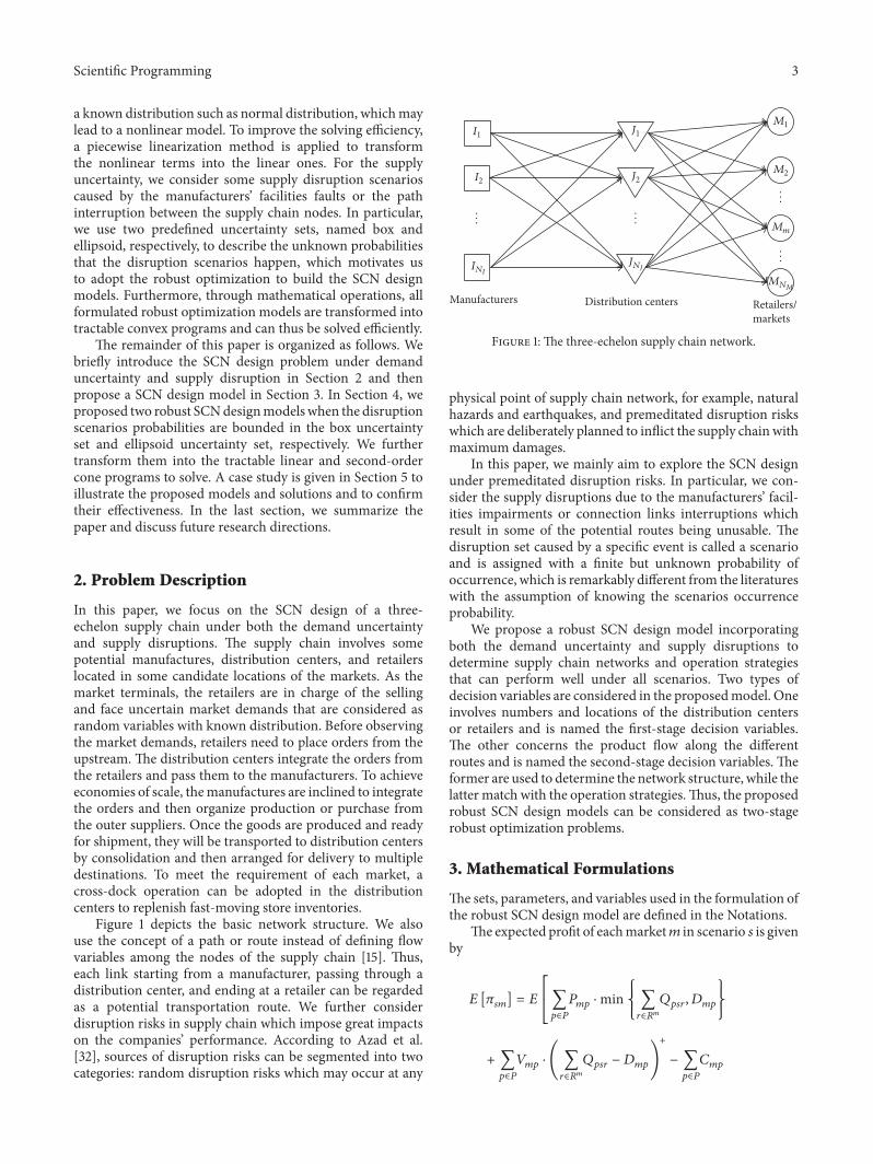
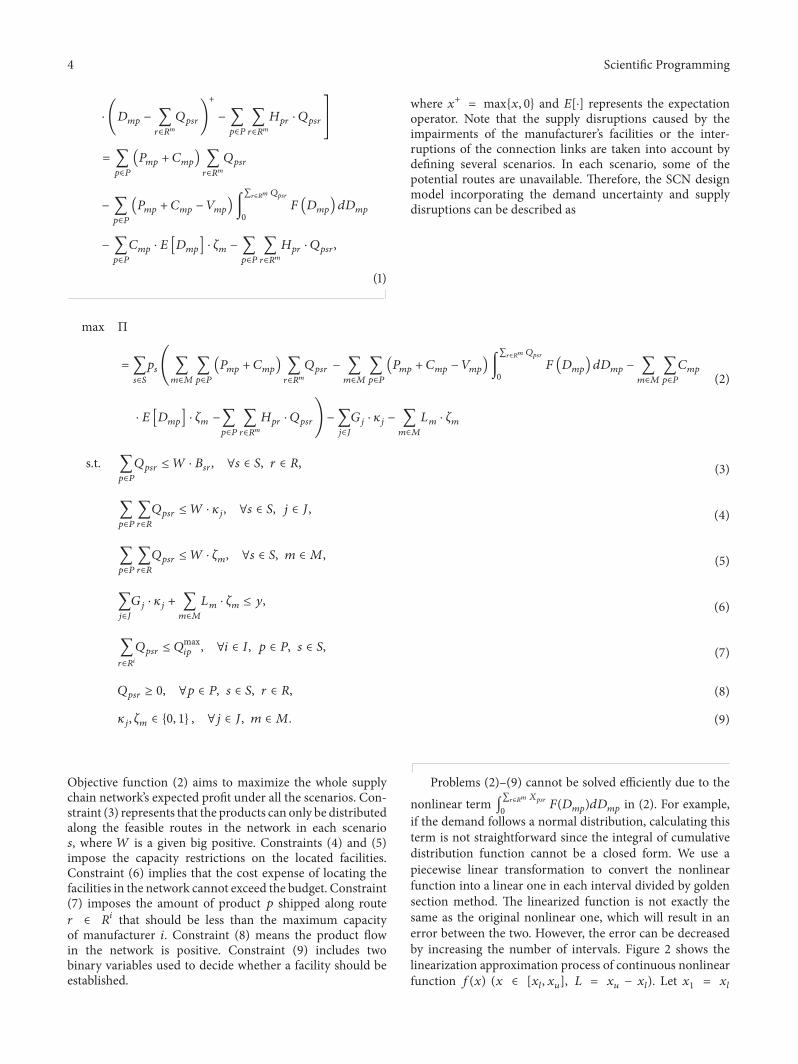
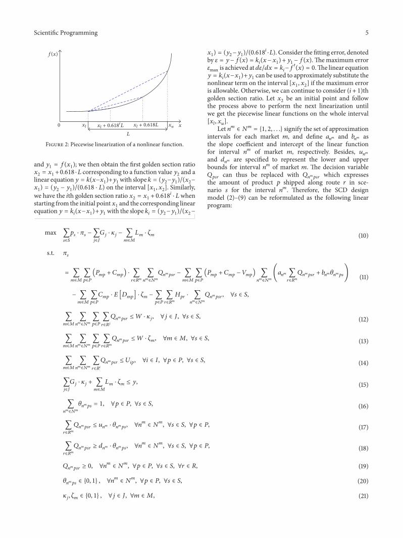
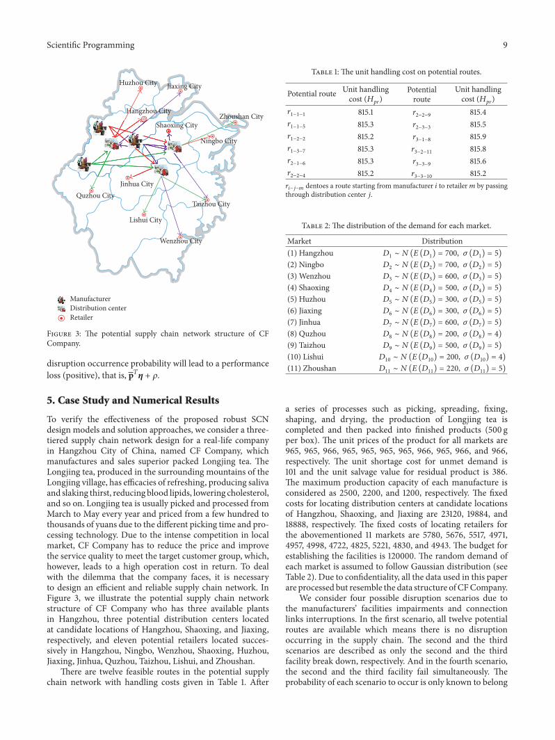
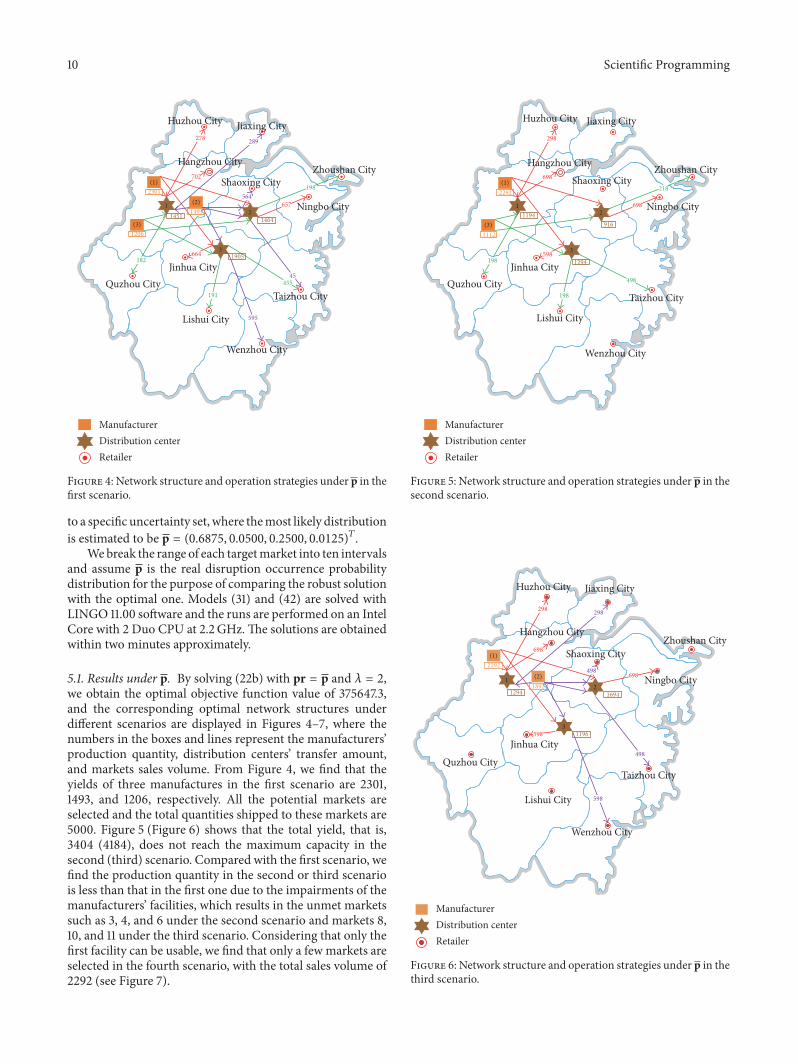
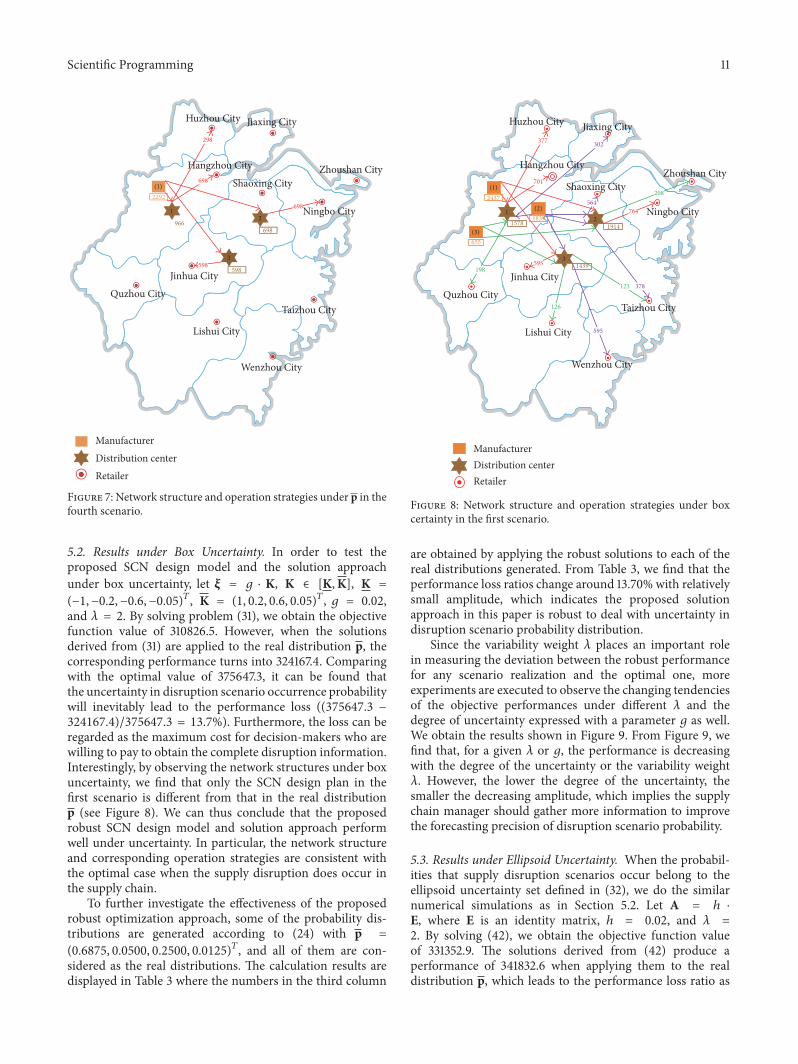
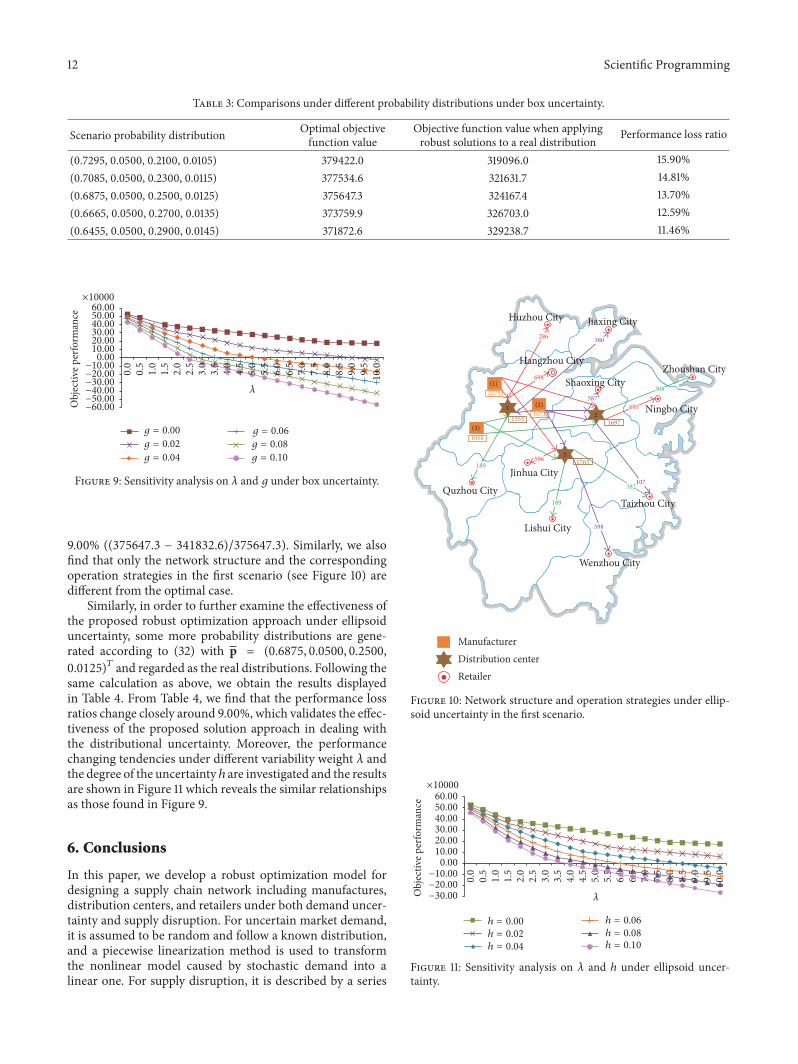
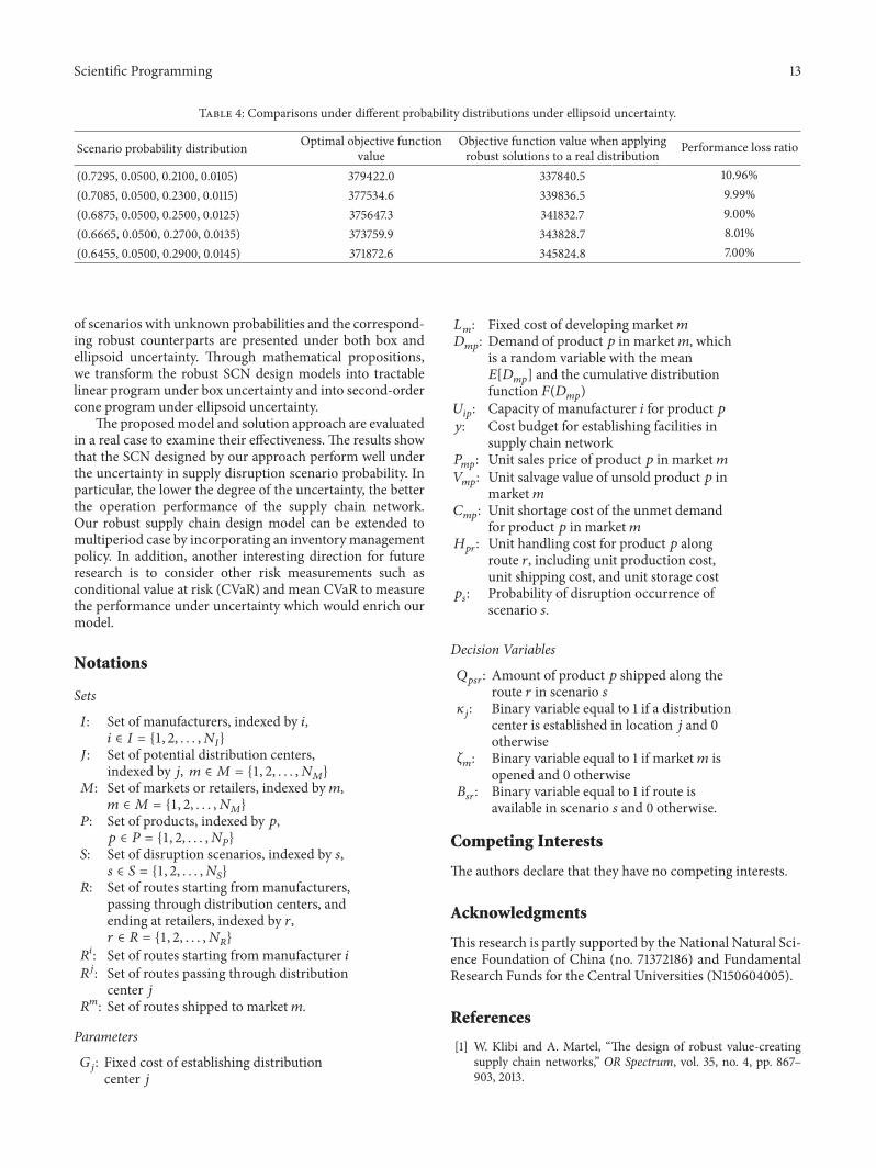
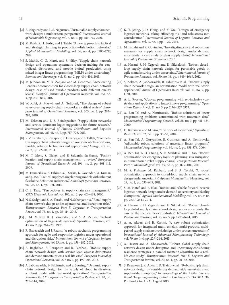