Research Article Direct Torque Control of Sensorless ...
18
Research Article Direct Torque Control of Sensorless Induction Machine Drives: A Two-Stage Kalman Filter Approach Jinliang Zhang, 1 Longyun Kang, 1 Lingyu Chen, 1 Boyu Yi, 1 and Zhihui Xu 2 1 School of Electric Power, South China University of Technology, Guangzhou, Guangdong 510640, China 2 Sunwoda Electronic Corporation Limited, Shenzhen 518108, China Correspondence should be addressed to Jinliang Zhang; [email protected] Received 27 May 2015; Revised 27 August 2015; Accepted 27 August 2015 Academic Editor: Mohamed Djemai Copyright © 2015 Jinliang Zhang et al. is is an open access article distributed under the Creative Commons Attribution License, which permits unrestricted use, distribution, and reproduction in any medium, provided the original work is properly cited. Extended Kalman filter (EKF) has been widely applied for sensorless direct torque control (DTC) in induction machines (IMs). One key problem associated with EKF is that the estimator suffers from computational burden and numerical problems resulting from high order mathematical models. To reduce the computational cost, a two-stage extended Kalman filter (TEKF) based solution is presented for closed-loop stator flux, speed, and torque estimation of IM to achieve sensorless DTC-SVM operations in this paper. e novel observer can be similarly derived as the optimal two-stage Kalman filter (TKF) which has been proposed by several researchers. Compared to a straightforward implementation of a conventional EKF, the TEKF estimator can reduce the number of arithmetic operations. Simulation and experimental results verify the performance of the proposed TEKF estimator for DTC of IMs. 1. Introduction High performance control and estimation techniques for induction machines (IMs) have been finding more and more applications with Blaschke’s well-known field oriented control (FOC) method [1]. To improve the dynamic response of instantaneous electromagnetic torque and simplicity in control structure, one such technique for induction machine control is that the direct torque control (DTC) method can provide accurate fast torque control [2]. is method has become increasingly popular for industrial applications due to the simplified control strategy and lower parameter dependence, in comparison with the FOC methods [3, 4]. For DTC of IMs, the method requires information on the position and amplitude of the controlled stator flux for speed control applications. In the conventional approach, the stator flux is obtained utilizing a search coil or through Hall effect sensors, whilst speed sensors like incremental encoders or resolvers are used to monitor rotor velocity [2]. ese unnecessarily increase hardware costs and the size of the control systems and degrade the reliability of the systems when encountering defective environments. So, sensorless DTC strategy has become the hot issue in research and drawn many researchers and engineers’ attention. Conventional approaches to sensorless DTC of IMs employ the method of stator flux and rotor velocity estima- tion by using a stator voltage model [5, 6]. is method has a large error in rotor velocity estimation, particularly in the low-speed operation range. Some recent studies conducting simultaneous stator flux and rotor velocity estimation for sensorless DTC technology include model reference adap- tive system (MRAS) [7], artificial neural networks (ANN) [8], sliding mode control (SMC) [9], extended Luenberger observer [10], and extended Kalman filter (EKF) [2, 11]. e model uncertainties and nonlinearities inherent to induction motors are well suited to the EKF’s stochastic nature [2]. Using this method, it is possible to make estimation of states whilst simultaneously performing identification of parameters in a short time [12–14], even taking measurement and system noises directly into system model. is explains why the EKF estimator is widely applicable in the sensor- less DTC of IMs. However, the EKF may suffer numerical problems and computational burden due to the high order of the mathematical models. is has generally limited Hindawi Publishing Corporation Mathematical Problems in Engineering Volume 2015, Article ID 609586, 17 pages http://dx.doi.org/10.1155/2015/609586
Transcript of Research Article Direct Torque Control of Sensorless ...

Research ArticleDirect Torque Control of Sensorless Induction Machine DrivesA Two-Stage Kalman Filter Approach
Jinliang Zhang1 Longyun Kang1 Lingyu Chen1 Boyu Yi1 and Zhihui Xu2
1School of Electric Power South China University of Technology Guangzhou Guangdong 510640 China2Sunwoda Electronic Corporation Limited Shenzhen 518108 China
Correspondence should be addressed to Jinliang Zhang boyuyi2108hotmailcom
Received 27 May 2015 Revised 27 August 2015 Accepted 27 August 2015
Academic Editor Mohamed Djemai
Copyright copy 2015 Jinliang Zhang et al This is an open access article distributed under the Creative Commons Attribution Licensewhich permits unrestricted use distribution and reproduction in any medium provided the original work is properly cited
ExtendedKalman filter (EKF) has beenwidely applied for sensorless direct torque control (DTC) in inductionmachines (IMs) Onekey problem associated with EKF is that the estimator suffers from computational burden and numerical problems resulting fromhigh order mathematical models To reduce the computational cost a two-stage extended Kalman filter (TEKF) based solution ispresented for closed-loop stator flux speed and torque estimation of IM to achieve sensorless DTC-SVM operations in this paperThe novel observer can be similarly derived as the optimal two-stage Kalman filter (TKF) which has been proposed by severalresearchers Compared to a straightforward implementation of a conventional EKF the TEKF estimator can reduce the numberof arithmetic operations Simulation and experimental results verify the performance of the proposed TEKF estimator for DTC ofIMs
1 Introduction
High performance control and estimation techniques forinduction machines (IMs) have been finding more andmore applications with Blaschkersquos well-known field orientedcontrol (FOC) method [1] To improve the dynamic responseof instantaneous electromagnetic torque and simplicity incontrol structure one such technique for induction machinecontrol is that the direct torque control (DTC) methodcan provide accurate fast torque control [2] This methodhas become increasingly popular for industrial applicationsdue to the simplified control strategy and lower parameterdependence in comparison with the FOC methods [3 4]
For DTC of IMs the method requires information onthe position and amplitude of the controlled stator flux forspeed control applications In the conventional approach thestator flux is obtained utilizing a search coil or through Halleffect sensors whilst speed sensors like incremental encodersor resolvers are used to monitor rotor velocity [2] Theseunnecessarily increase hardware costs and the size of thecontrol systems and degrade the reliability of the systemswhen encountering defective environments So sensorless
DTC strategy has become the hot issue in research and drawnmany researchers and engineersrsquo attention
Conventional approaches to sensorless DTC of IMsemploy the method of stator flux and rotor velocity estima-tion by using a stator voltage model [5 6] This method hasa large error in rotor velocity estimation particularly in thelow-speed operation range Some recent studies conductingsimultaneous stator flux and rotor velocity estimation forsensorless DTC technology include model reference adap-tive system (MRAS) [7] artificial neural networks (ANN)[8] sliding mode control (SMC) [9] extended Luenbergerobserver [10] and extended Kalman filter (EKF) [2 11] Themodel uncertainties and nonlinearities inherent to inductionmotors are well suited to the EKFrsquos stochastic nature [2]Using this method it is possible to make estimation ofstates whilst simultaneously performing identification ofparameters in a short time [12ndash14] even taking measurementand system noises directly into system model This explainswhy the EKF estimator is widely applicable in the sensor-less DTC of IMs However the EKF may suffer numericalproblems and computational burden due to the high orderof the mathematical models This has generally limited
Hindawi Publishing CorporationMathematical Problems in EngineeringVolume 2015 Article ID 609586 17 pageshttpdxdoiorg1011552015609586
2 Mathematical Problems in Engineering
the applicability of the EKF to real-time signal processingproblems
In order to reduce the conventional EKF computationalalgorithm complexity the main objective of this paper is topresent a two-stage extended Kalman filter (TEKF) for statorflux rotor speed and electromagnetic torque estimation of asensorless direct torque controlled IM drive The proposedestimator is an effective implementation of EKF Followingthe two-stage filtering technique as given in [15] the TEKFcan be decomposed into two filters such as the modified biasfree filter and the bias filter Compared to the conventionalEKF the main advantage of the TEKF is the ability to reducethe computational complexity whilst maintaining the samelevel of performance
The paper is organized as follows In Section 2 thesensorless DTC-SVM strategy of IMs is introduced brieflyIn Section 3 according to the discrete model of IM a con-ventional EKF algorithm for estimating stator flux rotorspeed and position is designed In Section 4 TEKF are devel-oped by the two-stage filtering approach and its stability isanalyzed In Section 5 simulation and experimental resultsare discussed Finally a conclusion wraps up the paper
2 Principle of Sensorless DTC-SVM
As elaborated in [12] a dynamic mathematical model foran IM in the stationary (120572120573) reference frame is obtained asfollows
[[[[[[[[[[[[[[[[
[
∙
119868119904120572
∙
119868119904120573
∙
120595119904120572
∙
120595119904120573
∙
120579
∙
120596119903
]]]]]]]]]]]]]]]]
]
=
[[[[[[[[[[[[[[
[
minus(119877119904
120590119871119904
+1
120590119879119903
) minus119901120596119903
1
120590119871119904
119879119903
119901120596119903
120590119871119904
0 0
119901120596119903
minus(119877119904
120590119871119904
+1
120590119879119903
) minus119901120596119903
120590119871119904
1
120590119871119904
119879119903
0 0
minus119877119904
0 0 0 0 0
0 minus119877119904
0 0 0 0
0 0 0 0 0 1
0 0 0 0 0 0
]]]]]]]]]]]]]]
]
[[[[[[[[[[[
[
119868119904120572
119868119904120573
120595119904120572
120595119904120573
120579
120596119903
]]]]]]]]]]]
]
+
[[[[[[[[[[[[[
[
1
120590119871119904
0
01
120590119871119904
1 0
0 1
0 0
0 0
]]]]]]]]]]]]]
]
[119880119904120572
119880119904120573
] (1)
where 119868119904120572
119868119904120573
120595119904120572
120595119904120573
119880119904120572
and 119880119904120573
are the stator currentsflux linkages and voltages in the stationary reference frame119877119904
and 119871119904
are the stator winding resistance and inductancerespectively 120590 is the leakage or coupling factor (where 120590 =
1minus1198712119898
119871119903
119871119904
) 119871119898
and 119871119903
are themutual inductance and rotorinductance 119879
119903
is the rotor time constant (where 119879119903
= 119871119903
119877119903
)and 119877
119903
is the rotor resistance The rotor angular velocity120596119903
is measured in mechanical radians per second 120579 is themechanical rotor position and 119901 is the number of pole pairs
The behavior of an IM inDTC technique can be describedin terms of space vectors by the following equations writtenin the stator stationary reference frame
119904
= 119877119904
119904
+119889119904
119889119905
119903
= 119877119903
119903
+ 119895120596119903
119903
+119889119903
119889119905= 0
119904
= 119871119904
119904
+ 119871119898
119903
119903
= 119871119904
119903
+ 119871119898
119904
119879119890
=3
2119901
119871119898
119871119898
2 minus 119871119904
119871119903
100381610038161003816100381611990410038161003816100381610038161003816100381610038161003816119903
1003816100381610038161003816 sin 120575
(2)
where 120575 is known as load angle which is the angle betweenrotor flux
119903
and stator flux 119904
|119904
| and |119903
| are amplitudesof 119904
and 119903
respectively From (2) it can be seen that theinstantaneous electromagnetic torque control of IMs in DTC
is determined by changing the values of load angle 120575 while119904
and 119903
maintain the constant amplitude Accelerating thestator flux with respect to the rotor flux vector will increasethe electromagnetic torque and decelerating the same vectorwill decrease the electromagnetic torque [16]
The basic idea of DTC technique of IM is to controland acquire accurate knowledge on the stator flux and elec-tromagnetic torque to achieve high dynamic performanceDTC technique involves stator flux electromagnetic torqueestimators hysteresis controllers and a simple switchinglogic (switching tables) in order to reduce the electromagnetictorque and stator flux errors rapidly [17 18] Due to the factthat the universal voltage inverter has only eight availablebasic space vectors and only one voltage space vector ismaintained for the whole duration of the control period theconventional approach causes high ripples in stator flux cur-rent and electromagnetic torque accompanied by acousticalnoise To reduce the ripples of the stator flux linkage currentand electromagnetic torque in IM drives a modified DTCusing Space Vector Modulation (SVM) method called DTC-SVM is proposed in this paper The main difference betweenconventional DTC and DTC-SVM is that DTC-SVM has aSVMmodel and two PI controllers instead of switching tableand hysteresis controllers [19 20] The system structure ofDTC-SVM can be built and shown in Figure 1 This systemoperates at constant stator flux (below rated speed) FromFigure 1 the reference torque 119879lowast
119890
is generated from regulatedspeed proportional integral (PI) Δ119879
119890
is the torque errorbetween the reference torque 119879lowast
119890
and estimated torque 119890
Mathematical Problems in Engineering 3
120596rlowast
+ + +
++
+
minus minus
minus
minus
PIPITelowast
ΔTe Δ120575
Te
s
120596r
s120572
s120573
120579slowast
P
R
120595s120572
lowast
120595s120573
lowast
Δ120595s120572
lowast
Δ120595s120573
lowast
RsIs120572 RsIs120573
Is120572
Is120573
Vs120572lowast
Vs120573lowast
SVM
abc
120572120573
A
B
C
Pulses
IM
Stator flux speed and
torque estimator
Statorvoltage
cal
IU
IV
IW
Incremental encoder
r
Arctans120572
s120573
s120572
s120573
||120595lowasts
Figure 1 System diagram of the DTC-SVM scheme
In order to compensate this error the angle of stator fluxvector must be increased from 120579
119904
to 120579119904
+ Δ120575 as shown inFigure 2 where 120579
119904
is the phase angle of stator flux vectorthat can be obtained by the flux estimator and Δ120575 is theincrement of stator flux in the next sampling timeThereforethe required reference stator flux in polar form is given bylowast
119904
= |119904
|ang120579lowast119904
Define the stator flux deviations between
lowast
119904
and 119904
asΔ119904
then
Δ120595119904120572
=10038161003816100381610038161003816lowast
119904
10038161003816100381610038161003816cos (120579lowast
119904
) minus 119904120572
Δ120595119904120573
=10038161003816100381610038161003816lowast
119904
10038161003816100381610038161003816sin (120579lowast
119904
) minus 119904120573
(3)
where Δ119904120573
and Δ119904120572
are the stationary axis components ofstator fluxΔ
119904
and 119904120572
and 119904120573
are the stator flux componentsestimation In order tomake up for stator flux deviationsΔ120595
119904120572
and Δ120595119904120573
the reference stator voltages119880lowast119904120572
and119880lowast119904120573
should beapplied on the IM which can be expressed by
119880lowast
119904120572
= 119877119904
119868119904120572
+Δ120595119904120572
119879119904
119880lowast
119904120573
= 119877119904
119868119904120573
+Δ120595119904120573
119879119904
(4)
Substituting (3) into (4) (5) can be acquired
119880lowast
119904120572
= 119877119904
119868119904120572
+(10038161003816100381610038161003816lowast
119904
10038161003816100381610038161003816cos (120579lowast
119904
) minus 119904120572
)
119879119904
119880lowast
119904120573
= 119877119904
119868119904120573
+(10038161003816100381610038161003816lowast
119904
10038161003816100381610038161003816sin (120579lowast
119904
) minus 119904120573
)
119879119904
(5)
120573
Δ120575
120575
120579r120579s
120572
120579lowast
s
120595lowast
sΔ120595
s
120595s
120595r
Figure 2 Control of stator flux linkage
Based on the reference stator voltage components 119880lowast119904120572
and 119880lowast119904120573
the drive signal for inverter IGBTs can be obtainedthrough SVMmoduleThen both the electromagnetic torqueand the magnitude of stator flux are under control therebygenerating the reference stator voltage components
3 Conventional EKF Theory
By choosing the system state vector and estimated parametervector as 119883(119905) = [119868
119904120572
119868119904120573
120595119904120572
120595119904120573]119879and 119903(119905) = [120579 120596
119903]119879
respectively 119906(119905) = [119880119904120572
119880119904120573]119879 as the input vector and
4 Mathematical Problems in Engineering
119884(119905) = [119868119904120572
119868119904120573]119879 as the output vector the IM model is
described by the general nonlinear state space model
∙
119883 (119905) = 119860 (119905)119883 (119905) + 119861 (119905) 119906 (119905) + 119863 (119905) 119903 (119905)
∙
119903 (119905) = 119866 (119905) 119903 (119905)
119884 (119905) = 119862 (119905)119883 (119905)
(6)
with
119860 (119905)
=
[[[[[[[[[
[
minus(119877119904
120590119871119904
+1
120590119879119903
) minus119901120596119903
1
120590119871119904
119879119903
119901120596119903
120590119871119904
119901120596119903
minus(119877119904
120590119871119904
+1
120590119879119903
) minus119901120596119903
120590119871119904
1
120590119871119904
119879119903
minus119877119904
0 0 0
0 minus119877119904
0 0
]]]]]]]]]
]
119861 (119905) =[[[
[
1
120590119871119904
0 1 0
01
120590119871119904
0 1
]]]
]
119879
119863 (119905) = 0
119862 (119905) = [1 0 0 0
0 1 0 0]
119866 (119905) = [0 1
0 0]
(7)
Remark 1 Matrices 119862(119905) and 119866(119905) are not affected by uncer-tainties
Remark 2 Matrix119860(119905) is time-varying because it depends onthe rotor speed 120596
119903
For digital implementation of estimator on a microcon-
troller a discrete timemathematicalmodel of IMs is requiredThese equations can be obtained from (6)
119883119896+1
= 119860119896
119883119896
+ 119861119896
119906119896
+ 119863119896
119903119896
119903119896+1
= 119866119896
119903119896
119884119896
= 119862119896
119883119896
(8)
The solution of nonhomogenous state equations (6) sat-isfying the initial condition119883(119905)|
119905=1199050= 119883(119905
0
) is
119883 (119905) = 119890119860(119905minus1199050)119883(119905
0
) + int119905
1199050
119890119860(119905minus120591)
119861119906 (120591) 119889120591 (9)
Integrating from 1199050
= 119896119879119904
to 119905 = (119896 + 1)119879119904
we can obtain that
119883((119896 + 1) 119879119904
) = 119890119860119879119904119883(119896119879
119904
)
+ int(119896+1)119879119904
119896119879
119890119860((119896+1)119879119904minus120591)119861119889120591119906 (119896119879
119904
)
(10)
The above equations lead to
119860119896
= 119890119860119879119904
119861119896
= 119860minus1
(119890119860119879119904 minus 119868) 119861
(11)
In the same way
119866119896
= 119890119866119879119904 (12)
Tolerating a small discretization error a first-order Taylorseries expansion of the matrix exponential is used
119860119896
= 119890119860119879119904 asymp 119860119879
119904
+ 119868
119866119896
= 119890119866119879119904 asymp 119866119879
119904
+ 119868
119861119896
= 119860minus1
(119890119860119879119904 minus 119868) 119861 asymp 119879
119904
119861
119863119896
= 0
(13)
with
119860119896
=
[[[[[[[[[
[
minus(119877119904
119879119904
120590119871119904
+119879119904
120590119879119903
) + 1 minus119901120596119903
119879119904
119879119904
120590119871119904
119879119903
119901120596119903
119879119904
120590119871119904
119901120596119903
119879119904
minus(119877119904
119879119904
120590119871119904
+119879119904
120590119879119903
) + 1 minus119901120596119903
119879119904
120590119871119904
119879119904
120590119871119904
119879119903
minus119877119904
119879119904
0 1 0
0 minus119877119904
119879119904
0 1
]]]]]]]]]
]
G119896
= [1 119879119904
0 1]
Mathematical Problems in Engineering 5
119861119896
=[[[
[
119879119904
120590119871119904
0 119879119904
0
0119879119904
120590119871119904
0 119879119904
]]]
]
119879
119862119896
= [1 0 0 0
0 1 0 0]
119863119896
= [0 0
0 0]
(14)
Based on discretized IM model a conventional EKFestimator is designed for estimation of stator flux currentelectromagnetic torque and rotor speed of IM for sensorlessDTC-SVM operations Treating119883
119896
as the full order state and119903119896
as the augmented system state the state vector is chosen tobe 119883119886119896
= [119883119896
119903119896]119879 119906119896
= [119880119904120572
119880119904120573]119879 and 119884
119896
= [119868119904120572
119868119904120573]119879 are
chosen as input and output vectors because these quantitiescan be easily obtained from measurements of stator currentsand voltage construction usingDC link voltage and switchingstatus Considering the parameter errors and noise of systemthe discrete time state space model of IMs in the stationary(120572120573) reference frame is described by
119883119886
119896+1
= 119860119896
119883119886
119896
+ 119861119896
119906119896
+ 119908119896
119884119896+1
= 119862119896
119883119886
119896
+ V119896
(15)
with
119860119896
= [119860119896
119863119896
0 119866119896
]
119861119896
= [119861119896
0]
119862119896
= [119862119896
0]
119879
119908119896
= [119908119909119896
119908119903119896
]
(16)
The system noise119908119896
and measurement noise V119896
are whiteGaussian sequence with zero-mean and following covariancematrices
119864[[[
[
[[
[
119908119909
119896
119908119903119896
V119896
]]
]
[[[
[
119908119909119895
119908119903119895
V119895
]]]
]
119879
]]]
]
=[[
[
119876119909119896
0 0
0 119876119903119896
0
0 0 119877119896
]]
]
120575119896119895
(17)
where 119876119909119896
gt 0 119876119903119896
gt 0 119877119896
gt 0 and 120575119896119895
is theKronecker delta The initial states 119883
0
and 1199030
are assumed tobe uncorrelated with the zero-mean noises 119908119909
119896
119908119903119896
and V119896
The initial conditions are assumed to be Gaussian randomvariables119883
0
and 1199030
that are defined as follows
119864((1198830
minus 119883lowast
0
) (1198830
minus 119883lowast
0
)119879
) = 119875119909
0
119864 (1198830
) = 119883lowast
0
119864 (1199030
) = 119903lowast
0
119864((1199030
minus 119903lowast
0
) (1199030
minus 119903lowast
0
)119879
) = 119875119903
0
119864 ((1198830
minus 119883lowast
0
) (1199030
minus 119903lowast
0
)119879
) = 119875119909119903
0
(18)
The overall structure of the EKF is well-known byemploying a two-step prediction and correction algorithm[13] Hence the application of EKF filter to the state spacemodel of IM (15) is described by
119883119886
119896|119896minus1
= 119860119896minus1
119883119886
119896minus1|119896minus1
+ 119861119896minus1
119906119896minus1
(19)
119875119896|119896minus1
= 119865119896minus1
119875119896minus1|119896minus1
119865119879
119896minus1
+ 119876119896minus1
(20)
119870119896
= 119875119896|119896minus1
119867119879
119896
(119867119896
119875119896|119896minus1
119867119879
119896
+ 119877)minus1
(21)
119875119896|119896
= 119875119896|119896minus1
minus 119870119896
119867119896
119875119896|119896minus1
(22)
119883119886
119896|119896
= 119883120572
119896|119896minus1
+ 119870119896
(119884119896
minus 119862119896
119883119886
119896|119896minus1
) (23)
with
119865119896minus1
= [119865119896minus1
119864119896minus1
0 119866119896minus1
]
119876 (sdot) = [119876119909 (sdot) 0
0 119876119903 (sdot)]
119865119896minus1
=120597
120597119883(119860119896minus1
119883119896minus1
+ 119861119896minus1
119906119896minus1
+ 119863119896minus1
119903119896minus1
) = 119860119896
119864119896minus1
=120597
120597119903(119860119896minus1
119883119896minus1
+ 119861119896minus1
119906119896minus1
+ 119863119896minus1
119903119896minus1
)
= [0 0 0 0
1199011 1199012 0 0]
119879
6 Mathematical Problems in Engineering
1199011 = (minus119901119894119904119887[119896minus1|119896minus1]
+119901
120590119871119904
120595119904120573[119896minus1|119896minus1]
)119879119904
1199012 = (119901119894119904120572[119896minus1|119896minus1]
minus119901
120590119871119904
120595119904120572[119896minus1|119896minus1]
)119879119904
119867119896
= [1198671
119896
1198672
119896
] =120597
120597119883119886(119862119896
119883119886
)
1198671
119896
= 119862119896
1198672
119896
= 0
119875 (sdot) = [119875119909 (sdot) 119875119909119903 (sdot)
(119875119909119903 (sdot))119879
119875119903 (sdot)]
(24)
4 The Two-Stage Extended Kalman Filter
41The TEKFAlgorithm Asmentioned in conventional EKFestimator previously the memory and computational costsincrease with the augmented state dimension Consideringsampling time is very small only high performance micro-controller can qualify for this work Hence the conventionalEKF algorithm may be impractical to implement The extracomputation of 119875
119909119903(sdot) terms leads to this computationalcomplexityTherefore we can reduce the computational com-plexity from application point of view if the 119875119909119903(sdot) terms canbe eliminated In this section a two-stage extended Kalmanfilter without explicitly calculating 119875119909119903(sdot) terms is discussed
Following the same approach as given in [15] the TEKFis decomposed into two filters such as the modified bias freefilter and the bias filter by applying the following two-stage119880-119881 transformation
119883119886
119896|119896minus1
= 119879 (119880119896
)119883119886
119896|119896minus1
119875119896|119896minus1
= 119879 (119880119896
) 119875119896|119896minus1
119879 (119880119896
)119879
119870119896
= 119879 (119881119896
)119870119896
119875119896|119896
= 119879 (119881119896
) 119875119896|119896
119879 (119881119896
)119879
119883119886
119896|119896
= 119879 (119881119896
)119883119886
119896|119896
(25)
where
119883119886
119896(sdot)
= [119883119896(sdot)
119903119896(sdot)
]
119870119896
= [119870119909
119896
119870119903
119896
]
119875119896(sdot)
= [
[
119875119909
119896(sdot)
0
0 119875119903
119896(sdot)
]
]
119879 (119880119896
) = [119868 119880119896
0 119868]
(26)
The main advantage of using the 119879(119880119896
) transformation isthat the inverse transformation 119879
minus1
(119880119896
) = 119879(minus119880119896
) involvesonly a change of sign Two blending matrices 119880
119896
and 119881119896
are defined by 119880119896
= 119875119909119903119896|119896minus1
(119875119903119896|119896minus1
)minus1 and 119881119896
= 119875119909119903119896|119896
(119875119903119896|119896
)minus1respectively Using characteristic of 119879(119880
119896
) (25) become
119883119886
119896|119896minus1
= 119879 (minus119880119896
)119883119886
119896|119896minus1
119875119896|119896minus1
= 119879 (minus119880119896
) 119875119896|119896minus1
119879 (minus119880119896
)119879
119870119896
= 119879 (minus119881119896
)119870119896
119875119896|119896
= 119879 (minus119881119896
) 119875119896|119896
119879 (minus119881119896
)119879
119883119886
119896|119896
= 119879 (minus119881119896
)119883119886
119896|119896
(27)
And the following relationships are obtained from (25)
119875119909
119896|119896minus1
= 119875119896|119896minus1
+ 119880119896
119875119903
119896|119896minus1
119880119879
119896
(28)
119875119903
119896|119896minus1
= 119875119903
119896|119896minus1
(29)
119875119909119903
119896|119896minus1
= 119880119896
119875119903
119896|119896minus1
(30)
119875119909
119896|119896
= 119875119909
119896|119896
+ 119881119896
119875119903
119896|119896
119881119879
119896
(31)
119875119903
119896|119896
= 119875119903
119896|119896
(32)
119875119909119903
119896|119896
= 119881119896
119875119903
119896|119896
(33)
Based on two-step iterative substitution method of [15]the transformed filter expressed by (27) can be recursivelycalculated as follows
119883119886
119896|119896minus1
= 119879 (minus119880119896
)
sdot (119860119896minus1
119879 (119881119896minus1
)119883119886
119896minus1|119896minus1
+ 119861119896minus1
119906119896minus1
)
(34)
119875119896|119896minus1
= 119879 (minus119880119896
)
sdot (119876119896minus1
+ 119865119896minus1
119879 (119881119896minus1
) 119875119896minus1|119896minus1
119879 (119881119896minus1
)119879
119865119879
119896minus1
)
sdot 119879 (minus119880119896
)119879
(35)
119870119896
= 119879 (119880119896
minus 119881119896
) 119875119896|119896minus1
119879 (119880119896
)119879
sdot 119867119879
119896
(119867119896
119879 (119880119896
) 119875119896|119896minus1
119879 (119880119896
)119879
119867119879
119896
+ 119877)minus1
(36)
119875119896|119896
= (119879 (119880119896
minus 119881119896
) minus 119870119896
119867119896
119879 (119880119896
))
sdot 119875119896|119896minus1
119879 (119880119896
minus 119881119896
)119879
(37)
119883119886
119896|119896
= 119870119896
(119884119896
minus 119862119896
119879 (119880119896
)119883119886
119896|119896minus1
) + 119879 (119880119896
minus 119881119896
)
sdot 119883119886
119896|119896minus1
(38)
Mathematical Problems in Engineering 7
Using (35) (37) and the block diagonal structure of 119875(sdot)
thefollowing relations can be obtained
0 = 119880119896
119866119896minus1
119875119903
119896minus1|119896minus1
119866119879
119896minus1
minus 119880119896
119876119903
119896minus1
minus 119880119896
119866119896minus1
119875119903
119896minus1|119896minus1
119866119879
119896minus1
0 = 119880119896
minus 119881119896
minus 119870119909
119896
119878119896
(39)
where 119880119896
and 119878119896
are defined as
119880119896
= (119860119896minus1
119881119896minus1
+ 119864119896minus1
) 119866minus1
119896minus1
(40)
119878119896
= 1198671
119896
119880119896
+ 1198672
119896
(41)
The above equations lead to
119880119896
119875119903
119896|119896minus1
= 119880119896
(119875119903
119896|119896minus1
minus 119876119903
119896
) (42)
119880119896
= 119880119896
(119868 minus 119876119903
119896
(119875119903
119896|119896minus1
)minus1
) (43)
119881119896
= 119880119896
minus 119870119909
119896
119878119896
(44)
Define the following notation
119860119896minus1
119879 (119881119896minus1
) = [119860119896minus1
119860119896minus1
119881119896minus1
+ 119864119896minus1
0 119866119896minus1
] (45)
The equations of themodified bias free filter and the bias filterare acquired by the next steps
Expanding (34) we have
119883119896|119896minus1
= 119860119896minus1
119883119896minus1|119896minus1
+ 119861119896minus1
119906119896minus1
+ 119898119896minus1
(46)
119903119896|119896minus1
= 119866119896minus1
119903119896minus1|119896minus1
(47)
where
119898119896minus1
= (119860119896minus1
119881119896minus1
+ 119863119896minus1
minus 119880119896
119866119896minus1
) 119903119896minus1|119896minus1
(48)
Expanding (35) we have
119875119909
119896|119896minus1
= (119864119896minus1
+ 119860119896minus1
119881119896minus1
minus 119880119896
119866119896minus1
) 119875119903
119896minus1|119896minus1
lowast (119864119896minus1
+ 119860119896minus1
119881119896minus1
minus 119880119896
119866119896minus1
)119879
+ 119860119896minus1
119875119909
119896minus1|119896minus1
119860119879
119896minus1
+ 119876119909
119896
+ 119880119896
119876119903
119896
119880119879
119896
(49)
119875119903
119896|119896minus1
= 119866119896minus1
119875119903
119896minus1|119896minus1
119866119879
119896minus1
+ 119876119903
119896
(50)
Then using (40) (43) and (47) (49) can be written as
119875119909
119896|119896minus1
= 119860119896minus1
119875119909
119896minus1|119896minus1
119860119879
119896minus1
+ 119876119909
119896
(51)
where
119876119909
119896
= 119876119909
119896
+119872119896
(119872119896
119876119903
119896
)119879
(52)
Expanding (38) and using (41) and (44) we have
119883119896|119896
= 119883119896|119896minus1
+ (119880119896
minus 119881119896
) 119903119896|119896minus1
+ 119870119909
119896
(119884119896
minus 119862119896
119883119896|119896minus1
minus 119878119896
119903119896|119896minus1
)
119903119896|119896
= 119903119896|119896minus1
+ 119870119903
119896
(119884119896
minus 119862119896
119883119896|119896minus1
minus 119878119896
119903119896|119896minus1
)
(53)
Then
119883119896|119896
= 119870119909
119896
120578119909
119896
+ 119883119896|119896minus1
(54)
where
119878119896
= 119862119896
119880119896
(55)
120578119909
119896
= 119884119896
minus 119862119896
119883119896|119896minus1
+ (119878119896
minus 119878119896
) 119903119896|119896minus1
(56)
Expanding (36) and using (41) we have
119870119903
119896
= 119875119903
119896|119896minus1
119878119879
119896
(1198671
119896
119875119909
119896|119896minus1
(1198671
119896
)119879
+ 119877119896
+ 119878119896
119875119903
119896|119896minus1
119878119879
119896
)minus1
119870119909
119896
(1198671
119896
119875119909
119896|119896minus1
(1198671
119896
)119879
+ 119877119896
+ 119878119896
119875119903
119896|119896minus1
119878119879
119896
)
= 119875119909
119896|119896minus1
(1198671
119896
)119879
+ 119870119909
119896
119878119896
119875119903
119896|119896minus1
119878119879
119896
(57)
Then
119870119909
119896
= 119875119909
119896|119896minus1
(1198671
119896
)119879
(1198671
119896
119875119909
119896|119896minus1
(1198671
119896
)119879
+ 119877119896
)minus1
(58)
Expanding (37) we have
119875119903
119896|119896
= (119868 minus 119870119903
119896
119878119896
) 119875119903
119896|119896minus1
119875119909
119896|119896
= 119875119909
119896|119896minus1
+ (119880119896
minus 119881119896
) 119875119903
119896|119896minus1
(119880119879
119896
minus 119881119879
119896
)
minus (119870119909
119896
1198671
119896
119875119909
119896|119896minus1
+ 119870119909
119896
119878119896
119875119903
119896|119896minus1
(119880119879
119896
minus 119881119879
119896
))
(59)
Then using (41) and (44)
119875119909
119896|119896
= (119868 minus 119870119909
119896
1198671
119896
)119875119909
119896|119896minus1
(60)
Finally using (25) the estimated value of original state(119894119904120572
119904120573
119904120572
119904120573
) can be obtained by sum of the state119883withthe augmented state 119903
119896|119896minus1
= 119883119896|119896minus1
+ 119880119896
119903119896|119896minus1
(61)
119896|119896
= 119883119896|119896
+ 119881119896
119903119896|119896
(62)
Moreover the unknown parameter 119903( 119903
) is defined as
119903119896|119896minus1
= 119903119896|119896minus1
(63)
119903119896|119896
= 119903119896|119896
(64)
8 Mathematical Problems in Engineering
Based on the above analysis the TEKF can be decoupledinto two filters such as the modified bias free filter and biasfilter The modified bias filter gives the state estimation 119883
119896|119896
and the bias filter gives the bias estimate 119903
119896|119896
The correctedstate estimate 119883119886
119896|119896
(119896|119896
119903119896|119896
) of the TEKF is obtained fromthe estimates of the two filters and coupling equations119880
119896
and119881119896
[21] The modified bias free filter is expressed as follows
119883119896|119896minus1
= 119860119896minus1
119883119896minus1|119896minus1
+ 119861119896minus1
119906119896minus1
+ 119898119896minus1
(65)
119875119909
119896|119896minus1
= 119860119896minus1
119875119909
119896minus1|119896minus1
119860119879
119896minus1
+ 119876119909
119896
(66)
119870119909
119896
= 119875119909
119896|119896minus1
(1198671
119896
)119879
(119873119896
)minus1
(67)
119875119909
119896|119896
= (119868 minus 119870119909
119896
1198671
119896
)119875119909
119896|119896minus1
(68)
120578119909
119896
= 119884119896
minus 119862119896
119883119896|119896minus1
+ (119878119896
minus 119878119896
) 119903119896|119896minus1
(69)
119883119896|119896
= 119870119909
119896
120578119909
119896
+ 119883119896|119896minus1
(70)
and the bias filter is
119903119896|119896minus1
= 119866119896minus1
119903119896minus1|119896minus1
(71)
119875119903
119896|119896minus1
= 119866119896minus1
119875119903
119896minus1|119896minus1
119866119879
119896minus1
+ 119876119903
119896
(72)
119870119903
119896
= 119875119903
119896|119896minus1
119878119879
119896
(119873119896
+ 119878119896
119875119903
119896|119896minus1
119878119879
119896
)minus1
(73)
119875119903
119896|119896
= (119868 minus 119870119903
119896
119878119896
) 119875119903
119896|119896minus1
(74)
120578119903
119896
= 119884119896
minus 119862119896
119883119896|119896minus1
minus 119878119896
119903119896|119896minus1
(75)
119903119896|119896
= 119903119896|119896minus1
+ 119870119903
119896
120578119903
119896
(76)
with the coupling equations
119878119896
= 1198671
119896
119880119896
+ 1198672
119896
(77)
119880119896
= 119880119896
(119868 minus 119876119903
119896
(119875119903
119896|119896minus1
)minus1
) (78)
119880119896
= (119860119896minus1
119881119896minus1
+ 119864119896minus1
) 119866minus1
119896minus1
(79)
119881119896
= 119880119896
minus 119870119909
119896
119878119896
(80)
119898119896minus1
= (119860119896minus1
119881119896minus1
+ 119863119896minus1
minus 119880119896
119866119896minus1
) 119903119896minus1|119896minus1
(81)
119876119909
119896
= 119876119909
119896
+ 119880119896
(119880119896
119876119903
119896
)119879
(82)
119873119896
= 1198671
119896
119875119909
119896|119896minus1
(1198671
119896
)119879
+ 119877119896
(83)
The initial conditions of TEKF algorithm are establishedwith the initial conditions of a classical EKF (119883
0|0
1199030|0
1198751199090|0
1198751199091199030|0
1198751199030|0
) so that
1198810
= 119875119909119903
0|0
(119875119903
0|0
)minus1
1198830|0
= 1198830|0
minus 1198810
1199030|0
1199030|0
= 1199030|0
119875119909
0|0
= 119875119909
0|0
minus 1198810
119875119903
0|0
119881119879
0
119875119903
0|0
= 119875119903
0|0
(84)
According to variables of full order filter119883 (1198831
1198832
1198833
1198834
)the stator flux and torque estimators for DTC-SVM ofFigure 1 are then given by
119904120572
= 1198831
119904120573
= 1198832
119904120572
= 1198833
119904120573
= 1198834
100381610038161003816100381610038161003816120595119904
100381610038161003816100381610038161003816= radic
2
119904120572
+ 2
119904120573
119904
= arctan119904120573
119904120572
119890
=3
2119901 (119904120572
119868119904120573
minus 119904120573
119868119904120572
)
(85)
where 119901 is the pole pairs of IM The estimated speed andelectromagnetic torque obtained from the TEKF observer areused to close the speed and torque loop to achieve sensorlessoperations
42 The Stability and Parameter Sensitivity Analysis ofthe TEKF
Theorem 3 The discrete time conventional extended Kalmanfilter (19)ndash(23) is equivalent to the two-stage extern Kalmanfilter (see (61)sim(83))
Proof Before proving the theorem the following five rela-tionships are needed
(1) Using (72) and (78)
119880119896+1
119866119896
119875119903
119896|119896
119866119879
119896
= 119880119896
119875119903
119896|119896minus1
(86)
(2) Using (67) and (73)
119870119909
119896
119872119896
= 119875119909
119896|119896minus1
(1198671
119896
)119879
+ 119870119909
119896
119878119896
119875119903
119896|119896minus1
119878119879
119896
(87)
119870119903
119896
119872119896
= 119875119903
119896|119896minus1
(119878119896
)119879
(88)
where
119872119896
= 1198671
119896
119875119909
119896|119896minus1
(1198671
119896
)119879
+ 119878119896
119875119903
119896|119896minus1
119878119879
119896
+ 119877119896
(89)
Mathematical Problems in Engineering 9
(3) Using (20) we have
119875119903
119896|119896minus1
= 119866119896minus1
119875119903
119896minus1|119896minus1
119866119879
119896minus1
+ 119876119903
119896minus1
(90)
119875119909
119896|119896minus1
= 119860119896minus1
119875119909
119896minus1|119896minus1
119860119879
119896minus1
+ 119864119896minus1
119875119903
119896minus1|119896minus1
119864119879
119896minus1
+ 119864119896minus1
(119875119909119903
119896minus1|119896minus1
)119879
119860119879
119896minus1
+ 119860119896minus1
119875119909119903
119896minus1|119896minus1
119864119879
119896minus1
+ 119876119909
119896minus1
(91)
119875119909119903
119896|119896minus1
= 119860119896minus1
119875119909119903
119896minus1|119896minus1
119866119879
119896minus1
+ 119864119896minus1
119875119903
119896minus1|119896minus1
119866119879
119896minus1
(92)
(4) Using (21)
119870119909
119896
= 119875119909
119896|119896minus1
(1198671
119896
)119879
(1198671
119896
119875119909
119896|119896minus1
(1198671
119896
)119879
+ 119877119896
)minus1
(93)
119870119903
119896
= (119875119909119903
119896|119896minus1
)119879
(1198671
119896
)119879
(1198671
119896
119875119909
119896|119896minus1
(1198671
119896
)119879
+ 119877119896
)minus1
(94)
(5) Using (22)
119875119909
119896|119896
= 119875119909
119896|119896minus1
minus 119870119909
119896
1198671
119896
119875119909
119896|119896minus1
(95)
119875119909119903
119896|119896
= 119875119909119903
119896|119896minus1
minus 119870119909
119896
1198671
119896
119875119909119903
119896|119896minus1
(96)
119875119903
119896|119896
= 119875119903
119896|119896minus1
minus 119870119903
119896
1198671
119896
119875119909119903
119896|119896minus1
(97)
By inductive reasoning suppose that at time 119896 minus 1the unknown parameter
119896minus1
and estimated state 119896minus1
areequal to the parameter 119903
119896minus1
and state 119883119896minus1
of the controlsystem respectively we show that TEKF is equivalent to theconventional EKF because these properties are still true attime 119896
Assume that at time 119896 minus 1
119883119896minus1|119896minus1
= 119896minus1|119896minus1
119903119896minus1|119896minus1
= 119903119896minus1|119896minus1
119875119909
119896minus1|119896minus1
= 11987511
119896minus1|119896minus1
119875119909119903
119896minus1|119896minus1
= 11987512
119896minus1|119896minus1
119875119903
119896minus1|119896minus1
= 11987522
119896minus1|119896minus1
(98)
where [ 119875119909119875
119909119903
(119875
119909119903)
119879119875
119903 ] and [ 11987511119875
12
(119875
12)
119879119875
22 ] represent the variance-covariance matrices of the system and estimated variablesrespectively
From (19) we have
119883119896|119896minus1
= 119860119896minus1
119883119896minus1|119896minus1
+ 119863119896
119903119896minus1|119896minus1
+ 119861119896
119906119896minus1
(99)
Then using (98) (41) (62) (79) (81) (71) and (61)
119883119896|119896minus1
= 119860119896minus1
(119883119896minus1|119896minus1
+ 119881119896minus1
119903119896minus1|119896minus1
)
+ 119863119896minus1
119903119896minus1|119896minus1
+ 119861119896minus1
119906119896minus1
= 119860119896minus1
119883119896minus1|119896minus1
+ 119861119896minus1
119906119896minus1
+ 119863119896minus1
119903119896minus1|119896minus1
+ 119860119896minus1
119881119896minus1
119903119896minus1|119896minus1
= 119883119896|119896minus1
minus 119898119896minus1
+ 119863119896minus1
119903119896minus1|119896minus1
+ 119860119896minus1
119881119896minus1
119903119896minus1|119896minus1
= 119883119896|119896minus1
+ 119880119896
119903119896|119896minus1
= 119896|119896minus1
(100)
Using (19) (71) (98) (63) and (64) we have
119903119896|119896minus1
= 119866119896minus1
119903119896minus1|119896minus1
= 119866119896minus1
119903119896minus1|119896minus1
= 119903119896|119896minus1
(101)
Using (91) (98) (78) (66) (79) (82) (86) and (72) we obtain
119875119909
119896|119896minus1
= 119860119896minus1
119875119909
119896minus1|119896minus1
119860119879
119896minus1
+ 119876119909
119896minus1
+ 119880119896
119866119896
119875119903
119896minus1|119896minus1
119866119879
119896
119880119879
119896
= 119875119909
119896|119896minus1
+ 119880119896
(119880119896
119875119903
119896|119896minus1
minus 119880119896
119876119903
119896minus1
)119879
= 119875119909
119896|119896minus1
+ 119880119896
119875119903
119896|119896minus1
119880119879
119896
= 11987511
119896|119896minus1
(102)
Using (90) (98) (72) (32) (71) (29) and (97) we obtain
119875119903
119896|119896minus1
= 11987522
119896minus1|119896minus1
(103)
Using (92) (98) (33) (32) (79) (86) and (91)
119875119909119903
119896|119896minus1
= (119860119896minus1
119881119896minus1
+ 119864119896minus1
) 119875119903
119896minus1|119896minus1
119866119879
119896minus1
= 119880119896
119866119896minus1
119875119903
119896minus1|119896minus1
119866119879
119896minus1
= 119880119896minus1
119875119903
119896minus1|119896minus2
= 11987512
119896|119896minus1
(104)
Using (93) (101) (55) (73) (67) (80) and (87)
119870119909
119896
= (119875119909
119896|119896minus1
+ 119880119896
119875119903
119896|119896minus1
119880119879
119896
) (1198671
119896
)119879
sdot (1198671
119896
119875119909
119896|119896minus1
(1198671
119896
)119879
+ 119877119896
)minus1
= (119875119909
119896|119896minus1
(1198671
119896
)119879
+ (119881119896
+ 119870119909
119896
119878119896
) 119875119903
119896|119896minus1
119880119879
119896
(1198671
119896
)119879
)119880minus1
119896
= (119875119909
119896|119896minus1
(1198671
119896
)119879
+ 119870119909
119896
119878119896
119875119903
119896|119896minus1
119878119879
119896
)119880minus1
119896
+ 119881119896
119875119903
119896|119896minus1
119878119879
119896
119880minus1
119896
= 119870119909
119896
+ 119881119896
119870119903
119896
(105)
Using (94) (30) and (88) we obtain
119870119903
119896
= (119875119903
119896|119896minus1
)119879
119878119879
119896
119880minus1
119896
= 119870119903
119896|119896minus1
(106)
10 Mathematical Problems in Engineering
Next wewill show that (98) holds at time 119896 From (23)we have
119883119896|119896
= 119883119896|119896minus1
+ 119870119909
119896
(119884119896
minus 119862119896
119883119896|119896minus1
)
= 119883119896|119896minus1
+ 119870119909
119896
119903119896
(107)
Then using (61) and (105) the above equation can be writtenas
119883119896|119896
= 119883119896|119896minus1
+ 119880119896
119903119896|119896minus1
+ (119870119909
119896
+ 119881119896
119870119903
119896
) 119903119896
= 119883119896|119896minus1
+ 119870119909
119896
(119884119896
minus 1198671
119896
119883119896|119896minus1
)
+ (119880119896
minus 119870119909
119896
119878119896
) 119903119896|119896minus1
+ 119881119896
119870119903
119896
119903119896
= 119883119896|119896
+ 119881119896
119903119896|119896
= 119896|119896
(108)
Using (95) (105) (102) and (77)
119875119909
119896|119896
= 119875119909
119896|119896minus1
minus 119870119909
119896
1198671
119896
119875119909
119896|119896minus1
+ (119880119896
minus 119870119909
119896
119878119896
minus 119881119896
119870119903
119896
) 119875119903
119896|119896minus1
119880119879
119896
minus 119881119896
119870119903
119896
1198671
119896
119875119909
119896|119896minus1
(109)
Then using (80) (68) (74) and (31) we obtain
119875119909
119896|119896
= 119875119909
119896|119896
+ 119881119896
(119868 minus 119870119903
119896
119878119896
) 119875119903
119896|119896minus1
119880119879
119896
minus 119881119896
119870119903
119896
1198671
119896
119875119909
119896|119896minus1
= 119875119909
119896|119896
+ 119881119896
119875119903
119896|119896
119881119879
119896
+ 119881119896
(119875119903
119896|119896
119878119879
119896
(119870119909
119896
)119879
minus 119870119903
119896
1198671
119896
119875119909
119896|119896minus1
)
= 119875119909
119896|119896
+ 119881119896
119875119903
119896|119896
119881119879
119896
= 11987511
119896|119896
(110)
Using (96) (30) (28) (105) and (80)
119875119909119903
119896|119896
= 119880119896
119875119903
119896|119896minus1
minus 119870119909
119896
1198671
119896
119880119896
119875119903
119896|119896minus1
= (119880119896
minus 119870119909
119896
1198671
119896
119880119896
minus 119881119896
119870119903
119896
1198671
119896
119880119896
)119875119903
119896|119896minus1
= (119880119896
minus 119870119909
119896
119878119896
minus 119881119896
119870119903
119896
119878119896
) 119875119903
119896|119896minus1
= 119881119896
(119868 minus 119870119903
119896
119878119896
) 119875119903
119896|119896minus1
= 119881119896
119875119903
119896|119896
= 11987512
119896|119896
(111)
Using (97) (106) (95) (29) and (30) we obtain
119875119903
119896|119896
= 119875119903
119896|119896minus1
minus 119870119903
119896|119896minus1
1198671
119896
119880119896
119875119903
119896|119896minus1
= (119868 minus 119870119903
119896|119896minus1
119878119896
) 119875119903
119896|119896minus1
= 11987522
119896|119896
(112)
Table 1 Kalman estimation arithmetic operation requirement forthe conventional EKF structure
Number of multiplications(119899 = 6119898 = 2 and 119902 = 2)
Number of additions(119899 = 6119898 = 2 and 119902 = 2)
119860119896
119861119896
and 119862
119896
Function of system (9) Function of system (3)
119883119886
119896|119896minus1
1198992 + 119899119902 (48) 1198992 + 119899119902 minus 119899 (42)119875119896|119896minus1
21198993 (432) 21198993 minus 1198992 (396)119883119886
119896|119896minus1
2119899119898 (24) 2119899119898 (24)
119870119896
1198992
119898 + 21198991198982
+ 1198983 (168) 119899
2
119898 + 21198991198982
+ 1198983
minus 2119899119898
(104)119875119896|119896
1198992119898 + 1198993 (288) 1198992119898 + 1198993 minus 1198992 (252)Total 960 818
Finally we show that (98) holds at time 119896 = 0 This can beverified by the initial conditions of TEKF algorithm
43 Numerical Complexity of the Algorithm Tables 1 and2 show the computational effort at each sample time bythe conventional EKF algorithm and TEKF (where roughmatrix-based implementation is used) in which as definedabove 119899 is the dimension of the state vector 119883
119896
119898 is thedimension of the measurement 119884
119896
119902 is the input vector 119880119896
and 119901 is the dimension of the parameter 119903
119896
The total numberof arithmetic operations (additions and multiplications) persample time of the TEKF is 1314 compared with 1778 for arough implementation of a conventional EKF which meansthe operation cost can reduce by 26
5 Simulation and Experimental Results
51 Simulation Results To test the feasibility and perfor-mance of the TEKF method the sensorless DTC-SVM tech-nique for IM drives described in Section 2 is implementedin MATLABSIMULINK environment The values of theinitial state covariance matrices 119875
0
119876 and 119877 have a greatinfluence on the performance of the estimation methodThe diagonal initial state covariance matrix 119875
0
representsvariances or mean-squared errors in the knowledge of theinitial conditions Matrix 119876 gives the statistical descriptionof the drive system Matrix 119877 is related to measured noiseThey can be obtained by considering the stochastic propertiesof the corresponding noises However a fine evaluation ofthe covariance matrices is very difficult because they areusually not known In this paper tuning the initial values ofcovariance matrices 119875
0
119876 and 119877 is using particular criteria[22] to achieve steady-state behaviors of the relative estimatedstates as given by
119876 = diag 20 20 1119890 minus 6 1119890 minus 6 10 10
1198750
= diag 01 01 05 05 1 1
119877 = diag 01 01
(113)
Mathematical Problems in Engineering 11
Speed (real)Speed (EKF)Speed (TEKF)
02 04 06 08 10Times (s)
0
200
400
600
800
1000Sp
eed
(rpm
)
(a) Speed estimation
02 04 06 08 10Times (s)
minus002
0
002
004
006
008
01
012
014
016
018
Spee
d (r
pm)
(b) Difference of speed estimation between EKF and TEKF
Theta (real)Theta (TEKF)
02 04 06 08 10Times (s)
minus1
0
1
2
3
4
5
6
7
Posit
ion
(rad
)
(c) Real rotor position and estimation (TEKF)
02 04 06 08 10Times (s)
minus1
0
1
2
3
4
5
6
7Po
sitio
n (r
ad)
(d) TEKF rotor position error
Current (real)Current (TEKF)
Curr
entIs120572
(A)
02 04 06 08 10Times (s)
minus12
minus8
minus4
0
4
8
12
(e) Real stator current 119868119904120572
and estimation (TEKF)
Current (real)Current (TEKF)
minus12
minus8
minus4
0
4
8
12
Curr
entIs120573
(A)
02 04 06 08 10Times (s)
(f) Real stator current 119868119904120573
and estimation (TEKF)
Figure 3 Continued
12 Mathematical Problems in Engineering
Flux (EKF)Flux (TEKF)
minus05 0 05 1minus1
Ψs120572 (Wb)
minus1
minus08
minus06
minus04
minus02
0
02
04
06
08
1Ψs120573
(Wb)
(g) Stator flux estimation by TEKF and EKF
02 04 06 08 10Times (s)
minus2
0
2
4
6
8
10
12
14
16
Ψs
(Wb)
times10minus3
(h) Difference Stator flux estimation between TEKF and EKF
Figure 3 Simulation results for parameters estimation
Table 2 Kalman estimation arithmetic operation requirement for the TEKF structure
Number of multiplications(119899 = 4119898 = 2 119902 = 2 and 119901 = 2)
Number of additions(119899 = 4119898 = 2 119902 = 2 and 119901 = 2)
119860119896
119862119896
119864119896
1198671119896
1198672119896
119861119896
and119863119896
Function of system (25) Function of system (11)119883119896|119896minus1
1198992 + 119899119902 (24) 1198992 + 119899119902 (24)119875119909
119896|119896minus121198993 (128) 21198993 minus 1198992 (112)
119870119909
119896|1198961198992
119898 + 1198991198982 (48) 119899
2
119898 + 1198991198982
minus 2119899119898 (32)119875119909
119896|1198961198992
119898 + 1198993 (96) 119899
2
119898 + 1198993
minus 1198992 (80)
119883119896|119896
2119899119898 + 119898119901 (20) 2119899119898 + 2119898119901 (24)119903119896|119896minus1
1199012 (4) 1199012 minus 119901 (2)119875119903
119896|119896minus121199013 (16) 21199013 minus 1199012 (12)
119870119903
119896|11989631199012119898 + 1199011198982 (32) 31199012119898 + 1199011198982 + 1198982 minus 4119901119898 (20)
119875119903
119896|1198961199013 + 1199012119898 (16) 1199013 + 1199012119898 minus 1199012 (12)
119903119896|119896
2119898119901 + 119899119898 (12) 2119898119901 + 119899119898 (16)119878119896
119898119899119901 (16) 119899119898119901 (16)119880119896minus1
1198992119901 + 1198991199012 (56) 1198992119901 + 1198991199012 minus 119899119901 (48)119881119896
119899119901119898 (16) 119899119901 (8)119880119896minus1
21198991199012 (32) 21198991199012 (32)119898119896minus1
1198992
119901 + 1198991199012
+ 119899119901 (56) 1198992
119901 + 1198991199012
+ 119899119901 minus 119899 (52)119876119909
119896minus121198992
119901 (64) 21198992
119901 + 1198991199012 (64)
119878119896
119898119899119901 (16) 119898119899119901 minus 119898119901 (12)119873119896
21198981198992 (32) 21198981198992 minus 1198982 (60)Total 688 626
In the simulation a comparison is made to verify theequivalence of EKF and TEKF Real-time parameters esti-mated by TEKF are used to formulate the closed loop suchas rotor speed stator flux and electromagnetic torque Theestimations obtained by EKF algorithm are not included in
the sensorless DTC-SVM strategy and only evaluated in openloop A step reference speed was applied to the simulation
The machine is accelerated from 0 rpm to 1000 rpm at0 s and the torque load is set to 4N The simulation resultsof parameter estimation are shown in Figure 3 Figures 3(a)
Mathematical Problems in Engineering 13
Speed (real)Speed (EKF)Speed (TEKF)
02 04 06 08 10Times (s)
0
200
400
600
800
1000
Spee
d (r
pm)
(a) Speed estimation (119877119903= 05119877
119903nom)
02 04 06 08 10Times (s)
minus03
minus025
minus02
minus015
minus01
minus005
0
005
01
015
02
Spee
d (r
pm)
(b) Difference of speed estimation between EKF and TEKF (119877119903=
05119877119903nom)
Theta (real)Theta (TEKF)
minus1
0
1
2
3
4
5
6
7
Posit
ion
(rad
)
02 04 06 08 10Times (s)
(c) Real rotor position and estimation by TEKF (119877119903= 05119877
119903nom)
02 04 06 08 10Times (s)
minus1
0
1
2
3
4
5
6
7
Posit
ion
(rad
)
(d) TEKF rotor position error (119877119903= 05119877
119903nom)
Figure 4 Simulation results with parameter variation (119877119903
= 05119877119903nom)
and 3(c) represent the performance of the speed and rotorposition tracking capabilities of the control system withTEKF and EKF respectively Figures 3(e) 3(f) and 3(g)represent the estimated stator current and flux they showthat ripples are significantly suppressed due to the SVMmodulation scheme Figures 3(b) 3(d) and 3(h) show thatfor variations of speed reference the rotor speed rotorposition and stator flux errors between the two observers arevery little It is verified that the two observers are equivalentThe difference between two estimators is caused by accuracyloss in TEKF which uses more calculation steps
In order to further verify the performance of TEKFagainst model-plant parameter mismatches and the equiv-alence of two observers the change in rotor resistance isconsidered Rotor resistance will increase due to temperaturerise while the motor is running To simulate this conditionthe rotor resistance in TEKF and EKF is increased to 200comparedwith the normal value which is equivalent to a 50decrease in the actual rotor resistance The machine is stillaccelerated from 0 rpm to 1000 rpm at 0 s and the torque is setto 4N Figure 4 shows that for variation of rotor resistancethe steady-state speed and rotor position errors are negligible
14 Mathematical Problems in Engineering
(a)
Computer
380V
TXRX
120596r
Incrementalencoder
Udc
MicrocomputerDSP TMS3206713
Drive signalCurrentsensor
Voltagesensor
Voltagesensor
IM MC
ISU ISV
VSU VSW VSV
(b)
Figure 5 Complete drive system (a) Picture of experimental setup (b) Functional block diagram of the experimental setup
and the difference of the speed and rotor position estimationsbetween the two observers is rather null
52 Experimental Results The overall experimental setup isshown in Figure 5 and the specifications and rated parametersof the IM controller and inverter are listed in Table 3 Inthe experimental hardware an Expert3 control system fromMyway company and a three-phase two-pole 15 kW IM areappliedThe IM is mechanically coupled to a magnetic clutch(MC) which provides rated torque even at very low speedThe main processor in Expert3 control system is a floatingpoint processor TMS320C6713 with a max clock speed of225MHz All the algorithms including TEKF EKF DTCalgorithm and some transformation modules are imple-mented in TMS320C6713 with 100120583s sampling time and dataacquisition of the parameter estimations measured variablesand their visualization are realized on the cockpit provided byPEView9 software Insulated Gate Bipolar Transistor (IGBT)module is driven by the PWM signal with a switchingfrequency of 10 kHz and 2 120583s dead time The stator currentsare measured via two Hall effect current sensors The rotorangle and speed of IM are measured from an incrementalencoder with 2048 pulses per revolution
This experiment test is here to testify the performanceof TEKF and demonstrate that the two estimators aremathematically equivalent The machine is accelerated from600 rpm to 1000 rpm and 4N torque load is set Theexperimental results of parameter estimation based on twoobservers are given in Figures 6 and 7 Figures 6(a) and 6(c)show that the TEKF still has a good tracking performance ofthe speed and rotor position in experiment Figures 6(d) 6(e)and 6(f) illustrate stator flux and stator current estimationrobustness Figures 6(b) 6(g) and 6(f) referring to thedifference in speed and stator current estimations given by
Table 3 Specification of induction motor and inverter
Induction motor ValueNominal torque 10NmNominal voltage 380VRotor resistance 119877
119903
25ΩStator resistance 119877
119904
36ΩStator inductances 119871
119904
0301HRotor inductances 119871
119903
0302HMutual inductances 119871
119898
0273HPole pairs 2Invertercontroller ValueSwitching device 1000V 80A IGBTControl cycle time 100 120583sMain CPU DSP TMS320C6713 225MHz
the two observers are still small These experiment resultsprove that the two estimators are mathematically equivalentFigure 7 shows the speed and rotor position estimationsbased onTEKFandEKF for a 50decrease of rotor resistance(the same as the simulation) As expected the steady errorof the TEKF and the difference in speed and rotor positionestimations are still tiny Robustness of TEKF is verified
6 Conclusion
Themajor shortcoming of the conventional EKF is numericalproblems and computational burden due to the high orderof the mathematical models This has generally limited thereal-time digital implementation of the EKF for industrialfield So in this study a novel extended Kalman filter
Mathematical Problems in Engineering 15
Speed (real)Speed (EKF)Speed (TEKF)
Spee
d (r
min
)
02 04 06 08 10t (02 sgrid)
300
400
500
600
700
800
900
1000
1100
1200
(a) Speed estimationSp
eed
(rm
in)
minus005
0
005
01
015
02
025
03
035
04
045
02 04 06 08 10t (02 sgrid)
(b) Difference of speed estimation between EKF and TEKF
Position (real)Position (TEKF)
02 04 06 08 10t (02 sgrid)
minus1
0
1
2
3
4
5
6
7
Posit
ion
(rad
)
(c) Real rotor position and estimation
Flux (EKF)Flux (TEKF)
minus08 minus04 1minus02 0 02 04 06 08minus06minus1
Ψs120572 (Wb)
minus1
minus08
minus06
minus04
minus02
0
02
04
06
08
1Ψs120573
(Wb)
(d) Stator flux estimation by TEKF and EKF
Is120572 (real)Is120572 (TEKF)
Curr
entIs120572
(A)
minus6
minus4
minus2
0
2
4
6
02 04 06 08 10t (02 sgrid)
(e) Real stator current 119868119904120572
and estimation (TEKF)
Is120573 (real)Is120573 (TEKF)
minus6
minus4
minus2
0
2
4
6
Curr
entIs120573
(A)
02 04 06 08 10t (02 sgrid)
(f) Real stator current 119868119904120573
and estimation (TEKF)
Figure 6 Continued
16 Mathematical Problems in Engineering
minus008
minus006
minus004
minus002
0
002
004
006
008
01
Erro
r cur
rentIs120572
(A)
02 04 06 08 10t (02 sgrid)
(g) TEKF stator current 119868119904120572
error
minus02
minus015
minus01
minus005
0
005
01
015
Erro
r cur
rentIs120573
(A)
02 04 06 08 10t (02 sgrid)
(h) TEKF stator current 119868119904120573
error
Figure 6 Experimental results for parameters estimation
Speed (real)Speed (EKF)
Speed (TEKF)
02 04 06 08 10t (02 sgrid)
Spee
d (r
min
)
300
400
500
600
700
800
900
1000
1100
1200
(a) Speed estimation (119877119903= 05119877
119903nom)
02 04 06 08 10t (02 sgrid)
Spee
d (r
min
)
0
005
01
015
02
025
03
035
(b) Difference of speed estimation between EKF and TEKF (119877119903=
05119877119903nom)
Position (real)Position (TEKF)
02 04 06 08 10t (02 sgrid)
minus1
0
1
2
3
4
5
6
7
Posit
ion
(rad
)
(c) Real rotor position and estimation by TEKF (119877119903= 05119877
119903nom)
02 04 06 08 10t (02 sgrid)
minus1
0
1
2
3
4
5
6
7
Posit
ion
(rad
)
(d) TEKF rotor position error (119877119903= 05119877
119903nom)Figure 7 Experimental results with parameter variation (119877
119903
= 05119877119903nom)
Mathematical Problems in Engineering 17
called two-stage extended Kalman filter is proposed In theparticular case of parameter estimations for sensorless DTC-SVM this novel extended Kalman filter can reduce the arith-metic operations effectively compared to the traditional EKFThe simulation and experimental results show that TEKFhas good dynamic characteristics and stability The TEKFprovides a new idea to reduce computational complexityand allows us to use cheaper microcontroller in practicalapplication
Conflict of Interests
The authors declare that there is no conflict of interestsregarding the publication of this paper
References
[1] I Takahashi and T Noguchi ldquoA new quick-response andhigh-efficiency control strategy of an induction motorrdquo IEEETransactions on Industry Applications vol IA-22 no 5 pp 820ndash827 1986
[2] D Casadei F Profumo G Serra and A Tani ldquoFOC and DTCtwo viable schemes for induction motors torque controlrdquo IEEETransactions on Power Electronics vol 17 no 5 pp 779ndash7872002
[3] L Zhong M F Rahman W Y Hu and K W Lim ldquoAnalysis ofdirect torque control in permanent magnet synchronous motordrivesrdquo IEEE Transactions on Power Electronics vol 12 no 3pp 528ndash536 1997
[4] YWang and Z Deng ldquoImproved stator flux estimationmethodfor direct torque linear control of parallel hybrid excitationswitched-flux generatorrdquo IEEE Transactions on Energy Conver-sion vol 27 no 3 pp 747ndash756 2012
[5] J Faiz andM B B Sharifian ldquoDifferent techniques for real timeestimation of an induction motor rotor resistance in sensorlessdirect torque control for electric vehiclerdquo IEEE Transactions onEnergy Conversion vol 16 no 1 pp 104ndash110 2001
[6] T Ohtani N Takada and K Tanaka ldquoVector control ofinduction motor without shaft encoderrdquo IEEE Transactions onIndustry Applications vol 28 no 1 pp 157ndash164 1992
[7] T Iwasaki and T Kataoka ldquoApplication of an extended Kalmanfilter to parameter identification of an induction motorrdquo inProceedings of the Industry Applications Society Annual Meetingvol 1 pp 248ndash253 October 1989
[8] X Sun L Chen Z Yang and H Zhu ldquoSpeed-sensorless vectorcontrol of a bearingless induction motor with artificial neuralnetwork inverse speed observerrdquo IEEEASME Transactions onMechatronics vol 18 no 4 pp 1357ndash1366 2013
[9] A Kheloui K Aliouane M Medjaoui and B Davat ldquoDesignof a stator flux sliding mode observer for direct torque controlof sensorless induction machinerdquo in Proceedings of the IEEEIndustrial Applications Conference Annual Meeting vol 3 pp1388ndash1393 2000
[10] D Casadei G Serra A Tani L Zarri and F ProfumoldquoPerformance analysis of a speed-sensorless induction motordrive based on a constant-switching-frequency DTC schemerdquoIEEE Transactions on Industry Applications vol 39 no 2 pp476ndash484 2003
[11] W Zhang and J J Luo ldquoSpeed and rotor flux estimationof induction motors based on extended kalman filterrdquo in
Proceedings of the 6th International Conference on NetworkedComputing and Advanced Information Management (NCM rsquo10)pp 157ndash160 August 2010
[12] M Barut S Bogosyan and M Gokasan ldquoSpeed sensorlessdirect torque control of IMs with rotor resistance estimationrdquoEnergy Conversion andManagement vol 46 no 3 pp 335ndash3492005
[13] T J Vyncke R K Boel and J A A Melkebeek ldquoOn the statorflux linkage estimation of an PMSM with extended Kalmanfiltersrdquo in Proceedings of the 5th IET International Conferenceon Power Electronics Machines and Drives (PEMD rsquo10) pp 1ndash6April 2010
[14] A Arias L Romeral E Aldabas and M Jayne ldquoStator fluxoptimised Direct Torque Control system for induction motorsrdquoElectric Power Systems Research vol 73 no 3 pp 257ndash265 2005
[15] C-S Hsieh and F-C Chen ldquoOptimal solution of the two-stageKalman estimatorrdquo IEEE Transactions on Automatic Controlvol 44 no 1 pp 194ndash199 1999
[16] J Rodrıguez J Pontt C Silva R Huerta and H MirandaldquoSimple direct torque control of induction machine using spacevector modulationrdquo Electronics Letters vol 40 no 7 pp 412ndash413 2004
[17] M Depenbrock ldquoDirect self-control (DSC) of inverter-fedinduction machinerdquo IEEE Transactions on Power Electronicsvol 3 no 4 pp 420ndash429 1988
[18] I Takahashi and T Noguchi ldquoA new quick-response andhigh-efficiency control strategy of an induction motorrdquo IEEETransactions on Industry Applications vol 22 no 5 pp 820ndash827 1986
[19] S Sayeef and M F Rahman ldquoComparison of propor-tional+integral control and variable structure control of interiorpermanent magnet synchronous motor drivesrdquo in Proceedingsof the IEEE Power Electronics Specialists Conference (PESC rsquo07)pp 1645ndash1650 June 2007
[20] D Swierczynski M P Kazmierkowski and F Blaabjerg ldquoDSPbased direct torque control of permanent magnet synchronousmotor (PMSM)using space vectormodulation (DTC-SVM)rdquo inProceedings of the IEEE International Symposium on IndustrialElectronics (ISIE rsquo02) vol 3 pp 723ndash727 July 2002
[21] K H Kim J G Lee and C G Park ldquoAdaptive two-stageextended kalman filter for a fault-tolerant INS-GPS looselycoupled systemrdquo IEEE Transactions on Aerospace and ElectronicSystems vol 45 no 1 pp 125ndash137 2009
[22] S Bolognani L Tubiana and M Zigliotto ldquoExtended kalmanfilter tuning in sensorless PMSM drivesrdquo IEEE Transactions onIndustry Applications vol 39 no 6 pp 1741ndash1747 2003
Submit your manuscripts athttpwwwhindawicom
Hindawi Publishing Corporationhttpwwwhindawicom Volume 2014
MathematicsJournal of
Hindawi Publishing Corporationhttpwwwhindawicom Volume 2014
Mathematical Problems in Engineering
Hindawi Publishing Corporationhttpwwwhindawicom
Differential EquationsInternational Journal of
Volume 2014
Applied MathematicsJournal of
Hindawi Publishing Corporationhttpwwwhindawicom Volume 2014
Probability and StatisticsHindawi Publishing Corporationhttpwwwhindawicom Volume 2014
Journal of
Hindawi Publishing Corporationhttpwwwhindawicom Volume 2014
Mathematical PhysicsAdvances in
Complex AnalysisJournal of
Hindawi Publishing Corporationhttpwwwhindawicom Volume 2014
OptimizationJournal of
Hindawi Publishing Corporationhttpwwwhindawicom Volume 2014
CombinatoricsHindawi Publishing Corporationhttpwwwhindawicom Volume 2014
International Journal of
Hindawi Publishing Corporationhttpwwwhindawicom Volume 2014
Operations ResearchAdvances in
Journal of
Hindawi Publishing Corporationhttpwwwhindawicom Volume 2014
Function Spaces
Abstract and Applied AnalysisHindawi Publishing Corporationhttpwwwhindawicom Volume 2014
International Journal of Mathematics and Mathematical Sciences
Hindawi Publishing Corporationhttpwwwhindawicom Volume 2014
The Scientific World JournalHindawi Publishing Corporation httpwwwhindawicom Volume 2014
Hindawi Publishing Corporationhttpwwwhindawicom Volume 2014
Algebra
Discrete Dynamics in Nature and Society
Hindawi Publishing Corporationhttpwwwhindawicom Volume 2014
Hindawi Publishing Corporationhttpwwwhindawicom Volume 2014
Decision SciencesAdvances in
Discrete MathematicsJournal of
Hindawi Publishing Corporationhttpwwwhindawicom
Volume 2014 Hindawi Publishing Corporationhttpwwwhindawicom Volume 2014
Stochastic AnalysisInternational Journal of
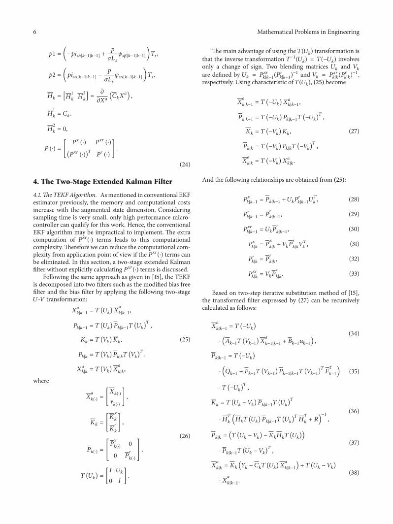
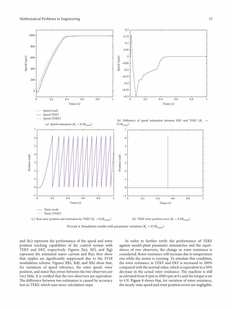