Research Article An Inventory-Theory-Based Inexact...
16
Hindawi Publishing Corporation Mathematical Problems in Engineering Volume 2013, Article ID 482095, 15 pages http://dx.doi.org/10.1155/2013/482095 Research Article An Inventory-Theory-Based Inexact Multistage Stochastic Programming Model for Water Resources Management M. Q. Suo, 1 Y. P. Li, 1 G. H. Huang, 1 Y. R. Fan, 2 and Z. Li 2 1 MOE Key Laboratory of Regional Energy Systems Optimization, Sino-Canada Energy and Environmental Research Academy, North China Electric Power University, Zhuxinzhuang, Beijing 102206, China 2 Faculty of Engineering and Applied Science, University of Regina, Regina, SK, Canada S4S 0A2 Correspondence should be addressed to Y. P. Li; [email protected] Received 31 December 2012; Accepted 1 March 2013 Academic Editor: Xiaosheng Qin Copyright © 2013 M. Q. Suo et al. is is an open access article distributed under the Creative Commons Attribution License, which permits unrestricted use, distribution, and reproduction in any medium, provided the original work is properly cited. An inventory-theory-based inexact multistage stochastic programming (IB-IMSP) method is developed for planning water resources systems under uncertainty. e IB-IMSP is based on inexact multistage stochastic programming and inventory theory. e IB-IMSP cannot only effectively handle system uncertainties represented as probability density functions and discrete intervals but also efficiently reflect dynamic features of system conditions under different flow levels within a multistage context. Moreover, it can provide reasonable transferring schemes (i.e., the amount and batch of transferring as well as the corresponding transferring period) associated with various flow scenarios for solving water shortage problems. e applicability of the proposed IB-IMSP is demonstrated by a case study of planning water resources management. e solutions obtained are helpful for decision makers in not only identifying different transferring schemes when the promised water is not met, but also making decisions of water allocation associated with different economic objectives. 1. Introduction With speedy population growth, the constantly increasing demand for water in terms of both sufficient quantity and satisfied quality has forced a number of researchers to draw optimal water resources management policies [1–5]. However, water resources systems can be complex with uncertainties which may exist in technical, social, environ- mental, political, and financial factors. In addition, these complexities and uncertainties could be multiplied by not only the dynamic characteristics of the system, but also the related economic deficits if the targeted demand is not met. Furthermore, because of the temporal and spatial variations of the relationships between water demand and supply, the desired schemes for water allocation may also vary dynamically [6]. Correspondingly, insufficient water may be encountered particularly in the case of continuously low flow levels over a long period. erefore, it is deemed necessary to develop effective optimization methods for supporting water resources management under such complexities. Previously, numerous methods were developed for plan- ning water resources management systems under various uncertainties [7–12]. Among them, two-stage stochastic pro- gramming (TSP) was an effective technique for problems where an analysis of policy scenarios was desired and the related coefficients are random with known probabil- ity distributions. e fundamental idea behind TSP is the concept of recourse, which is the ability to take corrective actions aſter a random event has taken place [13, 14]. In the past decades, TSP was developed and applied in water resources management under uncertainty [15–21]. However, TSP can only take recourse actions at the second stage to correct any infeasibility, and thus, it can hardly reflect the dynamic variations of system conditions, especially for multistage problems with a sequential structure. To address such a dynamic characteristic, a lot of multistage stochastic programming (MSP) methods were proposed as extensions of dynamic stochastic optimization approaches [13, 22–28]. MSP was improved upon the conventional TSP methods by permitting revised decisions in each time stage based on the information of sequentially realized uncertain events [29]. e uncertain information in an MSP was oſten modeled through a multilayer scenario tree. e primary advantage of
Transcript of Research Article An Inventory-Theory-Based Inexact...

Hindawi Publishing CorporationMathematical Problems in EngineeringVolume 2013 Article ID 482095 15 pageshttpdxdoiorg1011552013482095
Research ArticleAn Inventory-Theory-Based Inexact Multistage StochasticProgramming Model for Water Resources Management
M Q Suo1 Y P Li1 G H Huang1 Y R Fan2 and Z Li2
1 MOE Key Laboratory of Regional Energy Systems Optimization Sino-Canada Energy and Environmental Research AcademyNorth China Electric Power University Zhuxinzhuang Beijing 102206 China
2 Faculty of Engineering and Applied Science University of Regina Regina SK Canada S4S 0A2
Correspondence should be addressed to Y P Li yongpingliiseisorg
Received 31 December 2012 Accepted 1 March 2013
Academic Editor Xiaosheng Qin
Copyright copy 2013 M Q Suo et alThis is an open access article distributed under theCreativeCommonsAttributionLicensewhichpermits unrestricted use distribution and reproduction in any medium provided the original work is properly cited
An inventory-theory-based inexact multistage stochastic programming (IB-IMSP) method is developed for planning waterresources systems under uncertainty The IB-IMSP is based on inexact multistage stochastic programming and inventory theoryThe IB-IMSP cannot only effectively handle system uncertainties represented as probability density functions and discrete intervalsbut also efficiently reflect dynamic features of system conditions under different flow levels within a multistage context Moreoverit can provide reasonable transferring schemes (ie the amount and batch of transferring as well as the corresponding transferringperiod) associated with various flow scenarios for solving water shortage problems The applicability of the proposed IB-IMSP isdemonstrated by a case study of planning water resources management The solutions obtained are helpful for decision makersin not only identifying different transferring schemes when the promised water is not met but also making decisions of waterallocation associated with different economic objectives
1 IntroductionWith speedy population growth the constantly increasingdemand for water in terms of both sufficient quantity andsatisfied quality has forced a number of researchers todraw optimal water resources management policies [1ndash5]However water resources systems can be complex withuncertainties which may exist in technical social environ-mental political and financial factors In addition thesecomplexities and uncertainties could be multiplied by notonly the dynamic characteristics of the system but alsothe related economic deficits if the targeted demand isnot met Furthermore because of the temporal and spatialvariations of the relationships between water demand andsupply the desired schemes for water allocationmay also varydynamically [6] Correspondingly insufficient water may beencountered particularly in the case of continuously low flowlevels over a long periodTherefore it is deemed necessary todevelop effective optimization methods for supporting waterresources management under such complexities
Previously numerous methods were developed for plan-ning water resources management systems under various
uncertainties [7ndash12] Among them two-stage stochastic pro-gramming (TSP) was an effective technique for problemswhere an analysis of policy scenarios was desired andthe related coefficients are random with known probabil-ity distributions The fundamental idea behind TSP is theconcept of recourse which is the ability to take correctiveactions after a random event has taken place [13 14] Inthe past decades TSP was developed and applied in waterresources management under uncertainty [15ndash21] HoweverTSP can only take recourse actions at the second stageto correct any infeasibility and thus it can hardly reflectthe dynamic variations of system conditions especially formultistage problems with a sequential structure To addresssuch a dynamic characteristic a lot of multistage stochasticprogramming (MSP) methods were proposed as extensionsof dynamic stochastic optimization approaches [13 22ndash28]MSP was improved upon the conventional TSP methods bypermitting revised decisions in each time stage based on theinformation of sequentially realized uncertain events [29]The uncertain information in an MSP was often modeledthrough a multilayer scenario tree The primary advantage of
2 Mathematical Problems in Engineering
scenario-based stochastic programming was the flexibility itoffered inmodeling the decision process and defining the sce-narios particularly if the state dimensionwas high [22] A fewresearchers applied the MSP to water resources managementunder uncertainty [24 30ndash32] For example Li and Huang[31] developed a fuzzy-stochastic-based violation analysisapproach for the planning of water resources managementsystems with uncertain information based on a multistagefuzzy-stochastic integer programming model Zhou et al[32] developed a factorial multistage stochastic programmingapproach to obtain the desired water-allocation schemes andmaximize the total net benefit under multiple uncertaintiesAlthough the MSP was useful for dealing with probabilis-tic uncertainties within the optimization framework itsrecourse action was to minimize penalties resulted fromwater shortages not to provide a useful alternative to solvethis problem positively Actually in the case of insufficiencyonly penalties analysis is not enough and more efforts areneeded to solve the insufficiency corresponding to variouspenalties Undoubtedly transferring water from abundantregions would be a preferred choice for the water shortageproblem In this case three questions should be answered bythe managers (a) how much is the amount of transferringwater associated with different flow levels (b) How much isthe transferring batch corresponding to varied transferringamount each time (c) How long is the transferring periodbetween every two transferring actions Fortunately all thesechallenges can bewell responded by the inventory theoryTheaimof the inventory theory is to design schemes formanagersto maximize system benefitminimize system cost as well asguarantee the usersrsquo demand for materials
In the past decades a number of methods based oninventory theory were developed for solving the problems ofmaterialsrsquo supply and demand [33ndash38] For instance Axsater[39] considered a two-echelon distribution inventory systemwith a central warehouse and a number of retailers where thesystem is controlled by continuous review installation stockpolicies with given batch quantities Gupta et al [40] pro-posed a discrete-time model for setting clearance prices forclearing retail inventories of fashion goods where a heuris-tic procedure was developed to find near-optimal pricesYadavalli et al [41] considered a continuous review inventorysystem at a service facility wherein an item demanded by acustomer was issued to himher only after performing serviceof random duration on the item Arnold et al [42] developeda deterministic optimal control approach optimizing theprocurement and inventory policy of an enterprise that isprocessing a rawmaterial when the purchasing price holdingcost and the demand rate are fluctuating over time Schmittet al [43] modeled a retailer whose supplier was subjectto complete supply disruptions where discrete event uncer-tainty and continuous sources of uncertainty were combinedTsao and Lu [44] addressed an integrated facility locationand inventory allocation problem through considering twotypes of transportation cost discounts quantity discountsfor inbound transportation cost and distance discounts foroutbound transportation cost However most of the pastinventory models were rarely developed and applied in waterresources management Although Suo et al [21] proposed an
inventory-theory-based two-stage stochastic programmingmodel for solving water shortage problem this model didnot consider the dynamic variations of system conditionsparticularly for sequential influences of different flow levelsamong multiple stages In addition multiple uncertaintiesexisted in water resources management systems such as thecontinuously changed water availabilities various targetedwater demand associated with timely policy scenarios andfluctuant water benefit as well as related transferring costTheconventional inexact optimizationmethods had difficulties intackling such complexities
Therefore as an extension of the previous efforts aninventory-theory-based inexact multistage stochastic pro-grammingmodel (IB-IMSP)will be developed for supportingwater resources management planning The IB-IMSP is anintegrated method of inventory theory inexact optimiza-tion and multistage stochastic programming It can tackleuncertainties represented as not only probability densityfunctions but also discrete intervals as well as identify thesystem dynamics and decision processes under a series ofscenarios In addition water transferring is exercised withrecourse against any infeasibility which allows exhaustiveanalyses of different policy scenarios with respect to var-ied levels of economic consequences if the targeted waterallocations are infringed Correspondingly reasonable trans-ferring schemes (the transferring amount batch and thecorresponding transferring period) associated with variousflow scenarios would be provided for decision makers forsolving water shortage problem A hypothetical case studyof water resources management will then be provided tovalidate the applicability of the developed approach Theresults obtained can help the managers gain insight intothe water resources management with maximizing economicobjectives and satisfying targeted water demands from users
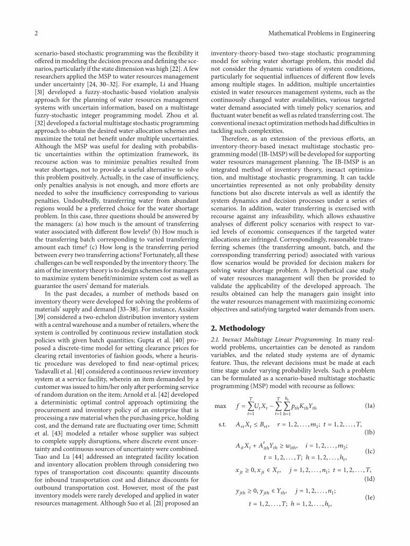
2 Methodology21 Inexact Multistage Linear Programming In many real-world problems uncertainties can be denoted as randomvariables and the related study systems are of dynamicfeature Thus the relevant decisions must be made at eachtime stage under varying probability levels Such a problemcan be formulated as a scenario-based multistage stochasticprogramming (MSP) model with recourse as follows
max 119891 =
119879
sum119905=1
119880119905119883119905minus
119879
sum119905=1
ℎ119905
sumℎ=1
119901119905ℎ119870119905ℎ119884119905ℎ
(1a)
st 119860119903119905119883119905le 119861119903119905 119903 = 1 2 119898
1 119905 = 1 2 119879
(1b)
119860119894119905119883119905+ 1198601015840
119894119905ℎ119884119905ℎge 119908119894119905ℎ 119894 = 1 2 119898
2
119905 = 1 2 119879 ℎ = 1 2 ℎ119905
(1c)
119909119895119905ge 0 119909
119895119905isin 119883119905 119895 = 1 2 119899
1 119905 = 1 2 119879
(1d)
119910119895119905ℎge 0 119910
119895119905ℎisin 119884119905ℎ 119895 = 1 2 119899
1
119905 = 1 2 119879 ℎ = 1 2 ℎ119905
(1e)
Mathematical Problems in Engineering 3
where 119901119905ℎis the probability of occurrence for scenario ℎ in
period 119905 with 119901119905ℎge 0 and sumℎ119905
ℎ=1119901119905ℎ= 1 119870
119905ℎare coefficients
of recourse variables (119884119905ℎ) in the objective function 1198601015840
119894119905ℎare
coefficients of 119884119905ℎin constraint 119894 119908
119894119905ℎis the random variable
of constraint 119894 which is associated with probability levels119902119905ℎ ℎ119905is the number of scenarios in period 119905 with the total
being119867 = sum119879119905=1ℎ119905 In model (1a)ndash(1e) the decision variables
are divided into two subsets those that must be determinedbefore the realizations of random variables are known (ie119909119895119905) and those (recourse variables) that can be determined
after the realized random-variable values are available (ie119910119895119905ℎ)Obviously model (1a)ndash(1e) can only deal with uncertain-
ties in the right-hand sides expressed as PDFs (probabilitydensity functions) when coefficients in 119860 and 119880 are deter-ministic However in real-world problems the quality ofinformation that can be obtained is often not good enough tobe expressed as probabilistic distributions in addition eventhough these distributions are available reflection of them inlarge-scale MSP models could be extremely challenging [45]Correspondingly interval parameters can be introduced intothe multistage programming framework to identify uncer-tainties in parameters This leads to an integrated inexactMSP (IMSP) model as follows
Max 119891plusmn=
119879
sum119905=1
119880plusmn
119905119883plusmn
119905minus
119879
sum119905=1
ℎ119905
sumℎ=1
119901119905ℎ119870plusmn
119905ℎ119884plusmn
119905ℎ(2a)
st 119860plusmn
119903119905119883plusmn
119905le 119861plusmn
119903119905 119903 = 1 2 119898
1
119905 = 1 2 119879(2b)
119860plusmn
119894119905119883plusmn
119905+ 119860plusmn1015840
119894119905ℎ119884plusmn
119905ℎge 119908plusmn
119894119905ℎ 119894 = 1 2 119898
2
119905 = 1 2 119879 ℎ = 1 2 ℎ119905
(2c)
119909plusmn
119895119905ge 0 119909
plusmn
119895119905isin 119883plusmn
119905 119895 = 1 2 119899
1 119905 = 1 2 119879
(2d)
119910plusmn
119895119905ℎge 0 119910
plusmn
119895119905ℎisin 119884plusmn
119905ℎ 119895 = 1 2 119899
1
119905 = 1 2 119879 ℎ = 1 2 ℎ119905
(2e)
where 119880plusmn119905 119883plusmn119905 119870plusmn119905ℎ 119884plusmn119905ℎ 119860plusmn119903119905 119861plusmn119903119905 119860plusmn119894119905 119860plusmn1015840119894119905ℎ and 119908plusmn
119894119905ℎare
interval parametersvariables An interval is defined as anumber with known upper and lower bounds but unknowndistribution information [46] Let 119880minus
119905and 119880+
119905be the lower
and upper bounds of 119880plusmn119905 respectively When 119880minus
119905= 119880+119905 119880plusmn119905
becomes a deterministic numberHowever in water resources management system with
the shortage of water availability water transferring fromother abundant regions is considered as an adaptive measureto meet the water demands in arid regions In this caseit is noticed that the reservoir storage capacity availablewater transferring and the related costs happened in thetransferring process (eg communication cost unit cost andreservoirrsquos protection cost) should be considered In additiontransferring too much water cannot only make the cost of
reservoir operation insurance and protection increase butalso can bring on a high risk for the reservoirrsquos storagecapacity transferring too little water is not enough to satisfythe water demand and can increase the transferring timesHence reasonable transferring batch size and period areneeded to optimize the transferring process which is actuallyan inventory problem Therefore it is necessary to introduceinventory theory into the water resources management sys-tem [21]
22 Inventory-Theory-Based InexactMultistage Stochastic Pro-gramming The aim of inventory theory is to ascertain rulesthat managers can use to minimize the cost (maximize thebenefit) associated with balancing the materialsrsquo supply anddemand for different users Supposing that one materialshould be purchased or produced and its shortage is notallowed the demand is 119863 units per unit time The relativecosts include 119878 (setup cost for ordering one batch ($)) 119862(unit cost for purchasing or producing each unit ($unit))and 119862
1(holding cost per unit per unit of time held in
inventory ($month)) In detail setup cost means all the costsfor ordering one batch to replenish the storage includingthe handling charge communication expenses and travellingexpenses encountered in the ordering process unit cost is thepurchase or produce cost for one unit holding cost representsall the costs associated with the storage of the inventoryuntil it is used including the cost of capital tied up spaceinsurance protection and taxes attributed to storage Theobjective is to determine when and how much to replenishinventory in order to minimize the sum of the produce orpurchase costs per unit time [21] Correspondingly a basicEOQ model can be formulated as follows
119891 (119876) =1198621119876
2+119878119863
119876+ 119862119863 (3a)
where119876 is the purchasing or producing batch in the period of119905 11986211198762 is the holding cost per period 119878119863119876 is the ordering
cost per period 119862119863 is the purchase or produce cost perperiod 119891(119876) is the total cost which is a function of 119876 Bysetting the first derivative of119891(119876) to zero (and noting that thesecond derivative is positive) the economic order quantity(batch) can be obtained as follows
119876lowast= radic
2119878119863
1198621
(3b)
Accordingly the purchasing or producing period 119905can beobtained by the following equation
119905 =119876
119863 (3c)
In this case the total cost 119891(119876) would reach its minimumvalue Model (3a)ndash(3c) is the actual economic order quantity(EOQ) model which can effectively tackle the complexitiesof inventory theory issues associated with purchasing orproducing batch and period Actually the similar inventoryproblems exist in water resources management system For
4 Mathematical Problems in Engineering
example the excessive transferring water could bring on risksfor reservoir capacity and water waste Too short a transfer-ring period could increase the transferring cost and bringon inconvenience in management too long a transferringperiod may not meet the water demand and both of thesecould cause economic losses Consequently a comprehensivemethod including both the advantages of EOQ model andIMSP model is needed which leads to an inventory-theory-based inexact multistage stochastic programming (IB-IMSP)model Concretely IB-IMSP can be formulated as follows
Max 119891plusmn=
119879
sum119905=1
119880plusmn
119905119883plusmn
119905
minus
119879
sum119905=1
ℎ119905
sumℎ=1
119901119905ℎ(1
2119862plusmn
1119905119876plusmn
119905ℎ+ 119862plusmn
119905119863plusmn
119905ℎ+119878plusmn119905119863plusmn119905ℎ
119876plusmn119905ℎ
)
(4a)
st 119860plusmn
119903119905119883plusmn
119905le 119861plusmn
119903119905 119903 = 1 2 119898
1
119905 = 1 2 119879(4b)
119860plusmn
119894119905119883plusmn
119905+ (1198601015840
119894119905ℎ)plusmn
119863plusmn
119905ℎge 119908plusmn
119894119905ℎ 119894 = 1 2 119898
2
119905 = 1 2 119879 ℎ = 1 2 ℎ119905
(4c)
119909plusmn
119895119905ge 0 119909
plusmn
119895119905isin 119883plusmn
119905 119895 = 1 2 119899
1 119905 = 1 2 119879
(4d)
119863plusmn
119905ℎ 119905 = 1 2 119879 ℎ = 1 2 ℎ
119905 (4e)
According to (3b) the batch size can be replaced by afunction of119863 Therefore model (4a)ndash(4e) can be transferredas follows
Max 119891plusmn=
119879
sum119905=1
119880plusmn
119905119883plusmn
119905
minus
119879
sum119905=1
ℎ119905
sumℎ=1
119901119905ℎ(1
2119862plusmn
1119905radic2119878plusmn119905119863plusmn119905ℎ
119862plusmn1119905
+119862plusmn
119905119863plusmn
119905ℎ+ radic
119878plusmn119905119863plusmn119905ℎ119862plusmn1119905
2)
(5a)
st 119860plusmn
119903119905119883plusmn
119905le 119861plusmn
119903119905 119903 = 1 2 119898
1
119905 = 1 2 119879(5b)
119860plusmn
119894119905119883plusmn
119905+ (1198601015840
119894119905ℎ)plusmn
119863plusmn
119905ℎge 119908plusmn
119894119905ℎ 119894 = 1 2 119898
2
119905 = 1 2 119879 ℎ = 1 2 ℎ119905
(5c)
119909plusmn
119895119905ge 0 119909
plusmn
119895119905isin 119883plusmn
119905 119895 = 1 2 119899
1 119905 = 1 2 119879
(5d)
119863plusmn
119905ℎ 119905 = 1 2 119879 ℎ = 1 2 ℎ
119905 (5e)
119876plusmn
119905ℎ= radic
2119878plusmn119905119863plusmn119905ℎ
119862plusmn1119905
(5f)
In (5a) let119891plusmn = 119891plusmn1minus119891plusmn2 in which119891plusmn
1= sum119879
119905=1119880plusmn119905119883plusmn119905 and119891plusmn
2=
sum119879
119905=sumℎ119905
ℎ=1119901119905ℎ(12119862plusmn
1119905radic2119878plusmn119905119863plusmn119905ℎ119862plusmn1119905+ 119862plusmn119905119863plusmn119905ℎ+ radic119878plusmn119905119863plusmn119905ℎ119862plusmn11199052)
Since119862plusmn1119905 119878plusmn119905 and119862plusmn
119905are parameters about different costs and
119863plusmn119905ℎis variable about transferring water all of them would be
greater than zero In addition 119901119905ℎis probability and thus it
can be easily obtained that 119891plusmn2ge 0 and 119891plusmn
2is an increasing
function of 119862plusmn1119905 119878plusmn119905 119862plusmn119905 and119863plusmn
119905ℎ In this case |119891
2|minusSign(119891minus
2) =
119891minus
2and |119891
2|+Sign(119891+
2) = 119891
+
2 Accordingly model (5a)ndash(5f)
can be converted into two deterministic submodels based ona two-step interactive algorithm [47] The submodel for 119891+can be formulated in the first step when the system objectiveis to be maximized the other submodel (corresponding to119891minus) can then be formulated based on the solution of the first
submodel Therefore the first submodel is
Max 119891+=
119879
sum119905=1
(
1198951
sum119895=1
119906+
119895119905119909+
119895119905+
1198991
sum119895=1198951+1
119906+
119895119905119909minus
119895119905)
minus
119879
sum119905=1
ℎ119905
sumℎ=1
119901119905ℎ(1
2119862minus
1119905radic2119878minus119905119863minus119905ℎ
119862minus1119905
+119862minus
119905119863minus
119905ℎ+ radic
119878minus119905119863minus119905ℎ119862minus1119905
2)
(6a)
st1198951
sum119895=1
10038161003816100381610038161003816119886119903119895119905
10038161003816100381610038161003816
minus
sign (119886minus119903119895119905) 119909+
119895119905
+
1198991
sum119895=1198951+1
10038161003816100381610038161003816119886119903119895119905
10038161003816100381610038161003816
+
sign (119886+119903119895119905) 119909minus
119895119905le 119861+
119903119905
119903 = 1 2 1198981 119905 = 1 2 119879
(6b)
1198951
sum119895=1
10038161003816100381610038161003816119886119894119895119905
10038161003816100381610038161003816
minus
sign (119886minus119894119895119905) 119909+
119895119905+
1198991
sum119895=1198951+1
10038161003816100381610038161003816119886119894119895119905
10038161003816100381610038161003816
+
sign (119886+119894119895119905) 119909minus
119895119905
+100381610038161003816100381610038161198601015840
119894119905ℎ
10038161003816100381610038161003816
+
sign (1198601015840+119894119905ℎ)119863minus
119905ℎge 119908minus
119894119905ℎ
119894 = 1 2 1198982 119905 = 1 2 119879 ℎ = 1 2 ℎ
119905
(6c)
119909+
119895119905ge 0 119895 = 1 2 119895
1 119905 = 1 2 119879 (6d)
119909minus
119895119905ge 0 119895 = 119895
1+ 1 1198951+ 2 119899
1 119905 = 1 2 119879
(6e)
119863minus
119905ℎ 119905 = 1 2 119879 ℎ = 1 2 ℎ
119905 (6f)
119876minus
119905ℎ= radic
2119878minus119905119863minus119905ℎ
119862minus1119905
(6g)
where 119909plusmn119895119905(119895 = 1 2 119895
1) are interval variables with positive
coefficients in the objective function 119909plusmn119895119905
(119895 = 1198951+ 1 1198951+
2 1198991) are interval variables with negative coefficients
Solutions of 119909+119895119905 opt (119895 = 1 2 1198951) 119909
minus
119895119905 opt (119895 = 1198951 + 1 1198951 +
Mathematical Problems in Engineering 5
2 1198991)119863minus119905ℎ opt and119876
minus
119905ℎ opt can be obtained from submodel(6a)ndash(6g) Based on the above solutions the second submodelfor 119891minus can be formulated as follows
Max 119891minus=
119879
sum119905=1
(
1198951
sum119895=1
119906minus
119895119905119909minus
119895119905+
1198991
sum119895=1198951+1
119906minus
119895119905119909+
119895119905)
minus
119879
sum119905=1
ℎ119905
sumℎ=1
119901119905ℎ(1
2119862+
1119905radic2119878+119905119863+119905ℎ
119862+1119905
+119862+
119905119863+
119905ℎ+ radic
119878+119905119863+119905ℎ119862+1119905
2)
(7a)
st1198951
sum119895=1
10038161003816100381610038161003816119886119903119895119905
10038161003816100381610038161003816
+
119904ign (119886+119903119895119905) 119909minus
119895119905
+
1198991
sum119895=1198951+1
10038161003816100381610038161003816119886119903119895119905
10038161003816100381610038161003816
minus
sign (119886minus119903119895119905) 119909+
119895119905le 119861minus
119903119905
119903 = 1 2 1198981 119905 = 1 2 119879
(7b)
1198951
sum119895=1
10038161003816100381610038161003816119886119894119895119905
10038161003816100381610038161003816
+
sign (119886+119894119895119905) 119909minus
119895119905+
1198991
sum119895=1198951+1
10038161003816100381610038161003816119886119894119895119905
10038161003816100381610038161003816
minus
sign (119886minus119894119895119905) 119909+
119895119905
+100381610038161003816100381610038161198601015840
119894119905ℎ
10038161003816100381610038161003816
minus
sign (1198601015840minus119894119905ℎ)119863+
119905ℎge 119908+
119894119905ℎ
119894 = 1 2 1198982 119905 = 1 2 119879 ℎ = 1 2 ℎ
119905
(7c)
0 le 119909minus
119895119905le 119909+
119895119905 opt 119895 = 1 2 1198951 119905 = 1 2 119879
(7d)
119909+
119895119905ge 119909minus
119895119905 opt 119895 = 1198951 + 1 1198951 + 2 1198991 119905 = 1 2 119879
(7e)
119863minus
119905ℎle 119863+
119905ℎ opt 119905 = 1 2 119879 ℎ = 1 2 ℎ119905
(7f)
119876+
119905ℎ= radic
2119878+119905119863+119905ℎ
119862+1119905
(7g)
Solutions of 119909minus119895119905 opt (119895 = 1 2 1198951) 119909
+
119895119905 opt (119895 = 1198951 + 1 1198951 +2 119899
1) 119863+119905ℎ opt and 119876
+
119905ℎ opt can be obtained by solvingsubmodel (7a)ndash(7g) Then the expected objective functionvalue can be calculated as follows
119891+
opt =119879
sum119905=1
(
1198951
sum119895=1
119906+
119895119905119909+
119895119905+
1198991
sum119895=1198951+1
119906+
119895119905119909minus
119895119905)
minus
119879
sum119905=1
ℎ119905
sumℎ=1
119901119905ℎ(1
2119862minus
1119905radic2119878minus119905119863minus119905ℎ
119862minus1119905
+119862minus
119905119863minus
119905ℎ+ radic
119878minus
119905119863minus
119905ℎ119862minus
1119905
2)
(8a)
119891minus
opt =119879
sum119905=1
(
1198951
sum119895=1
119906minus
119895119905119909minus
119895119905+
1198991
sum119895=1198951+1
119906minus
119895119905119909+
119895119905)
minus
119879
sum119905=1
ℎ119905
sumℎ=1
119901119905ℎ(1
2119862+
1119905radic2119878+119905119863+119905ℎ
119862+1119905
+119862+
119905119863+
119905ℎ+ radic
119878+119905119863+119905ℎ119862+1119905
2)
(8b)
Consequently through combining solutions of submodels(6a)ndash(6g) and (7a)ndash(7g) the solution for IB-IMSP model canbe obtained as follows
119909plusmn
119895119905 opt = [119909minus
119895119905 opt 119909+
119895119905 opt] forall119895 119905 (8c)
119863plusmn
119905ℎ opt = [119863minus
119905ℎ opt 119863+
119905ℎ opt] forall119905 ℎ = 1 2 ℎ119905 (8d)
119876plusmn
119905ℎ opt = [119876minus
119905ℎ opt 119876+
119905ℎ opt] forall119905 ℎ = 1 2 ℎ119905 (8e)
119891plusmn
opt = [119891minus
opt 119891+
opt] (8f)
Figure 1 shows the framework of the IB-IMSP model whichis based on EOQ and IMSP techniques The introduction ofEOQmodel makes the IB-IMSP can provide the transferringbatch size and period avoiding unnecessary waste of capitaland time as well as solving water shortage problem Theapplication of IMSP enhances the IB-IMSPrsquos capacities inhandling the uncertainties and dynamic complexities Forexample the proposed IB-IMSP can tackle uncertaintiesexpressed as random variables interval parameters as wellas their combinations In addition the IB-IMSP can identifydynamics of not only the uncertainties but also the relateddecisions Therefore the method can be used for generatingdecision alternatives and help decision makers to identifydesired policies under different flow levels and analyze allpossible policy scenarios that are associated with differenttransferring schemes
3 Application
The following water resources management problem will beused to demonstrate the applicability of the proposed IB-IMSP model A manager is responsible for delivering waterfrom an unregulated reservoir during three planning periods(with each one being five years) to three users a municipalityan industrial concern and an agricultural sector All userswant to know howmuch water they can expect over the threeperiods If the promised water is delivered a net benefit tothe local economy will be generated for each unit of waterallocated However if the promised water is not deliveredthey will try to transfer water from other abundant watersources to ensure the local normal life and economic growthCorrespondingly transferring water will be decided based onthe available water resources and target demands from thethree users In addition although transferringwater can solvethe water shortage problem it will result in a reduced netsystem benefit from three main aspects setup cost unit cost
6 Mathematical Problems in Engineering
Dynamic policy analysis
Uncertainties Inventory phenomenon
Multistage stochastic programming (MSP)
Probabilistic distributions
Discrete intervals
Interval programming (ILP)
Inventory theory
EOQ modelInterval-parameter multistage
stochastic programming (IMSP)
Inventory-theory-based inexact multistage stochastic programming (IB-IMSP)
Optimal solutions
Generation of decision alternatives
Submodel (1) for119891+ Submodel (2) for 119891minus
Figure 1 Framework of the IB-IMSP model
Table 1 Stream flows in the three periods (supply)
Stream flowlevel Probability Stream flow (106 m3)
119905 = 1 119905 = 2 119905 = 3
Low (L) 02 [42 58] [47 65] [43 59]
Medium (M) 06 [80 96] [79 89] [83 92]
High (H) 02 [123 136] [118 139] [126 134]
Table 2 Water allocation targets for users
Time period119905 = 1 119905 = 2 119905 = 3
Water allocation target (106 m3)119882plusmn
1119905(to municipal) [41 51] [55 64] [64 75]
119882plusmn
2119905(to industrial) 62 [72 83] [78 89]
119882plusmn3119905(to agricultural) 78 91 [87 91]
Maximum allowable allocation(106 m3)119882plusmn1119905 max (to municipal) [41 45] [54 60] [54 61]
119882plusmn2119905 max (to industrial) [51 55] [68 74] [72 94]
119882plusmn
3119905 max (to agricultural) [65 83] [70 81] [73 81]
and holding cost for water transferring Tables 1 and 2 denotethe available water resources from the local region and targetdemands Table 3 provides the associated economic dataTheobjective is tomaximize the expected value of the net benefitsover the planning horizon
Under this condition random variables (available watersupply) with probability 119901
119905ℎto construct three scenario trees
for the planning horizon with a branching structure of 1-3-3-3 can be applied Therefore a three-period (four-stage)scenario tree can be generated for each of the three water
Table 3 Related economic data
Time period119905 = 1 119905 = 2 119905 = 3
Net benefit when waterdemand is satisfied NBplusmn
119894119905
($m3)Municipal (119894 = 1) [90 110] [95 115] [100 120]
Industrial (119894 = 2) [45 55] [55 70] [65 85]
Agricultural (119894 = 3) [30 35] [35 50] [35 50]
Costs when water istransferred119862plusmn
1119905(holding cost $m3) [180 220] [190 230] [200 250]
119862plusmn119905(unit cost $m3) [12 16] [23 30] [34 40]
119878plusmn119905(setup cost $) [65 80] [70 90] [75 90]
users All of the scenario trees have the same structure withone initial node at time 0 and three succeeding ones in period1 each node in period 1 has three succeeding nodes in period2 and so on for each node in period 3These result in 27 nodesin period 3 (and thus 81 scenarios since here are three waterusers) Figure 2 shows the formulation of the scenario tree
In this study the random streamflowunder each scenariomay be expressed as discrete interval Moreover the relevantwater allocation plan would be of dynamic feature wherethe related decisions must be made at discrete points intime under multiple probability levels In addition differenttransferring water under each probability level will affect thesystem benefit For example if too much water is transferredper unit time the holding cost will increase conversely iftoo little water is transferred per unit time the transferringfrequency and setup cost will increase Therefore to identifythese uncertainties and dynamics as well as solving the water
Mathematical Problems in Engineering 7
Reservoir
Period 1
Period 2
Period 3
MunicipalIndustrialAgricultural
L
MHL
MH
L
M
HLMH L
MH
119864plusmn327
119864plusmn29
119864plusmn13
119864plusmn31
119864plusmn21
119864plusmn11119901plusmn119905ℎ
Figure 2 Formulation of scenario tree
shortage problem an IB-IMSP model can be formulated asfollows
Max 119891plusmn=
119868
sum119894=1
119879
sum119905=1
119873119861plusmn
119894119905119882plusmn
119894119905
minus
119879
sum119905=1
ℎ119905
sumℎ=1
119901119905ℎ(1
2119862plusmn
1119905radic2119878plusmn119905119863+119905ℎ
119862plusmn1119905
+119862plusmn
119905119863plusmn
119905ℎ+ radic
119878plusmn119905119863plusmn119905ℎ119862plusmn1119905
2)
(9a)
Subject to(constraint of available water flow)119868
sum119894=1
119882plusmn
119894119905
le 119902plusmn
119905ℎ+ 119863plusmn
119905ℎ+ 119864plusmn
(119905minus1)ℎ forall119905 = 1 2 3 ℎ = 1 2 ℎ
119905
(9b)
119902plusmn
119905ℎ+ 119863plusmn
119905ℎ+ 119864plusmn
(119905minus1)ℎ
le
119868
sum119894=1
119882plusmn
119894119905 max forall119905 = 1 2 3 ℎ = 1 2 ℎ119905
(9c)
(constraint of surplus water)
119864plusmn
119905ℎ= 119902plusmn
119905119896+ 119863plusmn
119905ℎminus
119868
sum119894=1
119882plusmn
119894119905
+ 119864plusmn
(119905minus1)ℎ 119864plusmn
0ℎ= 0 forall119905 = 1 2 3 ℎ = 1 2 ℎ
119905
(9d)
(constraint of reservoir capacity)
119902plusmn
119905ℎ+ 119864plusmn
(119905minus1)ℎ+ 119863plusmn
119905ℎminus
119868
sum119894=1
119882plusmn
119894119905le 119877119862plusmn forall119905 ℎ = 1 2 ℎ
119905
(9e)
(constraint of transferring water batch)
119876plusmn
119905ℎ= radic
2119878plusmn119905119863plusmn119905ℎ
119862plusmn1119905
(9f)
(non-negative constraint)
119863plusmn
119905ℎge 0 forall119905 ℎ = 1 2 ℎ
119905 (9g)
where
119894 = water user 119894 = 1 2 3119905 = planning time period 119905 = 1 2 3ℎ = available flow level ℎ = 1 2 ℎ
119905
119901119905ℎ=probability level of available water during period
119905 with 119901119905ℎgt 0 and sumℎ119905
ℎ=1119901119905ℎ= 1
119902plusmn119905ℎ
= random variable of total water availabilityduring period 119905 with probability level of 119901
119905ℎ(m3)
119891plusmn = net system benefit over the planning horizon ($)119862plusmn119905= unit cost for transferring water during period 119905
($m3)119862plusmn1119905= holding cost per unit per unit of time held in
reservoir ($m3)119863plusmn119905ℎ= transferringwater amount fromother abundant
water sources when the total water-allocation target isnot met under the flow of 119902plusmn
119905ℎ(m3)
119864plusmn(119905minus1)ℎ
= surplus flow when water is delivered inperiod 119905 minus 1 (m3)119864plusmn(119905minus2)ℎ
= surplus flow when water is delivered inperiod 119905 minus 2 (m3)119876plusmn119905ℎ
= transferring water batch when the flow is 119902plusmn119905ℎ
(m3)119878plusmn119905= setup cost for transferring one batch ($)
NBplusmn119894119905=net benefit (ie revenueminus expense) to user
119894 per unit of water allocated during period 119905 ($m3)119877119862plusmn = storage capacity of the reservoir (m3)119882plusmn119894119905= fixed allocation target for water that is promised
to user 119894 during period 119905 (m3)119882plusmn119894119905max= maximum amount that should be allocated
to user 119894 during period 119905 (m3)
In model (9a)ndash(9g) 119863plusmn119905ℎ
are decision variables whichare affected by local flow levels Random variables (availablewater supplies) under different probability levels (119901
119905ℎ) are
used to construct the scenario tree Correspondingly theIB-IMSP model can identify nonanticipativity of the water
8 Mathematical Problems in Engineering
Table 4 Solution of the IB-IMSP model (period 1)
Water flow level Probability Optimized transferringwater (106 m3)
Optimized transferringbatch (103 m3)
Optimized transferringperiod (hour)
L 02 [1330 1390] [310 318] [988 1006]
M 06 [950 1010] [262 271] [1159 1191]
H 02 [550 580] [199 205] [1530 1565]
Table 5 Solution of the IB-IMSP model (period 2)
Water flow level Probability Joint flow Optimized transferringwater (106 m3)
Optimized transferringbatch (103 m3)
Optimized transferringperiod (hour)
L 004 L-L [1150 1290] [291 318] [1064 1094]
L 012 L-M [910 970] [259 276] [1227 1229]
L 004 L-H [410 580] [174 213] [1587 1831]
M 012 M-L [770 910] [238 267] [1267 1336]
M 036 M-M [530 590] [198 215] [1573 1611]
M 012 M-H [030 200] [047 125] [2702 6770]
H 004 H-L [370 480] [[165 194] [1744 1928]
H 012 H-M [130 160] [098 112] [3021 3252]
H 004 H-H 0 0 0
resources management system where a decision must bemade in each stage without the knowledge of the realizationsof randomvariables in the future stages Based on themethoddepicted in Section 2 the IB-IMSP model can be convertedinto two deterministic submodels Interval solutions can thenbe obtained by solving the two submodels sequentially Thespecific solution process can be summarized as follows
Step 1 Formulate IB-IMSP model (9a)ndash(9g)
Step 2 Transform model (9a)ndash(9g) into two submodelswhere the upper bound (119891+) is first solved because theobjective is to maximize 119891plusmn
Step 3 Solve the119891+ submodel and obtain solutions of119863minus119905ℎ opt
119876minus119905ℎ opt and 119891
+
opt
Step 4 Formulate the objective function and relevant con-straints of the 119891minus submodel
Step 5 Solve the119891minus submodel and obtain solutions of119863+119905ℎ opt
119876+119905ℎ opt and 119891
minus
opt
Step 6 Make the second programming using ILP basedon the solution of 119863plusmn
119905ℎ opt and obtain the actual allocation119882plusmn119894119905ℎ opt
Step 7 Integrate solutions of the two submodels and119882plusmn119894119905ℎ opt
and the optimal results can be expressed as 119863plusmn119905ℎ opt =
[119863minus119905ℎ opt 119863
+
119905ℎ opt] 119876plusmn
119905ℎ opt = [119876minus119905ℎ opt 119876
+
119905ℎ opt] 119882plusmn
119894119905ℎ opt =
[119882minus119894119905ℎ opt119882
+
119894119905ℎ opt] and 119891plusmn
opt = [119891minus
opt 119891+
opt]
Step 8 Stop
4 Results Analysis
Tables 4ndash6 denote the optimized transferring water schemesunder different flow levels during the planning horizon Itis shown that the solutions for the objective function valueand most of the nonzero decision variables are intervalsCommonly solutions expressed as intervals indicate that theassociated decisions should be sensitive to the uncertainmodeling inputs For instance the interval solutions for 119863plusmn
119905ℎ
under the given targets reveal potential system-conditionvariations caused by uncertain inputs of 119873119861plusmn
119894119905 119862plusmn119905 119862plusmn1119905
119878plusmn119905 and 119902plusmn
119905ℎ The demands and shortages are associated to
water availability Shortages would happen if the availablewater resources cannot satisfy the usersrsquo demands Underthe condition of insufficient water more water needs to betransferred from other abundant water sources to guaranteethe local normal life and economic development
Tables 4ndash6 show the solution of water transferringschemes obtained from the IB-IMSP model including trans-ferring amount transferring batch and transferring periodDifferent transferring water is associated with varied flowlevels and the targeted water demands If the manageris optimistic of water supply to users and thus promisesan upper-bound water quantity the shortages probabilitywould be small and thus less water should be transferredconversely if themanager has a conservative attitude towardswater supply more water should be transferred to meetthe usersrsquo basic demands The transferring batch means thequantity of transferring water in every transferring schemewhich is mainly influenced by the transferring amountThe transferring period represents a cycle length from onethe transferring scheme to the next scheme and equals totransferring batch divided by demand and thenmultiplied byeach planning period
Mathematical Problems in Engineering 9
Table 6 Solution of the IB-IMSP model (period 3)
Water flow level Probability Joint flow Optimized transferringwater (106 m3)
Optimized transferringbatch (103 m3)
Optimized transferringperiod (hour)
L 0008 L-L-L [730 970] [240 264] [1177 1385]
L 0024 L-L-M [400 570] [173 202] [1535 1871]
L 0008 L-L-H [0 140] [0 103] [0 3098]
L 0024 L-M-L [490 650] [192 216] [1438 1690]
L 0072 L-M-M [160 250] [110 134] [2318 2958]
L 0024 L-M-H 0 0 0
L 0008 L-H-L [0 260] [0 137] [0 2273]
L 0024 L-H-M 0 0 0
L 0008 L-H-H 0 0 0
M 0024 M-L-L [350 590] [162 206] [1509 2000]
M 0072 M-L-M [020 190] [039 117] [2659 8366]
M 0024 M-L-H 0 0 0
M 0072 M-M-L [110 270] [091 139] [2417 2789]
M 0216 M-M-M 0 0 0
M 0072 M-M-H 0 0 0
M 0024 M-H-L 0 0 0
M 0072 M-H-M 0 0 0
M 0024 M-H-H 0 0 0
H 0008 H-L-L [0 160] [0 107] [0 2898]
H 0024 H-L-M 0 0 0
H 0008 H-L-H 0 0 0
H 0024 H-M-L 0 0 0
H 0072 H-M-M 0 0 0
H 0024 H-M-H 0 0 0
H 0008 H-H-L 0 0 0
H 0024 H-H-M 0 0 0
H 0008 H-H-H 0 0 0
Total expected value of net benefit ($109) 119891plusmnopt = [353 503]
Table 4 provides the optimized water transferringschemes under three different flow levels in the first periodFor example the solutions of119863plusmn
11 opt = [1330 1390]times 106m3
means much more water should be transferred under lowflow level (probability = 20) which leads to larger transf-erring batch (119876plusmn
11 opt = [310 318] times 103m3) Corresp-ondingly the transferring period ([988 1006] hour) wouldbe smaller which is calculated by (3c) and means that thetransferring frequency would become more frequent Whenthe flow level is medium (probability = 60) the transferringwater (119863plusmn
12 opt = [950 1010] times 106m3) and transferringbatch (119876plusmn
12 opt = [262 271] times 103m3) are smaller thanthe solutions of low flow level which are associated witha wide transferring period ([1159 1191] hour) Underhigh flow level (probability = 20) the related transferringwater and transferring batch are the smallest while thetransferring period is the widest being [550 580] times 106m3[199 205] times 103m3 and [1530 1565] hour individually
This implies that the water shortage under high flow is theleast serious compared with low and medium flow levelsunder the same demand condition
Table 5 presents the optimized water transferringschemes under all possible scenarios in period 2 Under low-medium- high-flow levels in period 2 (following a lowflow in period 1) the needing transferring water would be[1150 1290] times 10
6m3 [910 970] times 106m3 and[410 580] times 106m3 respectively (with probability levelsof 4 12 and 4) Accordingly the transferring batcheswould be [291 318] times 103m3 [259 276] times 103m3 and[174 213] times 103m3 individually associated with thetransferring periods being [1064 1094] hour [1227 1229]hour and [1587 1831] hour This transferring schemedemonstrates that although the water flow is high inperiod 2 water transferring is still needed since lowflow is in period 1 On the contrast the solutions of119863plusmn
27 opt = [370 480]times106m3119863plusmn
28 opt = [130 160]times106m3
10 Mathematical Problems in Engineering
01234567
L M HWater flow level
Lower boundUpper bound
119894 = 1 119894 = 2 119894 = 3 119894 = 1 119894 = 2 119894 = 3 119894 = 1 119894 = 2 119894 = 3
Opt
imiz
ed w
ater
allo
catio
n (106m3)
(a)
0123456
87
L M HWater flow level
Lower boundUpper bound
119894 = 1 119894 = 2 119894 = 3 119894 = 1 119894 = 2 119894 = 3 119894 = 1 119894 = 2 119894 = 3
Opt
imiz
ed w
ater
allo
catio
n (106m3)
(b)
Figure 3 (a) Optimized water allocation from local water source in period 1 (b) Optimized water allocation from water transferring inperiod 1
and119863plusmn29 opt = 0 imply that there would be less water shortages
even without shortages during the second period if the waterflow is high in the first period
Table 6 shows the optimized water transferring alterna-tives under all possible scenarios in period 3The solutions of119863plusmn
31 opt = [730 970] times 106m3119863plusmn
32 opt = [400 570] times 106m3
and 119863plusmn33 opt = [0 140] times 10
6m3 mean that if the flows arelow in the previous two periods there would be [730 970]times106m3 [400 570]times106m3 and [0 140]times106m3 of transfer-ring water under lowmedium and highwater-flow scenariosindividually (probability = 08 24 and 08) followedwith the transferring batch being [240 264] times 103m3[173 202]times103m3 and [0 103]times103m3 individually If theflow is low in period 1 and high in period 2 then there wouldbe [0 260] times 106m3 0 and 0 of water transferring neededunder low- medium- and high-flow scenarios in period 3The water shortage in period 3 would become less if there issome surplus in the reservoir due to the high-flow conditionduring period 2
The solutions also indicate that under the worst-casescenario (probability = 08) when the water flows are lowduring the entire planning period the total of transferringwater would be [730 970] times 106m3 associated with the totalwater demand from the three users being [229 255]times106m3implying a serious shortage in water supply Therefore theusers need to transfer water from the other more expensivesources and ensure their demands Under the best scenario(probability = 08) when the water flows are high duringthe entire planning period the total of transferring waterwould be 0 indicating that the water demands of the threeusers could generally be satisfied Although the probability ofthe worst-case scenario is low (08) the deficits due to theoccurrence of such an extreme event are high Consequentlyan optimal policy that is formulated based on the analyses ofnot only the system benefits but also the related deficits wouldbe desired
Two extreme expected values of the net system benefitover the planning period are provided by the solution of
the objective function (119891plusmnopt = $ [353 503] times 109) With theactual value of every continuous variable changing withinits lower and upper bounds the desired system benefitwould fluctuate accordingly between 119891minusopt and 119891+opt witha range of dependability levels Given varied water avail-ability conditions and underlying probability distributionsthe consequential plans of water transferring (and systembenefit) would differ between their related solution intervalsA plan with lower system benefit might need more watertransferring while that of higher benefitwould link to smallertransferring water under advantageous situations
With water transferring usersrsquo demands can be wellsatisfied under various water flow levels and meanwhilewater shortage risks can be avoided Figures 3ndash6 show theoptimized water allocations from the local water source andthe transferring under different flow levels over the planninghorizon (except the optimized water allocation from H-L-Lto H-H-H in period 3) With only considering local wateravailability the allotment to the agricultural sector wouldbe first decreased followed by that to industrial sector inthe case of water insufficiency The municipal use wouldbe guaranteed because it brings the highest benefit whenits water demand is met In comparison the industrial andagricultural uses match to lower benefits (see Table 3)
Figures 3(a) and 3(b) describe the optimized waterallocations to three users from the local water source andthe transferring under three flow levels in the first periodrespectively Under low flow the solution of water allocationto municipal sector industrial sector and agricultural sectorwould be [22 38] times 106m3 1 times 106m3 and 1 times 106m3from local water source which implies that encounteringwater shortage the industrial sector and agricultural sectoronly obtain the minimum amount to guarantee their nec-essary uses while the municipal sector can gain more water(Figure 3(a)) Correspondingly the water allocation fromthe transferring to agricultural sector would be the largest(68 times 106m3) followed by industrial sector (52 times 106m3)and municipal sector ([13 19] times 106m3) which are shown
Mathematical Problems in Engineering 11
0
1
2
3
4
5
6
7
8
9
10
L-L L-M L-H M-L M-M M-H H-L H-M H-HWater flow level
Lower boundUpper bound
Opt
imiz
ed w
ater
allo
catio
n (106m3)
119894 = 1 119894 = 2 119894 = 3 119894 = 1 119894 = 2 119894 = 3 119894 = 1 119894 = 2 119894 = 3 119894 = 1 119894 = 2 119894 = 3 119894 = 1 119894 = 2 119894 = 3 119894 = 1 119894 = 2 119894 = 3 119894 = 1 119894 = 2 119894 = 3 119894 = 1 119894 = 2 119894 = 3 119894 = 1 119894 = 2 119894 = 3
(a)
0
1
2
3
4
5
6
7
8
9
L-L L-M L-H M-L M-M M-H H-L H-M H-HWater flow level
Lower boundUpper bound
Opt
imiz
ed w
ater
allo
catio
n (106m3)
119894 = 1 119894 = 2 119894 = 3 119894 = 1 119894 = 2 119894 = 3 119894 = 1 119894 = 2 119894 = 3 119894 = 1 119894 = 2 119894 = 3 119894 = 1 119894 = 2 119894 = 3 119894 = 1 119894 = 2 119894 = 3 119894 = 1 119894 = 2 119894 = 3 119894 = 1 119894 = 2 119894 = 3 119894 = 1 119894 = 2 119894 = 3
(b)
Figure 4 (a) Optimized water allocation from local water source in period 2 (b) Optimized water allocation from water transferring inperiod 2
in Figure 3(b) Under high flow both the targeted waterdemands frommunicipal and industrial users can be satisfiedunder the local water supply while the agricultural sector stillneeds water transferring to reach its targeted demand
Figures 4(a) and 4(b) present the optimized water allo-cations to all users from the local water source and thetransferring under all possible flow scenarios in period 2individually Under low medium and high flow levels inperiod 2 (following a low flow in period 1) the solutionof water allocation to agricultural sector would be 10 times106m3 10 times 106m3 and [33 50] times 106m3 from the local
water supply respectively (with probability levels of 4
12 and 4) correspondingly it would be 81 times 106m381 times 106m3 and [41 58] times 106m3 from transferringindividually This allocation implies that although the waterflow is high in period 2 the agricultural sector still cannotbe satisfied by local water supply since low flow in period1 In comparison the water allocation of [43 54] times 106m3[75 78] times 106m3 and 91 times 106m3 from local water supplyand [37 48] times 106m3 [13 16] times 106m3 and 0 fromtransferring to agricultural sector under the last three flowscenarios implies that lesswater transferringwould be neededduring the second period if the water flow is high in the firstperiod
12 Mathematical Problems in Engineering
0123456789
10
Water flow level
Lower boundUpper bound
Opt
imiz
ed w
ater
allo
catio
n (106m3)
119894 = 1 119894 = 2 119894 = 3 119894 = 1 119894 = 2 119894 = 3 119894 = 1 119894 = 2 119894 = 3 119894 = 1 119894 = 2 119894 = 3 119894 = 1 119894 = 2 119894 = 3 119894 = 1 119894 = 2 119894 = 3 119894 = 1 119894 = 2 119894 = 3 119894 = 1 119894 = 2 119894 = 3 119894 = 1 119894 = 2 119894 = 3
L-L-L L-L-M L-L-H L-M-L L-M-M L-M-H L-H-L L-H-M L-H-H
(a)
0
1
2
3
4
5
6
7
8
9
Water flow level
Lower boundUpper bound
Opt
imiz
ed w
ater
allo
catio
n (106m3)
119894 = 1 119894 = 2 119894 = 3 119894 = 1 119894 = 2 119894 = 3 119894 = 1 119894 = 2 119894 = 3 119894 = 1 119894 = 2 119894 = 3 119894 = 1 119894 = 2 119894 = 3 119894 = 1 119894 = 2 119894 = 3 119894 = 1 119894 = 2 119894 = 3 119894 = 1 119894 = 2 119894 = 3 119894 = 1 119894 = 2 119894 = 3
L-L-L L-L-M L-L-H L-M-L L-M-M L-M-H L-H-L L-H-M L-H-H
(b)
Figure 5 (a) Optimized water allocation from local water source (from L-L-L to L-H-H) in period 3 (b) Optimized water allocation fromwater transferring (from L-L-L to L-H-H) in period 3
Figures 5(a) 5(b) 6(a) and 6(b) provide the optimizedwater allocations to the three users from local water sourceand the transferring under the flow scenarios from L-L-Lto M-H-H in period 3 respectively The water allocation tothe agricultural sector from local water source ([10 18] times106m3 [30 51] times 106m3 and [73 91] times 106m3) under
the scenarios of low-low-low low-low-medium and low-low-high mean that if the flows are low in the previous twoperiods there would be [73 77]times106m3 [40 57]times106m3and [0 14]times106m3 of transferringwater under lowmediumand high water-flow scenarios respectively (probability =08 24 and 08) If the flow is low in period 1 andhigh in period 2 then the water allocation to agricultural
sector would be [61 91] times 106m3 [87 91] times 106m3 and[87 91] times 106m3 from local water source and [0 26] times106m3 0 and 0 from transferring under low- medium- andhigh-flow scenarios in period 3 The water transferring inperiod 3 would be less in the case of some surplus existingowing to the high-flow condition in period 2 Under the flowlevels ofH-L-L toH-H-H the availablewater from localwatersource can basically satisfy the usersrsquo demands and thus alittle of water needs to be transferred which can be seen inTable 3
Based on the above analysis it can be obtained that theIB-IMSP has three main advantages Firstly it can handleuncertainties existing in water flows by producing scenarios
Mathematical Problems in Engineering 13
0123456789
10
Water flow level
Lower boundUpper bound
Opt
imiz
ed w
ater
allo
catio
n (106m3)
119894 = 1 119894 = 2 119894 = 3 119894 = 1 119894 = 2 119894 = 3 119894 = 1 119894 = 2 119894 = 3 119894 = 1 119894 = 2 119894 = 3 119894 = 1 119894 = 2 119894 = 3 119894 = 1 119894 = 2 119894 = 3 119894 = 1 119894 = 2 119894 = 3 119894 = 1 119894 = 2 119894 = 3 119894 = 1 119894 = 2 119894 = 3
M-L-L M-L-M M-L-H M-M-L M-M-M M-M-H M-H-L M-H-M M-H-H
(a)
0
1
2
3
4
5
6
7
Water flow level
Lower boundUpper bound
Opt
imiz
ed w
ater
allo
catio
n (106m3)
119894 = 1 119894 = 2 119894 = 3 119894 = 1 119894 = 2 119894 = 3 119894 = 1 119894 = 2 119894 = 3 119894 = 1 119894 = 2 119894 = 3 119894 = 1 119894 = 2 119894 = 3 119894 = 1 119894 = 2 119894 = 3 119894 = 1 119894 = 2 119894 = 3 119894 = 1 119894 = 2 119894 = 3 119894 = 1 119894 = 2 119894 = 3
M-L-L M-L-M M-L-H M-M-L M-M-M M-M-H M-H-L M-H-M M-H-H
(b)
Figure 6 (a) Optimized water allocation from local water source (fromM-L-L to M-H-H) in period 3 (b) Optimized water allocation fromwater transferring (fromM-L-L to M-H-H) in period 3
of its future events these scenarios correspond to variedinfluences of different water allocations on the economicobjectives Secondly the IB-IMSP can provide reasonablewater transferring schemes (including transferring amounttransferring batch and transferring period) with respect toall possible flow scenarios as well as the optimized waterallocations to all users from transferring Thirdly the IB-IMSP can efficiently identify the dynamics of not only theuncertainties but also the related decisions With consideringall scenarios a decision can be ascertained at every stagein a real-time manner according to information about thedefinite realizations of the random variables along withprevious decisions this permits corrective actions to becarried dynamically for the predefined policies and can thushelp reduce the deficit
5 ConclusionsIn this study an inventory-theory-based inexact multistagestochastic programming (IB-IMSP) method has been devel-oped for water resources decision making under uncertaintyThis method advanced upon the existing inexact multistagestochastic programming by introducing inventory theoryinto the optimization framework The developed IB-IMSPmethod can not only effectively handle uncertainties repre-sented as probability density functions and discrete intervalsbut also efficiently reflect dynamic features of the system con-ditions through transactions at discrete points in time duringthe planning horizon In addition it can provide reasonabletransferring schemes (the transferring amount batch and thecorresponding transferring period) associated with variousflow scenarios for solving water shortage problems
14 Mathematical Problems in Engineering
A hypothetical case study has been provided for demon-strating applicability of the developed method The solutionsobtained have then been analyzed for producing decisionalternatives under different system conditions The resultsprovided the managers with optimal transferring schemesas well as optimized water allocation alternatives from localwater availability and transferring to different users for vari-ous water shortage problems under all possible flow scenariosover the planning horizonTherefore the results can help themanagers gain insight into the water resources managementwith maximizing economic objectives and satisfying targetedwater demands from users Although this study is the firstattempt for planning water resources management by theproposal of an IB-IMSP method the results indicate thatthis compound technique is effective and can be advanced toother environmental problems that include policy analysisIt can also be incorporated with other optimization tech-niques to improve their capacities in handling uncertaintiespresented in multiple forms
Acknowledgments
This research was supported by the National Natural ScienceFoundation for Distinguished Young Scholar (51225904) theNatural Sciences Foundation of China (51190095) the OpenResearch Fund Program of State Key Laboratory of Hydro-science and Engineering (sklhse-2012-A-03) the NationalBasic Research Program of China (2013CB430406) and theProgram for Changjiang Scholars and Innovative ResearchTeam in University (IRT1127) The authors are grateful tothe editors and the anonymous reviewers for their insightfulcomments and suggestions
References
[1] S A Avlonitis I Poulios N Vlachakis et al ldquoWater resourcesmanagement for the prefecture of Dodekanisa of GreecerdquoDesalination vol 152 no 1ndash3 pp 41ndash50 2003
[2] HG ReesMG RHolmesM J Fry A R YoungDG Pitsonand S R Kansakar ldquoAn integrated water resource managementtool for the Himalayan regionrdquo Environmental Modelling ampSoftware vol 21 no 7 pp 1001ndash1012 2006
[3] M Zarghami and F Szidarovszky ldquoRevising the OWA operatorfor multi criteria decisionmaking problems under uncertaintyrdquoEuropean Journal of Operational Research vol 198 no 1 pp259ndash265 2009
[4] S S Liu F Konstantopoulou P Gikas and L G PapageorgiouldquoA mixed integer optimisation approach for integrated waterresources managementrdquo Computers amp Chemical Engineeringvol 35 no 5 pp 858ndash875 2011
[5] Y Zeng Y P Cai P Jia and H K Jee ldquoDevelopment of a web-based decision support system for supporting integrated waterresources management in Daegu city South Koreardquo ExpertSystems with Applications vol 39 no 11 pp 10091ndash10102 2012
[6] Y P Li G H Huang and S L Nie ldquoOptimization of regionaleconomic and environmental systems under fuzzy and randomuncertaintiesrdquo Journal of Environmental Management vol 92no 8 pp 2010ndash2020 2011
[7] I Maqsood G H Huang and J S Yeomans ldquoAn interval-parameter fuzzy two-stage stochastic program for water
resources management under uncertaintyrdquo European Journal ofOperational Research vol 167 no 1 pp 208ndash225 2005
[8] Y P Li and G H Huang ldquoInterval-parameter two-stage stoch-astic nonlinear programming for water resources managementunder uncertaintyrdquoWater Resources Management vol 22 no 6pp 681ndash698 2008
[9] B Chen L Jing B Y Zhang and S Liu ldquoWetland monitoringcharacterization and modeling under changing climate in theCanadian subarcticrdquo Journal of Environmental Informatics vol18 no 2 pp 55ndash64 2011
[10] Z Liu and S T Y Tong ldquoUsing HSPF to model the hydrologicandwater quality impacts of riparian land-use change in a smallwatershedrdquo Journal of Environmental Informatics vol 17 no 1pp 1ndash14 2011
[11] S Wang and G H Huang ldquoInteractive two-stage stochasticfuzzy programming for water resources managementrdquo Journalof Environmental Management vol 92 no 8 pp 1986ndash19952011
[12] Y Xu G H Huang and T Y Xu ldquoInexact management mod-eling for urban water supply systemsrdquo Journal of EnvironmentalInformatics vol 20 no 1 pp 34ndash43 2012
[13] J R Birge and F V Louveaux Introduction to StochasticProgramming Springer New York NY USA 1997
[14] Y P Li G H Huang X H Nie and S L Nie ldquoAn inexact fuzzy-robust two-stage programming model for managing sulfurdioxide abatement under uncertaintyrdquo Environmental Modelingand Assessment vol 13 no 1 pp 77ndash91 2008
[15] R W Ferrero J F Rivera and S M Shahidehpour ldquoA dynamicprogramming two-stage algorithm for long-term hydrothermalscheduling of multireservoir systemsrdquo IEEE Transactions onPower Systems vol 13 no 4 pp 1534ndash1540 1998
[16] G H Huang and D P Loucks ldquoAn inexact two-stage stochasticprogramming model for water resources management underuncertaintyrdquo Civil Engineering and Environmental Systems vol17 no 2 pp 95ndash118 2000
[17] S Ahmed M Tawarmalani and N V Sahinidis ldquoA finitebranch-and-bound algorithm for two-stage stochastic integerprogramsrdquoMathematical Programming vol 100 no 2 pp 355ndash377 2004
[18] KWHarrison ldquoTwo-stage decision-making under uncertaintyand stochasticity Bayesian Programmingrdquo Advances in WaterResources vol 30 no 3 pp 641ndash664 2007
[19] G C Li G H Huang C Z Wu Y P Li Y M Chen andQ Tan ldquoTISEM a two-stage interval-stochastic evacuationmanagement modelrdquo Journal of Environmental Informatics vol12 no 1 pp 64ndash74 2008
[20] P Guo and G H Huang ldquoTwo-stage fuzzy chance-constrainedprogrammingmdashapplication to water resources managementunder dual uncertaintiesrdquo Stochastic Environmental Researchand Risk Assessment vol 23 no 3 pp 349ndash359 2009
[21] M Q Suo Y P Li and G H Huang ldquoAn inventory-theory-based interval-parameter two-stage stochastic programmingmodel for water resourcesmanagementrdquoEngineering Optimiza-tion vol 43 no 9 pp 999ndash1018 2011
[22] J R Birge ldquoDecomposition and partitioning methods formultistage stochastic linear programsrdquoOperations Research vol33 no 5 pp 989ndash1007 1985
[23] A Ruszczynski ldquoParallel decomposition of multistage stochas-tic programming problemsrdquo Mathematical Programming vol58 no 1ndash3 pp 201ndash228 1993
Mathematical Problems in Engineering 15
[24] D W Watkins Jr D C McKinney L S Lasdon S S Nielsenand Q W Martin ldquoA scenario-based stochastic programmingmodel for water supplies from the highland lakesrdquo InternationalTransactions in Operational Research vol 7 no 3 pp 211ndash2302000
[25] S Ahmed A J King and G Parija ldquoA multistage stochasticinteger programming approach for capacity expansion underuncertaintyrdquo Journal of Global Optimization vol 26 no 1 pp3ndash24 2003
[26] J Thenie and J P Vial ldquoStep decision rules for multistagestochastic programming a heuristic approachrdquo Automaticavol 44 no 6 pp 1569ndash1584 2008
[27] Y P Li G H Huang Y F Huang and H D Zhou ldquoAmultistage fuzzy-stochastic programming model for support-ing sustainable water-resources allocation and managementrdquoEnvironmental Modelling amp Software vol 24 no 7 pp 786ndash7972009
[28] E Korpeoglu H Yaman and M S Akturk ldquoA multi-stagestochastic programming approach in master productionschedulingrdquo European Journal of Operational Research vol 213no 1 pp 166ndash179 2011
[29] Y P Li G H Huang and S L Nie ldquoPlanning water resourcesmanagement systems using a fuzzy-boundary interval-stochastic programmingmethodrdquoAdvances inWater Resourcesvol 33 no 9 pp 1105ndash1117 2010
[30] Y P Li G H Huang S L Nie and L Liu ldquoInexact multistagestochastic integer programming for water resources manage-ment under uncertaintyrdquo Journal of Environmental Manage-ment vol 88 no 1 pp 93ndash107 2008
[31] Y P Li and G H Huang ldquoFuzzy-stochastic-based violationanalysis method for planning water resources managementsystems with uncertain informationrdquo Information Sciences vol179 no 24 pp 4261ndash4276 2009
[32] Y Zhou G H Huang and B Yang ldquoWater resources manage-ment undermulti-parameter interactions a factorial multistagestochastic programming approachrdquo Omega vol 41 no 3 pp559ndash573 2013
[33] T R Willemain C N Smart and H F Schwarz ldquoA newapproach to forecasting intermittent demand for service partsinventoriesrdquo International Journal of Forecasting vol 20 no 3pp 375ndash387 2004
[34] A Kukreja andC P Schmidt ldquoAmodel for lumpy demand partsin a multi-location inventory system with transshipmentsrdquoComputers and Operations Research vol 32 no 8 pp 2059ndash2075 2005
[35] E Porras and R Dekker ldquoAn inventory control system for spareparts at a refinery an empirical comparison of different re-orderpoint methodsrdquo European Journal of Operational Research vol184 no 1 pp 101ndash132 2008
[36] A M A El Saadany and M Y Jaber ldquoA productionremanu-facturing inventory model with price and quality dependantreturn raterdquo Computers amp Industrial Engineering vol 58 no 3pp 352ndash362 2010
[37] Y R Duan G P Li J M Tien and J Z Huo ldquoInventorymodelsfor perishable items with inventory level dependent demandraterdquo Applied Mathematical Modelling vol 36 no 10 pp 5015ndash5028 2012
[38] M A Ahmed T A Al-Khamis and L Benkherouf ldquoInventorymodels with ramp type demand rate partial backlogging andgeneral deterioration raterdquo Applied Mathematics and Computa-tion vol 219 no 9 pp 4288ndash4307 2013
[39] S Axsater ldquoApproximate optimization of a two-level distri-bution inventory systemrdquo International Journal of ProductionEconomics vol 81-82 pp 545ndash553 2003
[40] D Gupta A V Hill and T Bouzdine-Chameeva ldquoA pricingmodel for clearing end-of-season retail inventoryrdquo EuropeanJournal of Operational Research vol 170 no 2 pp 518ndash5402006
[41] V S S Yadavalli B Sivakumar and G Arivarignan ldquoInventorysystemwith renewal demands at service facilitiesrdquo InternationalJournal of Production Economics vol 114 no 1 pp 252ndash2642008
[42] J Arnold S Minner and B Eidam ldquoRawmaterial procurementwith fluctuating pricesrdquo International Journal of ProductionEconomics vol 121 no 2 pp 353ndash364 2009
[43] A J Schmitt L V Snyder and Z-J Max Shen ldquoInventorysystems with stochastic demand and supply properties andapproximationsrdquo European Journal of Operational Research vol206 no 2 pp 313ndash328 2010
[44] Y C Tsao and J C Lu ldquoA supply chain network design consid-ering transportation cost discountsrdquo Transportation Research Evol 48 no 2 pp 401ndash414 2012
[45] Y P Li G H Huang Z F Yang and S L Nie ldquoIFMPinterval-fuzzy multistage programming for water resourcesmanagement under uncertaintyrdquo Resources Conservation andRecycling vol 52 no 5 pp 800ndash812 2008
[46] G H Huang and M F Cao ldquoAnalysis of solution methodsfor interval linear programmingrdquo Journal of EnvironmentalInformatics vol 17 no 2 pp 54ndash64 2011
[47] Y R Fan and G H Huang ldquoA robust two-step methodfor solving interval linear programming problems within anenvironmental management contextrdquo Journal of EnvironmentalInformatics vol 19 no 1 pp 1ndash9 2012
Submit your manuscripts athttpwwwhindawicom
Hindawi Publishing Corporationhttpwwwhindawicom Volume 2014
MathematicsJournal of
Hindawi Publishing Corporationhttpwwwhindawicom Volume 2014
Mathematical Problems in Engineering
Hindawi Publishing Corporationhttpwwwhindawicom
Differential EquationsInternational Journal of
Volume 2014
Applied MathematicsJournal of
Hindawi Publishing Corporationhttpwwwhindawicom Volume 2014
Probability and StatisticsHindawi Publishing Corporationhttpwwwhindawicom Volume 2014
Journal of
Hindawi Publishing Corporationhttpwwwhindawicom Volume 2014
Mathematical PhysicsAdvances in
Complex AnalysisJournal of
Hindawi Publishing Corporationhttpwwwhindawicom Volume 2014
OptimizationJournal of
Hindawi Publishing Corporationhttpwwwhindawicom Volume 2014
CombinatoricsHindawi Publishing Corporationhttpwwwhindawicom Volume 2014
International Journal of
Hindawi Publishing Corporationhttpwwwhindawicom Volume 2014
Operations ResearchAdvances in
Journal of
Hindawi Publishing Corporationhttpwwwhindawicom Volume 2014
Function Spaces
Abstract and Applied AnalysisHindawi Publishing Corporationhttpwwwhindawicom Volume 2014
International Journal of Mathematics and Mathematical Sciences
Hindawi Publishing Corporationhttpwwwhindawicom Volume 2014
The Scientific World JournalHindawi Publishing Corporation httpwwwhindawicom Volume 2014
Hindawi Publishing Corporationhttpwwwhindawicom Volume 2014
Algebra
Discrete Dynamics in Nature and Society
Hindawi Publishing Corporationhttpwwwhindawicom Volume 2014
Hindawi Publishing Corporationhttpwwwhindawicom Volume 2014
Decision SciencesAdvances in
Discrete MathematicsJournal of
Hindawi Publishing Corporationhttpwwwhindawicom
Volume 2014 Hindawi Publishing Corporationhttpwwwhindawicom Volume 2014
Stochastic AnalysisInternational Journal of
2 Mathematical Problems in Engineering
scenario-based stochastic programming was the flexibility itoffered inmodeling the decision process and defining the sce-narios particularly if the state dimensionwas high [22] A fewresearchers applied the MSP to water resources managementunder uncertainty [24 30ndash32] For example Li and Huang[31] developed a fuzzy-stochastic-based violation analysisapproach for the planning of water resources managementsystems with uncertain information based on a multistagefuzzy-stochastic integer programming model Zhou et al[32] developed a factorial multistage stochastic programmingapproach to obtain the desired water-allocation schemes andmaximize the total net benefit under multiple uncertaintiesAlthough the MSP was useful for dealing with probabilis-tic uncertainties within the optimization framework itsrecourse action was to minimize penalties resulted fromwater shortages not to provide a useful alternative to solvethis problem positively Actually in the case of insufficiencyonly penalties analysis is not enough and more efforts areneeded to solve the insufficiency corresponding to variouspenalties Undoubtedly transferring water from abundantregions would be a preferred choice for the water shortageproblem In this case three questions should be answered bythe managers (a) how much is the amount of transferringwater associated with different flow levels (b) How much isthe transferring batch corresponding to varied transferringamount each time (c) How long is the transferring periodbetween every two transferring actions Fortunately all thesechallenges can bewell responded by the inventory theoryTheaimof the inventory theory is to design schemes formanagersto maximize system benefitminimize system cost as well asguarantee the usersrsquo demand for materials
In the past decades a number of methods based oninventory theory were developed for solving the problems ofmaterialsrsquo supply and demand [33ndash38] For instance Axsater[39] considered a two-echelon distribution inventory systemwith a central warehouse and a number of retailers where thesystem is controlled by continuous review installation stockpolicies with given batch quantities Gupta et al [40] pro-posed a discrete-time model for setting clearance prices forclearing retail inventories of fashion goods where a heuris-tic procedure was developed to find near-optimal pricesYadavalli et al [41] considered a continuous review inventorysystem at a service facility wherein an item demanded by acustomer was issued to himher only after performing serviceof random duration on the item Arnold et al [42] developeda deterministic optimal control approach optimizing theprocurement and inventory policy of an enterprise that isprocessing a rawmaterial when the purchasing price holdingcost and the demand rate are fluctuating over time Schmittet al [43] modeled a retailer whose supplier was subjectto complete supply disruptions where discrete event uncer-tainty and continuous sources of uncertainty were combinedTsao and Lu [44] addressed an integrated facility locationand inventory allocation problem through considering twotypes of transportation cost discounts quantity discountsfor inbound transportation cost and distance discounts foroutbound transportation cost However most of the pastinventory models were rarely developed and applied in waterresources management Although Suo et al [21] proposed an
inventory-theory-based two-stage stochastic programmingmodel for solving water shortage problem this model didnot consider the dynamic variations of system conditionsparticularly for sequential influences of different flow levelsamong multiple stages In addition multiple uncertaintiesexisted in water resources management systems such as thecontinuously changed water availabilities various targetedwater demand associated with timely policy scenarios andfluctuant water benefit as well as related transferring costTheconventional inexact optimizationmethods had difficulties intackling such complexities
Therefore as an extension of the previous efforts aninventory-theory-based inexact multistage stochastic pro-grammingmodel (IB-IMSP)will be developed for supportingwater resources management planning The IB-IMSP is anintegrated method of inventory theory inexact optimiza-tion and multistage stochastic programming It can tackleuncertainties represented as not only probability densityfunctions but also discrete intervals as well as identify thesystem dynamics and decision processes under a series ofscenarios In addition water transferring is exercised withrecourse against any infeasibility which allows exhaustiveanalyses of different policy scenarios with respect to var-ied levels of economic consequences if the targeted waterallocations are infringed Correspondingly reasonable trans-ferring schemes (the transferring amount batch and thecorresponding transferring period) associated with variousflow scenarios would be provided for decision makers forsolving water shortage problem A hypothetical case studyof water resources management will then be provided tovalidate the applicability of the developed approach Theresults obtained can help the managers gain insight intothe water resources management with maximizing economicobjectives and satisfying targeted water demands from users
2 Methodology21 Inexact Multistage Linear Programming In many real-world problems uncertainties can be denoted as randomvariables and the related study systems are of dynamicfeature Thus the relevant decisions must be made at eachtime stage under varying probability levels Such a problemcan be formulated as a scenario-based multistage stochasticprogramming (MSP) model with recourse as follows
max 119891 =
119879
sum119905=1
119880119905119883119905minus
119879
sum119905=1
ℎ119905
sumℎ=1
119901119905ℎ119870119905ℎ119884119905ℎ
(1a)
st 119860119903119905119883119905le 119861119903119905 119903 = 1 2 119898
1 119905 = 1 2 119879
(1b)
119860119894119905119883119905+ 1198601015840
119894119905ℎ119884119905ℎge 119908119894119905ℎ 119894 = 1 2 119898
2
119905 = 1 2 119879 ℎ = 1 2 ℎ119905
(1c)
119909119895119905ge 0 119909
119895119905isin 119883119905 119895 = 1 2 119899
1 119905 = 1 2 119879
(1d)
119910119895119905ℎge 0 119910
119895119905ℎisin 119884119905ℎ 119895 = 1 2 119899
1
119905 = 1 2 119879 ℎ = 1 2 ℎ119905
(1e)
Mathematical Problems in Engineering 3
where 119901119905ℎis the probability of occurrence for scenario ℎ in
period 119905 with 119901119905ℎge 0 and sumℎ119905
ℎ=1119901119905ℎ= 1 119870
119905ℎare coefficients
of recourse variables (119884119905ℎ) in the objective function 1198601015840
119894119905ℎare
coefficients of 119884119905ℎin constraint 119894 119908
119894119905ℎis the random variable
of constraint 119894 which is associated with probability levels119902119905ℎ ℎ119905is the number of scenarios in period 119905 with the total
being119867 = sum119879119905=1ℎ119905 In model (1a)ndash(1e) the decision variables
are divided into two subsets those that must be determinedbefore the realizations of random variables are known (ie119909119895119905) and those (recourse variables) that can be determined
after the realized random-variable values are available (ie119910119895119905ℎ)Obviously model (1a)ndash(1e) can only deal with uncertain-
ties in the right-hand sides expressed as PDFs (probabilitydensity functions) when coefficients in 119860 and 119880 are deter-ministic However in real-world problems the quality ofinformation that can be obtained is often not good enough tobe expressed as probabilistic distributions in addition eventhough these distributions are available reflection of them inlarge-scale MSP models could be extremely challenging [45]Correspondingly interval parameters can be introduced intothe multistage programming framework to identify uncer-tainties in parameters This leads to an integrated inexactMSP (IMSP) model as follows
Max 119891plusmn=
119879
sum119905=1
119880plusmn
119905119883plusmn
119905minus
119879
sum119905=1
ℎ119905
sumℎ=1
119901119905ℎ119870plusmn
119905ℎ119884plusmn
119905ℎ(2a)
st 119860plusmn
119903119905119883plusmn
119905le 119861plusmn
119903119905 119903 = 1 2 119898
1
119905 = 1 2 119879(2b)
119860plusmn
119894119905119883plusmn
119905+ 119860plusmn1015840
119894119905ℎ119884plusmn
119905ℎge 119908plusmn
119894119905ℎ 119894 = 1 2 119898
2
119905 = 1 2 119879 ℎ = 1 2 ℎ119905
(2c)
119909plusmn
119895119905ge 0 119909
plusmn
119895119905isin 119883plusmn
119905 119895 = 1 2 119899
1 119905 = 1 2 119879
(2d)
119910plusmn
119895119905ℎge 0 119910
plusmn
119895119905ℎisin 119884plusmn
119905ℎ 119895 = 1 2 119899
1
119905 = 1 2 119879 ℎ = 1 2 ℎ119905
(2e)
where 119880plusmn119905 119883plusmn119905 119870plusmn119905ℎ 119884plusmn119905ℎ 119860plusmn119903119905 119861plusmn119903119905 119860plusmn119894119905 119860plusmn1015840119894119905ℎ and 119908plusmn
119894119905ℎare
interval parametersvariables An interval is defined as anumber with known upper and lower bounds but unknowndistribution information [46] Let 119880minus
119905and 119880+
119905be the lower
and upper bounds of 119880plusmn119905 respectively When 119880minus
119905= 119880+119905 119880plusmn119905
becomes a deterministic numberHowever in water resources management system with
the shortage of water availability water transferring fromother abundant regions is considered as an adaptive measureto meet the water demands in arid regions In this caseit is noticed that the reservoir storage capacity availablewater transferring and the related costs happened in thetransferring process (eg communication cost unit cost andreservoirrsquos protection cost) should be considered In additiontransferring too much water cannot only make the cost of
reservoir operation insurance and protection increase butalso can bring on a high risk for the reservoirrsquos storagecapacity transferring too little water is not enough to satisfythe water demand and can increase the transferring timesHence reasonable transferring batch size and period areneeded to optimize the transferring process which is actuallyan inventory problem Therefore it is necessary to introduceinventory theory into the water resources management sys-tem [21]
22 Inventory-Theory-Based InexactMultistage Stochastic Pro-gramming The aim of inventory theory is to ascertain rulesthat managers can use to minimize the cost (maximize thebenefit) associated with balancing the materialsrsquo supply anddemand for different users Supposing that one materialshould be purchased or produced and its shortage is notallowed the demand is 119863 units per unit time The relativecosts include 119878 (setup cost for ordering one batch ($)) 119862(unit cost for purchasing or producing each unit ($unit))and 119862
1(holding cost per unit per unit of time held in
inventory ($month)) In detail setup cost means all the costsfor ordering one batch to replenish the storage includingthe handling charge communication expenses and travellingexpenses encountered in the ordering process unit cost is thepurchase or produce cost for one unit holding cost representsall the costs associated with the storage of the inventoryuntil it is used including the cost of capital tied up spaceinsurance protection and taxes attributed to storage Theobjective is to determine when and how much to replenishinventory in order to minimize the sum of the produce orpurchase costs per unit time [21] Correspondingly a basicEOQ model can be formulated as follows
119891 (119876) =1198621119876
2+119878119863
119876+ 119862119863 (3a)
where119876 is the purchasing or producing batch in the period of119905 11986211198762 is the holding cost per period 119878119863119876 is the ordering
cost per period 119862119863 is the purchase or produce cost perperiod 119891(119876) is the total cost which is a function of 119876 Bysetting the first derivative of119891(119876) to zero (and noting that thesecond derivative is positive) the economic order quantity(batch) can be obtained as follows
119876lowast= radic
2119878119863
1198621
(3b)
Accordingly the purchasing or producing period 119905can beobtained by the following equation
119905 =119876
119863 (3c)
In this case the total cost 119891(119876) would reach its minimumvalue Model (3a)ndash(3c) is the actual economic order quantity(EOQ) model which can effectively tackle the complexitiesof inventory theory issues associated with purchasing orproducing batch and period Actually the similar inventoryproblems exist in water resources management system For
4 Mathematical Problems in Engineering
example the excessive transferring water could bring on risksfor reservoir capacity and water waste Too short a transfer-ring period could increase the transferring cost and bringon inconvenience in management too long a transferringperiod may not meet the water demand and both of thesecould cause economic losses Consequently a comprehensivemethod including both the advantages of EOQ model andIMSP model is needed which leads to an inventory-theory-based inexact multistage stochastic programming (IB-IMSP)model Concretely IB-IMSP can be formulated as follows
Max 119891plusmn=
119879
sum119905=1
119880plusmn
119905119883plusmn
119905
minus
119879
sum119905=1
ℎ119905
sumℎ=1
119901119905ℎ(1
2119862plusmn
1119905119876plusmn
119905ℎ+ 119862plusmn
119905119863plusmn
119905ℎ+119878plusmn119905119863plusmn119905ℎ
119876plusmn119905ℎ
)
(4a)
st 119860plusmn
119903119905119883plusmn
119905le 119861plusmn
119903119905 119903 = 1 2 119898
1
119905 = 1 2 119879(4b)
119860plusmn
119894119905119883plusmn
119905+ (1198601015840
119894119905ℎ)plusmn
119863plusmn
119905ℎge 119908plusmn
119894119905ℎ 119894 = 1 2 119898
2
119905 = 1 2 119879 ℎ = 1 2 ℎ119905
(4c)
119909plusmn
119895119905ge 0 119909
plusmn
119895119905isin 119883plusmn
119905 119895 = 1 2 119899
1 119905 = 1 2 119879
(4d)
119863plusmn
119905ℎ 119905 = 1 2 119879 ℎ = 1 2 ℎ
119905 (4e)
According to (3b) the batch size can be replaced by afunction of119863 Therefore model (4a)ndash(4e) can be transferredas follows
Max 119891plusmn=
119879
sum119905=1
119880plusmn
119905119883plusmn
119905
minus
119879
sum119905=1
ℎ119905
sumℎ=1
119901119905ℎ(1
2119862plusmn
1119905radic2119878plusmn119905119863plusmn119905ℎ
119862plusmn1119905
+119862plusmn
119905119863plusmn
119905ℎ+ radic
119878plusmn119905119863plusmn119905ℎ119862plusmn1119905
2)
(5a)
st 119860plusmn
119903119905119883plusmn
119905le 119861plusmn
119903119905 119903 = 1 2 119898
1
119905 = 1 2 119879(5b)
119860plusmn
119894119905119883plusmn
119905+ (1198601015840
119894119905ℎ)plusmn
119863plusmn
119905ℎge 119908plusmn
119894119905ℎ 119894 = 1 2 119898
2
119905 = 1 2 119879 ℎ = 1 2 ℎ119905
(5c)
119909plusmn
119895119905ge 0 119909
plusmn
119895119905isin 119883plusmn
119905 119895 = 1 2 119899
1 119905 = 1 2 119879
(5d)
119863plusmn
119905ℎ 119905 = 1 2 119879 ℎ = 1 2 ℎ
119905 (5e)
119876plusmn
119905ℎ= radic
2119878plusmn119905119863plusmn119905ℎ
119862plusmn1119905
(5f)
In (5a) let119891plusmn = 119891plusmn1minus119891plusmn2 in which119891plusmn
1= sum119879
119905=1119880plusmn119905119883plusmn119905 and119891plusmn
2=
sum119879
119905=sumℎ119905
ℎ=1119901119905ℎ(12119862plusmn
1119905radic2119878plusmn119905119863plusmn119905ℎ119862plusmn1119905+ 119862plusmn119905119863plusmn119905ℎ+ radic119878plusmn119905119863plusmn119905ℎ119862plusmn11199052)
Since119862plusmn1119905 119878plusmn119905 and119862plusmn
119905are parameters about different costs and
119863plusmn119905ℎis variable about transferring water all of them would be
greater than zero In addition 119901119905ℎis probability and thus it
can be easily obtained that 119891plusmn2ge 0 and 119891plusmn
2is an increasing
function of 119862plusmn1119905 119878plusmn119905 119862plusmn119905 and119863plusmn
119905ℎ In this case |119891
2|minusSign(119891minus
2) =
119891minus
2and |119891
2|+Sign(119891+
2) = 119891
+
2 Accordingly model (5a)ndash(5f)
can be converted into two deterministic submodels based ona two-step interactive algorithm [47] The submodel for 119891+can be formulated in the first step when the system objectiveis to be maximized the other submodel (corresponding to119891minus) can then be formulated based on the solution of the first
submodel Therefore the first submodel is
Max 119891+=
119879
sum119905=1
(
1198951
sum119895=1
119906+
119895119905119909+
119895119905+
1198991
sum119895=1198951+1
119906+
119895119905119909minus
119895119905)
minus
119879
sum119905=1
ℎ119905
sumℎ=1
119901119905ℎ(1
2119862minus
1119905radic2119878minus119905119863minus119905ℎ
119862minus1119905
+119862minus
119905119863minus
119905ℎ+ radic
119878minus119905119863minus119905ℎ119862minus1119905
2)
(6a)
st1198951
sum119895=1
10038161003816100381610038161003816119886119903119895119905
10038161003816100381610038161003816
minus
sign (119886minus119903119895119905) 119909+
119895119905
+
1198991
sum119895=1198951+1
10038161003816100381610038161003816119886119903119895119905
10038161003816100381610038161003816
+
sign (119886+119903119895119905) 119909minus
119895119905le 119861+
119903119905
119903 = 1 2 1198981 119905 = 1 2 119879
(6b)
1198951
sum119895=1
10038161003816100381610038161003816119886119894119895119905
10038161003816100381610038161003816
minus
sign (119886minus119894119895119905) 119909+
119895119905+
1198991
sum119895=1198951+1
10038161003816100381610038161003816119886119894119895119905
10038161003816100381610038161003816
+
sign (119886+119894119895119905) 119909minus
119895119905
+100381610038161003816100381610038161198601015840
119894119905ℎ
10038161003816100381610038161003816
+
sign (1198601015840+119894119905ℎ)119863minus
119905ℎge 119908minus
119894119905ℎ
119894 = 1 2 1198982 119905 = 1 2 119879 ℎ = 1 2 ℎ
119905
(6c)
119909+
119895119905ge 0 119895 = 1 2 119895
1 119905 = 1 2 119879 (6d)
119909minus
119895119905ge 0 119895 = 119895
1+ 1 1198951+ 2 119899
1 119905 = 1 2 119879
(6e)
119863minus
119905ℎ 119905 = 1 2 119879 ℎ = 1 2 ℎ
119905 (6f)
119876minus
119905ℎ= radic
2119878minus119905119863minus119905ℎ
119862minus1119905
(6g)
where 119909plusmn119895119905(119895 = 1 2 119895
1) are interval variables with positive
coefficients in the objective function 119909plusmn119895119905
(119895 = 1198951+ 1 1198951+
2 1198991) are interval variables with negative coefficients
Solutions of 119909+119895119905 opt (119895 = 1 2 1198951) 119909
minus
119895119905 opt (119895 = 1198951 + 1 1198951 +
Mathematical Problems in Engineering 5
2 1198991)119863minus119905ℎ opt and119876
minus
119905ℎ opt can be obtained from submodel(6a)ndash(6g) Based on the above solutions the second submodelfor 119891minus can be formulated as follows
Max 119891minus=
119879
sum119905=1
(
1198951
sum119895=1
119906minus
119895119905119909minus
119895119905+
1198991
sum119895=1198951+1
119906minus
119895119905119909+
119895119905)
minus
119879
sum119905=1
ℎ119905
sumℎ=1
119901119905ℎ(1
2119862+
1119905radic2119878+119905119863+119905ℎ
119862+1119905
+119862+
119905119863+
119905ℎ+ radic
119878+119905119863+119905ℎ119862+1119905
2)
(7a)
st1198951
sum119895=1
10038161003816100381610038161003816119886119903119895119905
10038161003816100381610038161003816
+
119904ign (119886+119903119895119905) 119909minus
119895119905
+
1198991
sum119895=1198951+1
10038161003816100381610038161003816119886119903119895119905
10038161003816100381610038161003816
minus
sign (119886minus119903119895119905) 119909+
119895119905le 119861minus
119903119905
119903 = 1 2 1198981 119905 = 1 2 119879
(7b)
1198951
sum119895=1
10038161003816100381610038161003816119886119894119895119905
10038161003816100381610038161003816
+
sign (119886+119894119895119905) 119909minus
119895119905+
1198991
sum119895=1198951+1
10038161003816100381610038161003816119886119894119895119905
10038161003816100381610038161003816
minus
sign (119886minus119894119895119905) 119909+
119895119905
+100381610038161003816100381610038161198601015840
119894119905ℎ
10038161003816100381610038161003816
minus
sign (1198601015840minus119894119905ℎ)119863+
119905ℎge 119908+
119894119905ℎ
119894 = 1 2 1198982 119905 = 1 2 119879 ℎ = 1 2 ℎ
119905
(7c)
0 le 119909minus
119895119905le 119909+
119895119905 opt 119895 = 1 2 1198951 119905 = 1 2 119879
(7d)
119909+
119895119905ge 119909minus
119895119905 opt 119895 = 1198951 + 1 1198951 + 2 1198991 119905 = 1 2 119879
(7e)
119863minus
119905ℎle 119863+
119905ℎ opt 119905 = 1 2 119879 ℎ = 1 2 ℎ119905
(7f)
119876+
119905ℎ= radic
2119878+119905119863+119905ℎ
119862+1119905
(7g)
Solutions of 119909minus119895119905 opt (119895 = 1 2 1198951) 119909
+
119895119905 opt (119895 = 1198951 + 1 1198951 +2 119899
1) 119863+119905ℎ opt and 119876
+
119905ℎ opt can be obtained by solvingsubmodel (7a)ndash(7g) Then the expected objective functionvalue can be calculated as follows
119891+
opt =119879
sum119905=1
(
1198951
sum119895=1
119906+
119895119905119909+
119895119905+
1198991
sum119895=1198951+1
119906+
119895119905119909minus
119895119905)
minus
119879
sum119905=1
ℎ119905
sumℎ=1
119901119905ℎ(1
2119862minus
1119905radic2119878minus119905119863minus119905ℎ
119862minus1119905
+119862minus
119905119863minus
119905ℎ+ radic
119878minus
119905119863minus
119905ℎ119862minus
1119905
2)
(8a)
119891minus
opt =119879
sum119905=1
(
1198951
sum119895=1
119906minus
119895119905119909minus
119895119905+
1198991
sum119895=1198951+1
119906minus
119895119905119909+
119895119905)
minus
119879
sum119905=1
ℎ119905
sumℎ=1
119901119905ℎ(1
2119862+
1119905radic2119878+119905119863+119905ℎ
119862+1119905
+119862+
119905119863+
119905ℎ+ radic
119878+119905119863+119905ℎ119862+1119905
2)
(8b)
Consequently through combining solutions of submodels(6a)ndash(6g) and (7a)ndash(7g) the solution for IB-IMSP model canbe obtained as follows
119909plusmn
119895119905 opt = [119909minus
119895119905 opt 119909+
119895119905 opt] forall119895 119905 (8c)
119863plusmn
119905ℎ opt = [119863minus
119905ℎ opt 119863+
119905ℎ opt] forall119905 ℎ = 1 2 ℎ119905 (8d)
119876plusmn
119905ℎ opt = [119876minus
119905ℎ opt 119876+
119905ℎ opt] forall119905 ℎ = 1 2 ℎ119905 (8e)
119891plusmn
opt = [119891minus
opt 119891+
opt] (8f)
Figure 1 shows the framework of the IB-IMSP model whichis based on EOQ and IMSP techniques The introduction ofEOQmodel makes the IB-IMSP can provide the transferringbatch size and period avoiding unnecessary waste of capitaland time as well as solving water shortage problem Theapplication of IMSP enhances the IB-IMSPrsquos capacities inhandling the uncertainties and dynamic complexities Forexample the proposed IB-IMSP can tackle uncertaintiesexpressed as random variables interval parameters as wellas their combinations In addition the IB-IMSP can identifydynamics of not only the uncertainties but also the relateddecisions Therefore the method can be used for generatingdecision alternatives and help decision makers to identifydesired policies under different flow levels and analyze allpossible policy scenarios that are associated with differenttransferring schemes
3 Application
The following water resources management problem will beused to demonstrate the applicability of the proposed IB-IMSP model A manager is responsible for delivering waterfrom an unregulated reservoir during three planning periods(with each one being five years) to three users a municipalityan industrial concern and an agricultural sector All userswant to know howmuch water they can expect over the threeperiods If the promised water is delivered a net benefit tothe local economy will be generated for each unit of waterallocated However if the promised water is not deliveredthey will try to transfer water from other abundant watersources to ensure the local normal life and economic growthCorrespondingly transferring water will be decided based onthe available water resources and target demands from thethree users In addition although transferringwater can solvethe water shortage problem it will result in a reduced netsystem benefit from three main aspects setup cost unit cost
6 Mathematical Problems in Engineering
Dynamic policy analysis
Uncertainties Inventory phenomenon
Multistage stochastic programming (MSP)
Probabilistic distributions
Discrete intervals
Interval programming (ILP)
Inventory theory
EOQ modelInterval-parameter multistage
stochastic programming (IMSP)
Inventory-theory-based inexact multistage stochastic programming (IB-IMSP)
Optimal solutions
Generation of decision alternatives
Submodel (1) for119891+ Submodel (2) for 119891minus
Figure 1 Framework of the IB-IMSP model
Table 1 Stream flows in the three periods (supply)
Stream flowlevel Probability Stream flow (106 m3)
119905 = 1 119905 = 2 119905 = 3
Low (L) 02 [42 58] [47 65] [43 59]
Medium (M) 06 [80 96] [79 89] [83 92]
High (H) 02 [123 136] [118 139] [126 134]
Table 2 Water allocation targets for users
Time period119905 = 1 119905 = 2 119905 = 3
Water allocation target (106 m3)119882plusmn
1119905(to municipal) [41 51] [55 64] [64 75]
119882plusmn
2119905(to industrial) 62 [72 83] [78 89]
119882plusmn3119905(to agricultural) 78 91 [87 91]
Maximum allowable allocation(106 m3)119882plusmn1119905 max (to municipal) [41 45] [54 60] [54 61]
119882plusmn2119905 max (to industrial) [51 55] [68 74] [72 94]
119882plusmn
3119905 max (to agricultural) [65 83] [70 81] [73 81]
and holding cost for water transferring Tables 1 and 2 denotethe available water resources from the local region and targetdemands Table 3 provides the associated economic dataTheobjective is tomaximize the expected value of the net benefitsover the planning horizon
Under this condition random variables (available watersupply) with probability 119901
119905ℎto construct three scenario trees
for the planning horizon with a branching structure of 1-3-3-3 can be applied Therefore a three-period (four-stage)scenario tree can be generated for each of the three water
Table 3 Related economic data
Time period119905 = 1 119905 = 2 119905 = 3
Net benefit when waterdemand is satisfied NBplusmn
119894119905
($m3)Municipal (119894 = 1) [90 110] [95 115] [100 120]
Industrial (119894 = 2) [45 55] [55 70] [65 85]
Agricultural (119894 = 3) [30 35] [35 50] [35 50]
Costs when water istransferred119862plusmn
1119905(holding cost $m3) [180 220] [190 230] [200 250]
119862plusmn119905(unit cost $m3) [12 16] [23 30] [34 40]
119878plusmn119905(setup cost $) [65 80] [70 90] [75 90]
users All of the scenario trees have the same structure withone initial node at time 0 and three succeeding ones in period1 each node in period 1 has three succeeding nodes in period2 and so on for each node in period 3These result in 27 nodesin period 3 (and thus 81 scenarios since here are three waterusers) Figure 2 shows the formulation of the scenario tree
In this study the random streamflowunder each scenariomay be expressed as discrete interval Moreover the relevantwater allocation plan would be of dynamic feature wherethe related decisions must be made at discrete points intime under multiple probability levels In addition differenttransferring water under each probability level will affect thesystem benefit For example if too much water is transferredper unit time the holding cost will increase conversely iftoo little water is transferred per unit time the transferringfrequency and setup cost will increase Therefore to identifythese uncertainties and dynamics as well as solving the water
Mathematical Problems in Engineering 7
Reservoir
Period 1
Period 2
Period 3
MunicipalIndustrialAgricultural
L
MHL
MH
L
M
HLMH L
MH
119864plusmn327
119864plusmn29
119864plusmn13
119864plusmn31
119864plusmn21
119864plusmn11119901plusmn119905ℎ
Figure 2 Formulation of scenario tree
shortage problem an IB-IMSP model can be formulated asfollows
Max 119891plusmn=
119868
sum119894=1
119879
sum119905=1
119873119861plusmn
119894119905119882plusmn
119894119905
minus
119879
sum119905=1
ℎ119905
sumℎ=1
119901119905ℎ(1
2119862plusmn
1119905radic2119878plusmn119905119863+119905ℎ
119862plusmn1119905
+119862plusmn
119905119863plusmn
119905ℎ+ radic
119878plusmn119905119863plusmn119905ℎ119862plusmn1119905
2)
(9a)
Subject to(constraint of available water flow)119868
sum119894=1
119882plusmn
119894119905
le 119902plusmn
119905ℎ+ 119863plusmn
119905ℎ+ 119864plusmn
(119905minus1)ℎ forall119905 = 1 2 3 ℎ = 1 2 ℎ
119905
(9b)
119902plusmn
119905ℎ+ 119863plusmn
119905ℎ+ 119864plusmn
(119905minus1)ℎ
le
119868
sum119894=1
119882plusmn
119894119905 max forall119905 = 1 2 3 ℎ = 1 2 ℎ119905
(9c)
(constraint of surplus water)
119864plusmn
119905ℎ= 119902plusmn
119905119896+ 119863plusmn
119905ℎminus
119868
sum119894=1
119882plusmn
119894119905
+ 119864plusmn
(119905minus1)ℎ 119864plusmn
0ℎ= 0 forall119905 = 1 2 3 ℎ = 1 2 ℎ
119905
(9d)
(constraint of reservoir capacity)
119902plusmn
119905ℎ+ 119864plusmn
(119905minus1)ℎ+ 119863plusmn
119905ℎminus
119868
sum119894=1
119882plusmn
119894119905le 119877119862plusmn forall119905 ℎ = 1 2 ℎ
119905
(9e)
(constraint of transferring water batch)
119876plusmn
119905ℎ= radic
2119878plusmn119905119863plusmn119905ℎ
119862plusmn1119905
(9f)
(non-negative constraint)
119863plusmn
119905ℎge 0 forall119905 ℎ = 1 2 ℎ
119905 (9g)
where
119894 = water user 119894 = 1 2 3119905 = planning time period 119905 = 1 2 3ℎ = available flow level ℎ = 1 2 ℎ
119905
119901119905ℎ=probability level of available water during period
119905 with 119901119905ℎgt 0 and sumℎ119905
ℎ=1119901119905ℎ= 1
119902plusmn119905ℎ
= random variable of total water availabilityduring period 119905 with probability level of 119901
119905ℎ(m3)
119891plusmn = net system benefit over the planning horizon ($)119862plusmn119905= unit cost for transferring water during period 119905
($m3)119862plusmn1119905= holding cost per unit per unit of time held in
reservoir ($m3)119863plusmn119905ℎ= transferringwater amount fromother abundant
water sources when the total water-allocation target isnot met under the flow of 119902plusmn
119905ℎ(m3)
119864plusmn(119905minus1)ℎ
= surplus flow when water is delivered inperiod 119905 minus 1 (m3)119864plusmn(119905minus2)ℎ
= surplus flow when water is delivered inperiod 119905 minus 2 (m3)119876plusmn119905ℎ
= transferring water batch when the flow is 119902plusmn119905ℎ
(m3)119878plusmn119905= setup cost for transferring one batch ($)
NBplusmn119894119905=net benefit (ie revenueminus expense) to user
119894 per unit of water allocated during period 119905 ($m3)119877119862plusmn = storage capacity of the reservoir (m3)119882plusmn119894119905= fixed allocation target for water that is promised
to user 119894 during period 119905 (m3)119882plusmn119894119905max= maximum amount that should be allocated
to user 119894 during period 119905 (m3)
In model (9a)ndash(9g) 119863plusmn119905ℎ
are decision variables whichare affected by local flow levels Random variables (availablewater supplies) under different probability levels (119901
119905ℎ) are
used to construct the scenario tree Correspondingly theIB-IMSP model can identify nonanticipativity of the water
8 Mathematical Problems in Engineering
Table 4 Solution of the IB-IMSP model (period 1)
Water flow level Probability Optimized transferringwater (106 m3)
Optimized transferringbatch (103 m3)
Optimized transferringperiod (hour)
L 02 [1330 1390] [310 318] [988 1006]
M 06 [950 1010] [262 271] [1159 1191]
H 02 [550 580] [199 205] [1530 1565]
Table 5 Solution of the IB-IMSP model (period 2)
Water flow level Probability Joint flow Optimized transferringwater (106 m3)
Optimized transferringbatch (103 m3)
Optimized transferringperiod (hour)
L 004 L-L [1150 1290] [291 318] [1064 1094]
L 012 L-M [910 970] [259 276] [1227 1229]
L 004 L-H [410 580] [174 213] [1587 1831]
M 012 M-L [770 910] [238 267] [1267 1336]
M 036 M-M [530 590] [198 215] [1573 1611]
M 012 M-H [030 200] [047 125] [2702 6770]
H 004 H-L [370 480] [[165 194] [1744 1928]
H 012 H-M [130 160] [098 112] [3021 3252]
H 004 H-H 0 0 0
resources management system where a decision must bemade in each stage without the knowledge of the realizationsof randomvariables in the future stages Based on themethoddepicted in Section 2 the IB-IMSP model can be convertedinto two deterministic submodels Interval solutions can thenbe obtained by solving the two submodels sequentially Thespecific solution process can be summarized as follows
Step 1 Formulate IB-IMSP model (9a)ndash(9g)
Step 2 Transform model (9a)ndash(9g) into two submodelswhere the upper bound (119891+) is first solved because theobjective is to maximize 119891plusmn
Step 3 Solve the119891+ submodel and obtain solutions of119863minus119905ℎ opt
119876minus119905ℎ opt and 119891
+
opt
Step 4 Formulate the objective function and relevant con-straints of the 119891minus submodel
Step 5 Solve the119891minus submodel and obtain solutions of119863+119905ℎ opt
119876+119905ℎ opt and 119891
minus
opt
Step 6 Make the second programming using ILP basedon the solution of 119863plusmn
119905ℎ opt and obtain the actual allocation119882plusmn119894119905ℎ opt
Step 7 Integrate solutions of the two submodels and119882plusmn119894119905ℎ opt
and the optimal results can be expressed as 119863plusmn119905ℎ opt =
[119863minus119905ℎ opt 119863
+
119905ℎ opt] 119876plusmn
119905ℎ opt = [119876minus119905ℎ opt 119876
+
119905ℎ opt] 119882plusmn
119894119905ℎ opt =
[119882minus119894119905ℎ opt119882
+
119894119905ℎ opt] and 119891plusmn
opt = [119891minus
opt 119891+
opt]
Step 8 Stop
4 Results Analysis
Tables 4ndash6 denote the optimized transferring water schemesunder different flow levels during the planning horizon Itis shown that the solutions for the objective function valueand most of the nonzero decision variables are intervalsCommonly solutions expressed as intervals indicate that theassociated decisions should be sensitive to the uncertainmodeling inputs For instance the interval solutions for 119863plusmn
119905ℎ
under the given targets reveal potential system-conditionvariations caused by uncertain inputs of 119873119861plusmn
119894119905 119862plusmn119905 119862plusmn1119905
119878plusmn119905 and 119902plusmn
119905ℎ The demands and shortages are associated to
water availability Shortages would happen if the availablewater resources cannot satisfy the usersrsquo demands Underthe condition of insufficient water more water needs to betransferred from other abundant water sources to guaranteethe local normal life and economic development
Tables 4ndash6 show the solution of water transferringschemes obtained from the IB-IMSP model including trans-ferring amount transferring batch and transferring periodDifferent transferring water is associated with varied flowlevels and the targeted water demands If the manageris optimistic of water supply to users and thus promisesan upper-bound water quantity the shortages probabilitywould be small and thus less water should be transferredconversely if themanager has a conservative attitude towardswater supply more water should be transferred to meetthe usersrsquo basic demands The transferring batch means thequantity of transferring water in every transferring schemewhich is mainly influenced by the transferring amountThe transferring period represents a cycle length from onethe transferring scheme to the next scheme and equals totransferring batch divided by demand and thenmultiplied byeach planning period
Mathematical Problems in Engineering 9
Table 6 Solution of the IB-IMSP model (period 3)
Water flow level Probability Joint flow Optimized transferringwater (106 m3)
Optimized transferringbatch (103 m3)
Optimized transferringperiod (hour)
L 0008 L-L-L [730 970] [240 264] [1177 1385]
L 0024 L-L-M [400 570] [173 202] [1535 1871]
L 0008 L-L-H [0 140] [0 103] [0 3098]
L 0024 L-M-L [490 650] [192 216] [1438 1690]
L 0072 L-M-M [160 250] [110 134] [2318 2958]
L 0024 L-M-H 0 0 0
L 0008 L-H-L [0 260] [0 137] [0 2273]
L 0024 L-H-M 0 0 0
L 0008 L-H-H 0 0 0
M 0024 M-L-L [350 590] [162 206] [1509 2000]
M 0072 M-L-M [020 190] [039 117] [2659 8366]
M 0024 M-L-H 0 0 0
M 0072 M-M-L [110 270] [091 139] [2417 2789]
M 0216 M-M-M 0 0 0
M 0072 M-M-H 0 0 0
M 0024 M-H-L 0 0 0
M 0072 M-H-M 0 0 0
M 0024 M-H-H 0 0 0
H 0008 H-L-L [0 160] [0 107] [0 2898]
H 0024 H-L-M 0 0 0
H 0008 H-L-H 0 0 0
H 0024 H-M-L 0 0 0
H 0072 H-M-M 0 0 0
H 0024 H-M-H 0 0 0
H 0008 H-H-L 0 0 0
H 0024 H-H-M 0 0 0
H 0008 H-H-H 0 0 0
Total expected value of net benefit ($109) 119891plusmnopt = [353 503]
Table 4 provides the optimized water transferringschemes under three different flow levels in the first periodFor example the solutions of119863plusmn
11 opt = [1330 1390]times 106m3
means much more water should be transferred under lowflow level (probability = 20) which leads to larger transf-erring batch (119876plusmn
11 opt = [310 318] times 103m3) Corresp-ondingly the transferring period ([988 1006] hour) wouldbe smaller which is calculated by (3c) and means that thetransferring frequency would become more frequent Whenthe flow level is medium (probability = 60) the transferringwater (119863plusmn
12 opt = [950 1010] times 106m3) and transferringbatch (119876plusmn
12 opt = [262 271] times 103m3) are smaller thanthe solutions of low flow level which are associated witha wide transferring period ([1159 1191] hour) Underhigh flow level (probability = 20) the related transferringwater and transferring batch are the smallest while thetransferring period is the widest being [550 580] times 106m3[199 205] times 103m3 and [1530 1565] hour individually
This implies that the water shortage under high flow is theleast serious compared with low and medium flow levelsunder the same demand condition
Table 5 presents the optimized water transferringschemes under all possible scenarios in period 2 Under low-medium- high-flow levels in period 2 (following a lowflow in period 1) the needing transferring water would be[1150 1290] times 10
6m3 [910 970] times 106m3 and[410 580] times 106m3 respectively (with probability levelsof 4 12 and 4) Accordingly the transferring batcheswould be [291 318] times 103m3 [259 276] times 103m3 and[174 213] times 103m3 individually associated with thetransferring periods being [1064 1094] hour [1227 1229]hour and [1587 1831] hour This transferring schemedemonstrates that although the water flow is high inperiod 2 water transferring is still needed since lowflow is in period 1 On the contrast the solutions of119863plusmn
27 opt = [370 480]times106m3119863plusmn
28 opt = [130 160]times106m3
10 Mathematical Problems in Engineering
01234567
L M HWater flow level
Lower boundUpper bound
119894 = 1 119894 = 2 119894 = 3 119894 = 1 119894 = 2 119894 = 3 119894 = 1 119894 = 2 119894 = 3
Opt
imiz
ed w
ater
allo
catio
n (106m3)
(a)
0123456
87
L M HWater flow level
Lower boundUpper bound
119894 = 1 119894 = 2 119894 = 3 119894 = 1 119894 = 2 119894 = 3 119894 = 1 119894 = 2 119894 = 3
Opt
imiz
ed w
ater
allo
catio
n (106m3)
(b)
Figure 3 (a) Optimized water allocation from local water source in period 1 (b) Optimized water allocation from water transferring inperiod 1
and119863plusmn29 opt = 0 imply that there would be less water shortages
even without shortages during the second period if the waterflow is high in the first period
Table 6 shows the optimized water transferring alterna-tives under all possible scenarios in period 3The solutions of119863plusmn
31 opt = [730 970] times 106m3119863plusmn
32 opt = [400 570] times 106m3
and 119863plusmn33 opt = [0 140] times 10
6m3 mean that if the flows arelow in the previous two periods there would be [730 970]times106m3 [400 570]times106m3 and [0 140]times106m3 of transfer-ring water under lowmedium and highwater-flow scenariosindividually (probability = 08 24 and 08) followedwith the transferring batch being [240 264] times 103m3[173 202]times103m3 and [0 103]times103m3 individually If theflow is low in period 1 and high in period 2 then there wouldbe [0 260] times 106m3 0 and 0 of water transferring neededunder low- medium- and high-flow scenarios in period 3The water shortage in period 3 would become less if there issome surplus in the reservoir due to the high-flow conditionduring period 2
The solutions also indicate that under the worst-casescenario (probability = 08) when the water flows are lowduring the entire planning period the total of transferringwater would be [730 970] times 106m3 associated with the totalwater demand from the three users being [229 255]times106m3implying a serious shortage in water supply Therefore theusers need to transfer water from the other more expensivesources and ensure their demands Under the best scenario(probability = 08) when the water flows are high duringthe entire planning period the total of transferring waterwould be 0 indicating that the water demands of the threeusers could generally be satisfied Although the probability ofthe worst-case scenario is low (08) the deficits due to theoccurrence of such an extreme event are high Consequentlyan optimal policy that is formulated based on the analyses ofnot only the system benefits but also the related deficits wouldbe desired
Two extreme expected values of the net system benefitover the planning period are provided by the solution of
the objective function (119891plusmnopt = $ [353 503] times 109) With theactual value of every continuous variable changing withinits lower and upper bounds the desired system benefitwould fluctuate accordingly between 119891minusopt and 119891+opt witha range of dependability levels Given varied water avail-ability conditions and underlying probability distributionsthe consequential plans of water transferring (and systembenefit) would differ between their related solution intervalsA plan with lower system benefit might need more watertransferring while that of higher benefitwould link to smallertransferring water under advantageous situations
With water transferring usersrsquo demands can be wellsatisfied under various water flow levels and meanwhilewater shortage risks can be avoided Figures 3ndash6 show theoptimized water allocations from the local water source andthe transferring under different flow levels over the planninghorizon (except the optimized water allocation from H-L-Lto H-H-H in period 3) With only considering local wateravailability the allotment to the agricultural sector wouldbe first decreased followed by that to industrial sector inthe case of water insufficiency The municipal use wouldbe guaranteed because it brings the highest benefit whenits water demand is met In comparison the industrial andagricultural uses match to lower benefits (see Table 3)
Figures 3(a) and 3(b) describe the optimized waterallocations to three users from the local water source andthe transferring under three flow levels in the first periodrespectively Under low flow the solution of water allocationto municipal sector industrial sector and agricultural sectorwould be [22 38] times 106m3 1 times 106m3 and 1 times 106m3from local water source which implies that encounteringwater shortage the industrial sector and agricultural sectoronly obtain the minimum amount to guarantee their nec-essary uses while the municipal sector can gain more water(Figure 3(a)) Correspondingly the water allocation fromthe transferring to agricultural sector would be the largest(68 times 106m3) followed by industrial sector (52 times 106m3)and municipal sector ([13 19] times 106m3) which are shown
Mathematical Problems in Engineering 11
0
1
2
3
4
5
6
7
8
9
10
L-L L-M L-H M-L M-M M-H H-L H-M H-HWater flow level
Lower boundUpper bound
Opt
imiz
ed w
ater
allo
catio
n (106m3)
119894 = 1 119894 = 2 119894 = 3 119894 = 1 119894 = 2 119894 = 3 119894 = 1 119894 = 2 119894 = 3 119894 = 1 119894 = 2 119894 = 3 119894 = 1 119894 = 2 119894 = 3 119894 = 1 119894 = 2 119894 = 3 119894 = 1 119894 = 2 119894 = 3 119894 = 1 119894 = 2 119894 = 3 119894 = 1 119894 = 2 119894 = 3
(a)
0
1
2
3
4
5
6
7
8
9
L-L L-M L-H M-L M-M M-H H-L H-M H-HWater flow level
Lower boundUpper bound
Opt
imiz
ed w
ater
allo
catio
n (106m3)
119894 = 1 119894 = 2 119894 = 3 119894 = 1 119894 = 2 119894 = 3 119894 = 1 119894 = 2 119894 = 3 119894 = 1 119894 = 2 119894 = 3 119894 = 1 119894 = 2 119894 = 3 119894 = 1 119894 = 2 119894 = 3 119894 = 1 119894 = 2 119894 = 3 119894 = 1 119894 = 2 119894 = 3 119894 = 1 119894 = 2 119894 = 3
(b)
Figure 4 (a) Optimized water allocation from local water source in period 2 (b) Optimized water allocation from water transferring inperiod 2
in Figure 3(b) Under high flow both the targeted waterdemands frommunicipal and industrial users can be satisfiedunder the local water supply while the agricultural sector stillneeds water transferring to reach its targeted demand
Figures 4(a) and 4(b) present the optimized water allo-cations to all users from the local water source and thetransferring under all possible flow scenarios in period 2individually Under low medium and high flow levels inperiod 2 (following a low flow in period 1) the solutionof water allocation to agricultural sector would be 10 times106m3 10 times 106m3 and [33 50] times 106m3 from the local
water supply respectively (with probability levels of 4
12 and 4) correspondingly it would be 81 times 106m381 times 106m3 and [41 58] times 106m3 from transferringindividually This allocation implies that although the waterflow is high in period 2 the agricultural sector still cannotbe satisfied by local water supply since low flow in period1 In comparison the water allocation of [43 54] times 106m3[75 78] times 106m3 and 91 times 106m3 from local water supplyand [37 48] times 106m3 [13 16] times 106m3 and 0 fromtransferring to agricultural sector under the last three flowscenarios implies that lesswater transferringwould be neededduring the second period if the water flow is high in the firstperiod
12 Mathematical Problems in Engineering
0123456789
10
Water flow level
Lower boundUpper bound
Opt
imiz
ed w
ater
allo
catio
n (106m3)
119894 = 1 119894 = 2 119894 = 3 119894 = 1 119894 = 2 119894 = 3 119894 = 1 119894 = 2 119894 = 3 119894 = 1 119894 = 2 119894 = 3 119894 = 1 119894 = 2 119894 = 3 119894 = 1 119894 = 2 119894 = 3 119894 = 1 119894 = 2 119894 = 3 119894 = 1 119894 = 2 119894 = 3 119894 = 1 119894 = 2 119894 = 3
L-L-L L-L-M L-L-H L-M-L L-M-M L-M-H L-H-L L-H-M L-H-H
(a)
0
1
2
3
4
5
6
7
8
9
Water flow level
Lower boundUpper bound
Opt
imiz
ed w
ater
allo
catio
n (106m3)
119894 = 1 119894 = 2 119894 = 3 119894 = 1 119894 = 2 119894 = 3 119894 = 1 119894 = 2 119894 = 3 119894 = 1 119894 = 2 119894 = 3 119894 = 1 119894 = 2 119894 = 3 119894 = 1 119894 = 2 119894 = 3 119894 = 1 119894 = 2 119894 = 3 119894 = 1 119894 = 2 119894 = 3 119894 = 1 119894 = 2 119894 = 3
L-L-L L-L-M L-L-H L-M-L L-M-M L-M-H L-H-L L-H-M L-H-H
(b)
Figure 5 (a) Optimized water allocation from local water source (from L-L-L to L-H-H) in period 3 (b) Optimized water allocation fromwater transferring (from L-L-L to L-H-H) in period 3
Figures 5(a) 5(b) 6(a) and 6(b) provide the optimizedwater allocations to the three users from local water sourceand the transferring under the flow scenarios from L-L-Lto M-H-H in period 3 respectively The water allocation tothe agricultural sector from local water source ([10 18] times106m3 [30 51] times 106m3 and [73 91] times 106m3) under
the scenarios of low-low-low low-low-medium and low-low-high mean that if the flows are low in the previous twoperiods there would be [73 77]times106m3 [40 57]times106m3and [0 14]times106m3 of transferringwater under lowmediumand high water-flow scenarios respectively (probability =08 24 and 08) If the flow is low in period 1 andhigh in period 2 then the water allocation to agricultural
sector would be [61 91] times 106m3 [87 91] times 106m3 and[87 91] times 106m3 from local water source and [0 26] times106m3 0 and 0 from transferring under low- medium- andhigh-flow scenarios in period 3 The water transferring inperiod 3 would be less in the case of some surplus existingowing to the high-flow condition in period 2 Under the flowlevels ofH-L-L toH-H-H the availablewater from localwatersource can basically satisfy the usersrsquo demands and thus alittle of water needs to be transferred which can be seen inTable 3
Based on the above analysis it can be obtained that theIB-IMSP has three main advantages Firstly it can handleuncertainties existing in water flows by producing scenarios
Mathematical Problems in Engineering 13
0123456789
10
Water flow level
Lower boundUpper bound
Opt
imiz
ed w
ater
allo
catio
n (106m3)
119894 = 1 119894 = 2 119894 = 3 119894 = 1 119894 = 2 119894 = 3 119894 = 1 119894 = 2 119894 = 3 119894 = 1 119894 = 2 119894 = 3 119894 = 1 119894 = 2 119894 = 3 119894 = 1 119894 = 2 119894 = 3 119894 = 1 119894 = 2 119894 = 3 119894 = 1 119894 = 2 119894 = 3 119894 = 1 119894 = 2 119894 = 3
M-L-L M-L-M M-L-H M-M-L M-M-M M-M-H M-H-L M-H-M M-H-H
(a)
0
1
2
3
4
5
6
7
Water flow level
Lower boundUpper bound
Opt
imiz
ed w
ater
allo
catio
n (106m3)
119894 = 1 119894 = 2 119894 = 3 119894 = 1 119894 = 2 119894 = 3 119894 = 1 119894 = 2 119894 = 3 119894 = 1 119894 = 2 119894 = 3 119894 = 1 119894 = 2 119894 = 3 119894 = 1 119894 = 2 119894 = 3 119894 = 1 119894 = 2 119894 = 3 119894 = 1 119894 = 2 119894 = 3 119894 = 1 119894 = 2 119894 = 3
M-L-L M-L-M M-L-H M-M-L M-M-M M-M-H M-H-L M-H-M M-H-H
(b)
Figure 6 (a) Optimized water allocation from local water source (fromM-L-L to M-H-H) in period 3 (b) Optimized water allocation fromwater transferring (fromM-L-L to M-H-H) in period 3
of its future events these scenarios correspond to variedinfluences of different water allocations on the economicobjectives Secondly the IB-IMSP can provide reasonablewater transferring schemes (including transferring amounttransferring batch and transferring period) with respect toall possible flow scenarios as well as the optimized waterallocations to all users from transferring Thirdly the IB-IMSP can efficiently identify the dynamics of not only theuncertainties but also the related decisions With consideringall scenarios a decision can be ascertained at every stagein a real-time manner according to information about thedefinite realizations of the random variables along withprevious decisions this permits corrective actions to becarried dynamically for the predefined policies and can thushelp reduce the deficit
5 ConclusionsIn this study an inventory-theory-based inexact multistagestochastic programming (IB-IMSP) method has been devel-oped for water resources decision making under uncertaintyThis method advanced upon the existing inexact multistagestochastic programming by introducing inventory theoryinto the optimization framework The developed IB-IMSPmethod can not only effectively handle uncertainties repre-sented as probability density functions and discrete intervalsbut also efficiently reflect dynamic features of the system con-ditions through transactions at discrete points in time duringthe planning horizon In addition it can provide reasonabletransferring schemes (the transferring amount batch and thecorresponding transferring period) associated with variousflow scenarios for solving water shortage problems
14 Mathematical Problems in Engineering
A hypothetical case study has been provided for demon-strating applicability of the developed method The solutionsobtained have then been analyzed for producing decisionalternatives under different system conditions The resultsprovided the managers with optimal transferring schemesas well as optimized water allocation alternatives from localwater availability and transferring to different users for vari-ous water shortage problems under all possible flow scenariosover the planning horizonTherefore the results can help themanagers gain insight into the water resources managementwith maximizing economic objectives and satisfying targetedwater demands from users Although this study is the firstattempt for planning water resources management by theproposal of an IB-IMSP method the results indicate thatthis compound technique is effective and can be advanced toother environmental problems that include policy analysisIt can also be incorporated with other optimization tech-niques to improve their capacities in handling uncertaintiespresented in multiple forms
Acknowledgments
This research was supported by the National Natural ScienceFoundation for Distinguished Young Scholar (51225904) theNatural Sciences Foundation of China (51190095) the OpenResearch Fund Program of State Key Laboratory of Hydro-science and Engineering (sklhse-2012-A-03) the NationalBasic Research Program of China (2013CB430406) and theProgram for Changjiang Scholars and Innovative ResearchTeam in University (IRT1127) The authors are grateful tothe editors and the anonymous reviewers for their insightfulcomments and suggestions
References
[1] S A Avlonitis I Poulios N Vlachakis et al ldquoWater resourcesmanagement for the prefecture of Dodekanisa of GreecerdquoDesalination vol 152 no 1ndash3 pp 41ndash50 2003
[2] HG ReesMG RHolmesM J Fry A R YoungDG Pitsonand S R Kansakar ldquoAn integrated water resource managementtool for the Himalayan regionrdquo Environmental Modelling ampSoftware vol 21 no 7 pp 1001ndash1012 2006
[3] M Zarghami and F Szidarovszky ldquoRevising the OWA operatorfor multi criteria decisionmaking problems under uncertaintyrdquoEuropean Journal of Operational Research vol 198 no 1 pp259ndash265 2009
[4] S S Liu F Konstantopoulou P Gikas and L G PapageorgiouldquoA mixed integer optimisation approach for integrated waterresources managementrdquo Computers amp Chemical Engineeringvol 35 no 5 pp 858ndash875 2011
[5] Y Zeng Y P Cai P Jia and H K Jee ldquoDevelopment of a web-based decision support system for supporting integrated waterresources management in Daegu city South Koreardquo ExpertSystems with Applications vol 39 no 11 pp 10091ndash10102 2012
[6] Y P Li G H Huang and S L Nie ldquoOptimization of regionaleconomic and environmental systems under fuzzy and randomuncertaintiesrdquo Journal of Environmental Management vol 92no 8 pp 2010ndash2020 2011
[7] I Maqsood G H Huang and J S Yeomans ldquoAn interval-parameter fuzzy two-stage stochastic program for water
resources management under uncertaintyrdquo European Journal ofOperational Research vol 167 no 1 pp 208ndash225 2005
[8] Y P Li and G H Huang ldquoInterval-parameter two-stage stoch-astic nonlinear programming for water resources managementunder uncertaintyrdquoWater Resources Management vol 22 no 6pp 681ndash698 2008
[9] B Chen L Jing B Y Zhang and S Liu ldquoWetland monitoringcharacterization and modeling under changing climate in theCanadian subarcticrdquo Journal of Environmental Informatics vol18 no 2 pp 55ndash64 2011
[10] Z Liu and S T Y Tong ldquoUsing HSPF to model the hydrologicandwater quality impacts of riparian land-use change in a smallwatershedrdquo Journal of Environmental Informatics vol 17 no 1pp 1ndash14 2011
[11] S Wang and G H Huang ldquoInteractive two-stage stochasticfuzzy programming for water resources managementrdquo Journalof Environmental Management vol 92 no 8 pp 1986ndash19952011
[12] Y Xu G H Huang and T Y Xu ldquoInexact management mod-eling for urban water supply systemsrdquo Journal of EnvironmentalInformatics vol 20 no 1 pp 34ndash43 2012
[13] J R Birge and F V Louveaux Introduction to StochasticProgramming Springer New York NY USA 1997
[14] Y P Li G H Huang X H Nie and S L Nie ldquoAn inexact fuzzy-robust two-stage programming model for managing sulfurdioxide abatement under uncertaintyrdquo Environmental Modelingand Assessment vol 13 no 1 pp 77ndash91 2008
[15] R W Ferrero J F Rivera and S M Shahidehpour ldquoA dynamicprogramming two-stage algorithm for long-term hydrothermalscheduling of multireservoir systemsrdquo IEEE Transactions onPower Systems vol 13 no 4 pp 1534ndash1540 1998
[16] G H Huang and D P Loucks ldquoAn inexact two-stage stochasticprogramming model for water resources management underuncertaintyrdquo Civil Engineering and Environmental Systems vol17 no 2 pp 95ndash118 2000
[17] S Ahmed M Tawarmalani and N V Sahinidis ldquoA finitebranch-and-bound algorithm for two-stage stochastic integerprogramsrdquoMathematical Programming vol 100 no 2 pp 355ndash377 2004
[18] KWHarrison ldquoTwo-stage decision-making under uncertaintyand stochasticity Bayesian Programmingrdquo Advances in WaterResources vol 30 no 3 pp 641ndash664 2007
[19] G C Li G H Huang C Z Wu Y P Li Y M Chen andQ Tan ldquoTISEM a two-stage interval-stochastic evacuationmanagement modelrdquo Journal of Environmental Informatics vol12 no 1 pp 64ndash74 2008
[20] P Guo and G H Huang ldquoTwo-stage fuzzy chance-constrainedprogrammingmdashapplication to water resources managementunder dual uncertaintiesrdquo Stochastic Environmental Researchand Risk Assessment vol 23 no 3 pp 349ndash359 2009
[21] M Q Suo Y P Li and G H Huang ldquoAn inventory-theory-based interval-parameter two-stage stochastic programmingmodel for water resourcesmanagementrdquoEngineering Optimiza-tion vol 43 no 9 pp 999ndash1018 2011
[22] J R Birge ldquoDecomposition and partitioning methods formultistage stochastic linear programsrdquoOperations Research vol33 no 5 pp 989ndash1007 1985
[23] A Ruszczynski ldquoParallel decomposition of multistage stochas-tic programming problemsrdquo Mathematical Programming vol58 no 1ndash3 pp 201ndash228 1993
Mathematical Problems in Engineering 15
[24] D W Watkins Jr D C McKinney L S Lasdon S S Nielsenand Q W Martin ldquoA scenario-based stochastic programmingmodel for water supplies from the highland lakesrdquo InternationalTransactions in Operational Research vol 7 no 3 pp 211ndash2302000
[25] S Ahmed A J King and G Parija ldquoA multistage stochasticinteger programming approach for capacity expansion underuncertaintyrdquo Journal of Global Optimization vol 26 no 1 pp3ndash24 2003
[26] J Thenie and J P Vial ldquoStep decision rules for multistagestochastic programming a heuristic approachrdquo Automaticavol 44 no 6 pp 1569ndash1584 2008
[27] Y P Li G H Huang Y F Huang and H D Zhou ldquoAmultistage fuzzy-stochastic programming model for support-ing sustainable water-resources allocation and managementrdquoEnvironmental Modelling amp Software vol 24 no 7 pp 786ndash7972009
[28] E Korpeoglu H Yaman and M S Akturk ldquoA multi-stagestochastic programming approach in master productionschedulingrdquo European Journal of Operational Research vol 213no 1 pp 166ndash179 2011
[29] Y P Li G H Huang and S L Nie ldquoPlanning water resourcesmanagement systems using a fuzzy-boundary interval-stochastic programmingmethodrdquoAdvances inWater Resourcesvol 33 no 9 pp 1105ndash1117 2010
[30] Y P Li G H Huang S L Nie and L Liu ldquoInexact multistagestochastic integer programming for water resources manage-ment under uncertaintyrdquo Journal of Environmental Manage-ment vol 88 no 1 pp 93ndash107 2008
[31] Y P Li and G H Huang ldquoFuzzy-stochastic-based violationanalysis method for planning water resources managementsystems with uncertain informationrdquo Information Sciences vol179 no 24 pp 4261ndash4276 2009
[32] Y Zhou G H Huang and B Yang ldquoWater resources manage-ment undermulti-parameter interactions a factorial multistagestochastic programming approachrdquo Omega vol 41 no 3 pp559ndash573 2013
[33] T R Willemain C N Smart and H F Schwarz ldquoA newapproach to forecasting intermittent demand for service partsinventoriesrdquo International Journal of Forecasting vol 20 no 3pp 375ndash387 2004
[34] A Kukreja andC P Schmidt ldquoAmodel for lumpy demand partsin a multi-location inventory system with transshipmentsrdquoComputers and Operations Research vol 32 no 8 pp 2059ndash2075 2005
[35] E Porras and R Dekker ldquoAn inventory control system for spareparts at a refinery an empirical comparison of different re-orderpoint methodsrdquo European Journal of Operational Research vol184 no 1 pp 101ndash132 2008
[36] A M A El Saadany and M Y Jaber ldquoA productionremanu-facturing inventory model with price and quality dependantreturn raterdquo Computers amp Industrial Engineering vol 58 no 3pp 352ndash362 2010
[37] Y R Duan G P Li J M Tien and J Z Huo ldquoInventorymodelsfor perishable items with inventory level dependent demandraterdquo Applied Mathematical Modelling vol 36 no 10 pp 5015ndash5028 2012
[38] M A Ahmed T A Al-Khamis and L Benkherouf ldquoInventorymodels with ramp type demand rate partial backlogging andgeneral deterioration raterdquo Applied Mathematics and Computa-tion vol 219 no 9 pp 4288ndash4307 2013
[39] S Axsater ldquoApproximate optimization of a two-level distri-bution inventory systemrdquo International Journal of ProductionEconomics vol 81-82 pp 545ndash553 2003
[40] D Gupta A V Hill and T Bouzdine-Chameeva ldquoA pricingmodel for clearing end-of-season retail inventoryrdquo EuropeanJournal of Operational Research vol 170 no 2 pp 518ndash5402006
[41] V S S Yadavalli B Sivakumar and G Arivarignan ldquoInventorysystemwith renewal demands at service facilitiesrdquo InternationalJournal of Production Economics vol 114 no 1 pp 252ndash2642008
[42] J Arnold S Minner and B Eidam ldquoRawmaterial procurementwith fluctuating pricesrdquo International Journal of ProductionEconomics vol 121 no 2 pp 353ndash364 2009
[43] A J Schmitt L V Snyder and Z-J Max Shen ldquoInventorysystems with stochastic demand and supply properties andapproximationsrdquo European Journal of Operational Research vol206 no 2 pp 313ndash328 2010
[44] Y C Tsao and J C Lu ldquoA supply chain network design consid-ering transportation cost discountsrdquo Transportation Research Evol 48 no 2 pp 401ndash414 2012
[45] Y P Li G H Huang Z F Yang and S L Nie ldquoIFMPinterval-fuzzy multistage programming for water resourcesmanagement under uncertaintyrdquo Resources Conservation andRecycling vol 52 no 5 pp 800ndash812 2008
[46] G H Huang and M F Cao ldquoAnalysis of solution methodsfor interval linear programmingrdquo Journal of EnvironmentalInformatics vol 17 no 2 pp 54ndash64 2011
[47] Y R Fan and G H Huang ldquoA robust two-step methodfor solving interval linear programming problems within anenvironmental management contextrdquo Journal of EnvironmentalInformatics vol 19 no 1 pp 1ndash9 2012
Submit your manuscripts athttpwwwhindawicom
Hindawi Publishing Corporationhttpwwwhindawicom Volume 2014
MathematicsJournal of
Hindawi Publishing Corporationhttpwwwhindawicom Volume 2014
Mathematical Problems in Engineering
Hindawi Publishing Corporationhttpwwwhindawicom
Differential EquationsInternational Journal of
Volume 2014
Applied MathematicsJournal of
Hindawi Publishing Corporationhttpwwwhindawicom Volume 2014
Probability and StatisticsHindawi Publishing Corporationhttpwwwhindawicom Volume 2014
Journal of
Hindawi Publishing Corporationhttpwwwhindawicom Volume 2014
Mathematical PhysicsAdvances in
Complex AnalysisJournal of
Hindawi Publishing Corporationhttpwwwhindawicom Volume 2014
OptimizationJournal of
Hindawi Publishing Corporationhttpwwwhindawicom Volume 2014
CombinatoricsHindawi Publishing Corporationhttpwwwhindawicom Volume 2014
International Journal of
Hindawi Publishing Corporationhttpwwwhindawicom Volume 2014
Operations ResearchAdvances in
Journal of
Hindawi Publishing Corporationhttpwwwhindawicom Volume 2014
Function Spaces
Abstract and Applied AnalysisHindawi Publishing Corporationhttpwwwhindawicom Volume 2014
International Journal of Mathematics and Mathematical Sciences
Hindawi Publishing Corporationhttpwwwhindawicom Volume 2014
The Scientific World JournalHindawi Publishing Corporation httpwwwhindawicom Volume 2014
Hindawi Publishing Corporationhttpwwwhindawicom Volume 2014
Algebra
Discrete Dynamics in Nature and Society
Hindawi Publishing Corporationhttpwwwhindawicom Volume 2014
Hindawi Publishing Corporationhttpwwwhindawicom Volume 2014
Decision SciencesAdvances in
Discrete MathematicsJournal of
Hindawi Publishing Corporationhttpwwwhindawicom
Volume 2014 Hindawi Publishing Corporationhttpwwwhindawicom Volume 2014
Stochastic AnalysisInternational Journal of
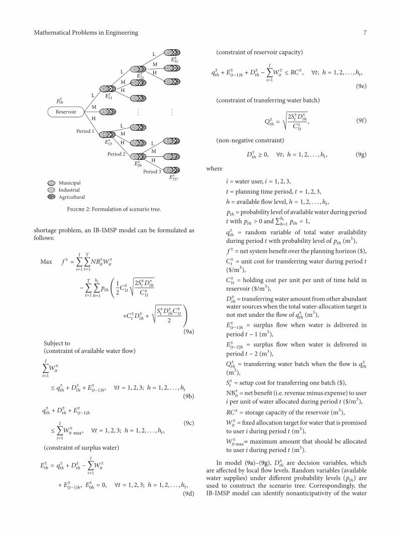