Research Article A spatiotemporal data model for river...

Research Article

A spatiotemporal data model for river basin-scale hydrologic systems

JONATHAN L. GOODALL*{ and DAVID R. MAIDMENT{{Department of Civil and Environmental Engineering, University of South Carolina,

Columbia, SC, USA

{Department of Civil, Architectural, and Environmental Engineering, University of

Texas, Austin, TX, USA

(Received 1 October 2007; in final form 18 January 2008 )

Despite a long history of synergy, current techniques for integrating Geographic

Information System (GIS) software with hydrologic simulation models do not

fully utilize the potential of GIS for modeling hydrologic systems. Part of the

reason for this is a lack of GIS data models appropriate for representing fluid

flow in space and time. Here we address this challenge by proposing a

spatiotemporal data model designed specifically for large-scale river basin

systems. The data model builds from core concepts in geographic information

science and extends these concepts to accommodate mathematical representa-

tions of fluid flow at a regional scale. Space–time is abstracted into three basic

objects relevant to hydrologic systems: a control volume, a flux and a flux

coupler. A control volume is capable of storing mass, energy or momentum

through time, a flux represents the movement of these quantities within space–

time and a flux coupler insures conservation of the quantities within an overall

system. To demonstrate the data model, a simple case study is presented to show

how the data model could be applied to digitally represent a river basin system.

Keywords: Hydrology modeling; GIScience; Spatiotemporal data modeling;

Data integration

1. Introduction

River basin-scale water resource systems require a substantial amount of data to

adequately reconstruct the natural environment in a digital form. The volume of

data is such that scientists and engineers are typically reliant on data products

produced and maintained by outside organizations and individuals to model and

understand how a system functions. This dependence on the data of others

introduces information integration challenges for the water community, challenges

such as data standardization, data fusion and automated access, which are critical to

scientific progress toward managing water resources in a sustainable way.

Geographic Information Systems (GIS) have emerged as a critical tool in

hydrology, in large part because of these information integration challenges. The

technology provides a consistent spatial framework and spatial analysis tools that

allow modelers to gain access to base geospatial datasets such as land use, soils and

terrain, and to derive inputs from these data for their simulation models.

Researchers have proposed a variety of means for coupling a GIS with a hydrology

*Corresponding author. Email: [email protected]

International Journal of Geographical Information Science

Vol. 23, No. 2, February 2009, 233–247

International Journal of Geographical Information ScienceISSN 1365-8816 print/ISSN 1362-3087 online # 2009 Taylor & Francis

http://www.tandf.co.uk/journalsDOI: 10.1080/13658810802032193

Downloaded By: [Ingenta Content Distribution Psy Press Titles] At: 21:23 5 January 2010

model in order to either speed model development time or improve a model’s spatial

representation (Clark 1998; Martin et al. 2005; Sood and Bhagat 2005; Srinivasan

and Arnold 1994; Tim and Jolly 1994). These past approaches can be broadly

grouped into three categories: (1) embedding a GIS within a model (or vice versa);

(2) writing custom software to perform hydrologic modeling routines within a GIS;

(3) automating the exchange of files between the GIS and a model (Martin et al.

2005).

While these past approaches for coupling GIS and hydrology models do present a

way of harnessing the potential of a combined GIS and hydrologic modeling system,

they are often highly pragmatic in how they couple two otherwise independent

software systems. The typical approach has been to build from existing GIS

software technology without consideration of how that software might be altered to

better accommodate hydrologic modeling. While in practice, it is often necessary to

take this approach to quickly and inexpensively build robust systems, the approach

is limiting and restrictive for many hydrologic applications and is therefore not a

suitable long-term solution. We, along with others (Maidment 1996; Sui and

Maggio 1999), argue that the basic disconnection between GIS and hydrology

models is due to the fact that current GIS software does not include a data model

appropriate for representing hydrologic processes, which implicitly limits the types

of hydrology models that can be developed within a GIS context.

For this reason, we propose a new spatiotemporal data model that incorporates

ideas from geographic information science as the basis for creating a river basin-scale

modeling system. The data model provides new building blocks for constructing a

digital representation of a river basin system that begins with concepts such as entities

and fields, but extends these concepts to better align with existing hydrologic modeling

concepts such as control volumes, fluxes, and flows (Reckhow et al. 2004). This data

model provides a generic base from which hydrologic models that make full use of

geospatial analysis algorithms could be constructed.

2. Background

2.1 Representations of hydrologic space–time

There are two basic views of space in geographic information science: space as

comprised of discrete entities and space as a continuous field (Burrough and

McDonnell 1998; Goodchild 1992). Spatial data models most often implement one

of these two basic views of space. For example, a vector data model considers space

as a set of entities, each with a discrete geometry and set of attributes, whereas a

raster data model views space as a continuous field that is sampled and recorded at a

set of fixed locations. Both vector and raster data models are useful for river basin-

scale hydrology applications. Watersheds, rivers and waterbodies are often best

represented as entities using a vector data model, while terrain, precipitation and

land-use are often best represented as a continuous field using a raster data model.

However, although both data models are useful for hydrology applications,

neither is ideally suited to meet the basic needs of representing hydrologic

phenomena. Many researchers have discussed limitations between coupling GIS

with hydrology models (Clark 1998; Srinivasan and Arnold 1994; Sui and Maggio

1999). A fundamental shortcoming is that these data models lack an appropriate

means for representing the transfer of mass, energy and momentum in space and

time. This is in part because existing GIS data models do not include a

234 J. L. Goodall and D. R. Maidment


representation of time (Langran 1992, 1993; Peuquet 2001), but also because they do

not accommodate basic conceptualizations implemented in mathematical models of

hydrologic systems such as control volumes, fluxes and mass balances. These basic

hydrologic conceptualizations used in hydrologic simulation models have been

formulated through the community’s development of simulation models and are,

therefore, better suited for hydrologic analysis when compared to the current data

models available in GIS software.

Despite a near absence of a temporal dimension in most GIS software, various

spatiotemporal data models have been proposed in literature (Erwig and Schneider

2002; Peuquet and Niu 1995; Rasinmaki 2003) and file formats exist for storing

spatiotemporal data. For example, the Network Common Date Form (NetCDF),

which is commonly used in the atmospheric community to store model output from

numerical simulations, implements the concept of storing data in a multidimensional

array that can be both spatial and temporal (Rew and Davis 1990). The Geographic

Markup Language (GML) contains another example of a spatiotemporal data model,

as evident by its specification for dynamic features (Cox et al. 2004). A dynamic

feature is implemented using time stamped instances of a feature with each instance

describing the location and properties of that feature at that moment in time. NetCDF

and GML demonstrate the potential of a spatiotemporal data model for hydrology.

Researchers have proposed geographic data models for hydrology that address

shortcomings in current GIS data models to various degrees, but these data models

are often specific for one hydrologic modeling system. Band et al. (2000), for

example, express a set of hierarchical spatial objects for representing hydrologic

structure and dynamics (i.e. world, basin, hillslope, zone, patch, etc.) and provide a

geographic foundation for the RHESSys watershed model. Likewise, Wang et al.

(2005) describe an object-oriented approach for representing and stimulating a

watershed system built from the TOPMODEL hydrologic model. Our approach is

different in that we propose classes that are specially designed to support

interoperability between multiple modeling systems.

ArcHydro (Maidment 2002) is perhaps the best example of a spatiotemporal data

model of hydrology with the same objective of interoperability, but because

ArcHydro is derived form ESRI ArcObject classes, ArcHydro developers were

required to create spatiotemporal objects through relationships between feature

classes and an object class that stores temporal information. For example, time

series values stored in the TimeSeries object class are related to a station feature

stored in the MonitoringPoint feature class (Figure 1). Here we envision a deeper

integration of space, time and processes through which hydrologic concepts, like

those expressed in ArcHydro, could be more easily implemented. While this

approach would require a programming of GIS software to accommodate natively

spatiotemporal objects, we believe that it is necessary to advance hydrologic

modeling with GIS.

2.2 Hydrologic simulation modeling

Our design of a generic spatiotemporal data model for the hydrologic sciences draws

from both geographic information science as well as a conceptual understanding of

hydrologic simulation modeling. Hydrologic simulation models data from early

conceptualizations like the Rational Method (Chow et al. 1988), a method to

estimate the peak streamflow resulting from a precipitation event, to present day

computer codes such as SWAT, HSPF and HEC-RAS. There are hundreds of

A spatiotemporal data model for hydrologic systems 235


simulation models available for predicting various processes within an overall

hydrologic system (Singh and Woolhiser 2002). Each model is tailored for some

spatial and temporal scale, and to address some scientific or management question.

One way of classifying the existing hydrologic simulation models is by whether

their spatial frame of reference is Eulerian or Lagragian (Maidment 1996). The

Eulerian approach uses a fixed space referencing system where mass and energy

travel through a defined region of space over time. In contract, the Lagragian

approach uses a relative referencing frame where the focus is on following a

particular particle as it travels through a system. Surface water models most often

implement an Eulerian view of space where the model consists of fixed elements

(often called hydrologic response units). The Lagragian view is used to a lesser

extent with examples being particle tracking tools where a ‘slug’ of mass is released

at some location and the model simulates how that slug changes as it travels through

the environment.

Taking a Eulerian approach for analyzing fluid flow, the Reynolds Transport

Theorem can be used to describe how a defined region of space, or a control volume,

stores mass, momentum or energy through time (Chow et al. 1988). If B is either the

property mass, momentum, or energy, then the rate of change of B within a system

(sys) is given by equation (1) where r is the fluid density, b is amount of the fluid

property per unit mass, V is the control volume, ~vv describes the fluid velocity as a

vector, n̂ is a unit vector normal to the control surface and A is the control surface. The

integrations in equation (1) are performed over three-dimensional control volume (cv)

and two dimensional control surface (cs) of the control volume, respectively

dBsys

dt~

d

dt

ðcv

rbdVz

ðcs

rb~vv:n̂dA ð1Þ

Using the Reynolds Transport Theorem, one can derive a water budget by letting

B equal the mass of water m and therefore, because b is the amount of fluid property

per unit mass, it reduces to 1

dmsys

dt~

d

dt

ðcv

rdVz

ðcs

r~vv:n̂dA ð2Þ

Figure 1. Link between space and time in the ArcHydro schema.



This equation provides the basic modeling structure for calculating a water

balance within a GIS. It states that the amount of mass stored within a fixed

boundary system is equal to the rate of change of mass within the control volume

dÐ

cvrdV�

dt� �

, plus the rate at which mass is being transferred across the system’s

boundaries rÐ

cs~vv:n̂dA� �

. One can derive similar expressions for energy and

momentum also using the Reynolds Transport Theorem (Chow et al. 1988).

3. Data model design

3.1 Conceptual design

The Reynolds Transport Theorem consists of two basic conceptualizations of

space–time. The first concept is a control volume: an entity able to store mass,

energy or momentum through time. The second concept is a flux. A flux represents

the transfer of mass, energy or momentum over space and through time. We argue

that space–time can be modeled as a set of control volume and flux objects, where

each control volume may be related to one or more flux objects. The flux objects

that are related to a control volume object describe the exchange of mass, energy or

momentum into or out of that control volume. To ensure conservation within the

overall system, a third concept is needed to specify this coupling between fluxes and

control volumes to ensure that the flux from one control volume is accounted for as

a flux into another control volume (or volumes).

Defining a river basin system as a set of control volumes and fluxes can be carried

out at a variety of spatial and temporal scales. A control volume could be defined

for a continental-scale river basin or an individual grid pixel. Furthermore, it is

possible to represent space as a hierarchy of control volumes where one control

volume is the agglomeration of other, smaller control volumes. For example, a

catchment could be viewed as a control volume where the exchanges of water into

and out of that catchment occur across its land–atmosphere and subsurface

interfaces, and by stream discharge into and out of the catchment. Within a

catchment system, one could define a set of embedded control volumes that might

include such entities as waterbodies or stream channels. The choice as to what to

consider as a unique control volume is left to the modeler and primarily has to do

with the scientific question or management goal at hand. If one wishes to gain

explicit knowledge of the storage of water within a waterbody through time, the

waterbody must be considered as a control volume within the system and not be

lumped into a larger system.

Control volume objects are coupled by the transfer of mass, energy or momentum

through the spatial intersection of their control surfaces. Many existing models

employ a simple spatial structure where cells of a numerical grid share a common

spatial interface. In this case, the flux between control volumes is computed without

an explicit consideration of space. When control volumes are misaligned in space,

however, a spatially-explicit treatment of transfers becomes important to correctly

partition mass, energy or momentum between control volumes. Consider the case

where a watershed model is coupled to an atmospheric model through the exchange

of precipitation and evapotransporation (Figure 2). A grid cell in the atmospheric

model may only partially intersect the receiving watershed control volume, as shown

by the highlighted cell in Figure 2. Using the spatial context for the control volumes,

it is possible to derive the fraction of a quantity transferred between the two control

volumes when they only partially intersect.



A spatially-explicit representation of fluxes associated with control volumes also

requires a careful consideration of dimensions in space, time and measurement

units. A flux is a spatiotemporal quantity, meaning that it has both a spatial

geometry that represents the point, line, or area over which the measurement is

applied, and a temporal geometry that represents the instant or interval of time for

which the measurement is valid (Erwig and Schneider, 2002; Yuan 2004) (Figure 3).

A flux also has measurement dimensions that define the quantity being observed

Figure 2. An example of spatial misalignments between hydrology modeling units: Awatershed with a cell mesh representing atmospheric modeling units.

Figure 3. The combination between a flux’s measurement dimensions and spatialdimensions allows for translation between heterogeneous data sources.



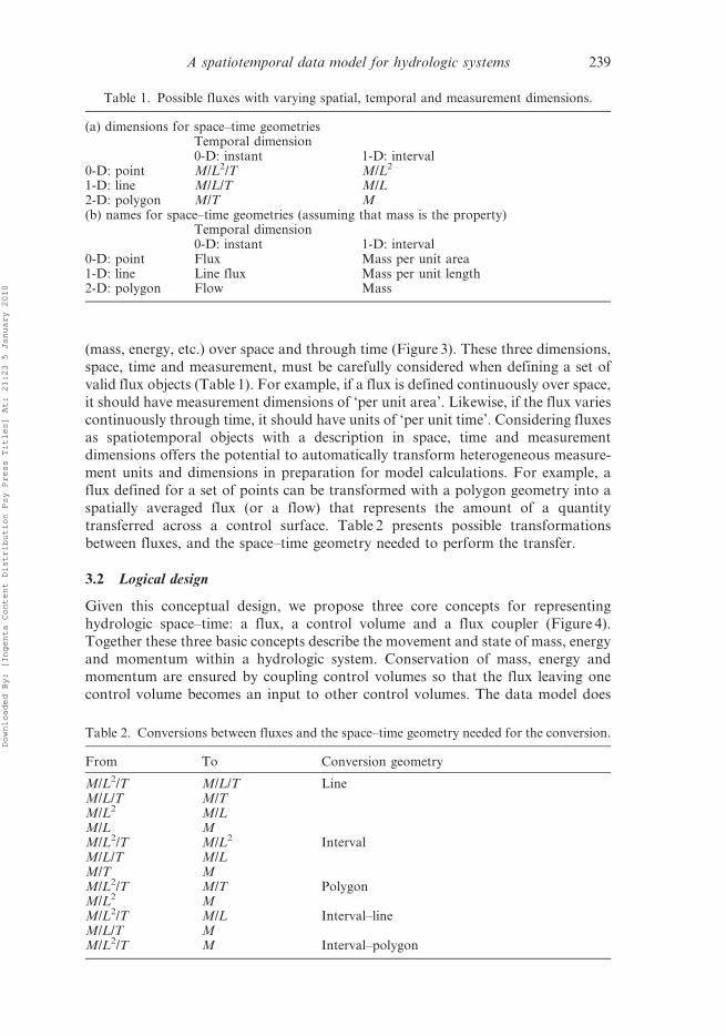
(mass, energy, etc.) over space and through time (Figure 3). These three dimensions,

space, time and measurement, must be carefully considered when defining a set of

valid flux objects (Table 1). For example, if a flux is defined continuously over space,

it should have measurement dimensions of ‘per unit area’. Likewise, if the flux varies

continuously through time, it should have units of ‘per unit time’. Considering fluxes

as spatiotemporal objects with a description in space, time and measurementdimensions offers the potential to automatically transform heterogeneous measure-

ment units and dimensions in preparation for model calculations. For example, a

flux defined for a set of points can be transformed with a polygon geometry into a

spatially averaged flux (or a flow) that represents the amount of a quantity

transferred across a control surface. Table 2 presents possible transformations

between fluxes, and the space–time geometry needed to perform the transfer.

3.2 Logical design

Given this conceptual design, we propose three core concepts for representing

hydrologic space–time: a flux, a control volume and a flux coupler (Figure 4).

Together these three basic concepts describe the movement and state of mass, energy

and momentum within a hydrologic system. Conservation of mass, energy andmomentum are ensured by coupling control volumes so that the flux leaving one

control volume becomes an input to other control volumes. The data model does

Table 1. Possible fluxes with varying spatial, temporal and measurement dimensions.

(a) dimensions for space–time geometriesTemporal dimension0-D: instant 1-D: interval

0-D: point M/L2/T M/L2

1-D: line M/L/T M/L2-D: polygon M/T M(b) names for space–time geometries (assuming that mass is the property)

Temporal dimension0-D: instant 1-D: interval

0-D: point Flux Mass per unit area1-D: line Line flux Mass per unit length2-D: polygon Flow Mass

Table 2. Conversions between fluxes and the space–time geometry needed for the conversion.

From To Conversion geometry

M/L2/T M/L/T LineM/L/T M/TM/L2 M/LM/L MM/L2/T M/L2 IntervalM/L/T M/LM/T MM/L2/T M/T PolygonM/L2 MM/L2/T M/L Interval–lineM/L/T MM/L2/T M Interval–polygon



not assume that control volumes are perfectly aligned in space, so mass balance

calculations could use the spatial intersection between the geometry properties of a

flux coupler object to calculate the contribution of a flux from one control volume

to a second control volume. These types of calculations would be possible because

the system is built from GIS concepts where all objects are spatially referenced

enabling the use of spatial calculations like intersections, interpolations and

aggregations.

A flux object describes the transfer of mass, energy or momentum between control

volumes. Conceptually, a flux can be represented using either a discrete entity or

continuous field view of space. For a discrete entity, the flux has been integrated

over some region of space (either a line or area) and therefore represents a spatially

averaged value. The measurement units of an entity flux must correspond with the

spatial dimensions of its associated geometry. For example, a flux object associated

with a polygon becomes a flow object with units of mass, energy or momentum per

unit time because the flux has been integrated over a two-dimensional surface

(Table 1). A flux could also be associated with a line geometry forming a line flux

with units of mass, energy or momentum per unit length per unit time. As a

continuous field, a flux is associated to a point in space (which can be thought as a

sample of the continuous function) and represents a value with units of per unit time

per unit area.

A control volume object describes a region of space capable of storing mass or

energy. Unlike a flux, a control volume must be represented using an entity view of

space (because a field has no volume), but it can be implemented using either point

geometries, pixels or tessellations. As a geometry, the control volume could

Figure 4. The proposed spatiotemporal data model for representing hydrologic systems atthe river basin scale.



represent a complex, three-dimensional region of space such as a river channel or a

catchment extending from the land surface to the water table. As a pixel or

tessellations, the control volume represents a discretized region of space where each

discretization is able to store quantities through time. In this case, the pixel or

tessellation would represent a three-dimensional volume using a depth attribute

associated with each pixel or tessellation object. An example would be a digital

elevation model (DEM) or a triangulated irregular network (TIN) where each pixel

in the DEM or each triangle in the TIN represents a volume of space extending to

some depth above or below a reference height.

The relationship between control volumes in terms of the fluxes of material

transferred between them is described by a flux coupler object. The flux coupler

object is added to ensure conservation of mass, energy and momentum within an

overall system by ensuring that flux objects describe both the transfer of a property

to and from control volumes. A flux coupler can be thought as a relationship

between control volume objects. While a flux describes the movement of material in

space and time, a flux coupler describes the transfer of material between control

volumes. Thus, a flux coupler consists of a flux object, a source control volume

object and a destination control volume object. It also includes a geometry object

which is the intersection (control surface) through which the transfer occurs.

4. Implementation of the data model: a case study for the Neuse River Basin, North

Carolina

In the following case study the proposed data model is a sample implementation to the

Neuse River Basin in North Carolina (Figure 5). In this case study, the objective is to

represent the river basin system in terms of control volume, flux and flux coupler

objects. This representation allows modelers to more easily derive new properties from

the data, such as the rate of change of water storage within a control volume, because

hydrologic models can be written to operate on the proposed data model. Likewise,

GIS software could be modified to access and visualize the geospatial components of

the data model, or to perform spatial calculations or analysis. GIS and hydrology

models are coupled, therefore, through a common data model that includes a more

robust representation of hydrologic processes in space-time.

For this case study, we populated the data model by starting with the 20 United

States Geological Survey (USGS) streamflow gaging stations within the Neuse River

Basin that have at least 10 consecutive years of daily discharge values. Terrain

processing was then used to generate a single flow path, eight directional flow

direction grid from the 30 m National Elevation Dataset (http://ned.usgs.gov). We

calculated the subwatershed drainage area for each station from the flow direction

grid using the monitoring stations as seed points. Seed points represent the outlets of

subwatersheds. Each subwatershed is therefore the incremental drainage area

between adjacent seed points on the river network. These subwatersheds represent

control volumes within our proposed data model framework, and the stations

represent flux objects.

Consider the subwatershed highlighted in Figure 5. This subwatershed represents

the area draining the land surface upstream of one USGS gage (02089000) and

downstream of three USGS gages (02088000, 02088500 and 02087359). We

considered six fluxes associated with this control volume (three inflows, one

outflow, precipitation and evaporation) and created six flux coupler objects to

describe each exchange between the watershed control volume and other control



volumes within the system (Figure 6). This relationship between control volumes

and fluxes can be captured in an Extensible Markup Language (EML) document

that follows the data model terminology (Figure 7). The root element in the

document is system, and a system element can have one or more control volume, flux

and flux coupler child elements. A control volume is related to one or more flux

elements through the ID attribute of the flux. This structure provides the ability to

store spatiotemporal data about a river basin system and to provide a description of

the transfer of material between control volumes within the system.

In order to estimate change in storage through time for the watershed, historical

daily averaged streamflow measurements were obtained from the USGS National

Water Information System (http://water.usgs.gov/nwis). Precipitation and evapora-

tion fluxes were also obtained from the North American Regional Reanalysis

(NARR) program (http://wwwt.emc.ncep.noaa.gov/mmb/rreanl). The NARR pro-

gram makes use of the current land-surface and atmospheric models to reforecast

past weather conditions, while also assimilating past weather observations from

various sites throughout North America to improve model predictions.

Figure 5. Case study area: the Neuse River Basin in North Carolina. The watersheds werederived from 20 USGS streamflow monitoring stations.



Figure 6. Schematic representation of a control volume in the study domain. The image onthe right represents the streamflows entering and exiting the control volume (q5flow,cv5control volume and fc5flux coupler), while the figure on the right represents thehorizontal fluxes (p5precipitation, e5evaporation, cv5control volume and fc5flux coupler).

Figure 7. An XML representation of the same control volume. A plus sign signifies that theelement has not been expanded to show its contents and an ellipse signifies addition elementscould be inserted to the document.



Streamflow values are recorded by the USGS in units cubic feet per second. This

represents a volume of water per unit time transferred through a channel cross

section. It is possible to estimate a mass flux from these volume flow values by

assuming a density of water, which is a function of the water temperature. Each

streamflow time series represents a flux into one subwatershed and out of a secondwatershed. A flux coupler object accounts for this transfer of mass from the source

watershed to the destination watershed. Precipitation and evaporation are also

fluxes occurring across the boundary of the control volumes and are therefore also

represented as flux coupler objects in the description of the system. NARR provides

these fluxes in dimensions mass per unit area, accumulated over a 3 hour time span.

The values were divided by 3 hours and multiplied by the watershed area to

transform the dimensions into mass per time.

Using these data, change in storage through time (dS/dt) was estimated for theexample subwatershed using the algorithm presented in Figure 8. Thus, the fluxes

for the control volume were converted into consistent dimensions and units and

summed on a daily time step. The results (Figure 9) clearly show the wet (where

dmsys/dt.0) and dry (where dmsys/dt,0) periods for the subwatershed and provide a

sense of the severity of droughts through an estimation of a water deficit. This

process could be repeated for all subwatersheds within the basin to understand how

various regions of the system store water through seasons. It could also be repeated

over a longer temporal domain to identify periods and severity of droughts withinthe basin.

As evident by this simple example of a hydrologic model that operates from the

proposed data model, there are important issues of data transformations that must

be performed to ensure that a mass balance is calculated correctly. For example, if a

flux is not in the dimensions of mass per time, then a calculation is needed to

transform the flux into these dimensions before any water balance calculations. The

proposed data model is intentionally generic and capable of storing multiple

measurement dimensions and units. Data preparation calculations, such as unitconversions, interpolations or integrations, could be systemized and expanded to

Figure 8. Algorithm for calculating change in storage through time from the proposed datamoldel.



Figure 9. Plots of streamflow (a), precipitation and evaporation fluxes (b) and change instorage through time (c).



provide a suite of tools for analyzing river basin systems. The data model would

provide the necessary metadata to enable modeling or analysis software to perform

its own interpreting and transformations of the data before analysis and make it

simpler for scientists to share either own models and analysis tools.

5. Summary

The proposed data model for hydrologic systems combines concepts from

geographic information science and hydrologic science to better enable hydrologic

modeling within GIS. Using the data model, a hydrologic system can be constructed

from basic concepts that define where water is (control volumes), where water

moves (fluxes) and how it is transferred between stores (flux coupler). This data

model provides a view of space–time that is consistent with both hydrology models

and geographic information science concepts. This means that software for

hydrologic modeling and GIS can be written from the data model providing a

new level of integration between hydrology models and GIS.

From the view of geographic information science, the primary benefit of this data

model is that it provides an improved representation for fluid flow within

geographic space. Instead of using generic GIS concepts of features and grids, the

proposed data model introduces concepts of fluxes, control volumes and flux

couplers. From the view of the hydrologic modeler, the primary benefit of the

system is that it provides the ability to harness spatial analysis routines available in

GIS software by enforcing a spatially-explicit representation of hydrologic systems

within the model design itself. One can use this spatial referencing to understand the

coupling between spatially-misaligned control volumes, to operate on values with

different unit dimensions (mass per time, mass per area per time, etc.) and to

integrated or aggregate values across spatial and temporal scales.

Future work will be aimed at creating hydrologic modeling and GIS software

necessary to operate on the proposed data model. This effort should make use of

existing software products to the extent possible, but not be limited by how these

existing software system abstract space and time. Ultimately, the goal is to envision

a new generation of hydrology models and GIS software that are written from

spatiotemporal data models like the one proposed here. This would allow science

and engineering applications to more fully capture real-world hydrologic processes

in space and time with accurate digital representations.

ReferencesBAND, L.E., BRUN, S.E., FERNANDES, R.A., TAGUE, C.L. and TENENBAUM, D.E., 2000,

Modelling watersheds as spatial object hierarchies: structure and dynamics.

Transactions in GIS, 4, pp. 181–196.

BURROUGH, P.A. and MCDONNELL, R., 1998, Principles of Geographical Information Systems

(New York: Oxford University Press).

CHOW, V.T., MAIDMENT, D.R. and MAYS, L.W., 1988, Applied Hydrology. McGraw-Hill

series in water resources and environment engineering (New York: McGraw-Hill).

CLARK, M.J., 1998, Putting water in its place: a perspective on GIS in hydrology and water

management. Hydrological Processes, 12, pp. 823–834.

COX, S., CUTHBERT, A., LAKE, R. and MARTELL, R., 2004, Geography Markup Language

(GML) 3.1.1 OpenGIS Implementation Specification (Wayland, MA: OGC).

ERWIG, M. and SCHNEIDER, M., 2002, Spatio-temporal predicates. IEEE Transactions on

Knowledge and Data Engineering, 14, pp. 881–901.



GOODCHILD, M.F., 1992, Geographical data modeling. Computers and Geosciences, 18, pp.

401–408.

LANGRAN, G., 1992, Time in geographic information systems. Technical issues in geographic

information systems (London/New York: Taylor & Francis).

LANGRAN, G., 1993, Issues of implementing a spatiotemporal system. International Journal of

Geographical Information Systems, 7, pp. 305–314.

MAIDMENT, D.R., 1996, Environmental modeling within GIS. In M.F. Goodchild, L.T.

Stayaert, B.O. Parks, D. Johnston, D.R. Maidment, M. Crane and S. Glendinning

(Eds). GIS and Environmental Modeling: Progress and Research Issues, pp. 147–167

(New York: Oxford University Press).

MAIDMENT, D.R. (Eds), 2002, ArcHydro: GIS for Water Resources (Redlands, CA: ESRI

Press).

MARTIN, P.H., LEBOEUF, E.J., DOBBINS, J.P., DANIEL, E.B. and ABKOWITZ, M.D., 2005,

Interfacing GIS with water resource models: a state-of-the-art review. Journal of the

American Water Resources Association, 41, pp. 1471–1487.

PEUQUET, D.J., 2001, Making space for time: issues in space–time data representation.

Geoinformatica, 5, pp. 11–32.

PEUQUET, D.J. and NIU, D.A., 1995, An event-based spatiotemporal data model (ESTDM)

for temporal analysis of geographical data. International Journal of Geographical

Information Systems, 9, pp. 7–24.

RASINMAKI, J., 2003, Modelling spatio-temporal environmental data. Environmental

Modelling and Software, 18, pp. 877–886.

RECKHOW, K., BAND, L., DUFFY, C., FAMIGLIEI, J., GENEREUX, D., HELLY, J., HOOPER, R.,

KRAJEWSKI, W., MCKNIGHT, D., OGDEN, F., SCANLON, B. and SHABMAN, L., 2004,

Designing hydrologic observatories: a paper prototype of the Neuse watershed.

Technical report (Austin, TX: CUAHSI).

REW, R. and DAVIS, G., 1990, NetCDF – an interface for scientific-data access. IEEE

Computer Graphics and Applications, 10, pp. 76–82.

SINGH, V.P. and WOOLHISER, D.A., 2002, Mathematical modeling of watershed hydrology.

Journal of Hydrologic Engineering, 7, pp. 270–292.

SOOD, C. and BHAGAT, R.M., 2005, Interfacing geographical information systems and

pesticide models. Current Science, 89, pp. 1362–1370.

SRINIVASAN, R. and ARNOLD, J.G., 1994, Integration of a basin-scale water quality model

with GIS. Water Resources Bulletin, 30, pp. 453–462.

SUI, D.Z. and MAGGIO, R.C., 1999, Integrating GIS with hydrological modeling: practices,

problems, and prospects. Computers, Environment and Urban Systems, 23, pp. 33–51.

TIM, U.S. and JOLLY, R., 1994, Evaluating agricultural nonpoint-source pollution using

integrated geographic information systems and hydrologic/water quality model.

Journal of Environmental Quality, 23, pp. 25–35.

WANG, J., HASSETT, J.M. and ENDRENY, T.A., An object oriented approach to the description

and simulation of watershed scale hydrologic processes. Computers and Geosciences,

31, pp. 425–435.

YUAN, M., Representation of space and time. Economic Geography, 2004, 80, pp. 217–218.



Research Article A spatiotemporal data model for river...

Documents

Transcript of Research Article A spatiotemporal data model for river...