Research and investment strategies - Institutional7... · 2017-06-21 · Risk & Reward, #2/2017 3...
46
Theory and practice of portfolio insurance Factor investing: complementing portfolios with customized factor solutions Will President Trump’s fiscal policies lead to a significant rise in inflation? Driverless cars: How innovation paves the road to investment opportunity Risk & Reward Research and investment strategies The document is intended only for Professional Clients and Financial Advisers in Continental Europe (as defined in the important information); for Qualified Investors in Switzerland; for Professional Clients in Dubai, Ireland, the Isle of Man, Jersey and Guernsey, and the UK; for Institutional Investors in Australia; for Professional Investors in Hong Kong; for Qualified Institutional Investors, pension funds and distributing companies in Japan; for Institutional Investors and/or Accredited Investors in Singapore; for certain specific Qualified Institutions/ Sophisticated Investors only in Taiwan and for Institutional Investors in the USA. The document is intended only for accredited investors as defined under National Instrument 45–106 in Canada. It is not intended for and should not be distributed to, or relied upon, by the public or retail investors. #02 2nd issue 2017
Transcript of Research and investment strategies - Institutional7... · 2017-06-21 · Risk & Reward, #2/2017 3...

Theory and practice of portfolio insurance
Factor investing: complementing portfolios with customized factor solutions
Will President Trump’s fiscal policies lead to a significant rise in inflation?
Driverless cars: How innovation paves the road to investment opportunity
Risk & RewardResearch and investment strategies
The document is intended only for Professional Clients and Financial Advisers in Continental Europe (as defined in the important information); for Qualified Investors in Switzerland; for Professional Clients in Dubai, Ireland, the Isle of Man, Jersey and Guernsey, and the UK; for Institutional Investors in Australia; for Professional Investors in Hong Kong; for Qualified Institutional Investors, pension funds and distributing companies in Japan; for Institutional Investors and/or Accredited Investors in Singapore; for certain specific Qualified Institutions / Sophisticated Investors only in Taiwan and for Institutional Investors in the USA. The document is intended only for accredited investors as defined under National Instrument 45–106 in Canada.It is not intended for and should not be distributed to, or relied upon, by the public or retail investors.
#022nd issue 2017

Global editorial committee Chair: Henning Stein and Marlene Konecny. Jutta Becker, Carolyn L. Gibbs, Ann Ginsburg, Dr. Harald Lohre, Kevin Lyman, Jodi L. Phillips, Bruno Schmidt-Voss.
#022nd issue 2017

Risk & Reward, #2/2017 1
My colleagues from the Quantitative Strategies team in Frankfurt have carried out indepth research on this topic, and compared various forms of portfolio insurance. All portfolio insurance strategies share one common goal: setting a limit on the maximum loss of a portfolio. Though in rare circumstances this may not be achieved, a sound portfolio insurance strategy will limit the maximum loss in the vast majority of cases.
Unfortunately – as always in investment – less risk does have a price. Expected returns suffer, and portfolio insurance is no exception. However, at Invesco, we want to make the price of risk mitigation as low as possible.
Traditional static portfolio insurance may be successful in lowering risk, but only at the expense of considerably lower long-term returns. In the old days, when bond yields were high, this may not have been a serious problem. But today’s world is different. When yields are low – or even negative – every percentage point counts. Investors need strategies that think further, and this is what my colleagues have developed.
Using sound quantitative analyses, they have brought forth some very interesting dynamic alternatives. To learn more about the meanings of acronyms such as DPPI and dTIPP – and the advantages that such concepts have over a classic Constant Proportion Portfolio Insurance approach (or CPPI, for short), read our feature – and discover how important it is to invest dynamically when change is the only constant.
The topic of change is also covered by other articles in this edition of Risk & Reward. Our Growth Equity, Fixed Income and Private Capital investment teams have partnered with our Strategy & Innovation team to explore the investment implications of autonomous driving vehicles, which many believe will become one of the megatrends of the coming decades. New technologies have the potential to dramatically change the way we use cars, with far-reaching consequences – even in areas where few expect them. As our numerous examples from different sectors and industries show, the change has already begun.
Regards,
Marty Flanagan President and CEO of Invesco Ltd.
When yields are low and uncertainty is high, investors are faced with a dilemma. Luckily, sophisticated asset managers can offer solutions that help mitigate this dilemma considerably.

Risk & Reward, #2/2017 2
Contents
Feature
4 Theory and practice of portfolio insuranceDr. Martin Kolrep, Dr. Harald Lohre and David Happersberger
To achieve their goals, many investors are allocating towards more risky assets. In many cases, these investors can quickly find themselves in a tight spot if the risk budget is not expanded accordingly. This is where portfolio insurance can come into play. But, which strategy proves to be most effective?
10 “If you drive too fast into every corner, you certainly won’t win the race.”Interview with Dr. Martin Kolrep and Dr. Harald Lohre
Opinions about portfolio insurance are poles apart! We spoke with Dr. Martin Kolrep and Dr. Harald Lohre of the Invesco Quantitative Strategies team, and asked them to say which investors they consider to be best served by portfolio insurance strategies and which concepts to be most appropriate.

Risk & Reward, #2/2017 3
In focus 13 Factor investing: complementing portfolios with customized factor solutionsMichael Abata, Georg Elsaesser, Brad Smith and Jason Stoneberg
When a portfolio has unwanted factor biases, there are several ways to deal with this. One possibility is a factor-based completion portfolio, which we will look at in this article as part of our series on factor investing
17 How macro factors can aid asset allocationJay Raol, Ph.D.
Often, portfolios are built around the correlations between asset classes. But, such an approach is not without its shortcomings. We present an alternative approach that is also based on correlations: but here the focus is on co-movements of asset classes with various macro factors.
24 Will President Trump’s fiscal policies lead to a significant rise in inflation?John Greenwood
Following the election of Donald Trump, equity markets began a significant upward move. At the same time, there has been a sell-off in fixed income markets. We examine the validity of the Trump reflation trade, with respect to US growth prospects, and particularly its possible impact on inflation.
29 Driverless cars: How innovation paves the road to investment opportunityJim Colquitt, Dave Dowsett, Abhishek Gami, Evan Jaysane-Darr, Clay Manley and Rahim Shad
We consider the investment implications of one such game-changing innovation: autonomous driving technology, i.e. driverless cars. The global market for these vehicles is expected to reach the trillion US dollar mark by 2025.
37 The 2017 Cambridge Investment LecturesInvesco’s Cambridge Investment Lectures brought together insights from three leading members of the faculty of the University of Cambridge Judge Business School. Raghavendra Rau, Elroy Dimson and Peter Williamson talked about alternative finance, global investing and opportunities in China.

Risk & Reward, #2/2017 4
In briefTo limit the maximum loss of a portfolio, investment strategies can be enhanced by adding a portfolio insurance component. We have analyzed various portfolio insurance strategies – from the static stop-loss concept to option-based strategies and dynamic portfolio insurance strategies. The findings suggest that an active approach on the basis of dynamic risk forecasts is an effective alternative.
Theory and practice of portfolio insuranceBy Dr. Martin Kolrep, Dr. Harald Lohre and David Happersberger

Risk & Reward, #2/2017 5
end of the year – precluding participation in the significant recovery that followed.
2. Option-based portfolio insuranceAnother static portfolio insurance strategy is the purchase of a European put option.3 Unlike the stop-loss strategy, the put option ensures that the portfolio value will not breach the targeted floor at expiry.
But such a strategy can be expensive, since the option premium is payable on a yearly basis, although the portfolio insurance proves unnecessary in the majority
In order to achieve their performance goals, many investors are allocating towards more risky assets. In many cases, these investors can quickly find themselves in a tight spot if the risk budget is not expanded accordingly. This is where strict risk control via portfolio insurance can come into play. But, which portfolio insurance strategy proves to be most effective in historical simulations?
Investors’ objectives are generally expressed as a combination of risk and return targets. Defining the return target is usually relatively simple – but the definition of risk targets is less straightforward. One conventional approach is to consider “volatility”, that is, the average variation of portfolio return over time. For many investors, however, “maximum drawdown” is a more relevant statistic, as it points to the maximum loss of value. To limit the maximum drawdown, investors typically follow broadly diversified investment strategies that include a tactical asset allocation component designed to avoid losses as often as possible.
However, to effectively limit maximum drawdown, a given investment strategy could implement some form of portfolio insurance. Portfolio insurance strategies aim primarily to improve the downside risk profile of an investment without jeopardizing long-term return potential. In this article, we will present various portfolio insurance strategies and analyze their strengths and weaknesses.
1. Static portfolio insurance using “stop-loss” The stop-loss strategy is an example of a basic portfolio insurance strategy: when the portfolio value falls below a certain threshold (or floor), all risk positions are sold and replaced by risk-free assets (cf. Rubinstein, 1985).
This can be illustrated by looking at a conservative multi-asset portfolio comprising 33.3% equities, 16.7% commodities and 50% fixed income assets.1 Despite this conservative allocation, with 3.9% annualized return and 6.4% annualized volatility in the sample period (July 2003 to November 2016), the maximum drawdown during the 2008 financial crisis was as much as -27.2% (see table 1 at the end of the article).2 To mitigate such losses, we added a stop-loss rule, setting the trigger at a floor of 95% per calendar year (figure 1).
If interest rates are positive, a buffer of more than 5% can be implemented at the beginning of the relevant year; conversely, negative interest rates result in a smaller buffer. The targeted floor is marked by the purple line. It is easy to see that this floor would have been breached from 9 September 2008 onwards – triggering a full reallocation of the portfolio to cash.
This observation reveals a fundamental problem: would a timely exit really have been possible on reaching the 95% threshold in such a volatile period? Moreover, the simple nature of the stop-loss strategy does not envisage a re-entry to the market. In our model, we assume reinvestment at the beginning of the following year. And, although the trigger value is lowered, the marked declines in early 2009 would mean that the portfolio was once again “stopped-out” from 17 February 2009 until the
Figure 1Performance and allocation of the stop-loss strategy
Stop-loss Multi asset portfolio Floor Cash • Exposure (RHS)
Portfolio value Exposure, %
7/03 7/05 7/07 7/09 7/11 7/13 7/15
Investitionsgrad (rechte Skala) Multi-Asset PortfolioCash Stop-LossWertuntergrenze
0
50
100
80
100
120
140
160
180
200
The chart shows the performance of a conservative multi-asset portfolio using a stop-loss strategy (dark blue line) in relation to the floor (purple line) over time. If the portfolio value falls below the floor (here: 95% of the initial annual portfolio value), all risky assets are liquidated. The portfolio is reinvested, if necessary, at the start of the next year. At all events, the floor value is adjusted at the start of each year to accommodate investment. For comparison, we have included the performance of the underlying conservative multi-asset strategy (light blue line) and a money market investment (green line).Sources: Bloomberg, Invesco. Period: 23 July 2003 to 22 November 2016; 23 July 2003 = 100.
Figure 2Performance and allocation of the synthetic put strategy
Synthetic put Multi asset portfolio Floor Cash • Exposure (RHS)
Portfolio value Exposure, %
7/03 7/05 7/07 7/09 7/11 7/13 7/15
Investitionsgrad (rechte Skala) Multi-Asset-PortfolioCash Synthetischer PutWertuntergrenze
0
50
100
80
100
120
140
160
180
200
The chart shows the performance of a conservative multi-asset portfolio using a synthetic put strategy (dark blue line) in relation to the floor (purple line) over time. Participation in the risky asset’s performance is calculated using a classic Black-Scholes formula measuring the sensitivity of a synthetic put with a strike price matching the floor value (here: 95% of the initial annual portfolio value). For comparison, we have included the performance of the underlying conservative multi-asset strategy (light blue line) and a money market investment (green line).Sources: Bloomberg, Invesco. Period: 23 July 2003 to 22 November 2016; 23 July 2003 = 100.

Risk & Reward, #2/2017 6
of cases. Moreover, it is often not easy to find option contracts that fit the needs of the portfolio – particularly when it comes to complex investment vehicles like the proposed multi-asset portfolio. Yet, both of these problems can be addressed by synthetically replicating the necessary European put option, which ultimately consists in dynamically adjusting the investment exposure of the multi-asset portfolio.4
Figure 2 charts the evolution of the synthetic put strategy over time. We note that the rate of investment (exposure) varies significantly, depending on the difference between the portfolio value and the strike price, as well as expected volatility.5 Unlike the stop-loss strategy, exposure would have been reduced early enough in 2008 to avoid a massive drawdown. Yet, it was still at 44% when the floor was first breached in 2008; by the end of the year, the portfolio value would have been 4% below the floor value. This demonstrates one weakness of a synthetic put strategy, which also has the disadvantage of frequent portfolio reallocation. Nonetheless, the synthetic put strategy would have made far better use of the subsequent market recovery than the stop-loss strategy. Ultimately, performance would have matched that of the underlying multi-asset portfolio – with substantially less volatility and a lower maximum drawdown.
3. CPPI and related dynamic portfolio insurance strategiesGiven the shortcomings of option-based portfolio insurance, an alternative can be found in a dynamic variant of the classic CPPI (constant proportion portfolio insurance6) strategy. First, we will examine the CPPI concept itself, before looking deeper into dynamic portfolio insurance.
3.1 CPPIAt the heart of the classic CPPI strategy is the so-called cushion Ct, i.e. the difference between the invested capital (or wealth), Wt and the net present value of the floor NPV (FT):
(1) C W NPV Ft t T= − ( )In order to avoid a breach of the floor, the risky investment Et = et × Wt (with investment exposure et) should be set such that:
(2) C W W
C e W risky asset
EC
r
t t t
t t t
tt
≥ × ( )≥ × × ( )
≤
MaxLoss
MaxLoss
MaxLoss iisky assetm Ct( )
= ×
In this context, the multiplier
mrisky asset
:=( )1
MaxLoss
allows for a neat interpretation: it indicates how often a given cushion can be invested in the risky asset without breaching the floor assuming that the maximum loss assumption of the risky asset is not violated.
The classic CPPI strategy is based on a static multiplier – often reflecting a constant worst-case
scenario. Figure 3 illustrates the performance and exposure of a CPPI strategy, which assumes a constant maximum overnight loss of 3%, which is equivalent to the historically simulated expected shortfall (ES) of the multi-asset portfolio. Although this very conservative position would have prevented catastrophic drawdowns during the financial market crisis, it would also have left significant return potential unused over the long term. This is reflected in the average investment exposure of just 70.2% – pushing annualized returns down a full 75 bp to a mere 3.14% p.a. (see table 1 at the end of the article).
3.2 DPPIThis is where dynamic proportion portfolio insurance (DPPI) proves its effectiveness. Instead of using a static multiplier, the risk budget adapts dynamically to changes in expected shortfall (ES). Exposure is set such that:
(3) EC
risky assetm Ct
t
tt t≤
( )= ×
MaxLoss
with the multiplier
mES risky asset
tt
:%
=( )
199
In this way, the exposure of the portfolio reacts to changes in the risk forecast – ensuring that it does not remain artificially low as a result of a constant conservative risk assumption. For this to work in practice, the risk model must be capable of quickly homing in on volatility spikes, and just as quickly readjusting to a normalization of market volatility. To this end, a Copula-GARCH model is extremely useful for forecasting ES (see box: Risk forecasting for dynamic portfolio insurance strategies).
We start by setting the exposure in accordance with equation (3). Figure 4 shows that, although the DPPI
Figure 3Performance and allocation of the CPPI strategy
CPPI strategy Multi asset portfolio Floor Cash • Exposure (RHS)
Portfolio value Exposure, %
0
50
100
7/03 7/05 7/07 7/09 7/11 7/13 7/15
Investitionsgrad (rechte Skala) Multi-Asset-PortfolioCash CPPIWertuntergrenze
80
100
120
140
160
180
200
The chart shows the performance of a conservative multi-asset portfolio using a CPPI strategy (dark blue line) in relation to the floor (purple line) over time. Exposure is calculated using the cushion (difference between the portfolio value and the floor; here: 95% of the initial annual portfolio value) and the multiplier that is based on daily risk forecasts of the historically simulated ES of the multi-asset portfolio (3%). For comparison, we have included the performance of the underlying conservative multi-asset strategy (light blue line) and a money market investment (green line). Sources: Bloomberg, Invesco. Period: 23 July 2003 to 22 November 2016; 23 July 2003 = 100.

Risk & Reward, #2/2017 7
strategy actively adjusts exposure, it fluctuates to a lesser degree than with the synthetic put. With the onset of the financial market crisis, exposure dropped to zero, so that the portfolio value at the end of 2008 was equal to the floor. Then, even with the V formation (steep decline followed by a rapid recovery) in early 2009, which is a major pitfall for
portfolio insurance, the DPPI portfolio did not end up like the stop-loss in a “cash lock” within the money market. It participated in at least part of the subsequent recovery.
On the whole, the DPPI strategy actually delivered a marginal excess return compared with the pure
Modern risk modelling is guided by empirical patterns, which cannot be adequately captured using a conventional approach with an assumption of normal distributions. In particular, extreme events occur substantially more often than postulated by a normal distribution. Volatility and correlations are not constant, and volatility-clustering is not uncommon.
An effective method of understanding empirical risk is the Copula-GARCH model, as proposed by Patton (2006) or Jondeau and Rockinger (2006): the GARCH component measures the risk dynamics, while the copula estimation permits adequate modelling of the dependence structure.
Another matter to consider, in addition to the structure of the model itself, is the question of an appropriate risk measure. Whereas many risk management approaches rely on value-at-risk (VaR), portfolio insurance strategies naturally lend themselves to using expected shortfall (ES) to measure risk. In the case of VaR, it indicates the maximum possible loss at a given confidence level (usually 95% or 99%). However, VaR is silent with respect to the losses beyond the VaR threshold. Conversely, the ES measures the expected loss in the event of a VaR violation.
Validity of VaR and ES forecastsThe validity of Copula-GARCH risk forecasts can be demonstrated using various statistical tests. In order to have a sound basis for the estimated ES, the corresponding VaR quantile must be correctly specified. In a set of 260 forecasts of 1-day VaR (99% confidence) per year, there should theoretically be 2.6 violations. The upper panel of the chart shows a very simple VaR forecast as given by the empirical VaR over a sliding 1,000-day window. As expected, the majority of realized returns were higher than the forecasted VaR. In the sample period from July 2003 to November 2016, there were only 32 violations (pink dots) – which is nearly the same as the 35 expected (= 1% of 3.479).
An analysis of the VaR violations throughout time is sufficient to call into doubt the utility of the historically simulated VaR – given that nearly all of them occurred during the 2008 financial market crisis due to a latent underestimation of risk. Subsequently, the historically simulated VaR forecast was overly conservative, and there were no more violations for five years. Thus, a portfolio insurance strategy on this basis would have held investment exposure much too low over time.
This conclusion is confirmed by rigorous statistical testing. Using the unconditional coverage test (Kupiec, 1995), the historically simulated VaR does indeed deliver a conclusive number of violations over the entire period. But, based on the test for
correct coverage and independence (Christoffersen, 1998) and the duration test (Christoffersen and Pelletier, 2004), it is clear that the violations are not independently occurring, but rather appear in clusters.
The lower panel of the chart shows the VaR forecast on the basis of the Copula-GARCH model, which is much more sensitive and quick to react to the prevailing risk environment. The 35 violations over the entire period are precisely in line with the theoretical expectation; moreover, their occurrence is markedly less clustered – as confirmed by the statistical tests. And: the ES estimator corresponding to the Copula-GARCH VaR quantile also passes the so-called “zero mean” test proposed by McNeil and Frey (2000), i.e. the excess losses are independently distributed around a mean of zero.
Box Risk forecasting for dynamic portfolio insurance strategies
VaR-forecasts and realized returns of the multi-asset portfolio Realized return Historically simulated VaR • VaR violation%
-6
-4
-2
0
2
4
7/03 7/05 7/07 7/09 7/11 7/13 7/15
Realisierte Rendite Historischer VaR Rendite<VaR
Realized return Copula-GARCH-VaR • VaR violation%
-6
-4
-2
0
2
4
7/03 7/05 7/07 7/09 7/11 7/13 7/15
Realisierte Rendite GARCH-Copula-VaR Rendite<VaR
The chart shows the daily VaR forecasts (blue line) and realized returns of the multi-asset portfolio (grey dots) over time. VaR violations are marked in pink. At a confidence level of 99%, a total of 35 violations are expected over the model period. Both historically simulated VaR (above) and Copula-GARCH VaR (below) exhibit the expected number of violations on average – but only under the Copula-GARCH VaR forecast are these violations independent and non-clustered. Sources: Bloomberg, Invesco. Period: 23 July 2003 to 22 November 2016.

Risk & Reward, #2/2017 8
multi-asset strategy (3.98% return; 4.69% volatility – see table 1 at the end of the article). Compared to the stop-loss and synthetic put, the maximum drawdown is significantly lower (by approx. 4 percentage points). Thus, the portfolio insurance can be achieved without the purchase or replication of an option, and can also be easily and flexibly adapted to accommodate changing investment demands.
4. Dynamic portfolio insurance with a “ratchet floor”: the TIPP
A more conservative alternative to the CPPI strategy is the so-called TIPP (time invariant portfolio protection) strategy. In essence, it complements the CPPI strategy by locking in a portion of gains achieved with the portfolio. The floor is “ratcheted-up” as soon as a new high is reached in portfolio value. Figure 5 shows the development of a dynamic TIPP strategy (dTIPP), based on the identical ES risk forecast as the DPPI strategy. Exposure over the entire period is roughly 10 percentage points lower than that of the DPPI strategy – a consequence of the floor always being closer to the portfolio value so that no additional cushion can be built up. This implies a clear reduction of returns vs. DPPI – but one that is less dramatic in risk-adjusted terms.
ConclusionOur examination has shown that dynamic portfolio insurance could be useful in improving the risk-return profile of an investment (table 1). The most attractive alternative we have found was the DPPI strategy – an improvement on the classic CPPI strategy. Because DPPI works with a dynamic measure of risk, it adapts much more readily to the market environment than the CPPI approach with its constant multiplier. Moreover, in terms of the Sharpe ratio, maximum drawdown and investment exposure, the DPPI strategy outperformed the stop-loss, the synthetic put and the dTIPP strategy.
Figure 4Performance and allocation of the DPPI strategy
DPPI strategy Multi asset portfolio Floor Cash • Exposure (RHS)
Portfolio value Exposure, %
7/03 7/05 7/07 7/09 7/11 7/13 7/15
Investitionsgrad (rechte Skala) Multi-Asset-PortfolioCash DPPIWertuntergrenze
0
50
100
80
100
120
140
160
180
200
The chart shows the performance of a conservative multi-asset portfolio using a DPPI strategy in relation to the floor over time. Exposure is calculated using the cushion (difference between the portfolio value and the floor; here: 95% of the initial annual portfolio value) and the multiplier (based on daily risk forecasting; here: Copula-GARCH 99%-ES). For comparison, we have included the performance of the underlying conservative multi-asset strategy and a money market investment. Sources: Bloomberg, Invesco. Period: 23 July 2003 to 22 November 2016; 23 July 2003 = 100.
Figure 5Performance and allocation of the dTIPP strategy
dTIPP strategy Multi asset portfolio Floor Cash • Exposure (RHS)
Portfolio value Exposure, %
0
50
100
7/03 7/05 7/07 7/09 7/11 7/13 7/15
Investitionsgrad (rechte Skala) Multi-Asset-PortfolioCash dTIPPWertuntergrenze
80
100
120
140
160
180
200
The chart shows the performance of a conservative multi-asset portfolio using a dTIPP strategy in relation to the floor over time. Exposure is calculated using the cushion (difference between the portfolio value and the floor; here: 95% of the initial annual portfolio value each year) and the multiplier (based on daily risk forecasting; here: Copula-GARCH 99%-ES). The key characteristic of the dTIPP strategy lies in the “ratcheting-up” of the floor (95%) once a new high is achieved. For comparison, we have included the performance of the underlying conservative multi-asset strategy and a money market investment. Sources: Bloomberg, Invesco. Period: 23 July 2003 to 22 November 2016; 23 July 2003 = 100.
Table 1Figures for the conservative multi-asset portfolio with and without portfolio insurance
Multi asset portfolio Money market investment Stop loss Synthetic put DPPI dTIPP
Return p.a. (%) 3.89 1.23 3.65 3.89 3.98 3.45Volatility p.a. (%) 6.40 0.11 5.04 4.71 4.69 4.05Sharpe ratio 0.42 0.00 0.48 0.56 0.59 0.55Maximum drawdown (%) -27.16 0.00 -14.49 -14.28 -10.43 -8.82Exposure (%) 100.00 0.00 91.09 89.58 90.37 80.38
The table shows the performance figures for the various portfolio insurance strategies in combination with a multi asset portfolio: stop-loss, synthetic put, constant proportion portfolio insurance (CPPI), dynamic proportion portfolio insurance (DPPI) and dynamic time invariant portfolio protection (dTIPP). In each calendar year, a floor of 95% of the initial portfolio value is targeted. For comparison, we have included the performance figures for the underlying conservative multi-asset strategy and a money market investment. Sources: Bloomberg, Invesco. Period: 23 July 2003 to 22 November 2016.

Risk & Reward, #2/2017 9
Bibliography• Black, F. and Jones, R. (1987). Simplifying
portfolio insurance. Journal of Portfolio Management 14, 48–51.
• Black, F. and Jones, R. (1988). Simplifying portfolio insurance for corporate pension plans. Journal of Portfolio Management 14, 33–37.
• Christoffersen, P. (1998). Evaluating interval forecasts. International Economic Review 39, 841–862.
• Christoffersen, P. and Pelletier, D. (2004). Backtesting value-at-risk: A duration-based approach. Journal of Financial Econometrics 2(1), 84-108.
• Dichtl, H., and Drobetz, W. (2011). Portfolio insurance and prospect theory investors: Popularity and optimal design of capital protected financial products. Journal of Banking and Finance 35, 1683-1697.
• Estep, T. and Kritzman, M. (1988). TIPP: Insurance without complexity. Journal of Portfolio Management 14, 38–42.
• Jondeau, E. and Rockinger, M. (2006). The Copula-GARCH model of conditional dependencies: An international stock market application. Journal of International Money and Finance 25, 827-853.
• Kupiec, P. H. (1995). Techniques for verifying the accuracy of risk measurement models. The Journal of Derivatives 3(2), 73-84.
• McNeil, A. J., and Frey, R. (2000). Estimation of tail-related risk measures for heteroscedastic financial time series: An extreme value approach. Journal of Empirical Finance 7(3), 271-300.
• Patton, A. J. (2006). Modelling asymmetric exchange rate dependence. International Economic Review 47(2), 527-556.
• Perold, A. F. (1986). Constant proportion portfolio insurance. Working paper, Harvard Business School.
• Perold, A. F. and Sharpe, W. F. (1988). Dynamic strategies for asset allocation. Financial Analysts Journal 44, 16–27.
• Rubinstein, M. (1985). Alternative paths to portfolio insurance. Financial Analysts Journal 41, 42-52.
• Rubinstein, M. and Leland, H. E. (1981). Replicating options with positions in stock and cash. Financial Analysts Journal 37, 63–72.
About the authors
Dr. Martin KolrepSenior Portfolio Manager, Invesco Quantitative StrategiesDr. Martin Kolrep is involved in the development of client solutions and the management of multi asset strategies.
Dr. Harald LohreSenior Research Analyst, Invesco Quantitative StrategiesDr. Harald Lohre develops quantitative models to forecast risk and return used in the management of multi-asset strategies.
David HappersbergerPhD Candidate Lancaster University, Invesco Quantitative StrategiesAs part of a joint research initiative between Lancaster University and Invesco Quantitative Strategies, David Happersberger is pursuing post-graduate work on practice-oriented issues of financial market econometrics. At the same time, he is actively supporting the transfer of research results into the multi-asset investment process.
Notes1 Throughout the article and in all figures and tables, the multi-asset data set consists of the
following series (portfolio weights are given in parentheses): EuroStoxx 50 Future (5.8%), FTSE 100 Index Future (5.8%), S&P500 Future (15%), Nikkei 225 Future (6.7%), Euro-Bund Future (16.7%), US 10YR Note Future (16.7%), JPN 10Y Bond Future (16.7%), S&P GSCI Crude Oil (3.5%), S&P GSCI Gold (5.8%), Bloomberg Agriculture Subindex (3.8%), Bloomberg Copper Subindex (3.5%). For money market investments we use the 3-month US Treasury bill. All asset returns are in local currency. Portfolio returns and values are computed from the perspective of an U.S. investor who is hedging any currency exposure. Furthermore, all simulations in this article are provided for illustrative purposes only and are subject to limitations. Unlike actual portfolio outcomes, the model outcomes do not reflect actual trading, liquidity constraints, fees, expenses, taxes and other factors that could impact future returns.
2 Table 1 at the end of the article shows the performance figures for all of the strategies presented.
3 A European option can only be exercised at expiry (unlike an American option, which can be exercised at any time during its term).
4 Delta, i.e. the sensitivity of the synthetic put option to changes in the underlying, is determined using the classic Black-Scholes model. The strike price is set to reflect the desired floor value (Rubinstein and Leland, 1981; Dichtl and Drobetz, 2011).
5 A volatility forecast is necessary to determine delta and we build on a Copula-GARCH model (see box: Risk forecasting for dynamic portfolio insurance).
6 For more on CPPI strategies, cf. Perold (1986), Black and Jones (1987, 1988), Perold and Sharpe (1988).

Risk & Reward, #2/2017 10
“ If you drive too fast into every corner, you certainly won’t win the race.”
Interview with Dr. Martin Kolrep and Dr. Harald Lohre
For some, it’s no more than a cost factor with no long-term benefit. For others, it’s the key to unifying short-term and long-term goals in portfolio management. In short: opinions about portfolio insurance are poles apart! We spoke with Dr. Martin Kolrep and Dr. Harald Lohre of the Invesco Quantitative Strategies team, and asked them to say which investors they consider to be best served by portfolio insurance strategies and which concepts to be most appropriate.
Risk & RewardGenerally speaking, portfolio insurance costs investors some of their long-term returns. So, why should they still consider it?
Dr. Harald LohreThat depends largely on the situation of the investor. Long-term investors with deep pockets might be able to get by without portfolio insurance.
Dr. Martin KolrepUnfortunately, reality is not often that simple. For various reasons, many investors today can no longer maintain a long-term horizon, but have to deal with short-term realities. These can include legal requirements like the new IFRS 9 accounting standard1 – which will be of growing importance for investors worldwide from now on. When financial market losses are carried directly to the balance sheet, many investors will have to pay more attention to the volatility and loss risks in their portfolios, and find ways to limit both. In such circumstances, costs and a minor sacrifice of return potential could be secondary.
Dr. Martin Kolrep Senior Portfolio Manager Invesco Quantitative Strategies
Dr. Harald LohreSenior Research Analyst Invesco Quantitative Strategies

Risk & Reward, #2/2017 11
Risk & RewardYet, for several years now, with prices moving steadily higher, you get the impression that portfolio insurance has become obsolete. Is it really necessary in these markets?
Dr. Harald LohreDoing without portfolio insurance would be like terminating fire insurance on your home because you haven’t had a fire in ten years. It may not be a wise move.
Dr. Martin Kolrep There is no doubt that many investors tend to view the recent past as ‘the new normal’. Anything that happened further in the past is ignored. The sensible thing would be to look back at earlier periods of disruption with scenario analyses to simulate performance of the current portfolio in those situations. This often provides insights that underscore the need to consider portfolio insurance.
Risk & RewardBut, as a neutral observer, you sometimes get the impression that mechanistic portfolio insurance strategies serve to reduce risks just when it’s least necessary. What would you say to that?
Dr. Martin Kolrep The first step is always to set up a strategic asset allocation in accordance with the investor’s medium-term risk profile. This should generally include a broad diversification of the portfolio. This on its own can minimize the probability of needing to limit exposure due to risk – in fact substantially so.
Dr. Harald LohreStep two is to carry out a tactical assessment of the markets. If a certain asset class is expected to hurt portfolio performance, tactical allocation can be used as an early defence. In other words, investors should ideally be able to navigate through turbulent markets on the basis of tactical positioning alone. But market forecasts are rather uncertain, making it impossible to correctly anticipate every eventuality. This is precisely where the third step of risk management and portfolio insurance can step into action: reducing investment exposure as the ultima ratio, striving to protect portfolio value.
Risk & Reward Can a risk-return profile on par with an equity investment be achieved when implementing a portfolio insurance strategy?
Dr. Martin KolrepOf course. A portfolio insurance strategy allows investors to participate in an asset class while specifying the desired level of risk. And, when you see long-term average volatility of 15% to 20% in the equity market, do you really have to sit by passively and accept that? What about an investor who is constrained to a maximum volatility of only 8%? Or a 15% maximum drawdown? Do they deserve to be locked out from equities? Today, we have possibilities of replicating the return profile of the equity market while keeping volatility at a constant, say 8%. But, it is also possible to simply cut out volatility spikes.
Dr. Harald LohreNaturally, you can’t expect returns to exactly match what you would see with a pure equity investment – but that is also missing the point. The idea that high volatility is the price for equity-like returns is now archaic. That can be achieved – with a smaller exposure – at lower rates of risk. And, if equities are one of the few remaining attractive asset classes, this could be in the interest of investors – especially those with a limited risk budget.
Risk & RewardSo for which investors could portfolio insurance strategies be particularly relevant?
Dr. Harald LohreIn principle, these strategies can be a good idea for any investors who value preventing short-term losses over maximizing long-term returns. Not every investor can follow the ‘buy-and-hold’ principle. Some investments may end up proving much more volatile than expected in the next crisis. If investors wait until then to think about limiting risk, they could end up having to sell at the worst-possible moment – namely, when they can no longer tolerate high risks.
Dr. Martin KolrepIt happens again and again. It’s like a racing car driver keeping the accelerator pedal fixed to the floor, even in the corners. If you drive too fast into every corner, you certainly won’t win the race – even if you are sometimes the fastest on the track. It makes much more sense to target a speed that is appropriate to the course and respects the other drivers. That way, you could reach your objectives without too much wasted effort – admittedly a position that is more difficult to communicate in an era of very low interest rates.
Risk & RewardIn your article, you argue that a dynamic approach to portfolio insurance based on econometric risk models is the most effective alternative. Why not just buy a put option to avoid going ‘too fast into the corners’?
Dr. Harald LohreUsing an option-based strategy does give a margin of certainty that the value of the portfolio won’t fall below a floor value. But, there are costs to consider, in the form of option premiums – even in years when the option is not exercised. This means that costs can be higher than necessary. And, there is not always a suitable put available to hedge the risks of a diversified multi-asset portfolio. In such cases, a tailored hedge must in effect be put in place for each individual position, meaning even more costs.
Dr. Martin KolrepBut by pursuing a dynamic strategy instead, investors can focus on certain extreme overnight risks – gap risks. In some exceptional cases, the market could open at prices lower than can be upheld by the floor. This risk can be minimized substantially through worldwide investments and broad diversification of the portfolio, which make it unlikely that an event like this would impact all positions in the same way.

Risk & Reward, #2/2017 12
Risk & RewardThen I guess the liquidity of the investments must be very important. What happens if a portfolio ends up in a liquidity bind?
Dr. Martin Kolrep That must best be avoided. We aim to prevent this today by investing only in instruments that are highly liquid – and which have remained so in periods such as the financial market crisis. It’s highly unlikely that a time will come when nobody is buying in the major equity markets. What's far likelier is that prices continue to fall until buyers are found. The corporate bond market is a possible exception. In times of crisis, corporate bond spreads could widen to the point at which no buyers can be found, no matter the price – which is why our own multi-asset strategy does not invest in corporate bonds.
Risk & RewardBack to the topic of portfolio insurance – what is it about a dynamic portfolio insurance strategy that makes it so exceptional?
Dr. Martin Kolrep Simple: the dynamic approach can give investors more exposure in normal markets. Ultimately, you have to anticipate when volatility will be low and when it will be high. In phases of low volatility, a high exposure should be considered, in order to profit from rising prices. But, when volatility picks up, investors should consider reducing their exposure as rapidly as possible.
Dr. Harald LohreThis is also why it’s so important to develop a cutting edge risk model, which can accurately forecast changes in volatility in order to adapt the portfolio allocation. To this end, a Copula-GARCH model delivers strong signals – as the market data input is a good barometer of market anxieties.
Dr. Martin KolrepThink of a seismograph: you can use the data collected to help predict volcanic eruptions. You can’t tell whether a volcano is about to erupt by walking up to the rim of the caldera. It might be exciting and interesting – but it’s not going to give you insight into what's going to happen next.
Dr. Harald LohreIt works the same way in capital markets. People often have difficulty identifying how a certain event will change the risk environment. This is why we trust in solid empirical forecasting models, which have proven their worth – especially in conjunction with dynamic portfolio insurance strategies.
Dr. Kolrep, Dr. Lohre, thank you for your time.
Note1 IFRS 9 is an International Financial Reporting Standard (IFRS) promulgated by the
International Accounting Standards Board (IASB). It addresses the accounting for financial instruments. It contains three main topics: classification and measurement of financial instruments, impairment of financial assets and hedge accounting. It will replace the earlier IFRS for financial instruments, IAS 39, when it becomes effective in 2018 (Wikipedia).

Risk & Reward, #2/2017 13
In briefWe examine two approaches to complementing existing portfolios with customized factor solutions, both of which are aimed at improving their risk/return characteristics. After determining the factor tilts in existing portfolios, the first approach uses the broad range of available factor-based ETFs to achieve the desired risk-adjusted return. The second approach is actively managed: we develop a highly customized factor completion portfolio that reflects a client’s individual risk/return targets as fully as possible. We find that both approaches lead to meaningful improvements, as confirmed by a wide range of statistics such as expected alpha, tracking error and information ratio.
Factor investing: complementing portfolios with customized factor solutionsBy Michael Abata, Georg Elsaesser, Brad Smith and Jason Stoneberg
When a portfolio has unwanted factor biases, there are several ways to deal with this. One possibility is a factor-based completion portfolio, which we will look at in this article as part of our series on factor investing.
It is well established that a meaningful proportion of a portfolio’s performance is explained by exposure to factors that drive risk and return. Further research has shown that certain factors have historically been more apt at delivering risk-adjusted excess returns.1 This has long been understood by quantitative asset managers, who build multi-factor portfolios in order to harvest such premiums. While these portfolios generally provide well-balanced factor exposure in isolation, they often fail to account for an investor’s existing investments.
As with any portfolio, these existing investments also have factor exposures. For example, we looked at the factor tilts of more than six hundred actively managed US large cap funds. On average, relative to the S&P 500 Index, these funds were underweight on low volatility and dividend yield, while being neutral on momentum, quality and value and overweight on small size. Needless to say, an individual portfolio or subset of portfolios would likely see more substantial factor tilts than the average.
To construct a portfolio with balanced factor exposure, it is therefore important to understand the factor tilts implicit in an initial portfolio. Once these tilts

Risk & Reward, #2/2017 14
and tracking error was reduced for 91%. The averages of all 642 funds also improved: annualized total returns in USD increased by 50 bps, volatility (i.e. standard deviation of returns) decreased by 71 bps and tracking error decreased by 132 bps.
Actively managed completion portfoliosThe second approach uses actively managed completion portfolios. Our aim was to increase portfolio risk-adjusted return and diversify specific (idiosyncratic) risk, while mitigating exposure to known common risk factors and increasing exposure to desired alpha signals. We show results for two portfolios, a US portfolio benchmarked to the S&P 500 and a non-US portfolio benchmarked to the MSCI EAFE index. In each case, the completion sleeve is allocated 35% of total portfolio capital. Simulations were run for the ten-year period from January 2006 to December 2016.3
The objective was to reduce risk to a desired range relative to a benchmark: in both the US and the non-US case, we were looking to target tracking error against the respective benchmark at between 275 and 325 bps.
have been measured, a completion portfolio can be constructed. Taken together, the two portfolios should exhibit the desired factor exposures (figure 1).
Completion portfolios can be implemented in various ways, ranging from blends of passive factor ETFs to custom-built actively managed portfolios. Depending on scale, customization and cost, investors may choose to have their completion portfolios actively managed or to implement their own completion portfolios using ETFs.
Completion portfolios using factor ETFsETFs are liquid, transparent and tradable vehicles that can provide targeted exposure to individual factors, including: value, momentum, low volatility, quality, small size and dividend yield. They can provide a vast array of options to build custom factor blends, including those which are needed to build custom completion portfolios in a low-cost, efficient manner. For instance, if an investor needed 70% momentum and 30% quality to balance an existing portfolio’s factor exposure, this could easily be achieved by blending together two ETFs.
To study the efficacy of this approach, we built completion portfolios for 642 actively managed US large cap funds, which have at least ten years of history and are categorized as US Large Cap Growth, Large Cap Blend or Large Cap Value by Morningstar.2 Our long-only completion portfolios were formed from the S&P 500 low volatility, momentum, enhanced value and quality factor indices. In all cases, an allocation of 30% was given to the completion portfolio with 70% remaining in the active mutual fund.
Each fund’s completion portfolio was created by solving for the blend of factor indices that had the lowest correlation of excess returns to the fund, based on five years of monthly returns from 2007 to 2011. The completion portfolios were permitted to include up to four of the factor indices, depending on the appropriate blend. Performance of the initial fund, plus the completion portfolio, was measured from 2012 to 2016. According to our results, adding the completion portfolio led to an improvement of multiple performance and risk statistics.
A wide range of measures have improvedFigure 2 shows that, by adding a completion portfolio, the portfolio statistics improved for the majority of the funds. For 80% of the funds, annualized returns increased; volatility decreased for 81% of the funds
Figure 2An ETF-based completion portfolio has led to better metrics for the majority of funds
% with improvement
81%
93%98% 96%
76%80%
91%98%
60%
45%
81%
Ann
ualiz
ed r
etur
n
Alp
ha t
o S
&P
500
Ris
k ad
just
ed r
etur
n
Sort
ino
ratio
Wor
st 1
2 m
onth
ret
urn
Vol
atili
ty
Max
imum
dra
wdo
wn
Trac
king
err
or
Info
rmat
ion
rat
io
Up
capt
ure
Dow
n ca
ptur
e
Source: Invesco. Percentage of 642 selected US large cap funds where completion portfolios led to improved statistics for the years 2012 to 2016 (based on total return in USD).
Figure 1How the completion portfolio works
1: Scanning initial portfolio 3: Balanced portfolio2: Choice of completion
Source: Invesco. For illustrative purposes only.

Risk & Reward, #2/2017 15
For each portfolio simulation exercise, conducted via a mean variance optimization, we started with an alpha forecasting process that uses a multi-factor approach. Broadly speaking, our alpha signal has equal representation in factors associated with commonly used drivers of return (such as value, momentum and quality). As in the academic literature,4 our high value (i.e. inexpensive) stocks tend to outperform low value (expensive) stocks, high momentum stocks (those with high positive returns or earnings forecast changes in the past) tend to outperform low momentum stocks and high quality tends to outperform low quality. Each of these alpha concepts, in turn, is represented by multiple sub-factors. As an example, value can be represented by cash flow statement and balance sheet data. Through diversification across concepts, we looked to take advantage of factors with low or negative historic correlations amongst one another, while at the same time exhibiting positive correlations with subsequent returns. Similarly, within each concept, diversification of factors can provide more robust and stable exposure to returns from the overall concept.
Our portfolio simulations also took into account our risk forecast, using a fundamental risk model that includes our proprietary alpha signals, individual asset position limits (+/- 250 bps relative to the benchmark, or less based on estimated available liquidity) and risk factor constraints at portfolio level. These constraints include maximum active positions for sectors/industries and countries/regions (+/- 300 bps), as well as limits on common risk factor exposures.
Possible risk reduction, higher information ratioFigures 3 and 4 show that the primary objective (reducing risk relative to the benchmark) has been achieved for both the US and the non-US portfolio. The portfolios, before inclusion of the completion portfolio sleeve, had average tracking errors of 3.81% (US) and 3.6% (non-US). With the completion portfolio, average tracking error fell to 2.6% (US) and 2.25% (non-US).
Since the initial portfolios are concentrated (83 positions in the US portfolio, 80 in the non-US), consist of relatively liquid securities and are not
Figure 3US case: lower tracking error to S&P 500 with completion portfolio
Without With %
0
1
2
3
4
5
6
2/06 2/08 2/10 2/12 2/14 2/16
US Client Completion
Source: Invesco. Data as at 31 December 2016. The figures are based on simulations of past performance, which is no reliable indicator for the future. Tracking error based on total return in USD.
Figure 4Non-US case: lower tracking error to MSCI EAFE with completion portfolio
Without With%
0
1
2
3
4
2/06 2/08 2/10 2/12 2/14 2/16
International ClientCompletion
Source: Invesco. Data as at 31 December 2016. The figures are based on simulations of past performance, which is no reliable indicator for the future. Tracking error based on total return in USD.
Table 1Impact of the completion portfolio (in percentage points)
US: Initial portfolio
US: Initial portfolio with completion portfolio
Non-US: Initial portfolio
Non-US: Initial portfolio with completion portfolio
Currency -0.07 -0.05 -0.04 -0.07Growth 0.12 -0.01 0.01 0.00Leverage -0.15 -0.07 0.00 -0.02Liquidity 0.07 0.11 0.05 0.03Medium-term momentum 0.08 0.11 0.05 0.07Short-term momentum 0.01 0.01 0.02 0.01Size -0.08 -0.18 0.00 0.03Value -0.14 0.03 -0.08 0.02Volatility 0.10 0.05 0.11 0.04
Source: Invesco.

Risk & Reward, #2/2017 16
About the authors
Michael AbataDirector of Research, Invesco Quantitative StrategiesIn his role, Michael Abata is responsible for managing the US based research team members. He oversees the research of return and risk forecasting processes used in managing our Invesco Quantitative Strategies equity portfolios.
Georg ElsaesserSenior Portfolio Manager, Invesco Quantitative StrategiesGeorg Elsaesser is involved in the management of Invesco Quantitative Strategies equity portfolios and has long-standing experience in the implementation of factor-based investment solutions.
Brad SmithETF Research Analyst,PowerShares by InvescoBrad Smith works as an analyst within PowerShares’ ETF research group providing research and analysis on PowerShares ETFs and the ETF industry.
Jason StonebergDirector, Research & Product Development, PowerShares by InvescoIn his role, Jason Stoneberg oversees the research and development of exchange-traded funds. He also oversees the firm’s research efforts related to PowerShares and the ETF industry.
Notes1 E.g. Eugene F. Fama, Kenneth R. French (1992), “The Cross-Section of Expected Stock
Returns”, The Journal of Finance 47(2); M.M. Carhart (1997), “On Persistence in Mutual Fund Performance”, Journal of Finance 52(1).
2 Morningstar, as at 31 December 2016.3 The simulation presented here was created to consider the possible results using factor
based completion portfolios. These performance results are hypothetical (not real) and were conducted via a mean variance optimization. The hypothetical results were derived by back-testing using a simulated portfolio. It may not be possible to replicate these results. There can be no assurance that the simulated results can be achieved in the future. While the factor based completion portfolios were used to analyze the effect on risk and return and to reduce the risk to a desired range relative to a benchmark, it does not factor in all the economic and market conditions that can impact results. The simulated performance results do not reflect the deduction of any fees. Returns would be reduced by any applicable fees associated with the management of a portfolio.
4 Ibid.5 The information ratio is sometimes referred to as portfolio utility.
overly burdened with constraints, reducing risk was fairly straightforward. But, the litmus test for a completion portfolio, beyond its ability to lower tracking error, is whether the portfolio’s information ratio (IR),5 i.e. its active return divided by its active risk or tracking error, has increased through lessened exposure to undesired risk factors and increased exposure to longer-term alpha factors.
Table 1 shows the exposure to various risk and alpha factors for the US and non-US simulations. In both cases, the completion portfolio reduced the impact of the volatility factor (which is typically the biggest contributor to portfolio risk). In the US case, we also observed a reduction in exposure to leverage. The alpha factors, value and medium-term momentum, both experienced increased exposure, notably in the case of value, which moved from negative to positive.
Finally, table 2 shows annualized return and risk characteristics and IRs over the full simulation period. Since the completion sleeve for both the US and non-US simulation has lead to higher active returns and lower active risk, the information ratio has increased.
ConclusionEach equity portfolio, and in fact every single stock, exhibits certain factor characteristics. Analyzing factor biases in existing portfolios is a first step towards determining potential improvements to their risk/return characteristics. By complementing existing portfolios with bespoke factor completion portfolios that account for certain gaps in terms of (factor-based) diversification, we find that risk/return profiles can be improved. The possibilities range from highly liquid low-cost solutions using the broad set of available factor ETFs, all the way through to developing actively managed, highly customized solutions that best reflect a client’s desired risk/return targets. Our analysis shows that both ways have the potential to meaningfully improve a wide range of portfolio statistics, including the information ratio.
Table 2Information ratios in comparison (in %)
US: Initial portfolio
US: Initial portfolio with completion portfolio
Non-US: Initial portfolio
Non-US: Initial portfolio with completion portfolio
Active return (%) 0.27 0.58 1.88 2.08Active risk (%) 3.41 2.50 4.08 3.09Information ratio 0.08 0.23 0.46 0.67
Source: Invesco. Total return in USD. Active risk = tracking error.

Risk & Reward, #2/2017 17
In briefIn this paper, we establish our set of macro factors – growth, inflation and financial conditions, which display quite stable correlations to the returns of various asset classes – irrespective of their countries of issuance. Furthermore, we analyze how asset class volatility moves with the macro factors. We believe that, by looking at the sensitivities of asset class returns and volatilities to changes in macro factors, allocation within global multi-asset portfolios can be improved.
How macro factors can aid asset allocationBy Jay Raol, Ph.D.
Often, portfolios are built around the correlations between asset classes. But, such an approach is not without its shortcomings – especially since the familiar correlations of the past changed during the financial crisis. In this paper, we present an alternative approach to portfolio construction, one that is based on correlations: but here the focus is on co-movements of asset classes with various macro factors.
A primary aim of portfolio allocation is to balance returns versus risk by adjusting an investment’s size within an overall portfolio. Typically, an investor must take into account his or her own risk tolerance, investment goals and investment timeframe when making allocation decisions. This makes correctly measuring risk a central problem for the asset allocator.
Traditionally, risk has been measured by examining asset class volatilities and correlations between asset classes. Investors typically examine the long-run return, correlation and volatility of each asset class to determine its size in the portfolio.
Figure 1Correlations between major asset classes(Each bar represents the average correlation between one and remaining asset classes)
• Pre-crisis period (1 January 1997 to 30 June 2007) • Post-crisis period (1 January 2010 to 31 December 2014)Correlation
0.45 0.44 0.460.50
0.40
0.17
0.63
0.71 0.71 0.72 0.73
0.63
MSCI EM US Treasuries EMBI Global GBI-EM Broadlocal currency
US High Yield Commodities
Pre-crisis Post-crisis
Source: International Monetary Fund, “Global Financial Stability Report,” April 2015. Figure 1.20, p. 34. Data as at 31 December 2014. Cross-asset correlation is measured as the median of the absolute values of pair-wise correlations between the daily Sharpe ratios of the asset classes (i.e. of all correlations between the daily Sharpe ratios of any two of the six asset classes, which is 15 correlation coefficients altogether) in the chart over a 60-day window. Asset classes are represented by MSCI EM = MSCI Emerging Markets Equity Index; US Treasuries = 7–10-year US Treasury Index; EMBI Global = JPMorgan Emerging Markets Bond Index Global; GBI-EM Broad local currency = JPMorgan Government Bond Index-Emerging Markets in local currency; US HY = US High-Yield Index; Commodities = Credit Suisse Index. Except for the GBI-EM Broad Local Currency Index, all indices are in US dollars.

Risk & Reward, #2/2017 18
Cross-asset class correlations have risen … The global financial crisis and subsequent response of policy makers to stabilize asset prices through quantitative easing upended the traditional asset allocation model by changing historical correlations and volatilities, making them less meaningful in allocation decisions. Simply put, post-crisis diversification across assets no longer provided investors with their intended risk diversification. This is because cross-asset class correlations have risen significantly since 2008, making traditional diversification strategies more challenging (figure 1).
… and asset class time series may be too shortAnother problem with traditional asset allocation is its dependence on historical data, which may not encompass a full macroeconomic cycle. For example, most data samples used in asset allocation only include periods of declining interest rates, moderate inflation and benign business cycle fluctuations. This is because most financial indices were created over the past few decades, whereas macroeconomic cycles may have long preceded them.1
From growth and inflation to risk and returnSeeking an alternative to overcome some of these challenges, many investors have turned to macroeconomic factors to better explain the risks and returns in their portfolios. Although conventional wisdom would suggest that growth and inflation have the largest effects on investment returns, they are not directly investable. Therefore, it is difficult to draw a concrete link between macroeconomic factors and returns. As a result, many investors have turned to a scenario-based framework, where they examine the performance of asset returns in varying economic environments.
For example, the risk-adjusted returns of US equities show a strong positive correlation to changes in economic growth, irrespective of the inflation backdrop (figure 3). Conversely, US bonds (and commodities, not shown) seem to be more affected by changes in the inflation rate.
The scenario analysis approach provides us with the first clues toward understanding at least one dimension of risk – correlation between asset classes. When we look at the correlation between bonds and equities (figure 4, light blue line), two different regimes can be clearly seen over the past four decades. In the period 1973 – 1998, bonds and
Figure 2Macro cycles in the United States
Financial cycle Business cycleDeviation from trend, in %
-15
-10
-5
0
5
10
15
71 74 77 80 83 86 89 92 95 98 01 04 07 10 13
Financial Cycle Business Cycle
Source: Borio, Claudio. “The financial cycle, the debt trap and secular stagnation.” Presentation at the 84th Annual General Meeting, Bank of International Settlements, 29 June 2014. Data as at 29 June 2014. According to Borio, the financial cycle comprises the medium-term cycles in the total non-financial debt-to-GDP ratio and real house prices. The business cycle is the fluctuation in real GDP.
Figure 3Scenario analysis of US risk-adjusted returns
• Bonds • EquitiesSharpe ratio
0.13
-0.09
0.04 0.030.12 0.11
-0.37
0.40
Down Up Down Up
Inflation Growth
Bonds Equities
Sources: Bloomberg L.P., Invesco. Data from 1 January 1973 to 31 March 2017. Sharpe ratios are calculated on the excess returns of the Standard and Poor’s 500 equity price index (equities) and the Bloomberg Barclays US Treasury Index (bonds). Growth and inflation are measured using the Federal Reserve Bank of Philadelphia’s Survey of Professional Forecasters. Up and down scenarios represent the average Sharpe ratios during periods of rising and falling growth and inflation, respectively.

Risk & Reward, #2/2017 19
equities had a slightly positive correlation. Since then, however, the correlation has become much more negative.
As for the correlation between the macro factors, growth and inflation, there are also two clearly different regimes (figure 4, dark blue line). In the period 1973 – 1998, growth and inflation were negatively correlated, while they have been positively correlated since then.
And this is the point: the analysis indicates that asset class (bond and equity) correlations are driven by macro factors (growth and inflation). For example, in periods when inflation is on the rise, intuition would suggest that a fixed return asset (such as a bond) would have an inferior return relative to a flexible return asset (such as a stock).
Figure 4Macro versus asset correlation in the United States
Growth/inflation Stocks/bondsCorrelation
-0.8
-0.6
-0.4
-0.2
0.0
0.2
0.4
0.6
0.8
1/73 1/78 1/83 1/88 1/93 1/98 1/03 1/08 1/13
Growth/Inflation Stock/Bonds
Sources: Bloomberg L.P., Invesco. Correlations beginning in 1983 are based on 10-year rolling data from 1 January 1973 to 31 March 2017. Growth and inflation are measured using the Federal Reserve Bank of Philadelphia’s Survey of Professional Forecasters. The correlation is between the quarterly change in one-year-ahead real GDP growth and the growth in the GDP deflator (measure of the level of prices of all new, domestically produced, final goods and services). The correlation between stocks and bonds is measured by the correlation between excess price returns in the Standard and Poor’s 500 Index and the Bloomberg Barclays US Treasury Index.
Figure 5Macro environment affects diversification benefits
• Stocks • Bonds • Optimized portfolioSharpe ratio
0.34
0.190.18
0.53
0.35
0.82
1973-1998 1998-2016
Stocks Bonds Optimized Portfolio
Sources: Bloomberg L.P., Invesco. Data from 1 January 1973 to 31 March 2017. The stock and bond returns are derived from the Standard and Poor’s 500 Index and the Bloomberg Barclays US Treasury Index. The optimized portfolios are the stock and bond weights that generate the largest Sharpe ratios in each of the two periods.
Data and methodologyTo calculate risk-adjusted returns, we examined a large sample of global equity indices, credit spreads, 10-year government bond yields, currencies, commodities, inflation-linked bonds and implied volatilities (see the appendix for the indices used to represent each asset class). For bond yields, spreads and implied volatilities, we looked at monthly yield differences, and assumed a portfolio with a one-year duration for ease of computation. For the remaining assets, we simply took their monthly price changes. Finally, we converted all of the asset returns into Sharpe ratios by subtracting the risk-free return and dividing by the in-sample volatility.
To this set of time series, we applied principle components analysis (PCA), which allows us to decompose the drivers of returns into their “orthogonal”, or principle factors. Although PCA does not directly identify the factors, it can be used to infer them. To solve the problem of time series with different data ranges, we used the “soft-impute” method to estimate the factors across the whole sample.* Finally, to isolate only those factors that were stable during the sample period, we employed the “bootstrap” method.** For robustness, we applied this analysis at weekly, monthly and quarterly frequencies. Simply put: we looked for factors that explained returns in both random time samples and across random asset samples. We believe this helps to ensure the stability and applicability of the factors. * Mazumder, R., Hastie, T. and Tibshirani, R.: “Spectral Regularization Algorithms for Learning Large Incomplete Matrices”. J Machine Learning Research, 11 (2010), p. 2287 – 2322. ** Efron, B.: Bootstrap Methods: “Another Look at the Jackknife”. Annals of Statistics, vol. 7, no. 1, p. 1–26. All foreign currency equity, bond and volatility returns represent returns hedged into US dollars.
The analysis can be used to examine the portfolio allocation problem through a macroeconomic lens.
Putting macro factors to work in portfolio allocationThe above analysis can be used to examine the portfolio allocation problem through a macroeconomic lens. For instance, to answer the question of how an investor should consider allocating between stocks and bonds, we first develop a forward-looking view of growth and inflation. These forecasts allow us to construct a “macro factor framework” to predict how various asset classes will likely behave in each environment.
Figure 5 shows the “optimized portfolio” in each regime – in other words, the allocation of stocks and bonds that produced the maximum risk-adjusted returns in each time period. It is possible to see that the diversification benefits of holding stocks and bonds is highly dependent upon the correlation between growth and inflation. For example, during the 1973-1998 regime, there was essentially no benefit to owning both stock and

Risk & Reward, #2/2017 20
bonds - the optimized portfolio performed no better than either asset class. During this period, stocks and bonds were highly correlated, which we would expect since growth and inflation were negatively correlated. In contrast, during the 1998-2016 regime, when growth and inflation were positively correlated, diversification produced tremendous benefit – the optimized portfolio outperformed each asset class.
Going beyond growth and inflation, bonds and equities: volatility, currencies and a third macro factor – “financial conditions”This growth and inflation analysis is very appealing, as it is simple, easy to visualize, intuitive and helps to explain past changes in bond/equity correlations. While this framework helps us better understand the distant past, it is not as useful in explaining the more recent (post-2008) world. Typically, periods around major shifts in monetary policy do not fit neatly within the growth and inflation factor framework. Moreover, while growth and inflation shed light on the correlation between asset classes, they are less helpful in predicting volatility – the other important dimension of risk. Additionally, much of the analysis done around the macro factor framework has been focused on US history and assets. In a globally integrated economy and capital markets, however, we consider currency risk to be an equally important dimension of risk. By including currencies in our study, we aim to extend the macro factor framework to inform asset allocation for global portfolios.
To address these shortcomings, we’ve reinvestigated correlation and volatility across a broader range of asset classes using a multivariate statistical study. We hope to show (1) that the global macroeconomic environment dominates risks in a global portfolio; (2) that global financial conditions are an important driver of risk and return; (3) that volatility is driven by macro factors.
The global dimension of asset returnsThe first observation from this analysis is the consistency of returns among asset classes across different geographic regions and factors. By grouping those assets with similar signs under the three macro factors: growth, financial conditions and inflation, we identify three main asset clusters: government bonds, risk assets (equities, duration-hedged inflation-linked bonds, commodities, implied volatilities, duration-hedged emerging market US dollar-denominated sovereign debt, duration-hedged developed market credit) and currencies. Assets within these three clusters tended to behave similarly to each other in different macro environments, regardless of geographic location. We believe this consistency provides further support for the influence of macro factors on asset class behaviour.
Once we identified these three clusters, the asset class allocation problem was significantly reduced. Although the investment universe comprises numerous individual assets, by taking correlations into account, investable assets may be grouped into as few as eight categories: global equities and credit, global developed market government bonds, global emerging markets government bonds, global inflation-linked bonds, commodities, currencies and volatilities. The output from the PCA is shown in figure 6.
Figure 6Risk-adjusted returns per incremental changes in macro factors (ie. decrease in growth, tightening of financial conditions and rising inflation) Growth Financial conditions Inflation
USDBRLUSDCADUSDCOPUSDNZDUSDAUDUSDCLPUSDSGDUSDZARUSDKRWUSDSEKUSDGBPUSDEURUSDJPY
US.IGUS.HYEU.IG
MX.Sov.SprdPL.Sov.SprdBR.Sov.SprdSA.Sov.SprdID.Sov.Sprd
RU.Sov.SprdTU.Sov.Sprd
VIXSX53.VIX
HIS.VIXNKY.VIX
G20.Curr.VolDB.Move
OilGold
AluminumCopper
US.10Y.BEMX.10Y.BEDE.10Y.BEUK.10Y.BE
JY.5Y5Y.CPIAU.10Y.BECA.10Y.BEBR.10Y.BESA.10Y.BE
US.EquityCA.EquityMX.EquityBR.EquityCL.EquityCO.EquityEU.EquityUK.EquityFR.EquityDE.EquityJP.EquityHK.EquityCN.EquityAU.Equity
MX.10YPL.10YHU.10YID.10Y
BR.10YRU.10YZA.10YTR.10YTH.10YMY.10YCO.10YAU.10YCA.10YCL.10YCZ.10YDE.10YHK.10YIN.10YJP.10YNZ.10YNO.10YKR.10YSE.10YCH.10YGB.10YUS.10Y
Cur
renc
ies
Cred
itEM
Sov
erei
gnV
olat
ility
Com
m.
Infla
tion-
linke
d bo
nds
Equi
ties
Gov
ernm
ent
bon
dsR
isk
asse
ts
-0,2 0 0,2 -0,2 0 0,2 -0,2 0 0,2
Sources: Bloomberg L.P., Invesco. Data from 1 January 2003 to 1 July 2016. The sign and size of the bars indicate the direction and strength, respectively, of the relationship between the factor and the asset. Where assets tended to share similar signs across all three macro environments, they were grouped into clusters indicated by the boxes on the left.

Risk & Reward, #2/2017 21
Figure 6 shows the average risk-adjusted return (Sharpe ratio) of each asset in response to the macro factor over the time period. For example, a decrease in the growth factor (recession) led to positive Sharpe ratios for government bonds, implied volatilities and the US dollar against other currencies.
Part of our statistical approach was to avoid predetermining what factors might be at work in driving asset returns – for example, based on economic theory. Instead we looked for consistent relationships to emerge out of the data using PCA and then confirmed whether the relationships had an economic basis before we identified drivers as macro factors. We found three stable factors in our analysis: growth, inflation and financial conditions, which we discuss further below. Moreover, the relationships implied by our study matched the scenario results shown in figure 3.
Figures 7a-c show the Sharpe ratio of the “factor portfolio” at each point in time.2 We construct the factor portfolio by going long or short for each individual asset according to the signs and strengths of the Sharpe ratio returns as shown in figure 6. Figures 7a-c show that each factor portfolio demonstrates a close relationship with the underlying macro fundamental index. For example, the average Sharpe ratio of the portfolio in figure 7a follows the Chicago Fed Adjusted Financial Conditions Index closely, suggesting that portfolio returns are sensitive to global financial conditions. Furthermore, figures 7a-c reinforce our view that financial conditions have had an outsized impact on portfolio returns in the post-crisis period.
As mentioned above, an important outcome of our analysis was the identification of a third factor, distinct from the widely accepted factors of growth and inflation. This third factor seemed to be correlated with several proxies for financial conditions. We believe that this “financial conditions” factor, or this “policy factor”, corresponds to the effect of monetary and fiscal policy on asset prices. Because financial conditions affect the discount rate that investors use to determine the net present value of any asset, any tightening of financial conditions should theoretically prove negative for all asset classes. We believe this factor provides the missing link in the post-2008 world, where equity and bond returns have been positive despite anaemic growth and inflation. It would seem that unconventional monetary policy (loose financial conditions) can be considered the primary driver of returns.
Volatility and macro factorsFinally, we incorporated implied volatilities in our study. As shown by figure 6, volatilities of equities, interest rates and currencies all tended to respond similarly to the macro factors, i.e. they too acted as a cluster. Our study shows that volatility increased when growth fell, financial conditions tightened or inflation rose. We believe that it is important to understand this asymmetry in the reaction of volatility to macro factors when sizing risk in portfolio allocation. For example, the same bond allocation may pose different levels of risk in different macro environments due to different levels of bond market volatility.
Figure 7Factor portfolios follow macro fundamentals
Chicago Fed Adjusted Financial Conditions Index Average Sharpe ratio (RHS)
-0.5
-0.3
0.0
0.3
0.5
-2
-1
0
1
2
1/03 1/05 1/07 1/09 1/11 1/13 1/15
Chicago Fed Adjusted Financial Conditions Index
Average Sharpe Ratio RHS
Federal Reserve Bank of Chicago National Activity Index Average Sharpe ratio (RHS)
-0.70
-0.35
0.00
0.35
0.70
-5.0
-2.5
0.0
2.5
5.0
1/03 1/05 1/07 1/09 1/11 1/13 1/15
Federal Reserve Bank of Chicago National Activity Index
Average Sharpe Ratio RHS
Citi Global Inflation Surprise Index Average Sharpe ratio (RHS)
-0.24
-0.16
-0.08
0.00
0.08
0.16
0.24
-24
-16
-8
0
8
16
24
1/03 1/05 1/07 1/09 1/11 1/13 1/15
Citi Global Inflation Surprise Index Average Sharpe Ratio
Source: Bloomberg L.P., Invesco. Data from 1 January 2003 to 1 July 2016. The factor portfolios are graphed along with their corresponding macro factor. For financial conditions, the six-month change in the Federal Reserve Bank of Chicago Adjusted Financial Conditions Index is graphed alongside the six-month average Sharpe ratio for the financial conditions factor. Growth and inflation are measured using the three-month change in the Federal Reserve Bank of Chicago National Activity Index and the three-month change in the CITI Inflation Surprise Index.
Conclusion: building portfolios around macro factorsOur study indicates that assets around the world move according to their asset classification – and not their geographic location. This finding, along with the findings of our scenario and correlation analyses, has helped establish our set of macro factors. We believe the three macro factors identified here determine the main correlations of asset classes to macro drivers. Lastly, we addressed the matter of volatility, and how it moves with macro factors.

Risk & Reward, #2/2017 22
Notes1 M. Drehmann, C. Borio and K. Tsatsaronis (2012): Characterizing the financial cycle: don’t
lose sight of the medium term!, Bank for International Settlements Working Papers, no. 380, June 2012, graph 3, p.19.
2 All calculations are gross of possible fees that might apply to investors.
About the author
Jay Raol, Ph.D.Senior Macro Analyst, Invesco Fixed IncomeJay Raol is a member of the macro research team at Invesco Fixed Income. In his role, he works on macro economic based models for asset allocation and fixed income investing.
Ticker Name
USDAUD Curncy USDAUD Spot Exchange Rate - Price of 1 USD in AUD
USDBRL Curncy USDBRL Spot Exchange Rate - Price of 1 USD in BRL
USDCAD Curncy USDCAD Spot Exchange Rate - Price of 1 USD in CAD
USDCLP Curncy USDCLP Spot Exchange Rate - Price of 1 USD in CLP
USDCOP Curncy USDCOP Spot Exchange Rate - Price of 1 USD in COP
USDCZK Curncy USDCZK Spot Exchange Rate - Price of 1 USD in CZK
USDHUF Curncy USDHUF Spot Exchange Rate - Price of 1 USD in HUF
USDINR Curncy USDINR Spot Exchange Rate - Price of 1 USD in INR
USDIDR Curncy USDIDR Spot Exchange Rate - Price of 1 USD in IDR
USDJPY Curncy USDJPY Spot Exchange Rate - Price of 1 USD in JPY
USDMYR Curncy USDMYR Spot Exchange Rate - Price of 1 USD in MYR
USDMXN Curncy USDMXN Spot Exchange Rate - Price of 1 USD in MXN
USDNZD Curncy USDNZD Spot Exchange Rate - Price of 1 USD in NZD
USDNOK Curncy USDNOK Spot Exchange Rate - Price of 1 USD in NOK
Appendix The below indices represent the range of asset classes used in the PCA analysis.
Figure 8Asset class weights based on macro factor changes
Macro factor shock Developed market government bonds
Emerging market government bonds
Commodities Global equities
Implied volatilities
Duration hedged inflation- linked bonds
Duration hedged corporate bonds
Long US dollar versus developed currencies
Long US dollar versus emerging market currencies
Growth down
Financial conditions tightener
Inflation up
Source: Invesco, as at 12 April 2017. Red is underweight, green is overweight, yellow is neutral weight.
Ticker Name
USDPLN Curncy USDPLN Spot Exchange Rate - Price of 1 USD in PLN
USDRUB Curncy USDRUB Spot T+1 (TOM) Exchange Rate - Price of 1 USD in RUB
USDSGD Curncy USDSGD Spot Exchange Rate - Price of 1 USD in SGD
USDZAR Curncy USDZAR Spot Exchange Rate - Price of 1 USD in ZAR
USDKRW Curncy USDKRW Spot Exchange Rate - Price of 1 USD in KRW
USDSEK Curncy USDSEK Spot Exchange Rate - Price of 1 USD in SEK
USDTWD Curncy USDTWD Spot Exchange Rate - Price of 1 USD in TWD
USDTHB Curncy USDTHB Spot Exchange Rate - Price of 1 USD in THB
USDTRY Curncy USDTRY Spot Exchange Rate - Price of 1 USD in TRY
USDGBP Curncy USDGBP Spot Exchange Rate - Price of 1 USD in GBP
USDEUR Curncy USDEUR Spot Exchange Rate - Price of 1 USD in EUR
LUCROAS Index Bloomberg Barclays US Agg Credit Avg OAS
LF98OAS Index Bloomberg Barclays US Corporate High Yield Average OAS
LECPOAS Index Bloomberg Barclays EuroAgg Corporate Average OAS
Together, we can use the sensitivities of asset class correlations and volatilities to better allocate within our global portfolios.
Applying our framework to the portfolio construction problem of investing in a rising inflation environment, we would expect global bonds and equities to underperform based on historical correlations to macro factors, while commodities, inflation-linked bonds and developed market currencies and volatilities should outperform. We would thus seek to position our global portfolio according to the weights illustrated in figure 8.
In future papers, we will discuss how Invesco Fixed Income utilizes this macro factor framework to inform our investment process and aid portfolio construction.

Risk & Reward, #2/2017 23
Ticker Name
JPSSEMME Index J.P. Morgan EMBI Plus Mexico Sovereign Spread
JPSSGDPO Index J.P. Morgan EMBIG Diversified Poland Sovereign Spread
JPSSEMBR Index J.P. Morgan EMBI Plus Brazil Sovereign Spread
JPSSEMSA Index J.P. Morgan EMBI Plus South Africa Sovereign Spread
JPSSEMID Index J.P. Morgan EMBI Plus Indonesia Sovereign Spread
JPSSEMRU Index J.P. Morgan EMBI Plus Russia Sovereign Spread
JPSSEMTU Index J.P. Morgan EMBI Plus Turkey Sovereign Spread
VIX Index Chicago Board Options Exchange SPX Volatility Index
V2X Index EURO STOXX 50 Volatility Index VSTOXX
VHSI Index HSI Volatility Index
VNKY Index Nikkei Stock Average Volatility Index
JPMVXYGL Index J.P. Morgan Global FX Volatility Index
USCRWTIC Index Bloomberg West Texas Intermediate (WTI) Cushing Crude Oil Spot Price
BFCIUS Index Bloomberg United States Financial Conditions Index
GSERMUS Index Goldman Sachs MAP Economic Surprise Index - US
USGGBE10 Index US Breakeven 10 Year
MXGGBE10 Index Mexico Breakeven 10 Year
DEGGBE10 Index Germany Breakeven 10 Year
UKGGBE10 Index UK Breakeven 10 Year
FWISJY55 Index JPY Inflation Swap Forward 5Y5Y
ADGGBE10 Index Australia Breakeven 10 Year
CDGGBE10 Index Canada Breakeven 10 Year
BRGGBE10 Index Brazil Breakeven 10 Year
SAGGBE10 Index South Africa Breakeven 10 Year
MOVE Index Merrill Lynch Option Volatility Estimate MOVE Index
SPX Index S&P 500 Index
SPTSX Index S&P/TSX Composite Index
MEXBOL Index Mexican Stock Exchange Mexican Bolsa IPC Index
IBOV Index Ibovespa Brasil Sao Paulo Stock Exchange Index
IPSA Index Santiago Stock Exchange IPSA Index
COLCAP Index Colombia COLCAP Index
SX5E Index EURO STOXX 50 Price EUR
UKX Index FTSE 100 Index
CAC Index CAC 40 Index
Ticker Name
DAX Index Deutsche Boerse AG German Stock Index DAX
NKY Index Nikkei 225
HSI Index Hong Kong Hang Seng Index
SHSZ300 Index Shanghai Shenzhen CSI 300 Index
AS51 Index S&P/ASX 200
XAU Curncy XAUUSD Spot Exchange Rate - Price of 1 XAU in USD
LMAHDS03 LME Comdty
LME Aluminum 3 Month Rolling Forward
LMCADS03 LME Comdty
LME Copper 3 Month Rolling Forward
GACGB10 Index Australia Govt Bonds Generic Yield 10 Year
GEBR10Y Index Brazil Government Generic Bond 10 Year
GCAN10YR Index Canadian Govt Bonds 10 Year Note
CHSWP10 CMPN Curncy
CLP SW PESO v CAMARA 10Y
COGR10Y Index Colombia Government Generic Bond 10 Year Yield
CZGB10YR Index Czech Republic Governments Bonds 10 Year Note Generic Bid Yield
GDBR10 Index Germany Generic Govt 10Y Yield
HKGG10Y Index Hong Kong Generic 10 Year
GHGB10YR Index GDMA Hungarian Govt Bond 10 Year
GIND10YR Index India Govt Bond Generic Bid Yield 10 Year
GIDN10YR Index Indonesia Govt Bond Generic Bid Yield 10 Year
GJGB10 Index Japan Generic Govt 10Y Yield
MAGY10YR Index Malaysia Govt Bonds 10 Year Yield
GMXN10YR Index Mexico Generic 10 Year
NDSW10 Curncy NZD SWAP 10YR
NKSW10 CMPN Curncy
NOK SWAP 10YR
POGB10YR Index Poland Government 10 Year Note Generic Bid Yield
RRSWM10 Curncy RUB SWAP VS MOSPRIME 10Y
GSAB10YR Index South Africa Govt Bonds 10 Year Note Generic Bid Yield
GVSK10YR Index KCMP South Korea Treasury Bond 10 Year
GSGB10YR Index SWEDISH GOVERNMENT BOND 10 YR NOTE
GSWISS10 Index Switzerland Govt Bonds 10 Year Note Generic Bid Yield
GVTL10YR Index Thailand Govt Bond 10 Year Note
GTRU10YR Index USD Turkey Govt Bond Generic Bid Yield 10 Year
GUKG10 Index UK Govt Bonds 10 Year Note Generic Bid Yield
USGG10YR Index US Generic Govt 10 Year Yield

Risk & Reward, #2/2017 24
In briefWith Donald Trump’s election to the US presidency, investors began expecting higher growth and inflation, mainly because of Trump’s proposals for lower taxes and higher fiscal spending. We examine the link between fiscal policy and prices, discuss alternative explanations for the causes of inflation, and conclude that the monetarist perspective is the most convincing. Consequently, in my view, industrialized economies are currently a long way from any serious threat of inflation.
Will President Trump’s fiscal policies lead to a significant rise in inflation?By John Greenwood
Following the election of Donald Trump to the White House, equity markets began a significant upward move – the “reflation trade”. At the same time, there has been a sell-off in fixed income markets. We examine the validity of the Trump reflation trade, both with respect to US economic growth prospects, and particularly its possible impact on inflation.
Between 4 November 2016 and 1 March 2017, the S&P500 Index increased by 15%, while the Dow Jones Industrial Average increased by almost 18% (in USD). Yields on the 10-year US Treasury bond rose from 1.8% to 2.6% over the same period. Elsewhere, equity markets around the world have experienced a similar rally, reflecting the American upturn. Business optimism across the developed and emerging world, as measured by numerous surveys, has also surged.
The Trump programme and real GDP growth Figure 1 summarizes some of the Trump administration’s plans, as extracted from candidate Trump’s: “Contract with the American Voter”, as well as Trump campaign documents1, his Inaugural
Figure 1Donald Trump’s economic programme
Trump’s ”Contract with the American Voter“
Tax reforms
Cut personal and corporate income tax to boost growth and repatriate capital from abroad.
Trade reforms
Withdrawn from TPP; renegotiate NAFTA? Limit offshoring; stop currency ”manipulation“; stop below-market, subsidized steel imports.
Regulatory reforms
Reduce regulatory burden (currently USD 2 trillion); reduce restrictions on US business.
Energy reforms
Lift restrictions on shale, oil, natural gas and clean coal. Allow Keystone & XL pipelines to go ahead to lower energy prices.
Infrastructure PPPs & private investment to spur USD 1 trillion over 10 years => thousands of jobs in construction, steel, water, energy, etc. Plan relies on private sector financing with tax credits, not government debt. Trump will cancel contributions to UN climate change.
Immigration reforms
End funding to sanctuary cities and corporate-driven immigration system; enforce deportation.
Health care reforms
Repeal/repair/replace (?) Obamacare to reduce part-time jobs.
Source: Real Clear Policy, 30 October 2016, updated to 22 February 2017.

Risk & Reward, #2/2017 25
Figure 3The three Ps: Determinants of long-term real GDP growth in the US
• 20 years to 2007 • 4 years to 2011 • 5 years to 2016 • Next 10 years
Average annual change (%)
-2
-1
0
1
2
3
4
Population Participation Productivity GDP
20 years to 4 years to 5 years to Next 10 years
+ + =
Source: Oxford Economic Forecasting and Tier Co estimates. Data as at 10 March 2017.
growth rate will average between 1.93% and 2.2% p.a. in 2010-2024 (figure 3). By comparison, US growth averaged 2.33% p.a. for 1990-2010. The Trump administration has therefore set an almost impossibly high target with its proposed 3.5-4.0% p.a. real GDP growth rate. Investors should expect that failure to meet the target will inevitably deflate some of the Trump euphoria.
The Trump programme and inflation expectationsTurning to the question of inflation: even if real GDP growth does not move to a substantially higher trajectory, is it realistic to think that market expectations of higher inflation will be met?
To examine the inflation aspect of the Trump reflation trade, it is necessary to pin down the theories of inflation that are most widely circulating in the marketplace.
What causes inflation?Fiscal deficits?The first theory of inflation prompting higher inflation expectations is the notion – popularized by Keynesian economists, though not by Keynes himself – that a larger fiscal deficit invariably leads to higher spending and inflation. Coming at a time when (it is widely claimed) monetary policy no longer seems to be
Address and his speech to Congress on 28 February, which set out some of the administration’s plans for repealing the Affordable Care Act, increasing infrastructure, defence spending and implementing tax reform. His proposals are certainly ambitious. The question is, are they actually attainable?
In principle, President Trump’s programme focuses mostly on the demand side – more spending on defence and infrastructure, along with tax cuts to facilitate higher spending by households and corporations. Yet, in the long run, it is the supply side that determines the real growth potential of a nation – improvements in technical skills and technology, the level of education, productivity and the supply of new, highly qualified workers to the labour force.
On the supply side, economic growth can be broken down into three main components: the rate of growth of the population or labour force, the proportion of the population employed (participation rate) and the rate of growth of productivity as measured in GDP per worker (figure 2). According to a study by the US Bureau of Labour Statistics (BLS) in December 2015, the US labour force was expected to grow at 0.5% p.a. for the ten years to 2024, a slower rate than in recent decades. The reasons for the slower growth of the labour force cover “demographic factors – including slower population growth, the aging of the US population, and the retirement of the baby-boomers generation – in addition to the declining labour force participation rate.”2
In terms of the projected growth of productivity, a widely cited, 65 industry-based study in 2014 by Jorgensen, Ho and Samuels (JHS)3 finds that, “productivity growth is unlikely to return to the high rates of the Investment Boom (1995-2000) and the Jobless Recovery (2000-2005)”. Their base case projects labour productivity growth at 1.33% p.a. for the period 2010-2020, compared with 2.33% p.a. in the period 1990-2010. The authors explain that “the difference is due mainly to the projected slowdown in the growth of labour quality [which] will reach a plateau” between 2010 and 2020. According to the study, the contribution of labour quality growth will fall from 0.465% p.a. during 1990-2010 to only 0.077% p.a. in 2010-2020.
Combining the BLS figures on projected labour force growth and participation rates with the JHS projections of productivity growth suggests that the US real GDP
Figure 2Long-term GDP growth determinants
GDP = Population ×Workers
Population×
GDP
Workers
GDP = Population × Participation rate × Productivity
GDP growth = Population
growth +Increase in participation rate
+ Productivity growth
Source: Invesco. For illustrative purposes only.

Risk & Reward, #2/2017 26
Perhaps the most striking example of a recent fiscal expansion that was indeed accompanied by inflation was the CNY 4.5 trillion boost to government spending implemented by the Chinese government in 2009-10 – amounting to 13% of GDP at the time, or 6.5% p.a. over two successive years. There can be no doubt that this increase in government spending was followed very soon afterwards by a surge in equity prices, house prices, and a rise in CPI inflation. However, this huge stimulus was also accompanied by an enormous increase in the supply of money: between November 2008 and November 2010, China’s M2 increased by no less than 55%! From a scientific point of view, therefore, the fiscal stimulus alone cannot be said to have caused the price increases, since M2 was increasing in parallel with fiscal spending.
Capacity constraints?A second theory of inflation popular among academics, central bankers and financial market participants is that there is a strong correlation between the level of available capacity in the economy and the rate of inflation. At times, the amount of spare capacity is represented by the
Figure 5US Phillips Curve not a reliable guide to inflation outlook
• Phillips Curve
Core PCE, % yoy
0
2
4
6
8
10
12
3 4 5 6 7 8 9 10 11
Q4/1980 – Q4/1982
Q1/1983 – Q1/1987
Q2/1987 – Q1/1989
Q3/2008 – Q4/2009
Q1/2010 – Q4/2016
Unemployment rate, %PCE = personal consumption expenditure.Source: Invesco. Data period: Q1/1975 to Q4/2016.
Fiscal policy is not inflationary unless it is also accompanied by a surge in monetary growth.
achieving the goals of a return to normal growth and 2% inflation targets, the knee-jerk reaction of many investors has been to grasp at the idea that fiscal policy can substitute for the alleged failings of monetary policy.
As explained above, the Trump programme calls for higher defence expenditure and increased infrastructure spending. While the infrastructure programme is intended to be financed largely by the private sector, defence expenditure will be directly financed by government. Although the Trump administration maintains that its spending programmes will all be fiscally neutral – i.e. financed by cuts in spending elsewhere – the perception in the financial markets is that fiscal spending and tax cuts add up to higher deficits, which would almost certainly imply higher inflation. But is such a theory of inflation consistent with the facts?
Figure 4Fiscal deficits do not cause inflation – a lesson from Ronald Reagan
$
1980
Federal budget balance (as % GDP)
Consumer price inflation (% yoy)
1981 1986
March 1980 January 1981 December 1986
-1.3-2.8
-5.9
14.8 11.81.1
Source: Thomson Datastream as at 22 February 2017. Deficits are calculated as federal outlays less expenditures as % GDP.
The last time such a major fiscal spending programme with substantial increases in defence spending and enlarged deficits occurred in the United States was under President Ronald Reagan. However, as figure 4 makes clear, although the budget deficit surged from 1.3% of GDP in 1980 to 5.9% by 1986, inflation actually fell steeply during this period. The reason, of course, was that monetary policy – under Chairman Paul Volcker at the Fed – was very tight, with the aim of bringing down the persistent double-digit inflation of the late 1970s and early 1980s. In other words, fiscal policy is not inflationary unless it is also accompanied by a surge in monetary growth. The clear implication is that unless monetary growth surges from its current very modest expansion rate, the risk of inflation is being grossly over-exaggerated by market participants.

Risk & Reward, #2/2017 27
Figure 6US: Low growth of M2 and shadow bank credit imply low risk of impending surge in inflation
Shadow banks M2 Shadow banks & M2
% yoy
-20
-15
-10
-5
0
5
10
15
20
25
Q1/90 Q1/94 Q1/98 Q1/02 Q1/06 Q1/10 Q1/14
SHADOW BANKS M2 M2+SHADOW BANKS
Source: Thomson Reuters Datastream. Data as at Q4/2016.
output gap (i.e. the difference between potential output and actual output of the economy), or by the level of capacity utilization, or by the unemployment rate. These variants of inflation theory are collectively known as “Phillips Curve” explanations of inflation.
The statistical problem is that these relationships have a highly varied track record. Figure 5 plots the US quarterly data from 1975 Q1 to 2016 Q4 for the unemployment rate on the horizontal axis and the rate of increase of the core personal consumption expenditure (PCE) deflator on the vertical axis. The average correlation between the unemployment rate and core PCE inflation is moderately upward sloping, with a slope of +0.24 – the reverse of what might be expected from a normal or theoretical Phillips Curve. In other words: the relationship is not reliable on average.
Figure 5 highlights three episodes in which the Phillips Curve relationship seems to work (1980-82, 1987-89 and 2008-09) and two episodes (1983 Q1-1987 Q1 and 2010 Q1-2016 Q4) when the relationship does not hold. Both the 1983 Q1-1987 Q1 and the 2010 Q1 to 2016 Q4 episodes show that a tightening labour market in a prolonged, well-managed business cycle expansion does not automatically lead to rising inflation.
So why are widening fiscal deficits and the Phillips Curve not reliable predictors of inflation? The reason is that inflation and deflation are fundamentally monetary phenomena, resulting from excess or inadequate growth of the quantity of money for a sustained period of time. While rising fiscal deficits or falling unemployment may accompany faster money growth, on their own they are neither a necessary nor a sufficient condition for a sustained increase in inflation.
Fundamentally, fiscal deficits can only be financed in three ways: through taxation, through government borrowing or through the printing of money (which really means banks creating new credit to lend to the government or private sector, thereby increasing the money supply). If taxes are increased, government spending can increase, but overall spending (nominal GDP) will remain stable, and with no change in monetary growth there is no reason to expect a change in inflation. Similarly, if government borrowing increases, government spending can increase, but if private spending is crowded out, overall spending (nominal GDP) will again remain stable – and there will be no change in inflation. If, however, money growth accelerates, then overall spending (including government spending) will increase, and after a while inflation is likely to rise. In other words, inflation can only occur following a sustained increase in the supply of money (and credit).
The problem with the Phillips Curve is that it is more an empirical observation than a theory of inflation. In reality, its components – a measure of labour market tightness on the horizontal axis and a measure of inflation or wage increases on the vertical axis – are both affected by money and credit growth, although other factors may also play a role. Typically, as the business cycle expands, employment rises (or unemployment falls) and, in the later stages of such an expansion, inflation will rise. But it is monetary expansion that is the underlying driver of increased expenditure, which in turn tightens the labour market and pushes up inflation. However, idiosyncratic factors may occasionally affect unemployment (e.g. sudden changes in immigration, or restrictions on hiring and firing) and inflation (e.g. Nixon’s wage and price controls in 1971), causing the Phillips Curve relationship to go awry.
Figure 7Since the 2008 crisis, money and credit growth have slowed, so has inflation
Money growth CPI inflation Average money growth Average CPI inflation
OECD money growth and inflation, % yoy
-2
0
2
4
6
8
10
12
Q1/96 Q1/99 Q1/02 Q1/05 Q1/08 Q1/11 Q1/14
OECD MONEY GROWTH OECD CPI INFLATION
8.0% yoy
5.4% yoy3.6% yoy
1.6% yoy
Source: Thomson Reuters Datastream. Data as at Q4/2016. The OECD comprises 35 member countries across North and South America, Europe and Asia-Pacific.
The problem with the Phillips Curve is that it is more an empirical observation than a theory of inflation.

Risk & Reward, #2/2017 28
Monetary growth?So, is monetary growth really a superior predictor of inflation in the broadest sense? Of course, economists are also split about the relationship between money and inflation. But in my view, properly understood and applied, it is a far more dependable relationship than either the (Keynesian) fiscal deficit or the Phillips Curve theories of inflation.
Figure 6 shows M2 growth in the US since 1990, along with the growth of shadow bank liabilities and growth of the sum of M2 plus shadow banks. In the nearly three decades since 1990, consumer price inflation has been much more subdued than in the two decades between 1960 and 1982. But, asset prices have been much more variable. The NBER-designated business cycle expansion of March 1991 to March 2001 ended with US CPI inflation peaking at just 3.6% in May 2001, while house prices gained 30-50% over the period from 1991 and equity prices, especially for the IT sector, soared. As the chart shows, M2 growth accelerated over the second half of the 1990s, from 0.2% to 10%. But shadow bank credit (circled) surged to over 20% in mid-1998, and back up to 17.6% in the first half of 2000. Similarly, in the housing bubble of the period 2002-07, CPI inflation remained subdued by past standards, peaking at 5.5% in July 2008. Shadow bank credit growth, however, soared from 3% to 18% (also circled), fueling huge rises in housing (+60-70% between 2002 and mid-2006) and equity prices. On this basis, the current rates of growth of money (M2) or shadow bank credit are far below those of the past two episodes. This means the risk of any inflationary surge in the CPI must be viewed as very low.
About the author
John GreenwoodChief Economist, Invesco Ltd.John Greenwood is Chief Economist with responsibility for providing economic analysis and forecasts to Invesco portfolio managers and clients.
Notes1 See for example https://assets.donaldjtrump.com/_landings/contract/O-TRU-102316-
Contractv02.pdf and http://peternavarro.com/sitebuildercontent/sitebuilderfiles/infrastructurereport.pdf
2 https://www.bls.gov/opub/mlr/2015/article/labor-force-projections-to-2024-1.htm 3 http://www.worldklems.net/conferences/worldklems2014/worldklems2014_ho.pdf 4 OECD Economic Indicators, April 2017.
“Inflation”, in the words of Milton Friedman, “is always and everywhere a monetary phenomenon.”
ConclusionSince it takes approximately two years for money growth to be fully reflected in consumer price inflation, and given that the average money growth rate across the OECD group of 35 nations is still just over 6%,4 monetary growth will not only need to accelerate to cause a significant increase in inflation, but it will then take two full years for that increase in inflation to become fully visible in the data. The conclusion is that the developed economies as a whole are a long way from any serious threat of inflation. Trump’s proposed policies do not change this. In fact, my prediction is that average OECD inflation will remain below 2.5% through 2017 and 2018.
On the other hand, the widespread gloom about the longer term outlook, as reflected in the “secular stagnation” thesis of Larry Summers, is not justified. On the contrary, with the exception of one or two economies, moderate and steady rates of money and credit expansion are gradually raising the equilibrium level of nominal GDP, in turn lifting interest rates, bond yields and nominal spending from the zero bound trap that academic economists have so long feared.
“Inflation”, in the words of Milton Friedman, “is always and everywhere a monetary phenomenon.” It is also a country-specific or monetary area-specific phenomenon. This means that it is sometimes not appropriate to average monetary growth rates across countries. With that caveat, we can generalize the above findings for the US inflation outlook across many of the 35 OECD member countries. As figure 7 clearly shows, monetary growth rates (for M2 or M3) since 2008 have slowed significantly, from an average of 8% p.a. pre-crisis to an average of 5.4% since the crisis. As the chart also illustrates, the monetary slowdown has led to a decline in the average CPI inflation rate across the 35 economies, from 3.6% to 1.6%, though some individual countries or areas such as Japan and the Eurozone have experienced deflation.
Risk & Reward, #2/2017 29
In briefDisruptive technologies and trends are radically reshaping the investing landscape daily across sectors, asset classes and geographies. This paper, the first in a series by Invesco’s investment professionals and technology experts examining the investment implications of these innovations, examines the advent of driverless cars. Using company-specific examples from a variety of sectors, we show how deeply — and rapidly —autonomous driving technology is already impacting the automotive and transport industries, with significant repercussions for other sectors such as insurance and real estate. Related technologies will continue to advance rapidly as both established players and start-ups jockey to establish their products as indispensable components in the new world of driverless cars. Equally important will be the development of legal, regulatory and societal norms to govern the use of this revolutionary technology.
Driverless cars: How innovation paves the road to investment opportunityBy Jim Colquitt, Dave Dowsett, Abhishek Gami, Evan Jaysane-Darr, Clay Manley and Rahim Shad
We are at a point in history where computer science and technology are enabling the creation of products and services that previously existed only in the realm of science fiction. In this article, we consider the investment implications of one such game-changing innovation: autonomous driving technology, i.e. driverless cars. The global market for these vehicles is expected to reach the trillion US dollar mark by 2025.1 We also explore the impact of the technology on key global industrial sectors, such as auto manufacturing, transportation services and freight.
Continuing improvements in computer processing power, artificial intelligence (the ability to programme computers to “learn” like humans) and the growing network of smart devices communicating directly with one another (often referred to as the “internet of things”) have created a new ecosystem ripe for disruption and new entrants in global industry. Artificial intelligence began as a sub-discipline of computer science in the 1950s. The scope of what we continue to “teach” computers has become increasingly complex as input data sets grow larger and data scientists develop deeper “thinking” algorithms.
In recent years, artificial intelligence has moved beyond machine learning, which gives a computer the ability to predict outcomes based on previous data, to so-called “deep learning”, which involves synthesizing numerous inputs and allowing computers to make decisions on their own. Computer scientists are designing artificial neural networks incorporating

Risk & Reward, #2/2017 30
Figure 2US TSA-defined autonomous driving levels
Level 0 Driver in full control at all times No automation
Level 1 Driver is assisted by collision avoidance technologies Some assistance technologies, like blind spot
detection and collision warning
Level 2 Driver can disengage from certain functions Automation helps in “moving” functions of the
vehicle such as park assist and cruise control
Level 3 Driver disengaged but available if needed Full automation but driver must be present
behind the wheel
Level 4
Complete disengagement on controlled routes only, such as highways Limited environments but no driver needed
behind the wheel
Level 5 Fully autonomous Human replacement; can go anywhere without a driver
Source: US Department of Transportation, Federated Automated Vehicles Policy, September 2016.
of information involved and the speed at which the vehicle needs to compute continuous data inputs, processing power plays a crucial role in enabling the full development of autonomous vehicles (figure 1).
Where we are todayMany cars today already contain some elements of an autonomous vehicle. For example, as a driver approaches his or her vehicle with a key, a wireless chip may cause the doors to unlock automatically. As the driver shifts into reverse, sensors mounted in the front and rear corners of the car collect data via cameras and radar. That data, along with speed and other operating data, is collected by a processor in the car. Software algorithms that understand the relationship between speed and distance analyze the data and alert the driver or apply the brakes if an obstacle in the vehicle’s path represents a collision risk. As the driver heads down the road, the vehicle’s camera, radar, LIDAR, and other sensors continue to observe the environment and constantly send data back to the vehicle’s processor to create a 3D image for analysis, and to prompt any actions that the software algorithm might deem necessary. In a fully autonomous vehicle, mapping software would also help identify when a vehicle should change directions. Currently, there is no standard platform for all of these technologies and so, for example, one automaker might choose to include multiple cameras while another might choose to use a single camera but more radar sensors.
While great strides have been made over the past several years in the development of autonomous driving, fully autonomous vehicles have yet to be introduced on a large scale. Figure 2 highlights increasing levels of driver automation as defined by the US Transportation Security Administration (TSA).
To date, most people have only experienced levels 0-2. However, Uber recently began operating level 3 self-driving vehicles, which include drivers but operate in self-driving mode in a limited
algorithms that function similar to the way natural neural networks function in the human brain. This enables computers to understand complex and abstract concepts.
The same intelligence required to master games of skill such as poker and Go, where machines beating humans has become increasingly routine,2 can enable vehicles to navigate roadways with multiple inputs and constantly changing scenarios. This intelligence is already integrated into technology available in today’s smart cars, such as adaptive cruise control, crash-avoidance systems, night-vision capabilities and intelligent parking assistance.
The autonomous driving experience is enabled by a complex network of sensors and cameras that recreate the external environment for the computer. Fully autonomous vehicles supplement destination information provided by passengers with information collected from the external environment — distance from surrounding objects and curbs, lane markings, visual information of traffic signals and pedestrians — using radar sensors, LIDAR3 and cameras. This information is processed to tell the car when to accelerate, brake or turn. Because of the quantity
Figure 1What makes driverless cars possible?
Artificialintelligence
Processing power
Internetof things
Source: Invesco. For illustrative purposes only.
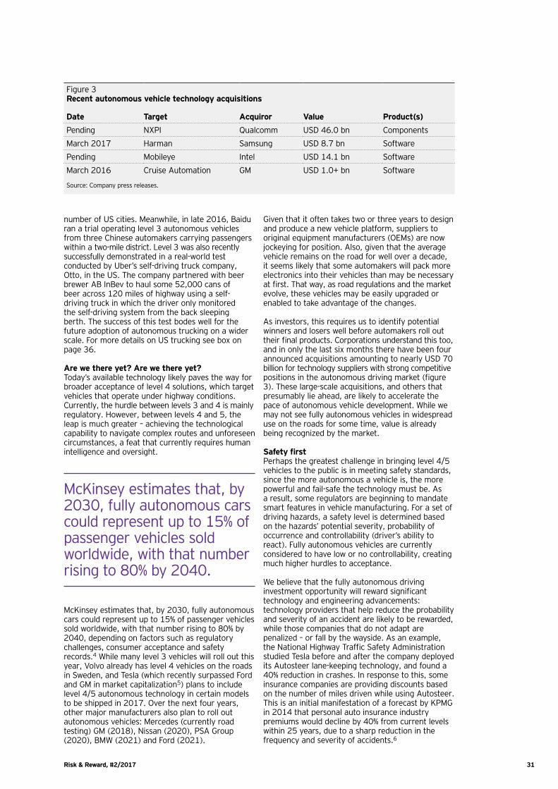
Risk & Reward, #2/2017 31
number of US cities. Meanwhile, in late 2016, Baidu ran a trial operating level 3 autonomous vehicles from three Chinese automakers carrying passengers within a two-mile district. Level 3 was also recently successfully demonstrated in a real-world test conducted by Uber’s self-driving truck company, Otto, in the US. The company partnered with beer brewer AB InBev to haul some 52,000 cans of beer across 120 miles of highway using a self- driving truck in which the driver only monitored the self-driving system from the back sleeping berth. The success of this test bodes well for the future adoption of autonomous trucking on a wider scale. For more details on US trucking see box on page 36.
Are we there yet? Are we there yet? Today’s available technology likely paves the way for broader acceptance of level 4 solutions, which target vehicles that operate under highway conditions. Currently, the hurdle between levels 3 and 4 is mainly regulatory. However, between levels 4 and 5, the leap is much greater — achieving the technological capability to navigate complex routes and unforeseen circumstances, a feat that currently requires human intelligence and oversight.
Given that it often takes two or three years to design and produce a new vehicle platform, suppliers to original equipment manufacturers (OEMs) are now jockeying for position. Also, given that the average vehicle remains on the road for well over a decade, it seems likely that some automakers will pack more electronics into their vehicles than may be necessary at first. That way, as road regulations and the market evolve, these vehicles may be easily upgraded or enabled to take advantage of the changes.
As investors, this requires us to identify potential winners and losers well before automakers roll out their final products. Corporations understand this too, and in only the last six months there have been four announced acquisitions amounting to nearly USD 70 billion for technology suppliers with strong competitive positions in the autonomous driving market (figure 3). These large-scale acquisitions, and others that presumably lie ahead, are likely to accelerate the pace of autonomous vehicle development. While we may not see fully autonomous vehicles in widespread use on the roads for some time, value is already being recognized by the market.
Safety firstPerhaps the greatest challenge in bringing level 4/5 vehicles to the public is in meeting safety standards, since the more autonomous a vehicle is, the more powerful and fail-safe the technology must be. As a result, some regulators are beginning to mandate smart features in vehicle manufacturing. For a set of driving hazards, a safety level is determined based on the hazards’ potential severity, probability of occurrence and controllability (driver’s ability to react). Fully autonomous vehicles are currently considered to have low or no controllability, creating much higher hurdles to acceptance.
We believe that the fully autonomous driving investment opportunity will reward significant technology and engineering advancements: technology providers that help reduce the probability and severity of an accident are likely to be rewarded, while those companies that do not adapt are penalized – or fall by the wayside. As an example, the National Highway Traffic Safety Administration studied Tesla before and after the company deployed its Autosteer lane-keeping technology, and found a 40% reduction in crashes. In response to this, some insurance companies are providing discounts based on the number of miles driven while using Autosteer. This is an initial manifestation of a forecast by KPMG in 2014 that personal auto insurance industry premiums would decline by 40% from current levels within 25 years, due to a sharp reduction in the frequency and severity of accidents.6
Figure 3Recent autonomous vehicle technology acquisitions
Date Target Acquiror Value Product(s)
Pending NXPI Qualcomm USD 46.0 bn Components
March 2017 Harman Samsung USD 8.7 bn Software
Pending Mobileye Intel USD 14.1 bn Software
March 2016 Cruise Automation GM USD 1.0+ bn Software
Source: Company press releases.
McKinsey estimates that, by 2030, fully autonomous cars could represent up to 15% of passenger vehicles sold worldwide, with that number rising to 80% by 2040.
McKinsey estimates that, by 2030, fully autonomous cars could represent up to 15% of passenger vehicles sold worldwide, with that number rising to 80% by 2040, depending on factors such as regulatory challenges, consumer acceptance and safety records.4 While many level 3 vehicles will roll out this year, Volvo already has level 4 vehicles on the roads in Sweden, and Tesla (which recently surpassed Ford and GM in market capitalization5) plans to include level 4/5 autonomous technology in certain models to be shipped in 2017. Over the next four years, other major manufacturers also plan to roll out autonomous vehicles: Mercedes (currently road testing) GM (2018), Nissan (2020), PSA Group (2020), BMW (2021) and Ford (2021).

Risk & Reward, #2/2017 32
Greater complexity = greater opportunityThe US experienced approximately 40,000 road fatalities in 2016, with an additional 4.6 million people injured and associated costs estimated at a staggering USD 432 billion.7 Most of these accidents were caused by driver error. With economic incentives to automate driving already becoming apparent, the push forward to achieve higher levels of autonomy should generate even more interest. The volume of electronics in a vehicle grows exponentially as the level of autonomy increases, providing a significant growth opportunity for technology companies with the right products. For example, to achieve level 2 autonomy, a vehicle needs four specific sensors – but that requirement doubles to achieve level 3. Achieving level 4/5 autonomy necessitates up to 21 sensors to create a road and hazard-monitoring cocoon around a vehicle (figure 4). The sensor dollar content opportunity alone increases from USD 35 per vehicle at level 1 to USD 325 per vehicle at level 4, a more than 9x increase for technology providers.8
Level 4/5 autonomy will require an increasingly powerful chip to process the huge quantities of data generated by these sensors and to make decisions on changes to a vehicle’s actions. Furthermore, separate chips will be needed to control the physical movements of the vehicle. Autonomous driving is pushing research, development and consolidation in the chip sector much like internet gaming did approximately a decade earlier.
Autonomous vehicles will also require microphones for voice commands, chips to permit communication with other vehicles and objects, and more. We estimate that additional components will go from USD 20 per level 1 vehicle to USD 370 in a level 4 vehicle. Mapping software and software algorithms that provide the intelligence to power the chips will become competitive differentiators, as will the vast quantities of data (collected from real-world driving
experience) that are used to train the software to do its job well. Ford recently announced that it would invest USD 200 million to build a new data centre to house consumer information associated with connected and autonomous vehicles.
The autonomous vehicle opportunity is considered to be strategically important for a large and diverse set of incumbents, including technology companies (e.g., Google, Uber, Baidu and Nvidia), automobile manufacturers (e.g., GM, Ford, Tesla and Toyota) and OEMs. Creating autonomous vehicles is also a capital- and labour-intensive process in a very heavily regulated industry. In other areas of technological disruption, where the product and challenge is software-based, start-ups can leverage cloud computing and storage to build and release a product on more limited capital. With autonomous vehicles, the challenges are rooted in hardware and regulatory dynamics that inevitably require more capital investment, limiting participation by companies that are not well-capitalized. Moreover, sensor, mapping and vehicle usage data will provide a moat and competitive advantage for incumbents like Uber, Lyft and Didi (China’s largest ride-sharing service), creating a barrier to entry for start-ups looking to tackle autonomous vehicles head on. Therefore, the core self-driving opportunity may be more challenging than usual for start-ups to pursue. As a result, many start-ups are focusing on niche, enabling or derivative opportunities stemming from an autonomous world. Start-ups with a head start quickly become acquisition or investment candidates for strategic players keen not to get left behind. GM bought the self-driving technology start-up Cruise Automation last year, while Ford purchased the ride-sharing service Chariot, and more recently committed to invest USD 1 billion in the Pittsburgh-based Argo AI to both expedite Ford's ability to get a self-driving car to market as well as potentially licence the technology to others. Thus, incumbent (public and private) technology and automobile companies will in our
Figure 4More sensors required for each automation level
• Radar • Camera • Lidar
2015 Euro-NCAP*
2018 Euro-NCAP*
Level 2 Level 3 Level 4/5
Front looking camera 0.5 1 1 1 1
Front looking radar 0.5 1 1 1 1
Front looking lidar – – – – 1
Surround camera – – – – 4
Corner radar – 2 2 4 4
Surround radar – – – – 6
Rear looking camera – – – 1 1
Rear looking radar – – – – 1
Driver monitoring camera – – – 1 1
Vehicle-to-X sensor – – – – 1
Parking aid Up to 12 ultrasonic sensors per car
Automated parking Potential future replacement by RF CMOS** radar
* Euro-NCAP (European New Car Assessment Programme) is focusing on collision avoidance, requirements are increasing over time.** RF CMOS = Radio-Frequency Complementary Metal-Oxide Semi-Conductor.Source: Infineon Technologies AG, as at 2 August 2016. The information may change due to technical progress.

Risk & Reward, #2/2017 33
view significantly drive the adoption of autonomous vehicles, but new entrants will contribute throughout the value chain.
As noted above, safety regulations pose a significant near-term challenge to getting fully autonomous vehicles on the road in non-controlled settings. A number of start-ups are addressing this intermediate step. ZenDrive focuses on the overall safety of the driving ecosystem, utilizing smartphone sensors to deliver safety insights to fleet owners and other enterprise customers. Nauto, meanwhile, designs artificial intelligence for collision avoidance, but with an aftermarket component add-on that collects and processes visual data. Rather than functioning as a core-autonomous vehicle company, Nauto is more focused on upgrading existing connected cars. INRIX is focused on the safety and traffic implications of accidents, leveraging real-time, predictive data analytics for traffic and mapping.
Companies that provide the components required for technological upgrades can benefit as consumers increasingly demand safety features that reduce their risk and can lower their insurance bills. Many start-ups and venture capitalists have also identified enabling technologies, like computer vision and user-generated mapping, as areas where they can facilitate the development of autonomous vehicles. Navigation (including understanding signage) and mapping are necessary for building the autonomous vehicle operating system and artificial intelligence training, as autonomous vehicles require much greater detail than pedestrians. Google’s self-driving car division, Waymo, has been engaged in a whole new level of mapping the world, including “the height of a curb, the width of an intersection and the exact location of a traffic light or stop sign.”9
Computer vision has many applications, but is of growing importance to autonomous vehicles in mapping environments accurate to the nearest centimetre, as well as avoiding pedestrians and other vehicles. Increasingly, manufacturers are planning for a future in which mapping and obstacle detection and avoidance are driven by computer vision in addition to LIDAR sensors. Tesla recently stripped out Mobileye technology from its vehicles and built its own camera-based system, leveraging ultrasonic and radar sensors. A Nokia spinout company backed by BMW, Daimler and Audi (named Here) is focused on mapping roads in the US and Europe, using a combination of sensors and computer vision. The company, which last year announced a partnership with Mobileye, relies on a combination of data from scanning systems installed in trucks, alongside its own image-collecting fleet. The data is then annotated (manually or by computer) to produce the maps. In a similar vein, Mapillary is a service for crowdsourcing street-view photographs and matching them across time and location, leveraging computer vision. Mapillary uses machine learning to sort through its vast database of street-view photos and identify those most relevant to autonomous vehicles, which the company then sells to manufacturers. Computer vision and navigation may not create large, stand-alone public companies, but are crucial enabling technologies, and could spawn companies that will help shape the development of autonomous vehicles and become prime candidates for strategic acquisition.
At the same time, there are others building the full autonomous kit (both hardware and software) to sell to car manufacturers or aiming to create full autonomous vehicles themselves. Aurora Innovation, founded by former Alphabet self-driving guru Chris Urmson, is in stealth mode, but is reportedly taking the former approach. Similarly, Drive.ai adopting a more holistic approach, using deep learning throughout instead of manually creating rules to help algorithms identify objects. On the service side, Zoox has raised almost USD 300 million, at a USD 1.5 billion valuation, to create a fleet of autonomous vehicles for the purpose of mobility- as-a-service – competing with the likes of Uber and Didi. While these players will likely see outcomes further down the road than the smaller niche players discussed above, they have the potential to become either strategic partnerships for other more vertically focused solutions or, eventually, acquisition targets for large autonomous vehicle incumbents.
While there are certainly a significant number of new entrants raising large sums of money to address the opportunity of manufacturing and selling autonomous vehicles, others are taking a leaner approach that focuses on getting vehicles into market more quickly and cheaply. Some companies are targeting lower-hanging fruits by getting products that are not fully autonomous into the market, while others are focusing on rolling out slow-to-moderate moving vehicles on private roads (e.g. private developments and college or corporate campuses), where the regulatory hurdles are not as significant. Optimus Ride and nuTonomy are taking this approach. Meanwhile Comma.ai, similar to Nauto, is focused on retrofitting existing vehicles using off-the-shelf components, while open-sourcing the data from its driverless trips.
Wider implicationsThe early winners in the shift toward autonomous driving are likely to be technology providers. This could create opportunities in the semiconductor, software, audio visual and radar technology areas that make autonomous driving possible. However, as mentioned above, there will likely be losers too: figure 5 provides a sense of the enormous range of driver-dependent industries likely to be impacted. As the responsibility for driving shifts from individuals to technology companies and vehicle manufacturers, we are likely to see a significant impact on these firms’ economic and business models.
The rise of autonomous vehicles may also disrupt the property and casualty insurance market, as auto insurance is currently this market’s largest, most profitable segment. It could have a critical impact as this industry has been saddled with losses due to substantial decreases in premiums; insurers will also need to adjust their loss risk models significantly over time. If accident rates between human drivers and autonomous vehicles are sufficiently different, it may actually become illegal at some point to drive cars personally.
In the intermediate term, the cost to insure a vehicle may actually increase as loss severity (the cost to fix the vehicle) moves higher due to the increased dollar content of the components and software featured in newer autonomous vehicles. However, longer term,

Risk & Reward, #2/2017 34
we would expect the frequency of accidents to decline, which should reduce industry loss costs and, ultimately, premiums. The impact of this trend is already being felt, as some insurers with significant auto underwriting exposure are expanding into new business lines in order to remain relevant to the consumer.
If autonomous vehicles become omnipresent, this could also have a profound impact on real estate markets. First, it will undoubtedly change the value proposition of living in cities versus living in suburbs, given the potential significant reduction in traffic and travel times. Simultaneously, it may free up urban real estate previously occupied by curbside parking or parking lots and garages, including those at airports, as more people rely on autonomous vehicle services rather than driving and parking their own vehicles. These dynamics could lead to a substantial decline in urban (both commercial and residential) real estate prices.
Autonomous driving has the potential to affect a host of seemingly unrelated industries as well. Ancillary businesses are already popping up to capitalize on the new trend. For example, the online education company Udacity, which is striving to become the “University for Silicon Valley,” just launched a “self-driving car engineer nanodegree” to address the dearth of qualified deep learning engineers with autonomous vehicle experience.
The road aheadWhile, as noted earlier, 2016 saw significant advances in the development of autonomous driving hardware and related M&A activity, there are sub-segments of autonomous vehicle-enabling technology that clearly need to be developed before fully autonomous vehicles can become a day-to-day reality.10 As noted earlier, regulation may also create headwinds as governments try to ensure public safety while encouraging continued technological advancement. Moreover, the increasing prevalence of driverless vehicles and other automation technology will be accompanied by a variety of novel and difficult ethical and societal issues11, such as how to deal with the significant job losses they will cause. Finally, widespread acceptance of autonomous vehicles will depend in large part upon manufacturers’ ability to produce them at price points that are accessible to large numbers of consumers.
We will likely see waves of innovation and newer entrants focused on the development of these enabling technologies. The industry has already seen this pattern; for example, innovations in the internet of things and connected cars have paved the way for safety, communication and navigation technology that leverages the wave of newly created data. Although some of these enabling opportunities may not be as truly transformative as autonomous vehicles, they can provide lucrative and nearer-term opportunities for start-ups and venture capital. Moreover, many of these enabling and ancillary technologies can become prime acquisition candidates for strategic players in their race for autonomous primacy.
Autonomy could ultimately provide an additional boon to car manufacturers, as it represents a step change in functionality that – combined with greater
individual car utilization – may cause the upgrade/replacement cycle to abbreviate, akin to the phone or laptop. It could also modularize and lead to prioritization of different features across models. The “car as a platform” would also create many derivative opportunities and challenges necessitating the creation of relevant applications and cybersecurity.
It is possible that autonomous vehicle manufacturers will shift from a business-to-consumer to a business-to-business model as personal car ownership declines, which may ultimately result in consumers interacting with fleet operators as they currently do with air travel. This could happen not only for cars, but for other vehicles as well. For example, NEXT Future Transportation is already building modular autonomous bus systems focused both on highways and last-mile transport. Fully autonomous vehicle fleets could ultimately function like a city bike-share programme, or perhaps even as a public utility, enabled by fleet optimization software and car-to-car communication capabilities. The latter may also involve a machine-to-machine payment system utilizing blockchain-based tokens like bitcoin (e.g., a driver in a rush makes a payment to other cars to move out of the way). Blockchain and bitcoin have long been transformative technologies in search of “killer applications” or use cases, and an automated world could finally provide this.
ConclusionWhen assessing the investment implications of autonomous vehicles, new opportunities within the automotive, transportation and technology industries spring immediately to investors’ minds. However, it is important to also keep other ramifications in mind
Figure 5Industries impacted by the shift to autonomous driving
Auto repair Collision repair is a USD 30 bn industry
Medical USD 23 bn in medical expenses due to vehicle crashes
Auto insurance USD 220 bn in annual policy premiums
Municipalities Reduced traffic violation revenues
Legal profession 76,000 personal injury attorneys in the US
Construction Less parking; lane design changes
Digital media Benefits from “free time” in vehicles
Oil & gas 20-30% decrease in demand
Source: Department of Transportation, McKinsey, KPMG 2015. Economic Effects of Automated Vehicles, Lewis Clements, Kara Kockelman January 2017.

Risk & Reward, #2/2017 35
About the authors
Jim ColquittAnalyst, Invesco Fixed IncomeJim Colquitt is an analyst with the Invesco Fixed Income High Yield team, with researchresponsibilities for gaming, leisure, lodging and telecommunications.
Dave Dowsett Global Head of Invesco’s Innovation, Strategy and Disruptive Technology teamDave Dowsett is Global Head of Invesco’s Innovation, Strategy and Disruptive Technology team, which focuses on augmenting Invesco’s technology strategy with the newest financial technology in development in the marketplace.
Abhishek GamiSenior Equities Analyst, Invesco Fundamental EquitiesAbhishek Gami is a Senior Equities Analyst working with the Large/Multi-Cap Growth team.
Evan Jaysane-DarrPartner, Invesco Private CapitalEvan Darr is a Portfolio Manager with Invesco Private Capital (IPC), making direct company and partnership investments into venture capital and private equity on behalf of IPC’s institutional and high net worth clients.
Clay ManleyPortfolio Manager, Invesco Fundamental EquityClay Manley is responsible for the management of Small Cap Growth portfolios.
Rahim ShadSenior Analyst – High Yield, Invesco Fixed IncomeRahim Shad is a Senior Analyst for Invesco Fixed Income. He has research responsibilities for metals and mining, media and technology.
Notes1 “How do driverless cars work?”, The Telegraph, 1 July 2016.2 In 2016, a computer defeated human opponents to become the
world champion at Go, a complex strategy game involving an almost infinite number of potential opponent moves. In 2017 researchers at Carnegie Mellon and the University of Alberta are testing their artificial intelligence talent in the No-Limit Texas Hold ‘Em poker competition, where computers encounter not only the unknowns associated with multiple card decks, but also the irrationality of the human mind and opponents who may be purposely providing misleading information by bluffing.
3 Light Detection and Ranging, a system similar to radar using light pulses rather than sound waves.
4 McKinsey & Company, “Disruptive trends that will transform the auto industry”, January 2016.
5 Wall Street Journal, “Tesla, on a Hot Streak, Passes Ford in Investor Value”, April 3, 2017.
6 KPMG, “Marketplace of Change: Automobile insurance in the era of autonomous vehicles” October 2015.
7 Fortune, “2016 was the deadliest year on American roads in a decade”. February 15, 2017.
8 Chris J . Needham, “Artificial Intelligence: The Road to Human Inference”, December 2016.
9 “Building Maps for a Self-Driving Car”, Medium 2016.10 Tesla began outfitting its vehicles in 2016 with fully autonomous
driving hardware, which will be supplemented by means of automatic software updates as related technology continues to advance.
11 For instance, the guidance software for an autonomous vehicle may need to determine whether to swerve into a pedestrian in order to avoid a head-on collision with another vehicle.
When assessing the investment implications of autonomous vehicles, new opportunities within the automotive, transportation and technology industries spring immediately to investors’ minds.
that may not be as readily apparent: Real estate portfolios could be affected by shifts in residential and commercial demand patterns driven by changing to commute times and parking needs. Financial services providers could be impacted by new types of insurance policies or a move away from widespread vehicle ownership. The list of winners and losers in the driverless vehicle era will continue to evolve rapidly, just as the investment landscape did with the rapid growth of personal computing, internet retailing and other transformational trends. It will therefore be critical to anticipate, analyze and adapt to these changes, something that active managers like Invesco do every day, in order to identify and act upon tomorrow’s investment opportunities, today.

Risk & Reward, #2/2017 36
Box Keep on truckin’ Approximately 70% of all freight tonnage in the US is moved via trucks, so there are clear benefits to making this process more efficient and less costly, particularly for long-haul routes. Autonomous trucking has seen innovation come principally from start-ups. While it is a less universal market opportunity than self-driving cars, trucking may represent a nearer-term one for smaller companies since there are fewer well-capitalized or technology-focused incumbents focused on this space and long-haul routes present fewer technical challenges than city driving.
Uber bought self-driving truck company Otto for USD 680 million, plus 20% of future self-driving profits.* But Otto is not without competition. Peloton has focused on the intermediate step toward fully autonomous vehicles, creating a technology that allows trucks to travel in fleets, thereby reducing the need for driver control. Silicon Valley-based Embark has developed software enabling trucks to drive “exit to exit” on the highway without any human assistance.
Trucking’s inherent challenges present opportunity for autonomous vehiclesA number of issues faced by the trucking industry make it an excellent candidate for autonomous innovation. According to the American Transport Research Institute,** the industry’s key challenges include:
• Driver fatigue While completely replacing drivers is still years away, extending the service hours of a truck by making it autonomous is a nearer-term possibility. Current regulations mandate a 14-hour on-duty limit for truck drivers, of which only 11 hours can be spent driving. The industry already suffers from a shortage of drivers as well as retention issues. Autonomous driving technology could certainly help address these points. Even at level 4, on-road hours could be extended and more drivers could be potentially moved into “supervisory” roles.
• Safety and human error As noted earlier, the overwhelming majority of traffic accidents are caused by human error and could potentially be avoided with advanced collision prevention technologies. As trucking automation progresses, among the important developments to watch will be technology that enables autonomous city driving, which involves the ability to follow complex traffic rules and detect unexpected traffic situations, such as crossing pedestrians.
• Need for infrastructure upgrade Because autonomous vehicles require properly maintained infrastructure to operate well, US infrastructure will need to be significantly upgraded to enable full scale adoption of this technology. For example, vehicles must be able to read lane markings and speed limits. It is worth noting in this regard that infrastructure improvements appear to be among the Trump administration’s top policy priorities in the US. Autonomous driving technology could also provide a more efficient way to deal with congestion through lane and space management and could potentially optimize trucking routes as well.
• Economics and cost efficiency As noted above, the trucking industry plays a large role in the US economy, and there are clear benefits to making the process of transporting freight more efficient. The easy gains can be made through the extension of service hours, fewer interruptions and improved routes. If the goal is to get a truckload of products from point A to point B, autonomous driving promises to do it more efficiently, safely and cheaply than human-directed driving. The cost breakdown of a trucking assignment shows that roughly two-thirds of the operational costs are related to driver compensation and fuel, as seen in the figure below. level 5 trucks would eliminate the personnel expense entirely, and even level 4 (driver present) could provide economic benefits. Additional benefits would likely derive from efficiency gains. For example, trucks operated in an autonomous fashion could potentially drive more closely together and maintain steadier speeds, thereby generating significant fuel economies. According to the Otto study, even with a driver present, autonomous driving was estimated to potentially save AB InBev USD 50 million per year in operating costs through reduced fuel expense and frequent delivery schedules.***
US trucking industry
Quick facts Challenges
Moves 70% of US freight
Labour: 30% of trucking costs
15 million operational trucks
Fuel: 40% of trucking costs
Mostly interstate highway driving
Scheduling, inefficient routing
Source: American Trucking Association, Auburn University, Roland Berger 2016. “Autonomous and Self-Driving Trucks will Improve Safety, Fuel Economy”, Trucks.com, 7 April 2016.
* Source: “Otto hauls Budweiser in First Commercial Use of Self-Driving Truck”, Trucks.com, 25 October 2016. ** Source: American Transport Research Institute, November 2016. *** Source: Bloomberg L.P., 25 October 2016.

Risk & Reward, #2/2017 37
In briefAt this year’s Cambridge Investment Lectures, three leading experts from the University of Cambridge Judge Business School shared their insights on current investment topics. Raghavendra Rau expects a rapid evolution of alternative financing, also as an asset class; Elroy Dimson talked about return expectations and stressed the potential portfolio impact of factor exposures; Peter Williamson highlighted what investors should pay attention to in China.
The 2017 Cambridge Investment Lectures
On 28 February 2017, Invesco’s Cambridge Investment Lectures brought together the latest investment insights from three leading members of the faculty of the University of Cambridge Judge Business School. At King’s College, Cambridge, Raghavendra Rau, Elroy Dimson and Peter Williamson presented their views to Invesco clients. The three professors talked about alternative finance, global investing and opportunities in China.
Raghavendra Rau: Is alternative finance an alternative asset class?The event began with a presentation by Raghavendra Rau, Sir Evelyn de Rothschild Professor of Finance, and a leading expert on alternative finance. Professor Rau stressed that “alternative finance” is not to be confused with “alternative investing”, even though alternative finance also offers a range of investment opportunities.
Indeed, there are various types of alternative finance: crowdfunding, peer-to-peer lending, mobile payment systems (such as mPesa), direct issue bonds, wealth advisory systems (so-called robo-advisors), alternatives to foreign exchange and traditional payments systems, as well as Bitcoin and other distributed ledger systems – to name just a few. Professor Rau estimates that the global volume traded on alternative finance platforms has risen sharply, to USD 147 billion in 2015 from USD 14 billion in 2013 (and only USD 0.5 billion in 2011).
In order to assess whether alternative finance is an alternative asset class, Professor Rau identified the four key characteristics of an investable asset class. First, the market for the asset should be understandable. Second, it should be broad – either geographically and/or across industries. Third, it should be deep, so it is easy to enter and exit. Fourth, correlation with existing assets should be low.
To what extent do these new alternative finance platforms meet these four requirements, Professor Rau asked – and answered one by one.
Is the market understandable?In Professor Rau’s view, new forms and sources of data mean that problems of asymmetric information are reduced and human behaviour becomes easier to assess and predict. Harnessing social media data, including the use of geospatial information, is an important aspect of this development. We now have much richer sources of information to help understand human behaviour.King’s College, Cambridge

Risk & Reward, #2/2017 38
Is the market broad?The alternative finance market is indeed broad, in that it is diversified geographically and across industries, Professor Rau continued. Globally, in 2016, there were 1,362 alternative finance platforms in 153 countries.1 Geographically, the US, UK and China have the best-developed alternative finance markets relative to GDP (figure 1). China alone has more than 400 alternative finance platforms.
But alternative finance can take many forms, and Professor Rau set out a general typology of crowdfunding models (figure 2), with examples in each of the different categories. The peer-to-peer (P2P) lending category is by far the largest in terms of volume, and provides the most direct alternative to traditional bank financing. In a recent survey, 79% of borrowers in the P2P market had sought funding from banks (but only 22% had received an offer) before turning to the P2P market. The majority of
companies accessing the market had been trading for more than 10 years, with annual turnover in the range of GBP 200,000-500,000, and typically borrowed GBP 1,000-5,000.2
The P2P business model is generally based on less costly loan origination compared to the banks (notably because P2P lenders do not have the cost of a branch network), faster and more accurate credit scoring, and lower compliance costs due to a lower regulatory burden. Interestingly, as Professor Rau pointed out, there is evidence that banks’ inclination to lend increases after a company has received platform funding.
Is the market sufficiently deep? To answer the third question, Professor Rau cited a recent deal by the UK Universities Superannuation Scheme (USS) and Credit Suisse as evidence of market depth. Credit Suisse agreed to offload most of a portfolio of loans and loan commitments made in 2014 and 2015, typically lasting five to seven years, to USS. The bank, which retained a small portion of the original lending, will manage the pool of loans and arrange new financing for USS on the same basis.
Low correlation with traditional assetsFinally, as the market is still in its early stages, there are, of course, risks involved. Professor Rau pointed out that it is too early as yet to fully understand the correlation between returns in the alternative finance market and those in traditional markets. However, he mentioned that the Cambridge Centre for Alternative Finance is working with the UK’s Financial Conduct Authority as it looks more closely at regulatory issues facing the sector.3
Figure 1Alternative finance vs. GDPAlternative finance volume per capita vs. GDP per capita, 2015
Volume/capita (log), USD
0.00
0.01
0.10
1.00
10
100
1000
0 10 20 30 40 50 60 70
ChinaUK US
GDP/capita (USD, 000s)
Source: Cambridge Centre for Alternative Finance. Data as at 28 February 2017.
Figure 2A general typology of crowdfunding models
Forms of contribution Forms of return Motivation of funder
Debt-based crowdfunding/P2P lending
Loan (secured or non-secured)
Repayment of loan (with or without interest)
Primarily financially driven but can also be for altruistic reasons
Equity-based crowdfunding
Investment Financial or material rewards during exit/profit sharing
Primarily financially driven/combination of reasons
Reward-based crowdfunding
Donation/pre-sell Material/non-financial rewards and tangible benefits
Combination of intrinsic, social motives as well as rewards
Donation-based crowdfunding
Donation Non-financial and intangible benefits
Intrinsic, social and affinity-based motivations
Source: Cambridge Centre for Alternative Finance. Data as at 28 February 2017.
“The alternative finance market satisfies many of the characteristics of an investable asset class, and can be expected to continue a rapid evolution.” Raghavendra Rau

Risk & Reward, #2/2017 39
Professor Rau concluded by drawing attention to the alternative finance market’s rapid development. Traditional finance models, he said, had been challenged in many different areas. Or, in his own words: “The alternative finance market satisfies many of the characteristics of an investable asset class, and can be expected to continue a rapid evolution.”
Elroy Dimson: Global investing – a historical and forward-looking perspectiveThe second talk of the day featured Professor Elroy Dimson from the Cambridge Judge Business School. As chairman of the Strategy Council for the Norwegian Government Pension Fund, he is a renowned expert on global investing. In his lecture, he first looked at the past, present and future of global financial market returns, and then considered whether factor investing was indeed “smart”.
Global returns: the past …Professor Dimson referred to the Dimson, Marsh and Staunton (DMS) data (first presented publicly in 2002 in the book “Triumph of the Optimists”), which Dimson co-authored.4 Since then, the data has been updated annually. Today, it covers 23 countries with 21 unbroken histories over a period of 117 years, from the start of 1900 to the end of 2016.
Professor Dimson gave a striking example: in the US market, one US dollar invested in equities on 1 January 1900 would have grown, with all dividends reinvested, to USD 1,402 in real terms by the end of 2016 – for a compound average return of 6.4% p.a.
In contrast, one US dollar invested in US corporate bonds, with all income reinvested, would have grown to just USD 11.90 in real terms, with a compound average return of 2.0% p.a. – similar to the capital-only average return from US equities over the same period. So, the real return premium of equities over bonds in this long-term context was largely due to the reinvestment of dividends.
For completeness, Professor Dimson added that the 6.4% p.a. real return from US equities over that period was higher than in all the other 22 markets in the study, apart from Australia and South Africa. The average real return from the non-US countries was 4.3% p.a. and for the world in total 5.1% p.a. That meant the 117-year average world equity risk premium over bonds was 3.2% p.a. and relative to Treasury bills 4.2% p.a.
… the present …When looking at the future real returns on bonds, there is no need to extrapolate past returns: they can be directly observed from the index-linked bond market. At present, average 10-year real yields in the seven major markets where such instruments exist (US, UK, France, Germany, Japan, Canada and Sweden) were around minus 0.5% at the end of February 2017, Professor Dimson said. That is very different from the situation at the turn of the millennium, when the average was a positive 3.5%-4%. Some claim that, in a low real interest rate environment, it is necessary to invest in equities to generate a higher real return. But
over the 2,317 country years of data available for analysis, Professor Dimson found that low real interest rates are associated with low real bond and equity returns in the subsequent five years. “Equities do not escape the effect of low real interest rates”, Dimson concluded.
… and the futureSo, what does the future hold for equity risk premiums? The historic average world real equity return of 5.1% p.a. comprises a 4.1% average dividend yield and 0.5% from each of two other factors: real dividend growth and a change in the price/dividend ratio (figure 3). Those latter two factors are unlikely to be repeated in the future – and so it is prudent to exclude them from future return estimates. So, given an expected real Treasury bill return of 0.8% p.a., Professor Dimson estimated that a 3-3.5% long-run equity risk premium relative to bills can be expected for the future. That is lower than the historical average of 4.2%.
Factor investing: is it smart?In the second part of his talk, Professor Dimson turned to factor investing. He stressed that, in today’s low return world, the current vogue is to seek returns from factor or “smart beta” strategies.
There has been rapid growth in “smart beta” assets under management, from USD 200 billion at the end of 2012 to over USD 500 billion at the end of 2016.5 Researchers have reported on as many as 458 factors that have been associated with superior returns. This, Professor Dimson said, is a huge increase from the standard three-factor model (market risk, size and value) or the five-factor (including profitability and investment) model – both developed by Fama and French.6 Others, Professor Dimson went on, have stressed the importance of low-risk and momentum.
Figure 3What equity premium can we expect in the future?
Annualized (% p.a.)
5.1 0.5
0.5
4.1 0.8
3.3
Historicalequity real return
Realdividendgrowth
Changein P/Dratio
Averagedividendyield
Treasurybill return
Expectedriskpremium
0
1
2
3
4
5
6
Source: Elroy Dimson, Paul Marsh and Mike Staunton. Data as at 28 February 2017. Forecasts are based upon current market conditions and are subject to change without notice.

Risk & Reward, #2/2017 40
Professor Dimson, together with two colleagues,7
had looked at the behaviour of five factors: low-risk, momentum, size, value and income in the US and UK equity markets from 2008-2016 (figure 4). He talked about each of these factors in turn.
Low riskLow-risk investing is the “classic” factor strategy, first identified by Fischer Black in 1972.8 He showed that a US low-beta portfolio gave superior risk-adjusted returns compared with a high-beta strategy. This is now referred to as the BAB (Bet Against Beta) strategy. Recent research has developed the work to use different measures of volatility. Looking at three different variants – the traditional approach, i.e. low versus high beta stocks, as well as low versus high variance stocks and low versus high specific risk stocks – Professor Dimson and his colleagues Marsh and Staunton found that globally, the weakest effect was BAB, and the strongest effect was favouring stocks with low specific risk over those with high specific risk.
MomentumA momentum strategy sorts stocks according to their returns over the previous 6 or 12 months. The top and bottom ranked stocks (typically by quintile) are selected. The strategy is to buy past winners and short past losers, implemented after a one month lag. The portfolio is rebalanced periodically.
The momentum premium is found to be large, before trading costs are taken into account: 7.4% p.a. in the US (from 1926-2016) and 10.4% p.a. in the UK (from 1900-2016). The returns from the strategy, however, are volatile, and turnover is high. Momentum returns have been identified around the world: they were found in an initial study using data to the end of
20009, and Professor Dimson found this effect to be larger when subsequent years (to the end of 2016) are added. His work shows an average global premium of winners minus losers of about ¾% per month.
Size, value and incomeThree other factors: size (small stocks perform better than large stocks), value (high book-to-market stocks perform better than low book-to-market stocks) and income (high yield stocks produce higher returns than low yield stocks), were all found to exist in the US, UK and most countries in the long-term data according to the Dimson, Marsh and Staunton research.10
Professor Dimson concluded that it is important to distinguish between factors – i.e. influences on asset returns – and premiums – i.e. the superior returns expected from those factors. Premiums may be evident over the long-run, and in some cases can be harvested passively; others vary over time and across markets, and may require extensive portfolio rebalancing. There is no doubt that factor exposures can have a large performance impact and investors may sometimes unwittingly take large bets. Furthermore, factors can become too expensive, as their popularity can make them an over-crowded trade. Prudent investors should therefore consider diversifying across multiple factor-investing strategies.
Figure 4Factor performance since the financial crisis
2008 2009 2010 2011 2012 2013 2014 2015 2016 2008-16Highest
Highest
Lowest
Lowest
US
UK
Low vol90.3
Low vol127.0
Low vol-22.9
Low vol-15.2
Income20.7
Income15.7
Income-13.7
Income7.1
Momentum-2.4
Momentum78.8
Momentum0.7
Momentum8.5
Size-4.3
Size-17.5
Size12.4
Size13.6
Value-6.0
Value-11.8
Value3.2
Low vol-20.1
Low vol-33.0
Income1.1
Income-17.2
Momentum-25.4
Momentum-50.6
Size24.9
Size28.5
Value-6.9
Value-8.0
Value-4.5
Low vol35.0
Low vol40.5
Income28.3
Income29.5
Momentum20.6
Momentum1.4
Size-4.9
Size-3.7
Value-10.7
Value-12.8
Low vol-15.7
Low vol-1.5
Income-8.1
Income-7.6
Momentum-1.7
Momentum-0.9
Size17.0
Size7.8
Value14.8
Value11.5
Low vol11.5
Low vol-9.3
Income0.0
Income-8.2
Momentum32.4
Momentum4.5
Size15.5
Size5.3
Value0.0
Value4.7
Low vol-6.2
Low vol11.3
Income-1.3
Income1.6
Momentum42.8
Momentum-5.3
Size12.1
Size-6.7
Value-10.0
Value-2.2
Low vol23.7
Low vol13.9
Income-11.2
Income2.4
Momentum20.1
Momentum42.3
Size11.1
Size-9.3
Value-20.9
Value-12.0
Low vol-21.2
Low vol-1.8
Income15.3
Income14.8
Momentum-18.3
Momentum-22.4
Size-4.9
Size9.6
Value20.2
Value17.2
Low vol5.5
Low vol6.0
Income2.1
Income3.8
Momentum12.8
Momentum-6.0
Size6.5
Size4.0
Value-3.2
Value-1.8
Source: Cambridge Centre for Alternative Finance. Data as at 28 February 2017.
“There is no doubt that factor exposures can have a large performance impact.” Elroy Dimson
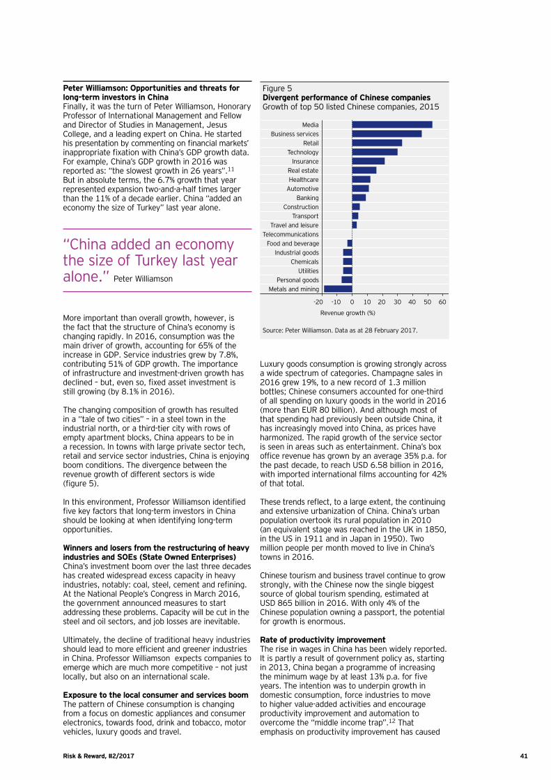
Risk & Reward, #2/2017 41
Peter Williamson: Opportunities and threats for long-term investors in ChinaFinally, it was the turn of Peter Williamson, Honorary Professor of International Management and Fellow and Director of Studies in Management, Jesus College, and a leading expert on China. He started his presentation by commenting on financial markets’ inappropriate fixation with China’s GDP growth data. For example, China’s GDP growth in 2016 was reported as: “the slowest growth in 26 years”.11 But in absolute terms, the 6.7% growth that year represented expansion two-and-a-half times larger than the 11% of a decade earlier. China “added an economy the size of Turkey” last year alone.
Luxury goods consumption is growing strongly across a wide spectrum of categories. Champagne sales in 2016 grew 19%, to a new record of 1.3 million bottles; Chinese consumers accounted for one-third of all spending on luxury goods in the world in 2016 (more than EUR 80 billion). And although most of that spending had previously been outside China, it has increasingly moved into China, as prices have harmonized. The rapid growth of the service sector is seen in areas such as entertainment. China’s box office revenue has grown by an average 35% p.a. for the past decade, to reach USD 6.58 billion in 2016, with imported international films accounting for 42% of that total.
These trends reflect, to a large extent, the continuing and extensive urbanization of China. China’s urban population overtook its rural population in 2010 (an equivalent stage was reached in the UK in 1850, in the US in 1911 and in Japan in 1950). Two million people per month moved to live in China’s towns in 2016.
Chinese tourism and business travel continue to grow strongly, with the Chinese now the single biggest source of global tourism spending, estimated at USD 865 billion in 2016. With only 4% of the Chinese population owning a passport, the potential for growth is enormous.
Rate of productivity improvementThe rise in wages in China has been widely reported. It is partly a result of government policy as, starting in 2013, China began a programme of increasing the minimum wage by at least 13% p.a. for five years. The intention was to underpin growth in domestic consumption, force industries to move to higher value-added activities and encourage productivity improvement and automation to overcome the “middle income trap”.12 That emphasis on productivity improvement has caused
Figure 5Divergent performance of Chinese companies Growth of top 50 listed Chinese companies, 2015
-20 -10 0 10 20 30 40 50 60
MediaBusiness services
RetailTechnology
InsuranceReal estateHealthcare
AutomotiveBanking
ConstructionTransport
Travel and leisureTelecommunications
Food and beverageIndustrial goods
ChemicalsUtilities
Personal goodsMetals and mining
Revenue growth (%)
Source: Peter Williamson. Data as at 28 February 2017.
“China added an economy the size of Turkey last year alone.” Peter Williamson
More important than overall growth, however, is the fact that the structure of China’s economy is changing rapidly. In 2016, consumption was the main driver of growth, accounting for 65% of the increase in GDP. Service industries grew by 7.8%, contributing 51% of GDP growth. The importance of infrastructure and investment-driven growth has declined – but, even so, fixed asset investment is still growing (by 8.1% in 2016).
The changing composition of growth has resulted in a “tale of two cities” — in a steel town in the industrial north, or a third-tier city with rows of empty apartment blocks, China appears to be in a recession. In towns with large private sector tech, retail and service sector industries, China is enjoying boom conditions. The divergence between the revenue growth of different sectors is wide (figure 5).
In this environment, Professor Williamson identified five key factors that long-term investors in China should be looking at when identifying long-term opportunities.
Winners and losers from the restructuring of heavy industries and SOEs (State Owned Enterprises)China’s investment boom over the last three decades has created widespread excess capacity in heavy industries, notably: coal, steel, cement and refining. At the National People’s Congress in March 2016, the government announced measures to start addressing these problems. Capacity will be cut in the steel and oil sectors, and job losses are inevitable.
Ultimately, the decline of traditional heavy industries should lead to more efficient and greener industries in China. Professor Williamson expects companies to emerge which are much more competitive – not just locally, but also on an international scale.
Exposure to the local consumer and services boomThe pattern of Chinese consumption is changing from a focus on domestic appliances and consumer electronics, towards food, drink and tobacco, motor vehicles, luxury goods and travel.

Risk & Reward, #2/2017 42
demand for products to quadruple in the last four years, Professor Williamson concluded.
Capabilities for accelerated innovationChina is in a good position to be able to “industrialize the research and development (R&D) process”, in Professor Williamson’s view. This involves dividing the R&D process into a multitude of small steps, and putting large teams to work at each stage of the process. These teams are typically skilled technicians (of which China has many) rather than the “PhDs in white lab coats” that characterize the process in the West.
This can remove the bottlenecks created by relying on expensive, scarce equipment, and has been effective in speeding up the process of bringing new products to market. China, in Professor Williamson’s words, has also been willing to adopt the “launch-test-improve” approach to innovation: launching a basic platform before it has been fully tested, then adding functionality later.
Strategic logic of cross-border merger and acquisition (M&A) activityChinese companies’ acquisitions abroad amounted to USD 250 billion in 2016.13 Some acquisitions have clearly been ill-judged, and Professor Williamson warned of the need to steer clear of “vanity, frivolous and ‘wishful thinking’ acquisitions”. But the total included 160 relatively small deals in Europe, many of which were designed to acquire new technology – which has helped build China’s global R&D network.
In conclusion, Peter Williamson emphasized that the long-term investor should consider looking for companies that can benefit from the restructuring of heavy industries and SOEs, those with exposure to the local consumer and services boom, companies with rapidly improving productivity and rising value-added, and those with strong capabilities for accelerated innovation and the ability to take advantage of opportunities from strategic cross-border M&A, particularly in technology.
Notes1 Cambridge Centre for Alternative Finance, 2016 Report.2 Source: Cambridge Centre for Alternative Finance, data as at 28 February 2017. 3 Financial Times FCA asks University of Cambridge to help it understand P2P, 30 September
2016. https://www.ft.com/content/d5635e3a-8642-11e6-8897-2359a58ac7a54 Elroy Dimson, Paul Marsh and Mike Staunton, “Triumph of the Optimists: 101 Years of Global
Investment Returns”, Princeton University Press (2002).5 Sources: Financial Times; Morningstar Direct, as at 28 February 2017.6 Fama and French, “A Five-Factor Asset Pricing Model”, Journal of Financial Economics
(2015) 116: pp.1–22.7 Dimson, Marsh and Staunton, “Factor-based investing: The long-term evidence”, Journal of
Portfolio Management (2017 forthcoming).8 Black and Scholes, “The capital asset pricing model: some empirical tests” in: Jensen, M.C.
(Ed.), “Studies in the Theory of Capital Markets”, Praeger, New York, NY (1972).9 Griffin, Ji and Martin, “Momentum Investing and Business Cycle Risk: Evidence from Pole to
Pole”, Journal of Finance (2003) 58: 2515–2547. 10 Data from 1926 to 2015 for size and value, data from 1900 to 2015 for income.11 CNBC News, 25 January 2017.12 Definitions of where the middle income trap lies vary. One recent study (Barry Eichengreen,
Donghyun Park and Kwanho Shin “Growth slowdowns redux: new evidence on the middle income trap”, NBER Working Paper 18673) puts it at around a GDP per capita of USD16,000 at Purchasing Power Parity (PPP). On that basis, China is at that level around now: the IMF’s World Economic Outlook database forecasts China’s GDP per capital at PPP will rise from USD15,400 to USD16,660 between 2016 and 2017. Source: IMF as at 28 February 2017.
13 Source: Thomson Reuters, PwC, as at 28 February 2017.
About the speakers
Raghavendra RauProfessor Raghavendra Rau has taught at a number of universities around the world, including the Institut d’Etudes Politiques de Paris (Sciences PO), Purdue University, the University of California at Los Angeles and, most recently, the University of California at Berkeley.
Elroy DimsonProfessor Elroy Dimson is Chairman of the Centre for Endowment Asset Management (CEAM), Research Director (Finance & Accounting) and Chairman of the Strategy Council for the Norwegian Government Pension Fund. He holds a Leverhulme Emeritus Fellowship in Financial Market History at London Business School, and co-directs the Endowment Institute at Yale School of Management. He has held visiting positions at Chicago, Berkeley, the Bank of England, and other institutions, as well as a variety of non-executive board positions.
Peter WilliamsonProfessor Peter Williamson’s career began in banking with Merrill Lynch in London, Singapore and New York. In 1990, he became Dean of MBA Programmes at London Business School, followed by an appointment as Visiting Professor of Global Strategy and Management at Harvard Business School and ten years as Professor of International Management at INSEAD’s Euro-Asia Centre. He has also been Visiting Professor at the Cheung Kong Graduate School of Business in Beijing and a member of the Academic Board of the China-Europe International Business School in Shanghai.

Important Information
This document has been prepared only for those persons to whom Invesco has provided it for informational purposes only. This document is not an offering of a financial product and is not intended for and should not be distributed to retail clients who are resident in jurisdiction where its distribution is not authorized or is unlawful. Circulation, disclosure, or dissemination of all or any part of this document to any person without the consent of Invesco is prohibited.
This document may contain statements that are not purely historical in nature but are "forward-looking statements," which are based on certain assumptions of future events. Forward-looking statements are based on information available on the date hereof, and Invesco does not assume any duty to update any forward-looking statement. Actual events may differ from those assumed. There can be no assurance that forward-looking statements, including any projected returns, will materialize or that actual market conditions and/or performance results will not be materially different or worse than those presented.
The information in this document has been prepared without taking into account any investor’s investment objectives, financial situation or particular needs. Before acting on the information the investor should consider its appropriateness having regard to their investment objectives, financial situation and needs. You should note that this information:
• may contain references to amounts which are not in local currencies;• may contain financial information which is not prepared in accordance with the laws or practices of your country of residence;• may not address risks associated with investment in foreign currency denominated investments; and• does not address local tax issues.
All material presented is compiled from sources believed to be reliable and current, but accuracy cannot be guaranteed. Investment involves risk. Please review all financial material carefully before investing. The opinions expressed are based on current market conditions and are subject to change without notice. These opinions may differ from those of other Invesco investment professionals.
The distribution and offering of this document in certain jurisdictions may be restricted by law. Persons into whose possession this marketing material may come are required to inform themselves about and to comply with any relevant restrictions. This does not constitute an offer or solicitation by anyone in any jurisdiction in which such an offer is not authorised or to any person to whom it is unlawful to make such an offer or solicitation.

GL261/2017
ContactAtlanta (+1 404 898 0771) Hong Kong (+852 3128 6000) New York (+1 212 278 9000)Boston (+1 617 345 8200) London (+44 207 065 4000)* Paris (+33 1 5662 4377)Dallas (+1 972 715 7400) Louisville (+1 502 581 7668) Tokyo (+81 3 6402 2600)Frankfurt (+49 69 29807 0) Melbourne (+61 3 9611 3600)* Toronto (+1 416 324 7448)Henley (+44 1491 417000)* Munich (+49 89 2060 6000)
* Telephone calls may be recorded.
www.invesco.com