Reprinted from CMES - unibo.itelenaferretti.people.ing.unibo.it/Papers_cited/CMES200908281346... ·...

ISSN: 1526-1492 (print)ISSN: 1526-1506 (on-line) Tech Science Press

Founder and Editor-in-Chief:

Satya N. Atluri

Computer Modeling in Engineering & SciencesCMES

Reprinted from

Copyright © 2009 Tech Science Press CMES, vol.54, no.3, pp.253-281, 2009

Cell Method Analysis of Crack Propagation in TensionedConcrete Plates

E. Ferretti1

Abstract: In this study, the problem of finding the complete trajectory of prop-agation and the limiting load in plates with internal straight cracks is extended tothe non-linear field. In particular, results concerning concrete plates in bi-axial ten-sile loading are shown. The concrete constitutive law adopted for this purpose ismonotonic non-decreasing, as following according to previous studies of the authoron monotonic mono-axial loading. The analysis is performed in a discrete form,by means of the Cell Method (CM). The aim of this study is both to test the newconcrete constitutive law in biaxial tensile load and to verify the applicability of theCM in crack propagation problems for bodies of non-linear material. The discreteanalysis allows us to identify the crack initiation without using the stress intensityfactors.

Keywords: non-linear analysis, concrete, crack initiation, crack trajectory, CellMethod.

1 Introduction

For finding the crack trajectory and the minimum load required to propagate acrack (limiting load), the variational principle of the most common crack theorieshas been used over the past years [Patron and Morozov (1978)]. Criteria for theinitiation of crack propagation can be obtained on the basis of both energy and forceconsiderations. Historically, at first an energy fracture criterion was proposed byA. A. Griffith in 1920 [Griffith (1920)] and G. R. Irwin formulated a force criterionin 1957 [Irwin (1957, 1958)], while the same time demonstrating the equivalenceof the two criteria. Griffith, Inglis (1913) and Irwin developed the foundations oflinear elastic fracture mechanics.

The Irwin force criterion for crack extension and the equivalent Griffith energycriterion completely solve the question of the limiting equilibrium state of a cracked

1 DISTART, Scienza delle Costruzioni, Facoltà di Ingegneria, Alma Mater Studiorum, Università diBologna, Viale Risorgimento 2, 40136 (BO), Italy.

254 Copyright © 2009 Tech Science Press CMES, vol.54, no.3, pp.253-281, 2009

continuous elastic body. Nevertheless, there exists a number of other formulationsalso establishing the limiting equilibrium state of a cracked body. Among these,the best known models are those of Leonov and Panasyuk [Lenov and Panasyuk(1959)], Dugdale [Dugdale (1960)], Wells [Wells (1961)], Novozhilov [Novozhilov(1969)], and McClintock [McClintock (1958)]. Detailed introductions into linearelastic fracture mechanics can be found in Heckel (1983), Anderson (1991), Rolfeand Barsom (1987) and Broek (1974).

Sneddon found approximate results for the stress distribution at the crack tip for thefirst time [Sneddon (1975)]. Rice and Rosengren (1968) and Hutchinson (1968) de-veloped solutions for the stress field considering plastic deformations in the cracktip region [Koenke et al. (1998)]. The stress intensity factor (SIF) is one of the mostimportant parameters in Fracture Mechanics in order to properly define the stressfield close to the crack tip. Paris and Sih [Paris and Sih (1965)] have collected anumber of solutions in a comprehensive handbook for the three basic modes of SIF,namely KI KII KIII , for varying crack sizes and relatively simple-shaped structures.For the more realistic complex shapes encountered in practice, the finite elementmethod (FEM) is widely used for the evaluation of the stress intensity factors formode I II and III for various types of crack configurations and for the solutionof both linear elastic and elasto-plastic fracture problems [Souiyah et al. (2009)].With the FEM the stresses are computed from the displacements solution, the pri-mary output of the FE codes, by means of extrapolation techniques. Besides theclassical FEM, various other numerical methods have been used to derive SIFs,such as Enriched Finite Element Method, deformed Finite Element Method, FiniteDifference Method (FDM), Boundary Element Method (BEM) and energy-basedmethods like J-integral, energy release and stiffness derivative methods. Severalnumerical analyses of cracks of different shapes have been performed in past yearsin order to evaluate SIFs [Bowie (1956), Newman (1971), Owen (1973), Hellen(1975), Murakami (1978), Chang (1981), De Araújo et al. (2000), Gustavo, Jaimeand Manuel (2000), Yan (2006), Abdelaziz, Abou-bekr and Hamouine (2007), Al-shoaibi, Hadi and Ariffin (2007), Aour, Rahmani and Nait-Abdelaziz (2007), Ku-tuka, Atmacab and Guzelbey (2007), Laurencin, Delette and Dupeux (2007), Sha-hani and Tabatabaei (2008), Stanislav and Zdenek (2008)].

Three prevalent theories have been developed for the determination of the angle atwhich a crack would propagate under mixed mode loading conditions. The firsttheory, introduced by Erdogan and Sih [Erdogan and Sih (1963)], postulates thatthe crack will propagate in the direction normal to the radial line for which thehoop stress at the crack tip becomes maximum. In the general case of loading bymode I and II, the angle ϑ0 of crack extension measured from the tip of the crackwith reference to the line to which the straight crack belongs (axis x′ in Fig. 1),

Cell Method Analysis of Crack Propagation 255

l

0

00

02

0

0

Figure 1: Load and geometrical set-up of the cracked plate

with ϑ0 counterclockwise positive, is given in terms of KI and KII by means of therelationship:

ϑ0 = asin

KII

KI±3√

K2I +8K2

II

K2I +9K2

II

, (1)

which is the solution of the following equation:

KI sinϑ0 +KII (3cosϑ0−1) = 0. (2)

According to the second theory, developed by Sih [Sih, (1974)], the crack will prop-agate in the direction along which the strain energy density possesses a stationary(minimum) value while, according to the third theory, developed by Hussain [Hus-sain Pu and Underwood (1974)], the parameter to predict the incipient crack turningangle is the maximum energy release rate.

In Fracture Mechanics, the variational problem of finding the limiting load and thecorrelated crack propagation direction is reduced to that of finding extreme pointsof a function of several variables [Patron and Morozov (1978)]. In the present pa-per, the variational approach has been abandoned in favor of a discrete formulationof the crack propagation problem based on the Cell Method (CM) [Tonti (2001a)].The use of a discrete formulation instead of a variational one is advantageous, sinceit does not require the definition of a model for treating the zone ahead of the crackedge. When studying crack problems for an elastic-perfectly plastic body with theenergy equilibrium criterion, for instance, the solution is usually given in the casewhen the plastic deformation is concentrated in a narrow zone ahead of the crackedge. The thickness of this zone is of the order of elastic displacements. More-over, when the plastic zone ahead of the edge is thin, the problem is reduced to


the solution of an elastic problem instead of an elastic-plastic one. This reductionis based on the fact that, in the linearized formulation, a thin plastic zone may beschematically replaced by an additional cut along the face of which are appliedforces replacing the action of the plastically deforming material. Attention is thendrawn to the fact that the region of plastic non-linear effects in the model underconsideration varies with the external load and represents a plastically deformingmaterial in which the state of stress and strain must be determined from the solu-tion of an elastic-plastic problem. With the discrete formulation, on the contrary, nohypothesis on the shape and dimensions of the plastic zone is needed, and the calcu-lation is performed directly, without having to reduce the problem to an equivalentelastic one.

2 Theoretical basics of the Cell Method

The Cell Method (CM) is a new numerical method for solving field equations [Tonti(2001a)], aiming at providing a direct finite formulation of field equations, with-out requiring a differential formulation (Fig. 2). The theoretical basics of the CMconsist in highlighting the geometrical, algebraic and analytical structure whichis common to different physical theories [Tonti (2001a), Ferretti (2005)]. Thisleads to a unified description of Physics and allows for using the CM for thesolution of problems in different fields of physics science and engineering, suchas acoustics [Tonti (2001b)], electrostatics [Bettini and Trevisan (2003), Marrone(2004), Heshmatzadeh and Bridges (2007)], magnetostatics [Alotto and Perugia(2004), Marrone (2004), Trevisan and Kettunen (2004), Alotto et al. (2006), Giuf-frida Gruosso and Repetto (2006)], Eddy currents [Specogna and Trevisan (2005),Alotto et al. (2008), Codecasa Specogna and Trevisan (2008)], electromagnetismin the time-domain [Marrone and Mitra (2004)] and in the frequency-domain [Mar-rone Grassi and Mitra (2004)], elastostatics [Cosmi (2001), Tonti and Zarantonello(2009)], fracture mechanics [Ferretti (2003), Ferretti (2004a), Ferretti (2004c), Fer-retti (2005), Ferretti and Di Leo (2003), Ferretti Casadio and Di Leo (2008)], elas-todynamics [Cosmi (2005), Cosmi (2008)] and fluid dynamics [Straface Troisi andGagliardi (2006)]. The CM has been also applied to thermal conduction [Bulloet al. (2006) Bullo et al. (2007)], diffusion [Bottauscio et al. (2004)], biome-chanics [Cosmi and Dreossi (2007), Taddei at al. (2008), Cosmi et al. (2009)],heterogeneous materials modeling [Ferretti (2005), Ferretti Casadio and Di Leo(2008)], mechanics of porous materials [Cosmi (2003), Cosmi and Di Marino(2001)] and structural mechanics [Nappi and Tin-Loi (2001), Ferretti Casadio andDi Leo (2008)] problems.

As far as the common geometrical structure is concerned, the fundamental obser-vation on which the CM is built is that the geometrical referent of the physical vari-


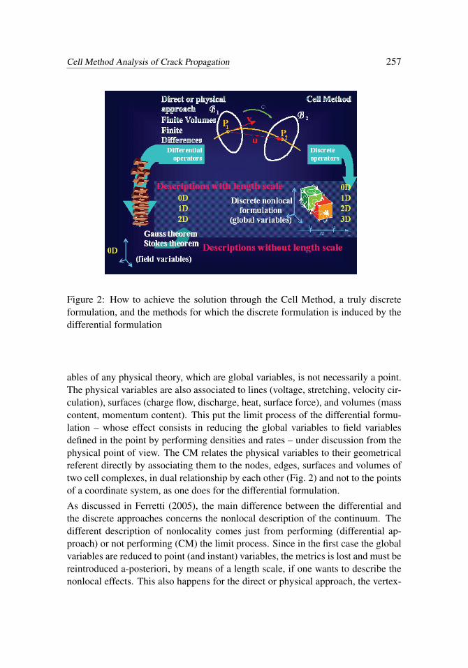
Figure 2: How to achieve the solution through the Cell Method, a truly discreteformulation, and the methods for which the discrete formulation is induced by thedifferential formulation

ables of any physical theory, which are global variables, is not necessarily a point.The physical variables are also associated to lines (voltage, stretching, velocity cir-culation), surfaces (charge flow, discharge, heat, surface force), and volumes (masscontent, momentum content). This put the limit process of the differential formu-lation – whose effect consists in reducing the global variables to field variablesdefined in the point by performing densities and rates – under discussion from thephysical point of view. The CM relates the physical variables to their geometricalreferent directly by associating them to the nodes, edges, surfaces and volumes oftwo cell complexes, in dual relationship by each other (Fig. 2) and not to the pointsof a coordinate system, as one does for the differential formulation.

As discussed in Ferretti (2005), the main difference between the differential andthe discrete approaches concerns the nonlocal description of the continuum. Thedifferent description of nonlocality comes just from performing (differential ap-proach) or not performing (CM) the limit process. Since in the first case the globalvariables are reduced to point (and instant) variables, the metrics is lost and must bereintroduced a-posteriori, by means of a length scale, if one wants to describe thenonlocal effects. This also happens for the direct or physical approach, the vertex-


based scheme of the Finite Volume Method, and the Finite Differences Method.Both could be considered very similar to the CM while they start from point-wiseconservation equations and derive the discrete formulation by the differential for-mulation (Fig. 2). With the CM, oppositely, we do not need to recover the lengthscale since it is preserved by avoiding the limit process (Fig. 2). As a consequence,the CM allows for obtaining a nonlocal formulation by using local constitutivelaws.

Recently, Heshmatzadeh and Bridges (2007) have compared in detail CM and FEMin electrostatics, proving the equivalence of the coefficient matrices for a Voronoidual mesh and linear shape functions in the FEM, also showing that the use oflinear shape functions in FEM is equivalent to the use of a barycentric dual meshfor charge vectors.

The numerical code for crack trajectory analysis with the CM has been developedby the author [Ferretti (2003, 2008)]. In this study, the code has been extendedto provide results in the case of a concrete plate tensioned at infinity by a load ofintensity px = kp0 parallel to the x-axis and py = p0 parallel to the y-axis (Fig. 1).The plate has an initial straight crack of length 2l0 oriented at an angle α0 to thex-axis (β0 to the y-axis). The crack trajectory and the minimum load required topropagate the crack from the ends of the cut are provided for various values of kand α0.

3 Crack extension criterion

The minimum load required to propagate a crack (limiting load) can be deduced byusing a variety of criteria:

• maximal normal stress criterion;

• maximal strain criterion;

• minimum strain energy density fracture criterion;

• maximal strain energy release rate criterion;

• damage law criteria.

In the present paper, the crack extension condition is studied in the Mohr-Coulombplane. The limiting load is computed as the load satisfying the condition of tan-gency between the Mohr’s circle representing the stress field in the neighborhoodof the tip and the Leon limit surface (Fig. 3). With c being the cohesion, fc thecompressive strength, ftb the tensile strength, τn and σn, respectively, the shear


and normal stress on the attitude of external normal n, the Leon criterion in theMohr-Coulomb plane is expressed as:

τ2n =

cfc

(ftbfc

+σn

). (3)

σn

τn

Mohr's pole

Mohr's circle

crack propagation direction

Leon limitsurface

Figure 3: Leon limit surface

Delaunay Voronoi

•

••

•

• •

•

••

crack

hexagonal element

Figure 4: Hexagonal element for stressanalysis at the crack tip

The Mohr’s circle for the tip neighborhood is identified by means of the physicalsignificance associated with the CM domain discretization: the CM divides the do-main by means of two cell complexes, in such a way that each cell of the first cellcomplex, which is a simplicial complex, contains one, and one only, node of thesecond cell complex (in this study, a Delaunay/Voronoi mesh generator is used togenerate the two meshes in two-dimensional domains). The primal mesh (the De-launay mesh) is obtained by subdividing the domain into triangles, so that for eachtriangle of the triangulation the circumcircle of that triangle is empty of all othersites (Fig. 4). The dual mesh (the Voronoi mesh) is formed by the polygons whosevertexes are at the circumcenters of the primal mesh (Fig. 4). For each Voronoisite, every point in the region around that site is closer to that site than to any ofthe other Voronoi sites. Now, the conservation law is enforced on the dual poly-gon of every primal vertex [Ferretti (2003)] and the stresses are computed on thenodes of the dual mesh. Thus, not only the displacements, like in the FEM, but alsothe stresses are primary outputs of a CM code and it is no longer necessary to usepoint matching techniques to determine stresses and SIFs. The crack propagationdirection is then derived in the Mohr/Coulomb plane directly as the line joining theMohr’s pole to the point in which the circle of Mohr is tangent to the limit surface.In effect, both lines joining one of the two tangent points at the limiting stage to


the Mohr’s pole identify propagation directions. For the plate in Fig. 1, due to thebiaxial state of tensile stress at the ends of the cut, the Mohr’s circle of the atti-tudes making bundle around the z-axis is fully contained in the positive half-planeof the normal stress. It follows that the Mohr’s circle at the limiting stage is tangentto the limit surface of Leon in just one point, the vertex of the parabola of Leon(Fig. 3). Consequently, just one propagation direction activates at each stage ofthe propagation process.

In order to identify the Mohr’s circle for the tip neighborhood, a hexagonal elementhas been inserted at the tip ([Ferretti (2003)], Fig. 4). When the mesh generator isactivated, the hexagonal element is divided into equilateral Delaunay triangles anda quasi-regular tip Voronoi cell is generated (the cell filled in gray in Fig. 4). Thisallow us to establish a correspondence between the tip stress field and the attitudescorresponding to the sites of the tip Voronoi cell. It has been shown [Ferretti (2003)]that the tension points correctly describe the Mohr’s circle in the Mohr-Coulombplane, for rotation of the hexagonal element around the tip.

The used crack propagation technique is the intra-element technique with nodalrelaxation and subsequent re-meshing. Extension of this technique to the activationof two propagation directions is provided in Ferretti (2008) even for the case inwhich crack bifurcation occurs during propagation.

4 Constitutive Assumption

The concrete constitutive law adopted in this study is monotonic non-decreasing,in accordance with the identification procedure for concrete in mono-axial loadprovided in Ferretti (2005) (Fig. 5). It was shown [Ferretti (2004b, 2005)] howthis constitutive law turned out to be size insensitive for mono-axial compressiveload. This result has made it possible to formulate a new concrete law in mono-axial loading, the effective law, which can be considered more representative of thematerial physical properties than the softening laws are. Now, the effective law istested for applications in bi-axial tensile load. The tensile branch has been hereidentified starting from the compressive one, in the assumption that a homotheticrelationship exists between the two branches (Fig. 5). A ratio between tensile andcompressive strength of 1/12, 1/8, 1/6, 1/4, 1/3 and 1/2 has been considered. Thebest accordance between analytical and experimental results has been obtained forthe ratio equal to 1/8.

5 Parametric analysis of the limiting load

Numerical results concerning the limiting load for the concrete plate loaded asshown in Fig. 1 are here presented. For symbols and conventions, refer to Fig. 1.


ε

σ

Figure 5: Adopted constitutive law for concrete in mono-axial load

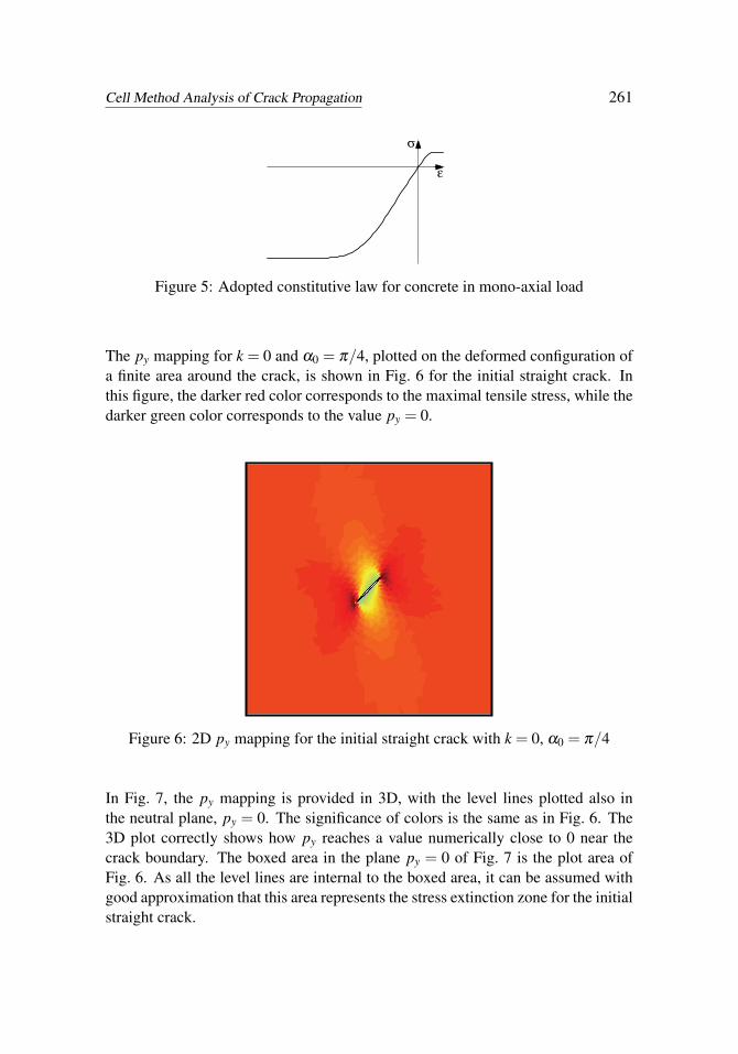
The py mapping for k = 0 and α0 = π/4, plotted on the deformed configuration ofa finite area around the crack, is shown in Fig. 6 for the initial straight crack. Inthis figure, the darker red color corresponds to the maximal tensile stress, while thedarker green color corresponds to the value py = 0.

Figure 6: 2D py mapping for the initial straight crack with k = 0, α0 = π/4

In Fig. 7, the py mapping is provided in 3D, with the level lines plotted also inthe neutral plane, py = 0. The significance of colors is the same as in Fig. 6. The3D plot correctly shows how py reaches a value numerically close to 0 near thecrack boundary. The boxed area in the plane py = 0 of Fig. 7 is the plot area ofFig. 6. As all the level lines are internal to the boxed area, it can be assumed withgood approximation that this area represents the stress extinction zone for the initialstraight crack.


Neutral plane

Figure 7: 3D py mapping and lines of equal py for the initial straight crack withk = 0, α0 = π/4

The normalized limiting load in the direction of the y-axis for a prefixed value ofthe load ratio k:

pylim (α0,k)|k=const =pylim (α0,k)|k=const

pymax

, (4)

with:

pymax = maxα0,k

pylim (α0,k) , (5)

is plotted in Fig. 8 in function of the angle α0 (or, which is the same, in functionof β0 = π/2−α0) for the factor k equal to 0, 1/4, 1/2, 3/4 and 1. The figureexhibits a pylim limiting load increasing with α0 for each constant value of k in thefield 0≤ k < 1, stating that the value α0 = 0 gives the critical crack orientation forall the biaxial load conditions, the x-component being lower than the y-component.The constant behavior of the relationship obtained for k = 1 is in good agreementwith the homogeneous state of stress represented by this load condition. In thiscase, all the crack orientations to the x-axis return the same limiting load.

The limiting load pylim for a given load ratio k = k and a given crack inclinationα0 = α0 is the same as the limiting load pxlim for the reciprocal load ratio k = 1/k


30%

40%

50%

60%

70%

80%

90%

100%

0 10 20 30 40 50 60 70 80 90Crack inclination to the y-axis, β0

Nor

mal

ised

lim

iting

load

py/p

ymax

0102030405060708090Crack inclination to the x-axis, α0

k=0

K=1/4

K=1/2

K=1

K=3/4

[deg]

[deg]

limm

axy

yp

p

Figure 8: Normalized limiting load pylim in function of the crack inclinations α0and β0 for 0≤ k ≤ 1

and the complementary crack inclination β0 = α0. By defining the ideal limitingload pidlim as:

pidlim =√

p2xlim

+ p2ylim

= p0lim

√k2 +1, (6)

it follows that pidlim assumes the same values for load conditions and crack incli-nations which both are symmetric with respect to the bisector of the first quadrant,y = x, with x and y the axes in Fig. 1.

The line y = x superimposes to the crack when the crack is oriented at the angleα0 = π/4 (or, which is the same, at the angle β0 = π/4). Thus, in the plane α0/pidlim

(or β0/pidlim) the curves of the ideal limiting load for the given value k of k andits reciprocal value k = 1/k are symmetric with respect to the line α0 = π/4 (orβ0 = π/4).

In Fig. 9, the curves of the normalized ideal limiting load for a prefixed value ofthe load ratio k:

pidlim (α0,k)|k=const =pidlim (α0,k)|k=const

pidmax

, (7)

with:

pidmax = maxα0,k

pidlim (α0,k) , (8)


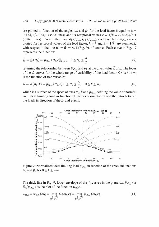
are plotted in function of the angles α0 and β0 for the load factor k equal to k =0,1/4,1/2,3/4,1 (solid lines) and its reciprocal values k = 1/k = ∞,4,2,4/3,1(dotted lines). Even in the plane α0/pidlim (β0/ pidlim), each couple of pidlim curvesplotted for reciprocal values of the load factor, k = k and k = 1/k, are symmetricwith respect to the line α0 = β0 = π/4 (Fig. 9), of course. Each curve in Fig. 9represents the function:

fk = fk (α0) = pidlim (α0,k)|k=k , 0≤ α0 ≤π

2(9)

returning the relationship between pidlim and α0 at the given value k of k. The locusof the fk curves for the whole range of variability of the load factor, 0 ≤ k ≤ +∞,is the function of two variables:

Ω = Ω(α0,k) = pidlim (α0,k) 0≤ α0 ≤π

2, 0≤ k ≤ ∞, (10)

which is a surface of the space of axes α0, k and pidlim defining the value of normal-ized ideal limiting load in function of the crack orientation and the ratio betweenthe loads in direction of the x- and y-axis.

40%

50%

60%

70%

80%

90%

100%

0 10 20 30 40 50 60 70 80 90Crack inclination to the y-axis, β0

Nor

mal

ised

idea

l lim

iting

load

pid

/pid

max

0 10 20 30 40 50 60 70 80 90 100Crack inclination to the x-axis, α0

k=0

k=1/4

k=1/2

k=1

k=3/4

k=h

k=4

k=2

k=4/3

0102030405060708090Crack inclination to the x-axis, α0 [deg]

0 0 45α β= = °limm

axid

idp

p

100%

Figure 9: Normalized ideal limiting load pidlim in function of the crack inclinationsα0 and β0 for 0≤ k ≤+∞

The thick line in Fig. 9, lower envelope of the fk curves in the plane α0/ pidlim (orβ0/ pidlim), is the plot of the function wα0k:

wα0k = wα0k (α0) = minα0=α00≤k≤∞

Ω(α0,k) = minα0=α00≤k≤∞



with:

0≤ α0 ≤π

2. (12)

Each point of the function (11) is obtained for different values of the load factork and, thus, belongs to different fk curves. Consequently, wα0k is the projectionon the plane α0/pidlim (or β0/ pidlim) of a 3D function of the space of axes α0, kand pidlim , named ωα0 , where α0 and k are not independent variables since theyare bonded by the condition (11) of minimum load. Said kcr

lim = kcrlim (α0) the load

factor providing the minimum value of normalized ideal limiting load pidlim for eachassigned α0 = α0:

kcrlim (α0) = k : pidlim |α0=α0

k=kcrlim

= minα0=α00≤k≤∞

pidlim (α0,k) , 0≤ α0 ≤π

2(13)

the function ωα0 returning the minimum pidlim for a given α0 = α0 and 0≤ k≤+∞

can be written as:

ωα0 = ωα0 (α0,kcrlim) = min

α0=α00≤k≤∞

Ω(α0,k) = minα0=α00≤k≤∞


with:

0≤ α0 ≤π

2. (15)

The function (13), where kcrlim is the ratio between pcr

x and pcry at the limit state, is

provided by the projection of ωα0 on the plane α0/k, said wα0 p (Fig. 10):

wα0 p = wα0 p (α0) = kcrlim (α0) . (16)

kcrlim can be also expressed as the solution of the following differential problem:

kcrlim = kcr

lim (α0) = k :∂ pidlim (α0,k)

∂k

∣∣∣∣α0=α0k=kcr

lim

= 0,∂ 2 pidlim (α0,k)

∂k2

∣∣∣∣α0=α0k=kcr

lim

> 0 (17)

In the aim to plot the 3D surface of the normalized ideal limiting load given byEq. (10) for the whole range of variability of the load factor, 0 ≤ k ≤ +∞, thesecond independent variable of Ω, k, has been substituted by the variable ψ definedas follows:

ψ = ψ (k) = 1− e−k, 0≤ k ≤+∞. (18)


0

1

2

3

4

5

6

7

8

0 10 20 30 40 50 60 70 80 90

Crack inclination to the y-axis, β0 [deg]

Crit

ical

load

fact

or k

lim

0102030405060708090

Crack inclination to the x-axis, α0 [deg]

Figure 10: Load factor kcrlim providing the minimum value of pidlim for each assigned

α0 = α0

With the change of variable (18), the surface of the normalized ideal limiting loadis given by the function:

Ω = Ω(α0,ψ) = pidlim (α0,ψ) , 0≤ α0 ≤π

2, 0≤ ψ ≤ 1, (19)

which substitutes Eq. (10). The Eq. (19) gives a finite 3D representation of pid ,in function of α0 (or β0) and ψ , since the ranges of variability of its independentvariables are finite ranges (Eq. (19)).

Some plots of Ω obtained for different axes orientation are given in Fig. 11. Inparticular, Fig. 11.a is the 3D equivalent representation of Fig. 9. Each line inFig. 11.a represents the function:

fψ = fψ (α0) = pidlim (α0,ψ)|ψ=ψ

, 0≤ α0 ≤π

2, (20)

returning the relationship between pidlim and α0 at the given value ψ of ψ . Since thedifference between the two surfaces Ω and Ω stands in the change of the variableplotted along the axis which is orthogonal both to the planes of Fig. 9 and Fig. 11.a(Eq. (18)), it follows that the plot of the function fk is equal to that of the functionfψ :

fk (α0)|k=k = fψ (α0)∣∣ψ=ψ=1−e−k , 0≤ α0 ≤

π

2. (21)


limm

axid

idp

p

( )ˆ 0fψ ψ = ( )ˆ 1fψ ψ =

Ω

0 0ˆˆ , wα ψ αω

limm

axid

idp

p

limm

axid

idp

p

0.63

( )0 0

ˆ 90fα α =

( )0 0

ˆ 0fα α =

Ω

ˆψω

ˆ pwψ

limm

axid

idp

p

( )ˆ 0fψ ψ =

( )ˆ 1fψ ψ =

Ω

0ˆ pwα

0ˆαω

limm

axid

idp

p

0.63

( )0 0

ˆ 90fα α = ( )

0 0ˆ 0fα α =

0ˆˆ , wψα ψω

Ω

limm

axid

idp

p

a) b)

c) d)

e) f)

Figure 11: Some examples of finite 3D representation of pidlim , in function of β0and ψ


The lower envelope of the fψ curves in the plane α0/pidlim (or β0/pidlim) is thefunction wα0ψ (Fig. 11.a):

wα0ψ = wα0ψ (α0) = minα0=α00≤ψ≤1

Ω(α0,ψ) = minα0=α00≤ψ≤1

pidlim (α0,ψ) , (22)

with:

0≤ α0 ≤π

2. (23)

Once more, from Eq. (18) it follows that:

wα0k (α0)|k=k = wα0ψ (α0)∣∣ψ=ψ=1−e−k , 0≤ α0 ≤

π

2. (24)

0

0.1

0.2

0.3

0.4

0.5

0.6

0.7

0.8

0.9

1

0 10 20 30 40 50 60 70 80 90

Crack inclination to the y-axis, β0 [deg]

Crit

ical

load

fact

or ψ

lim

0.00

0.10

0.20

0.30

0.40

0.50

0.60

0.70

0.80

0.90

1.00

0102030405060708090

Crack inclination to the x-axis, α0 [deg]

Crit

ical

load

fact

or k

lim

∞

2.30

1.61

1.20

0.92

0.69

0.51

0.36

0.22

0.11

0.00

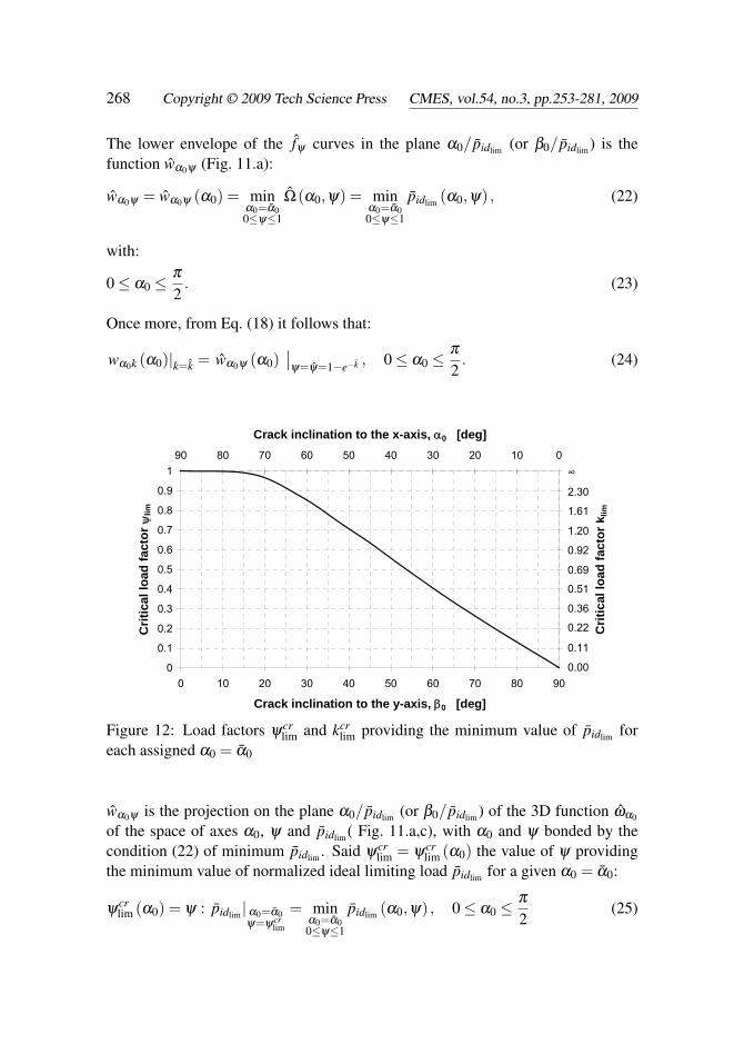
Figure 12: Load factors ψcrlim and kcr

lim providing the minimum value of pidlim foreach assigned α0 = α0

wα0ψ is the projection on the plane α0/ pidlim (or β0/pidlim) of the 3D function ωα0

of the space of axes α0, ψ and pidlim( Fig. 11.a,c), with α0 and ψ bonded by thecondition (22) of minimum pidlim . Said ψcr

lim = ψcrlim (α0) the value of ψ providing

the minimum value of normalized ideal limiting load pidlim for a given α0 = α0:

ψcrlim (α0) = ψ : pidlim | α0=α0

ψ=ψcrlim

= minα0=α00≤ψ≤1

pidlim (α0,ψ) , 0≤ α0 ≤π

2(25)


the function ωα0 can be written as:

ωα0 = ωα0 (α0,ψcrlim) = min

α0=α00≤ψ≤1

Ω(α0,ψ) = minα0=α00≤ψ≤1


with:

0≤ α0 ≤π

2. (27)

The projection of the function ωα0 on the plane α0/ψ , named wα0 p in Fig. 11.c,returns the relationship between ψcr

lim and α0 (Fig. 12):

wα0 p = wα0 p (α0) = ψcrlim (α0) . (28)

In Fig. 12 also the axis of the load factor kcrlim is plotted in order to make it possible

to evaluate the effect of the change of variable (18) on the law of the minimumpidlim , by comparing the two functions given by Eqs. 16, plotted in Fig. 10, and 28,plotted in Fig. 12.

The function ψcrlim can be also expressed as the solution of the following differential

problem:

ψcrlim = ψ

crlim (α0) = ψ :

∂ pidlim (α0,ψ)∂ψ

∣∣∣∣ α0=α0ψ=ψcr

lim

= 0,∂ 2 pidlim (α0,ψ)

∂ψ2

∣∣∣∣ α0=α0ψ=ψcr

lim

> 0

(29)

The Fig. 11.f is obtained by a 90˚ rotation of the Ω surface around the pid-axis.This last plot represents the locus of the functions:

fα0 = fα0 (ψ) = pidlim (α0,ψ)|α0=α0

, 0≤ ψ ≤ 1 (30)

returning the relationship between pidlim and ψ for each assigned value α0 of α0.The functions fα0 are the meridians of the surface in Fig. 11.f.

The lower envelope of the fα0 functions gives the function (Fig. 11.f):

wψα0 = wψα0 (ψ) = min0≤α0≤ π

2ψ=ψ

Ω(α0,ψ) = min0≤α0≤ π

2ψ=ψ


with:

0≤ ψ ≤ 1. (32)


wψα0 is the projection on the plane ψ/pidlim of the 3D function ωψ plotted in Figs.11.d,f:

ωψ = ωψ (αcr0 ,ψ) = min

0≤α0≤ π

2ψ=ψ

Ω(α0,ψ) = min0≤α0≤ π

2ψ=ψ


where:

αcr0 = α

cr0 (ψ) = α0 : pidlim |α0=αcr

0ψ=ψ

= min0≤α0≤ π

2ψ=ψ

pidlim (α0,ψ) , 0≤ ψ ≤ 1 (34)

is the crack inclination minimizing the normalized ideal limiting load pidlim foreach assigned load factor ψ = ψ . That is to say, as for ωα0 and ωα0 also the twovariables of ωψ are bonded by a condition of minimum load. αcr

0 is the solution ofthe following differential problem:

αcr0 = α

cr0 (ψ) = α0 :

∂ pidlim (α0,ψ)∂α0

∣∣∣∣α0=αcr0

ψ=ψ

= 0,∂ 2 pidlim (α0,ψ)

∂α20

∣∣∣∣α0=αcr

0ψ=ψ

> 0

(35)

As can be seen in Fig. 11.f, all the fα0 functions intersect in one point, of firstcoordinate:

ψ = 1− 1e∼= 0.63. (36)

From Eqs. (36) and (18) it follows that the intersection point of all the fα0 functionsis found for the value of the load ratio:

k =− log(1−ψ) = 1. (37)

Since the fα0 functions do not have any other point in common, the α0 = αcr0 min-

imizing pidlim at a given ψ turns out to be equal to:

αcr0 =

0 0≤ ψ < 1− 1

e , 0≤ k < 1[0, π

2

]ψ = 1− 1

e , k = 1π

2 1− 1e < ψ ≤ 1, 1 < k ≤+∞

(38)

which means that, as already observed in Fig. 8:

αcr0 =

0 px < py

[0,π/2] px = py

π/2 px > py

(39)


Eq. (38), gives the values of the function wψ p, projection of ωψ on the plane ψ/α0(Fig. 11.d):

wψ p = wψ p (ψ) = αcr0 (ψ) . (40)

The two functions ωα0 and ωψ have just one point in common (Fig. 11.c,d), thepoint for which both functions are stationary:

α0 = β0 =π

4, ψ = 1− 1

e. (41)

Actually, in a point in which both functions are stationary, looking for the minimumpidlim at constant α0 is equal to looking for the minimum pidlim at constant ψ:

minα0= π

40≤ψ≤1

pidlim (α0,ψ) = min0≤α0≤ π

2ψ=1− 1

e

pidlim (α0,ψ) = min0≤α0≤ π

2k=1

pidlim (α0,k) . (42)

6 Parametric analysis of the propagation path

In Fig. 13 and Fig. 14, the 2D and 3D py analysis for k = 0 and α0 = π/4 isshown for a generic crack propagation step. The lighter colors of Figs. 13 and 14with respect to those of Figs. 6 and 7 are representative of the progressive platedownloading corresponding to the crack propagation. For the same reason, thevalues in the third axis of Fig. 14 are smaller than those of Fig. 7. Moreover, inFig. 13 it can be observed how a mono-axial compressive state of stress of smallentity (cyan color) arises in the plate, due to the geometrical effect of the non-straight crack deformation in Mode I.

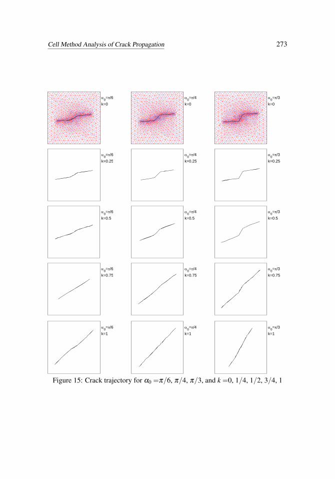
The crack trajectory is plotted in Fig. 15 for the value of the angle α0 equal toπ/6, π/4 and π/3, and for the factor k equal to 0, 1/4, 1/2, 3/4 and 1. In thisfigure, also the two meshes of Delaunay-Voronoi were plotted for k = 0, in orderto show how the adaptive mesh generator recreates the meshes for a generic crackpropagation step (Delaunay mesh in red and Voronoi mesh in blue, as indicatedin Fig. 4). Fig. 15 shows that the crack trajectory tends to approach an asymptoteperpendicular to the external tensile load for all the three cases with k = 0. Theasymptotic behavior is also evident for k > 0, but the asymptote is now oriented atan angle γ to the x-axis which depends on k:

γ = f (k) . (43)

The angle γ does not depend on the inclination α0 of the initial straight crack, sincethe crack tends to propagate perpendicularly to the tensile principal direction of the


Figure 13: 2D py mapping for a generic propagation step with k = 0, α0 = π/4

Figure 14: 3D py mapping and lines of equal py for a generic propagation step withk = 0, α0 = π/4

uncracked plate. For k = 1, the angle γ assumes the value π/4, in good accordancewith the homogeneous state of stress represented by this load condition:

γ|k=1 =π

4. (44)

The plot of the function γ = f (k) is provided in Fig. 16 for the range of values


α0=π/6k=0 k=0

α0=π/4k=0α0=π/3

α0=π/3k=0.75

α0=π/6k=0.75

α0=π/3k=0.5

α0=π/4k=0.5

α0=π/4k=0.25 k=0.25

α0=π/3α0=π/6k=0.25

α0=π/6k=0.5

α0=π/4k=0.75

k=1α0=π/6 α0=π/4

k=1α0=π/3k=1

Figure 15: Crack trajectory for α0 =π/6, π/4, π/3, and k =0, 1/4, 1/2, 3/4, 1


0≤ k≤ 1. The plot of γ for the complete range of values 0≤ k≤+∞ (Fig. 17) canbe provided by means of the change of variable given by Eq. (18).

0

0.025

0.05

0.075

0.1

0.125

0.15

0.175

0.2

0.225

0.25

0 0.1 0.2 0.3 0.4 0.5 0.6 0.7 0.8 0.9 1

Ratio between the load parallel to the x - and to the y -axis, k

Asy

mpt

otic

incl

inat

ion

to th

e x

-axi

s, γ

(rad

)

Figure 16: Relationship between the angle γ and the load ratio k

0

0.05

0.1

0.15

0.2

0.25

0.3

0.35

0.4

0.45

0.5

0 0.1 0.2 0.3 0.4 0.5 0.6 0.7 0.8 0.9 1

ψ =1-e-k

Asy

mpt

otic

incl

inat

ion

to th

e x

-axi

s, γ

(r

ad)

k =1/4

k =1/2

k =1

k =2k =4

k =+h

k =0

k =3/4

k =4/3

Figure 17: Relationship between the angle γ and the variable ψ

If the behavior of the function γ = f (k) for 0 ≤ k ≤ 1 is known, the behavior ofγ = f (k) for 1 < k ≤ +∞ is also known. Actually, the asymptotes of the cracktrajectory for a given k and its reciprocal value, 1/k, are symmetric with respect tothe bisector of the first quadrant in Fig. 1, y = x (Fig. 18). That is to say, the value


ϕ

ϕ

Crack trajectoryfor a given kCrack trajectoryfor a given k

Crack trajectoryfor 1/kCrack trajectoryfor 1/k

Figure 18: Crack trajectories for a given k and 1/k

assumed by γ for a given k is equal to the complementary angle of γ for 1/k:

γ

(1k

)=

π

2− γ (k) . (45)

Naming ϕ the clockwise positive angle in Fig. 18, with:

ϕ =π

4− γ, (46)

from Eqs. 45 and 46, it follows that:

ϕ

(1k

)=−ϕ (k) . (47)

7 Conclusions

A first study on tensioned concrete plates was presented, based on an innovativesize-insensitive constitutive law.

The numerical model adopted, based on the CM, allows analysis in the discrete.The crack propagation is then studied without using the stress intensity factors andwithout having to define a model to treat the zone ahead of the crack tip. This allowsone to employ the same numerical code for bodies of different dimensions, geome-tries and boundary conditions, and for materials of different constitutive laws. Asan example of the code versatility in front of the geometrical set-up, the interactionbetween two or more cracks oriented at any inclination and propagating in plateof finite/infinite dimensions can be easily investigated. As far as the versatility infront of the constitutive law is concerned, the numerical analysis can be indiffer-ently performed in the linear and non-linear field, with no adjunctive computationalburdens.


The stress intensity factors of the variational approach can be estimated a-posteriori,since the code allows us to evaluate the compliance decrement following from crackpropagation. A comparison between the variational and discrete formulation is thenpossible, and it will be investigated in future studies.

In this paper, it was shown how the numerical results for plates in bi-axial loadingare satisfactory with respect to the load and geometrical parameters.

The crack trajectory exhibits an asymptotic behavior which only depends on theratio between the load parallel to the x- and the y-axis, k, being insensitive to theinclination α0 of the initial straight crack. The crack always tends to propagate per-pendicularly to the tensile principal direction of the uncracked plate. The numeri-cal law of the asymptotic inclination, said γ = f (k), was provided for the completevariability range of k, k = [0,+∞].The plausibility of the founded crack trajectories in dependence on the parameterk indirectly gives a validation of the adopted constitutive law for bi-axial tensileloading.

It was also shown how the numerical crack trajectory for a solid of finite dimensionsis highly accurate.

Finally, it is remarkable how the analysis for finite solids is performed directly,without having to apply corrective factors to the solution on an infinite geometry inthe same load conditions.

Acknowledgement: This work was made possible by the Italian Ministry forUniversities and Scientific and Technological Research (MURST).

8 References

Abdelaziz, Y.; Abou-bekr, N.; Hamouine, A. (2007): Numerical Modeling of theCrack Tip Singularity. Int. J. Mater. Sci., vol. 2, pp. 65-72.

Alotto, R.P.; Codecasa, L.; Freschi, F.; Gruosso, G.; Moro, F.; Repetto, M.(2006): Finite Formulation for Quasi-Magnetostatics with Integral Boundary Con-ditions. 11th International IGTE Symposium Proceedings, September 18-20, Graz(Austria), CD form.

Alotto, R.P.; Gruosso, G.; Moro, F.; Repetto, M. (2008): A Boundary IntegralFormulation for Eddy Current Problems Based on the Cell Method. IEEE Trans.on Magnetics, vol. 44, pp. 770-773.

Alotto, R.P.; Perugia I. (2004): Matrix Properties of a Vector Potential Cell Methodfor Magnetostatics. IEEE Trans. on Magnetics, vol. 40, no. 2, pp. 1045-1048.

Alshoaibi, A.; Hadi, M.; Ariffin, A. (2007): Two-Dimensional Numerical Estima-


tion of Stress Intensity Factors and Crack Propagation in Linear Elastic Analysis.J. Struct. Durability Health Monit., vol. 3, pp. 15-28.

Anderson, T.L. (1991): Fracture Mechanics, Fundamentals and Applications, CRCPress.

Aour, B.; Rahmani, O.; Nait-Abdelaziz, B. (2007): A Coupled FEM/BEM Ap-proach and its Accuracy for Solving Crack Problems in Fracture Mechanics. Int. J.Solids Struct., vol. 44., pp. 2523- 2539.

Bettini, P.; Trevisan, F. (2003): Electrostatic Analysis for Plane Problems withFinite-formulation. IEEE Trans. on Magnetics, vol. 39, no. 3, pp. 1127-1130.

Bottauscio, O.; Manzin, A.; Canova, A.; Chiampi, M.; Guosso, G.; Repetto,M. (2004): Field and Circuit Approaches for Diffusion Phenomena in MagneticCores. IEEE Trans. on Magnetics, vol. 40, no. 2, pp. 1322-1325.

Bowie, O.L. (1956): Analysis of an Infinite Plate Containing Radial Cracks orig-inating at the Boundary of an Internal Circular Hole. J. Math. Phys., vol. 35, pp.60-71.

Broek. D. (1974): Elementary Engineering Fracture Mechanics, Nordhoff Interna-tional Publishing.

Bullo, M.; D’Ambrosio, V.; Dughiero, F.; Guarnieri, M. (2006): Coupled Elec-tric and Thermal Transient Conduction Problems with a Quadratic InterpolationCell Method Approach. IEEE Trans. on Magnetics, vol. 42, no. 4, pp. 1003-1006.

Bullo, M.; D’Ambrosio, V.; Dughiero, F.; Guarnieri, M. (2007): A 3D CellMethod Formulation for Coupled Electric and Thermal Problems. IEEE Trans. onMagnetics, vol. 43, no. 4, pp. 1197-1200.

Chang, R. (1981): Static Finite Element Stress Intensity Factors for annular Cracks.J. Nondestruct. Evaluat., vol. 2, pp. 119-124.

Codecasa, L.; Specogna, R.; Trevisan, F. (2008): Discrete Constitutive Equationsover Hexahedral Grids for Eddy-Current Problems. CMES: Computer Modeling inEngineering & Sciences, vol. 31, no. 3, pp. 129-144.

Cosmi, F. (2001): Numerical Solution of Plane Elasticity Problems with the CellMethod. CMES: Computer Modeling in Engineering & Sciences, vol. 2, no. 3, pp.365-372.

Cosmi, F. (2003): Numerical Modeling of Porous Materials Mechanical Behaviourwith the Cell Method. Proceedings of the Second MIT Conference on Computa-tional Fluid and Solid Mechanics, Massachusetts Institute of Technology, Cam-bridge (MA, U.S.A.), pp. 17-20.

Cosmi, F. (2005): Elastodynamics with the Cell Method. CMES: Computer Mod-eling in Engineering & Sciences, vol. 8, no. 3, pp. 191-200.


Cosmi, F. (2008): Dynamical Analysis of Mechanical Components: a DiscreteModel for Damping. CMES: Computer Modeling in Engineering & Sciences, vol.27, no. 3, pp. 187-195.

Cosmi, F.; Di Marino, F. (2001): Modelling of the Mechanical Behaviour ofPorous Materials: a New Approach. Acta of Bioengineering and Biomechanics,vol. 3, no. 2, pp. 55-66.

Cosmi, F.; Dreossi, D. (2007): The Application of the Cell Method for the ClinicalAssessment of Bone Fracture Risk. Acta of Bioengineering and Biomechanics,Wroclaw University of Technology, Wroclaw (Poland), vol. 9, No. 2, pp. 35-39.

Cosmi, F.; Steimberg, N.; Dreossi, D.; Mazzoleni, G. (2009): Structural Analysisof Rat Bone Explants in Vitro in Simulated Microgravity Conditions. J. Mech.Behav. Biomed. Mater., vol. 2, no. 2, pp. 164-172.

De Araújo, T.; Bittencourt, T.; Roehl, D.; Martha, L. (2000): Numerical Esti-mation of Fracture Parameters in Elastic and Elastic-Plastic Analysis. Proceedingsof the European Congress on Computational Methods in Applied Sciences and En-gineering, September 11-14, Barcelona (Spain), pp. 1-18.

Dugdale, D.S. (1960): Yielding of Steel Sheets Containing Slits. J. Mech. Phys.Solids, vol. 8, no. 2, pp. 100-104.

Erdogan, F.; Sih, G.C. (1963): On the Extension of Plates under Plane Loadingand Transverse Shear. J. bas. Engng., vol. 85, pp. 519-527.

Ferretti, E. (2003): Crack Propagation Modeling by Remeshing using the CellMethod (CM). CMES: Computer Modeling in Engineering & Sciences, vol. 4, no.1, pp. 51-72.

Ferretti, E. (2004a): A Cell Method (CM) Code for Modeling the Pullout TestStep-wise. CMES: Computer Modeling in Engineering & Sciences, vol. 6, no. 5,pp. 453-476.

Ferretti, E. (2004b): Experimental Procedure for Verifying Strain-Softening inConcrete. Int. J. Fract. (Letters section), vol. 126, no. 2, pp. L27-L34.

Ferretti, E. (2004c): Crack-Path Analysis for Brittle and Non-brittle Cracks: aCell Method Approach. CMES: Computer Modeling in Engineering & Sciences,vol. 6, no. 3, pp. 227-244.

Ferretti, E. (2005): A Local Strictly Nondecreasing Material Law for ModelingSoftening and Size-Effect: a Discrete Approach. CMES: Computer Modeling inEngineering & Sciences, vol. 9, no. 1, pp. 19-48.

Ferretti, E.; Casadio, E.; Di Leo, A. (2008): Masonry Walls under Shear Test: aCM Modeling. CMES: Computer Modeling in Engineering & Sciences, vol. 30,no. 3, pp. 163-190.


Ferretti, E.; Di Leo, A. (2003): Modelling of Compressive Tests on FRP WrappedConcrete Cylinders through a Novel Triaxial Concrete Constitutive Law. SITA, vol.5, pp. 20-43.

Giuffrida, C.; Gruosso, G.; and Repetto, M. (2006): Finite Formulation of Non-linear Magnetostatics with Integral Boundary Conditions. IEEE Trans. on Magnet-ics, vol. 42, no. 5, pp. 1503-1511.

Griffith, A.A. (1920): The Phenomena of Rupture and Flow in Solids. Philos.Trans. Roy. Soc. London. Ser. A, vol. 221, pp. 163-198.

Gustavo, V.G.; Jaime, P.; Manuel, E. (2000): KI Evaluation by the DisplacementExtrapolation Technique. Eng. Fract. Mech., vol. 66, pp. 243-255.

Heckel, K. (1983): Einführung in die technische Anwendung der Bruchmechanik.Carl Hanser Verlag, München.

Hellen, T.K. (1975): On the Method of Virtual Crack Extensions. Int. J. Numer.Methods Eng., vol. 9, no. 1, pp. 187-207.

Heshmatzadeh, M.; Bridges, G.E. (2007): A Geometrical Comparison betweenCell Method and Finite Element Method in Electrostatics. CMES: Computer Mod-eling in Engineering & Sciences, vol. 18, no. 1, pp. 45-58.

Hussain, M.A.; Pu, S.L.; Underwood, J.H. (1974): Strain Energy Release Ratefor a Crack Under Combined Mode I and Mode II. Fracture Analysis ASTM STP,vol. 560, pp. 2-28.

Hutchinson, J.W. (1968): Singular Behaviour at the End of a Tensile Crack in aHardening Material. J. Mech. Phys. Solids, vol. 16, pp. 13-31.

Inglis, C.E. (1913): Stresses in a Plate due to the Presence of Cracks and SharpCorners. Proc. Institute Naval Architects.

Irwin, G.R. (1957): Analysis of Stresses and Strains Near the Ends of a CrackTraversing a Plate. J. Appl. Mech., vol. 24, no. 3, pp. 361-364.

Irwin, G.R. (1958): Fracture. In Flügge, S. (Ed.), Handbuch der Physik, vol. 6,Spinger, Berlin.

Koenke, C.; Harte, R.; Krätzing, W.B.; Rosenstein, O. (1998): On adaptiveRemeshing Techniques for Crack Simulation Problems. Eng. Computation, vol.15, no. 1, pp. 74-88.

Kutuka, M.A.; Atmacab, N.; Guzelbey, I.H. (2007): Explicit Formulation of SIFUsing Neural Networks for Opening Mode of Fracture. Int. J. Eng. Struct., vol.29, pp. 2080-2086.

Laurencin, J.; Delette, G.; Dupeux, M. (2007): An Estimation of Ceramic Frac-ture at Singularities by a Statistical Approach. J. Eur. Ceramic Soc., vol. 28, pp.


1-13.

Lenov, M.Y.; Panasyuk, V.V. (1959): Development of Minute Cracks in Solids.Prikl. Meckhanika, vol. 5, no. 4, pp. 391-401.

Marrone, M. (2004): Properties of Constitutive Matrices for Electrostatic andMagnetostatic Problems. IEEE Trans. on Magnetics, vol. 40, no. 3, pp. 1516-1520.

Marrone, M.; Mitra, R. (2004): A Theoretical Study of the Stability Criteria forGeneralized FDTD Algorithms for Multiscale Analysis. IEEE Trans. on Antennasand Propagation, vol. 52, no. 8.

Marrone, Grassi, P.; M.; Mitra, R. (2004): A New Technique Based on theCell Method for Calculation the Propagation Constant of Inhomogeneous FilledWaveguide. IEEE Trans. on Antennas and Propagation.

McClintock, F. (1958): Ductile Fracture Instability in Shear. J. Appl. Mech., vol.25, pp. 582-588.

Murakami, Y. (1978): A Method of Stress Intensity Factor Calculation for theCrack emanating from an arbitrarily shaped Hole or the Crack in the Vicinity of anarbitrarily shaped Hole. Trans. Jap. Soc. Mech. Eng., vol. 44, pp. 423-432.

Nappi, A.; Tin-Loi, F. (2001): A Numerical Model for Masonry Implemented inthe Framework of a Discrete Formulation. Struct. Eng. Mech., vol. 11, no. 2, pp.171-184.

Newman, J. (1971): An Improved Method of Collocation for the Stress Analysisof Cracked Plates with various shaped Boundaries. NASA TN., vol. 6376, pp.1-45.

Novozhilov, V.V. (1969): On the Foundations of the Theory of Equilibrium Cracksin Elastic Bodies. Prikl. Matem. i Mekhan., vol. 33, no. 5, pp. 797-812.

Owen, D. (1973): Stress Intensity Factors for Cracks in a Plate containing a Holeand in a spinning Disc. Int. J. Fract., vol. 4, pp. 471-476.

Paris, P.C.; Sih, G. (1965): Fracture Toughness Testing and its Applications. InASTM Special Technical Publication, no. 381, Philadelphia, pp. 30-81.

Patron, V.Z.; Morozov, E.M. (1978): Elastic-Plastic Fracture Mechanics. MIRPublishers.

Rice, J.R.; Rosengren, G.F. (1968): Plane Stain Deformation near a Crack Tip ina Power-Law Hardening Material. J. Mech. Phys. Solids, vol. 16, pp. 1-12.

Rolfe, S.T.; Barsom, J.M. (1987): Fracture and Fatigue Control in Structures,Applications of Fracture Mechanics, Prentice-Hall, Englewood Cliffs, NJ.

Shahani, A.; Tabatabaei, S. (2008): Computation of mixed Mode Stress Intensity


Factors in a Four-Point Bend Specimen. Applied Meth. Model., vol. 32, pp. 1281-1288.

Sih, G.C. (1974): Strain Energy Density Factor Applied to Mixed Mode CrackProblems. Int. J. Fract., vol. 10, pp. 321-350.

Sneddon, I.N. (1946): The Distribution of Stress in the Neighborhood of a Crackin an Elastic Solid. Proc. Roy. Soc. London, vol. A-187, pp. 229-260.

Souiyah, M.; Muchtar, A.; Alshoaibi, A.; Ariffin. A.K. (2009): Finite ElementAnalysis of the Crack Propagation for Solid Mechanics. Am. J. Applied Sci., vol.6, no. 7. pp. 1396-1402.

Specogna, R.; Trevisan, F. (2005): Discrete Constitutive Equations in A-χ Geo-metric Eddy-Current Formulation. IEEE Trans. on Magnetics, vol. 41, no. 4.

Stanislav, S.; Zdenek, K. (2008): Two Parameter Fracture Mechanics: FatigueCrack Behavior under Mixed Mode Conditions. Eng. Fract. Mech., vol. 75, pp.857-865.

Straface, S.; Troisi, S.; Gagliardi, V. (2006): Application of the Cell Method tothe Simulation of Unsaturated Flow. CMC: Computers, Materials and Continua,vol. 3, no. 3, pp. 155-166.

Taddei, F.; Pani, M.; Zovatto, L.; Tonti, E.; Viceconti, M. (2008): A New Mesh-less Approach for Subject-Specific Strain Prediction in Long Bones: Evaluation ofAccuracy. Clin. Biomech., vol. 23, no. 9, pp. 1192-1199.

Tonti, E. (2001a): A Direct Discrete Formulation of Field Laws: the Cell Method.CMES: Computer Modeling in Engineering & Sciences, vol. 2, no. 2, pp. 237-258.

Tonti, E. (2001b): A Direct Discrete Formulation for the Wave Equation. J. Com-put. Acoust., 9(4): 1355-1382.

Tonti, E.; Zarantonello, F. (2009): Algebraic Formulation of Elastostatics: theCell Method. CMES: Computer Modeling in Engineering & Sciences, vol. 39, no.3, pp. 201-236.

Trevisan, F.; Kettunen, L. (2004): Geometric Interpretation of Discrete Approachesto Solving Magnetostatics. IEEE Trans. on Magnetics, vol. 40, no. 2.

Wells, A.A. (1961): Unstable Crack Propagation in Metals: Cleavage and FastFracture. Proc. Crack Propagation Symposium, vol. 1, College of Aeronautics andthe Royal Aeronautical Society, Cranfield (England), pp. 210-230.

Yan, X. (2006): Cracks emanating from Circular Hole or Square Hole in Rectan-gular Plate in Tension. Eng. Fract. Mech., vol. 73, pp. 1743-1754.

CMES is Indexed & Abstracted inApplied Mechanics Reviews; Cambridge Scientific Abstracts (Aerospace and High

Technology; Materials Sciences & Engineering; and Computer & InformationSystems Abstracts Database); CompuMath Citation Index; Current Contents:

Engineering, Computing & Technology; Engineering Index (Compendex); INSPECDatabases; Mathematical Reviews; MathSci Net; Mechanics; Science Alert; Science

Citation Index; Science Navigator; Zentralblatt fur Mathematik.

CMES: Computer Modeling in Engineering & Sciences

ISSN : 1526-1492 (Print); 1526-1506 (Online)

Journal website:http://www.techscience.com/cmes/

Manuscript submissionhttp://submission.techscience.com

Published byTech Science Press

5805 State Bridge Rd, Suite G108Duluth, GA 30097-8220, USA

Phone (+1) 678-392-3292

Fax (+1) 678-922-2259 Email: [email protected]

Website: http://www.techscience.comSubscription: http://order.techscience.com

Reprinted from CMES - unibo.itelenaferretti.people.ing.unibo.it/Papers_cited/CMES200908281346... ·...

Documents

Transcript of Reprinted from CMES - unibo.itelenaferretti.people.ing.unibo.it/Papers_cited/CMES200908281346... ·...