Representing Quadratic Functions With Equations · Representing Quadratic Functions With Equations...

Look for these icons that point to enhanced content in Teacher Place

Mathematics BackgroundRepresenting Quadratic Functions With Equations

The word quadratic can be misleading, because it seems to imply a connection to the number four. The prefix quad relates to the classic problem of trying to find a square with the same area as a given circle. This is known as finding the quadrature of the circle. So the name refers to finding the area, x2, of a square with a side length of x.

Quadratic relationships are defined as relationships of the form y = ax2 + bx + c, in which a, b, and c are constants and a ≠ 0. This form of the equation is called expanded form. This definition emphasizes that the independent variable is raised to the second power. While this is a useful definition, it is also important to understand the factored form of quadratic equations.

Quadratic functions arise from situations with an underlying multiplicative relationship, such as the area of rectangles. So quadratic relationships can also be defined as functions whose y-value is the product of two linear factors—the form y = (ax + c)(bx + d), where a ≠ 0 and b ≠ 0. The power of this form is that it connects polynomials to products of linear factors. For example, you can also represent y = 2x2 + 3x - 2 as y = (2x - 1)(x + 2). The factored form can help you determine x-intercepts and the location of the maximum and minimum points.

The first context students explore is finding the maximum area for a rectangle with a fixed perimeter. This situation allows students to look at characteristic patterns of change for quadratic functions in a table, graph, and equation.

If the perimeter of a rectangle is 20 meters, then the area A of the rectangle can be represented as A = /w, where / is the length and w is the width. Since 2(/ + w) = 20 or / + w = 10, w can be written as (10 - /) and the area can be written in terms of one of its dimensions, A = /(10 - /). This function can also be written in expanded form as A = -/2 + 10/.

Frogs, Fleas, and Painted Cubes Unit Planning14

Interactive ContentVideo

CMP14_TG08_U4_UP.indd 14 05/09/13 5:51 PM

UNIT OVERVIEW

GOALS AND STANDARDS

MATHEMATICS BACKGROUND

UNIT INTRODUCTION

Examining the table, graph, and equation for this relationship provides an introduction to quadratic functions.

O

10

20

2

Length of a Side (m)

Areas of Rectangles WithPerimeter 20 Meters

4 6 8 10

y

x

Are

a (m

2 )

Rectangles With Perimeter of 20 m

0

1

2

3

4

5

6

7

8

9

10

10

9

8

7

6

5

4

3

2

1

0

0

9

16

21

24

25

24

21

16

9

0

Width AreaLength of Base

This situation provides an opportunity to explore the pattern of change in the table and how it relates to the graph and equation. As length increases by 1, area increases to a certain point, and then at a fixed point (maximum), area starts to decrease. The maximum area occurs halfway between the x-intercepts [(0, 0) and (10, 0)], at the point (5, 25), on the line of symmetry.

0

10

20

2

Length of a Side (m)

Areas of Rectangles WithPerimeter 20 Meters

4 6 8 10

y

x

Are

a (m

2 )

maximumpoint

line ofsymmetry

The line of symmetry is a vertical line through the maximum point; it divides the graph into two congruent parts. So the shape of the rectangle with a maximum area of 25 square units is a square with side lengths of 5 meters.

A quadratic function y = ax2 + bx + c for which a 7 0 has a parabolic graph that opens upward. It has a minimum point whose x-coordinate is - b

2a.

15Mathematics Background

CMP14_TG08_U4_UP.indd 15 05/09/13 5:51 PM


Representing Quadratic Functions With Tables

Recognizing Patterns of Change From a TableIn this Unit, students often make tables to represent quadratic equations. Specific aspects of patterns of change in quadratic relationships are most readily observed in tables.

In linear relationships, as the x-values increase by one, the “first” differences—the difference between consecutive y-values—are constant, indicating a constant rate of change. In quadratic relationships, “second” differences—the differences between successive first differences—are constant.

x y

0

1

2

3

4

5

24

6

0

6

24

54

FirstDifferences

SecondDifferences

y = 6(x – 2)2

6 – 24 = –18

0 – 6 = – 6

6 – 0 = 6

24 – 6 = 18

54 – 24 = 30

–6 – (–18) = 12

6 – (–6) = 12

18 – 6 = 12

30 – 18 = 12

First differences represent the rate at which y is changing with respect to x. That is, the first difference gives the change in y-values between x and x + 1. Second difference indicates the rate at which the first difference is changing. If all of the second differences are the same, then the relationship is quadratic.

Connecting Patterns of Change to CalculusFinding successive differences of polynomials relates to derivatives in calculus. The first derivative, y’, of y = ax2 + bx + c is y’ = 2ax + b, which means that this rate is still dependent on x and changes with x. The second derivative is 2a, which is no longer dependent on x but is constant. For linear functions, the first derivative is a constant.

To show that the second difference is constant, choose any three consecutive values for x.

0 c

1 a + b + c

2 4a + 2b + c

a + b

3a + b2a

xFirstDifference

SecondDifferenceax2 + bx + c



CMP14_TG08_U4_UP.indd 16 05/09/13 5:51 PM

UNIT OVERVIEW

GOALS AND STANDARDS


UNIT INTRODUCTION

Note this argument will work for any three consecutive values of x. This means that one way students can detect whether a pattern is quadratic is by calculating second differences.

Extending Patterns of Change to Cubic Functions and Polynomial FunctionsIn cubic functions, such as y = (x - 2)3, students make another interesting discovery—third differences are constant. This is a characteristic of cubic relationships, also called third-degree polynomials.

x y

0

1

2

3

4

5

6

–8

–1

0

1

8

27

64

FirstDifferences

SecondDifferences

ThirdDifferences

7

1

1

7

19

37

–6

0

6

12

18

6

6

6

6

Similar relationships hold for other polynomials. For example, fourth-degree polynomials have fourth-level differences constant, and so on. Polynomial relationships with different degrees all have characteristic graphs and tabular patterns.

Representing Quadratic Patterns of Change With Graphs

The values of a, b, and c in the general equation y = ax2 + bx + c affect the shape, orientation, and location of the graph of a quadratic function, a parabola.

Maximum/Minimum PointsIf the parameter a (the coefficient of the x2 term) in a quadratic is positive, the curve opens upward and has a minimum point.

continued on next page


CMP14_TG08_U4_UP.indd 17 05/09/13 5:51 PM


y = x2 – x + 6

O

y

2−4 −2 4−1

2

4

6

8

10

12

x

(0.5, 5.75)

If a is negative, the curve opens downward and has a maximum point, as shown below.

O

y

2−4 −2 4−1

2

4

8

x

(−0.5, 6.25)

y = −x2 − x + 6



CMP14_TG08_U4_UP.indd 18 05/09/13 5:51 PM

UNIT OVERVIEW

GOALS AND STANDARDS


UNIT INTRODUCTION

The Line of SymmetryThe maximum or minimum point of the graph of a quadratic function (parabola) is called the vertex. The vertex lies on the vertical line of symmetry that separates the parabola into halves that are mirror images. The vertex is located halfway between the x‑intercepts, if the x-intercepts exist. The y‑intercept is the point where the parabola crosses the y-axis.

line of symmetry

maximum point

x-interceptx-intercept

y-intercept

y

xx-intercept

minimumpoint

line of symmetry

y-intercept

y

x

To find the maximum or minimum points and the intercepts of a parabola, students can make a table of values or trace the parabola on their calculators. More sophisticated methods for locating these features are outlined later. It is important for students to understand that a quadratic relationship is the result of multiplying two linear factors—factors in which the variable is raised to the first power.

Note: In this Unit, when writing a quadratic expression in factored form is called for, the quadratic expression is factorable over rational numbers. However, not all quadratic expressions are factorable over rational numbers. For example, -x2 - x + 6 can be written as a product of linear factors with rational coefficients (-x + 2)(x + 3) while x2 - x - 5 cannot. In the Grade 8 Unit Say It With Symbols, students learn other strategies for working with quadratic expressions such as these, which are factorable over real numbers. The real numbers are the union of rational and irrational numbers. In Function Junction, they learn that equations like y = x2 + 1 have imaginary roots and that the union of real and imaginary numbers is the set of complex numbers.

x-InterceptsOne way to find the x-intercepts is to set y equal to 0 and solve for x. For example, to find the x-intercepts of the function y = -x2 - x + 6, set y equal to 0 and solve for x.

0 = -x2 - x + 6

0 = x2 - x + 6

0 = (x + 3)(x - 2)



CMP14_TG08_U4_UP.indd 19 05/09/13 5:51 PM


Note that the expression is now in factored form. The values x = -3 and 2 are both solutions of this equation. So the x‑intercepts are the points ( -3, 0) and (2, 0).

The vertex, which is a maximum point in this case, is located halfway between the x‑intercepts at -0.5. To find the y‑value of the vertex, substitute -0.5 for x in the equation and solve for y.

y = - (-0.5)2 - (-0.5) + 6 = 6.25

The maximum point is ( -0.5, 6.25). The equation of the line of symmetry is x = -0.5. Here is a graph of the equation:

y = –x2 – x + 6

x = –0.5

O

y

−4−6 −2 4

2

4

8

6

x

(−0.5, 6.25)

(−3, 0) (2, 0)

Quadratic FormulaMost of the time it is not possible to factor a quadratic expression, even if the coefficients are integers. You can also solve quadratic equations by applying the quadratic formula. The quadratic formula says that ax2 + bx + c = 0 whenever

x = -b{2(b2 - 4ac)2a .

Note: The definition of a quadratic equation requires that a ≠ 0.

For example, applying the quadratic formula to the equation 0 = -2x2 + 3x + 4 gives the following:

x = -3{2[9 - 4(-2)(4)]2(-2)

x = -0.85 or 2.35

In general, the x‑intercepts of a quadratic function are located at

( -b+ 2(b2 - 4ac)2a , 0) and ( -b- 2(b2 - 4ac)

2a , 0). The x‑value of the vertex lies halfway

between these x‑values at -b2a . This can be substituted into the original equation

to determine the corresponding y‑value. In this Unit, students do not need to know how to use the quadratic formula. They can use a table or trace a graph on the calculator to read the maximum, and the intercepts.



CMP14_TG08_U4_UP.indd 20 11/01/14 3:27 PM

UNIT OVERVIEW

GOALS AND STANDARDS


UNIT INTRODUCTION

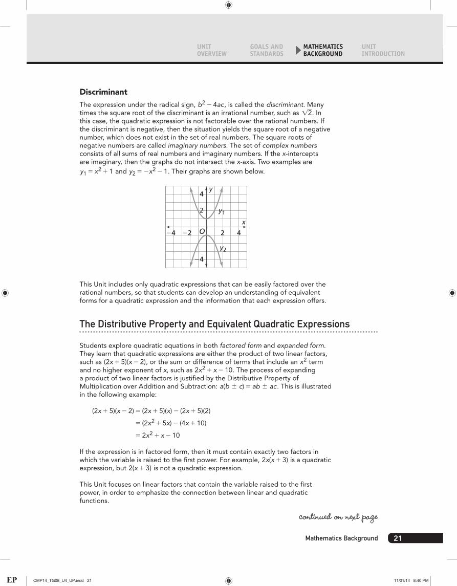
DiscriminantThe expression under the radical sign, b2 - 4ac, is called the discriminant. Many times the square root of the discriminant is an irrational number, such as 12. In this case, the quadratic expression is not factorable over the rational numbers. If the discriminant is negative, then the situation yields the square root of a negative number, which does not exist in the set of real numbers. The square roots of negative numbers are called imaginary numbers. The set of complex numbers consists of all sums of real numbers and imaginary numbers. If the x‑intercepts are imaginary, then the graphs do not intersect the x‑axis. Two examples are y1 = x2 + 1 and y2 = -x2 - 1. Their graphs are shown below.

O

y

y1

y2

−4

−4

−2 42

4

2

x

This Unit includes only quadratic expressions that can be easily factored over the rational numbers, so that students can develop an understanding of equivalent forms for a quadratic expression and the information that each expression offers.

The Distributive Property and Equivalent Quadratic Expressions

Students explore quadratic equations in both factored form and expanded form. They learn that quadratic expressions are either the product of two linear factors, such as (2x + 5)(x - 2), or the sum or difference of terms that include an x2 term and no higher exponent of x, such as 2x2 + x - 10. The process of expanding a product of two linear factors is justified by the Distributive Property of Multiplication over Addition and Subtraction: a(b { c) = ab { ac. This is illustrated in the following example:

(2x + 5)(x - 2) = (2x + 5)(x) - (2x + 5)(2)

= (2x2 + 5x) - (4x + 10)

= 2x2 + x - 10

If the expression is in factored form, then it must contain exactly two factors in which the variable is raised to the first power. For example, 2x(x + 3) is a quadratic expression, but 2(x + 3) is not a quadratic expression.

This Unit focuses on linear factors that contain the variable raised to the first power, in order to emphasize the connection between linear and quadratic functions.



CMP14_TG08_U4_UP.indd 21 11/01/14 8:40 PM


The two factors of a quadratic expression are often binomial expressions or simply binomials. A binomial is an expression with two terms. In this Unit, students do a bit of factoring and multiplying binomials to find equivalent quadratic expressions. For example, you can think of the area of the rectangle below as the product of two linear expressions, the result of multiplying the width by the length. This produces the factored form of a quadratic expression. You can also think of the area as the sum of the areas of the subparts of the rectangle. This generates the expanded form of a quadratic expression. Visit Teacher Place at mathdashboard.com/cmp3 to see the complete animation.

Note that, when using area models, the two figures below represent the same quantity.

x

x

3

1

x

x

3

1

Students often make the mistake of comparing a known length with an unknown length in order to try to determine the value of x. For example, in the first figure above, they may see that five of the 1‑unit lengths fit along the length labeled x. In the second figure above, they may see that two of the 1‑unit lengths fit along the length labeled x. However, since the value of x is unknown from the beginning, its length in an area model cannot be drawn to scale. Be sure to communicate this to students so that they understand that a length of x can actually represent any length, and that the Distributive Property holds for all values of x.

In Say It With Symbols, students address multiplying binomials and factoring quadratic expressions in greater detail.



CMP14_TG08_U4_UP.indd 22 11/01/14 3:25 PM

UNIT OVERVIEW

GOALS AND STANDARDS


UNIT INTRODUCTION

A Note on TerminologyTo introduce quadratic expressions, this Unit uses the term expanded form instead of standard form to help students remember that expanded form represents the sum of the areas of the smaller rectangles that compose the large rectangle. Also, the word standard implies a preferred form. Students should be able to build on prior learning by identifying factored and expanded forms as examples of the Distributive Property, as discussed in earlier Units: Prime Time, Accentuate the Negative, Moving Straight Ahead, and Thinking With Mathematical Models.

This Unit also briefly exposes students to cubic equations, which are either the product of three linear factors, such as y = (x - 2)(x - 2)(x - 2), or a sum or difference of terms that include an x3 term and no higher exponent of x, such as y = x3 - 6x2 + 12x - 8.

Other Contexts for Quadratic Functions

Counting HandshakesThe classic handshake problem and variations on it offer an interesting context for students to explore quadratic functions.

When a team of n members exchanges high fives at the end of a game, how many high fives take place?

Students can draw diagrams, look for patterns in tables, or use reasoning, as follows:

• Each person high fives with (n - 1) people, so there are n(n - 1) high fives. But this counts each high five twice, so you must divide by two. The

number of high fives, h, is h = n(n - 1)2 .

• The first person high fives n - 1 people; the second person high fives n - 2 people, the third person high fives n - 3 people, and so on. The total number of high fives, h, is h = 1 + 2 + 3 + . . . + n - 1.

Sum of the First n Counting NumbersIf both examples of reasoning above are valid, then you can claim that 1 + 2 +

3 + . . . + n - 1 = n(n - 1)2 . This gives a formula for finding the sum of the first n - 1

counting numbers. If you add n to both sides, you have a formula for finding the sum of the first n counting numbers:

1 + 2 + 3 + c + n - 1 + n = n(n - 1)2 + n = n(n + 1)

2

In the ACE for Investigation 3, there is a Did You Know? feature about Carl Gauss, a famous mathematician who discovered this formula when he was a young student. Gauss’ method works for any arithmetic sequence. An arithmetic sequence is a sequence of numbers in which the difference between any two consecutive terms is constant. Below is a generalization of his method.



CMP14_TG08_U4_UP.indd 23 11/01/14 3:25 PM


Generalization of Gauss’s MethodThe sequence of counting numbers, 1, 2, 3, 4, 5, 6, . . . is an arithmetic sequence (the difference is 1); so is the sequence 60, 65, 70, 75, 80, 85, . . . (the difference is 5). Notice that the sequence does not have to start with 1.

For example, here’s how to find the sum of the whole numbers from 1 to 10:

1 + 2 + 3 + 4 + 5+ 6 + 7 + 8 + 9+10

11

11

11

11

11

1 + 2 + 3 + 4 + 5 + 6 + 7 + 8 + 9 + 10 = 5(1 + 10) = 55

Another way to express the sum is n2(first + last), where n is the number of terms being added, “first” is the first number in the sequence, and “last” is the last number in the sequence.

Triangular NumbersTriangular numbers are numbers that can be represented by a triangular array of dots:

1st Figure 2nd Figure 3rd Figure 4th Figure

You can think of each figure as the sum of the first n whole numbers. For example, in the 3rd Figure, the number of dots is 1 + 2 + 3 or 6. In the 4th Figure the number of dots is 1 + 2 + 3 + 4 or 10. The sequence 1, 3, 6, 10, 15, 21, . . . represents triangular numbers. The equation for the nth triangular number is Tn = n(n + 1)

2 . It is similar to the equation for the number of high fives for a team of n members. The number of high fives for n people is actually the (n - 1)th triangular number.

It is interesting for students to observe that the equation y = n(n - 1)2 could

represent the number of high fives, y, that are exchanged among n people; or the (n - 1)th triangular number; or the sum of the first (n - 1) counting numbers. Students encounter triangular numbers again in the Grade 8 Unit Say It With Symbols, when they explore the expression n2 - 1 for odd whole-number values of n. Their results will be the triangular numbers multiplied by 8.



CMP14_TG08_U4_UP.indd 24 05/09/13 5:51 PM

UNIT OVERVIEW

GOALS AND STANDARDS


UNIT INTRODUCTION

The first few contexts in Investigations 1–3 can be represented by equations of the form y = x(x + a) or y = x(a - x). In Investigation 4, students explore classic projectile problems that are represented by y = ax2 + bx + c.

Equations Modeling Projectile MotionEquations such as h = -16t2 + 64t + 6 model one-dimensional projectile motion. They are based on the principles of mechanics. These equations assume that motion occurs in a vacuum, but you can make reasonably accurate predictions about the motion for modest speeds in normal air. The general form is h = 16t2 + v0t + h0. On Earth, the acceleration due to gravity is 32 ft

sec2. In a

context in which upward motion is measured as positive and downward motion is considered negative, we use -32 ft

sec2. The coefficient -16 is half of the Earth’s

gravitational pull on the flying body. v0 is the initial velocity of the projectile, and h0 is the initial height of the projectile.

In the problems involving basketball players, fleas, and frogs jumping, students may bring up the topic of the speed at which the jumpers jump. Speed is associated with change in distance—in this case, a change in height. The jumper’s speed decreases en route to the maximum height and increases on the return trip to the ground. The change in speed is reflected in the tables by the increasingly smaller change in y-value as the x-value increases, until the maximum y-value is reached. At the top of the jump, the speed is 0 for an instant. After the maximum height is attained, y-values decrease by increasing increments, reflecting the change in speed as the jumper returns to the ground.

For example, when the frog jumps, his height is represented by the equation y = -16t2 + 12t + 0.2. The frog is 0.2 feet (or 2.4 inches) tall, so his initial height, or h0, is 0.2. When the frog begins his jump, he takes off at a velocity of 12 feet per second, so v0 is 12. As the frog moves through the air, gravity slows his speed down, until he pauses for an instant at his maximum height. Then, gravity causes the frog to accelerate as he falls back toward the ground. Visit Teacher Place at mathdashboard.com/cmp3 to see the complete animation.



CMP14_TG08_U4_UP.indd 25 05/09/13 5:51 PM


Patterns of change is a unifying theme for looking at linear, exponential, and quadratic functions in Connected Mathematics. As with linear and exponential relationships, students explore the patterns of change that characterize quadratic relationships and learn to recognize these patterns of change in tabular, graphical, or symbolic representations.

Technology: The Use of Calculators

The graphing calculator is used throughout the Unit. Its purpose is to provide students with a useful method for finding information about a situation by examining its graph. In addition, the graphing calculator allows students to look at a lot of examples quickly. This helps students to observe patterns and make conjectures about functions.

Note: The instructions below may not match the particular calculator your students are using.

Graphing Quadratic EquationsGraphing calculators can be used to investigate quadratic functions in much the same way they are used to study linear or exponential functions. The starting point is usually to enter the rule for the function in the menu. Then use the table set menu to determine a starting point and increment for the generation of an (x, y) table and the table command to actually produce the table.

To make a suitable graph for any quadratic, set the window boundaries so that you get a full view of the quadratic shape (and adjust if needed after a first look). Pressing the key will produce a graph that can be traced to read off coordinates of interesting points like intercepts or maximum or minimum points. The viewing window can be magnified around a specific location.

It is important to note that restricting the window to show only values that make sense in a given situation is sometimes useful but can be deceiving. Viewed only in the first quadrant, for example, a parabola that opens upward can seem to be a simple increasing curve. It is often necessary to adjust the window settings to make the characteristic shape apparent. For example, both of the following screens display a graph of the function y = 0.5x2 + 0.2.

As another example, consider the following situation: When one or more of the parameters a, b, or c is held constant while the others are varied, the result is a



CMP14_TG08_U4_UP.indd 26 11/01/14 3:25 PM

UNIT OVERVIEW

GOALS AND STANDARDS


UNIT INTRODUCTION

family of related curves. For example, keeping the coefficient of x2 constant as 2 and varying the values of b and c, we can obtain these graphs:

y = 2x2 + 3x + 4y = 2x2 – x + 6y = 2x2 – 10

These graphs are all exactly the same shape (or “widths”), but they have different locations. With a common viewing window, one could get a misleading impression of those graphs, because the same portion of each graph is not in view or only a piece of each graph is showing.

Adjusting Table SettingsOnce a function has been entered, (x, y) pairs that satisfy the function can be shown in a table. The increments by which the values in a table are displayed can be adjusted by changing the settings in the TABLE SETUP menu.

TABLE SETUP TblStart=0 ∆Tbl=1 Indpnt: Auto Ask Depend: Auto Ask

Press to access the TABLE SETUP menu and enter a new value for △TBL. Then press to display the table. Shown below is a table relating to the function y = x2 + 2x + 4.

X

X=0

012345

Y14712192829



CMP14_TG08_U4_UP.indd 27 11/01/14 3:25 PM


Entering DataIn this Unit, some students may want to look at tables and graphs of values given in tables. Data given as (x, y) pairs can be entered into the calculator and plotted.

To enter a list of (x, y) data pairs, press to access the STAT EDIT menu. Press to select the Edit mode. Then, enter the data pairs into the L1 and L2 columns: enter the first number, press , and use the arrow keys to move to the L2 column. Continue until all the data pairs have been entered. For example, you might enter the following data pairs:

L1

L1(l)=0

012345

L2028183250

L3---------

Plotting PointsTo plot the data you have entered, use the STAT PLOT menu. Use the arrow keys and to move around in the screen and to highlight the elements (ON, , L1, L2, and )

STAT PLOTS 1: Plot1...ON 2: Plot2...ON 3: Plot3...ON

4 PlotsOFF

L1 L2

L1 L2

L1 L2

Plot1 Plot2 Plot3 On Off Type: Xlist: L1 Ylist: L2 Mark: + .

Next, press , which will display a screen similar to that shown below. To accommodate the data you input, adjust the window settings by entering values and pressing , allowing some margin beyond for data points if possible. Then, press .

WINDOW Xmin=0 Xmax=10 X:scl=1 Ymin=0 Ymax=60 Yscl=10 Xres=1



CMP14_TG08_U4_UP.indd 28 05/09/13 5:51 PM

Representing Quadratic Functions With Equations · Representing Quadratic Functions With Equations...

Documents

Transcript of Representing Quadratic Functions With Equations · Representing Quadratic Functions With Equations...