Representing Groundwater in Management Models

Julien Harou

University College London

2010 International Congress on Environmental Modelling and Software

July 4-8 2010 Ottawa, Canada

D5

SR

-4

SR

-1D

94&D

40

D76b

D77

D73

D66

SR

-3

Kesw

ick R

eservoir

Clair E

ngle Lake

Shasta Lake

Whiskeytow

n Lake

D30

D31

D61

CL

EA

R C

RE

EK

TR

INIT

Y

RIV

ER

LE

WIS

TO

N L

AK

E

INF

LO

W

CO

TT

ON

WO

OD

C

RE

EK

TH

OM

ES

&

EL

DE

R C

RE

EK

S

DA

58

LO

CA

L W

AT

ER

S

UP

PL

Y IN

C. C

OW

C

RE

EK

& B

AT

TL

E C

RE

EK

AN

TE

LO

PE

, M

ILL

,DR

Y,D

EE

R

& B

IG C

HIC

O

CR

EE

KS

DA

15

Sac W

est R

efuges

LA

KE

SH

AS

TA

IN

FL

OW

D74

CV

PM

2S

Black B

utte Lake

ST

ON

Y

CR

EE

K

C4

GW

-1

CV

PM

1S

C3

CV

PM

1G

GW

-2

C6

CV

PM

2G

C12

C69

GW

-3

C13

CV

PM

3S

C15

GW

-4

C14

CV

PM

4S

CV

PM

4G

Glenn-Colusa Canal

Colusa B

asin Drain

Redding

C5

Clear CreekTunnel

DA

10

GW

-1

GW

-2

GW

-3

GW

-4

Spring Creek Power Conduit

SR

-BB

L

Trinity R

iver Minim

um

Flow

s

D75

C301

DA

15

D76a

C11

C303

C1

Tehema-Colusa CanalCorning Canal

Misc Left & Right Bank Diversions

Knights Landing

Ridge C

ut

C304

C305

C302

DA

12

loc

al

wa

ter

C2

DA

12D

A 10

DA

58

DA

15

CV

PM

2 U

rban

CV

PM

3 U

rban

CV

PM

4 U

rban

GW

-1

DA

11

C9

C81

C82

DA

10

LO

CA

L

WA

TE

R S

UP

PL

Y

C86

DA

5

PA

YN

ES

AN

D

SE

VE

N M

ILE

C

RE

EK

S

C87

DA

12

CV

PM

3G

T41

T42

SIN

K to

R

eg

ion

2

SIN

K to

R

eg

ion

2

SIN

K to

R

eg

ion

2

C313

HU

S1D

5

HU

S1S

R3

HU

S1D

74

HU

1

HS

D1

HG

D1

HU

S2C

1

HU

S2D

77

HU

S2C

11

HU

S2C

9

HU

2

HS

D2

HU

S3C

11

HU

S3C

13

HG

D2

HU

S3C

305

HU

S3D

66

HS

UR

C303

HU

3

HS

D3

HG

D3

HU

S4D

30

HU

S5D

31

HU

4

HS

D4

HG

D4

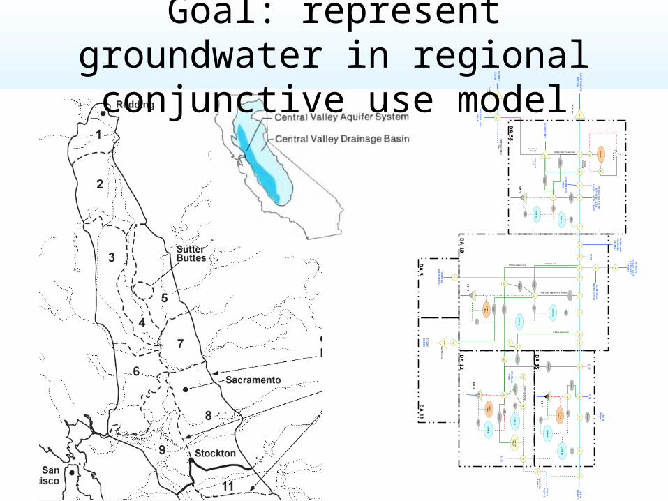
Goal: represent groundwater in regional conjunctive use model

CV-RASA1 USGS Groundwater Model (1989)

• Finite-Difference Groundwater model: 529 100 km2 cells, 4 layers• Upscaling: vertical aggregation into 1 layer model by summing depth-average transmissivity and storage coefficient parameters

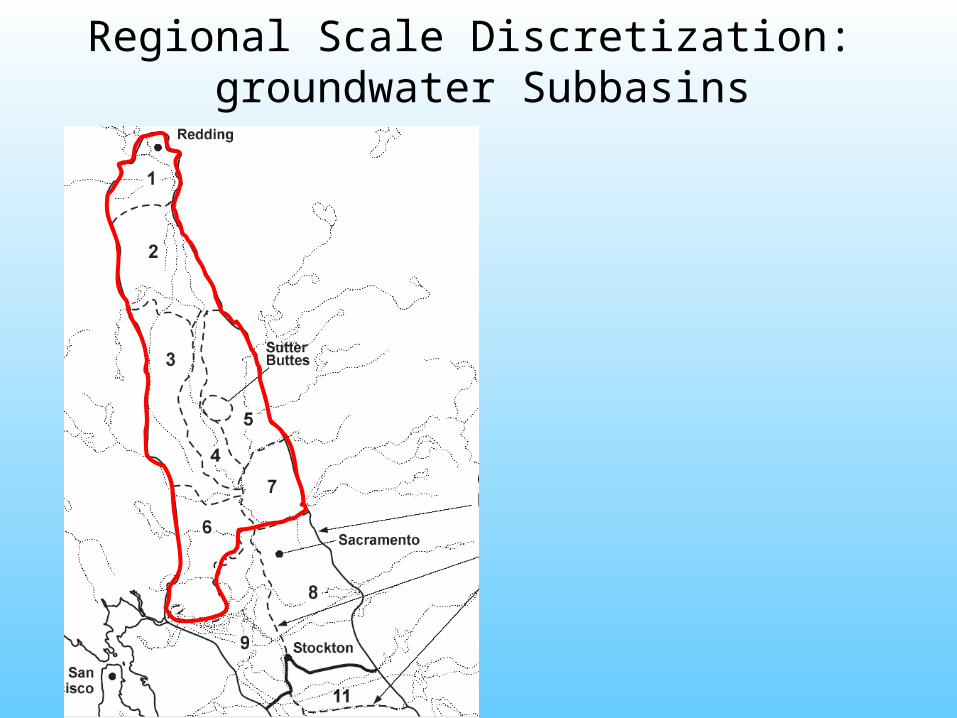
Regional Scale Discretization: groundwater Subbasins

12

34

56

78

910

1112

1314

1516

1718

19

2021

2223

2425

2627

2829

3031

3233

3435

3637

3839

4041

42

4344

4546

4748

4950

5152

5354

5556

5758

5960

6162

6364

6566

6768

6970

7172

7374

7576

7778

7980

8182

8384

8586

87

8889

9091

9293

9495

9697

9899

100101

102103

104105

106107

108

109110

111112

113114

115116

117118

119120

121122

123124

125126

127128

129130

131132

133134

135136

137138

139

140141

142143

144145

146147

148149

150151

152

153154

155156

157158

159160

161

162163

164165

166

167

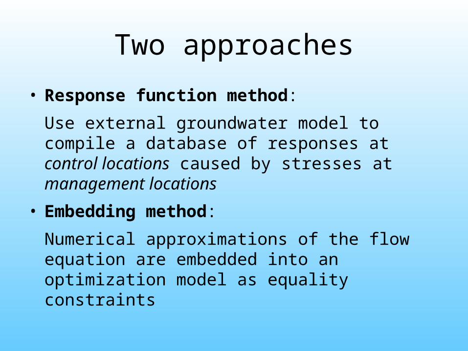
Two approaches

• Response function method:

Use external groundwater model to compile a database of responses at control locations caused by stresses at management locations

• Embedding method:

Numerical approximations of the flow equation are embedded into an optimization model as equality constraints

Embedding 3 groundwater model formulations

1. Sequential time-marching method (STM)

Implicit scheme finite-difference groundwater model, analogous to MODFLOW

2. Eigenvalue method (EV)

Efficient numerical scheme solves spatially discretized but time-continuous version of groundwater flow partial differential equations; allows aggregation into control variables (e.g. mean head per sub-basin)

3. Storage coefficient method (SC)

Storage coefficient equation relates volume of water released (or absorbed) from (into) storage per unit surface area of aquifer per unit change in hydraulic head.

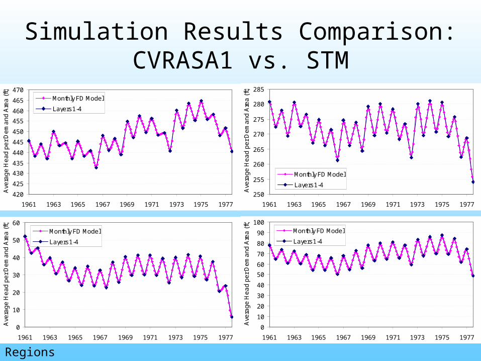
Simulation Results Comparison:CVRASA1 vs. STM

420

425

430

435

440

445

450

455

460

465

470

1961 1963 1965 1967 1969 1971 1973 1975 1977

Ave

rag

e H

ea

d p

er

De

ma

nd

Are

a (

ft)

Monthly FD Model

Layers1-4

250

255

260

265

270

275

280

285

1961 1963 1965 1967 1969 1971 1973 1975 1977

Ave

rag

e H

ea

d p

er

De

ma

nd

Are

a (

ft)

Monthly FD Model

Layers1-4

0

10

20

30

40

50

60

1961 1963 1965 1967 1969 1971 1973 1975 1977

Ave

rag

e H

ea

d p

er

De

ma

nd

Are

a (

ft)

Monthly FD Model

Layers1-4

0

10

20

30

40

50

60

70

80

90

100

1961 1963 1965 1967 1969 1971 1973 1975 1977

Ave

rag

e H

ea

d p

er

De

ma

nd

Are

a (

ft)

Monthly FD Model

Layers1-4

Regions 1,2,4,5

Simulation Results Comparison:CVRASA1 vs. EV

Regions 1,2,4,5

420

425

430

435

440

445

450

455

460

465

470

1961 1963 1965 1967 1969 1971 1973 1975 1977

Ave

rag

e H

ea

d p

er

De

ma

nd

Are

a (

ft)

EV

Layers1-4

250

255

260

265

270

275

280

285

1961 1963 1965 1967 1969 1971 1973 1975 1977

Ave

rag

e H

ea

d p

er

De

ma

nd

Are

a (

ft)

EV

Layers1-4

0

10

20

30

40

50

60

1961 1963 1965 1967 1969 1971 1973 1975 1977

Ave

rag

e H

ea

d p

er

De

ma

nd

Are

a (

ft)

EV

Layers1-4

0

10

20

30

40

50

60

70

80

90

100

1961 1963 1965 1967 1969 1971 1973 1975 1977

Ave

rag

e H

ea

d p

er

De

ma

nd

Are

a (

ft)

EV

Layers1-4

EV method using 9 control variables, 9 basic stresses.

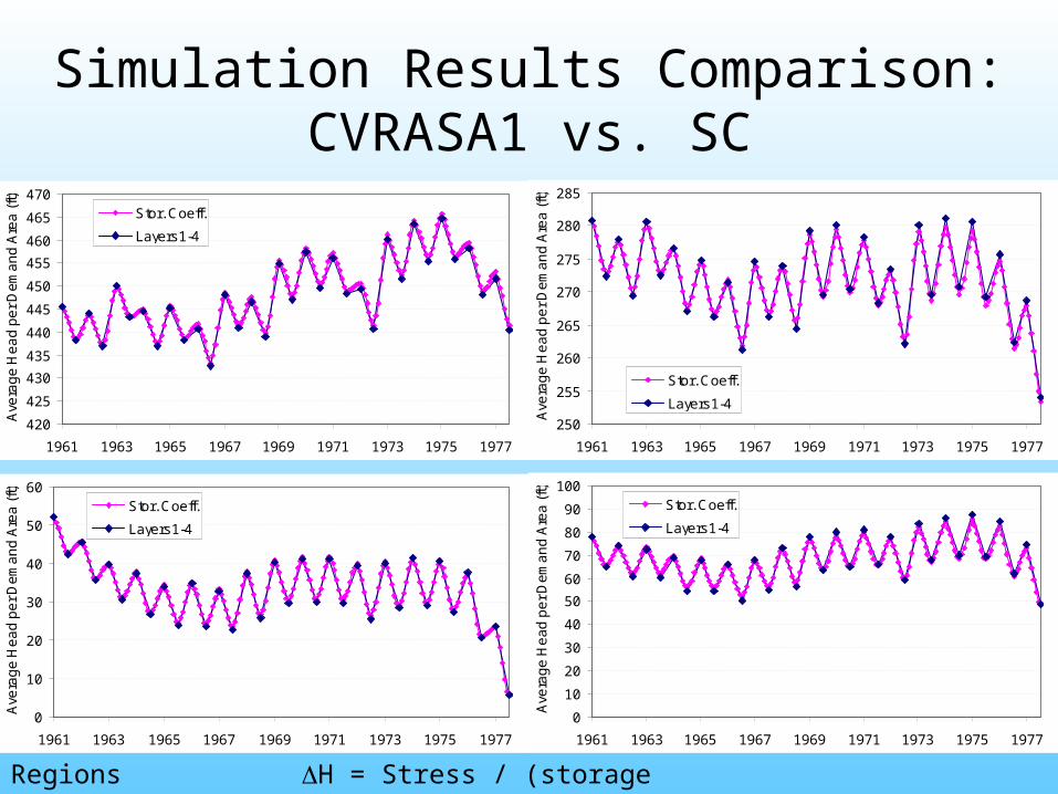
Simulation Results Comparison:CVRASA1 vs. SC

Regions 1,2,4,5

420

425

430

435

440

445

450

455

460

465

470

1961 1963 1965 1967 1969 1971 1973 1975 1977

Ave

rag

e H

ea

d p

er

De

ma

nd

Are

a (

ft)

Stor. Coeff.

Layers1-4

250

255

260

265

270

275

280

285

1961 1963 1965 1967 1969 1971 1973 1975 1977

Ave

rag

e H

ea

d p

er

De

ma

nd

Are

a (

ft)

Stor. Coeff.

Layers1-4

0

10

20

30

40

50

60

1961 1963 1965 1967 1969 1971 1973 1975 1977

Ave

rag

e H

ea

d p

er

De

ma

nd

Are

a (

ft)

Stor. Coeff.

Layers1-4

0

10

20

30

40

50

60

70

80

90

100

1961 1963 1965 1967 1969 1971 1973 1975 1977

Ave

rag

e H

ea

d p

er

De

ma

nd

Are

a (

ft)

Stor. Coeff.

Layers1-4

H = Stress / (storage coeff. * area)

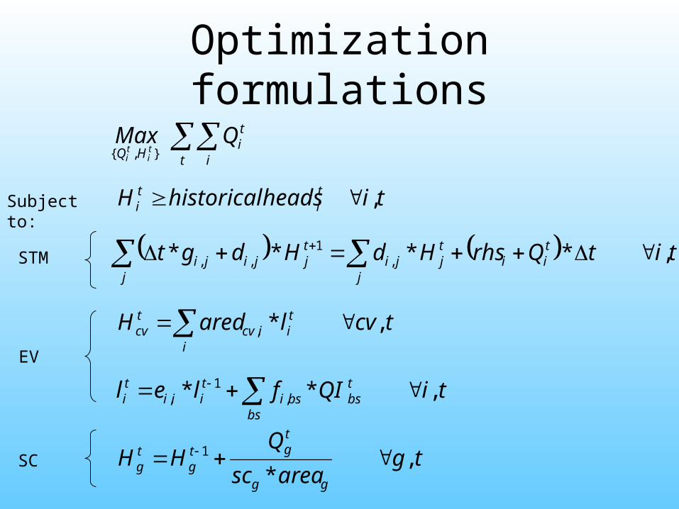
Optimization formulations

t i

ti

HQQMax

ti

ti },{

tiheadshistoricalH ti

ti ,

titQrhsHdHdgt tii

j

tjji

j

tjjiji ,**** ,

1,,

tcvlaredHi

tiicv

tcv ,*,

tiQIflelbs

tbsbsi

tiii

ti ,** ,

1,

tgareasc

QHH

gg

tgt

gtg ,

*1

Subject to:

STM

EV

SC

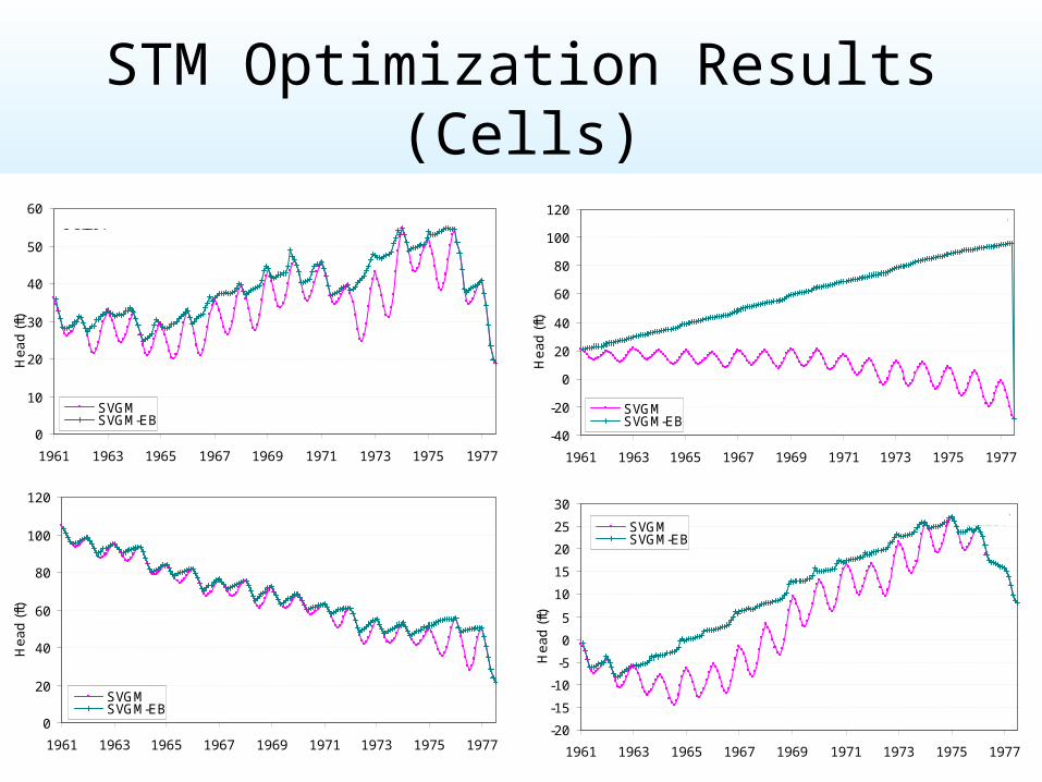
STM Optimization Results (Cells)

0

10

20

30

40

50

60

1961 1963 1965 1967 1969 1971 1973 1975 1977

He

ad

(ft)

SVGMSVGM-EB

Cell 97

-40

-20

0

20

40

60

80

100

120

1961 1963 1965 1967 1969 1971 1973 1975 1977

He

ad

(ft)

SVGMSVGM-EB

Cell 107

0

20

40

60

80

100

120

1961 1963 1965 1967 1969 1971 1973 1975 1977

He

ad

(ft)

SVGMSVGM-EB

Cell 132

-20

-15

-10

-5

0

5

10

15

20

25

30

1961 1963 1965 1967 1969 1971 1973 1975 1977

He

ad

(ft)

SVGMSVGM-EB

Cell 137

EV Optimization Results (Basins)

0

50

100

150

200

250

300

350

1961 1963 1965 1967 1969 1971 1973 1975 1977

Ave

rag

e H

ea

d p

er

Su

bb

asi

n (

ft)

SVGMSVGM-EV

Subbasin 4

0

100

200

300

400

500

600

700

800

1961 1963 1965 1967 1969 1971 1973 1975 1977

Ave

rag

e H

ea

d p

er

Su

bb

asi

n (

ft)

SVGMSVGM-EV

Subbasin 7

40

60

80

100

120

140

160

1961 1963 1965 1967 1969 1971 1973 1975 1977

Ave

rag

e H

ea

d p

er

Su

bb

asi

n (

ft)

SVGMSVGM-EV

Subbasin 5

25

45

65

85

105

125

145

1961 1963 1965 1967 1969 1971 1973 1975 1977

Ave

rag

e H

ea

d p

er

Su

bb

asi

n (

ft)

SVGMSVGM-EV

Subbasin 8

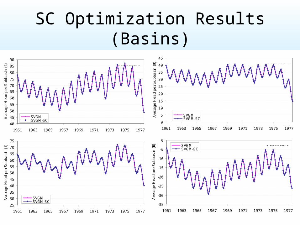
SC Optimization Results (Basins)

40

45

50

55

60

65

70

75

80

85

90

1961 1963 1965 1967 1969 1971 1973 1975 1977

Ave

rag

e H

ea

d p

er

Su

bb

asi

n (

ft)

SVGMSVGM-SC

Subbasin 5

0

5

10

15

20

25

30

35

40

45

1961 1963 1965 1967 1969 1971 1973 1975 1977

Ave

rag

e H

ea

d p

er

Su

bb

asi

n (

ft)

SVGMSVGM-SC

Subbasin 6

25

30

35

40

45

50

55

60

65

70

75

1961 1963 1965 1967 1969 1971 1973 1975 1977

Ave

rag

e H

ea

d p

er

Su

bb

asi

n (

ft)

SVGMSVGM-SC

Subbasin 8

-35

-30

-25

-20

-15

-10

-5

0

1961 1963 1965 1967 1969 1971 1973 1975 1977

Ave

rag

e H

ea

d p

er

Su

bb

asi

n (

ft) SVGMSVGM-SC

Subbasin 9

Computational Comparison

MATLAB GAMS Simulation Simulation Optimization

Sequential time-marching (STM) method

0.72 sec. stable

7.2 sec. stable

3.6 min. moderate stability

Eigenvalue (EV) method

~ 0.02 sec. stable

3.4 sec. stable

2.9 min. (init. sol.) poor stability

Storage coefficient (SC) method

~ 0.01 sec. stable

0.003 sec. stable

0.003 sec. stable

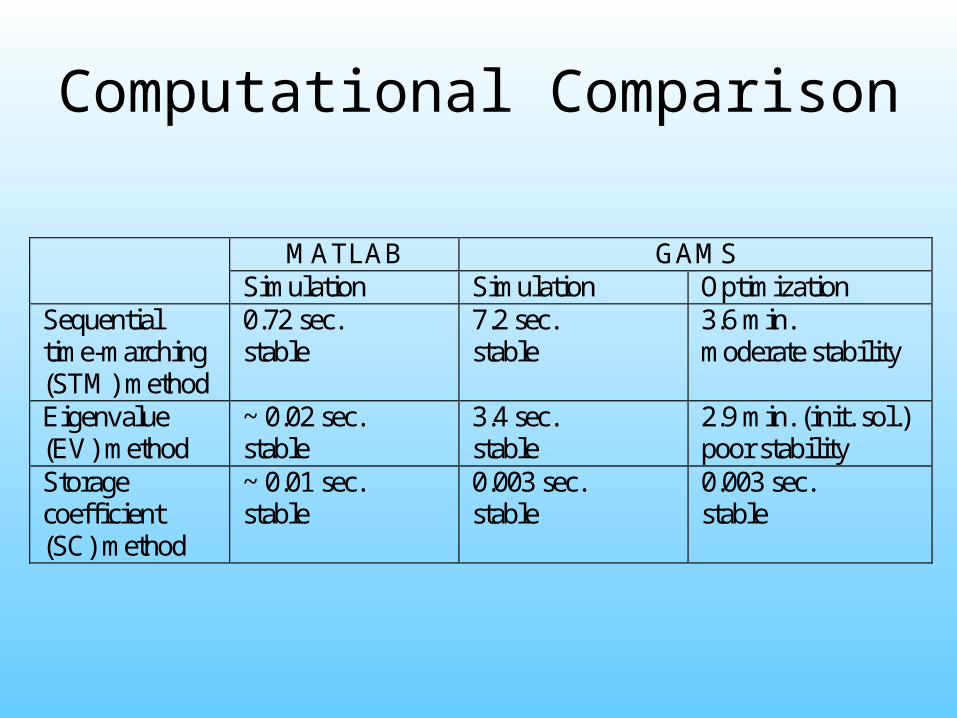
Computational Comparison

MATLAB GAMS Simulation Simulation Optimization

Sequential time-marching (STM) method

0.72 sec. stable

7.2 sec. stable

3.6 min. moderate stability

Eigenvalue (EV) method

~ 0.02 sec. stable

3.4 sec. stable

2.9 min. (init. sol.) poor stability

Storage coefficient (SC) method

~ 0.01 sec. stable

0.003 sec. stable

0.003 sec. stable

Conclusions

• Groundwater simulation can efficiently be included in management models, particularly if only flows or heads in certain cells or aggregations of cells are of interest

• Optimization can be problematic:

Embedding spatially discretized groundwater models in mathematical program constraint sets can lead to significant numerical errors