
REPRESENTATIONS OF FUNCTIONS HARMONIC IN THE UPPER … › download › pdf › 52939691.pdf · of...
79
REPRESENTATIONS OF FUNCTIONS HARMONIC IN THE UPPER HALF-PLANE AND THEIR APPLICATIONS a dissertation submitted to the department of mathematics and the institute of engineering and science of bilkent university in partial fulfillment of the requirements for the degree of doctor of philosophy By Se¸ cil Gerg¨ un September, 2003
Transcript of REPRESENTATIONS OF FUNCTIONS HARMONIC IN THE UPPER … › download › pdf › 52939691.pdf · of...
REPRESENTATIONS OF FUNCTIONSHARMONIC IN THE UPPER HALF-PLANE
AND THEIR APPLICATIONS
a dissertation submitted to
the department of mathematics
and the institute of engineering and science
of bilkent university
in partial fulfillment of the requirements
for the degree of
doctor of philosophy
By
Secil Gergun
September, 2003
I certify that I have read this thesis and that in my opinion it is fully adequate,
in scope and in quality, as a dissertation for the degree of doctor of philosophy.
Prof. Dr. Iossif V. Ostrovskii(Supervisor)
I certify that I have read this thesis and that in my opinion it is fully adequate,
in scope and in quality, as a dissertation for the degree of doctor of philosophy.
Prof. Dr. Mefharet Kocatepe
I certify that I have read this thesis and that in my opinion it is fully adequate,
in scope and in quality, as a dissertation for the degree of doctor of philosophy.
Assoc. Prof. Dr. Turgay Kaptanoglu
ii

I certify that I have read this thesis and that in my opinion it is fully adequate,
in scope and in quality, as a dissertation for the degree of doctor of philosophy.
Asst. Prof. Dr. Alexander Goncharov
I certify that I have read this thesis and that in my opinion it is fully adequate,
in scope and in quality, as a dissertation for the degree of doctor of philosophy.
Asst. Prof. Dr. Ozgur Oktel
Approved for the Institute of Engineering and Science:
Prof. Dr. Mehmet B. BarayDirector of the Institute
iii

ABSTRACT
REPRESENTATIONS OF FUNCTIONS HARMONIC INTHE UPPER HALF-PLANE AND THEIR
APPLICATIONS
Secil Gergun
Ph.D. in Mathematics
Supervisor: Prof. Dr. Iossif V. Ostrovskii
September, 2003
In this thesis, new conditions for the validity of a generalized Poisson represen-
tation for a function harmonic in the upper half-plane have been found. These
conditions differ from known ones by weaker growth restrictions inside the half-
plane and stronger restrictions on the behavior on the real axis.
We applied our results in order to obtain some new factorization theorems in
Hardy and Nevanlinna classes.
As another application we obtained a criterion of belonging to the Hardy class
up to an exponential factor.
Finally, our results allowed us to extend the Titchmarsh convolution theorem
to linearly independent measures with unbounded support.
Keywords: Analytic curves, generalized Poisson integral, Hardy class, Nevanlinna
class, Nevanlinna characteristics, Titchmarsh convolution theorem.
iv
OZET
UST YARI DUZLEMDEKI HARMONIKFONKSIYONLARIN GOSTERIMLERI VE BUNLARIN
UYGULAMALARI
Secil Gergun
Matematik, Doktora
Tez Yoneticisi: Prof. Dr. Iossif V. Ostrovskii
Eylul, 2003
Bu tezde ust yarı duzlemdeki harmonik fonksiyonların genellestirilmis Poisson
integrali biciminde gosterilebilmelerinin yeni kosullarını bulduk. Bu kosullar, ust
yarı duzlemde daha zayıf buyume sınırlandırmaları ve reel eksende daha kuvvetli
sınırlandırmalarla bilinen kosullardan farklılık gosterirler.
Sonuclarımızı, Hardy ve Nevanlinna sınıflarına, bu sınıflarda yeni faktorizas-
yon teoremleri bulmak icin uyguladık.
Diger bir uygulama olarak, fonksiyonların bir ustel carpanla birlikte Hardy
sınıfına ait olmalarının bir kriterini bulduk.
Son olarak, sonuclarımız Titchmarsh’ın konvolusyon teoremini sonsuz daya-
naklı, lineer bagımlı olcumlere genisletmemize olanak sagladı.
Anahtar sozcukler : Analitik egriler, genellestirilmis Poisson integrali, Hardy
sınıfı, Nevanlinna sınıfı, Nevanlinna karakteristikleri, Titchmarsh’ın konvolusyon
teoremi.
v

Acknowledgement
I would like to express my deep gratitude to my supervisor Prof. Iossif
Vladimirovich Ostrovskii for his excellent guidance, valuable suggestions, encour-
agements, and patience.
I am also grateful to Bilsel Alisbah for establishing the Orhan Alisbah Fel-
lowship. I also thank to the committee members for naming me the recipient of
award.
I want to thank Alexander Iljinskii, Alexander Ulanovskii and Natalya Zhel-
tukhina for careful reading of some parts of the text and valuable remarks.
My special thanks go to my parents Sevil and Mehmet Gergun, my sister Serpil
Gergun and my husband Salim Oflaz for their encouragements and supports.
I would also like to thank my friends for their encouragements and supports.
vi

Contents
1 Introduction 1
2 Statement of results 4
2.1 Generalized Poisson representation of a function harmonic in the
upper half-plane . . . . . . . . . . . . . . . . . . . . . . . . . . . . 4
2.2 Applications to Hardy and Nevanlinna classes . . . . . . . . . . . 8
2.3 Application to generalization of the Titchmarsh convolution theorem 12
3 Preliminaries 15
3.1 Generalized Poisson integral . . . . . . . . . . . . . . . . . . . . . 15
3.2 Blaschke products . . . . . . . . . . . . . . . . . . . . . . . . . . . 22
3.3 Hardy classes and the Nevanlinna class . . . . . . . . . . . . . . . 23
3.4 Carleman’s and Nevanlinna’s formulas . . . . . . . . . . . . . . . 25
3.5 Compactness Principle for harmonic functions . . . . . . . . . . . 26
3.6 Nevanlinna characteristics . . . . . . . . . . . . . . . . . . . . . . 26
3.7 Titchmarsh convolution theorem . . . . . . . . . . . . . . . . . . . 28
vii

CONTENTS viii
4 Auxiliary results 30
4.1 Estimates for means of Blaschke products and Poisson integrals . 30
4.2 A representation theorem . . . . . . . . . . . . . . . . . . . . . . . 34
4.3 A criterion of belonging to H∞(C+) up to an exponential factor
for functions of the Nevanlinna class . . . . . . . . . . . . . . . . 37
5 Generalized Poisson representation of a function harmonic in the
upper half-plane 39
5.1 A weakened version of the main result on representation of a har-
monic function by a generalized Poisson integral . . . . . . . . . . 39
5.2 A local representation of a harmonic function by a generalized
Poisson kernel . . . . . . . . . . . . . . . . . . . . . . . . . . . . . 43
5.3 Harmonic functions with growth restrictions on two horizontal lines 46
5.4 Main result on representation of harmonic functions by generalized
Poisson integrals . . . . . . . . . . . . . . . . . . . . . . . . . . . 49
6 Applications to the Hardy and the Nevanlinna classes 54
6.1 Factorization in the Nevanlinna class . . . . . . . . . . . . . . . . 54
6.2 Factorization in H∞(C+) when the factors are connected by a lin-
ear equation . . . . . . . . . . . . . . . . . . . . . . . . . . . . . . 58
6.3 A criterion of belonging to Hp(C+) up to an exponential factor . . 61
7 Application to generalization of the Titchmarsh convolution the-
orem 66

Chapter 1
Introduction
It is well-known from Complex Analysis that if a function u is harmonic in the
disk DR := z ∈ C : |z| < R and continuous on its closure, then u admits the
following Poisson representation
u(z) =1
2π
∫ 2π
0
R2 − r2
R2 − 2Rr cos(θ − ϕ) + r2u(Reiθ)dθ, z = reiϕ ∈ DR.
The counterpart of this representation for the upper half-plane C+ := z ∈C : Im z > 0 is the following:
u(z) =y
π
∫ ∞
−∞
u(t)
(x− t)2 + y2dt, z = x + iy ∈ C+. (1.1)
Unfortunately, this representation does not hold generally for functions harmonic
in C+, and continuous on its closure C+ := z ∈ C : Im z ≥ 0, even if the
integral on the right hand side converges. For example, take u as the imaginary
part of any polynomial with real coefficients. The conditions for the validity of
representation (1.1) are rather restrictive; roughly speaking, they are of the kind
u(z) = o(|z|), |z| → ∞.
The following more general representation
u(z) =y
π
∫ ∞
−∞
dν(t)
(x− t)2 + y2+ cy, z = x + iy ∈ C+, (1.2)
1

CHAPTER 1. INTRODUCTION 2
of a harmonic function u in C+, where ν is a σ-finite Borel measure on R and c is
a constant, is also very important and has applications in the theory of integral
transforms [2, Ch.4], in the theory of entire functions [19, Part II], [18, Ch.5], [17,
Ch.3], in the theory of Hp spaces [16, Ch.6].
It is well-known (see, e.g. [16, p.107], [19, p.100]) that (1.2) holds if and only
if u can be represented in the form u = u1−u2 where u1 and u2 are non-negative
harmonic functions in C+. Nevertheless, for several applications (see, e.g. [17,
Ch.3], [18, Ch.5]) conditions that can be expressed in terms of the growth of u
are more useful. For a function u continuous on C+ the strongest result of this
kind was obtained by R. Nevanlinna [21].
The present thesis is devoted to the conditions of the validity of a more general
representation, including (1.2) as a special case, and some of its applications.
This representation has the form
u(z) =
∫ ∞
−∞Pq(z, t)dν(t) + ImP (z), z ∈ C+. (1.3)
Here Pq(z, t) is the generalized Poisson kernel defined by the formula
Pq(z, t) = Im
1
π
(1 + tz)q
(t− z)(1 + t2)q
, q ∈ N ∪ 0,
the measure ν is a σ-finite Borel measure on R, and P is a polynomial of degree
at most q. Note that, if we put q = 1 in (1.3), we obtain the representation (1.2).
The representation (1.3) for u being continuous in C+ was first considered by R.
Nevanlinna [21].
R. Nevanlinna [21] and later N. Govorov [14] showed that representation (1.3)
is valid under a growth condition on u in the upper half-plane, and a condition
on the behavior of u near the real line. Our results differ from the cited ones by
a remarkably relaxed growth condition in the upper half-plane.
We applied our results on representation of harmonic function in upper half-
plane to obtain some new factorization theorems in Hardy and Nevanlinna classes.
The classical factorization theorems in Hardy and Nevanlinna classes [7,

CHAPTER 1. INTRODUCTION 3
Ch.11], [15, Ch.8], [16, Ch. VI], are well-known and have plenty of applica-
tions in Complex Analysis and Functional Analysis [7, 15, 16, 19]. In 1985, I.V.
Ostrovskii [23] proved a factorization theorem in the Hardy class H∞(C+) of a
different kind. This theorem was a basis of his extension [23] of the Titchmarsh
convolution theorem to measures with unbounded support.
In this thesis, we applied the theorem on the representation of harmonic func-
tions in the upper half-plane to obtain a factorization theorem which improves
and extends the mentioned theorem of [23] in several manners. One of them is an
improvement of the theorem in the case when the factors are linearly dependent.
The last result is used to get a counterpart of the result of [23] for the linearly
dependent measures with unbounded support.
We also applied the representation theorem to obtain a criterion of belonging
to the Hardy class Hp(C+) up to an exponential factor.
The results of this thesis have been published [8], [9], [11], [12] and accepted
[10] for publication.
Chapter 2
Statement of results
2.1 Generalized Poisson representation of a
function harmonic in the upper half-plane
In this thesis we found some conditions of the validity of the following represen-
tation of a real-valued harmonic function u in C+:
u(z) =
∫ ∞
−∞Pq(z, t)dν(t) + Im P (z), z ∈ C+, (2.1)
where Pq(z, t) is the generalized Poisson kernel defined by the formula
Pq(z, t) = Im
1
π
(1 + tz)q
(t− z)(1 + t2)q
, q ∈ N ∪ 0,
ν is a σ-finite Borel measure on R satisfying∫ ∞
−∞
d|ν|(t)1 + |t|q+1
< ∞,
and P is a real polynomial of degree at most q.
Further, we assume that all harmonic functions and Borel measures are real-
valued.
For functions u harmonic in C+ and continuous in C+, R. Nevanlinna gives
the strongest result on the validity of the representation (2.1):
4

CHAPTER 2. STATEMENT OF RESULTS 5
Theorem A ([21]) Let u be a function harmonic in C+, continuous in C+ and
satisfying the conditions:
(i) There exists a sequence rk, rk →∞, such that∫ π
0
u+(reiθ) sin θdθ = O(rq), r = rk →∞, (2.2)
(ii) ∫ ∞
−∞
u+(t)
1 + |t|q+1dt < ∞. (2.3)
Then u admits representation (2.1) with dν(t) = u(t)dt.
In [14], N. V. Govorov showed that the continuity assumption in the closed
half- plane can be dropped under some condition:
Theorem B ([14]) Let u be a function harmonic in C+, if
max0<θ<π
u+(reiθ) = O(rα), for some α, α < q, (2.4)
then u admits representation (2.1).
Our main result is the following:
Theorem 2.1 Let u be a function harmonic in C+ and satisfying the following
conditions:
(i) There exists a sequence rk, rk →∞, such that∫ π
0
u+(reiθ) sin θdθ ≤ expo(r), r = rk →∞. (2.5)
(ii) There exists α > 0 such that
lim infs→0+
∫ ∞
−∞
|u(t + is)|1 + |t|α
dt < ∞. (2.6)

CHAPTER 2. STATEMENT OF RESULTS 6
Then u admits representation (2.1) where q = maxn ∈ N ∪ 0 : n < α, ν
is a σ-finite Borel measure on R satisfying∫ ∞
−∞
d|ν|(t)1 + |t|α
< ∞,
and P is a real polynomial of degree at most q.
Note that Nevanlinna’s [21] and Govorov’s [14] results, mentioned above, are
not contained in Theorem 2.1 because neither (2.3) nor (2.4) imply (2.6), and our
result differs from the Nevalinna’s and Govorov’s results by much weaker growth
condition (2.5) on the upper half-plane comparatively with (2.2) and (2.4).
The following immediate corollary of Theorem 2.1, gives the conditions of
validity of usual Poisson representation of a function harmonic in C+.
Corollary 2.2 Let u be a function harmonic in C+ and satisfying the following
conditions:
(i) There exists a sequence rk, rk →∞, such that∫ π
0
u+(reiθ) sin θdθ ≤ expo(r), r = rk →∞, (2.7)
(ii)
lim infs→0+
∫ ∞
−∞
|u(t + is)|1 + t2
dt < ∞. (2.8)
Then u admits representation
u(z) =y
π
∫ ∞
−∞
dν(t)
(x− t)2 + y2+ cy, z = x + iy ∈ C+, (2.9)
where ν is a σ-finite Borel measure on R satisfying∫ ∞
−∞
d|ν|(t)1 + t2
< ∞,
and c is a real constant.

CHAPTER 2. STATEMENT OF RESULTS 7
Assumptions (2.5) and (2.6) in Theorem 2.1 are sharp in the following sense:
“o” cannot be replaced by “O” in (2.5) as the example u(z) = Recos z shows.
Moreover, (2.6) cannot be replaced by∫ ∞
−∞
|u(t + iH)|1 + |t|α
dt < ∞,
for some H > 0. This follows from the example u(z) = Im(z − iH)2n, n >
(α− 1)/2, n ∈ N. It is also worth mentioning that |u(t + is)| cannot be replaced
with u+(t+ is) in (2.6) as the example u(z) = −Rez2n, n > (α− 1)/2, n ∈ N,
shows.
We also considered the possibility of weakening the condition (2.6) in Theorem
2.1. For example, is it possible to replace (2.6) by a condition requiring conver-
gence of the integrals in (2.6) only over two horizontal lines? In some sense, there
is an affirmative answer to this question. To formulate our result more precisely,
we need a lemma.
Lemma 2.3 Let u(z) be a function harmonic in C+ and satisfying the following
condition:
∃H > 0, ∀R > 0, sup0<y<H
∫ R
−R
|u(x + iy)|dx < ∞. (2.10)
Then there exists a Borel measure ν on R such that for all R > 0 it satisfies
|ν|([−R,R]) < ∞, and the function
u(z)−∫ R
−R
Pq(z, t)dν(t), q ∈ N ∪ 0,
is harmonic in C+, continuous in C+ ∪ (−R,R) and vanishes on (−R,R).
Our next result is the following:
Theorem 2.4 Let u be a function harmonic in C+ satisfying condition (2.10) of
Lemma 2.3 and (2.5) of Theorem 2.1. Assume additionally that u satisfies the
following condition:
There exist H > 0 and α > 0 such that∫ ∞
−∞
|u(t + iH)|1 + |t|α
dt +
∫ ∞
−∞
d|ν|(t)1 + |t|α
< ∞, (2.11)
CHAPTER 2. STATEMENT OF RESULTS 8
where ν is the σ-finite Borel measure defined in Lemma 2.3.
Then u admits representation (2.1), where q and P are as in Theorem 2.1.
The following corollary to Theorem 2.4 is immediate.
Corollary 2.5 Let u be a function harmonic in C+, continuous in C+ and sat-
isfying (2.5) of Theorem 2.1. Suppose there exist H > 0 and α > 0 such that∫ ∞
−∞
|u(t)|+ |u(t + iH)|1 + |t|α
dt < ∞. (2.12)
Then u admits representation (2.1) with dν(t) = u(t)dt, where q and P are
as in Theorem 2.1.
In Chapter 5, we will prove a weakened version of Theorem 2.1 where condition
(2.6) is replaced by a stronger one, then we will prove Lemma 2.3 and Theorem
2.4. Finally, we will prove Theorem 2.1 using its weakened version and Theorem
2.4.
2.2 Applications to Hardy and Nevanlinna
classes
The Hardy class Hp(C+), 0 < p ≤ ∞, consists of all functions f analytic in the
upper half-plane C+ and satisfying the condition
sup0<y<∞
‖f(·+ iy)‖p < ∞,
where
‖h(·)‖p =(∫∞
−∞ |h(x)|pdx)min(1,1/p)
, 0 < p < ∞,
‖h(·)‖∞ = ess supx∈R |h(x)|.
In 1985, I.V. Ostrovskii [23] proved the following factorization theorem in
the Hardy class H∞(C+). This theorem was a basis of his extension [23] of the
Titchmarsh convolution theorem to measures with unbounded support.

CHAPTER 2. STATEMENT OF RESULTS 9
Theorem C ([23]) Let h 6≡ 0 belong to H∞(C+). Assume that h = g1g2 where
g1 and g2 are analytic in C+ and satisfying the following conditions:
(i) There exists a sequence rk, rk →∞, such that
sup|g1(z)|+ |g2(z)| : |z| < r, Im z > 0 ≤ exp expo(r), r = rk →∞.
(2.13)
(ii) There exists H > 0 such that
sup|g1(z)|+ |g2(z)| : 0 < Im z < H < ∞.
Then there exist real constants α1, α2 such that
gj(z)eiαjz ∈ H∞(C+), j = 1, 2.
It is possible to extend Theorem C to classes wider than H∞(C+). To be more
precise, recall that the Nevanlinna class is the set of all functions f analytic in C+
such that log |f | has a positive harmonic majorant in C+. The connection between
the Nevanlinna class and the Hardy classes is the following: Each Hp(C+), 0 <
p ≤ ∞, is a subclass of the Nevanlinna class. On the other hand each function of
the Nevanlinna class is a quotient of two functions of H∞(C+). As an application
of Corollary 2.2, we have proved the following theorem.
Theorem 2.6 Let h 6≡ 0 belong to the Nevanlinna class. Assume that h = g1g2
where g1 and g2 are analytic in C+ and satisfying the following conditions:
(i) There exists a sequence rk →∞ such that∫ π
0
log+ |g1(reiθ)| sin θdθ ≤ expo(r), r = rk →∞. (2.14)
(ii) There exists H > 0 such that
sup0<s<H
∫ ∞
−∞
log+ |gj(t + is)|1 + t2
dt < ∞, j = 1, 2. (2.15)
Then both g1 and g2 belong to the Nevanlinna class.

CHAPTER 2. STATEMENT OF RESULTS 10
The following corollary can be derived from Theorem 2.6 by using well-known
properties of functions belonging to the Nevanlinna class and the Phragmen-
Lindelof principle.
Corollary 2.7 Let h 6≡ 0 belong to the Nevanlinna class. Assume that h = g1g2
where g1 and g2 are analytic in C+ and g1 satisfies (2.14) of Theorem 2.6. Assume
additionally:
There exists H > 0 such that
sup|g1(z)|+ |g2(z)| : 0 < Im z < H < ∞.
Then the assertion of Theorem C holds.
Evidently (2.14) is less restrictive than (2.13), moreover it relates to only one
but not both of functions g1, g2. That’s why Corollary 2.7 is an amplification of
Theorem C.
Condition (2.14) of Theorem 2.6 (of Corollary 2.7 also) cannot be weakened
even by replacing o(r) by O(r) as the example g1(z) = expcos z, g2(z) =
exp− cos z shows. Condition (2.15) cannot also be weakened by replacing it
with
∃H > 0, ∃α > 2 sup0<s<H
∫ ∞
−∞
log+ |gj(t + is)|1 + |t|α
dt < ∞, j = 1, 2,
as the example g1(z) = expiz2, g2(z) = exp−iz2 shows. The example
g1(z) = expz2, g2(z) = exp−z2 shows that we cannot relate (2.15) to only
one function.
We derived the following factorization theorem from Corollary 2.2 by help of
H. Cartan’s Second Main Theorem for analytic curves [5]. It shows that, if the
number of factors are more than 2, instead of condition (2.14) of Corollary 2.7,
we may assume that the factors are connected by a linear equation.
Theorem 2.8 Let a function h 6≡ 0 belong to H∞(C+). Suppose that h =
g1g2 · · · gn where functions gj, j = 1, 2, · · · , n, n ≥ 3, are analytic in C+ and
satisfy the following conditions:
CHAPTER 2. STATEMENT OF RESULTS 11
(i) The functions g1, g2, · · · , gn−1 are linearly independent over C and
gn = g1 + g2 + · · ·+ gn−1.
(ii) There exists H > 0 such that
sup
n∑
j=1
|gj(z)| : 0 < Im z < H
< ∞. (2.16)
Then there exist real constants αj, j = 1, 2, . . . , n such that
gj(z)eiαjz ∈ H∞(C+), j = 1, 2, ..., n.
As another application of Corollary 2.2, we obtained a criterion of belonging
to the Hardy class up to factor eikz, k ∈ R.
Theorem 2.9 Let f be a function analytic in C+. If
(i) the zeros zk∞k=1 of f satisfy the Blaschke condition, that is,∞∑
k=1
Im zk
1 + |zk|2< ∞, (2.17)
(ii) there exists a sequence rk, rk →∞, such that∫ π
0
log+ |f(reiθ)| sin θdθ ≤ expo(r), r = rk →∞, (2.18)
(iii) there exists H > 0 such that
sup0<s<H
∫ ∞
−∞
log− |f(t + is)|1 + t2
dt < ∞, j = 1, 2, (2.19)
and
sup0<y<H
‖f(·+ iy)‖p < ∞, (2.20)
then f(z)eikz ∈ Hp(C+) for some k ∈ R.
In Chapter 6, we will first prove Theorem 2.6 and Corollary 2.7 and give
some examples on the sharpness of assumptions, then we will prove Theorem 2.8
and finally we will prove Theorem 2.9 and we will show that conditions (2.17),
(2.18), (2.19), (2.20) are independent, and moreover, (2.18) and (2.19) cannot be
substantially weakened.

CHAPTER 2. STATEMENT OF RESULTS 12
2.3 Application to generalization of the Titch-
marsh convolution theorem
Let M be the set of all finite complex-valued Borel measures µ 6≡ 0 on R. Set
`(µ) = inf(supp µ).
The classical Titchmarsh convolution theorem claims that if the measures
µ1, µ2, · · · , µn belong to M and satisfy
`(µj) > −∞, j = 1, 2, · · · , n, (2.21)
then
`(µ1 ∗ µ2 ∗ · · · ∗ µn) = `(µ1) + `(µ2) + · · ·+ `(µn), (2.22)
where ‘∗’ denotes the operation of convolution.
Simple examples show that condition (2.21) is essential. One may set
µ1 =∞∑
m=0
δ−km
m!, µ2 =
∞∑m=0
(−1)m δ−km
m!, k > 0, (2.23)
where δx is the unit measure concentrated at the point x. The Fourier transforms
µj of the measures µj are given by
µj(z) = exp(−1)j+1e−ikz, j = 1, 2.
Clearly, µ1µ2 ≡ 1, and so µ1 ∗ µ2 = δ0. We see that `(µ1) = `(µ2) = −∞ while
`(µ1 ∗ µ2) = 0.
It was Y. Domar [6] who first established that condition (2.21) can be replaced
by a sufficiently fast decay of µj at −∞:
∃α > 2, |µj|((−∞, x)) = O(exp(−|x|a)), x → −∞, j = 1, 2, · · · , n.
The best possible condition on decay of µj was obtained in [23]:
Theorem D ([23]) If µj ∈ M and the condition
|µj|((−∞, x)) = O(exp(−c|x| log |x|)), x → −∞,∀c > 0, (2.24)
holds for j = 1, 2, · · · , n, then (2.22) remains true.
CHAPTER 2. STATEMENT OF RESULTS 13
Observe that measures µj in example (2.23) satisfy (2.24) in which ‘∀c > 0’
is replaced with ‘c = 1/k’. Hence, condition (2.24) in Theorem D is sharp.
A simple corollary of Theorem D is that there exist measures ν ∈ M with the
property that the convolution ν2∗ = ν ∗ ν is uniquely determined by its values on
any fixed half-line (−∞, a).
Theorem E ([23]) Suppose ν1, ν2 ∈ M and satisfy (2.24). If `(ν1) = −∞ and
ν2∗1 |(−∞,a) = ν2∗
2 |(−∞,a) for some a ∈ R, then ν2∗1 ≡ ν2∗
2 .
Indeed, set µ1 = ν1 +ν2 and µ2 = ν1−ν2. Since ν2∗1 and ν2∗
2 agree on (−∞, a),
we get
a ≤ `(ν2∗1 − ν2∗
2 ) = `((ν1 + ν2) ∗ (ν1 − ν2)) = `(µ1 ∗ µ2).
Measures µ1 and µ2 satisfy (2.24) and at least one of these measures satisfies
`(µj) = −∞. Hence, one of these measures must be zero, since otherwise Theorem
D yields
`(µ1 ∗ µ2) = `(µ1) + `(µ2) = −∞.
In fact, all n-fold convolutions νn∗ have a similar property. Moreover, if n ≥ 3
then restriction (2.24) can be substantially weakened.
Theorem F ([23]) Suppose n ≥ 3, ν1, ν2 ∈ M and satisfy the condition
|νj|((−∞, x)) = O(exp(−c|x|)), x → −∞, ∀c > 0, j = 1, 2. (2.25)
If `(ν1) = −∞ and νn∗1 |(−∞,a) = νn∗
2 |(−∞,a) for some a ∈ R, then νn∗1 ≡ νn∗
2 .
Restrictions (2.24) and (2.25) in Theorems E and F are sharp (see, [23]).
Observe that νn∗1 − νn∗
2 = (ν1 − ν2) ∗ (ν1 − ε1ν2) ∗ · · · ∗ (ν1 − εn−1ν2) where
εj = e2πij/n. Hence, if n ≥ 3, the difference νn∗1 − νn∗
2 can be represented as
the convolution of linearly dependent measures. One may ask if there is an
extension of Theorem D to linearly dependent measures in which restriction (2.24)
is weakened.
CHAPTER 2. STATEMENT OF RESULTS 14
In this thesis, we extended Theorem D to the measures connected by a linear
equation in which restriction (2.24) is replaced by the weaker restriction (2.25).
Our result is the following:
Theorem 2.10 If µ1, µ2, · · · , µn−1 ∈ M, n ≥ 3, are linearly independent over C,
satisfy (2.25) and
µn = µ1 + µ2 + · · ·+ µn−1,
then
`(µ1 ∗ µ2 ∗ · · · ∗ µn) = `(µ1) + `(µ2) + · · ·+ `(µn), (2.26)
In Chapter 7, we will derive Theorem 2.10 from Theorem 2.8 and construct
examples which show that (2.25) cannot be weakened by replacing ‘∀’ by ‘∃’.

Chapter 3
Preliminaries
In this chapter, we recall some definitions and collect some known results which
we will need in the sequel.
3.1 Generalized Poisson integral
The function
Pq(z, t) = Im
1
π
(1 + tz)q
(t− z)(1 + t2)q
, z ∈ C+, t ∈ R, q ∈ N ∪ 0,
is called the generalized Poisson kernel for the upper half-plane. For q = 0 or
q = 1
Pq(z, t) = Im
1
π
1
(t− z)
=
1
π
y
(x− t)2 + y2, z = x + iy ∈ C+,
and known as usual Poisson kernel for the upper half-plane.
We will apply the following lemma several times:
Lemma 3.1 The generalized Poisson kernel Pq(z, t) satisfies the estimate
|Pq(z, t)| ≤y
|t− z|2
(Aq
(1 + |z|)q−1
(1 + |t|)q−1+ Bq
(1 + |z|)q
(1 + |t|)q
), z = x + iy ∈ C+, (3.1)
where Aq and Bq are nonnegative constants.
15

CHAPTER 3. PRELIMINARIES 16
Proof. For q = 0, 1 the inequality is trivial (with the choice A0 = 0, B0 =
1/π, A1 = 1/π and B1 = 0). Hence, we may assume q ≥ 2. We have
Pq(z, t) =Im(t− z)(1 + tz)q
π|t− z|2(1 + t2)q,
Im(t− z)(1 + tz)q = Im
(t− z)
q∑k=0
(q
k
)tkzk
=
q∑k=0
(q
k
)tk+1 Imzk −
q∑k=0
(q
k
)tk|z|2 Imzk−1 =: S1 + S2.
Using the inequality | sin kθ| ≤ k sin θ, 0 ≤ θ ≤ π, k ∈ N, we obtain
|S1| ≤q∑
k=1
k
(q
k
)|t|k+1|z|k−1y ≤ q(1 + |t|)q+1(1 + |z|)q−1y, (3.2)
|S2| ≤ y +
q∑k=2
(k − 1)
(q
k
)|t|k|z|ky ≤ q(1 + |t|)q(1 + |z|)qy. (3.3)
From (3.2), (3.3) and the evident inequality (1 + |t|)2 ≤ 2(1 + t2), t ∈ R, we
get
|Pq(z, t)| ≤2qq
π· y
|t− z|2· (1 + |z|)q−1 ((1 + |t|) + (1 + |z|))
(1 + |t|)q.
We also need the following immediate corollary to Lemma 3.1.
Corollary 3.2 The generalized Poisson kernel Pq(z, t) satisfies the estimate
|Pq(z, t)| ≤ Cqy
|t− z|2(1 + |z|)q
(1 + |t|)q−1, z = x + iy ∈ C+, (3.4)
where Cq is a positive constant.
We will need the following theorem.
Theorem 3.3 Let ν be a σ-finite Borel measure on R and satisfying the following
condition:
CHAPTER 3. PRELIMINARIES 17
There exists q ∈ N, such that∫ ∞
−∞
d|ν|(t)1 + |t|q+1
< ∞. (3.5)
Then the integral
u(z) =
∫ ∞
−∞Pq(z, t)dν(t) (3.6)
is convergent for any z ∈ C+ and represents a harmonic function in C+.
If dν(t) = f(t)dt for some function f continuous on R, then u(z) is continuous
on C+ if we define u(t) = f(t), t ∈ R.
The integral (3.6) is called the generalized Poisson integral of the measure ν.
If the measure ν is absolutely continuous with respect to the Lebesgue measure
and f(t) = dν/dt then the integral (3.6) can be written in the form
u(z) =
∫ ∞
−∞Pq(z, t)f(t)dt
and is called the generalized Poisson integral of the function f .
We could not find Theorem 3.3 in the literature therefore we will derive it
from the following well-known result:
Theorem G ([16, p.111]) Let
v(z) =y
π
∫ ∞
−∞
dµ(t)
(x− t)2 + y2
where ∫ ∞
−∞
d|µ|(t)1 + t2
< ∞.
If the derivative µ′(t0) exists, then v(t0 + iy) → µ
′(t0) as y → 0. In particular,
if dν(t) = f(t)dt for some f ∈ L∞(R), then
v(z) → f(t0) as z → t0
for each continuity point t0 of f .

CHAPTER 3. PRELIMINARIES 18
Proof of Theorem 3.3. Consider the following functions
uN(z) :=
∫ N
−N
Pq(z, t)dν(t), z ∈ C+, N > 0.
Since Pq(z, t) is harmonic in C+ and ν is a σ-finite measure on R, each uN
is harmonic in C+. Using Corollary 3.2 it follows from (3.5) that uN converges
to u uniformly on compact subsets of C+ as N → ∞, which implies that u is
harmonic in C+.
Now, let dν(t) = f(t)dt for a function f continuous on R. Then condition
(3.5) becomes ∫ ∞
−∞
|f(t)|1 + |t|q+1
dt < ∞. (3.7)
To show that u is continuous on C+, it is enough to show
u(z) → f(t0) as z → t0, Im z > 0, t0 ∈ R.
Let R = 2|t0|+ 1 and set
fR(t) := f(t)χ[−R,R](t), fR(t) := f(t)− fR(t).
Then we have
u(z) =
∫ ∞
−∞fR(t)Pq(z, t)dt +
∫ ∞
−∞fR(t)Pq(z, t)dt
=: I1(z) + I2(z).
First let us show that
I2(z) → 0 as z → t0.
By inequality (3.4), we have
|I2(z)| ≤ Cq
∫|t|>R
y
|t− z|2(1 + |z|)q
(1 + |t|)q−1|f(t)|dt.
Since for |z − t0| < (|t0|+ 1)/2, |t| > R, we have
|t− z| ≥ |t− t0| − |t0 − z| ≥ |t|+ 1
2− |t|+ 1
4=|t|+ 1
4,

CHAPTER 3. PRELIMINARIES 19
and hence
|I2(z)| ≤ Cq,R y
∫|t|>R
|f(t)|(1 + |t|)q+1
dt.
Using (3.7), we see that I2(z) → 0 as z → t0.
To consider the integral I1(z), we represent it in the form
I1(z) =1
π
∫ ∞
−∞fR(t) Im
1
t− z− 1
(1 + t2)q
[(1 + t2)q − (1 + tz)q
t− z
]dt
=y
π
∫ ∞
−∞
fR(t)
(x− t)2 + y2dt− 1
π
∫ ∞
−∞
fR(t)
(1 + t2)qIm
(1 + t2)q − (1 + tz)q
t− z
dt
= : I11 (z)− I2
1 (z).
The integral I11 (z) is the usual Poisson integral of the bounded function fR
and converges to fR(t0) = f(t0) as z → t0 (see, Theorem G, p.17).
To conclude that u(z) is continuous on C+, it only remains to show I21 (z) tend
to 0 as z → t0.
Since
(1 + t2)q − (1 + tz)q
t− z=
∑qk=1
(qk
)tk(tk − zk)
t− z
=
q∑k=1
(q
k
)tk
(k−1∑l=0
t(k−1)−lzl
), (3.8)
we have∣∣∣∣Im(1 + t2)q − (1 + tz)q
t− z
∣∣∣∣ ≤ q∑k=2
(q
k
)|t|k(
k−1∑l=1
|t|(k−1)−ll|z|l−1y
)≤ Cq,t0 y.
Therefore
|I21 (z)| ≤ y Cq,t0
∫ R
−R
|f(t)|(1 + t2)q
dt → 0 as y → 0.
We need the following known result for the representation of a function defined
in a strip by a Poisson integral.

CHAPTER 3. PRELIMINARIES 20
Lemma 3.4 Let v be a function harmonic in a strip Sh := z ∈ C : 0 < Im z <
h, continuous in its closure Sh and satisfying the conditions:
(i) There exist two sequences x+j → +∞ and x−j → −∞ such that∫ h
0
|v(x + iy)| sin πy
hdy = o(eπ|x|/h), x = x±j , j →∞, (3.9)
(ii) ∫ ∞
−∞|v(x)|+ |v(x + ih)|e−π|x|/hdx < ∞. (3.10)
Then v admits the following representation
v(z) =sin πy
h
2h
∫ ∞
−∞
v(t)dt
cosh π(x−t)h
− cos πyh
+sin πy
h
2h
∫ ∞
−∞
v(t + ih)dt
cosh π(x−t)h
+ cos πyh
, z = x + iy ∈ Sh. (3.11)
Since we could not find a convenient reference we shall give a proof.
Proof. Denote the expression on the right-hand side of (3.11) by T (z) and let
V (z) := v(z)− T (z).
It is easy to see that T (z) is a harmonic function in Sh, continuous in Sh
and takes the same values as v(z) on ∂Sh. Indeed, the change of variables ζ =
eπz/h, v(t) = v1(eπt/h), v(t + ih) = v1(−eπt/h), reduces T (z) to the Poisson
integral of v1 for C+.
By the Symmetry Principle the function V (z) can be extended to the whole
complex plane C as a harmonic function (which we also denote it by V (z)) which
is odd and 2h-periodic with respect to y = Im z. This function can be expanded
into the absolutely convergent Fourier series
V (x + iy) =∞∑
k=1
ck(x) sinkπy
h,
CHAPTER 3. PRELIMINARIES 21
where
ck(x) =1
h
∫ h
0
V (x + iy) sinkπy
hdy, k = 1, 2, · · · .
Since V satisfies the Laplace equation we get
c′′
k(x)−(
kπ
h
)2
ck(x) = 0, k = 1, 2, · · · .
Therefore
ck(x) = c1kekπx/h + c2ke
−kπx/h, k = 1, 2, · · · (3.12)
where c1k and c2k are constants not depending on x.
On the other hand,
ck(x) =1
h
∫ h
0
v(x + iy) sinkπy
hdy − 1
h
∫ h
0
T (x + iy) sinkπy
hdy
=: c(1)k (x)− c
(2)k (x).
The elementary inequality | sin kτ | ≤ k sin τ, 0 ≤ τ ≤ π, implies
|c(1)k (x)| ≤ k
h
∫ h
0
|v(x + iy)| sin πy
hdy,
|c(2)k (x)| ≤ k
h
∫ h
0
|T (x + iy)| sin πy
hdy.
Evidently, condition (3.9) implies
c(1)k (x) = o(eπ|x|/h), x = x±j , j →∞. (3.13)
Let us show that
c(2)k (x) = o(eπ|x|/h), |x| → ∞. (3.14)
Substituting the expression for T (x+iy) and using the Fubini’s theorem we obtain
|c(2)k (x)| ≤ k
2h2
∫ ∞
−∞|v(t)|
∫ h
0
sin2 πyh
cosh π(x−t)h
− cos πyh
dy
dt
+k
2h2
∫ ∞
−∞|v(t + ih)|
∫ h
0
sin2 πyh
cosh π(x−t)h
+ cos πyh
dy
dt.
CHAPTER 3. PRELIMINARIES 22
A standard calculation shows∫ h
0
sin2 πyh
cosh π(x−t)h
± cos πyh
dy = he−π|x−t|/h.
Therefore,
|c(2)k (x)| ≤ k
2h
∫ ∞
−∞(|v(t)|+ |v(t + ih)|)e−π|x−t|/hdt
=k
2heπ|x|/h
∫ ∞
−∞(|v(t)|+ |v(t + ih)|)e−π|t|/he(π/h)(|t|−|x|−|x−t|)dt.
Since exp(π/h)(|t| − |x| − |x− t|) is bounded by 1 and tends to 0 as |x| → ∞,
we obtain (3.14) from condition (3.10) with help of the Lebesgue Dominated
Convergence Theorem.
Equations (3.13), (3.14) and (3.12) show ck(x) = 0, k = 1, 2, · · · . Hence
V (z) = 0 and v(z) = T (z).
3.2 Blaschke products
Let ζn be a finite or infinite sequence from D := ζ ∈ C : |ζ| < 1 satisfying
the condition ∑n
(1− |ζn|) < ∞. (3.15)
This condition is called the Blaschke condition for the unit disk. Let us form the
finite or infinite product
B(ζ) = ζm∏ζn 6=0
|ζn|ζn
ζn − ζ
1− ζnζ, ζ ∈ D,
where m is the number of ζn’s equal to 0. A product of such form is called a
Blaschke product formed by ζn. The following theorem is well-known.
Theorem H ([7, p.19]) For any sequence ζn satisfying the Blaschke condition
for the unit disk, the Blaschke product formed by ζn is uniformly convergent on
each compact subset of D and hence represents an analytic function in D such
that |B(ζ)| < 1, ζ ∈ D. Each ζn is a zero of B, with multiplicity equal to the
number of times it occurs in the product, and B has no other zeros in D.
CHAPTER 3. PRELIMINARIES 23
Consider the conformal transformation
ζ(z) :=z − i
z + i
which maps C+ onto D. For each sequence zn ⊂ C+ we obtain a sequence
ζn ⊂ D such that ζn = ζ(zn) and condition (3.15) is equivalent to∑n
Im zn
1 + |zn|2< ∞.
This condition is called the Blaschke condition for the upper half-plane. Thus,
B(z) := B(ζ(z)) =
(z − i
z + i
)m ∏zn 6=i
|z2n + 1|
z2n + 1
z − zn
z − zn
is uniformly convergent on each compact subset of C+ and hence represents an
analytic function in C+ such that |B(z)| < 1, z ∈ C+. Each zn is a zero of B,
with multiplicity equal to the number of times it occurs in the product, and B
has no other zeros in C+.
3.3 Hardy classes and the Nevanlinna class
The Hardy class Hp(C+), 0 < p < ∞, is the class of all functions f analytic in
C+ and satisfying the condition
sup0<y<∞
∫ ∞
−∞|f(x + iy)|pdx < ∞.
By H∞(C+) is denoted the set of all bounded analytic functions in C+.
The following factorization theorem is a standard tool in the theory of Hp
classes.
Theorem I ([7, p.191]) Let f 6≡ 0 be a function belonging to Hp(C+), 0 < p ≤∞. Then the zeros of f satisfy the Blaschke condition and f admits the following
factorization
f(z) = B(z)g(z), z ∈ C+,
where B is the Blaschke product for the upper half-plane formed by the zeros of
f in C+ and g is a non-vanishing function of Hp(C+).
CHAPTER 3. PRELIMINARIES 24
A function f analytic in the upper half-plane is said to belong to the Nevan-
linna class if log |f | has a positive harmonic majorant in C+. It is known that
each Hp(C+), 0 < p ≤ ∞, is contained in the Nevanlinna class (see, [7, p.16]).
This class of functions is closely related to the H∞(C+) as the following the-
orem shows.
Theorem J ([7, p.16]) Let f be a function analytic in C+. Then f belong to
the Nevanlinna class if and only if f can be written in the form F1/F2, where
Fj, j = 1, 2, belong to H∞(C+), |Fj(z)| < 1, z ∈ C+, j = 1, 2 and F2 does not
vanish in C+.
This theorem and the previous one allow us to conclude the following.
Corollary 3.5 Let f 6≡ 0 be a function belonging to the Nevanlinna class. Then
the zeros of f satisfy the Blaschke condition and f admits the following factor-
ization
f(z) = B(z)F (z), z ∈ C+,
where B is the Blaschke product formed by the zeros of f in C+ and F is a
non-vanishing function of the Nevanlinna class.
The following theorem gives a complete description of the Nevanlinna class.
Theorem K ([16, p.119]) The Nevanlinna class consists of functions repre-
sentable in the form
f(z) = B(z)ei(k1z+k2) exp
1
πi
∫ ∞
−∞
1 + tz
(t− z)(1 + t2)dν(t)
,
where B is a Blaschke product, k1 and k2 are real constants and ν is a real-valued
Borel measure satisfying the condition∫ ∞
−∞
d|ν|(t)1 + t2
< ∞.
We will use the following result of [23] several times.

CHAPTER 3. PRELIMINARIES 25
Theorem L ([23]) If a function Q 6≡ 0 belongs to H∞(C+), then for any K > 0
sup0<s<K
∫ ∞
−∞
log+ |1/Q(t + is)|1 + t2
dt < ∞.
Using Theorem J, we derive the following corollary from Theorem L.
Corollary 3.6 If a function Q 6≡ 0 belongs to the Nevanlinna class, then for any
K > 0
sup0<s<K
∫ ∞
−∞
| log |Q(t + is)||1 + t2
dt < ∞.
3.4 Carleman’s and Nevanlinna’s formulas
The following integral formula is called the Carleman’s formula. It connects the
modulus and the zeros of a function analytic in C+. This formula has important
applications in the theory of entire functions.
Theorem M ([18, p.224]) Let F be a function analytic in the region z ∈ C :
0 < ρ ≤ |z| ≤ R, Im z ≥ 0 and ak = rkeiθk be its zeros. Then∑
ρ<rk<R
(1
rk
− rk
R2
)sin θk =
1
πR
∫ π
0
log |F (Reiθ)| sin θdθ
+1
2π
∫ R
ρ
(1
x2− 1
R2
)log |F (x)F (−x)|dx + Aρ(F, R),
where
Aρ(F, R) = − Im
1
2π
∫ π
0
log F (ρeiθ)
(ρeiθ
R2− e−iθ
ρ
)dθ
.
Remark: If F is analytic for |z| ≥ ρ, Im z ≥ 0, the quantity Aρ(F, R) is bounded
for R > ρ and as R →∞, we have the limit
Aρ(F,∞) = Im
1
2π
∫ π
0
log F (ρeiθ)e−iθ
ρdθ
.
We will also use the following formula for a harmonic function in a half-disk
which is called the Nevanlinna’s formula.

CHAPTER 3. PRELIMINARIES 26
Theorem N ([19, p.193]) Let u be a function harmonic in the half-disk D+R :=
z ∈ C : |z| < R, Im z > 0 and continuous in its closure. Then
u(z) =1
2π
∫ π
0
(R2 − r2)4Rr sin θ sin ϕ
|Reiθ − z|2|Reiθ − z|2u(Reiθ)dθ
+r sin ϕ
π
∫ R
−R
(1
|t− z|2− R2
|R2 − tz|2
)u(t)dt, z = reiϕ ∈ D+
R .
3.5 Compactness Principle for harmonic func-
tions
Recall that a family of analytic or harmonic functions in a region Ω is said to
be normal if every sequence contains a subsequence that converges uniformly on
every compact set E ⊂ Ω.
We have the following well-known Compactness Principle for analytic func-
tions (see, e.g., [1, Ch.5]).
Theorem O A family F of analytic functions in a region Ω is normal if and
only if the functions in F are uniformly bounded on every compact subset E of
Ω.
The following analogue theorem for harmonic functions is an immediate corol-
lary of the previous one.
Theorem P Let Ω be a simply connected region. A family F of harmonic func-
tions in Ω is normal if and only if the functions in F are uniformly bounded on
every compact subset E of Ω.
3.6 Nevanlinna characteristics
Let f(z) be a function meromorphic in the disk DR, that is, let the only singu-
larities of f be poles.

CHAPTER 3. PRELIMINARIES 27
Denote by nf (r,∞) the number of poles of f , taking into account their mul-
tiplicities, in the closed disk Dr for 0 ≤ r < R.
Following R. Nevanlinna, let us introduce
N(r, f) :=
∫ r
0
nf (t,∞)− nf (0,∞)
tdt + n(0,∞) log r, 0 ≤ r < R.
m(r, f) :=1
2π
∫ 2π
0
log+ |f(reiθ)|dθ, 0 ≤ r < R.
The function
T (r, f) := m(r, f) + N(r, f), 0 ≤ r < R.
is called the Nevanlinna Characteristic.
The following theorem which is known as Jensen formula, connects the dis-
tribution of zeros and poles of a meromorphic function with its growth.
Theorem Q ([19, p.12]) Let f be a meromorphic function in the disk DR. Then
T (r, f) = T
(r,
1
f
)+ C, 0 ≤ r < R.
Here C is a constant.
The followings are the main properties of the Nevanlinna characteristics and
they are easy to derive (see, e.g. [13, Ch.1, §6], [19, Ch.2], [22, Ch.6, §2.5]).
Let f be a meromorphic function in the disk DR. Then for r < R
• T
(r,
af + b
cf + d
)= T (r, f) + O(1), r → R, ad− bc 6= 0.
• T
(r,
n∑k=1
fk
)≤
n∑k=1
T (r, fk) + O(1), r → R.
• T
(r,
n∏k=1
fk
)≤
n∑k=1
T (r, fk) + O(1), r → R.
• T(r, fn
)= nT (r, f).

CHAPTER 3. PRELIMINARIES 28
Let f be an analytic function in DR and M(r, f) := max|f(z)| : |z| ≤ r.Then for 0 ≤ r < ρ < R
• log+ M(r, f) ≤ ρ + r
ρ− rm(ρ, f) =
ρ + r
ρ− rT (ρ, f).
We will apply the following immediate corollary of H. Cartan’s Second Main
Theorem for analytic curves to prove Theorem 2.8.
Theorem R ([5]) Let f1, f2, · · · , fn, n ≥ 3, be functions analytic in the unit
disc whose zeros satisfy the Blaschke condition. If f1, f2, · · · , fn−1, are linearly
independent over C and
fn = f1 + f2 + · · ·+ fn−1,
then
T
(r,
fj
fn
)= O
(log
1
1− r
), r → 1, j = 1, · · · , n− 1.
3.7 Titchmarsh convolution theorem
Let M be the set of all finite complex-valued Borel measures µ on R such that
|µ|(R) 6≡ 0. For each measure µ ∈ M , the support supp µ of µ is defined as the
complement of the largest open set O such that µ(O) = 0.
Set
`(µ) := inf(supp µ).
Note that ` may be finite or infinite, but since M consists of measures not iden-
tically zero, ` cannot be +∞.
The convolution µ ∗ ν of the measures µ and ν is defined as
(µ ∗ ν)(E) :=
∫ ∞
−∞µ(E − t)dν(t), for each Borel set E ⊂ R,
and the Fourier transform µ(z) of µ is defined as
µ(z) =
∫ ∞
−∞eitzdµ(t), z ∈ R.

CHAPTER 3. PRELIMINARIES 29
The following well-known property relating the convolution and Fourier trans-
form is important
(µ ∗ ν)(z) = µ(z)ν(z), z ∈ R.
It is evident from the definitions that the inequality
`(µ ∗ ν) ≥ `(µ) + `(ν) (3.16)
holds without any restrictions on µ, ν ∈ M . The classical Titchmarsh convolution
theorem says
Theorem S ([16, Ch.VI F],[19, §16.2]) If µ, ν ∈ M and `(µ) > −∞, `(ν) >
−∞ then
`(µ ∗ ν) = `(µ) + `(ν).
Remark. This theorem had been proved by Titchmarsh [24] for L1-functions
instead of measures from M , but its proof extends to measures without any
difficulty.
We will need the following well-known corollary of the Paley-Wiener theorem
Theorem T ([20, p.206]) Let µ be a finite Borel measure whose Fourier trans-
form can be analytically continued to the whole plane C and the extended function
µ satisfies the condition
|µ(z)| ≤ AeB|z|, z ∈ C,
for some positive constants A and B. Then supp µ ⊂ [−B, B].

Chapter 4
Auxiliary results
4.1 Estimates for means of Blaschke products
and Poisson integrals
Lemma 4.1 Let B(z) be a Blaschke product. Then∫ π
0
log+ 1
|B(reiθ)|sin θdθ = O(r), r →∞.
Proof. Let zn be the zeros of B(z). Without loss of generality we can assume
i 6∈ zn. We write B in the form B = B1 B2 where
B1(z) = A∏|zn|<1
|z2n + 1|
z2n + 1
z − zn
z − zn
,
B2(z) =1
A
∏|zn|≥1
|z2n + 1|
z2n + 1
z − zn
z − zn
,
and A is chosen to make B2(0) = 1.
First consider B1(z). Evidently, B1(z) is analytic in z ∈ C : |z| > 1 and
limz→∞ |B1(z)| = A.
30

CHAPTER 4. AUXILIARY RESULTS 31
Hence, we get ∫ π
0
log+ 1
|B1(reiθ)|sin θdθ = O(1), r →∞. (4.1)
Now put for 0 < h ≤ 1/2
B(h)2 (z) := B2(z + ih).
Evidently, B(h)2 is analytic in C+. Applying Carleman’s formula (See, Theorem
M, p.25) to B(h)2 in the region z ∈ C : h ≤ |z| ≤ r, Im z ≥ 0, we have
∑h<|ak,h|<r
(1
|ak,h|− |ak,h|
r2
)sin θk,h =
1
πr
∫ π
0
log |B(h)2 (reiθ)| sin θdθ
+1
2π
∫ r
h
(1
t2− 1
r2
)log |B(h)
2 (t)B(h)2 (−t)|dt + Ah(B
(h)2 , r), (4.2)
where ak,h = |ak,h|eiθk,h are the zeros of B(h)2 (z) in C+ and
Ah(B(h)2 , r) = − Im
1
2π
∫ π
0
log B(h)2 (heiθ)
(heiθ
r2− e−iθ
h
)dθ
= − Im
1
2π
∫ π
0
log B2(heiθ + ih)
(heiθ
r2− e−iθ
h
)dθ
. (4.3)
Since the term in the left hand side of (4.2) is nonnegative and the second
term in the right hand side is non-positive, we have
1
πr
∫ π
0
log+ 1
|B(h)2 (reiθ)|
sin θdθ =1
πr
∫ π
0
log+ 1
|B2(reiθ + ih)|sin θdθ
≤ Ah(B(h)2 , r). (4.4)
Since B2 is analytic in |z| ≤ 1/2 and B2(0) = 1, we have the power series
expansion:
B2(z) = 1 + cz + O(|z|2) for |z| ≤ 1/2, z → 0.
Hence, for h is small enough, we have
B2(heiθ + ih) = 1 + cheiθ + cih + O(h2), h → 0.
CHAPTER 4. AUXILIARY RESULTS 32
Using the power series expansion for log(1 + z) = z − z2
2+ · · · , we obtain
log B2(heiθ + ih) = cheiθ + cih + O(h2), h → 0. (4.5)
If we substitute (4.5) into (4.3), we get
Ah(B(h)2 , r) = − Im
1
2π
∫ π
0
−c− ice−iθ + O(h)dθ
= −Im c
2+ O(h), h → 0,
which implies
limh→0
Ah(B(h)2 , r) = −Im c
2= −ImB′
2(0)2
≤ |B′2(0)|2
. (4.6)
Now, applying Fatou’s lemma, we obtain
1
πr
∫ π
0
log+ 1
|B2(reiθ)|sin θdθ ≤ lim inf
h→0
1
πr
∫ π
0
log+ 1
|B2(reiθ + ih)|sin θdθ. (4.7)
Putting (4.4), (4.6) and (4.7) together, we get
1
πr
∫ π
0
log+ 1
|B2(reiθ)|sin θdθ ≤ |B′
2(0)|2
,
and, hence ∫ π
0
log+ 1
|B2(reiθ)|sin θdθ = O(r), r →∞. (4.8)
So,∫ π
0
log+ 1
|B(reiθ)|sin θdθ =
∫ π
0
log+ 1
|B1(reiθ)B2(reiθ)|sin θdθ
≤∫ π
0
log+ 1
|B1(reiθ)|sin θdθ +
∫ π
0
log+ 1
|B2(reiθ)|sin θdθ.
Using (4.1), and (4.8), we get,∫ π
0
log+ 1
|B(reiθ)|sin θdθ = O(r), r →∞.
CHAPTER 4. AUXILIARY RESULTS 33
Lemma 4.2 Let v be a function of the form
v(z) =
∫ ∞
−∞Pq(z, t)dµ(t), z = x + iy ∈ C+, q ∈ N ∪ 0,
where µ is a real-valued Borel measure satisfying∫ ∞
−∞
d|µ|(t)1 + |t|q+1
< ∞. (4.9)
Then ∫ π
0
|v(reiθ)| sin θdθ = O(rq), r →∞. (4.10)
Proof. We have by the definition of v that∫ π
0
|v(reiθ)| sin θdθ ≤∫ π
0
sin θ
∫ ∞
−∞|Pq(re
iθ, t)| d|µ|(t)
dθ.
Without loss of generality we can assume r > 1. By Fubini’s theorem and
estimate (3.1) we have∫ π
0
|v(reiθ)| sin θdθ =
rq
∫ ∞
−∞
(Aq
(1 + |t|)q−1+
Bqr
(1 + |t|)q
)∫ π
0
sin2 θ
r2 + t2 − 2tr cos θdθ
d|µ|(t).
(4.11)
A standard calculation shows that∫ π
0
sin2 θdθ
r2 + t2 − 2rt cos θ=
π
2min
(1
r2,
1
t2
). (4.12)
Substituting this into (4.11), we get∫ π
0
|v(reiθ)| sin θdθ ≤rq
∫|t|≤r
(Aq
(1 + |t|)q−1r2+
Bq
(1 + |t|)qr
)d|µ|(t)
+ rq
∫|t|>r
(Aq
(1 + |t|)q−1t2+
Bqr
(1 + |t|)qt2
)d|µ|(t)
≤Dqrq
∫ ∞
−∞
d|µ|(t)1 + |t|q+1
,
with the aid of (4.9) this implies (4.10).
CHAPTER 4. AUXILIARY RESULTS 34
4.2 A representation theorem
Lemma 4.3 Let u be a function harmonic in C+ and satisfying the following
condition:
There exist H > 0 and α > 0 such that
sup0<s<H
∫ ∞
−∞
|u(t + is)|1 + |t|α
dt < ∞. (4.13)
Then u admits the representation
u(z) =
∫ ∞
−∞Pq(z, t)dν(t) + U(z), (4.14)
where q and ν are as in Theorem 2.1 and U is a function harmonic in C such
that U(x) = 0, x ∈ R.
Proof. Consider the following family of Borel measures on R:
σs(E) =
∫E
u(t + is)
1 + |t|αdt, E ⊂ R, 0 < s < H.
By (4.13), each sequence σsk, limk→∞ sk = 0, contains a subsequence (which
we also denote by σsk) weak-star convergent to a finite Borel measure σ on R
(2-point compactification of R). Hence, noting that
limt→±∞
(1 + |t|α)Pq(z, t) =
0 if α < q + 1
(±1)q+1
πImzq if α = q + 1
,
we get
limk→∞
∫ ∞
−∞u(t+isk)Pq(z, t)dt =
∫ ∞
−∞(1+ |t|α)Pq(z, t)dσ(t), if α < q+1, (4.15)
and
limk→∞
∫ ∞
−∞u(t + isk)Pq(z, t)dt =
∫ ∞
−∞(1 + |t|α)Pq(z, t)dσ(t)
+1
πImzq
[σ(∞) + (−1)q+1σ(−∞)
], if α = q + 1. (4.16)
CHAPTER 4. AUXILIARY RESULTS 35
Joining (4.15) and (4.16) and setting dν(t) = (1 + |t|α)dσ(t), we obtain
limk→∞
∫ ∞
−∞u(t + isk)Pq(z, t)dt =
∫ ∞
−∞Pq(z, t)dν(t) + A Imzq, (4.17)
for some constant A.
Consider the following family of functions:
Us(z) = u(z + is)−∫ ∞
−∞u(t+ is)Pq(z, t)dt, z = x+ iy ∈ C+, 0 < s <
H
2. (4.18)
From (4.13) and Theorem 3.3 it follows that for each s with 0 < s < H/2 the
function Us is harmonic in C+ and becomes continuous in C+ if we set Us(x) = 0
for x ∈ R. By the Symmetry Principle, it can be extended harmonically to Cand then fulfils Us(z) = −Us(z) for z ∈ C.
Now let us show that, for any fixed R, the family Us : 0 < s < H/2 is
uniformly bounded in the rectangle
ΠR =
z ∈ C : |Re z| ≤ R, | Im z| ≤ H
4
.
To this end, we shall first show that∫ ∞
−∞
|Us(x + iy)|1 + |x|q+1
dx ≤ C for |y| ≤ H
2, (4.19)
for some constant1 C which does not depend on y and s.
Note that it is enough to show (4.19) for 0 < y ≤ H/2. Using Fubini’s theorem
and (4.18) we get∫ ∞
−∞
|Us(x + iy)|1 + |x|q+1
dx ≤∫ ∞
−∞
|u(x + i(y + s))|1 + |x|q+1
dx
+
∫ ∞
−∞|u(t + is)|
∫ ∞
−∞
|Pq(z, t)|1 + |x|q+1
dx
dt =: I1 + I2. (4.20)
By (4.13), I1 is bounded by a constant not depending on y and s. By (3.1) we
1Here and in what follows letters A,B,C with or without subscripts denote the variouspositive constants.

CHAPTER 4. AUXILIARY RESULTS 36
obtain for 0 < y ≤ H/2
I2 ≤Aq
∫ ∞
−∞
|u(t + is)|(1 + |t|)q−1
∫ ∞
−∞
y
(x− t)2 + y2
(1 + |z|)q−1
(1 + |x|)q+1dx
dt
+ Bq
∫ ∞
−∞
|u(t + is)|(1 + |t|)q
∫ ∞
−∞
y
(x− t)2 + y2
(1 + |z|)q
(1 + |x|)q+1dx
dt
≤Aq,H
∫ ∞
−∞
|u(t + is)|(1 + |t|)q−1
∫ ∞
−∞
y
(x− t)2 + y2
1
1 + x2dx
dt
+ Bq,H
∫ ∞
−∞
|u(t + is)|(1 + |t|)q
∫ ∞
−∞
y
(x− t)2 + y2
1
1 + |x|dx
dt. (4.21)
Since ∫ ∞
−∞
y
(x− t)2 + y2
1
1 + x2dx =
π(y + 1)
t2 + (y + 1)2≤ π(H + 2)
2(t2 + 1), (4.22)
the Schwarz inequality gives∫ ∞
−∞
y
(x− t)2 + y2
1
1 + |x|dx
≤(∫ ∞
−∞
y
(x− t)2 + y2
1
1 + x2dx
)1/2(∫ ∞
−∞
y
(x− t)2 + y2dx
)1/2
≤ π√
H + 2
1 + |t|. (4.23)
Inserting (4.22) and (4.23) into (4.21) and using (4.13), we conclude that I2 is
bounded by a constant not depending on y and s. This proves (4.19).
Since |Us| is subharmonic function, we have for any ρ > 0
|Us(z)| ≤ 1
πρ2
∫ ∫|ξ+iη−z|≤ρ
|Us(ξ + iη)|dξdη
=1
πρ2
∫ ∫|ξ+iη−z|≤ρ
(1 + |ξ|q+1)|Us(ξ + iη)|1 + |ξ|q+1
dξdη
≤ 1 + (|z|+ ρ)q+1
πρ2
∫ Im z+ρ
Im z−ρ
∫ Re z+ρ
Re z−ρ
|Us(ξ + iη)|1 + |ξ|q+1
dξ
dη. (4.24)
With the choice ρ = H/4 and by the aid of (4.19) we obtain for z ∈ ΠR
|Us(z)| ≤ 1 + (R + H/2)q+1
π(H/4)2
∫ H/2
−H/2
∫ ∞
−∞
|Us(ξ + iη)|1 + |ξ|q+1
dξ
dη
≤ 1 + (R + H/2)q+1
π(H/4)2H C.

CHAPTER 4. AUXILIARY RESULTS 37
Thus the family Us : 0 < s < H/2 is uniformly bounded in ΠR.
Let sk∞k=1 be a sequence such that (4.17) holds. By the well-known Com-
pactness Principle for harmonic functions (see, Theorem P, p.26), we can extract
a subsequence (which we also denote by sk) such that the sequence Usk∞k=1
is uniformly convergent on any compact subset of the strip z ∈ C : | Im z| <
H/4. Let U be the limiting function. Evidently U is harmonic in the strip
z ∈ C : | Im z| < H/4 and U(x) = 0, x ∈ R. With the choice s = sk in (4.18)
and taking limit as k →∞ we obtain
U(z) = u(z)−∫ ∞
−∞Pq(z, t)dν(t)− A Imzq, (4.25)
for 0 < Im z < H/4. The right hand side of (4.25) is a harmonic function in C+
therefore U can be harmonically extended to C+. Since U(x) = 0, x ∈ R, it can
be harmonically extended to C. To derive formula (4.14), we only have to replace
U(z) + A Imzq by U(z).
4.3 A criterion of belonging to H∞(C+) up to
an exponential factor for functions of the
Nevanlinna class
Lemma 4.4 Let f 6≡ 0 belong to the Nevanlinna class and satisfy the following
condition:
There exists H > 0 such that
sup|f(z)| : 0 < Im z < H < ∞. (4.26)
Then there exists a real constant α such that f(z)eiαz ∈ H∞(C+).
Proof. Since f belongs to the Nevanlinna class, f can be written in the form (see,
Theorem K, p.24)
f(z) = B(z)ei(az+b) exp
1
πi
∫ ∞
−∞
1 + tz
(t− z)(1 + t2)dν(t)
, (4.27)

CHAPTER 4. AUXILIARY RESULTS 38
where B is a Blaschke product, a and b are real constants and ν is a real-valued
Borel measure satisfying the condition∫ ∞
−∞
d|ν|(t)1 + t2
< ∞.
We claim that f(z)e−i(a−ε)z ∈ H∞(C+) for any fixed ε > 0. Evidently, this
function is bounded in z ∈ C : 0 < Im z < H by condition (4.26). By (4.27)
for y ≥ H and any fixed N > 1 we have
|f(z)e−iaz| ≤ exp
y
π
∫ ∞
−∞
dν+(t)
(x− t)2 + y2
≤ exp
1
πy
∫ N
−N
dν+(t) +y
π
∫|t|≥N
2t2
1 + t2dν+(t)
(x− t)2 + y2
≤ exp
1
πH
∫ N
−N
dν+(t) +y
πmax|t|≥1
2t2
(x− t)2 + y2
∫|t|≥N
dν+(t)
1 + t2
= exp
1
πH
∫ N
−N
dν+(t) +2(x2 + y2)
πy
∫|t|≥N
dν+
1 + t2
, z = x + iy.
Since N can be taken arbitrarily large, we get
|f(z)e−iaz| = eo(|z|2), |z| → ∞, Im z ≥ H,
and
|f(z)e−iaz| = eo(|z|), |z| → ∞, |π/2− arg z| ≤ π/4. (4.28)
Evidently, |f(z)e−i(a−ε)z| = eo(|z|2), |z| → ∞, Im z ≥ H. It follows from
(4.28) and (4.26) that f(z)e−i(a−ε)z is bounded on the boundary of the regions
z ∈ C : Re z > 0, Im z > H and z ∈ C : Re z < 0, Im z > H. Applying the
Phragmen-Lindelof principle (see, e.g. [19, p.38]) to the function f(z)e−i(a−ε)z
in these regions, we conclude that it is bounded in z ∈ C : Im z ≥ H and
therefore it is bounded in C+.
Chapter 5
Generalized Poisson
representation of a function
harmonic in the upper half-plane
5.1 A weakened version of the main result on
representation of a harmonic function by a
generalized Poisson integral
Theorem 5.1 Let u be a function harmonic in C+ and satisfying the following
two conditions:
(i) There exists a sequence rk, rk →∞, such that∫ π
0
u+(reiθ) sin θdθ ≤ expo(r), r = rk →∞. (5.1)
(ii) There exist H > 0 and α > 0 such that
sup0<s<H
∫ ∞
−∞
|u(t + is)|1 + |t|α
dt < ∞.
39
CHAPTER 5. GENERALIZED POISSON REPRESENTATION 40
Then the assertion of Theorem 2.1 holds.
Proof. By Lemma 4.3, u admits representation
u(z) =
∫ ∞
−∞Pq(z, t)dν(t) + U(z), (5.2)
where q and ν are as in Theorem 2.1 and U is a function harmonic in C such
that U(x) = 0, x ∈ R. Our aim is to show U(z) = ImP (z) where P is a real
polynomial of degree at most q. The proof of this assertion is obtained in several
steps.
1. Let us show that∫ π
0
U+(reiθ) sin θdθ ≤ exp(o(r)), r = rk →∞. (5.3)
From (5.2) we get∫ π
0
U+(reiθ) sin θdθ ≤∫ π
0
u+(reiθ) sin θdθ
+
∫ π
0
sin θ
∣∣∣∣∫ ∞
−∞Pq(re
iθ, t)ν(t)
∣∣∣∣ dθ.
The first integral on the right hand side admits the estimate (5.1) and the second
integral on the right hand side is O(rq) by Lemma 4.2. Thus, (5.3) holds.
2. Now we show that∫ π
0
|U(reiθ)| sin θdθ ≤ exp(o(r)), r = rk →∞. (5.4)
By the Nevanlinna formula (see, Theorem N, p.26), taking into account that
U(t) = 0 for t ∈ R, we have
U(i) =1
2π
∫ π
0
4(r2k − 1)rk sin θ
|rkeiθ − i|2|rkeiθ + i|2U(rke
iθ)dθ.
Note that for rk ≥ 2, 0 ≤ θ ≤ π,
C1
rk
sin θ ≤ 4(r2k − 1)rk sin θ
|rkeiθ − i|2|rkeiθ + i|2≤ C2
rk
sin θ,

CHAPTER 5. GENERALIZED POISSON REPRESENTATION 41
where C1 and C2 are positive constants. Since |U | = 2U+ − U , we obtain∫ π
0
|U(rkeiθ)| sin θdθ ≤ rk
C1
∫ π
0
4(r2k − 1)rk sin θ
|rkeiθ − i|2|rkeiθ + i|2|U(rke
iθ)|dθ
≤ 2C2
C1
∫ π
0
U+(rkeiθ) sin θdθ − 2πrk
C1
U(i).
Then (5.4) follows from (5.3).
3. Let us show that
|U(z)| ≤ exp(o(|z|)), |z| = rk
2→∞. (5.5)
Since U(z) = −U(z), z ∈ C, it is enough to prove (5.5) only for z ∈ C+.
Applying Nevanlinna formula once more, we get
U(z) =1
2π
∫ π
0
(r2k −
r2k
4
)4rk
rk
2sin θ sin ϕ
|rkeiθ − rk
2eiϕ|2|rkeiθ − rk
2e−iϕ|2
U(rkeiθ)dθ, z =
rk
2eiϕ ∈ C+.
Simple estimates and (5.4) show that
|U(z)| ≤ 12
π
∫ π
0
|U(rkeiθ)| sin θdθ ≤ exp(o(rk)).
4. Now, let us show that
|U(z)| = o(|z|q+1), z →∞, | Im z| < H
2. (5.6)
Formula (5.2) implies that U has a similar representation as the function Us
in formula (4.18). Calculations similar to (4.20) - (4.23) show that there exists a
constant Cq,H ≥ 0 such that∫ ∞
−∞
|U(x + iy)|1 + |x|q+1
dx ≤ Cq,H , |y| ≤ H, (5.7)
instead of (4.19), and
|U(z)| ≤ 1 + (|z|+ ρ)q+1
πρ2
∫ Im z+ρ
Im z−ρ
∫ Re z+ρ
Re z−ρ
|U(ξ + iη)|1 + |ξ|q+1
dξ
dη,
instead of (4.24). Putting ρ = H/2, we obtain for | Im z| < H/2
|U(z)| ≤ 1 + (|z|+ H/2)q+1
π(H/2)2
∫ ∫|U(ξ + iη)|1 + |ξ|q+1
dξdη,

CHAPTER 5. GENERALIZED POISSON REPRESENTATION 42
where the double integral is taken over the rectangle(ξ, η) ∈ R2 : |ξ − Re z| < H
2, |η| < H
.
This integral tends to 0 as z → ∞ because its integrand is summable over the
whole strip (ξ, η) ∈ R2 : |η| < H as seen in (5.7). Thus, (5.6) is valid.
5. Let G be the entire function which is determined uniquely by the condi-
tions Re G(z) = U(z), G(0) = 0. We shall show that there exists a sequence
Rk, Rk →∞ such that
|G(z)| ≤ expo(|z|), |z| = Rk →∞ (5.8)
and that
|G(z)| = o(|z|q+2), | Im z| ≤ H/4, z →∞. (5.9)
To this end we use the Schwarz formula
G(z + ζ) =1
2π
∫ 2π
0
U(z + ρeiθ)ρeiθ + ζ
ρeiθ − ζdθ + i ImG(z), |ζ| < ρ.
Differentiating with respect to ζ and putting ζ = 0, we get
G′(z) =
1
πρ
∫ 2π
0
U(z + ρeiθ)e−iθdθ.
This implies
|G′(z)| ≤ 2
ρmax|ζ−z|≤ρ
|U(ζ)|. (5.10)
Now, choose ρ = H/4. For |z| ≤ Rk := rk/2− ρ, we get from (5.10) and (5.5)
|G(z)| =∣∣∣∣∫ z
0
G′(ζ)dζ
∣∣∣∣ ≤ Rk max|z|≤Rk
|G′(z)|
≤ Rk exp(o(rk
2
))= exp(o(Rk)), Rk →∞.
Hence, (5.8) is valid.
For | Im z| ≤ H/4, we get from (5.10) and (5.6)
|G′(z)| = o(|z|q+1), z →∞,
whence (5.9) follows by integration.
CHAPTER 5. GENERALIZED POISSON REPRESENTATION 43
6. Let us complete the proof of Theorem 5.1.
We apply the well-known version of the Phragmen-Lindelof principle for half-
plane (see, e.g. [22, p.43]) to the function G(z)/(z + i)q+2 in C+ and to the
function G(z)/(z− i)q+2 in C−. This shows that (5.9) holds in the whole complex
plane C. But then, by Liouville’s theorem, the function G is a polynomial of
degree at most q + 1. Since Re G(t) = U(t) = 0, t ∈ R and G(0) = 0, we
have G(z) = iaq+1zq+1 + iaqz
q + · · · + ia1z, aj ∈ R, j = 1, 2, · · · , q + 1. Hence
U(z) = Im−aq+1zq+1 − · · · − a1z. Clearly, (5.7) yields aq+1 = 0, so that (2.1)
holds.
5.2 A local representation of a harmonic func-
tion by a generalized Poisson kernel
Proof of Lemma 2.3. We proceed in a manner similar to the proof of Lemma 4.3.
We fix R and consider the following family of Borel measures on [−R,R]:
νR,s(E) =
∫E
u(t + is)dt, E ⊂ [−R,R], 0 < s < H.
Each sequence νR,sk, limk→∞ sk = 0, contains a subsequence (which we also
denote by νR,sk) which is weak-star convergent to a finite Borel measure νR on
[−R,R]. Hence,
limk→∞
∫ R
−R
u(t + isk)Pq(z, t)dt =
∫ R
−R
Pq(z, t)dνR(t). (5.11)
Consider the following family of functions
UR,s(z) = u(z + is)−∫ R
−R
Pq(z, t)u(t + is)dt, z ∈ C+, 0 < s <H
2. (5.12)
Clearly, UR,s is harmonic in C+ and continuous in C+ ∪ (−R,R) if we define
UR,s(x) = 0 for x ∈ R. By the Symmetry Principle, UR,s can be extended to
a function (which we also denote by UR,s) harmonic in C\ [(−∞,−R] ∪ [R,∞)]
and satisfies UR,s(z) = −UR,s(z) there.
CHAPTER 5. GENERALIZED POISSON REPRESENTATION 44
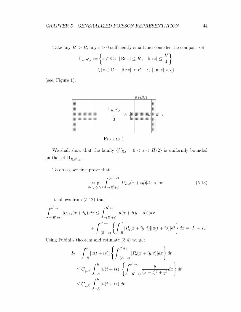
Take any R′> R, any ε > 0 sufficiently small and consider the compact set
ΠR,R′,ε :=
z ∈ C : |Re z| ≤ R
′, | Im z| ≤ H
4
\z ∈ C : |Re z| > R− ε, | Im z| < ε
(see, Figure 1).
q0
R R′
ΠR,R′ ,ε
R+iH/4
R′+εR−ε
Figure 1
ppppppppppppppppppppppppppppppppppppppp
ppppppppppppppppppppppppppppppppppppppp
ppppppppppppppppppppppppppppppppppppppp
ppppppppppppppppppppppppppppppppppppppp
ppppppppppppppppppppppppppppppppppppppp
ppppppppppppppppppppppppppppppppppppppp
ppppppppppppppppppppppppppppppppppppppp
pppppppppppppppppppppppppppppppppppppppp p p p p p p p p p p p p p p p p p p p p p p pp p p p p p p p p p p p p p p p p p p p p p p pp p p p p p p p p p p p p p p p p p p p p p p pp p p p p p p p p p p p p p p p p p p p p p p pp p p p p p p p p p p p p p p p p p p p p p p pp p p p p p p p p p p p p p p p p p p p p p p pp p p p p p p p p p p p p p p p p p p p p p p pp p p p p p p p p p p p p p p p p p p p p p p p p p p p p p p p p p p p p p p p p p p p p p p pp p p p p p p p p p p p p p p p p p p p p p p pp p p p p p p p p p p p p p p p p p p p p p p pp p p p p p p p p p p p p p p p p p p p p p p pp p p p p p p p p p p p p p p p p p p p p p p pp p p p p p p p p p p p p p p p p p p p p p p pp p p p p p p p p p p p p p p p p p p p p p p pp p p p p p p p p p p p p p p p p p p p p p p p
We shall show that the family UR,s : 0 < s < H/2 is uniformly bounded
on the set ΠR,R′ ,ε.
To do so, we first prove that
sup0<y<H/2
∫ (R′+ε)
−(R′+ε)
|UR,s(x + iy)|dx < ∞. (5.13)
It follows from (5.12) that∫ R′+ε
−(R′+ε)
|UR,s(x + iy)|dx ≤∫ R
′+ε
−(R′+ε)
|u(x + i(y + s))|dx
+
∫ R′+ε
−(R′+ε)
∫ R
−R
|Pq(x + iy, t)||u(t + is)|dt
dx =: I1 + I2.
Using Fubini’s theorem and estimate (3.4) we get
I2 =
∫ R
−R
|u(t + is)|
∫ R′+ε
−(R′+ε)
|Pq(x + iy, t)|dx
dt
≤ Cq,R′
∫ R
−R
|u(t + is)|
∫ R′+ε
−(R′+ε)
y
(x− t)2 + y2dx
dt
≤ Cq,R′
∫ R
−R
|u(t + is)|dt

CHAPTER 5. GENERALIZED POISSON REPRESENTATION 45
where Cq,R′ does not depend on y and s. Since 0 < s < H/2, it follows from
(2.10) that I2 is bounded by a constant which does not depend on y or s.
For 0 < y < H/2, we have 0 < y+s < H and (2.10) shows that I1 is uniformly
bounded. Hence (5.13) holds.
Since |UR,s| is subharmonic in C\ [(−∞,−R] ∪ [R,∞)], for z ∈ ΠR,R′ ,ε we
obtain the estimate
|UR,s(z)| ≤ 1
πε2
∫ ∫|ξ+iη−z|≤ε
|UR,s(ξ + iη)|dξdη
≤ 1
πε2
∫ H/2
−H/2
∫ R′+ε
−(R′+ε)
|UR,s(ξ + iη)|dξdη.
By the aid of (5.13) this shows that the family UR,s : 0 < s < H/2 is uniformly
bounded on ΠR,R′ ,ε.
Now, let sk be a sequence such that (5.11) holds. By the Compactness
Principle for harmonic functions (see, Theorem P, p.26), we can extract a subse-
quence (which we also denote by sk) such that the sequence UR,sk is uniformly
convergent on any compact subset of the slit strip
Π =
z ∈ C : | Im z| < H
4
\ [(−∞,−R] ∪ [R,∞)] .
Let UR be the limiting function. Clearly, UR is harmonic in Π and satisfies
U(x) = 0, x ∈ (−R,R). With the choice s = sk in (5.12) and taking limit as
k →∞, we obtain
UR(z) = u(z)−∫ R
−R
Pq(z, t)dνR(t) for 0 < Im z <H
4. (5.14)
The right hand side of (5.14) is a harmonic function in C+. Therefore UR can be
extended harmonically to C+. Since UR(x) = 0, x ∈ (−R,R), the function UR
can further be extended harmonically to C\ [(−∞,−R] ∪ [R,∞)] .
Now let us show that for R2 > R1, the restriction of νR2 to [−R1, R1] coincides
with νR1 .
We have
UR2(z)− UR1(z) +
∫R1<|t|≤R2
Pq(z, t)dνR2(t) =
∫ R1
−R1
Pq(z, t)[dνR1(t)− dνR2(t)].
CHAPTER 5. GENERALIZED POISSON REPRESENTATION 46
The left-hand side is a harmonic function in C\ [(−∞,−R1] ∪ [R1,∞)] vanishing
on (−R1, R1). Since
Pq(z, t) =y
π
1
(x− t)2 + y2+ Q(x, y, t), (5.15)
where Q is a harmonic polynomial in x and y vanishing for y = 0 (see, (3.8),
arguments on p.19 and Theorem G), we see that νR2 coincides with νR1 on
(−R1, R1).
5.3 Harmonic functions with growth restric-
tions on two horizontal lines
Proof of Theorem 2.4. Let ν be the σ-finite Borel measure defined in Lemma 2.3
and q = maxn ∈ N ∪ 0 : n < α. Since α ≤ q + 1, it follows from (2.11) that∫ ∞
−∞
d|ν|(t)1 + |t|q+1
< ∞,
and hence by Theorem 3.3 ∫ ∞
−∞Pq(z, t)dν(t).
represents a function harmonic in C+.
Define
U(z) = u(z)−∫ ∞
−∞Pq(z, t)dν(t).
We shall show that U(z) = Im P (z) with some real polynomial P of degree at
most q.
For any R > 0, we write
U(z) =
u(z)−
∫ R
−R
Pq(z, t)dν(t)
−∫|t|>R
Pq(z, t)dν(t) =: I1 + I2.
It is easy to see from Lemma 2.3 that I1 is a harmonic function in the slit plane
C\ [(−∞,−R] ∪ [R,∞)] vanishing on (−R,R). Using (5.15), we see that I2 has
this property, too. Hence U is continuous in C+, if we set U(x) = 0, x ∈ R.

CHAPTER 5. GENERALIZED POISSON REPRESENTATION 47
By an application of the Symmetry Principle, we can extend U to a harmonic
function in C (which we also denote by U).
Repeating steps 1-3 of the proof of Theorem 5.1, we obtain
|U(reiθ)| ≤ exp(o(r)), r =rk
2→∞. (5.16)
Suppose that we have shown
|U(z)| = O(|z|q+3), z →∞, | Im z| < H
2. (5.17)
Then using the methods of steps 5 and 6 in the proof of Theorem 5.1, we get that
U = ImP (z), where P is a real polynomial of degree at most q + 4. Noting
that the convergence of the first integral in (2.11) implies∫ ∞
−∞
|U(x + iH)|1 + |x|q+1
dx < ∞, (5.18)
we obtain that in fact degree of P is not greater than q and hence the assertion
of Theorem 2.4 holds. Now it only remains to establish (5.17).
Set
v(z) = U(z)−∫ ∞
−∞Pq(x + i(H − y), t)U(t + iH)dt, z = x + iy, y < H. (5.19)
By (5.18) and Theorem 3.3, v is harmonic in z ∈ C : Im z < H and continuous
in z ∈ C : Im z ≤ H, if we set v(x+ iH) = 0, x ∈ R. Hence v can be extended
to a harmonic function in C (which we also denote by v).
Now, we show that there exists a sequence Rk, Rk →∞ such that
|v(reiθ)| ≤ exp(o(r)), r = Rk →∞. (5.20)
Set v(ζ) := v(ζ + iH). Then, by (5.19), with ρk = rk/2−H,∫ 0
−π
|v(ρkeiθ)|| sin θ|dθ ≤
∫ 0
−π
|U(ρkeiθ + iH)|| sin θ|dθ
+
∫ 0
−π
∫ ∞
−∞|Pq(ρke
−iθ, t)||U(t + iH)|dt
| sin θ|dθ
=:I1 + I2.

CHAPTER 5. GENERALIZED POISSON REPRESENTATION 48
From (5.16), we obtain I1 ≤ exp(o(ρk)), ρk → ∞. Using Fubini’s Theorem and
the estimate (3.4), we get I2 ≤ exp(o(ρk)), ρk → ∞ by an argument similar to
that at the end of the first step in the proof of Theorem 5.1. By symmetry,∫ π
0
|v(ρkeiθ)| sin θdθ ≤ exp(o(ρk)), ρk →∞. (5.21)
In the same fashion as in the third step of the proof of Theorem 5.1, we obtain
from (5.21) that
|v(z)| ≤ exp(o(|z|)), |z| = ρk
2→∞.
Since |v| is a subharmonic function in C, (5.20) holds for Rk = ρk/2−H.
Now, we show that
|v(x)| ≤ O(|x|q+2), x →∞, x ∈ R. (5.22)
Since U(x) = 0, x ∈ R, it follows from (5.19) and estimate (3.4) that for |x|sufficiently large
|v(x)| ≤∫ ∞
−∞|Pq(x + iH, t)||U(t + iH)|dt
≤ Dq|x|q∫ ∞
−∞
H
(x− t)2 + H2· 1
(1 + |t|)q−1|U(t + iH)|dt
≤ Dq,H |x|q∫
|t|<1
|U(t + iH)|dt +
∫|t|≥1
|U(t + iH)|1 + |t|q+1
· 2t2
(x− t)2 + H2dt
= O(|x|q) + Dq|x|q max
|t|≥1
2t2
(x− t)2 + H2
∫|t|≥1
|U(t + iH)|1 + |t|q+1
dt
= O(|x|q+2), |x| → ∞.
Therefore, (5.22) is true.
Now, let V be an entire function such that Re V (z) = v(z). Define
F (z) :=
eV (z)−Azq+2
if q is even,
eV (z)−Azq+3if q is odd,
(5.23)
where A > 0 is a constant. It is evident from (5.22) that F is bounded on the
boundary of the strip S := z ∈ C : 0 < Im z < H for a large enough A.
From (5.20), it follows that
|F (z)| ≤ exp exp(o(|z|)), |z| = Rk →∞, z ∈ S.

CHAPTER 5. GENERALIZED POISSON REPRESENTATION 49
Applying Phragmen-Lindelof principle for strip (see, e.g. [19, p.40]), we conclude
that F is bounded on S. From this it follows that
v(z) = log |F (z)|+ O(|z|q+3) ≤ O(|z|q+3), z →∞, z ∈ S. (5.24)
Similarly, replacing V by −V in (5.23), we get
−v(z) ≤ O(|z|q+3), z →∞, z ∈ S. (5.25)
From (5.24) and (5.25) we conclude
|v(z)| = O(|z|q+3), z →∞, z ∈ S. (5.26)
As in proof of (5.22), we show that∣∣∣∣∫ ∞
−∞Pq(x + i(H − y), t)U(t + iH)dt
∣∣∣∣ = O(|z|q+2), z →∞, 0 < Im z < H/2.
(5.27)
Now (5.17) follows from (5.19), (5.26) and (5.27).
5.4 Main result on representation of harmonic
functions by generalized Poisson integrals
Proof of Theorem 2.1. To prove Theorem 2.1, let us note that it suffices to show
that its conditions imply condition (4.13). Then assertion of Theorem 2.1 will
follow from Theorem 5.1.
By condition (2.6) of Theorem 2.1, there exists a constant C > 0 and a
decreasing sequence sl∞l=1 ⊂ (0, 1], liml→∞ sl = 0, such that∫ ∞
−∞
|u(x + isl)|1 + |x|α
dx ≤ C, l = 1, 2, · · · , (5.28)
holds. Clearly, it suffices to show that
supsl<y<s1
∫ ∞
−∞
|u(x + iy)|1 + |x|α
≤ D, l = 1, 2, · · · , (5.29)

CHAPTER 5. GENERALIZED POISSON REPRESENTATION 50
where D does not depend on l.
We want to apply Lemma 3.4 to vl(z) = u(z + isl) for h = hl := s1−sl, l > 1.
It is clear from (5.28) that vl+1 satisfies (3.10) of Lemma 3.4. To show that (3.9)
of Lemma 3.4 is also satisfied, we need to apply Corollary 2.5 of Theorem 2.4
to the function vl+1(z) = u(z + isl+1). It is easy to see that condition (2.12)
is satisfied with H = hl+1. Now, we need to show that there exists a sequence
Rk, Rk →∞ such that∫ π
0
v+l+1(re
iθ) sin θdθ ≤ exp(o(r)), r = Rk →∞.
Let
QR,sl+1= z ∈ C : |z + isl+1| < R ∩ C+, R > sl+1.
Since the function v+l+1(z) is subharmonic in the closure of QR,sl+1
, we have
v+l+1(z) ≤ 1
2π
∫∂QR,sl+1
v+l+1(ζ)
∂GQR,sl+1
∂n(ζ, z)|dζ|, z ∈ QR,sl+1
,
where GQR,sl+1(ζ, z) is the Green function of QR,sl+1
and ∂/∂n is derivative in the
direction of the inner normal.
Let
KR,sl+1= z ∈ C : |z + isl+1| < R, Im z > −sl+1.
According to the Principle of Extension of Domains (see, [4, p.3], or in an equiv-
alent form [22, Ch. IV §2]), we have
∂GQR,sl+1
∂n(ζ, z) ≤
∂GKR,sl+1
∂n(ζ, z), for ζ ∈ ∂QR,sl+1
∩ ∂KR,sl+1, z ∈ QR,sl+1
.
Using the well-known explicit expression for the Green function of a half-disc, we
CHAPTER 5. GENERALIZED POISSON REPRESENTATION 51
get (zsl+1= z + isl+1, ϕsl+1
= arg zsl+1)∫
∂QR,sl+1∩∂KR,sl+1
v+l+1(ζ)
∂GQR,sl+1
∂n(ζ, z)|dζ|
≤∫
∂QR,sl+1∩∂KR,sl+1
v+l+1(ζ)
∂GKR,sl+1
∂n(ζ, z)|dζ|
=
∫ π−arcsin(sl+1/R)
arcsin(sl+1/R)
u+(Reiθ)4R|zsl+1
|(R2 − |zsl+1|2) sin θ sin ϕsl+1
dθ
|Reiθ − zsl+1|2|Re−iθ − zsl+1
|2
≤4(R + |z|+ sl+1)3
(R− |z| − sl+1)3
∫ π
0
u+(Reiθ) sin θdθ. (5.30)
Further, since QR,sl+1⊂ C+, we have
∂GQR,sl+1
∂n(ζ, z) ≤
∂GC+
∂n(ζ, z), for ζ ∈ ∂QR,sl+1
\C+, z ∈ QR,sl+1.
Hence∫∂QR,sl+1
\C+
v+l+1(ζ)
∂GQR,sl+1
∂n(ζ, z)|dζ|
≤∫
∂QR,sl+1\C+
v+l+1(ζ)
∂GC+
∂n(ζ, z)|dζ|
=
∫ √R2−s2l+1
−√
R2−s2l+1
u+(t + isl+1)2y
(x− t)2 + y2dt
≤∫ R
−R
u+(t + isl+1)2ydt
(x− t)2 + y2, z = x + iy ∈ QR,sl+1
. (5.31)
Joining (5.30) and (5.31), we obtain
v+l+1(re
iϕ) ≤ 2(R + r + sl+1)3
π(R− r − sl+1)3
∫ π
0
u+(Reiθ) sin θdθ
+1
π
∫ R
−R
u+(t + isl+1)r sin ϕdt
r2 + t2 − 2rt cos ϕ, reiϕ ∈ QR,sl+1
. (5.32)
For 0 < r < R−sl+1, we have reiϕ ∈ QR,sl+1when 0 < ϕ < π. Let us multiply
both sides of (5.32) by sin ϕ and integrate with respect to ϕ from 0 to π. Using

CHAPTER 5. GENERALIZED POISSON REPRESENTATION 52
the relation (4.12), we obtain∫ π
0
v+l+1(re
iϕ) sin ϕdϕ ≤ 4(R + r + sl+1)3
π(R− r − sl+1)3
∫ π
0
u+(Reiθ) sin θdθ
+ Cq(1 + R)α−2r
∫ ∞
−∞
u+(t + isl+1)dt
1 + |t|α. (5.33)
Remind that function u satisfies (2.5). Set R = rk, r = rk/2−sl+1 in (5.33) where
rk is the sequence from (2.5). Then we see that condition (2.5) is satisfied for
v+l+1(z) with Rk = rk/2− sl+1 instead of rk.
Now, by Corollary 2.5, vl+1 admits the representation
vl+1(z) =
∫ ∞
−∞Pq(z, t)u(t + isl+1)dt + ImPl+1(z), (5.34)
where q = maxn ∈ N ∪ 0, n < α and Pl+1 is a polynomial of degree at most
q. Using representation (5.34) and estimate (3.4), we get
|vl(x + iy)| = |vl+1(x + iy + i(sl − sl+1))|
≤ Cq(1 + |x|+ hl+1)q
∫ ∞
−∞
|u(t + isl+1)|(1 + |t|)q−1
· (y + (sl − sl+1))dt
(x− t)2 + (y + (sl − sl+1))2
+ O(|x|q), |x| → ∞, 0 < y < hl.
As in proof of (5.22), this shows that
|vl(x + iy)| = O(|x|q+2), |x| → ∞, 0 < y < hl,
and hence vl+1 satisfies condition (3.9) of Lemma 3.4. Applying Lemma 3.4, we
get for vl(z) the formula (3.11). Dividing both its sides by 1 + |x|α, integrating
with respect to x and changing the order of integration, we obtain∫ ∞
−∞
|u(x + i(sl + y))|1 + |x|α
dx ≤∫ ∞
−∞|u(t + isl)| · I+
l (t)dt
+
∫ ∞
−∞|u(t + is1)| · I−l (t)dt, 0 < y < hl. (5.35)
where
I±l (t) =sin(πy/hl)
2hl
∫ ∞
−∞
dx
(cosh[π(x− t)/hl]± cos(πy/hl))(1 + |x|α).

CHAPTER 5. GENERALIZED POISSON REPRESENTATION 53
Let us estimate I±l (t):
I±l (t) =sin(πy/hl)
2hl
∫|x|>|t|/2
+sin(πy/hl)
2hl
∫|x|<|t|/2
=: I±1,l(t) + I±2,l(t).
Evidently,
I±1,l(t) ≤1
1 + |t/2|α· sin(πy/hl)
2hl
∫ ∞
−∞
dx
cosh[π(x− t)/hl]± cos(πy/hl);
I±2,l(t) ≤1
2hl
∫|x|<|t|/2
dx
cosh[π(x− t)/hl]− 1≤ 1
2hl
|t|/2cosh(πt/(2hl))− 1
.
Choosing n ∈ N in such a way that 2n > α+1 and using the inequality cosh τ−1 ≥τ 2n/(2n)!, we get
I±2,l(t) ≤|t|4hl
· (2n)!(2hl)2n
(π|t|)2n≤ D1
1 + |t|α, for |t| ≥ 1, (5.36)
where D1 does not depend on l (remind that hl < 1).
Note that by Lemma 3.4 for v(z) ≡ 1, we have the identity
1 =sin(πy/hl)
2hl
∫ ∞
−∞
dx
cosh[π(x− t)/hl]− cos(πy/hl)
+
∫ ∞
−∞
dx
cosh[π(x− t)/hl] + cos(πy/hl)
,
and both integrals in the right hand side are positive. Hence we conclude that
I±1,l(t) ≤D2
1 + |t|α, t ∈ R,
and, moreover,
I±l (t) = I±1,l(t) + I±2,l(t) ≤ 1, t ∈ R.
Using this and (5.36), we conclude that
I±l (t) ≤ D3
1 + |t|α, t ∈ R,
where D3 does not depend on l and t.
Substituting this estimate into (5.35), we obtain∫ ∞
−∞
|u(x + isl + iy)|1 + |x|α
dx ≤ D3
∫ ∞
−∞
|u(t + isl)|+ |u(t + is1)|1 + |t|α
dt
≤ 2D3C, 0 < y < s1 − sl,
where C is the constant from (5.28), and (5.29) follows.
Chapter 6
Applications to the Hardy and
the Nevanlinna classes
6.1 Factorization in the Nevanlinna class
Proof of Theorem 2.6. Since h belongs to the Nevanlinna class its zeros satisfy
the Blaschke condition (see, Corollary 3.5, p.24). Therefore the zeros of g1 and
g2 also satisfy this condition.
Denote by B1 the Blaschke product corresponding to the zeros of g1. The
function
f :=g1
B1
is analytic and non-vanishing in C+. So log |f | is harmonic in C+.
Let us show that log |f | satisfies the conditions of Corollary 2.2.
We have∫ π
0
log+ |f(reiθ)| sin θdθ ≤∫ π
0
log+ |g1(reiθ)| sin θdθ
+
∫ π
0
log+ 1
|B1(reiθ)|sin θdθ.
54

CHAPTER 6. APPL. TO THE HARDY AND NEVANLINNA CLASSES 55
Thus, it follows from (2.14) and Lemma 4.1 that log |f | satisfies condition (2.7)
of Corollary 2.2.
Observe also that∫ ∞
−∞
| log |f(t + is)||1 + t2
dt ≤∫ ∞
−∞
| log |g1(t + is)||1 + t2
dt +
∫ ∞
−∞
log+ |1/B1(t + is)|1 + t2
dt.
Further∫ ∞
−∞
| log |g1(t + is)||1 + t2
dt =
∫ ∞
−∞
log+ |g1(t + is)|1 + t2
dt +
∫ ∞
−∞
log+ |1/g1(t + is)|1 + t2
dt,
and∫ ∞
−∞
log+ |1/g1(t + is)|1 + t2
dt =
∫ ∞
−∞
log+ |g2(t + is)/h(t + is)|1 + t2
dt
≤∫ ∞
−∞
log+ |g2(t + is)|1 + t2
dt +
∫ ∞
−∞
log+ |1/h(t + is)|1 + t2
dt.
So, combining all these together, we get∫ ∞
−∞
| log |f(t + is)||1 + t2
dt ≤∫ ∞
−∞
log+ |g1(t + is)|1 + t2
dt +
∫ ∞
−∞
log+ |g2(t + is)|1 + t2
dt
+
∫ ∞
−∞
log+ |1/h(t + is)|1 + t2
dt +
∫ ∞
−∞
log+ |1/B1(t + is)|1 + t2
dt.
Now, by condition (2.15) and Corollary 3.6 (see, p.25) we see that log |f | also
satisfies condition (2.8) of Corollary 2.2.
Applying Corollary 2.2 to the function log |f |, we get the following represen-
tation:
log |f(z)| = y
π
∫ ∞
−∞
dν(t)
(x− t)2 + y2+ cy, z = x + iy ∈ C+,
where ν is a real-valued Borel measure satisfying∫ ∞
−∞
d|ν|(t)1 + t2
< ∞,
and c is a real constant.
Let us complete the proof of the theorem.
CHAPTER 6. APPL. TO THE HARDY AND NEVANLINNA CLASSES 56
Taking into account that |g1| ≤ |f | for z ∈ C+, we obtain
log |g1| ≤ log |f | ≤ y
π
∫ ∞
−∞
dν+(t)
(x− t)2 + y2+ c+y
where c+ = max(c, 0).
Thus log |g1| has positive harmonic majorant, that is, g1 belongs to the Nevan-
linna class.
Since h and g1 are functions of the Nevanlinna class, by Theorem J (see, p.24)
and its Corollary 3.5, we can write h and g1 in the form
h = B · H1
H2
g1 = B1G1
G2
where B and B1 are Blaschke products formed by zeros of h and g1 respectively,
Hj, Gj are analytic and non-vanishing in C+ such that |Hj| < 1, |Gj| < 1. Then
g2 is in the form
g2 =h
g1
=B
B1
· H1G2
H2G1
.
Note that B2 := B/B1 is the Blaschke product formed by zeros of g2 and
therefore B2 is analytic in C+ and |B2| < 1. Putting F1 := B2H1G2 and F2 :=
H2G1, we write g2 = F1/F2 where Fj’s are analytic in C+ and |Fj| < 1, j = 1, 2,
and F2 6= 0. Hence, by Theorem J (see, p.24) g2 belongs to the Nevanlinna
class.
Proof of Corollary 2.7. Clearly h, g1 and g2 satisfy the conditions of Theorem 2.6.
Then according to the Theorem 2.6, g1 and g2 belong to the Nevanlinna class.
Thus Corollary 2.7 follows from Lemma 4.4.
Now let us consider some examples related to the sharpness of Theorem 2.6.
Example 6.1. Consider the functions g1(z) = exp(cos z), g2(z) = exp(− cos z).
Evidently, these functions satisfy condition (2.14) with “O(r)” instead of “o(r)”,
satisfy condition (2.15) and satisfy g1g2 ≡ 1 ∈ H∞(C+). Nevertheless, neither g1
nor g2 belongs to the Nevanlinna class. Indeed, if f is a function belonging to

CHAPTER 6. APPL. TO THE HARDY AND NEVANLINNA CLASSES 57
the Nevanlinna class, then by representation (4.27) and similar estimation as in
the proof of Lemma 4.4 (cf. (4.28)), we have
log+ |f(z)| ≤ ky + o(|z|), |z| → ∞, |π/2− arg z| ≤ π/4. (6.1)
But, in our case log+ |g1(iy)| = (ey + e−y)/2 does not satisfy the above in-
equality. This shows that g1 does not belong to the Nevanlinna class. Hence g2
does not belong to the Nevanlinna class. This example shows that the condition
(2.14) cannot be weakened replacing o(r) by O(r).
The following example shows that the condition (2.15) in Theorem 2.1 cannot
be weakened by replacing it with
∃H > 0, sup0<s<H
∫ ∞
−∞
log+ |gj(t + is)|1 + |t|α
dt < ∞, j = 1, 2,
for some α > 2.
Example 6.2. Consider the functions g1(z) = expiz2, g2(z) = exp−iz2.Since log |g1(t+is)| = −2ts, log |g2(t+is)| = 2ts, they satisfy the above condition.
The condition (2.14) of Theorem 2.1 and g1g2 ≡ 1 ∈ H∞(C+) are also satisfied.
Nevertheless, neither g1 nor g2 belongs to the Nevanlinna class by the same reason
as in the Example 6.1, now it is enough to look the growth of log+ |g1| and log+ |g2|on the rays z ∈ C : arg z = 3π/4 and z ∈ C : arg z = π/4 respectively.
The condition (2.14) of Theorem 2.1 touches only one of the functions g1, g2.
But it is impossible to change the condition (2.15) in a similar way as the following
example shows.
Example 6.3. Consider the functions g1(z) = expz2, g2(z) = exp−z2.Clearly g1 and g2 satisfy the condition (2.14) and satisfy g1g2 ≡ 1 ∈ H∞(C+) and
g2 satisfy condition (2.15) but for any ε > 0
sup0<s<ε
∫ ∞
∞
log+ |g1(t + is)|1 + t2
dt = ∞.
In this case, we see by the same reason as in the previous examples that neither
g1 nor g2 belong to the Nevanlinna class.
CHAPTER 6. APPL. TO THE HARDY AND NEVANLINNA CLASSES 58
6.2 Factorization in H∞(C+) when the factors
are connected by a linear equation
Proof of Theorem 2.8. We divide the proof into 4 steps.
1. Let us show that
log+ |gj(reiϕ)| ≤ Cr
sin ϕlog
Cr
sin ϕ, reiϕ ∈ C+, r ≥ 1, j = 1, · · · , n, (6.2)
where C is a positive constant.
Map C+ onto D = ζ ∈ C : |ζ| < 1 by
ζ =z − i
z + i(6.3)
and set
h(ζ) = h(z), gj(ζ) = gj(z), j = 1, · · · , n.
Then
h(ζ) = g1(ζ) · · · gn(ζ), (6.4)
gn(ζ) = g1(ζ) + · · ·+ gn−1(ζ).
Moreover, h is bounded in D and g1, · · · gn−1 are linearly independent over C.
Since the zeros of h satisfy the Blaschke condition for the upper half-plane, the
zeros of h satisfy the Blaschke condition for the unit disk, equation (6.4) implies
that the zeros of g1, · · · gn−1 also satisfy this condition. Applying Theorem R (see,
p.28), we get
T (r, gj/gn) = O
(log
1
1− r
), r → 1, j = 1, · · · , n− 1. (6.5)
Using the properties of the Nevanlinna characteristic (see, p.27) and taking
into account that boundedness of h in D implies T (r, h) = O(1), r → 1, we
obtain
T (r, gn) = T
(r,
1
gn
)+ O(1) =
1
nT
(r,
1
(gn)n
)+ O(1)
≤ 1
nT
(r,
h
(gn)n
)+
1
nT (r, h) + O(1) =
1
nT
(r,
h
(gn)n
)+ O(1), r → 1,

CHAPTER 6. APPL. TO THE HARDY AND NEVANLINNA CLASSES 59
whence, using (6.4) and (6.5), we conclude
T (r, gn) ≤ 1
nT
(r,
g1 · · · gn
(gn)n
)+ O(1)
≤ 1
n
n−1∑j=1
T
(r,
gj
gn
)+ O(1) = O
(log
1
1− r
), r → 1.
Using (6.5) once again, we get
T (r, gj) ≤ T
(r,
gj
gn
)+ T (r, gn) + O(1) = O
(log
1
1− r
), r → 1, j = 1, · · · , n.
(6.6)
The inequality
log+ M(r, gj) ≤4
1− rT
(1 + r
2, gj
)allows us to derive from (6.6) that there is a positive constant C1, such that
log+ |gj(ζ)| ≤ C1
1− |ζ|log
C1
1− |ζ|, ζ ∈ D, j = 1, · · · , n.
Since (6.3) implies
1− |ζ| ≥ 1
2(1− |ζ|2) =
1
2
|z + i|2 − |z − i|2
|z + i|2=
2 Im z
|z + i|2≥ Im z
2|z|2, |z| ≥ 1,
and gj(ζ) = gj(z), we get (6.2).
2. Let us show that
sup
∫ ∞
−∞
| log |gj(x + iy)||1 + x2
dx : 0 < y < H
< ∞, j = 1, · · · , n, (6.7)
where H is taken from the condition (2.16) of Theorem 2.8.
To prove (6.7), note that∫ ∞
−∞
| log |gj(x + iy)||1 + x2
dx =
∫ ∞
−∞
log+ |gj(x + iy)|1 + x2
dx
+
∫ ∞
−∞
log+ |1/gj(x + iy)|1 + x2
dx. (6.8)

CHAPTER 6. APPL. TO THE HARDY AND NEVANLINNA CLASSES 60
The first integral in the right hand side is bounded for 0 < y < H by the condition
(2.16) of Theorem 2.8. Using condition (2.16) once again, we get
1
|gj(x + iy)|=
1
|h(x + iy)|∏k 6=j
|gk(x + iy)| ≤ C
|h(x + iy)|, 0 < y < H,
where C is a positive constant. Hence, the boundedness of the second integral
in the right hand side of (6.8) is a consequence of Theorem L with Q = h (see,
p.25).
3. Denote by Bj the Blaschke product formed by the zeros of gj and set
uj := log
∣∣∣∣ gj
Bj
∣∣∣∣ , j = 1, · · · , n.
This is a harmonic function in C+. Let us show that it satisfies conditions of
Corollary 2.2.
We have∫ π
0
u+j (reiϕ) sin ϕdϕ ≤
∫ π
0
log+ |gj(reiϕ)| sin ϕdϕ
+
∫ π
0
log+ 1
|Bj(reiϕ)|sin ϕdϕ. (6.9)
The estimate (6.2) implies that the first integral in the right hand side is O(r log r)
as r →∞. Applying Lemma 4.1 to Bj(z), we get that the second integral in (6.9)
is O(r) as r →∞. Hence, uj satisfies the condition (2.7) of Corollary 2.2.
Further we have∫ ∞
−∞
|uj(x + iy)|1 + x2
dx ≤∫ ∞
−∞
| log |gj(x + iy)||1 + x2
dx +
∫ ∞
−∞
log+ |1/Bj(x + iy)|1 + x2
dx.
Using (6.7) for the first integral in the right hand side and Theorem L for the
second one, we see that condition (2.8) of Corollary 2.2 is also satisfied.
4. Let us complete the proof of Theorem 2.8.
Applying Corollary 2.2, we get the representation
uj(z) =y
π
∫ ∞
−∞
dνj(t)
(t− x)2 + y2+ kjy, z = x + iy ∈ C+,
CHAPTER 6. APPL. TO THE HARDY AND NEVANLINNA CLASSES 61
where kj is a real constant, νj is a real-valued Borel measure such that∫ ∞
−∞
d|νj|(t)1 + t2
< ∞.
Thus,
log |gj(z)| = log |Bj(z)|+ y
π
∫ ∞
−∞
dνj(t)
(t− x)2 + y2+ kjy, z = x + iy ∈ C+,
and hence, gj belongs to the Nevanlinna class. Using Lemma 4.4, we conclude
that gj(z)eiαjz ∈ C+ for some real number αj.
6.3 A criterion of belonging to Hp(C+) up to an
exponential factor
Proof of Theorem 2.9.
Case I. Firstly, we prove the theorem under additional assumption that f is
analytic in the closed half-plane C+ and does not vanish on R.
Let B be the Blaschke product formed by the zeros of f . Set
g :=f
B, u := log |g|. (6.10)
The function g is analytic and non-vanishing in the closed half-plane C+ and
therefore u is harmonic in C+. We will show that u satisfies the conditions of
Corollary 2.5 with α = 2.
We have∫ π
0
u+(reiϕ) sin ϕdϕ ≤∫ π
0
log+ |f(reiϕ)| sin ϕdϕ +
∫ π
0
log+ 1
|B(reiϕ)|sin ϕdϕ.
The second integral in the right hand side is O(r), as r → ∞ (see, Lemma 4.1,
p.30). Therefore condition (2.5) follows from (2.18).
Further,∫ ∞
−∞
|u(x + iy)|1 + x2
dx ≤∫ ∞
−∞
| log |f(x + iy)||1 + x2
dx +
∫ ∞
−∞
log+ |1/B(x + iy)|1 + x2
dx.
CHAPTER 6. APPL. TO THE HARDY AND NEVANLINNA CLASSES 62
The second integral in the right hand side is bounded on any finite interval of
values of y > 0 (see, Theorem L, p.25). For the first integral, we have∫ ∞
−∞
| log |f(x + iy)||1 + x2
dx =
∫ ∞
−∞
log+ |f(x + iy)|1 + x2
dx +
∫ ∞
−∞
log− |f(x + iy)|1 + x2
dx
≤ Cp
∫ ∞
−∞|f(x + iy)|pdx +
∫ ∞
−∞
log− |f(x + iy)|1 + x2
dx.
Therefore, the condition (2.12) follows from (2.19) and (2.20).
So, Corollary 2.5 is applicable to function u defined by (6.10), and hence the
representation (2.9) holds with ν(t) = log |g(t)|dt.
Since |B(t)| = 1 for t ∈ R, we have
|g(t)| = |f(t)|, dν(t) = log |f(t)|dt.
Hence, the representation (2.9) can be rewritten in the form
log |g(z)| = y
π
∫ ∞
−∞
log |f(t)|(t− x)2 + y2
dt + ky, z = x + iy ∈ C+.
Taking into account that |f(z)| ≤ |g(z)|, z ∈ C+, we obtain
log |f(z)| ≤ y
π
∫ ∞
−∞
log |f(t)|(x− t)2 + y2
dt + ky.
It follows from the above representation and arithmetic-geometric mean inequal-
ity (see, e.g. [7, p.29]) that
|f(z)eikz|p ≤ exp
y
π
∫ ∞
−∞
log(|f(t)|p)(x− t)2 + y2
dt
≤ y
π
∫ ∞
−∞
|f(t)|p
(x− t)2 + y2dt, z = x + iy ∈ C+.
By Fubini’s theorem, we have∫ ∞
−∞|f(x + iy)eik(x+iy)|pdx ≤
∫ ∞
−∞|f(t)|p
y
π
∫ ∞
−∞
1
(x− t)2 + y2dx
dt
=
∫ ∞
−∞|f(t)|pdt,
and hence f(z)eikz ∈ Hp(C+).

CHAPTER 6. APPL. TO THE HARDY AND NEVANLINNA CLASSES 63
Case II. Now, let f be any function satisfying conditions (2.17)-(2.20).
Let s ∈ (0, H) be such that f(t + is) 6= 0 for t ∈ R. Set
fs(z) := f(z + is).
This function is analytic in the closed half-plane C+ and does not vanish on R.
It suffices to show that
‖f(·+ iy)eik(·+iy)‖p (6.11)
is bounded for s ≤ y < ∞ (for some k ∈ R). Boundedness of (6.11) for 0 < y < s
follows from (2.20) because s < H.
In order to apply the result of part I of the proof, we should check that
conditions (2.17), (2.18), (2.19), (2.20) are satisfied for fs(z). It is trivial that
(2.19) and (2.20) are satisfied with H − s instead of H because 0 < s < H.
To check (2.17), note that, if zk is a zero of f , then zk − is is a zero of fs.
Therefore,∑Im zk>s
Im(zk − is)
1 + |zk − is|2≤(
maxIm zk>s
1 + |zk|2
1 + |zk − is|2
) ∑Im zk>s
Im zk
1 + |zk|2< ∞.
It remains to check (2.18).
Let
QR,s := z ∈ C : |z + is| < R ∩ C+, R > s.
Note that the function log+ |fs(z)| is subharmonic in the closure of QR,s.
Therefore, using the arguments in pages 51-51, we obtain
log+ |fs(reiϕ)| ≤ 2(R + r + s)3
π(R− r − s)3
∫ π
0
log+ |f(Reiθ)| sin θdθ
+1
π
∫ ∞
−∞log+ |f(t + is)| r sin ϕdt
r2 + t2 − 2rt cos ϕ, reiϕ ∈ QR,s. (6.12)
For 0 < r < R − s, we have reiϕ ∈ QR,s for 0 < ϕ < π. Let us multiply both
sides of (6.12) by sin ϕ and integrate with respect to ϕ from 0 to π. Using the

CHAPTER 6. APPL. TO THE HARDY AND NEVANLINNA CLASSES 64
relation (4.12), we obtain∫ π
0
log+ |fs(reiϕ)| sin ϕdϕ ≤ 4(R + r + s)3
π(R− r − s)3
∫ π
0
log+ |f(Reiθ)| sin θdθ
+ r
∫ ∞
−∞log+ |f(t + is)| dt
1 + t2. (6.13)
Let rk be the sequence staying in (2.18). Put R = rk, r = rk/2 − s in (6.13).
Then we see that condition (2.18) is satisfied for fs with rk/2 − s instead of
rk.
Now, let us consider examples showing that conditions (2.17), (2.18), (2.19),
(2.20) are independent, and moreover, (2.18) and (2.20) cannot be substantially
weakened.
Example 6.4. Let
Eρ(z) =∞∑
k=0
zk
Γ(1 + k/ρ), ρ > 1,
be Mittag-Leffler’s entire function. It is known (see, e.g., [3, p.275]) that the
following asymptotic formula holds as z →∞ :
Eρ(z) =
− 1
zΓ(1−1/ρ)+ O( 1
|z|2 ),π2ρ≤ arg z ≤ 2π − π
2ρ,
ρezρ+ O( 1
|z|), − π2ρ≤ arg z ≤ π
2ρ.
This implies that the function
f(z) = (z + i)−2/pEρ(−iz)
satisfies (2.18), (2.19), (2.20).
Since each Hp(C+) is a subclass of the Nevanlinna class, it follows from The-
orem K, p.24 that if a function belongs to Hp(C+) up to factor eikz, k ∈ R, it
should belong to the Nevanlinna class.
Therefore, f does not belong to Hp(C+) up to an exponential factor because
f(iy) = ρ(y + 1)−2/peyρ
(1 + o(1)), y →∞,
and this contradicts to the fact that any function belonging to the Nevanlinna
class should satisfy the estimate (6.1).

CHAPTER 6. APPL. TO THE HARDY AND NEVANLINNA CLASSES 65
Example 6.5. The function
f(z) = e−z2
satisfies (2.17), (2.18), (2.20). But it does not belong to Hp(C+) up to an expo-
nential factor (see, Example 6.3). Here (2.19) is violated.
Example 6.6. The function
f(z) = (z + i)−2/pe−iz3
satisfies (2.17), (2.18), (2.19), but f does not belong to Hp(C+) up to an expo-
nential factor. Here (2.20) is violated. This example also shows that Theorem
2.9 ceases to be true if (2.20) is replaced with ‖f(·+ i0)‖p < ∞.
Example 6.7. The function
f(z) = (z + i)−2/p exp exp(−ciz), c > 0,
satisfies (2.17), (2.19), (2.20), but evidently it does not belong to Hp(C+) up to
an exponential factor (e.g., f does not satisfy (6.1)). Here (2.18) is violated.This
example also shows that Theorem 2.9 ceases to be true if “O” is replaced with
“o” in (2.18).

Chapter 7
Application to generalization of
the Titchmarsh convolution
theorem
Proof of Theorem 2.10. If `(µj) > −∞, j = 1, · · · , n, then (2.26) follows from
the Titchmarsh theorem (see, Theorem S, p.29). If `(µ1 ∗ · · · ∗ µn) = −∞, then
(2.26) follows from the inequality (3.16). Hence, Theorem 2.10 will be proved if
we prove the following fact.
Theorem 7.1 Under the hypotheses of Theorem 2.10, the following implication
holds:
`(µ1 ∗ µ2 ∗ · · · ∗ µn) > −∞⇒ `(µj) > −∞, j = 1, . . . , n.
Proof. Let µ := µ1 ∗ µ2 ∗ · · · ∗ µn. Without loss of generality we can assume that
`(µ1 ∗ µ2 ∗ · · · ∗ µn) = 0. Thus, the Fourier transform µ of the measure µ satisfies
|µ(z)| =∣∣∣∣∫ ∞
0
eitzdµ(t)
∣∣∣∣ ≤ ∫ ∞
0
e−ytd|µ|(t) ≤ |µ|((0,∞)), z = x + iy ∈ C+.
Therefore µ belongs to H∞(C+) and continuous on C+.
66

CHAPTER 7. APPL. TO TITCHMARSH CONVOLUTION THEOREM 67
For z ∈ C+ we have
µj(z) =
∫ ∞
−∞eitzdµj,1(t) +
∫ ∞
−∞eitzdµj,2(t)
=: µj,1(z) + µj,2(z),
where µj,1 and µj,2 are the restrictions of µj to R− and R+, respectively. Similar
to µ, µj,2 belongs to H∞(C+) and continuous on C+ and µj,1 is bounded analytic
function on C− := z ∈ C : Im z < 0 and continuous on C− := z ∈ C : Im z ≤0. We will show that µj,1 converges absolutely and uniformly on any horizontal
strip of C+ and therefore represents an entire function.
Note that
|µj,1(z)| ≤∫ 0
−∞e−ytd|µj|(t)
= e−yt|µj|((−∞, t))
∣∣∣∣0−∞
+ y
∫ 0
−∞e−yt|µj|((−∞, t))dx.
Fix c > 0. It follows from the condition (2.25) that there exists Nc > 0 and
Ac > 0 such that |µj|((−∞, t)) ≤ Ace−ct, t ≤ −Nc. For 0 ≤ y < c, we have
|µj(z)| ≤ |µj|((−∞, 0)) + cAc
∫ −Nc
−∞e(c−y)tdt + c
∫ 0
−Nc
e−yt|µj|((−∞, 0))dt = Bc.
Thus, µj is a function analytic in C+ and uniformly bounded in each horizontal
strip of C+. For z ∈ R, we have
µ = µ1µ2 · · · µn. (7.1)
Since, µ and µj, j = 1, · · · , n are continuous on C+, the equation (7.1) holds in
C+.
Taking into account that µn = µ1 + · · · + µn−1, we see that Theorem 2.8 is
applicable to h = µ, gj = µj, j = 1, · · · , n. By Theorem 2.8, we obtain that
µj(z) expibjz ∈ H∞(C+), j = 1, · · · , n. Thus,
|µj,1(z)| ≤ C1e|bj ||z|, z ∈ C+.
We have already noted that µj,1 is bounded on C−. Using the well-known corol-
lary of the Paley-Wiener theorem (see, Theorem T, p.29), we get supp µj,1 ⊂

CHAPTER 7. APPL. TO TITCHMARSH CONVOLUTION THEOREM 68
[−|bj|, |bj|] and hence supp µj ⊂ [−|bj|,∞). This proves that `(µj) > −∞,
j = 1, · · · , n.
The following example shows that the condition (2.25) in Theorem 2.10 cannot
be weakened by replacing ‘∀’ by ‘∃’.
Example 7.1. Let µ1, µ2, µ3 be the measures defined by the Fourier transforms
µ1(z) =1
1 + iz/c, µ2(z) =
(1 + iz/c)2
(1− iz/c)4, µ3(z) = µ1(z) + µ2(z).
where c is a positive constant. The direct calculation of the inverse Fourier
transform shows that the condition (2.25) is satisfied with the given fixed c > 0,
and `(µ1) = `(µ2) = `(µ3) = −∞. Nevertheless, the product µ1µ2µ3 belongs to
H2(C+) ∩H∞(C+) and therefore `(µ1 ∗ µ2 ∗ µ3) = 0 (see, [2, p.75]).
Bibliography
[1] L. V. Ahlfors, Complex analysis: An introduction to the theory of analytic
functions of one complex variable, third ed., McGraw-Hill Book Co., New
York, 1978.
[2] N. I. Akhiezer, Lectures on integral transforms, Translations of Mathematical
Monographs, vol. 70, American Mathematical Society, Providence, RI, 1988.
[3] L. Bieberbach, Lehrbuch der Funktionentheorie. I. Elemente der Funktionen-
theorie. II. Moderne Funktionentheorie, Chelsea Publishing Company, New
York, 1945.
[4] T. Carleman, Sur les fonctions inverses des fonctions entieres d’ordre fini,
Ark. Mat. 15 (1921), no. 10, 1–7.
[5] H. Cartan, Sur les zeros des combinaisons lineaires de p fonctions holomor-
phes donnes, Mathematica, Cluji 7 (1933), 5–31.
[6] Y. Domar, Extensions of the Titchmarsh convolution theorem with applica-
tions in the theory of invariant subspaces, Proc. London Math. Soc. (3) 46
(1983), no. 2, 288–300.
[7] P. L. Duren, Theory of Hp spaces, Pure and Applied Mathematics, Vol. 38,
Academic Press, New York, 1970.
[8] S. Gergun and I. V. Ostrovskii, On the Poisson representation of a function
harmonic in the upper half-plane, Mat. Fiz. Anal. Geom. 9 (2002), no. 2,
243–248.
69

BIBLIOGRAPHY 70
[9] , On the Poisson representation of a function harmonic in the upper
half-plane, Comput. Methods Func. Theory 2 (2002), no. 1, 191–213.
[10] , On a criterion of belonging to the Hardy class Hp(C+) up to an
exponential factor, Mat. Fiz. Anal. Geom. (to appear).
[11] S. Gergun, I. V. Ostrovskii, and A. Ulanovskii, On the Titchmarsh convolu-
tion theorem, C. R. Acad. Sci. Paris Ser. I Math. 331 (2000), no. 1, 41–46.
[12] , On the Titchmarsh convolution theorem, Ark. Mat. 40 (2002), no. 1,
55–71.
[13] A. A. Gol′dberg and I. V. Ostrovskiı, Raspredelenie znachenii meromorfnykh
funktsii, Izdat. “Nauka”, Moscow, 1970.
[14] N. V. Govorov, Riemann’s boundary problem with infinite index, Operator
Theory: Advances and Applications, vol. 67, Birkhauser Verlag, Basel, 1994.
[15] K. Hoffman, Banach spaces of analytic functions, Dover Publications Inc.,
New York, 1988.
[16] P. Koosis, Introduction to Hp spaces, second ed., Cambridge Tracts in Math-
ematics, vol. 115, Cambridge University Press, Cambridge, 1998.
[17] , The logarithmic integral. I, Cambridge Studies in Advanced Math-
ematics, vol. 12, Cambridge University Press, Cambridge, 1998.
[18] B. Ya. Levin, Distribution of zeros of entire functions, revised ed., Transla-
tions of Mathematical Monographs, vol. 5, American Mathematical Society,
Providence, R.I., 1980.
[19] , Lectures on entire functions, Translations of Mathematical Mono-
graphs, vol. 150, American Mathematical Society, Providence, RI, 1996.
[20] Ju. V. Linnik and I. V. Ostrovs′kiı, Decomposition of random variables and
vectors, American Mathematical Society, Providence, R. I., 1977.
[21] R. Nevanlinna, Uber die Eigenschaften meromorpher Funktionen in einem
Winkelraum, Acta Soc. Sci. Fenn. 50 (1925), no. 12, 1–45.

BIBLIOGRAPHY 71
[22] , Analytic functions, Springer-Verlag, New York, 1970.
[23] I. V. Ostrovskiı, Generalization of the Titchmarsh convolution theorem and
the complex-valued measures uniquely determined by their restrictions to a
half-line, Stability problems for stochastic models (Uzhgorod, 1984), Lecture
Notes in Math., vol. 1155, Springer, Berlin, 1985, pp. 256–283.
[24] E. C. Titchmarsh, The zeros of certain integral functions, Proc. London
Math. Soc. 25 (1926), 283–302.


