Representation Theory - GitHub Pages Notes/Representation Theory... · Representation theory, at...

Representation Theory

Daniel Raban

Contents

0.1 Note to the reader . . . . . . . . . . . . . . . . . . . . . . . . . . . . 20.2 Motivation . . . . . . . . . . . . . . . . . . . . . . . . . . . . . . . . . 3

1 Representation theory of finite groups over C 41.1 Representations . . . . . . . . . . . . . . . . . . . . . . . . . . . . . . 4

1.1.1 Definition and examples . . . . . . . . . . . . . . . . . . . . . 41.1.2 Change of basis . . . . . . . . . . . . . . . . . . . . . . . . . . 7

1.2 Vector space constructions of representations . . . . . . . . . . . . . . 91.2.1 Direct sum, tensor product and dual representations . . . . . . 91.2.2 Subrepresentations and decomposition into irreducible repre-

sentations . . . . . . . . . . . . . . . . . . . . . . . . . . . . . 101.2.3 Hom(V,W ), HomG(V,W ), and Schur’s lemma . . . . . . . . . 14

1.3 Characters of Representations . . . . . . . . . . . . . . . . . . . . . . 181.3.1 Characters and class functions . . . . . . . . . . . . . . . . . . 181.3.2 Orthogonality of characters . . . . . . . . . . . . . . . . . . . 201.3.3 The regular representation . . . . . . . . . . . . . . . . . . . . 231.3.4 Character tables . . . . . . . . . . . . . . . . . . . . . . . . . 27

A Linear Algebra Background 32A.1 The trace . . . . . . . . . . . . . . . . . . . . . . . . . . . . . . . . . 32A.2 Products and Direct sums . . . . . . . . . . . . . . . . . . . . . . . . 35A.3 Dual spaces . . . . . . . . . . . . . . . . . . . . . . . . . . . . . . . . 37A.4 Tensor products of vector spaces . . . . . . . . . . . . . . . . . . . . . 40

1

CONTENTS 2

0.1 Note to the reader

I’ve always found resources on representation theory to be frustrating to read. Someomit too many details for the level of my background. Some discuss everything interms of modules, a perspective which I don’t really find intuitive at all. But repre-sentation theory is a really nice theory, and I think it should be more accessible tomore people. So here’s my attempt at writing the reprsentation theory introductionI’ve wanted to read,

These notes assume you’ve taken a course in abstract algebra that included grouptheory and that you’ve taken a course in linear algebra which talked about vectorspaces and inner products. Representation theory needs a few fancy linear algebraconcepts, so I’ve included an appendix which explains them. Although it’s calledan “appendix,” I really recommend you read the whole appendix first, as if it wereChapter 0.1

If I’ve written something incorrect or unclear, please don’t hesitate to send mean email letting me know. If you have ideas about how to better organize the notesor even ways I could make them look nicer, please let me know. Thanks for reading!

1Unless you’re some linear algebra deity, skimming the appendix will at least reassure you thatyou know all the relevant information.

CONTENTS 3

0.2 Motivation

Mathematics is often about recognizing structure that was “there all along.” Inthe case of group theory, which can be thought of as the study of the structureof symmetries, there is a natural structure that is often brushed over: “the actionof symmetries on space.” If you consider a group of reflections or rotations, youare probably already imagining some sort of action on space, namely reflections androtations. Representation theory, at the basic level, is about exploring this viewpointof symmetry through the lens of linear algebra.

Why does this viewpoint merit its own theory? Linear algebra has a lot ofstructure and is very nice, compared to theories such as real analysis, which arefilled with counterexamples to intuitive notions. Since group theory can be verymessy, “filtering” information about a group into information in the language oflinear algebra provides an easy to compute but still useful reduction of the theory.Besides, it’s cool!

Chapter 1

Representation theory of finitegroups over C

1.1 Representations

1.1.1 Definition and examples

Example 1.1.1. Consider the dihedral group D8, the group of rotations and reflec-tions of a square. You may already be imagining the square as lying in the planesimilar to this:

4

CHAPTER 1. REPRESENTATION THEORY OF FINITE GROUPS OVER C 5

The group D8 has 8 elements, where e is the identity rotation, s is reflection aboutthe x-axis, and r is counterclockwise rotation by 90 degrees:

D8 = {e, s, r, r2, r3, sr, sr2, sr3}.

Here, we view the element sr as meaning “first rotate, then reflect”; that is, weread the action from right to left. The group has an inherent “multiplication” bycomposing the reflections and rotations, and we can calculate that r4 = e (rotating 4times by 90 degrees does nothing in total) and s2 = e (reflecting twice does nothing).We can also work out that rs = sr3; these 3 relations tell us the entire multiplicativestructure of the group D8.

There is another viewpoint: these transformations can be thought of as reflec-tions and rotations of the plane, taking the square along for the ride. We labeledthese elements of the group as the letters r and s, but we can also talk about thecorresponding rotations and reflections as linear transformations. That is,

r =

[0 −11 0

], s =

[1 00 −1

].

In this case, D8 is isomorphic to a group of 2 × 2 real matrices. Formally, we havean isomorphism ρ : D8 → GL2(R), with codomain the group of invertible 2× 2 realmatrices.

The idea of representation theory is to do this with any group. But instead of onlylooking for isomorphisms to matrix groups, we look at homomorphisms to matrixgroups; this will give us a more complete structure to look at.

Definition 1.1.1. Let G be a group. A representation of G is a pair (ρ, V ), whereV is a vector space and ρ : G→ Aut(V ) is a homomorphism.

In other words, a representation is a map which takes a group G and representsevery g ∈ G as an invertible linear transformation (or a matrix).

Example 1.1.2. Let G = Z/2Z, and let V = R2. A natural representation of G isto think of it as a reflection about one of the axes:

ρ(0) =

[1 00 1

], ρ(1) =

[−1 00 1

].

Alternatively, we could have used another reflection, such as reflection about the liney = x:

ρ(0) =

[1 00 1

], ρ(1) =

[0 11 0

].


As this example shows, any group, no matter how small, will have a lot of repre-sentations.

Example 1.1.3. Given any group G and a field F , the trivial representation(ρ, F ) is defined by ρ(g) = 1, where ρ(g) is viewed as a 1× 1 matrix.

Example 1.1.4. Let S3 be the symmetric group on 3 elements. We can represent theelements of S3 as 3× 3 permutation matrices, permuting the standard basis vectorse1, e2, e3. In other words, we have a representation (ρ,R3) with

ρ(e) =

1 0 00 1 00 0 1

, ρ((1 2

)) =

0 1 01 0 00 0 1

, ρ((1 3

)) =

0 0 10 1 01 0 0

,ρ((2 3

)) =

1 0 00 0 10 1 0

, ρ((1 2 3

)) =

0 0 11 0 00 1 0

, ρ((1 3 2

)) =

0 1 00 0 11 0 0

.Remark 1.1.1. Why are all the matrices ρ(g) for g ∈ G automorphisms? That is,why are they invertible linear transformations V → V ? This is because elements ofa group always have inverses, so ρ(g−1) is the inverse of ρ(g):

ρ(g) · ρ(g−1) = ρ(gg−1) = ρ(e) = IV ,

where IV is the identity on V .

Remark 1.1.2. When the target vector space V is understood, we refer to therepresentation as just ρ or ρV . Similarly, when the representation is understood andwe are referring to properties of the target vector space, it is common to refer to therepresentation as V itself.

Remark 1.1.3. One can consider representations over different fields, meaning thevector space V can be over any desired field. We will mostly stick with C, thecomplex numbers.

Example 1.1.5. Let ρ : G→ C× be a homomorphism. Then (ρ,C) is a representa-tion of G, where ρ(g) is viewed as a 1× 1 matrix.

Example 1.1.6. We can construct a permutation representation of any group.Consider a group action G � X, where X is a finite set. This takes every elementg ∈ G to a permutation of X, so we get an embedding ϕ : G→ Sn, where n = |X|.We can define the representation ρ : G → Cn sending g to the permutation matrixcorresponding to ϕ(g).


This is actually an instance of a more general construction.

Example 1.1.7. We can get representations of larger groups if we know represen-tations of smaller ones (and vice-versa). Let ϕ : G→ H be a group homomorphism.If ρ : H → V is a representation of H, then ρ ◦ ϕ is a representation of G.

Example 1.1.8. The group S3 has a subgroup of order 3,

A3 = {e,(1 2 3

),(1 3 2

), }.

This subgroup is normal in S3, and S3/A3 has order 2, so S3/A3∼= Z/2Z. In partic-

ular, we have the natural quotient map ϕ : S3 → Z/2Z. We already saw a represen-tation of Z/2Z, so we can “lift” this representation up to S3; we determine ρ(g) byfirst sending g to its image in Z/2Z and then representing using the representationof Z/2Z:

ρ(e) =

[1 00 1

], ρ(

(1 2

)) =

[−1 00 1

], ρ(

(1 3

)) =

[−1 00 1

],

ρ((2 3

)) =

[−1 00 1

], ρ(

(1 2 3

)) =

[1 00 1

], ρ(

(1 3 2

)) =

[1 00 1

].

1.1.2 Change of basis

How does change of basis play into our representations? A representation is a homo-morphism ρ : G → Aut(V ), but we have been writing the images ρ(g) as matrices,not just linear transformations. There is an underlying choice of basis involved (thestandard basis). If we choose a different basis, do we get different representations?In some sense, they should be the same.

Definition 1.1.2. Let (ρV , V ) and (ρW ,W ) be representations of G. A represen-tation homomorphism is a linear map ϕ : V → W such that ϕ◦ρV (g) = ρW (g)◦ϕfor all g ∈ G.

V V

W W

ρV (g)

ϕ ϕ

ρW (g)

We denote the collection of representation homomorphisms from V → W asHomG(V,W ).


Definition 1.1.3. Two representations (ρV , V ) and (ρW ,W ) are isomorphic (de-noted V ∼= W ) if there is an invertible representation homomorphism ϕ : V → W ;that is, ρV (g) = ϕ−1 ◦ ρW (g) ◦ ϕ for all g ∈ G.

V V

W W

ρV (g)

ϕ

ρW (g)

ϕ−1

If we express this in terms of matrices, this means that there is some change ofbasis matrix P such that ρV (g) = P−1ρW (g)P for all g ∈ G. In particular, this saysthat V and W are the same representation, just expressed in a different basis.

Example 1.1.9. Recall our two 2 dimensional representations of Z/2Z, correspond-ing to different reflections of R2:

ρ1(0) =

[1 00 1

], ρ1(0) =

[−1 00 1

].

ρ2(0) =

[1 00 1

], ρ2(1) =

[0 11 0

].

These representations are isomorphic: if we apply the change of basis

P =

[1 1−1 1

],

then ρ2 in the new basis is the same as ρ1 in the standard basis.


1.2 Vector space constructions of representations

1.2.1 Direct sum, tensor product and dual representations

Representations tend to play very nice with the vector space structure. If we thinkof representations as vector spaces carrying the additional structure of the action ofG via the homomorphism ρ, then this section is about extending usual vector spaceconstructions to constructions with extra structure.1

References for direct sums, tensor products, and dual spaces of vector spaces arein the appendix.

Definition 1.2.1. Let V,W be representations of G (with associated homomor-phisms ρV , ρW ). The direct sum of V and W , denoted V ⊕W , is the vector spaceV ⊕W . The associated homomorphism ρV⊕W is defined as:

[ρV⊕W (g)](v, w) = ([ρV (g)]v, [ρW (g)]w).

In other words, if we have the actions G � V and G � W via two representations,then we can combine these representations by having G act on the V and W partsof V ⊕W separately.

If V has ordered basis {v1, . . . , vn} and W has ordered basis {w1, . . . , wm}, thenV ⊕W has ordered basis {v1, . . . , vn, w1, . . . , wm}. We then have the matrix repre-sentation of ρV⊕W :

ρV⊕W (g) =

[ρV (g) 0

0 ρW (g)

].

Definition 1.2.2. Let V,W be representations of G (with associated homomor-phisms ρV , ρW ). The tensor product of V and W , denoted V ⊗W , is the vectorspace V ⊗W . The associated homomorphism ρV⊗W is defined as:

[ρV⊕W (g)](v ⊗ w) = [ρV (g)]v ⊗ [ρW (g)]w.

If V has ordered basis {v1, . . . , vn} and W has ordered basis {w1, . . . , wm}, thenV ⊗W has the basis {vi ⊗ wj : 1 ≤ i ≤ n, 1 ≤ j ≤ m}. Suppose that in these bases,we can write

ρV (g) = A, ρW (g) = B.

1For the reader acquainted with the viewpoint of category theory, this section may be thoughtof as constructions in the category of representations of a fixed group G.

CHAPTER 1. REPRESENTATION THEORY OF FINITE GROUPS OVER C10

Then the matrix form of ρV⊗W (g) is (written as a block matrix):

ρV⊗W (g) =

a1,1B a1,2B · · · a1,nBa2,1B a2,2B · · · a2,nB...

.... . .

...an,1B an,2B · · · an,nB

.Definition 1.2.3. Let V be a representation of G with associated homomorphismρV . The dual representation, denoted ρV ∗ , is the representation V ∗ with associatedhomomorphism

ρV ∗(g) = ρV (g−1)∗,

where * denotes the dual map.

In terms of matrices, we have

ρV ∗(g) = ρV (g−1)>.

Remark 1.2.1. Why do we have to take the inverse of the group element g? Oneway to see why is that we want ρV ∗ to be a homomorphism. Since (AB)∗ = B∗A∗,we need to another map of this type (an involution) to make the homomorphismproperty work out right.

Here is a more satisfying line of reasoning: For v ∈ V and f ∈ V ∗, let 〈v, f〉denote f(v). If we want the dual representation to act similarly on V ∗ to how theoriginal representation acts on V , it might be reasonable to want

〈v, f〉 = 〈ρV (g)v, ρV ∗(g)f〉 .

Check that our definition for the dual representation satisfies this property.2

1.2.2 Subrepresentations and decomposition into irreduciblerepresentations

Suppose we take representations V and W of G and construct V ⊕ W . V canbe recognized as a vector subspace of V ⊕W , but what about the representationstructure? How do we identify when a representation contains a subspace which isactually a smaller representation?

2Get off your butt and do it. I mean actually get out something to write with and check that theproperty holds. It may be symbol pushing, but it’ll help you internalize the dual representation.


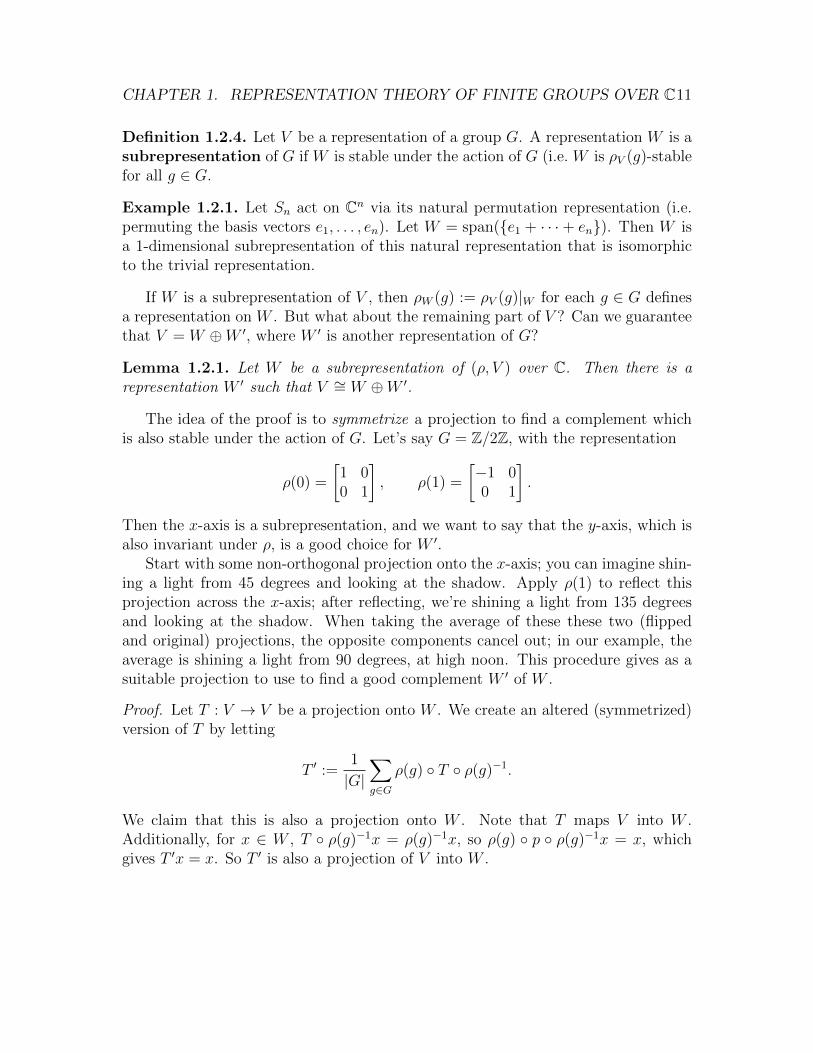
Definition 1.2.4. Let V be a representation of a group G. A representation W is asubrepresentation of G if W is stable under the action of G (i.e. W is ρV (g)-stablefor all g ∈ G.

Example 1.2.1. Let Sn act on Cn via its natural permutation representation (i.e.permuting the basis vectors e1, . . . , en). Let W = span({e1 + · · ·+ en}). Then W isa 1-dimensional subrepresentation of this natural representation that is isomorphicto the trivial representation.

If W is a subrepresentation of V , then ρW (g) := ρV (g)|W for each g ∈ G definesa representation on W . But what about the remaining part of V ? Can we guaranteethat V = W ⊕W ′, where W ′ is another representation of G?

Lemma 1.2.1. Let W be a subrepresentation of (ρ, V ) over C. Then there is arepresentation W ′ such that V ∼= W ⊕W ′.

The idea of the proof is to symmetrize a projection to find a complement whichis also stable under the action of G. Let’s say G = Z/2Z, with the representation

ρ(0) =

[1 00 1

], ρ(1) =

[−1 00 1

].

Then the x-axis is a subrepresentation, and we want to say that the y-axis, which isalso invariant under ρ, is a good choice for W ′.

Start with some non-orthogonal projection onto the x-axis; you can imagine shin-ing a light from 45 degrees and looking at the shadow. Apply ρ(1) to reflect thisprojection across the x-axis; after reflecting, we’re shining a light from 135 degreesand looking at the shadow. When taking the average of these these two (flippedand original) projections, the opposite components cancel out; in our example, theaverage is shining a light from 90 degrees, at high noon. This procedure gives as asuitable projection to use to find a good complement W ′ of W .

Proof. Let T : V → V be a projection onto W . We create an altered (symmetrized)version of T by letting

T ′ :=1

|G|∑g∈G

ρ(g) ◦ T ◦ ρ(g)−1.

We claim that this is also a projection onto W . Note that T maps V into W .Additionally, for x ∈ W , T ◦ ρ(g)−1x = ρ(g)−1x, so ρ(g) ◦ p ◦ ρ(g)−1x = x, whichgives T ′x = x. So T ′ is also a projection of V into W .


Now let W ′ = ker(T ′). We now just need to show that W ′ is also stable underρ(g) for all g ∈ G. Note that

ρ(g) ◦ T ′ ◦ ρ(g)−1 =1

|G|∑h∈G

ρ(g)ρ(g) ◦ T ◦ ρ(h)−1ρ(g)−1

=1

|G|∑h∈G

ρ(gh) ◦ T ◦ ρ(gh)−1

= T ′,

where we have just reindexed the sum by left multiplication by g. We now haveρ(g) ◦ T ′ = T ′ ◦ ρ(g), so for x ∈ W ′,

T ′ ◦ ρ(g)x = ρ(g) ◦ T ′x = 0.

Hence, ρ(g)x ∈ W ′ = ker(T ′), so W ′ is invariant under ρ(g).To summarize, we have found V = W ⊕W ′, where W and W ′ are invariant under

ρ(g) for all g ∈ G, making W,W ′ subrepresentations of V .

Remark 1.2.2. This result holds for fields other than C, as long as char(F ) - |G|.This is what allows us to safely divide by |G|.

Remark 1.2.3. Here is a simpler proof of the lemma for inner product spaces. Ifwe have an inner product, we can make it invariant under the action of G (i.e.〈v, w〉 = 〈ρ(g)v, ρ(g)w〉 for all g ∈ G) by replacing the inner product by 〈v, w〉G :=

1|G|∑

g∈G 〈ρ(g)v, ρ(g)w〉. Then, if we let W ′ be the orthogonal complement of W

with respect to this G-invariant inner product, W ′ is also stable under the action ofG.

As you might hope, the notion of a representation homomorphism is compatiblewith the notion of subrepresentations. In particular, vector subspaces induced bya representation homomorphism, ker(ϕ) and im(ϕ), are subrepresentations of theirrespective vector spaces.

Proposition 1.2.1. Let ϕ : V → W be a representation homomorphism. Thenker(ϕ) and im(ϕ) are subrepresentations of V and W , respectively.

Proof. We show that for each g ∈ G, ρV (g)(ker(ϕ)) ⊆ ker(ϕ) and ρW (g)(im(ϕ)) ⊆im(ϕ). Fix g ∈ G.


• ρV (g)(ker(ϕ)) ⊆ ker(ϕ): Let v ∈ ker(ϕ). Since ϕ is a representation homomor-phism,

ϕ(ρV (g)v) = ρW (g)ϕ(v) = ρW (g)0 = 0.

So if v ∈ ker(ϕ), then ρV (g)v ∈ ker(ϕ); that is, ρV (g)(ker(ϕ)) ⊆ ker(ϕ).

• ρW (g)(im(ϕ)) ⊆ im(ϕ): Let v ∈ V . Since ϕ is a representation homomorphism,ρW (g)ϕ(v) = ϕ(ρV (g)v) ∈ im(ϕ).

If W is a subrepresentation of V , then there is some basis in which the matricesρV (g) all look like

ρV (g) =

[ρW (g) 0

0 ρW ′(g)

].

We can then think of the notion of breaking down representations into smaller sub-representations. Since the dimension decreases each time we take subrepresentations,this procedure must terminate after finitely many steps. So there have to be subrep-resentations which cannot be broken down any further. What do these look like?

Definition 1.2.5. A representation V of G is irreducible if the only subrepresen-tations of V are {0} and V itself.

Example 1.2.2. Any 1 dimensional representation is irreducible.

Example 1.2.3. S3 has the following two dimensional irreducible representation(which we will not prove the irreducibility of at the moment). If S3 � C3 via thenatural permutation representation, then let W = span({e1 − e2, e2 − e3}). W isirreducible, and if we let W ′ = span({e1 + e2 + e3}), C3 ∼= W ⊕W ′.

Theorem 1.2.1 (Maschke). Let V be a finite dimensional representation over C.Then V admits a decomposition into irreducible representations: V ∼=

⊕ri=1 Vi, where

the Vi are irreducible.

Proof. Proceed by induction on n = dim(V ). If n = 1, then V is irreducible,Now suppose that the theorem is true for representations of dimension ≤ n. Ifdim(V ) = n+ 1, and V is not irreducible, then let W be a nontrivial, proper subrep-resentation. By the previous lemma, V ∼= W ⊕W ′ for some other subrepresentationW ′. Applying the inductive hypothesis to W and W ′ (as dim(W ), dim(W ′) ≤ n)gives a decomposition of V into irreducible representations.


1.2.3 Hom(V,W ), HomG(V,W ), and Schur’s lemma

We can define a representation on Hom(V,W ), the collection of linear transforma-tions T : V → W , as follows.

Definition 1.2.6. Let V,W be representations of G (with associated homomor-phisms ρV , ρW ). Then Hom(V,W ) has the representation defined as follows: ifT : V → W is a linear transformation,

[ρHom(V,W )(g)]T := ρW (g) ◦ T ◦ ρV (g−1).

It turns out that we can express this representation in terms of our previousconstructions:

Proposition 1.2.2. Let V,W be finite dimensional representations of G. ThenHom(V,W ) ∼= V ∗ ⊗W via the isomorphism ϕ : V ∗ ⊗W → Hom(V,W ) defined by

ϕ(f ⊗ w) = (v 7→ f(v)w)

and extended to all of V ∗ ⊗W bilinearly.

In other words, we can view a simple tensor f⊗w as a linear transformation fromV → W as follows: given v ∈ V , f “eats” v and returns the result as the coefficientin front of w.3

Proof. We first need to show that ϕ is invertible. We will find an inverse ψ :Hom(V,W ) → V ∗ ⊗ W . Let {v1, . . . , vn} be a basis of V , and let {v∗1, . . . , v∗n}be the corresponding dual basis. Then define

ψ(T ) =n∑i=1

v∗i ⊗ Tvi.

ψ is linear:

ψ(aT + S) =n∑i=1

v∗i ⊗ (aT + S)vi = an∑i=1

v∗i ⊗ Tvi +n∑i=1

v∗i ⊗ Svi = aψ(T ) + ψ(S).

To show that ψ is the inverse of φ, we check that for T ∈ Hom(V,W ) andf ⊗ w ∈ V ∗ ⊗W ,

ϕ(ψ(T )) = ϕ

(n∑i=1

v∗i ⊗ Tvi

)=

n∑i=1

(v 7→ v∗i (v)Tvi) =

(v 7→ T

(n∑i=1

v∗i (v)vi

))= T,

3The proof of this proposition is notationally hard to follow symbol-pushing. I recommend youtry to prove it yourself and consult the proof here whenever you get stuck.


ψ(ϕ(f ⊗ w)) = ψ((v 7→ f(v)w)) =n∑i=1

v∗i ⊗ f(vi)w =

(n∑i=1

f(vi)v∗i

)⊗ w = f ⊗ w.

So ϕ is an invertible linear transformation.To show that ϕ is an isomorphism of representations, we need to check that

[ρHom(V,W )(g)]T = [ψ−1 ◦ ρV ∗⊗W (g) ◦ ψ]T for all T ∈ Hom(V,W ). If g ∈ G, T ∈Hom(V,W ), and v ∈ V , then

([ψ−1 ◦ ρV ∗⊗W (g) ◦ ψ]T )v =

[ψ−1

(ρV ∗⊗W (g)

(n∑i=1

v∗i ⊗ Tvi

))]v

=

[ψ−1

(n∑i=1

ρV ∗(g)v∗i ⊗ ρW (g)Tvi

)]v

Using the fact that ψ−1 is ϕ,

=n∑i=1

(ρV ∗(g)v∗i )(v) · ρW (g)Tvi

= ρW (g)T

(n∑i=1

(ρV ∗(g)v∗i )(v)vi

)

= ρW (g)T

(n∑i=1

v∗i (ρV (g−1)v)vi

)

For any u ∈ V , u =∑n

i=1 v∗i (u)vi; this is because v∗i (u) is just the coefficient of vi in

the decomposition of u with respect to this basis.

= ρW (g) ◦ T ◦ ρV (g−1)v

= [ρHom(V,W )(g)]Tv.

Let HomG(V,W ) be the collection of representation homomorphisms ϕ : V → W .Just like Hom(V,W ) has structure as a vector space, HomG(V,W ) has structurerelated to the representation structure of Hom(V,W ).

Proposition 1.2.3. HomG(V,W ) is the subspace of Hom(V,W ) of linear maps fixedby the action of G. That is,

A ∈ HomG(V,W ) ⇐⇒ A = ρV (g−1)AρW (g) ∀g ∈ G.


Proof. Recall that ρV , ρW are homomorphisms.

A ∈ HomG(V,W ) ⇐⇒ ρV (g)A = AρW (g) ∀g ∈ G⇐⇒ A = (ρV (g))−1AρW (g) ∀g ∈ G⇐⇒ A = ρV (g−1)AρW (g) ∀g ∈ G.

Moreover, there exists a natural projection of Hom(V,W ) onto HomG(V,W ).

Proposition 1.2.4. Let V,W be representations of G. Then the linear map ϕ :Hom(V,W )→ Hom(V,W ) defined by

ϕT :=1

|G|∑g∈G

ρHom(V,W )(g)T

is a projection from Hom(V,W ) onto HomG(V,W ).

Proof. First, we show that im(ϕ) ⊆ HomG(V,W ). Let S = ϕ(T ), where T ∈Hom(V,W ). Then, for any h ∈ G,

ρHom(V,W )(h)S = ρHom(V,W )(h)ϕT

=1

|G|∑g∈G

ρHom(V,W )(h)ρHom(V,W )(g)T

=1

|G|∑g∈G

ρHom(V,W )(hg)T

Left multiplication of all the elements of G by h just reindexes the sum.

= ϕT

= S.

So S is fixed by the action ofG, meaning S ∈ HomG(V,W ). So im(ϕ) ⊆ HomG(V,W ),as claimed.

On the other hand, suppose that T ∈ HomG(V,W ) (i.e. T is fixed by the actionof G on Hom(V,W )). Then

ϕT =1

|G|∑g∈G

ρHom(V,W )(g)T =1

|G|∑g∈G

T = T.

This shows that Hom(V,W ) ⊆ im(ϕ) and that ϕ2 = ϕ.


The following lemma tells us even more about the structure of HomG(V,W ), inthe case where V and W are irreducible representations. It says that there are barelyany representation homomorphisms between irreducible representations.

Lemma 1.2.2 (Schur). Let V,W be irreducible representations of a group G overC, and let ϕ : V → W be a representation homomorphism between them. Then thereare two cases:

1. If V,W are not isomorphic, then ϕ = 0.

2. If (ρV , V ) = (ρW ,W ), ϕ = λI for some λ ∈ C.

In other words,

HomG(V,W ) ∼=

{span({I}) V ∼= W

{0} V 6∼= W.

Proof. Consider ker(ϕ) and im(ϕ). These are subrepresentations of V and W , re-spectively. Since V and W are irreducible, each of these is either {0} or the wholespace. If ker(ϕ) = V , then ϕ = 0.

Otherwise, ker(ϕ) = {0}, which makes im(ϕ) 6= {0}. Then im(ϕ) = W , so ϕ is alinear bijection between V and W , making V ∼= W .

In this case, if V = W , note that ϕ must have an eigenvalue λ since C is alge-braically closed. This means that ker(ϕ − λI) 6= {0} because ϕ has an eigenvector.ϕ− λI is a representation homomorphism:

ρV (g)(ϕ− λI) = ρV (g)ϕ− λρV (g) = ϕρW (g)− λρW (g) = (ϕ− λI)ρW (g).

So ker(ϕ− λI), a nontrivial subrepresentation of V , equals V . That is, ϕ = λI.

Remark 1.2.4. In the proof, we discussed the case where V = W (actual equality,not just isomorphism). Extending to the case of isomorphism is a bit subtle.4 If wehave V ∼= W , rather than just V = W , then V = ψ(W ) for some representationisomorphism ψ. By the equality case, HomG(V, ψ(W )) = span({I}). Since everyϕ ∈ HomG(V,W ) admits a ψ ◦ ϕ ∈ HomG(V, ψ(W )) (and ψ ◦ ϕ = λI for someλ), we must have that HomG(V,W ) = span({ψ−1}). In this case, we still haveHomG(V,W ) ∼= span({I}); that is, the corresponding statement up to isomorphismis still true.

Remark 1.2.5. This result holds for fields other than C, as long as they are alge-braically closed.

4This is a subtlety I’ve never really seen discussed anywhere. My guess is that it mostly goesunnoticed, since people tend to treat isomorphism as equality in their minds.


1.3 Characters of Representations

1.3.1 Characters and class functions

Representations can be a lot of information to deal with. Here is an extremely usefulreduction which does not give away too much information. We take the trace of therepresentation.5

Definition 1.3.1. Given a representation (ρV , V ) of a group G, the characterχV : G→ C is the function

χV (g) := tr(ρV (g)).

Example 1.3.1. Let Sn � Cn by its natural permutation representation. Whatis the character of this representation? The trace of a permutation matrix is thenumber of fixed points of the permutation. So for all σ ∈ Sn,

χ(σ) = |{1 ≤ i ≤ n : σ(i) = i}|.

Example 1.3.2. Let W be the 2 dimensional irreducible representation of S3 intro-duced in the previous section. Then if τ =

(1 2

)and σ =

(1 2 3

),

ρW (σ) =

[0 −11 −1

], ρW (τ) =

[−1 10 1

].

So we get χW (σ) = −1, χW (τ) = 0, and χW (e) = 2.

Example 1.3.3. The character of the trivial representation, χ(g) = 1 for all g ∈ G,is called the trivial character.

Here is a case where no information is lost in reducing a representation to itscharacter.

Example 1.3.4. If ϕ : G → C× is a homomorphism, we can view ϕ as a 1 dimen-sional representation, where ϕ(g) is thought of as a 1 × 1 matrix. In this case, thecharacter χ = ϕ.

In the same vein, if ρ is a 1-dimensional representation of G, χ(g) = ρ(g) for allg ∈ G, since the trace of a 1× 1 matrix is the entry contained within. In this case,χ is called an abelian character.

5The trace of a matrix is a kind of divine magic, the workings of which have been lost to theages. The immense power of this arcane magic is what makes this part of the theory so nice.


The following proposition should convince you that not so much information islost in general when passing from a representation to its character.

Proposition 1.3.1. Let V be a representation of dimension n. Then

χV (e) = dim(V ).

Proof. The trace of the identity matrix is the number of columns in the matrix. Thisis the dimension of the vector space V .

Actually, characters are a simpler reduction than you would expect at first glance.You only need to know the values of χ on a representative of each conjugacy class ofG.

Definition 1.3.2. A class function is a function on a group G that is constant onconjugacy classes of G.

Proposition 1.3.2. Let (ρV , V ) be a representation and χV be its character. ThenχV is a class function.

Proof. Let a, b ∈ G share the same conjugacy class; then there exists some g ∈ Gsuch that b = gag−1. Since the trace is invariant under conjugation,

χV (b) = tr(ρV (gag−1)) = tr(ρV (g)ρV (a)(ρV (g))−1) = tr(ρV (a)) = χV (a).

Here is how characters play with our vector space constructions of representations.

Proposition 1.3.3. Given representations (ρV , V ), (ρW ,W ) of a group G, ∀g ∈ G,the following identities hold:

χV⊕W (g) = χV (g) + χW (g),

χV⊗W (g) = χV (g)χW (g),

χV ∗(g) = χV (g−1).

If V is a vector space over C, we have

χV ∗(g) = χV (g),

where the bar denotes complex conjugation.


Proof. For the first two identities, consider the block matrix forms of ρV⊕W andρV⊗W :

ρV⊕W (g) =

[ρV (g) 0

0 ρW (g)

],

ρV⊗W (g) =

(ρV (g))1,1 ρW (g) (ρV (g))1,2 ρW (g) · · · (ρV (g))1,n ρW (g)(ρV (g))2,1 ρW (g) (ρV (g))2,2 ρW (g) · · · (ρV (g))2,n ρW (g)

......

. . ....

(ρV (g))n,1 ρW (g) (ρV (g))n,2 ρW (g) · · · (ρV (g))n,n ρW (g)

.For the third identity, recall that ρV ∗(g) = (ρV (g−1))>. Since the trace is invariantunder transposition, the identity follows.

Now suppose V is a vector space over C. G is a finite group, so for each g ∈ G,ρV (g) has finite order. Then for some n ∈ N, (ρV (g))n = I, so the eigenvalues ofρV (g) are n-th roots of unity. Since the sum of the eigenvalues of a linear map is itstrace, χV (g) is the sum of roots of unity, χV (g) = λ1 + · · ·+λn. The trace of ρV (g−1)is then λ−1

1 + · · · + λ−1n . And since the complex conjugate of a root of unity is the

same as the multiplicative inverse (ζ−1 = 1/ζ = |ζ|2/ζ = ζ), we have

χV ∗(g) = χV (g−1) = λ−11 + · · ·+ λ−1

n = λ1 + · · ·+ λn = χV (g).

1.3.2 Orthogonality of characters

We can introduce a Hermitian inner product on the vector space of class functions.

Definition 1.3.3. Let ϕ, ψ : G→ C be class functions. Their inner product is

〈ϕ, ψ〉 =1

|G|∑g∈G

ϕ(g)ψ(g−1) =1

|G|∑g∈G

ϕ(g)ψ(g).

The following theorem is the lynchpin upon which all the nice results of repre-sentation theory rely. In some sense, all of the topics to this point were picked so wecould prove this. After the proof, results will start falling into our laps.

Theorem 1.3.1 (Orthogonality of characters). Let (ρV , V ), (ρW ,W ) be irreduciblerepresentations. Then

〈χV , χW 〉 =

{1 V ∼= W

0 V 6∼= W.


Proof.

(χV , χW ) =1

|G|∑g∈G

χV (g−1)χW (g)

=1

|G|∑g∈G

χV ∗(g)χW (g)

=1

|G|∑g∈G

χV ∗⊗W (g)

=1

|G|∑g∈G

χHom(V,W )(g)

Recalling the definition of character and commuting the trace with sums,

= tr

(1

|G|∑g∈G

ρHom(V,W )(g)

).

Recall that 1|G|∑

g∈G ρHom(V,W )(g) is a projection map Hom(V,W ) → HomG(V,W ).

Applying Schur’s lemma, we have that 1|G|∑

g∈G ρHom(V,W )(g) is a projection map

onto a one dimensional subspace of Hom(V,W ) or it is the zero map; i.e.

1

|G|∑g∈G

ρHom(V,W )(g) =

1 0 · · ·0 0 · · ·...

.... . .

V ∼= W

0 0 · · ·0 0 · · ·...

.... . .

V 6∼= W.

Taking the trace completes the proof.

Corollary 1.3.1. Let V ∼= V1 ⊕ · · · ⊕ Vr be a decomposition into irreducible repre-sentations, and let W be an irreducible representation. Then 〈χV , χW 〉 is the numberof Vi isomorphic to W .

Proof. Since χV = χV1 + · · ·+ χVr ,

〈χV , χW 〉 = 〈χV1 , χW 〉+ · · ·+ 〈χVr , χW 〉 .


In this situation, we say that ni := 〈χV , χW 〉 is the “number of copies of Wcontained in V .”

Corollary 1.3.2. The number of copies of each irreducible representation in V isindependent of the decomposition into irreducible representations.

Proof. This is dependent only on 〈χV , χW 〉 for each irreducible W , which is invariantof the decomposition.

In other words, there is only 1 way to decompose a representation into irreduciblerepresentations.

Corollary 1.3.3. The character χV uniquely determines the representation (ρV , V ).That is, if (ρV ′ , V

′) has the character χV , then V ′ ∼= V .

Proof. Since (ρV ′ , V′) has the character χV , V ′ contains the same number of copies

of each irreducible representation as V . So V ′ and V have the same decompositioninto irreducible representations.

Corollary 1.3.4. 〈χV , χV 〉 = 1 if and only if V is irreducible.

Proof. If V is irreducible, then 〈χV , χV 〉 = 1 by the orthogonality of characters. Con-versely, suppose 〈χV , χV 〉 = 1, and decompose V ∼= V n1

1 ⊕ · · · ⊕ V nrr into irreducible

representations, where ni is the number of copies of Vi in V . Then

1 = 〈χV , χV 〉 =r∑i=1

〈niχVi , niχVi〉 =r∑i=1

n2i .

Since all the ni are positive integers, we must have all ni are 0 except one, which is1. So V ∼= Vi for some irreducible Vi.

Corollary 1.3.5. V is irreducible if and only if V ∗ is irreducible.

Proof. Since V ∗∗ ∼= V , it suffices to show that if V is irreducible, so is V ∗. If V isirreducible, then 〈χV , χV 〉 = 1. So

〈χV ∗ , χV ∗〉 =1

|G|∑g∈G

χV ∗(g)χV ∗(g) =1

|G|∑g∈G

χV (g)χV (g) = 〈χV , χV 〉 = 1,

making V ∗ irreducible, as well.

To conclude the section, here is another interpretation of the inner product ofcharacters.


Proposition 1.3.4. Let V,W be representations of G. Then

〈χV , χW 〉 = dim(HomG(V,W )).

Proof. The dimension of the subspace of Hom(V,W ) fixed by the action of G,dim(HomG(V,W )), is the number of copies of the trivial representation in Hom(V,W )(since in HomG(V,W ), every ρHom(V,W )(g) acts as the identity). So we get

dim(HomG(V,W )) =⟨χtriv, χHom(V,W )

⟩=

1

|G|∑g∈G

χtriv(g)χHom(V,W )(g)

=1

|G|∑g∈G

χV ∗(g)χW (g)

=1

|G|∑g∈G

χV (g)χW (g)

= 〈χV , χW 〉 .

Remark 1.3.1. In particular, the inner product of characters will always be a naturalnumber. This is pretty remarkable; you would not expect that from the definition ofthe inner product!6

1.3.3 The regular representation

Every group can be viewed as a group of symmetries of some set via a group actionG � X. Some groups have a “natural” choice of X that they can act on, such asdihedral groups, each of which acts on the vertices of a polygon. But there is auniversal choice for any group: action of G on itself by left multiplication. If weextend this action to an representation on a vector space, we can learn a lot aboutthe representations of G.

Definition 1.3.4. The group algebra, CG, is the vector space with basis elementslabeled by the elements of G. Multiplication is inherited from multiplication ofelements of g and extended linearly:(∑

g∈G

agg

)(∑h∈G

bhh

):=

∑g,h∈G

agahgh.

6The trace is magic.


Remark 1.3.2. This is the same object as the group ring C[G].

Definition 1.3.5. The regular representation is the vector space CG, with theaction of left multiplication:

ρCG(g)

(∑h∈G

ahh

)=∑h∈G

ahgh.

Since left multiplication by a group element permutes the elements of the group,matrices in the regular representation look like permutation matrices.

Despite seeming like such a large object, the regular representation has a verysimple character.

Proposition 1.3.5. The character of the regular representation is

χCG(g) =

{|G| g = e

0 g 6= e.

Proof. The trace of ρCG(g) is the number of diagonal entries of the matrix of ρCG(g),i.e. the number of h ∈ G such that gh = h. This is 0 if g 6= e and is |G| if g = e.

Corollary 1.3.6. The regular representation contains ni copies of each irreduciblerepresentation Vi, where ni = dim(Vi).

Proof. Using the expression for the character χCG,

〈χCG, χVi〉 =1

|G|∑g∈G

χCG(g)χVi(g) =1

|G||G|χVi(e) = dim(Vi) = ni.

Corollary 1.3.7. Let ni be the dimensions of the irreducible representations of G.

|G| =r∑i=1

n2i .

Proof. On one hand,

〈χCG, χCG〉 =1

|G|∑g∈G

χCG(g)χCG(g) =1

|G||G|2 = |G|.

On the other hand, using the decomposition CG ∼= V n11 ⊕ · · · ⊕ V nr

r and the orthog-onality of characters,

〈χCG, χCG〉 =r∑i=1

r∑j=1

⟨niχVi , njχVj

⟩=

r∑i=1

〈niχVi , niχVi〉 =r∑i=1

n2i .

Setting these expressions equal gives the result.


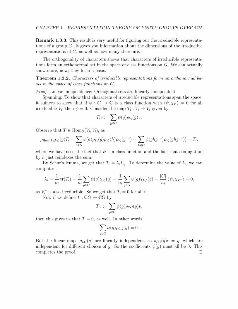
Remark 1.3.3. This result is very useful for figuring out the irreducible representa-tions of a group G. It gives you information about the dimensions of the irreduciblerepresentations of G, as well as how many there are.

The orthogonality of characters shows that characters of irreducible representa-tions form an orthonormal set in the space of class functions on G. We can actuallyshow more, now; they form a basis.

Theorem 1.3.2. Characters of irreducible representations form an orthonormal ba-sis in the space of class functions on G.

Proof. Linear independence: Orthogonal sets are linearly independent.Spanning: To show that characters of irreducible representations span the space,

it suffices to show that if ψ : G → C is a class function with 〈ψ, χVi〉 = 0 for allirreducible Vi, then ψ = 0. Consider the map Ti : Vi → Vi given by

Tiv :=∑g∈G

ψ(g)ρVi(g)v.

Observe that T ∈ HomG(Vi, Vi), as

ρHom(Vi,Vi)(g)Ti =∑h∈G

ψ(h)ρVi(g)ρVi(h)ρVi(g−1) =

∑h∈G

ψ(ghg−1)ρVi(ghg−1)) = Ti,

where we have used the fact that ψ is a class function and the fact that conjugationby h just reindexes the sum.

By Schur’s lemma, we get that Ti = λiIVi . To determine the value of λi, we cancompute:

λi =1

nitr(Ti) =

1

ni

∑g∈G

ψ(g)χVi(g) =1

ni

∑g∈G

ψ(g)χV ∗i (g) =|G|ni

⟨ψ, χV ∗i

⟩= 0,

as V ∗i is also irreducible. So we get that Ti = 0 for all i.Now if we define T : CG→ CG by

Tv :=∑g∈G

ψ(g)ρCG(g)v,

then this gives us that T = 0, as well. In other words,∑g∈G

ψ(g)ρCG(g) = 0.

But the linear maps ρCG(g) are linearly independent, as ρCG(g)e = g, which areindependent for different choices of g. So the coefficients ψ(g) must all be 0. Thiscompletes the proof.


Corollary 1.3.8. The number of irreducible representations of G is equal to thenumber of conjugacy classes of G.

Proof. Let C be the collection of conjugacy classes of G. The space of class functionshas the basis {1Cα : Cα ∈ C}, where

1Cα(g) =

{1 g ∈ Cα0 g /∈ Cα.

So the space of conjugacy classes has dimension |C|. Since characters of irreduciblerepresentations span this space as well, |C| equals the number of irreducible repre-sentations.

As another corollary, we also get another orthogonality relation. We will discussthe interpretation of this in the next section.

Theorem 1.3.3 (2nd orthogonality relation). Let V1, . . . , Vr be the irreducible rep-resentations of G, let g ∈ G, and let Cg be the conjugacy classe of g. Then for anyh ∈ G,

r∑i=1

χVi(h)χVi(g) =

{|G|/|Cg| h ∈ Cg0 h /∈ Cg.

Proof. Consider the class function 1Cg . Since χV1 , . . . , χVr form an orthonormal basisfor class functions on G, we have

1Cg = a1χV1 + · · ·+ arχVr , where ai =⟨1Cg , χVi

⟩.

Writing out the definition of the inner product, we get

ai =1

|G|∑x∈G

1Cg(x)χVi(x) =1

|G|∑x∈Cg

χVi(x) =|Cg||G|

χVi(g).

Plugging these values back into the expression for 1Cg , we get

r∑i=1

χVi(g)χVi =|G||Cg|

1Cg .

Now evaluate both sides at h.


1.3.4 Character tables

Now that we’ve built up the basic theory of representations and characters, we canwork though examples.7 In particular, we can figure out all the characters of irre-ducible representations (and hence all the characters) of G. We will keep track ofthe values of these characters in a character table.

Definition 1.3.6. Let V1, . . . , Vr be the irreducible representations of G, and letg1, . . . , gr be representatives of the conjugacy classes of G. A character table of Gis a matrix A with ai,j = χVi(gj).

Although the character table can be formally thought of as a matrix, we willwrite it out as a table for clarity.

Example 1.3.5. Let’s compute the character table of S3. The conjugacy classes ofS3 correspond to the different cycle types of permutations, so the conjugacy classesare [e], [

(1 2

)], and [

(1 2 3

)]. This also means that we have 3 irreducible repre-

sentations to look for. We have 6 = |S3| =∑3

i=1 n2i , where ni is the dimension of

the i-th irreducible representation, so we must have two 1 dimensional irreduciblerepresentations and one 2 dimensional irreducible representation.

As with all representations, we have the trivial representation. The other 1 dimen-sional representation comes from the sign homomorphism sgn : S3 → {−1, 1} ⊆ C×.So we have two characters already:

χtriv(e) = 1, χtriv((1 2

)) = 1, χtriv(

(1 2 3

)) = 1,

χsgn(e) = 1, χsgn((1 2

)) = −1, χsgn(

(1 2 3

)) = 1.

For the last character, χV3 , we have the choice of a few techniques:

• Solve for the values by using χCG = χtriv + χtriv + 2χV3 .

• Recall that the natural permutation representation Vnat contains a copy of Vtriv:Vnat∼= Vtriv ⊕W for some representation W . Then χW = χnat − χtriv. Since

we know all the 1-dimensional representations, we can check that 〈χW , χtriv〉 =〈χW , χsgn〉 = 0, which tells us that W does not contain any 1-dimensionalrepresentations in its decomposition into irreducibles. Since dim(W ) = 2, Wmust be the irreducible representation we’re looking for.

7I use the word “basic.” but don’t assume I know so much more than this. I wish I did.


• Observe that S3∼= D6, the dihedral group. D6 has a natural 2 dimensional

representation W , by viewing D6 as the symmetries of the plane that fix atriangle. We can then check that 〈χW , χW 〉 = 1, so W is irreducible.

No matter which technique we use, we get the following character table:

S3 [e] [(1 2

)] [(1 2 3

)]

χtriv 1 1 1χsgn 1 −1 1χV3 2 0 −1

Remark 1.3.4. The orthogonality of characters says that the rows of a charactertable are orthogonal. The second orthogonality relation says that the columns areorthogonal.

As the following example shows, computing the character table of an abeliangroup is easier than for a nonabelian group, since we just need to look for 1 dimen-sional representations.

Example 1.3.6. Let’s compute the character table of Z/nZ. Since Z/nZ is abelian,every element is alone in its conjugacy class. So there are n irreducible represen-tations. And since n = |Z/nZ| =

∑ni=1 n

2i , we must have that all the irreducible

representations are 1-dimensional. This means that they all arise from homomor-phisms ϕj : Z/nZ → C×. Since ϕj(k)n = ϕj(nk) = ϕj(0) = 1 for all k ∈ Z/nZ,all elements must be sent to n-th roots of unity. So we get the n homomorphisms,which are determined by what n-th root of unity 1 is sent to:

ϕj(k) = ζkj, where ζ = e2πi/n.

This gives us χj = ϕj = ϕj1, so we get the character table:

Z/nZ 0 1 2 · · · n− 1χtriv = χ0 1 1 1 · · · 1

χ1 1 ζ ζ2 · · · ζn−1

χ2 1 ζ2 ζ4 · · · ζ2(n−1)

......

......

. . ....

χn−1 1 ζn−1 ζ2(n−1) · · · ζ(n−1)2

As groups get larger, the character table generally becomes more difficult todetermine, but the theory we have developed gives enough tools for us to work outsome larger character tables without too much work.


Example 1.3.7. Let’s compute the character table of S4. The conjugacy classes ofS4 correspond to the different cycle types of permutations, so the conjugacy classesare [e], [

(1 2

)], [(1 2 3

)], [(1 2 3 4

)], and [

(1 2

) (3 4

)]. So we need to look

for 5 irreducible representations. As before, we have the characters χtriv and χsgn of1-dimensional representations. And since 24 = |S4| =

∑5i=1 n

2i , we must have n3 = 2

and n4 = n5 = 3 (without loss of generality).There is a normal subgroup N = 〈(1 2)(3 4), (1 3)(2 4)〉 E S4, and S4/N ∼= S3. So

we get representations of S4 by factoring through representations of S3. This givesχ3, which corresponds to the 2-dimensional irreducible representation of S3.

To figure out χ4, recall that we have Vnat∼= Vtriv⊕W for some representation W ,

since the subspace span({e1 + e2 + e3 + e4}) is acted upon trivially in the naturalpermutation representation. We then get χW = χnat − χtriv:

χW (e) = 3, χW ((1 2

)) = 1, χW (

(1 2 3

)) = 0,

χW ((1 2 3 4

)) = −1, χW (

(1 2

) (3 4

)) = −1.

Checking that 〈χW , χW 〉 = 1, we get that χW is the fourth irreducible character.We can now find χ5 by the decomposition of the regular representation:

χCG = χtriv + χsgn + 2χ3 + 3χ4 + 3χ5.

So we get the character table:

S4 e(1 2

) (1 2 3

) (1 2 3 4

) (1 2

) (3 4

)χtriv 1 1 1 1 1χsgn 1 −1 1 −1 1χ3 2 0 −1 0 2χ4 3 1 0 −1 −1χ5 3 −1 0 1 −1

Remark 1.3.5. Instead of using the natural representation to find χ4, we could haveused both orthogonality relations to deduce χ4 and χ5 simultaneously.

Remark 1.3.6. In some cases, such as with the fifth irreducible representation ofS4, it is much easier to figure out the character than it is to find the representa-tion. Nevertheless, there is actually a general theory which gives all the irreduciblerepresentations and charachers of the symmetric groups Sn.

The following proposition will be useful in our next example.


Proposition 1.3.6. The number of 1-dimensional (irreducible) representations of Gis the the order of the abelianization |Gab|.

Proof. Recall that a 1-dimensional representation is a homomorphism ϕ : G→ C×.Since C× is abelian, this homomorphism factors through the abelianization of G:

G C×

Gab

ϕ

ϕ̃

So the number of 1-dimensional representations of G is the number of homomor-phisms ϕ̃ : Gab → C×. That is, the number of 1-dimensional representations of Gis the number of 1-dimensional representations of Gab. Gab is abelian, so every oneof its elements is alone in its own conjugacy class. So there are |Gab| 1-dimensional,irreducible representations of Gab.

Example 1.3.8. Let’s compute the character table of A4. The conjugacy classes ofS4 correspond to the different cycle types of even permutations, but one of the classesgets split in half when passing to A4, since the only permutations which conjugatedelements between these two classes were odd permutations (which are not includedin A4). So the conjugacy classes are [e], [

(1 2 3

)], [(1 3 2

)], and [

(1 2

) (3 4

)].

So we need to look for 4 irreducible representations.To find out the number of 1 dimensional representations, observe that Aab

4∼=

Z/3Z. So the proposition says that there are 3 1 dimensional representations. More-over, since Aab

4 = A4/[G,G] (where [G,G] is the commutator subgroup), we have asurjective homomorphism A4 → Z/3Z. So these 1 dimensional representations arethe representations of Z/3Z, lifted up to A4. So we get χtriv,

χ2(e) = 1, χ2((1 2 3

)) = ζ, χ2(

(1 3 2

)) = ζ2, χ2(

(1 2

) (3 4

)) = 1,

χ3(e) = 1, χ3((1 2 3

)) = ζ2, χ3(

(1 3 2

)) = ζ, χ3(

(1 2

) (3 4

)) = 1,

where ζ = e2πi/3.To find the remaining character, we check 12 = |A4| =

∑4i=1 n

2i , which gives us

that n4 = 3. We can now use the decomposition of the regular representation tosolve for χ4:

χ4 =χCG − χtriv − χ2 − χ3

3.


So we get the character table:

A4 e(1 2 3

) (1 3 2

) (1 2

) (3 4

)χtriv 1 1 1 1χ2 1 ζ ζ2 1χ3 1 ζ2 ζ 1χ4 3 0 0 −1

Example 1.3.9. Let’s compute the character table of

D8 =⟨r, s | s2 = r4 = 1, rs = sr3

⟩.

The conjugacy classes are [e], [s], [r], [rs], and [r2], so we need to find 5 irreduciblerepresentations. Dab

8 = D8/{e, r2} ∼= Z/2Z × Z/2Z, so the four 1 dimensionalrepresentations come from homomorphisms Z/2Z × Z/2Z → C× (with r2 7→ 1).The images of elements in Z/2Z × Z/2Z must have multiplicative order 2, so theymust be 1 or −1. This gives us the four 1 dimensional representations, determinedby whether r and s get sent to 1 or −1.

We now have 8 = |D8| =∑5

i=1 n2i , so n5 = 2. The natural 2 dimensional

representation is the remaining irreducible representation; we can check that it isirreducible by checking the decomposition of the regular representation. So we getthe character table:

D8 e s r rs r2

χ1 1 1 1 1 1χ2 1 −1 1 −1 1χ3 1 1 −1 −1 1χ4 1 −1 −1 1 1χ5 2 0 0 0 −2

Remark 1.3.7. You can check that the quaternion group Q8 has the same charactertable as D8. So a character table does not uniquely determine a group.

Appendix A

Linear Algebra Background

This appendix has far more results than are actually used in the text, but the resultsare interesting in their own right. Also, they are used to develop the theory to thepoint where you are familiar with the objects at hand (which is the whole point ofthe appendix, anyway).

A.1 The trace

In linear algebra, the determinant of matrix gives a lot of useful information aboutthe associated linear transformation. The determinant is a homomorphism det :GLn(C)→ C×, so it tells us about the multiplicative structure of matrices (composi-tion of the linear transformation). This section is about the trace, a homomorphismtr : Mn×n(C)→ C, which tells us about the additive structure of matrices.

Definition A.1.1. Let A be a matrix with entries ai,j. The trace of A is

tr(A) =n∑i=1

ai,i.

Adding together the diagonal entries of a matrix seems arbitrary. But it turnsout that this is a very good quantity to study. From the defnition, we can seetr(A+B) = tr(A) + tr(B). But hte trace has other nice properties. For instance, itis invariant of the choice of basis.

Lemma A.1.1. Let A,B be n× n matrices. Then

tr(AB) = tr(BA).

32

APPENDIX A. LINEAR ALGEBRA BACKGROUND 33

Proof. Write out the definitions of the trace and of matrix multiplication:

tr(AB) =n∑i=1

[AB]i,i =n∑i=1

n∑k=1

ai,kbk,i =n∑k=1

n∑i=1

bk,iai,k =n∑k=1

[BA]k,k = tr(BA).

Proposition A.1.1. The trace is invariant under change of basis. In particular,

tr(A) = tr(BAB−1).

Proof. By the previous lemma,

tr(B(AB−1)) = tr((AB−1)B) = tr(A).

Since the trace is invariant under change of basis, as you might suspect, it has aninterpretation dependent only on the linear transformation, no matrix shenanigansneeded.

Proposition A.1.2. Let A be an n× n matrix over C. Then

tr(A) =n∑i=1

λi,

where the λi are the eigenvalues of A, counted with multiplicity.

Here is a proof, assuming you know about the Jordan canonical form of a matrix.

Proof. Write A in its Jordan canonical form, so A = PJP−1, where J is uppertriangular with the eigenvalues of A long the diagonal. Then

tr(A) = tr(PJP−1) = tr(J) =n∑i=1

λi.

Here is another proof, which does not assume knowledge of the Jordan canonicalform.

Proof. By the fundamental theorem of algebra, the characteristic polynomial of Afactors as cA(t) = (−1)n(t− λ1) · · · (t− λn). When we multiply this out, each termcorresponds to a choice of, for each i, multiplying either a t or a λi; for example, thetn term comes from choosing all the ts, and the constant term comes from choosing


all the −λi. The coefficient of tn−1 in this polynomial is the sum of all the termswhere we only pick one of the λi to multiply. So it is

(−1)n(−λ1 − λ2 − · · · − λn) = (−1)n−1

n∑i=1

λi.

On the other hand, the characteristic polynomial is det(A − tI). If we evaluatethis, we will only get terms with a tn−1 from the product of diagonal entries of A−tI;indeed, any term containing ai,j off the diagonal of A− tI will not contain ai,i− t oraj,j − t, so we can have at most tn−2 in this term. This means that the coefficient oftn−1 in cA(t) = det(A− tI) is the coefficient of tn−1 in (a1,1− t)(a2,2− t) · · · (an,n− t).By the same argument as above, this coefficient is

(−1)n−1(a1,1 + a2,2 + · · ·+ an,n) = (−1)n−1 tr(A).

These two expressions are both the coefficient of tn−1 in the characteristic poly-nomial of A, so they are equal. We get

tr(A) =n∑i=1

λi.

Here are some vague thoughts to help you interpret the trace: What does adiagonal element of a matrix refer to? If we fix a basis {v1, . . . , vn} of V , ai,i is howmuch in the direction of vi Avi is. If we assume this to be an orthonormal basis,ai,i = 〈Avi, vi〉. The trace is invariant under change of basis, and we can think of thisin the sense of “if we sum the amount that A keeps vectors in the same direction, butin every direction, we should get an quantity invariant of which vectors we pickedfor our directions.”

On the other hand, the trace is also the sum of the eigenvalues (with multiplic-ities). In this sense, the picture is even cleaner. The trace is the sum of how muchA keeps vectors in the same direction, for every direction. In the case where youhave a basis of eigenvectors, Avi is now entirely in the direction of vi. So the trace isreally just a measure of how much A moves or does not move vectors into a differentdirection from where they started.


A.2 Products and Direct sums

The Cartesian product is a way of combining sets to get ordered pairs of elementsbetween sets:

A×B := {(a, b) : a ∈ A, b ∈ B}.For infinite products (indexed by some infinite set I), we get something that lookslike this: ∏

α∈I

Aα := {(aα)α∈I : aα ∈ Aα ∀α ∈ I}.

In a similar way, we can construct a product of vector spaces.

Definition A.2.1. If Vα are vector spaces, the product∏

α∈I Vα is a vector spacewith componentwise addition and scalar multiplication:

c(aα)α∈I + (bα)α∈I = (caα + bα)α∈I .

As you can imagine, products can be very large. Even if Vα = Q, viewed asa vector space over Q, we can get uncountable products by taking a product ofuncountably many such Vα. However, there is another way to combine spaces whichproduces spaces which are not as large.

Definition A.2.2. If Vα are vector spaces, the direct sum⊕

α∈I Vi is the followingsubspace of

∏α∈I Vα:⊕α∈I

Vα := {(aα)α∈I : aα = 0 for all but finitely many α}.

Remark A.2.1. For finite direct sums, the definition is the same as the product:

V1 ⊕ · · · ⊕ Vn = V1 × · · · × Vn.

The direct sum is not such an unfamiliar concept. Here is an example you arealready familiar with.

Example A.2.1. Let P be the collection of polynomials with coefficients in C. Thisis a vector space over C. By looking at the coefficients of a polynomial, polynomials inP look like ordered tuples of coefficients (which can be 0); for example, the polynomial5x3−

√2x+i can be thought of as the sequence (i,−

√2, 0, 5, 0, . . . ). Every polynomial

only has finitely many nonzero terms, so

P ∼=∞⊕j=1

C.


This is not the same as∏∞

j=1 C. In the product, we have elements such as

(1, 1, 1, . . . ), which correspond to power series such as 1 + x + x2 + · · · . These arenot polynomials, though. In this case, the product,

∏∞j=1 C is the vector space of

formal power series1 with coefficients in C.

1The word formal here indicates that we only care about the symbols, without any regard towhether these series actually converge.


A.3 Dual spaces

Dual spaces are a common construction in advanced linear algebra.

Definition A.3.1. Let V be a vector space over a field F . Then the dual vectorspace V ∗ is the vector space of linear functions T : V → F .

Remark A.3.1. At first glance, this definition seems fairly arbitrary and unmoti-vated. Here’s why we care about dual spaces. One of the central ideas of functionalanalysis is the study of (infinite dimensional) vector spaces of functions, such asC([0, 1]) = {f : [0, 1] → R | f is continuous}. In this setting, many familiar func-

tions are elements of the dual space, such as the integration map: T (f) :=∫ 1

0f(x) dx.

Here is a way for us to talk about vectors in the dual space.

Proposition A.3.1. Let V be a finite dimensional vector space with basis {v1, . . . , vn}.Then {v∗1, . . . , v∗n} is a basis for V ∗, where

v∗i (vj) =

{1 j = i

0 j 6= i.

Proof. Let v∗i be defined as above; that is, for each i,

v∗i (a1v1 + · · ·+ anvn) = ai.

The v∗i are linearly independent: if a1v∗1 + · · ·+ anv

∗n = 0, then for each i,

0 = a1v∗1(vi) + · · ·+ anv

∗n(vi) = ai.

So all the ai equal 0.To see that the v∗i span V ∗, let f ∈ V ∗. Since f is linear and V is finite dimen-

sional, f is uniquely determined by f(vi) for 1 ≤ i ≤ n. Letting ai = f(vi) for eachi, we get that

f = a1v∗1 + · · ·+ anv

∗n,

as these agree when applied to each of the vi.

Linear maps between vector spaces give rise to linear maps between dual spaces.

Definition A.3.2. Given a linear map T : V → W , the induced dual map T ∗ :W ∗ → V ∗ is given by f 7→ f ◦ T .

V W

V ∗ W ∗

T

T ∗


Here’s why this construction is called the “dual” space.

Proposition A.3.2. If T : V → W is a linear transformation with matrix A, thenthe dual map T ∗ : W ∗ → V ∗ has matrix representation A>.

Proof. Let {v1, . . . , vn} and {w1, . . . , wm} be ordered bases of V and W , respectively.Let {v∗1, . . . , v∗n} and {w∗1, . . . , w∗m} be the corresponding dual bases. We have that

(T ∗w∗i )

(n∑j=1

bjvj

)= w∗i

(n∑j=1

bjTvj

)

= w∗i

(n∑j=1

bj

m∑k=1

ak,jwk

)

=n∑j=1

m∑k=1

bjak,j w∗i (wk)︸︷︷︸δi,k

=n∑j=1

bjai,j

=n∑j=1

ai,jv∗j

(n∑`=1

b`v`

),

so T ∗w∗i =∑n

j=1 ai,jv∗j . The definition of matrix multiplication gives us [T ∗]j,i = ai,j,

and we are done.

Here’s the picture: if vectors in V are column vectors, then vectors in the dualspace are row vectors. In the vector space V , matrices act on the left as Av. In thedual space, matrices act on the right, and the action of the corresponding matrix forthe dual transformation looks like v∗A>, where v∗ is a row vector.

In this picture, what does v∗i (vj) look like? If these are the basis vectors for theirrespective spaces, we get δi,j. This agrees with multiplication of the vectors v>i vj:

v∗i (vj) =[

vi] vj

.Now notice that if we fix v∗i , this becomes linear in v if we replace vj by any v ∈ V .Correspondingly. if we fix vj, this is linear in f if we replace v∗i by any f ∈ V ∗. So,


in general, f(v) gives the same value as multiplication of the vectors f>v:

f(v) =[

f] v

.For this reason, if v ∈ V and f ∈ V ∗, we often denote f(v) as the pairing 〈v, f〉.With this notation, the action of matrices looks like

〈Av, f〉 = f(Av) = (A∗f)(v) = 〈v,A∗f〉 .

This gives an analogy between the relationship between a vector and its dual spaceand the relationship between an inner product space and itself.

Warning A.3.1. This should not be confused with the concept of a Hermitian innerproduct; with a Hermitian inner product on a complex vector space, the adjoint A†

of A satisfies 〈Av,w〉 = 〈v, A†w〉, but the matrix of the adjoint is the conjugatetranspose of A, not just the transpose.


A.4 Tensor products of vector spaces

The tensor product is a way of “combining vector spaces in a bilinear manner.” Hereis a motivating example.

Example A.4.1. Consider the vector space Pn of polynomials of degree ≤ n withcoefficients in C. Suppose we want to construct a space of polynomials in 2 variables,x and y, of x-degree ≤ n and y-degree ≤ n. Your first guess might be to try to usePn ⊕ Pn, but this has dimension 2(n + 1); the desired space of polynomials in 2variables should have dimension (n+ 1)2.

Now observe that we can obtain polynomials in 2 variables in the following way:take polynomials f(x) and g(y), and multiply them. This gives another reasonwhy Pn ⊕ Pn would not work. If we tried to identify (f(x), g(y)) as the polynomialf(x)g(y), we run into the problem of how scalar multiplication works; a(f(x), g(y)) =(af(x), ag(y)), but a · f(x)g(y) is not (af(x))(ag(y)). This issue arises because themap (f(x), g(y)) 7→ f(x)g(y) is bilinear, rather than linear; in particular, scalarmultiplication works separately, in each of the two coordinates of (f(x), g(y)).

We want to find a method of combining these vector spaces so that the end resultcan take this bilinear map and interpret it as a linear map (since a single vectorspace should work with linear maps). The tensor product, Pn⊗Pn will be the spacewe want.

Definition A.4.1. Let V and W be vector spaces over F . A map T : V ×W isbilinear if T (·, w) and T (v, ·) are linear for each v ∈ V and w ∈ W . T is calledF -balanced if T (av, w) = T (v, aw) for all a ∈ F .

Example A.4.2. Let V be an inner product space over R. Then 〈·, ·〉 : V × V → Ris a bilinear and R-balanced; it is linear in each of the individual entries. Is there avector space related to V ×V where we can view the inner product as a linear map?The tensor product, V ⊗ V , will give us the solution.

To construct the tensor product of V and W , we want to combine V and W ina way such that scalars act in both coordinates of (v, w). How do we construct suchan object? The answer is basically “just do it.”

Definition A.4.2. The tensor product of vector spaces V and W (over a field F ),denoted V ⊗W (or V ⊗F W ), is the quotient

⊕(v,w)∈V×W F (v, w)/Z, where Z is the

subspace generated by all elements of the form

1. (v + v′, w)− (v, w)− (v′, w)


2. (v, w + w′)− (v, w)− (v, w′)

3. (av, w)− (v, aw)

for all v, v′ ∈ V , w,w′ ∈ W , and a ∈ F . The image of (v, w) in V ⊗W is denoted asv ⊗ w and called a simple tensor.

Let’s unpack this; what does this definition mean? We start with a a huge vectorspace with a basis given by all possible linear combinations of pairs (v, w) ∈ V ⊗W );this has everything we want, but also a lot more. To establish the relations ofbilinearity, we quotient out by corresponding elements. In other words, since in thisquotient, (v + v′, w)− (v, w)− (v′, w) = 0, we get the relation that

(v + v′, w) = (v, w) + (v′, w).

So the inclusion of the first two types of elements in Z enforces the condition that inthe quotient, we can split up elements linearly in each component. Similarly, sincein this quotient, (av, w)− (v, aw) = 0, we get that

(av, w) = (v, aw).

So scalar multiplication acts individually in each component (and can “pass fromone component to the other”).

In summary, we have just taken a huge space which contains the space we wantand enforced the relations we want.2

Let’s take a look at what this space looks like.

Example A.4.3. Consider V ⊗W over C. We have simple tensors, (v, w), and alsolinear combinations of simple tensors, such as

4(v1 ⊗ w1) +√

3(v2 ⊗ w2) + (5− i)(v1 ⊗ w3).

Here, 4(v1 ⊗ w1) means (4v1) ⊗ w1 or v1 ⊗ (4w1) (these are equal). Since the firstand third terms both have v1 in the first component, we can combine them:

= v1 ⊗ (4w1) +√

3(v2 ⊗ w2) + v1 ⊗ (5− i)w3

= v1 ⊗ (4w1 + (5− i)w3) +√

3(v2 ⊗ w2).

2Enforcing these relations by quotienting out by the proper subspace is a really clever idea.


Example A.4.4. Here are some more examples of how simple tensors work, so youcan get used to them. Let k ∈ Z. Then

k(v ⊗ w) = (v ⊗ w) + · · ·+ (v ⊗ w) = (v + · · ·+ v)⊗ w) = (kv)⊗ w.

Similarly,k(v ⊗ w) = v ⊗ (kw).

If the field F contains Z, then this is consistent with our relation of scalar multipli-cation:3

(kv)⊗ w = v ⊗ (kw).

We also have(−1)(v ⊗ w) = (−v)⊗ w = v ⊗ (−w),

0⊗ w = (0v)⊗ w = 0(v ⊗ w) = 0,

v ⊗ 0 = 0⊗ w = 0.

Warning A.4.1. It is a really common mistake to think of consider simple tensorsas the only elements of the tensor product. Do not do this. The tensor product hasall linear combinations of simple tensors as its elements. Sometimes, terms can besimplified into fewer simple tensors, but this is not always the case.

Example A.4.5. Consider R2 ⊗ R2. We cannot simplify the term

(1, 0)⊗ (0, 1) + (0, 1)⊗ (1, 0)

into a single simple tensor. In general, elements of the form

v1 ⊗ w1 + v2 ⊗ w2

with v1 6= v2 and w1 6= w2 cannot be written as a single simple tensor.

There is always a map V ×W → V ⊗W given by (v, w) 7→ v⊗w. This map is notsurjective (as was just warned). This is how the tensor product “converts bilinearmaps into linear maps.”

Proposition A.4.1 (tensor product universal property). Let V,W,X be vector spacesand φ : V ×W → X be such that

3If F does not contain Z, then kv is interpreted in the sense of kv := v + · · ·+ v, where we addup k of these.


1. φ(v + v′, w) = φ(v, w) = φ(v′, w) (left biadditivity),

2. φ(v, w + w′) = φ(v, w) + φ(v, w′) (right biadditivity),

3. φ(av, w) = φ(v, aw) (F -balanced),

for all v, v′ ∈ V , w,w′ ∈ W , and a ∈ F . There exists a unique linear map Φ :V ⊗W → X such that Φ(v ⊗ w) = φ(v, w) for all v ∈ V and w ∈ W .

V ×W X

V ⊗W

φ

Φ

Proof. Given φ, define

Φ

(n∑i=1

ai(vi ⊗ wi)

):=

n∑i=1

aiφ(vi, wi).

The conditions on φ guarantee that this map is well-defined; i.e. it matters not whatlinear combination we use to express the input (if there is more than 1 that works).This map is linear by definition and satisfies Φ(v ⊗ w) = φ(v, w) (this is the casewhere n = 1 and a1 = 1).

For uniqueness, let Ψ : V ⊗W → X be another linear map such that Ψ(v⊗w) =φ(v, w) for all v ∈ V and w ∈ W . Using the linearity of Ψ, we get that

Ψ

(n∑i=1

ai(vi ⊗ wi)

)=

n∑i=1

aiφ(vi, wi).

So Ψ = Φ.

Remark A.4.1. This is often taken to be the “real definition” of the tensor product,as in “a tensor product is anything that satisfies this universal property.” From thispoint of view, our construction from before would be the proof of a theorem thatsuch an object exists. One reason why people prefer this definition is that it is theeasiest way to prove basically every property of the tensor product.

Basically, you always want to use the universal property when proving somethinginvolving tensor products. Here is an example.


Proposition A.4.2. Let Pn,n be the vector space of polynomials in 2 variables, xand y, of x-degree ≤ n and y-degree ≤ n, and let Pn be the vector space of singlevariable polynomials of degree ≤ n. Then Pn ⊗ Pn ∼= Pn,n.

The idea is that we use the universal property to construct a linear map Φ :Pn ⊗ Pn → Pn,n and then find an inverse.

Proof. Consider the map φ : Pn × Pn → Pn,n sending (f(x), g(y)) 7→ f(x)g(y). Thisis bilinear and C-balanced, so by the universal property of the tensor product, thereexists a linear map Φ : Pn ⊗ Pn → Pn,n such that Φ(f(x)⊗ g(y)) = f(x)g(y).

To show that Φ is an isomorphism, we find an inverse Ψ : Pn,n → Pn⊗Pn. Define

Ψ

(n∑

i,j=0

ai,jxiyj

)=

n∑i,j=0

ai,j(xi ⊗ yj).

By definition, Ψ is a linear map. We check that Φ and Ψ are inverses:

Φ ◦Ψ

(n∑

i,j=0

ai,jxiyj

)= Φ

(n∑

i,j=0

ai,j(xi ⊗ yj)

)=

n∑i,j=0

ai,jxiyj.

To check the other way, we want to show that Ψ ◦Φ is the identity on Pn⊗Pn. Notethat since Φ and Ψ are linear, Ψ◦Φ is linear. So it suffices to just check that Ψ◦Φ isacts as the identity when applied to simple tensors. Moreover, by splitting up termsbilinearly (like (x + 2x2) ⊗ y4 = x ⊗ y4 + 2x2 ⊗ y4), it suffices to check that Ψ ◦ Φacts as the identity when applied to terms of the form xi ⊗ yj:

Ψ ◦ Φ(xi ⊗ yj

)= Ψ

(xiyj

)= xi ⊗ yj.

So Φ : Pn ⊗ Pn → Pn,n is a linear map with an inverse. That is, Pn ⊗ Pn ∼= Pn,n, asdesired.

Remark A.4.2. Whenever you want to prove that something can be described by atensor product (i.e. it is isomorphic to a tensor product of something), the proof willproceed almost exactly as above. When you want to prove that Φ is invertible, it’susually possible to show that it is surjective. But showing that it is injective usuallyends up being pretty intractable. So try to always use the universal property andthen find an inverse.

In the above example, Pn had a basis of {1, x, . . . , xn}, and Pn,n had a basis of{1, x, . . . , xn, y, xy, . . . , xny, y2, . . . , xnyn} That is, we obtained a basis for Pn,n bytaking pairs of basis elements of Pn. This gives us a general way to find a basis ofV ⊗W in terms of a bases of V and W .


Proposition A.4.3. Let V and W be vector spaces over F with ordered bases{v1, . . . , vn} and {w1, . . . , vm}, respectively. Then V ⊗W has the basis

B = {vi ⊗ wj : 1 ≤ i ≤ n, 1 ≤ j ≤ m}.

Proof. B spans V ⊗W : It sufficces to show that B contains all simple tensors. Letv ⊗ w ∈ V ⊗W . Then express

v ⊗ w =

(n∑i=1

aivi

)⊗

(m∑j=1

bjwj

)=

n∑i=1

m∑j=1

aibj(vi ⊗ wj).

As each vi ⊗ wj is in B, v ⊗ w is in the span of B.B is linearly independent: Suppose that

∑ni=1

∑mj=1 ci,j(vi⊗wj) = 0. We want to

show that ck,` = 0 for each ordered pair (k, `). Consider the map φk,` : V ×W → Fgiven by

φi,j

(n∑i=1

aivi,m∑j=1

bjwj

)= akb`.

The map φk,` is bilinear and F -balanced, so by the universal property of the tensorproduct, there is a linear map Φk,` : V ⊗W → F such that

Φk,`

((n∑i=1

aivi

)⊗

(m∑j=1

bjwj

))= akb`.

Now observe that

Φk,`

(n∑i=1

m∑j=1

ci,j(vi ⊗ wj)

)= ck,`.

On the other hand, since∑n

i=1

∑mj=1 ci,j(vi ⊗ wj) = 0,

Φk,`

(n∑i=1

m∑j=1

ci,j(vi ⊗ wj)

)= Φk,`(0) = 0.

This holds for any (k, `), so all the ck,` = 0.

Corollary A.4.1. If dim(V ) = n and dim(W ) = m, then dim(V ⊗W ) = nm.

Proof. The basis {vi ⊗ wj : 1 ≤ i ≤ n, 1 ≤ j ≤ m} of V ⊗W has nm elements.


This gives a good reasoning for the notation ⊗ for the tensor product. This is away to “multiplicatively” combine two vector spaces. For example, if V is a vectorspace with basis {} and W is a vector space with basis {}, then V ⊗W is a basiswith vector space {}

Here are some more properties of tensor products. If you can follow the proofswell, then you should have a good enough understanding of the tensor product. First,the tensor product is symmetric:

Proposition A.4.4. Let V,W be vector spaces over F . Then V ⊗W ∼= W ⊗ V .

Proof. Let φ : V ×W → W ⊗ V send (v, w) 7→ w ⊗ v. The map φ is bilinear andF -balanced, so by the universal property of the tensor product, there is a linear mapΦ : V ⊗W → W ⊗ V such that Φ(v ⊗ w) = w ⊗ v.

To show that Φ is an isomorphism, we show that it has an inverse. If we make thesame construction, we get a linear map Ψ : W ⊗ V → V ⊗W such that Ψ(w⊗ v) =v ⊗ w. To show that these are inverses, by the linearity of Φ and Ψ, it suffices toshow that Ψ ◦ Φ and Φ ◦Ψ act as the identity on simple tensors. We have:

Ψ ◦ Φ(v ⊗ w) = Ψ(w ⊗ v) = v ⊗ w,

Φ ◦Ψ(w ⊗ v) = Ψ(v ⊗ w) = w ⊗ v.So Φ : V ⊗W → W ⊗ V is an isomorphism.

Tensoring by the base field (or equivalently a 1-dimensional vector space) doesnothing.

Proposition A.4.5. Let V be a vector space over F . Then V ⊗ F ∼= V .

Proof. Let φ : V × F → V send (v, a) 7→ av. This is bilinear and F -balanced, so byuniversal property of the tensor product, there is a linear map Φ : V ⊗ F → V suchthat Φ(v ⊗ a) = av.

To show that Φ is an isomorphism, we find an inverse. Consider the linear mapΨ : V → V ⊗ F sending v 7→ (v, 1). We have

Φ ◦Ψ(v) = Φ(v ⊗ 1) = v.

For the reverse composition, by the linearity of Φ and Ψ, it suffices to show thatΨ ◦ Φ is the identity on simple tensors. We have

Ψ ◦ Φ(v ⊗ a) = Ψ(av) = (av)⊗ 1 = v ⊗ a.

So Φ is the desired isomorphism.


Tensor products distribute over direct sums.

Proposition A.4.6. Let Vα, α ∈ I and W be vector spaces over F . Then(⊕α∈I

Vα

)⊗W ∼=

⊕α∈I

(Vα ⊗W ).

Proof. Let ψ :(⊕

α∈I Vα)×W →

⊕α∈I(Vα ⊗W ) send ((vα)α∈I , w) 7→ (vα ⊗ w)α∈I .

This is bilinear and F -balanced, so by universal property of the tensor product, thereis a linear map Φ :

(⊕α∈I Vα

)⊗W →

⊕α∈I(Vα ⊗W ) such that Φ((vα)α∈I ⊗ w) =

(vα ⊗ w)α∈I .To show that Φ is an isomorphism, we find an inverse. Consider the bilinear,

F -balanced maps ψα : Vα ×W → (⊕

α∈I Vα)⊗W sending (vα, w) 7→ vα ⊗ w, wherevα ∈

⊕α∈I Vα has all components 0, except vα in the α-th component. By the

universal property of the tensor product, there are linear maps Ψα : Vα ⊗ W →(⊕

α∈I Vα) ⊗ W such that Ψα(vα ⊗ w) = vα ⊗ w for each α. Now construct Φ :⊕α∈I(Vα ⊗W ) →

(⊕α∈I Vα

)by Φα =

∑α∈I Φα. This is well-defined because for

any input, only finitely many vα are nonzero, so we area only ever adding up finitelymany images of the Φα at a time.

By the linearity of Φ and Ψ, it suffices to check that they are inverses of eachother on simple tensors. We have

Ψ ◦ Φ((vα)α∈I ⊗ w) = Ψ((vα ⊗ w)α∈I) = (vα)α∈I ⊗ w,

Φ ◦Ψ((vα ⊗ w)α∈I) = Φ((vα)α∈I ⊗ w) = (vα ⊗ w)α∈I .

So Φ is the desired isomorphism.

We finish the section with an explanation of how linear maps interact with thetensor product.

Definition A.4.3. Let T : V → X and S : W → Y be linear maps. The tensorproduct of linear maps S ⊗ T : V ⊗W → X ⊗ Y is the the unique linear mapgiven by (S ⊗ T )(v ⊗ w) := Tv ⊗ Sw.

Proposition A.4.7. T ⊗ S exists (and is unique).

Proof. Consider the bilinear, F -balanced map φ : V ×W → X⊗Y given by (v, w) 7→Tv ⊗ Sw. By the universal property of the tensor product, there is a unique linearmap Φ : V ⊗W → X⊗Y such that Φ(v⊗w) = Tv⊗Sw. Φ is the map we want.


Suppose A and B are matrices. What does the matrix of A⊗B look like? Orderthe basis of V ⊗W lexicographically:

{v1 ⊗ w1, . . . , v1 ⊗ wm, v2 ⊗ w1, . . . , v2 ⊗ wm, . . . , vn ⊗ wm}.

Since (A ⊗ B)(vi ⊗ wj) = Avi ⊗ Bwj, the (k, `) coefficient of (A ⊗ B)(vi ⊗ wj) isai,kb`,j. So with this ordering of the basis, the matrix of A⊗B (in block matrix form)looks like

a1,1 B a1,2 B · · · a1,n Ba2,1 B a2,2 B · · · a2,n B...

.... . .

...an,1 B an,2 B · · · an,n B

.Example A.4.6. Recall our proof that if V has basis {v1, . . . , vn} and W has basis{w1, . . . , wm}, then V ⊗W has the basis {vi ⊗ wj : 1 ≤ i ≤ n, 1 ≤ j ≤ m}. We hada map Φk,` such that

Φk,`

(n∑i=1

m∑j=1

ci,j(vi ⊗ wj)

)= ck,`.

In hindsight, we can see that this map is a member of the dual basis of V ⊗W . Infact, we can construct it as a tensor product of linear maps:

Φk,` = v∗k ⊗ w∗` ,

where v∗k and w∗` are members of the dual bases of V ∗ and W ∗, respectively. Here,the codomain is F ⊗ F ∼= F .

This recipe tells us something about dual spaces and tensor products, in general.

Proposition A.4.8. Let V,W be finite dimensional vector spaces over F . Then

V ∗ ⊗W ∗ ∼= (V ⊗W )∗.

Proof. Consider the map ψ : V ∗ ×W ∗ → (V ⊗W )∗ given by (T, S) 7→ T ⊗ S (here,T ⊗ S is a linear functional because F ⊗ F ∼= F ). The map ψ is bilinear and F -balanced, so by the universal property of the tensor product, there is a linear mapΦ : V ∗ ⊗W ∗ → (V ⊗W )∗ such that Φ(T ⊗ S) = T ⊗ S (the second usage meaningthe tensor product of linear maps).

The map Φ is injective. Suppose Φ(T ⊗ S) = 0. Then (Tv) · (Sw) = 0 for allv. This means that either Tv = 0 for all v ∈ V or Sw = 0 for all w ∈ W ; i.e.either T = 0 or S = 0. But then T ⊗ S = 0, meaning that ker(Φ) = {0}. SoΦ is injective. Since V ∗ ⊗W ∗ and (V ⊗W )∗ are finite dimensional with the samedimension (dim(V ) · dim(W )), Φ is also surjective. So Φ is an isomorphism.


Remark A.4.3. This is not true for infinite dimensional vector spaces, since thedual of an infinite dimensional vector space is much bigger than the space itself.

Bibliography

[FH13] W. Fulton and J. Harris. Representation Theory: A First Course. GraduateTexts in Mathematics. Springer New York, 2013.

[SS12] L.L. Scott and J.P. Serre. Linear Representations of Finite Groups. GraduateTexts in Mathematics. Springer New York, 2012.

50

Representation Theory - GitHub Pages Notes/Representation Theory... · Representation theory, at...

Documents

Transcript of Representation Theory - GitHub Pages Notes/Representation Theory... · Representation theory, at...