Reported Incomes and Marginal Tax Rates, 1960-2000 ...saez/saezTPE04.pdf · REPORTED INCOMES AND...
57
REPORTED INCOMES AND MARGINAL TAX RATES, 1960-2000: EVIDENCE AND POLICY IMPLICATIONS Emmanuel Suez University of California and NBER EXECUTIVE SUMMARY This paper uses income tax return data from 1960 to 2000 to analyze the link between reported incomes and marginal tax rates. Only the top 1 per cent of income earners show evidence of behavioral responses to taxation. The data display striking heterogeneity in the size of responses to tax changes over time, with no response either short-term or long-term for the very large Kennedy top income tax cuts in the early 1960s, and strik ing evidence of responses, at least in the short term, to the tax changes since the 1980s. The 1980s tax cuts generated a surge in business income reported by high-income individual taxpayers, due to a shift away from the corporate sector, and the disappearance of business losses for tax avoidance. The Tax Reform Act of 1986 and the recent 1993 tax increase generated large short-term responses of wages and salaries reported by top income earners most likely because of retiming in compensation to take advantage of the tax changes. It is unlikely, however, that the extraor dinary trend upward of the shares of total wages accruing to top wage income earners, which started in the 1970s and accelerated in the 1980s and especially the late 1990s, can be explained solely by the evolution of marginal tax rates. I am very grateful to Dan Feenberg for his help using the micro tax return data and the TAXSIM calculator. I thank Alan Auerbach, Gerald Auten, Robert Carroll, Dan Feenberg, Martin Feldstein, Wojciech Kopczuk, Andrew Leigh, Thomas Piketty, James Poterba, and especially Joel Slemrod for very helpful comments and discussions. Financial support from the Sloan Foundation and NSF Grant SES-0134946 is gratefully acknowledged.
Transcript of Reported Incomes and Marginal Tax Rates, 1960-2000 ...saez/saezTPE04.pdf · REPORTED INCOMES AND...
REPORTED INCOMES AND
MARGINAL TAX RATES, 1960-2000: EVIDENCE AND
POLICY IMPLICATIONS
Emmanuel Suez University of California and NBER
EXECUTIVE SUMMARY
This paper uses income tax return data from 1960 to 2000 to analyze the
link between reported incomes and marginal tax rates. Only the top 1 per cent of income earners show evidence of behavioral responses to taxation.
The data display striking heterogeneity in the size of responses to tax
changes over time, with no response either short-term or long-term for
the very large Kennedy top income tax cuts in the early 1960s, and strik
ing evidence of responses, at least in the short term, to the tax changes since the 1980s. The 1980s tax cuts generated a surge in business income
reported by high-income individual taxpayers, due to a shift away from
the corporate sector, and the disappearance of business losses for tax
avoidance. The Tax Reform Act of 1986 and the recent 1993 tax increase
generated large short-term responses of wages and salaries reported by top income earners most likely because of retiming in compensation to
take advantage of the tax changes. It is unlikely, however, that the extraor
dinary trend upward of the shares of total wages accruing to top wage income earners, which started in the 1970s and accelerated in the 1980s
and especially the late 1990s, can be explained solely by the evolution of
marginal tax rates.
I am very grateful to Dan Feenberg for his help using the micro tax return data and the
TAXSIM calculator. I thank Alan Auerbach, Gerald Auten, Robert Carroll, Dan Feenberg, Martin Feldstein, Wojciech Kopczuk, Andrew Leigh, Thomas Piketty, James Poterba, and
especially Joel Slemrod for very helpful comments and discussions. Financial support from the Sloan Foundation and NSF Grant SES-0134946 is gratefully acknowledged.
118 Saez
1. INTRODUCTION
Over the last 40 years, the U.S. federal income tax system has undergone
large changes. Perhaps the most striking change has been the dramatic
decrease in top marginal income tax rates. From 1950 to the early 1960s, the statutory top marginal income tax rate was 91 percent. This rate was
reduced to 70 percent by the Kennedy tax cuts in the mid-1960s. During the Reagan administrations of the 1980s, the top income tax rate was fur
ther reduced to 50 percent in 1982 by the Economic and Recovery Tax Act
(ERTA) of 1981, and was reduced again to 28 percent in 1988 by the Tax
Reform Act (TRA) of 1986. The top income tax rate was then increased to
31 percent in 1991 and further to 39.6 percent in 1993 by the Omnibus
Budget Reconciliation Act (OBRA) of 1993. The top rate has been reduced
to 35 percent in 2003 by the 2001 tax reform. Only about 500 taxpayers were subject to the top marginal tax rate of 91 percent in the early 1960s, but by 2000, more than half a million taxpayers were subject to the top rate.1 Thus, the continuous and drastic progressivity of the federal income
tax system up to the very highest income taxpayers has been replaced by a much flatter tax structure, where an upper-middle-class family can face
the same marginal tax rate as the highest-income earners in the United
States.
In addition to the redistributive effects, the dramatic reductions in top income tax rates might have generated large behavioral responses: the
net-of-tax value of an additional dollar of pretax income (excluding state
and local taxes) for those in the highest income bracket has experienced enormous variations over the period, from less than $0.10 in the early 1960s to more than $0.70 by the late 1980s and around $0.60 by 2000. It is
plausible to think that such variations might have had substantial effects on the economic activity of high-income earners, such as labor supply decisions, career choices, and savings decisions, as well as on the form
of compensation (salary versus untaxed fringe benefits, for example). Indeed, the intellectual weight behind the dramatic reduction in marginal income tax rates in the 1980s was the logic of supply-side economics,
which argued that lower tax rates would generate important increases in
economic activity and perhaps even tax revenues. As documented by
Feenberg and Poterba (1993, 2000) and Piketty and Saez (2003), there has
indeed been an extraordinary increase in the share of total income ac
cruing to upper-income groups in the income distribution over the last
25 years. For example, the income share of the top 1 percent of taxpayers
1 The statistics on the number of taxpayers in each tax bracket have been reported regularly
since 1961 in the Internal Revenue Service (1RS) annual publication Statistics of Income.
Reported Incomes and Marginal Tax Rates, 1960-2000 119
(excluding capital gains from the analysis) has surged from less than
8 percent in the early 1970s to almost 17 percent in 2000 (Piketty and Saez,
2003). Feenberg and Poterba (1993) pointed out that the timing of the
increase in top income shares, and most notably the surge in top income
from 1986 to 1988 around TRA of 1986, appears to be closely related to the cuts in top income tax rates. Slemrod and Bakija (2001) and Piketty and
Saez (2003) note, however, that the surge in top incomes accelerated in the
late 1990s, although top income tax rates increased substantially in 1993.
The goal of this paper is to understand the effects of marginal income tax rates on reported incomes by analyzing the shares and composition of
incomes accruing to various groups in the top tail of the income distribu
tion, and the marginal income tax rates faced by those groups. The analy sis will focus on the 1960-2000 period because it spans all the important tax changes since World War II.2 This same period allows me to use the
large and stratified public-use tax return microfiles released by the 1RS
since 1960, as well as the TAXSIM tax calculator created and maintained
by the National Bureau of Economic Research (NBER) to estimate mar
ginal and average tax rates.3
Many researchers have tried to estimate the effects of taxes on decisions such as those involving the labor supply, savings, and retirement. Over
the past decade, researchers have pointed out that these standard behav
ioral responses are only components of what drives reported incomes; other responses (such as the form of compensation, tax-deductible activi
ties, unmeasured effort, and compliance) also ultimately determine
reported incomes, and these responses may be more elastic with respect to taxation. Feldstein (1999) shows that, under certain conditions, the overall elasticity of taxable income with respect to the net-of-tax rate
(1 minus the marginal tax rate) is relevant for assessing the implications of tax changes for revenue raising and welfare. The influential studies of
Lindsey (1987) and Feldstein (1995), which examined the 1980s tax cuts, estimated very large elasticities, in excess of 1. This striking conclusion has generated a substantial body of work on this central elasticity param eter and generated a wide range of estimated elasticities, ranging from
Feldstein's (1995) and Lindsey's (1987) separate estimates at the high end to close to zero at the low end, depending on the estimation methodology and the tax reforms considered.4
2 There are few studies on behavioral responses to taxation in the United States in the pre
war era. Goolsbee (1999) provides a simple analysis of the most important episodes. 3 See Feenberg and Coutts (1993) for a description of the TAXSIM calculator.
4 See Gruber and Saez (2002) for a survey.
120 Saez
It is important to note that, in contrast to most previous studies, my
analysis focuses on reported incomes before deductions, such as adjust ments to gross income, personal exemptions, and standard and itemized
deductions. Therefore, my income concept is market income rather than
taxable income. Because taxable income is a smaller base than gross income, and because some components of deductions such as charitable
giving or mortgage interest deductions are also responsive to marginal tax rates, the elasticities of taxable income are likely to be larger than the
elasticities of reported incomes that I analyze here.5
My analysis shows that only the reported incomes of taxpayers within
the top 1 percent of the income distribution appear to be responsive to
changes in tax rates over the 1960-2000 period. Even upper-middle income taxpayers (within the top decile but below the top 1 percent), who
experienced substantial changes in marginal tax rates, show no evidence
of responses to taxation, either in the short-run or the long-run.
Attributing all the gains of the top 1 percent relative to the average to the
changes in tax rates produces large elasticities of income with respect to
net-of-tax rates, in excess of 1. However, allowing for simple secular and
non-tax-related time trends in the top income share reduces the elasticity
drastically (to about 0.5). Top income shares within the top 1 percent show
striking evidence of large and immediate responses to the tax cuts of the
1980s, and the size of those responses is largest for the topmost income
groups. In contrast, top incomes display no evidence of short- or long term response to the extremely large changes in the net-of-tax rates fol
lowing the Kennedy tax cuts in the early 1960s.
Data on the composition of income show that part of the response to the
1980s tax cuts has been due to a sudden and permanent shift of corporate income toward the individual income sector using partnerships and
Subchapter S corporations, legal entities taxed only at the individual
level. However, most of the surge in top incomes since the 1970s has been
due to a smooth and extraordinary increase in the wages and salary com
ponent (which includes stock-option exercises). This wage income surge started slowly in the early 1970s and has accelerated over the period, and
especially during the last decade, and does not seem to be closely related
to the timing of the tax cuts. There is evidence of short-term responses of
the wage income component around TRA1986 and OBRA 1993: top wage
5 Gruber and Saez (2002) indeed find larger elasticities for taxable income than for adjusted
gross income. Here, I focus on gross income because the nature and size of deductions has
changed considerably over time so that, in contrast to gross income, it is not possible to con
struct consistent time series of taxable income. A large part of the literature has analyzed the
response of the main components of itemized deductions such as charitable contributions
and interest deductions.
Reported Incomes and Marginal Tax Rates, 1960-2000 121
income shares spike just after the tax reduction of 1986 and just before the tax increase of 1993, suggesting that highly paid employees were able to
retime their compensation to take advantage of the tax changes. It is dif
ficult, however, to tell apart a long-term effect of tax cuts from a non-tax
related secular widening of the disparity of earnings. The paper is organized as follows. Section 2 describes the key identifi
cation issues in estimating behavioral elasticities of income with respect to marginal tax rates and shows how such elasticity estimates can be used
for tax policy analysis. Section 3 presents the results on income shares and
marginal tax rates, as well as the evolution of the composition of top incomes. Section 4 concludes by contrasting the U.S. experience with evi
dence from other countries.
2. CONCEPTUAL FRAMEWORK AND METHODOLOGY
2.1 Estimating Elasticities The economic model underlying the estimation of behavioral responses to
income taxation is a simple extension of the static labor supply model. Individuals maximize a utility function u{c, z) increasing in after-tax income c (available, for example, for consumption) and decreasing in before tax income z (earning income is costly, for example). The budget con
straint takes the form c = (1
- x) z + R, where x is the marginal tax rate and
R is virtual income. Such maximization generates an individual "reported income" function of z(l
- x, R) which depends on the net-of-tax rate 1 - x
and virtual income R.6 Each individual has a particular income supply function reflecting his or her skills, taste for labor, etc. Income effects are
ignored, so the income function z is independent of R and depends only on the net-of-tax rate.7 The key point is that, in contrast to the standard labor supply model, changes in hours of work isn't the only factor that can affect earnings z; intensity of work on the job, career choices, form of
compensation, tax-deductible activities, etc., can also affect earnings. The
analysis below will show that it is indeed the full response of reported incomes that is relevant for tax policy (a point made by Feldstein, 1999).
The literature on behavioral responses to taxation has attempted to use tax reforms to identify the elasticity of reported incomes with respect to
6 This reported income supply function remains valid in the case of nonlinear tax schedules;
c = (1
- x) z + R then represents the linearized budget constraint at the utility maximizing
point. 7
Labor supply studies in general estimate modest income effects. See Blundell and Macurdy (1999) for a survey. Gruber and Saez (2002) try to estimate both income and substitution effects in the case of reported incomes and find small and insignificant income effects.
122 Saez
the net-of-tax rate defined as e = [(1
- x)/z] dz/d(l
- x) in the notation used
above. To isolate the effects of the net-of-tax rate, one compares observed
reported incomes after the tax rate change to the incomes that would have
been reported had the tax change not taken place. Obviously, the latter are
not observed and must be estimated. The simplest method consists in
using as proxy reported incomes before the reform, and hence in relating
changes in reported incomes before and after the reform to changes in tax
rates.
Lindsey (1987) and Feldstein (1995) applied this methodology to the ERTA1981 and TRA1986 tax changes and found that top income groups,
which experienced the largest marginal tax cuts, also experienced the
largest gains in reported incomes. As a result, Lindsey (1987) and
Feldstein (1995) obtain extremely large elasticities, between 1 and 3, with
preferred estimates around 1.5. Several important issues surround those
estimates.
First, as pointed out by Slemrod (1996, 1998) and Goolsbee (2000a), these elasticities are upward biased if, for non-tax-related reasons, top incomes increased more rapidly than average incomes during that period.
A large body of work has suggested that nontax factors, such as skill
biased technical progress, the development of international trade, or the
decline of unions, might have led to a substantial increase in earnings dis
parity in the 1980s [see Katz and Autor (1999) for a survey]. To overcome
this issue, it would be preferable to compare taxpayers with similar
incomes rather than comparing high incomes to middle incomes. In the case of income taxation, this approach is difficult for two reasons. First, for most reforms, taxpayers with similar incomes face very similar tax
changes.8 Second, although the discontinuity in marginal tax rates due to
the progressive bracket structure creates sharp changes in marginal incen
tives for taxpayers with very similar incomes, this situation cannot be sat
isfactorily exploited to estimate elasticities because it appears that
taxpayers either control their incomes imperfectly or are not well aware of
the details of the tax code and their precise location on the tax schedule.9'10
Therefore, it is conceivable that only large or salient tax changes are likely to generate behavioral responses, which raises some interesting and
8 In contrast, for redistributive programs (such as the Earned Income Tax Credit, which is
targeted to taxpayers with children) taxpayers with no children but similar income can be
used as a plausibly better control group for identifying the effects of the program (see, for
example, Eissa and Liebman, 1996).
9 In an earlier study (Saez, 2003), I tried to exploit this feature and the bracket creep from
1979 to 1981 to identify behavioral responses.
10 In an earlier study (Saez, 2002), I documented in detail the fact that bunching, as predicted
by theory, does not occur at the kink points of the tax schedule.
Reported Incomes and Marginal Tax Rates, 1960-2000 123
complicated issues about the estimation of behavioral responses and the
design of tax policy [see Liebman and Zeckhauser (2003) for an analysis along these lines].
Second, comparing years just before and just after the reform might reveal a short-term elasticity, which can be quite different from the long term elasticity, the relevant parameter for tax policy. Slemrod (1995) dis cusses this point, and Goolsbee (2000b) shows convincingly that
executives exercised numerous stock options in 1992 to avoid the higher tax rate starting in 1993, which created a large short-term elasticity of
reported income around OBRA 1993; the longer-term elasticity was much smaller and possibly equal to zero.11 Looking at times series spanning sev
eral years before and after the reform, as in Feenberg and Poterba (1993), can be helpful for making progress on these two issues. Slemrod (1996)
proposes an aggregate time-series regression framework, for the period 1954 to 1990, to try and disentangle tax and nontax influences on the share and composition of income accruing to the top 0.5 percent taxpayers.
Third, the Lindsey (1987) and Feldstein (1995) studies assume implicitly that reported income elasticities are the same for all income groups and, as we will see, the data strongly suggest that those taxpayers with very
high incomes are much more responsive to changes in taxation than tax
payers in the middle or upper-middle class. More precisely, instead of adopt ing the simple difference method just described, they compare changes in the incomes of the very high incomes (experiencing the largest tax rate
changes), to changes in incomes of the middle and upper-middle class (expe riencing more modest tax changes). This difference-in-differences of (log) incomes is then divided by the corresponding difference-in-differences of
(log) net-of-tax rates to obtain an elasticity estimate of the following form:
Alog(zf?)-Alog(zM) 6 Alog(l-xH)-Alog(l-xM)
where zH, zM and xH, xM denote the incomes and marginal tax rates of the
high (H) and middle (M) income groups, respectively, and A denotes the
changes from before to after the tax change. But suppose that the middle class has a zero elasticity, so that A log(zM)
= 0, and that high-income indi viduals have an elasticity of e, so that A log(zH)
= eAlog(l
- xH). Assume
further that the middle class experiences an increase in its net-of-tax rates that is half as large as that experienced by the high-income taxpayers, so
11 Feldstein and Feenberg (1996) note a decrease in top reported incomes from 1992 to 1993
and interpret this finding as evidence of large behavioral elasticities. As compensation of executives continued to soar throughout the late 1990s, negative long-run elasticity esti
mates would be obtained by repeating Goolsbee's (2000a) analysis and comparing incomes in 1992 to those of the late 1990s.
124 Saez
that A log(l -
xM) = 0.5 A log(l
- xH). Then the estimated elasticity ? will
be twice the true elasticity e of the high-income group, a dramatic upward bias in the estimate. This simple but realistic example shows that it is not
appropriate to rely on comparisons of the responsiveness of the reported incomes of the middle- and upper-income groups when there is a strong sus
picion that the behavioral elasticities for the two groups are quite different.
Fourth, the increases in top incomes following the 1980s tax changes
might have been due partly to income shifting rather than the creation of new income. As I show below, the critical distinction for policy and welfare
analysis is whether the increase in reported incomes comes at the expense of untaxed activities (for example, leisure, fringe benefits, and perquisites) or taxed activities (for example, profits in the corporate sector, future capi tal gains, and deferred compensation such as pensions). Slemrod (1996)
points out that part of the surge in top incomes following TRA 1986 was
due to a dramatic increase in S-corporation income, suggesting that many businessowners switched the legal form of their corporations from Sub
chapter C (which faces the corporate income tax on profits) toward
Subchapter S (which does not face the corporate tax and whose profits are
taxed directly at the individual level) because the top individual income tax
rate became lower than the corporate income tax rate by 1988.12 Carroll and
Joulfaian (1997) explore this issue in more detail using a panel of corpora tions from 1985 to 1990, and they confirm Slemrod's (1996) earlier findings.
Gordon and Slemrod (2000) perform a systematic study of income shifting
by analyzing simultaneously tax changes and reported incomes at the cor
porate and personal level. In this paper, I analyze in detail the composition of reported individual incomes to cast light on the source of the changes in
reported incomes following tax reforms.
The early studies by Lindsey (1987) and Feenberg and Poterba (1993) used the large and stratified annual cross-sectional public-use tax return
data to document the evolution of top reported incomes. Following Feldstein's (1995) influential analysis of the TRA 1986, several studies
have used panel data to estimate elasticities. The main justification for
12 A C-corporation faces the corporate tax on its profits. Profits are then taxed again at the
individual level if they are paid out as dividends. If profits are retained in the corporation,
they may generate capital gains that are taxed at the individual level, but in general would
be taxed more favorably than dividends, when they are realized. Profits from S-corporations
(or partnerships and sole proprietorships) are taxed directly and solely at the individual
level. Distributions from S-corporations to individual owners generate no additional tax.
Thus, an S-corporation is fiscally more advantageous than a C-corporation the lower the
individual tax rate, the higher the corporate tax rate, and the higher the capital gains tax rate.
See Scholes and Wolfson (1992, Chapter 4) for extensive details and examples. A business
can switch to and from the C and S status, but an S-corporation cannot have more than a
limited number of stockholders (75 currently), issue more than one class of stock, or be a
subsidiary of other corporations.
Reported Incomes and Marginal Tax Rates, 1960-2000 125
using panel data instead of repeated cross-sections was that they might alleviate the issue of non-tax-related changes in income inequality because the same individuals are followed before and after the reform. It
is plausible to think, however, that an increase in income inequality might be due mostly to high-income individuals experiencing larger gains than
do lower-income individuals; in which case, a panel analysis does not
solve the issue. Furthermore, a tax cut might induce middle-income peo
ple to try harder to become rich, and this behavioral response will be
missed by a Feldstein-type panel data analysis. The use of panel data has two additional important drawbacks. First,
the publicly available panel of tax returns is not stratified and hence does not allow nearly as precise a study of the evolution of top incomes as does the large, stratified cross-sections.13 Second, comparing groups ranked
according to pre-reform incomes generates a mean reversion problem: if
there is mobility in incomes from year to year, then it can cause high income taxpayers in one year to appear in low-income brackets in the
next, aside from any true behavioral response.14 Eliminating this mobility bias requires control of pre-reform income in the estimation, but this
approach will weaken and possibly destroy identification because the size
of net-of-tax-rates changes is closely correlated with income.15
Many authors, including Lindsey (1987) himself, have argued that com
paring income groups using repeated cross-sections is a valid strategy
only if taxpayers stay in the same groups from year to year. Following a
tax rate cut such as ERTA 1981 or TRA 1986, however, one would like to
know how the distribution of reported income has changed relative to a
scenario where the tax change does not take place. Whether there is
mobility in incomes from year to year is independent of this question as
long as the income distribution is stationary (without the tax change). In
contrast, mobility in incomes is precisely what complicates the panel data
analysis. Panel data have key advantages, however, for studying some
questions more subtle than the overall response of reported incomes. For
example, if one wants to study how a tax change affects income mobility
13 Auten and Carroll (1999) have used a larger panel available only at the U.S. Treasury to
compare years 1985 and 1989. It is difficult, however, to create longer panels to analyze longer-term time series because of attrition issues.
14 This would generate a downward bias in the elasticity estimates in the case of a tax rate
decrease, such as TRA 1986, and an upward bias in the case of a tax rate increase, such as
OBRA 1993. 15
This point is discussed in Gruber and Saez (2002), who overcome this problem by using many years instead of just two in the analysis. The implicit assumption they make, however,
is that mobility remains stable from year to year.
226 Saez
(i.e., do more middle-income taxpayers become successful entrepreneurs
following a tax rate cut?), panel data is clearly necessary.
Measuring the tax-induced change in the income distribution is exactly what is needed to derive the tax revenue consequences of the tax change. Because we do not observe the counterfactual income distribution when
no tax change takes place, we have to rely on income distributions from
previous years, and there is no systematic bias in the repeated cross
section analysis as long as the income distribution remains stationary, without the tax change. The direct focus on the income distribution series
over time allows a much more concrete and simple grasp of the evolution
of incomes for different groups than does panel analysis because it is
straightforward to divide the population into various percentiles for each
year and to analyze simultaneously the evolution of the incomes and the
marginal tax rates of these groups. By relating the changes in incomes to
the changes in net-of-tax rates, we can obtain elasticity estimates.
Finally, Slemrod (1998) and Slemrod and Kopczuk (2002) make the
important point that the elasticity of reported incomes with respect to tax
rates might not be a fixed parameter, and it depends on the legal details
and the enforcement of the tax system. For example, if it is easy for cor
porations to switch from Subchapter C to Subchapter S to avoid taxes, the
individual tax base might be much more elastic than in a setting where
Subchapter S corporations do not exist. Kopczuk (2003) performs an
empirical analysis of this issue for the United States from 1979 to 1990 and
shows that taxable income elasticities are negatively related to the base of
incomes subject to taxes. This result suggests that introducing additional
deductions increases the responsiveness of taxable incomes. Goolsbee
(1999) studies the key tax changes in the United States since the 1920s and
finds enormous heterogeneity in the observed responses from episode to
episode, although he does not try to explain the discrepancies. The pres ent analysis of the period 1960-2000 also displays significant heterogene
ity in responses over time.
2.2 Using Elasticities for Tax Policy The empirical analysis that follows will show that evidence of behavioral
responses to changes in marginal tax rates is concentrated in the top of the
income distribution, with little evidence of any response for the middle
income and upper-middle-income class.16 Therefore, it is useful to focus
16 The low end of the income distribution is beyond the scope of this paper because many low-income families and individuals do not file income tax returns. The large amount of
research on responses to welfare and income transfer programs targeted toward low-income
earners has displayed evidence, however, of significant labor supply responses. See Meyer and Rosenbaum (2001), for example, for a recent analysis.
Reported Incomes and Marginal Tax Rates, 1960-2000 127
on the analysis of the effects of increasing the marginal tax rate on the
upper end of the income distribution. Therefore, let us assume that
incomes in the top bracket, above a given threshold z, face a constant
marginal tax rate x.17 N is the number of taxpayers in the top bracket.
Assume that incomes reported in the top bracket depend on the net-of
tax rate 1 - x, and z (1 -
x) denotes the average income reported by tax
payers in the top income bracket. As discussed above, income effects in
the analysis are ignored, and thus the net-of-tax rate is the only relevant
parameter. The elasticity (compensated or uncompensated because there are no income effects) of income in the top bracket with respect to the net
of-tax rate is therefore defined as e = [(1
- x)/z]3z/9(l
- x). Suppose that
the government increases the top income tax rate x by a small amount dx
(with no change in the tax schedule for incomes below z). This small tax
reform has two effects on tax revenue. First, there is a mechanical increase
in tax revenue because taxpayers face a higher tax rate on their incomes
above z. Hence, the total mechanical effect is:
dM = N[z-z]dx
This mechanical effect is the projected increase in tax revenue, without
any behavioral response. Second, the increase in the tax rate triggers a behavioral response that
reduces the average reported income in the top bracket by dz = -e z dx I
(1 -
x) on average, and hence it produces a loss in tax revenue equal to:
dB=-NezT^?dx 1 -
x
Summing the mechanical and the behavioral effect, I obtain the total
change in tax revenue due to the tax change:
dR = dM + dB = Ndxiz -
z) 1-e z-z 1
Let us use a to denote the ratio z/(z -
z). Note that a > 1 and that a = 1
when z = 0, that is, when there is a single flat tax rate applying to all
incomes. If the top tail of the distribution is Pareto distributed, then the
parameter a does not vary with z and is exactly equal to the Pareto param eter.18 Because the tails of actual income distributions are closely approx imated by Pareto distributions, it turns out that the coefficient a is
17 In the case of the 2003 tax law, for example, taxable incomes above z = $311,950 are taxed
at the top marginal tax rate of r = 35 percent. 18 A Pareto distribution has a density function of the form/(z)
= C/zl +
a, where C and a are
constant parameters; a is called the Pareto parameter.
128 Saez
extremely stable for z above $200,000. Saez (2001) provides such an empir ical analysis for 1992 and 1993 incomes using tax return data. The param eter a measures the thinness of the top tail of the income distribution: the
thicker the tail of the distribution, the larger z is relative to z, and hence
the smaller is a. Feenberg and Poterba (1993) provide estimates of the
Pareto parameter a from 1951 to 1990 for the distribution of adjusted gross income (AGI) in the United States using income tax returns. They show
that a has decreased from about 2.5 in the early 1970s to around 1.5 in the
late 1980s.19
We can rewrite the effect of the small reform on tax revenue dR simply as:
dR = dM 1-j^ea (1)
Equation (1) is of central importance. It shows that the fraction of tax rev
enue lost through behavioral responses?the second term in the square bracket expression?is a simple function increasing in the tax rate x, the
elasticity e, and the Pareto parameter a. This expression is also equal to the
marginal deadweight burden created by the increase in the tax rate. More
precisely, because of the envelope theorem, the behavioral response creates
no additional welfare loss because individuals are maximizing utility, and
thus the utility loss (in dollar terms) created by the tax increase is exactly
equal to the mechanical effect dM. However, tax revenue collected is only dR = dM + dB, with dB < 0. Thus, -dB represents indeed the extra amount
lost in utility over and above the tax revenue collected, dR. The marginal excess burden expressed in terms of extra taxes collected is simply:
_ dB _ e a x /ry\
dRl-x-eax K }
These formulas are valid for any tax rate x and income distribution, even if individuals have heterogeneous utility functions and behavioral
elasticities, as long as income effects are assumed away.20 Thus, this for
mula should be preferred to the Harberger triangle approximations, which require small tax rates to be valid. The parameters x and a are
straightforward to obtain; the elasticity parameter e is thus the central
nontrivial parameter necessary to make use of equations (1) and (2). For
example, in 2000, for the top 1 percent income cutoff (corresponding
19 Piketty and Saez (2003) provide estimates of thresholds z and average incomes z corre
sponding to various fractiles within the top decile of the U.S. income distribution from 1913
to 2000. This approach allows a straightforward estimation of the parameter a for any year and income threshold.
20 The elasticity e is the average (income weighted) of individual elasticities.
Reported Incomes and Marginal Tax Rates, 1960-2000 129
approximately to the top 39.6 percent federal income tax bracket in that
year), Piketty and Saez (2003) estimate that a = 1.6. For an elasticity esti mate e = 0.5, corresponding to the mid- to upper range of the estimates from the literature, the fraction of tax revenue lost through behavioral
responses (dB/dM), should the top tax rate be increased slightly, would be 52.5 percent, more than half of the mechanical projected increase in tax revenue. In terms of marginal excess burden, increasing tax revenue by $1
requires the creation of a utility loss of 1/(1 -
.525) = $2.11 for taxpayers,
and hence a marginal excess burden of $1.11, or 111 percent of the extra $1 tax collected.
Following the supply-side debates of the early 1980s, much attention has
been focused on the tax rate which maximizes tax revenue, the so-called Laffer rate. The Laffer rate x* maximizes tax revenue; hence, the bracketed
expression in equation (1) is exactly zero when x = x*. Rearranging the
equation, we obtain the following simple formula for the Laffer tax rate x* for the top bracket:
A top tax rate above the Laffer rate is an inefficient situation because
decreasing the tax rate would increase both government revenue and the
utility of high-income taxpayers.21 At the Laffer rate, the excess burden becomes infinite because raising more tax revenue becomes impossible. Using our previous example with e = 0.5 and a = 1.6, the Laffer rate x* would be 55.6 percent, not much higher than the combined maximum
federal, state, Medicare, and sales tax rate. Note that when z = 0 and the tax system has a single tax rate, the Laffer rate becomes the well-known
expression x* = 1/(1 + e). Because a > 1, the flat rate maximizing tax rev
enue is always larger than the Laffer rate for high incomes only. Increasing the top tax rate collects extra taxes only on the portion of incomes above the bracket threshold z but produces a behavioral response for high income taxpayers as large as an across-the-board increase in mar
ginal tax rates.
The analysis has assumed so far that the reduction in incomes due to the tax rate increase has no other effect on tax revenue. This assumption
21 When the government has strong redistributive tastes and does not value the marginal
consumption of high-income individuals relative to the average individual, the optimal income tax rate for high-income individuals is exactly equal to the Laffer rate in equation (3).
When the government generally values the marginal consumption of high-income individ uals at 0 <
g < 1, the optimal tax rate for the high-income individuals is such that the brack eted expression in equation (1) is equal to g. See my earlier work (Saez, 2001) for a more detailed exposition following the classical optimal income tax theory of Mirrlees (1971).
130 Saez
is reasonable if the reduction in incomes is due to reduced labor supply (and hence an increase in untaxed leisure time) or to a shift from cash
compensation toward untaxed fringe benefits or perquisites (more gener ous health insurance, better offices, company cars, etc.). In many instances, however, the reduction in reported incomes is due in part to a
shift away from individual income toward other forms of taxable income
such as corporate income, or deferred compensation, that will be taxable to the individual when paid out (see Slemrod, 1998). For example, Slemrod (1996) and Gordon and Slemrod (2000) show convincingly that
part of the surge in top incomes after the Tax Reform Act of 1986 was due
to a shift of income from the corporate sector toward the individual sec
tor. I will cover this topic in detail later.
Therefore, let us assume that the incomes that disappear from the indi
vidual income tax base following the tax rate increase dx are shifted to
other bases taxed at rate t on average. For example, if two-thirds of the
reduction in individual reported incomes is due to increased leisure and
one-third is due to a shift toward the corporate sector, t would be one
third of the corporate tax rate because leisure is untaxed. In that case, it is
straightforward to show that equation (1) becomes:
dR = dM 1-x
ea (4)
The same envelope theorem logic applies for welfare analysis, and the
marginal deadweight burden formula is also modified accordingly by
replacing e a x by e a (x -
t) in both the numerator and denominator of
equation (2). The Laffer rate in equation (3) becomes:
-*=l + t-a-e
(S) x 1 + a-e p;
If we assume again that a - 1.6 and e = .5, but that incomes disappear
ing from the individual base are taxed at t = 20 percent on average, the
fraction of revenue lost due to behavioral responses drops from 52.5 to 26
percent, and the marginal excess burden (expressed as a percentage of
extra taxes raised) decreases from 111 to 35 percent if the initial top tax
rate is x = 39.6 percent. The Laffer rate increases from 55.6 to 64.5 percent. This simple theoretical analysis shows therefore that, in addition to esti
mating the elasticity e, it is critical to analyze the source or destination of
changes in reported individual incomes.
2.3 Data and Methodology I estimate the level and shares of total income accruing to various upper income groups using the large cross-sectional individual tax return data
Reported Incomes and Marginal Tax Rates, 1960-2000 131
annually released by the Internal Revenue Service (1RS) since I960.22 The
data are a stratified sample of tax returns oversampled for high-income taxpayers, which allows an extremely precise analysis of top reported incomes. The top income shares are estimated based on the Piketty and
Saez (2003) analysis.23 The unit of analysis is the tax unit defined as a mar
ried couple living together (with dependents) or a single adult (with
dependents), as in the current tax law. It is important to note that top income shares series measured at the tax unit level, as I do here, might be
different from series estimated at the individual level. As displayed in
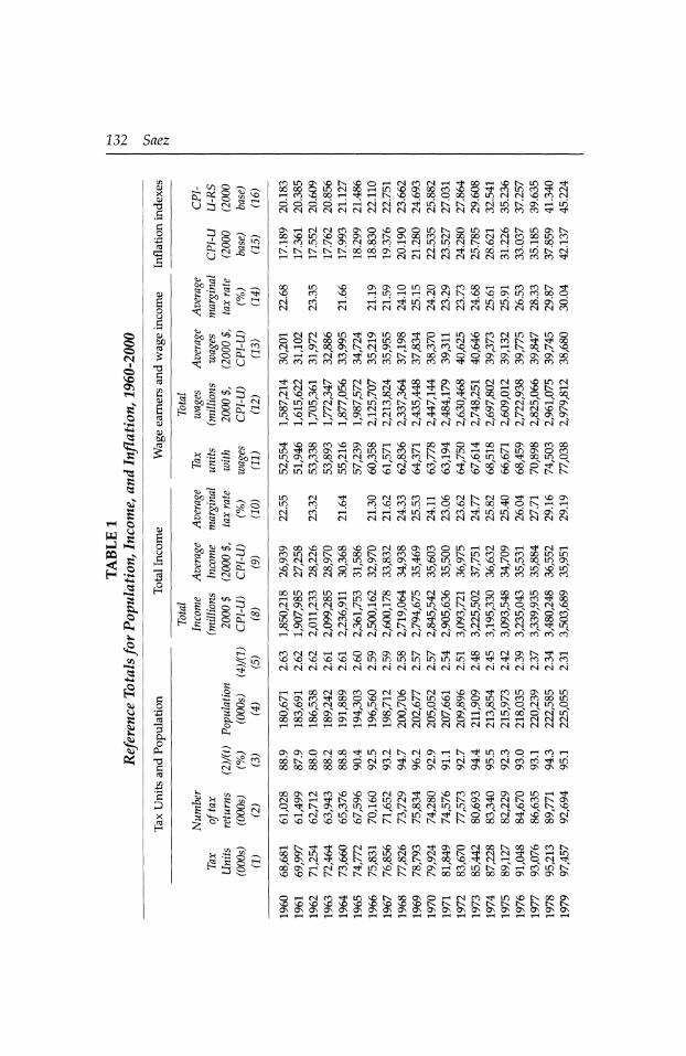
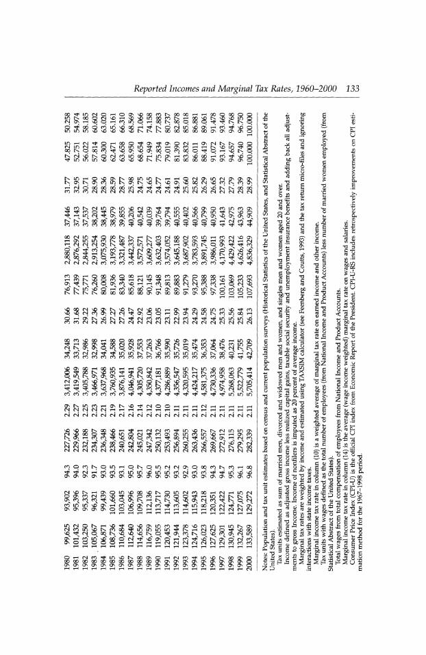
Table 1, since 1960, the average number of individuals per tax unit has
decreased from 2.6 to 2.1 because of the decrease in the average number of dependent children per tax unit as well as the decrease in the fraction of married tax units. Those long-term demographic changes imply that
real average income growth per tax unit will be substantially smaller than
real income growth per capita. These demographic changes can also affect
top income shares if the reduction in tax unit size is not uniform across
income groups. However, the tax return data show that the reduction in tax unit size has been about the same for high-income taxpayers as it has for the U.S. population as a whole. From 1960 to 2000, the number of indi
viduals per tax unit in the top decile has declined from 3.6 to 2.9, which is the same 20 percent decline as in the general population (from 2.6 to 2.1).
From 1960 to 2000, the fraction of married tax units has declined from about 60 to 50 percent for the total population (due to the increased num
ber of single parents and unmarried couples) but only from 90 to 85 per cent for the top decile tax units. An increase in single tax units with lower incomes contributes to increasing top income shares. Similarly, an
increase in the correlation of earnings between spouses (due, for example, to the increased labor force participation of married women) would also increase top income shares estimated at the tax unit level. Those slow
moving demographic changes are small, however, relative to the dramatic trends I document and can explain at best only a small fraction of the
changes in the top most income shares. Each upper-income group is defined relative to the total number of
potential tax units in the entire U.S. population, estimated from popula tion and family census data as the sum of married men, divorced and
widowed men and women, and single adults never married (age 20 and
There is no micro data for years 1961,1963, and 1965.
23 The main (and very minor) difference is that government transfers such as social security benefits and unemployment compensation have been excluded from the income definition in this paper to obtain better consistency in the income definition over the years. The esti
mates have been extended to year 2000.
132 Saez
? c
? T3
CU
i co O ~N t-i ev O ^ ?h ?? O ? U ?3 CU ?
3? ? 2 Ci ?
fi t* s
S I ? ? "
*-. ? Q ^^ ^3 -~s
rO CS ?- O p1 H 0 S (N U
0 g ^
^o e "?2 ̂ ~.
If 2 g g
B te O i ?.
S ?8?^ ^ ^ rsi U
S .2 o ^V O ?2 O ni,
> ^ C2
Il ?SS 5 ^"? S
? ? s C
H^Xny?NifiO't "
in m n vu en m GOOOOinCNlOOrHLOv?ONOOCO ~ _
ddddHHddcn'?iriiNN^Ni?iNo?Hiri
asT-H(N(NcooNOv?)oomt%oiDT-Hv>oi>%maNi^ oovoinvooNONcnNooofONoOQONNmooinco
HcoiriKocNoocoH^ininrjN^tviOHooH
HMN^in^oinoo^OHin^rtNinNino OONOO^NHinO\CONH(S^NrON^^(X) (S h Onv X ON N N ONs H ? n CO \C \? CO H N 00 N O o h h n rn ri in iri N N ?d On ov n o\v ov mv ?tT n\ on
s cn? co ^ in in N uj uj l^. l^ 00 c> o o
cocncncncncn^^ On On On On On 00 CO CO CO CO CO CO
333 3
T-i<NN?>TtmKoc^ - es vu co cov q in N oo co
N lo in es n nv in cn . '
_. oohonnoonhcoco in vu N N CO o\ H CN co ^v H H H H H H ri (N o? CN CN CN CN CN CN CN CN CN CN CN
ONOO^-HCNCNOON?incN tNvOmOT?i CO vD N H
H "tf CN 00v Ov ON CD O 00v i? O 00 KV 0> CN in H On OOCO^OnOCNCNnOK
^v?OOCO^OnOOH^HOO^O^OOHC^OOCOOO in^coa\HcomNcoNNOMnHHMno\oco in o\ co ? cmv n cov in oos co n h n \c in vu ̂ oov in q <n ri ?D rO \0 !*> S ri ri ^f
^ ^ ^ Pi* PS >S ?? P :* ?^ inmininminov?^ O \?) O ^O N N N
s 0(N|COCOrt\?(NNNO^H\?O\ co^coinHq^tsoo^qtNHH
HH^iri^c?co^inin'votso?a! CNCNCNCNCNCNCNCNCNCNCNCNCNCN
(J\00^O00\CO(N00ac0OinH(N0\H'tMrt comNK\oooNcoco^ooNincoocoooinin on cN cN o^ en in on co on ^s ^ in on n vo n in oo in o\
^ nv x od oN h es co1 ̂ s in in in ^s n vd ̂ in in vov in CNCNCNCNCOCOCOCOCOCOCOCOCOCOCOCOCOCOCOCO
oomcoiOHcocN!oo^incNi^H(Niooocoinooa\ HOOCOOOHin\?)N\ON^COCN|OcO?,'?CO'?OO cN on cm cn o\s n h h q o in o n in cov in q ov f| vo
d" kv h on vo rHoooN^inincoinincovinoNOco _ . . . ?^ w^oooN^ioiocoinmcoino\oco inO*-lONCOvsOOOT?ion^ooncnononcocoooo ??s ?i. R R ^t ^ ^ ^v Ns Nv ??v ?l ?v ^1 Hv R ^1 ^ 't ^ H H CN Cn? CN CN CN CN N CN CN CN co' COS CO W COV CO CO ?
COC^(N|HHOO>OOONN'<?HOOinCN|ON^H ^vov?vo^^inininininininii^^cocococo cncncnHcncncncncnHHcnHcncncnHHcncn
HHOOtSO\COO(N^)NNH^O\ NOACOtMO^HOMCvOOsO-. . ......--. vONOincNoocoinr^tNNOON.ooooNoooNOcNino
OCOn.OOnt-I'^n.DOO OOOOOOXOnOnOnONwwww?-,. HHHHHHHHCN|fN!CN|rJNCN!(N|(N|(N|
cNiniNONT-HcomooocN PPPPrlr-irlrl^CN
m - . CN CN CN
o\0\ocNioo^mcN!NcMOHN'<tincoqHcoH CCNo?XO?OCNCO^^CNHCN^lriNc?cO^in OOOOOOOOOOOnOnOnONOnOnOnOnOnOnOnOnONOnOn
OOONCNCON?N?)OCNONT}HOvDCOCOOONOinrH^ CN|0\H^NO\?in^C000NN0\^CNNC0NON
q ^v N o\v co in h \ov N oo n in in ^v cov f\{ ̂ ^ n vo r-? r-i cN co in in os h cov in ^v ^v kv o co cN ̂ v vd" on cn \?\OvO^^\CNNKNNNK0000000000Q0O\
rH IN t^ r* 00 On m v? ^3 On CN ri
CN r-l VO VO CO tF _ IN CO m CN ON CN vO IN 00v 00v 00v IN On
oo* on* r-T cn cov ̂V in no in oov on x-f co* in in' on' h co* in IN vO^NNNKNNNNKOOOOMOOOOOnOnOnOn
ONOCNOOlNOOvOCOlN "N^CNlN^NHin vO^CNrHOOCN??*
OnOnOnOnOnOnOnOnOnOnOnOnOnOnOnOnOnOnOnOn
Reported Incomes and Marginal Tax Rates, 1960-2000 133
00 tF in in CN On
mcNOrHOONNOOOCOtNOOOOrHT-iOOOOOOO "~N^H\?vcir)oocoNHoo\ON^^mo ?
HCOIOOHOONOOOOOO^TfiNNO 2 s T?? 00* ? m m vo
inT-HCN^OrHOOO^ON^ONOCNT-HONCNlNlNOO NiocNiHONininmrfcoHONcoHHNvoin'?o ooiNpoqco^NOONN?cjNoqpcooqp^prHN?iNjp
NCNi^Ndc?co^o?HLno?Hc?^o?Hco^vod ^iniOin^^^^^KNN?OQOOOOOONONONONO
HNO00000000inr?(r?rfi(^inin\uv0NN0000 COCOCOCNCNCNCNCNCNCNCNCNCNCNCNCNCNCNCNCNCN
vocoiNcNinoNinvocNON^'tincM coo^Nino^co^ONin ONOocNinoiNiNin IN IN IN 00 00 00* CO CO CO CO CO CO s?
' ?" On On ^ CO CO
- , NO On O CO m CO On ON.D0Ninr}H|NN?)O ^ in N ON vO ON O; 0>v ?* O CD O rH CN CO**
Ttj"
OONtnr(*OOONNHNcO HONinmcoNoocoNNo rH CN CN CN On IN rtf CO LO CN "tf 3 \0 -f CO in CO** H CN CN ON CN T>^ ?*hNONCS^NOCO
CNOOCNCOinHCOCN|^>0\ moOOON'?HONCNlHCNl moOOON^HONCNlHCN)' q h on in in ov on ^ ^ cov .*, -v, v, ?, K-j ,? v>, ,.>, w^ vV "tf LO IN CO rH NO* O On no vu
3;N-*HN0NCN^NOC0N^00000N00N(NfNC0 oo oo oo on q h co ̂ in vq ̂ in \o ^ n oov on h ^ vo oo CN CN CN CN COV CO COV CO COV COV COV CO COV CO COV CO CO rji rfi hh~ "*
OOHinoOCOCOONO _. ~. _^ -u - oo IN IN 00 rH On CO CO CO NO NO CO ON
PJ (?TN r-i <w> uu ^J i-J uu r-i U) uu oj cj un <?_; i*j uu r?i un cj itJ rHCOlNNOQC0^rHCNTf"^r-H00lNlN00CONONOCOON ON ̂ N CN ? On CO vOs rH h COv 00v 00v CN CN CO CO H O CN NOv
^ N in NC d h co in oov d h on on h co" in n d co in n1 INKInINOOOOOOOOOOOnOnOOOOOnOnOnOnOOOO rH r-i rH rH
NOOOCNNOONlNNOlNCNNOinrHON'^ONOOincONO'HHCO ^NOCNCOONCNCN^ONOprHONOSCNLniNCOinoqrH OrHO?iNvoKiN^cNcocdcocNco^^^LnininNO COCOCNCNCNCNCNCNCNCNCNCNCNCNCNCNCNCNCNCNCN
OOCONOOOrHOOOOOCOCONOONOONTtCO^NOrHinON ^HOOON^OOCNlCNin^N?ONCNlHKinvONCOinO
(NNONONOinOONinCNlMnNOrJicOO^CNNN
SI 'S
NOONOOrHOOmrHrHOCNrHONtNintNinNOOOCOON'stf ?^00N\i)CO^^fNin<0000tONHNcOin^NH v in in onv onv on rH onv t^ oov rH oov in in cn cov cov onv ov tN.v ^v CN ON* in NO* IN ?* NO** vO in O IN NO* VO ? ?tf rH ?* "^f GO* cn in HHO^CONON-?OlOKOOinN-.
' . - _ . ~
rJ^T^H^r^vOvINOOpcOCOtOCNCOCO CO CO CO** CO CO CO CO "?* rj?* t^h* tJ?" t# ?tf -^
OO CO IN no CN O in N ON cn in N r? rti ^s in in in
iNVOTfCNOOrHrHrHCNrHrHrHrHrH
CNrNJCNCNCNCNCNCNC\?HHcs?HcNHcNCNCNCNCNCN
m on On CO CN CO
IN ON
COOCOlNOinrHplNpinCNCNONpoqcOlNCOrHOq H^Hhf\J^rnrnrnLnin'\?inincOcNCOCO^ ONOnOnOnOnOnOnOnOnOnOnOnOnOn On On On On On On On
CN NO tN rH ON O ON CO CS
* ON CO CO CO
_ o m vo oo no CO NO "^ ON O CO r-i
^ NO O ON IN rH IN tNOinCNCOOOrHCNrHinCN
HCOOO^HinCNlNNN INnOnOOnCNCO^INOCN
comm^ONHco^ONCNco^co^inooocN^NON ONONONONONOOOOrHrHrHrHrHrHrHCNCNCNCNCN
incNoiNrHNO^ONOONinco^ooNocoinrHLniNON cNjcoin^Ncooofinminm^NHCNcNo^vooo vOv r* CN Ov Xv IN NOv NO vO IN CD -^ On^ COv ?N O^ NO COv ON CN in
ON* rH CO** in NO** 00V O* CN "^ NO* ON O rH CO* "tf ^O* IN ON O CN CO** ONOOOOOrHrHrHTHrHCNCNCNCNlCNCNCNCOCOCO
O rH CN 00 CO CO - On On ON On On On On On On On
_ O rH CN CO 95 &&&& ^h in no IN 00 On O ON On ON On On On O ON On On On On On O rH rH rH rH rH rH CN
X -afr
-gss-s
-M KT, ̂ Si ?S
llifl H Cfl u > O .
S B
O) > i?i > * * Pi o <u U
i S8S| ! s -s ft il 8?^k
nJ QJ >H - a
O id
3 v
?^ ? +J .t? r^3
S g o .S I ? 3 ffl
oj .a ?h wd^h a? ' R3 CTJ rj -h bo? - ..
c
C/?
134 Saez
above).24 The income definition I use is consistent over time and includes
all income items except realized capital gains reported on tax returns and
before all deductions such as adjustments to gross income, exemptions, and itemized and standard deductions.251 exclude government transfers
such as social security (SS) benefits and unemployment insurance (UI) benefits. Thus, my income measure is defined as adjusted gross income
(AGI) less realized capital gains included in AGI, less taxable SS and UI
benefits, plus all the adjustments to gross income. Hence, my measure of
income is a broader measure than taxable income, on which many previ ous studies have focused.
If deductions to income, such as charitable giving, mortgage interest
payments, etc., are also responsive to taxation, taxable income might be more responsive to tax rates than my broader income measure. Because
the nature of deductions allowed has changed substantially over the
period 1960-2000, however, it is impossible to construct a consistent tax
able income definition over the full period. As a result, refer to previous studies analyzing specifically the components of taxable income that I
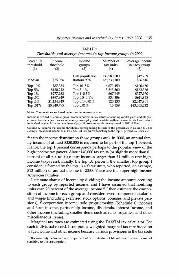
exclude from the analysis. As in Piketty and Saez (2003), I consider various groups within the top
decile of the income distribution. To get a more concrete sense of those
upper-income groups, Table 2 displays the thresholds, the average income
level in each group, and the number of tax units in each group, all for
2000. The median income as well as the average income for the bottom 90
percent of tax units, are quite low, around $25,000. Those numbers are
smaller than those reported by the Census Bureau based on the Current
Population Survey (CPS) for two reasons. First, my income definition
does not include any government transfers. Second, CPS income is
reported at the household level, which is a larger unit than the tax unit I
consider.26
The groups in the top decile below the top 1 percent (the top 10-5 per cent denotes the bottom half of the top decile, and the top 5-1 percent denotes the next four percentiles) have average incomes of $100,000 and
$160,000, respectively, which corresponds to the popular view of the middle
income and upper-middle-income class (perhaps surprisingly given how
24 From 1960 to 2000, between 90 and 95 percent of potential tax units actually filed an
income tax return because many nontaxable families file to get tax refunds.
25 Realized capital gains are excluded because they form a volatile component of income
and face in general a different tax treatment than do other forms of income. Much of the lit
erature focuses on the response of capital gains realizations to tax changes. See Auerbach
(1988) for a survey. 26 For example, a cohabiting couple or two roommates form a single household but are two
separate taxpayers.
Reported Incomes and Marginal Tax Rates, 1960-2000 135
TABLE 2 Thresholds and average incomes in top income groups in 2000
Percentile
threshold
(1)
Income
threshold
(2)
Income
groups
(3)
Number of
tax units
(4)
Average income
in each group (5)
Median
Top 10%
Top 5%
Top 1%
Top .5%
Top .1%
Top .01%
$25,076
$87,334 $120,212 $277,983 $397,949
$1,134,849 $5,349,795
Full population Bottom 90%
Top 10-5%
Top 5-1%
Top 1-0.5%
Top 0.5-0.1%
Top 0.1-0.01%
Top 0.01%
133,589,000 120,230,100
6,679,450 5,343,560
667,945 534,356 120,230
13,359
$42,709 $26,616
$100,480 $162,366 $327,970 $611,848
$2,047,801 $13,055,242
Notes: Computations are based on income tax return statistics.
Income is defined as annual gross income reported on tax returns excluding capital gains and all gov ernment transfers (such as social security, unemployment benefits, welfare payments, etc.) and before individual income taxes and employees' payroll taxes. Amounts are expressed in 2000 dollars.
Column (2) reports the income thresholds corresponding to each of the percentiles in column (1). For
example, an annual income of at least $87,334 is required to belong to the top 10 percent tax units, etc.
far up the income distribution those groups are). In 2000, an annual fam
ily income of at least $280,000 is required to be part of the top 1 percent. Hence, the top 1 percent corresponds perhaps to the popular view of the
high-income tax payers. About 140,000 tax units (or slightly more than 0.1
percent of all tax units) report incomes larger than $1 million (the high income taxpayers). Finally, the top .01 percent, the smallest top group I
consider, is formed by the top 13,400 tax units, who reported, on average, $13 million of annual income in 2000. These are the super-high-income
American families. I estimate shares of income by dividing the income amounts accruing
to each group by reported income, and I have assumed that nonfiling units earn 20 percent of the average income.271 then estimate the compo sition of income for each group and consider seven components: salaries
and wages (including exercised stock options, bonuses, and private pen sions), S-corporation income, sole proprietorship (Schedule C income) and farm income, partnership income, dividends, interest income, and
other income (including smaller items such as rents, royalties, and other
miscellaneous items).
Marginal tax rates are estimated using the TAXSIM tax calculator. For
each individual record, I compute a weighted marginal tax rate based on
wage income and other income because various provisions in the tax code
27 Because only between 5 and 10 percent of tax units do not file returns, my results are not
sensitive to this assumption.
236 Saez
generate differences in the tax treatment of wage income and other forms of income. For each income group, I then estimate an average marginal tax rate weighted by income.28 Note that my marginal tax rate computa tions ignore state income taxes because the data does not provide state
information for high-income earners. My tax measure also ignores other
taxes such as social security and Medicare taxes, corporate taxes, and non
income taxes such as sales and excise taxes.
I use the same methodology to compute top wage shares using wages and salaries reported on tax returns. Wages and salaries include exercised
stock options and bonuses. In this case, groups are defined relative to the
total number of tax units, with positive wage income estimated as the
number of part-time and full-time workers from the National Income and
Product Accounts less the number of married women who are employees. The sum of total wages in the economy used to compute shares is
obtained from the National Income and Product Accounts (total compen sation of employees). The marginal tax rates for upper-wage-income
groups are, of course, those relevant for wages and salaries and are also
weighted by wage income (see Table 1). I propose a simple time-series regression methodology to obtain vari
ous elasticity estimates, and illustrate some of the identification difficul
ties. Because of potential heterogeneity in elasticities across income
groups, all regressions are run for a single income group. The simplest
specification consists in regressing log real incomes on log net-of-tax rates
(and a constant) for a given group. Of course, as real incomes grow over
time, time trends can be added in the regression to control for exogenous (i.e., non-tax-related) real income growth. These estimates are unbiased
estimates of behavioral elasticities if, absent any tax change, real incomes
in that specific group do not change (first specification) or follow a regu lar time pattern (second specification). These assumptions may not be
met. Because many years of data are included, these estimates capture
mostly the long-term behavioral elasticities.29 As we will see, the pattern of average incomes for the full population does not appear to be related
to the evolution of average marginal tax rates. Therefore, to control for
average income growth, most of the regressions are run in terms of log income shares instead of log average incomes.30 These regressions control
28 As we saw above, for tax policy analysis, it is necessary to weight marginal tax rates by income.
29 I leave for future research the regression analysis of the dynamics of tax responses. Such
a formal analysis has been attempted in the case of capital gains realizations. See, for exam
ple, Auerbach (1988).
30 Slemrod (1996) adopted the same approach, although he controlled for nontax factors
explicitly rather than using general time trends controls, as I do here.
Reported Incomes and Marginal Tax Rates, 1960-2000 137
automatically for overall income growth. Adding time trends in that case
amounts to assuming that incomes for the particular group considered
may diverge from the average income in the economy. Because time
series regressions are run and the error terms appear to be correlated over
time (according to the standard Durbin-Watson test), Ordinary Least
Squares (OLS) standard errors are not correct. Therefore, the Newey-West standard errors are computed, assuming that the error terms can be cor
related up to an eight-year lag.31 Because of the progressive structure of the income tax, increases in
incomes lead to higher marginal tax rates, or bracket creep. As a result, an
increase in top income shares (for non-tax-related reasons) might also induce a mechanical increase in the marginal tax rate faced by those high-income
taxpayers, hence potentially biasing downward the elasticity estimates.
A simple way to investigate the extent of the problem is to use the statutory
top marginal income tax rate (or more precisely, the log of 1 minus the top rate) as an instrument for the effective log net-of-tax-rate variable. The
results show that the OLS and Instrumental Variables (IV) estimates are
extremely close, suggesting that progressive structure of the income tax sys tem and bracket creep do not create a significant estimation problem.
3. INCOME SHARES AND MARGINAL TAX RATES
3.1 Trends in Average Incomes
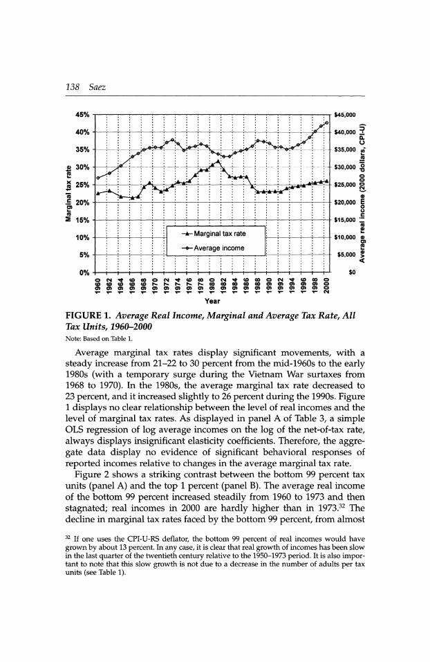
Figure 1 shows the average federal marginal individual income tax rate
(weighted by income) and the average income (per tax unit) reported in
real terms for the full population from 1960 to 2000. Incomes are
expressed in 2000 dollars using the standard Consumer Price Index-All
Urban Consumers (CPI-U) deflator (see Table 1). Figure 1 also shows that
real incomes increased quickly from 1960 to 1973 and then increased
hardly at all until the early 1990s. From 1993 to 2000, real incomes have
increased quickly but are only 13 percent higher than in 1973. Real growth
depends critically on the Consumer Price Index (?PI) deflator.
Improvements in the CPI estimation have been made over the years, and some of them have been incorporated retrospectively in the so-called
Consumer Price Index Research Series using current methods (CPI-U-RS) deflator (see Stewart and Reed, 1999). Using the CPI-U-RS instead of the CPI-U would display about 29 percent real income growth instead of 13
percent from 1973 to 2000 (see Table 1).
31 An eight-year lag is close to maximizing the size of the standard errors and thus should
be seen as conservative.
138 Saez
45% $45,000
OCMtCOCOOCM^COCOOCMtCOCOOCM^tttOOO (0(0(DCD(0SSSSS00000000000)0)0)Cf)CDO
0)0)0)0)0)0)0)0)0)0)0)90)0)0)0)0)0)0)0)0
Year
FIGURE 1. Average Real Income, Marginal and Average Tax Rate, All
Tax Units, 1960-2000
Note: Based on Table 1.
Average marginal tax rates display significant movements, with a
steady increase from 21-22 to 30 percent from the mid-1960s to the early 1980s (with a temporary surge during the Vietnam War surtaxes from
1968 to 1970). In the 1980s, the average marginal tax rate decreased to
23 percent, and it increased slightly to 26 percent during the 1990s. Figure 1 displays no clear relationship between the level of real incomes and the
level of marginal tax rates. As displayed in panel A of Table 3, a simple OLS regression of log average incomes on the log of the net-of-tax rate,
always displays insignificant elasticity coefficients. Therefore, the aggre
gate data display no evidence of significant behavioral responses of
reported incomes relative to changes in the average marginal tax rate.
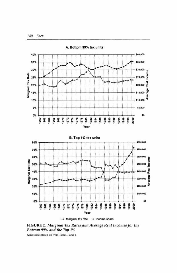
Figure 2 shows a striking contrast between the bottom 99 percent tax
units (panel A) and the top 1 percent (panel B). The average real income
of the bottom 99 percent increased steadily from 1960 to 1973 and then
stagnated; real incomes in 2000 are hardly higher than in 1973.32 The
decline in marginal tax rates faced by the bottom 99 percent, from almost
32 If one uses the CPI-U-RS deflator, the bottom 99 percent of real incomes would have
grown by about 13 percent. In any case, it is clear that real growth of incomes has been slow
in the last quarter of the twentieth century relative to the 1950-1973 period. It is also impor tant to note that this slow growth is not due to a decrease in the number of adults per tax
units (see Table 1).
Reported Incomes and Marginal Tax Rates, 1960-2000 139
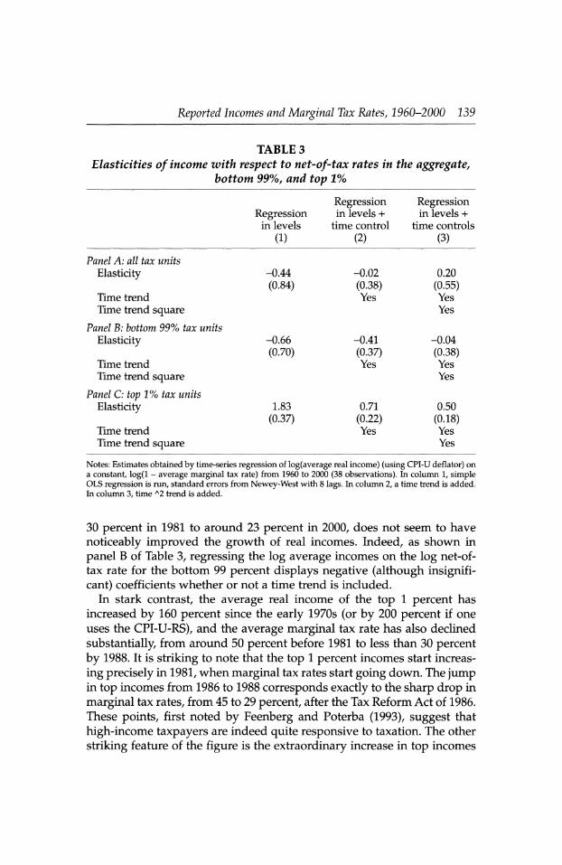
TABLE 3 Elasticities of income with respect to net-of-tax rates in the aggregate,
bottom 99%, and top 1%
Regression in levels
(i)
Regression in levels +
time control
(2)
Regression in levels +
time controls
(3) Panel A: all tax units
Elasticity
Time trend Time trend square
Panel B: bottom 99% tax units
Elasticity
Time trend Time trend square
Panel C: top 1% tax units
Elasticity
Time trend Time trend square
-0.44
(0.84)
-0.66
(0.70)
1.83
(0.37)
-0.02
(0.38) Yes
-0.41
(0.37) Yes
0.71
(0.22) Yes
0.20
(0.55) Yes
Yes
-0.04
(0.38) Yes
Yes
0.50
(0.18) Yes
Yes
Notes: Estimates obtained by time-series regression of log(average real income) (using CPI-U deflator) on a constant, log(l
- average marginal tax rate) from 1960 to 2000 (38 observations). In column 1, simple
OLS regression is run, standard errors from Newey-West with 8 lags. In column 2, a time trend is added. In column 3, time A2 trend is added.
30 percent in 1981 to around 23 percent in 2000, does not seem to have
noticeably improved the growth of real incomes. Indeed, as shown in
panel B of Table 3, regressing the log average incomes on the log net-of tax rate for the bottom 99 percent displays negative (although insignifi cant) coefficients whether or not a time trend is included.
In stark contrast, the average real income of the top 1 percent has
increased by 160 percent since the early 1970s (or by 200 percent if one
uses the CPI-U-RS), and the average marginal tax rate has also declined
substantially, from around 50 percent before 1981 to less than 30 percent
by 1988. It is striking to note that the top 1 percent incomes start increas
ing precisely in 1981, when marginal tax rates start going down. The jump in top incomes from 1986 to 1988 corresponds exactly to the sharp drop in
marginal tax rates, from 45 to 29 percent, after the Tax Reform Act of 1986.
These points, first noted by Feenberg and Poterba (1993), suggest that
high-income taxpayers are indeed quite responsive to taxation. The other
striking feature of the figure is the extraordinary increase in top incomes
140 Saez
A. Bottom 99% tax units
O CM -^ <0 CO O (O (O ID (O (O N
O) 0) 0) O) O) O
Year
B. Top 1% tax units
Tf to CO O) 0) o>
Year
-a- Marginal tax rate - -
Income share
FIGURE 2. Marginal Tax Rates and Average Real Incomes for the
Bottom 99% and the Top 1% Note: Series Based on from Tables 1 and 4.
Reported Incomes and Marginal Tax Rates, 1960-2000 141
from 1994-2000, in spite of the increase in tax rates, from about 32 percent to almost 40 percent in 1993. Thus, although the marginal tax rates faced
by high-income taxpayers in 2000 are hardly lower than in the mid-1980s
(39 percent instead of 44-45 percent), top incomes are more than twice as
large.
Figure 2 illustrates clearly the difficulty of obtaining convincing esti
mates of the elasticity of reported income with respect to the net-of-tax
rate. It seems obvious that the sharp, and unprecedented, increase in
incomes from 1986 to 1988 is related to the large decrease in marginal tax
rates that happened exactly during those years. The central issue, how
ever, is whether this short-term response persists over time. In particular, how should we interpret the continuing rise in top incomes since 1994? If
one thinks that this surge is evidence of diverging trends between high income taxpayers and the rest of the population independent of tax pol
icy, which started in the 1970s, then it is tempting to consider the response to TRA1986 as a purely short-term spike followed by lower growth from
1988 to 1993, before getting back to the normal upward trend by 1994. On
the other hand, one could argue that the surge in top incomes since the
mid-1990s might have been the long-term consequence of the decrease in tax rates in the 1980s and that such a surge would not have occurred
had tax rates for high-income taxpayers remained as high as they did in
the 1960s and 1970s. I will return to this point later.
These issues are illustrated formally in the regression results in panel C
of Table 3. When no time trend is included in the regression of log income on log net-of-tax rate, all the growth in top incomes is attributed to the decline in top rates, and the elasticity obtained is extremely large 1.83
(.37). In contrast, including a time trend produces a much smaller,
although still sizable, elasticity of .71 (.22) because part of the rise in top incomes is attributed to a secular rise. Adding an additional time square control further reduces the elasticity to 0.5 (0.18).
This analysis also shows that comparing two single years by taking the ratio of the difference in log incomes to the difference in log net-of tax
rates, as is done in most studies, can produce a wide range of elasticity estimates. Comparing 1981 to 1984, as in Lindsey (1987), produces an elas
ticity of 0.77.33 Comparing 1985 and 1988, as in Feldstein (1995) and Auten
and Carroll (1999), produces an extremely large 1.7 elasticity.34 In contrast,
33 Lindsey (1987) obtains larger estimates because he compares the upper-income to the
middle-income groups, creating an upward bias if, as is apparent in the data, elasticities are
increasing with income (see discussion in section 2.1). 34
Auten and Carroll (1999) obtain a much smaller 0.6 elasticity because they compare 1985 to 1989 (instead of 1988, as did Feldstein [1995]) and because of the mean reversion issue dis cussed in Section 2.1, which is difficult to correct with only two years of data.
242 Saez
comparing 1991 to 1994 (as in Goolsbee, 2000b) produces a zero elasticity because top incomes are about constant, while tax rates increase by almost
10 percentage points.35 The elasticity would even become negative if one
compares 1991 to the late 1990s because both top incomes and the tax rate
have increased.36 The large micro data sets can be used to obtain these
simple elasticity estimates directly from regressions at the individual
level, as is done in many studies, with small standard errors. The regres sion counterpart would be to pool the samples of top 1 percent earners for
the pre- and postreform years and run a Two Stage Least Squares (2SLS)
regression of log incomes on the log net-of-tax rate using as an instrument a postyear dummy.37 To cast additional light on these issues and try to
separate tax effects from other effects, I turn to a closer analysis of various
upper-income groups, with particular emphasis on the change in the com
position of reported incomes.
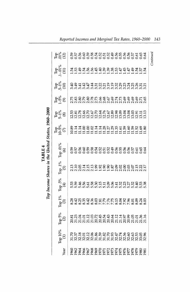
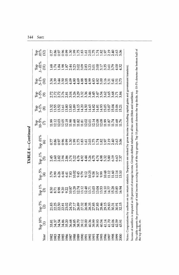
3.2 Trends in Top Income Shares and Marginal Tax Rates
Average real incomes do not seem to respond to average marginal tax
rates in the aggregate, and responses seem to be concentrated in the upper 1 percent of the income distribution. From now on, therefore, top incomes are normalized by considering the shares of total income accruing to var
ious upper-income groups (as in Feenberg and Poterba, 1993, 2000, and
Piketty and Saez, 2003). This approach has two advantages. First, the
income share measures are independent of the CPI deflator used. Second, the top shares are normalized automatically for overall real and nominal
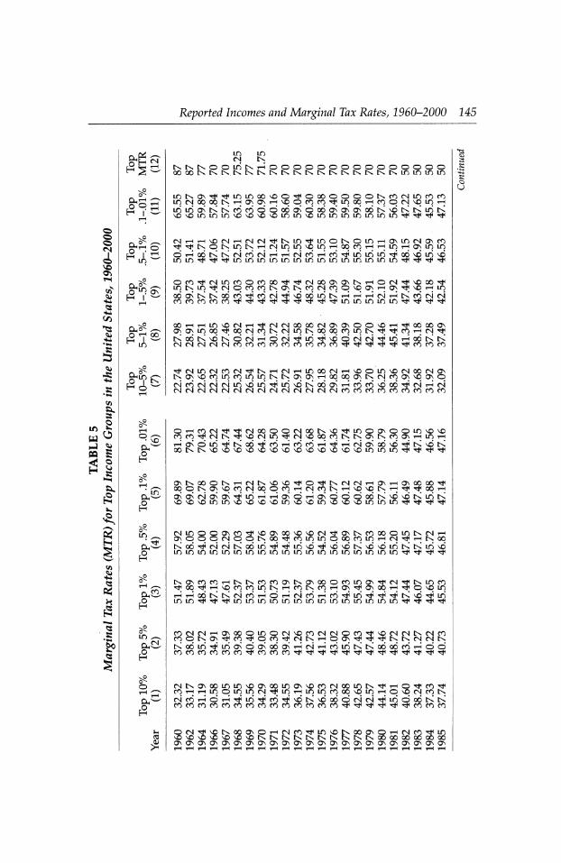
growth in incomes. All the top income share series and corresponding average marginal tax rates (income weighted) are reported in Tables 4
and 5, respectively. Table 6 displays several regressions of the (log) top 1 percent income
share on the log net-of-tax rate, varying the number of time trend controls
and instrumenting or not the tax variable with the log net-of-tax top rate. As discussed above, introducing time trends reduces substantially the elasticity, from 1.6 (with no controls) to about 0.6-0.7 (with many
controls). After adding linear and square controls in time, the adjusted 35 In contrast, comparing 1992 to 1993 would produce a significant short-term elasticity of
0.63, as in Feldstein and Feenberg (1996).
36 Carroll (1998) and Sammartino and Wiener (1997) analyze panel tax return data. They also
show that short-term responses around OBRA 1992 are much larger than longer-term responses.
37 It is doubtful, however, that these small standard errors would be accurate because ran
dom year effects are most likely to be present in the data, making 2SLS standard errors far
too low and hence worthless (in addition to creating the identification problems discussed
in section 2.1). See Bertrand, Duflo, and Mullainathan (2003) for a detailed discussion of
these econometric issues.
Reported Incomes and Marginal Tax Rates, 1960-2000 143
9i
C/}
^ -IS
S?
o
a.
e2
?-2 H o O
r-1 m ^
r
r
Oh
e2
0-^
(0
2
C7NK\DOONOO^(NH(NO\vOlO^)vOI\Hir}rlH Loii^u^^iOLoinLOLoiT?TtHinir?LoiOLnvovo^o
?????????????????O?
Oa\HMN^HCNHOM^(NONCO^mvOHH rrJT^^|H^TJHT^cO(NCNrH^H CO CN CN CN CN CN CO CNJ foc?c?c?coc?c?cocncocof?c?cocncocnc?c?
LOCOOONOOOfOvOOONON^fOOMjNOMJiHl?i r^oqoqrvjoqrvj^Vsp^^^irsjr^v?vov?^i^.^ CNCNCNCNCNCNCNCNCNCNCNCNCNCNCNCNCNCNCN
lOoqts^Nvqtsv?iN^oqoNqooqoNHH HHdHtN?HHNHH(N(Nrnr?fOcriHfOcn
ON^^OOtN^^OONOMOHONO^fNONO MHHOOOHH(N(N(Scn^oio^inm^oo
ONNOOONOO^NHCNaw?lO^v?NHlf)^
??o????d?????????cJC)
COOlf)^infOa\(NOONO(NOfOMO(NN rH^OrH^rHONONONCTNOqOOOOOrHCNT?I CN'HcNHcNCNrHrHrHrHrHCNCNCNCNCNCNCNCN
COO\v?\?HOOOinHON\?>H(NfriN(NOcOOO inLo^iovoincoHTHoo^cncNrico^Loco lOini?SLoinirii?SuSi^LnirJLni^iiSiniOLOLo
(N^NCO^COqoqNNNHOO\ONOO(NO o6o6o?o?o6o6o?Kr>!KKo?o?KKcx5o6o?cx5
HcO'*HMcoMiri^cO'f(N^NaNinH\o\?i oqrjqqrHqiN^i^^^HHONONqqcOH
OrHrH^rH^OOOOO^rHOOrHrHrHT-H CNCNCNCNCNCNCNCNCNCNCNCNCNCNCNCNCNCNCN
ONooH^^^ONrJOroN^^ororoin^ NcnHqHqoqir)oqNo\^NLOv?\qLqqa\ rHCNCNCNCNCNrHrHT^rHrHCNCNH^HcNCOCN comcncncomcococococococococococncnco
OM^\ONOOO\OH(NCO^ir)VONOOONOH
ONONONONGNCisciNcyNQNGrscy\cyNC^c7NC^cyNON^ON
144 Saez
Ch?^ ̂
3 3?
N\?N^O\OOMDCOHfOlf)^(NNa\OCO^) Noqo\oso\cooNNoqvqqtstsoqo\H^v?q ? ? CD ? ? T-H rH i-H H rH CN t-? t-1 i-H H CN CN CN CO
oo^^ooN^ro(SONfOcnHOMnHO\0(N \?NoqoNoq^(sqqoqr>iqqHeovqNqco
HHHHHfNfocncoHc?rncococoror?^^
"^ON^OLnONOasOOOOaNCOCNO^OrHrHrHCO coco^inii^poqvqoqvooNcx)ooprHcOT|Hifi^ COcricOc?cO^rf^^^^^Ttl?SuSLOLnLOLn
r^^r^iNoopcNcNcoco^^^iTisq^vqiNoq
MiocNHOcooMnooir)(NHroinN^vOH coinin\?oqoqoqH(sjif}\?oqoqa\qqqo(S COCOCOCOCOCOCO^^^rji^^T^LOliSliSir^Ln
ONMmiO000000CSH(NH^xxa\N^00vD ONHqqHo^^oooqqqHoqoNoqts^is
H'ddrJlNHHHHCNN?SHdHHHHH
Cn V4-J y t? G a? 'S 2 ^ bO c rv
TS ̂ 2 43 t? -^
t?
t?
l 3
i
Cm
t2
LO ^
r
e2
e2
(S
2
NvoN^ONOOMncoHfOin^NNONOfoo N(?ONONa\cooNiNoq^qNtsoqa;rH^^q ? ? O ? ? rH rH rH rH t^' CN rH rH rH rH CN CN CN CO
inO(N^^^M^(N^vDir)^oOfN|OONCON ^\OOOONOONNKO\^NNKO\COOOHV?CO
r^ONCN^^oo^^i^rH^LniooN^^^0^^
Sr^^SfsjOO^S^^-l^^PP^^I^^oo^ OCOCNCOCNCOCOCOCO^^LOU-?v?
LO t>, ON CN CN 00 00 00 ON ON
coinoH(NONO\(Nooioi^Ln^LncnHHin OOCNLOOOOKrHOOCOaNCOOOOO^rHOOCOaSrH
HdHHc?^ts^Nvuo?isNodo?o??dri CNCNCNCNCNCNCNCNCNCNCNCNCNCNCNCNCOCOCO
HN^\?OOOlOOMO^O\fO^^O^O\H oqcoinoqNvqoqNHqrtONOsirjHtsqLocjN co^'^^in^o?odoNONOONONOHH'dcNicn
Mc0^ir)V?N000\OHMC0^in\?N00(^O ooooooooxoooooooM^a\a\a\ONONONONO\o OnOnOnOnQsOnGnOnOnOnOnQsGnOnOnOnOnGnO rHrHrHrHrHrHrHrHrHrHrHrHrHrHrHrHrHrHCN
a. t? 2
.t?
.2
? 2
? ? -S
c o 43
c? t? B o O u
Reported Incomes and Marginal Tax Rates, 1960-2000 145
Ch?=! ct
e2?S
CLr_? ̂ n ^1 ?
e2 I c ^ LO
it"? &
ft s
LO CN LO LN LNLNLNOOLOLNrHOOOOOOOOOOOOOO 00 OO IN IN LN LN NNNNNNNNNNNNMOlOlT)
ioNa\^^ininQO^o^oooooooNcn(SincofO intN(X)ooNHa\0\rH\?qt^f0^inoOHcnqr^^if)H LOLoosisiscocoddodosdoooNONa?odts^NisLnts
(MHHV?CNHiNM^MDrfinONOl^HOMOMONCO ^^NoisLniNHf>jir)in\?inHoqfOrHrHinHONLnin OHo6lSlNCN?c?HrHHf\?c?rHC^^LOLOlOTto6^L6^
OCO^CNIi^COOCOOO'^^CNOOONONLNrHOCN^v.OCX)^ inNif)^(NqcocoNONNcoc^coq^ONHON^vOHio 0?ONNlN0?c0^C0H^^0?lf?NHHHdHNcOtN?CN
OOrHrHLO^OCNrHr^cNcNOOOOCNasaNOO^OrHTtOOOOON ONaMnoo^xtNcnNtNinNoooocoinN^H/fOHtN^ NoONvoNoHHON^iri^ycoHd^LnHooisN
CN CN CN CN CN CO CO COCOCOCOCOCOCO^^^TtH^^COCOCO
^CNLnCNCOCN^LNrHCNrHLOOOCNrHV^OLOvOCNOOCNON NO\^ocoir)rtLniDNNa?ONHoqoqoNN(NfOON^a\0
CNCO^CNCNLn^Ln^LO^?L<00^rHCO^\D00^CNrHCN CNCNCNCNCNCNCNCNCNCNCNCNCNCNCOCOCOCOCOCOCOCOCO
eS
Oh S
e9
e2
r
03
2
c^co^cNLN^vqcNLn^cNvooqcoLNbNONLNcoo^ HONOLO^ISO?^fOHC?cOH^HHONod^i'tSVOtS OOLNlNVvO^vO^^^^^^^^^vOLOLOLO^^"^^
0\N00ONH(NN\?)^^O^N(NMHt7\H0N0000't ?oqNa\vo?NoqqcOHNcoNHvov?NH^^oqH ONaNONa?^irJHHadH'oNoddoois^v?isiriis
Minooo\co^\?)a\oo\?vO(N^ONNcooooinNrjH ONOOOtNOONOO^cOininOOOfOlDHN^HNOO LNo?^HcNLNo?Ln^^ii^vd^vdvdKvdvdir?LxLNLn ininioi^u^inLoin^irjinLoioininLninLTiir)^'*^^
NONrocoHNNcncoa\Na\ooofOLna\^(S^Mnco ^oo^H^c^fOLnNHfONcnHi^^a\(X)H^q^LO HHoONNHwHOHNr?Hcn'iinTjiTji^Nv?TjiLn
COCNCNrHC^OOOLOOCNvOCOCNCNOCO^^OCNCNlNCNCO (r)qN(^^co^qcn^NNHqoN^^^Nis(N(NN tsa)ir)^iooNda\o6oNHHHcoLntsNo6o?coHdd cOcOcOcOcOcO^cOcOcO^^r^^^^^^^TfT?HT^T?H
(NNaNOOir)ir)\Da\oOLo<^\?fnMxioN^HO^co^ COrHrHinpii^li^CN^LQrHLOLOCOOO^LnrHOvOCNCOlN fN?c?HdrHTtio^c?^v?^v?o?dfSr]^LridodtsiN CO CO CO CO CO CO CO ( ^^COCOCO
OCN^VOLXOOONOrHCNCO^LO^OtNOOasOrHCNCO^Ljn vu^\DvO^vO\?NNNNNNNNNN000000000000
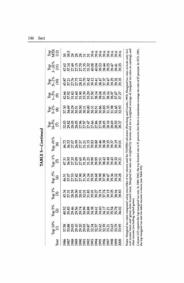
146 Saez
e2sc
E? i ~
I-ge
r
r
CU
CU e2
cd 2
LO vO^O^O^OvOvO^vD OO?oOOOOOHHaONONO?O?O?O?ON
LOCOCNCNCNCOCOCOCOCOCOCOCOCOCO
CN^ONlOOLOCNOOrflCO'^LOLNrHLO VsOrHT^rHLN^COppLq^LO'^'^CO
NNNNNHrnddONO?CJNONONI^ ^COCNCNCNICOCO^^COCOCOCOCOCO
NHV?1T)IOOMMHNNNON(NIO XrNJlNNHN^HrjH^cO^CNCOCO
ioNNNo6rHHONa\o?iso\ONO\o\ rPCOCNCNCNCOCOCOCOCOCOCOCOCOCO
^(NCOOOONONO^^^^NNN vqoNoqvqoNcocNLOrHpcNrHp^qcN
Hnhhhc?cono?o?iso?o?nin ^COCOCOCOCOCOCOCOCOCOCOCOCOCO
OONONrHOrHOrHrHV?icOLOOOLOCO COvOCNLOLOrHOCOLOOOOOCOOs^ON LN^??????O??rHrHCNCN COCOCOCOCOCOCOCOCOCOCOCOCOCOCO
COMlDinvONN^vO^LCOOONCON qoqqqoNLn^vqoqoNOrH^qLoco
cnonoooolnlnlninKlnoooooooooo cocncncncncncncncncncncncncncn
MCONONNHlOCOO'sOOOinNcTNH IN?LOpCTNli^CNrHOqoq^COCOCOrHp v?\?Nv?1NHHOnc7\(3no6onO\(?\On "<tfCOCNCNCNCOCOCOCOCOCOCOCOCOCO
rHCOCOaNLOONlOOsLOrHCNOOCOCNrH COONCOpvOCNCNOsONLO^rJH'H^COCN iNvdtNLNLNrHrHONa?ONOOONONONCJN
r^COCNCNCNCOCOCOCOCOCOCOCOCOCO
rHLNCOCNOO^LOOOOOOLNv?>CNOO inqLn^a\ir)coLqv?ONa\^cococN
^NNtNNHHO?O?o?lSO?ONO?O? ^COCNCNCNCOCOCOCOCOCOCOCOCOCO
^HONOHHCOHN^^iOiO^cO COCOLQLOONpOqpCNLNLNrHpONOq Lntsodo?o?cNrHO\a\o?iso?aNo6o6 rfCOCNCNCNCOCOCOCOCOCOCOCOCOCO
CNLO^v.Or?HONOOOOrHOLNrHTfOOCN LOoq^LqLNo\oqco^vorHCNLqLNp
diooNO?a?dd^^^^ifi?riiovu ^COCNCNCNCOCOCOCOCOCOCOCOCOCO
OOOOcOOOCON^NCNOnhcOOMO LqoqprHCNONoqcoLO^qcocNvqLNON
KcooncKononc^cnHcncncococ?co COCOCNCNCNCNCNCOCOCOCOCOCOCOCO
^LNOOaNOrHCNCO^LOVOLNOOONO ooooooooao\aa\o\ONO\o\o\ONO OnCJnOnOnOnOnOnOnOnOnOnOnOnOnO rHrHrHrHrHrHrHrHrHrHrHrHrHrHCN
^ t?
bO .s ?
* t?
"?:?> c? O)
di nj
O? (S
2 cu ?S t?
3 S
31 O) O)
I * t? ?
I*
? -5 o ff CO CO
O en
CO Xi On H
?s
T3-S.S CU QJ tO 3 S" g g i u O - en c
? .
ai -a t? s "5
bp bo
e-gl ^ o> x
S x ?
'?fs ? ?2 g o ?O" ^ U t?
8-S'S
Z a? o
Q o^
II
o a*
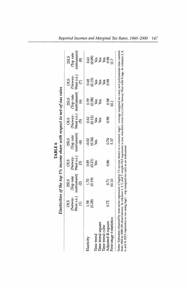
Reported Incomes and Marginal Tax Rates, 1960-2000 147
H
8
o *>
?
?5
hJ ? +j LN 0 0)1/5^
>> oi ?^ g c?^
?? .*-? LO CD c? ^-^
O,
CN? ? r~" c?
>^ ai
OhJ ?^ ̂ co
O? C? ̂ -'
M c?
>>? ai
P) O) c? ̂ -'
?2|
HO\ C? C? C? 00 vO O aj aj aj On LN cd cd ̂ ^ ^ cd rH
00 LO C? C? c? 00 ^q h n; oj ,0) on cd cd <~* ̂ ^ cd
Os 00 c? C? 00 LO O 0) CD ON rH cd cd /* ̂ cd cd
S 2 C? C? ^ <-j ?a> <k O O >< ><
Q O >S I
IOH y) COM aj cd cd ̂
O On LN H
00 00 LO CN
00 ON
LN CO cd LO
00 cd
LN H
C?
g ai
C? U T3 Tj T3 t? C fi C^ P P & 0)
? -h? O) 0)
w ?#!
PPP<;E
s-S
.a cl
? J2

148 Saez
R-square reaches 98 percent, and the elasticity coefficient is not sensitive
to adding additional controls. The IV estimates are close in magnitude to
the OLS estimates and have a strong first stage [except in the case of col umn (4) where the first stage is weak]. This finding suggests that the issue
of reverse causality because of the progressive nature of the tax schedule
is not an important issue. Figure 3 illustrates these issues by plotting,
along with the top 1 percent income share series, the fitted values from the
regressions with no time controls (line with triangles) and with two time
controls (solid line). The line with triangles shows that the pure tax effects
explain quite poorly the evolution of the top 1 percent income share. In con
trast, the solid line with two time trends captures extremely well the pattern of the top 1 percent income share (the adjusted R-square of the regression is 98 percent). The line with squares in Figure 3 displays the counterfac
tual pattern, assuming that the marginal tax rate for the top 1 percent had
remained constant since 1960. This curve shows that most of the growth in the top 1 percent income share is due to the time trends and that only two out of the nine-percentage-point increase in the top 1 percent income
OWt(OOOON^(i)OOOWTf(?COOW^tOCOO <0<O<O<O<ONNh?l^h-OOOOCOOOOOO)O>O>O>O>O
O>O>0>O>0>O>O>O>O)O)O)O)0>O>O>0)O)0>O>O>O !-T-T-Y-T-!-!-!-T-f-r-1-T-T-T-Y-T-1-l-T-<M
Year
FIGURE 3. The Top 1% Income Share and Titted Values from Elasticity
Regressions Source: Series based on regression analysis presented in Table 6, columns (1) and (5).
Notes: The diamond line is the top 1 percent income share. The line with triangles is the fitted regression curve, including only the net-of-tax rate. The solid line is the fitted regression curve, including time controls. The line with squares is the same fitted regression curve but the marginal tax rate is frozen at the 1960 value.
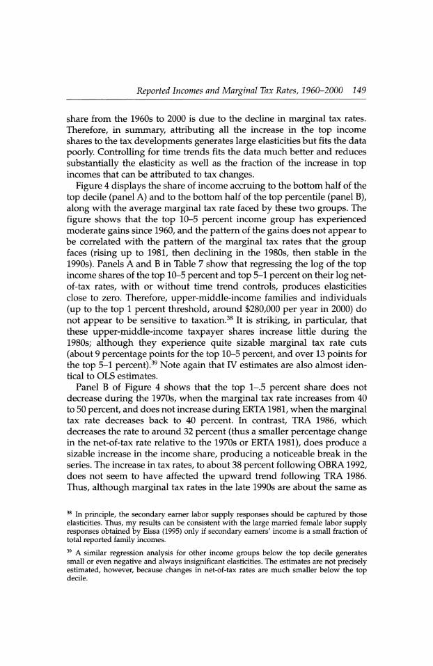
Reported Incomes and Marginal Tax Rates, 1960-2000 149
share from the 1960s to 2000 is due to the decline in marginal tax rates.
Therefore, in summary, attributing all the increase in the top income
shares to the tax developments generates large elasticities but fits the data
poorly. Controlling for time trends fits the data much better and reduces
substantially the elasticity as well as the fraction of the increase in top incomes that can be attributed to tax changes.
Figure 4 displays the share of income accruing to the bottom half of the
top decile (panel A) and to the bottom half of the top percentile (panel B),
along with the average marginal tax rate faced by these two groups. The
figure shows that the top 10-5 percent income group has experienced moderate gains since 1960, and the pattern of the gains does not appear to
be correlated with the pattern of the marginal tax rates that the group faces (rising up to 1981, then declining in the 1980s, then stable in the
1990s). Panels A and B in Table 7 show that regressing the log of the top income shares of the top 10-5 percent and top 5-1 percent on their log net
of-tax rates, with or without time trend controls, produces elasticities
close to zero. Therefore, upper-middle-income families and individuals
(up to the top 1 percent threshold, around $280,000 per year in 2000) do
not appear to be sensitive to taxation.38 It is striking, in particular, that
these upper-middle-income taxpayer shares increase little during the
1980s; although they experience quite sizable marginal tax rate cuts
(about 9 percentage points for the top 10-5 percent, and over 13 points for
the top 5-1 percent).39 Note again that IV estimates are also almost iden
tical to OLS estimates.
Panel B of Figure 4 shows that the top 1-.5 percent share does not
decrease during the 1970s, when the marginal tax rate increases from 40
to 50 percent, and does not increase during ERTA1981, when the marginal tax rate decreases back to 40 percent. In contrast, TRA 1986, which
decreases the rate to around 32 percent (thus a smaller percentage change in the net-of-tax rate relative to the 1970s or ERTA 1981), does produce a
sizable increase in the income share, producing a noticeable break in the
series. The increase in tax rates, to about 38 percent following OBRA 1992, does not seem to have affected the upward trend following TRA 1986.
Thus, although marginal tax rates in the late 1990s are about the same as
38 In principle, the secondary earner labor supply responses should be captured by those
elasticities. Thus, my results can be consistent with the large married female labor supply responses obtained by Eissa (1995) only if secondary earners' income is a small fraction of
total reported family incomes.
39 A similar regression analysis for other income groups below the top decile generates small or even negative and always insignificant elasticities. The estimates are not precisely estimated, however, because changes in net-of-tax rates are much smaller below the top decile.
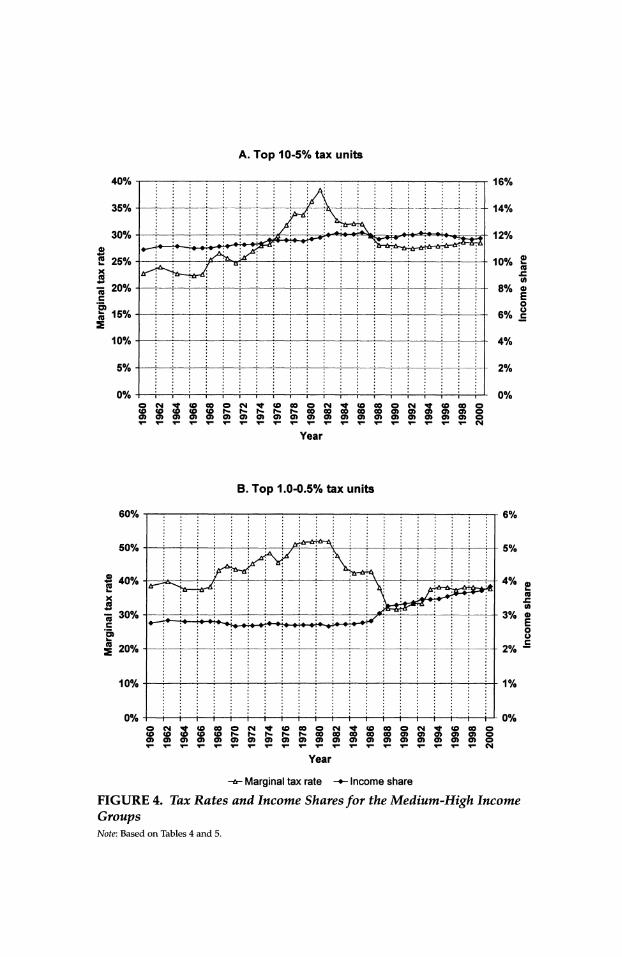
A. Top 10-5% tax units
40% 16%
35% 14%
30%
2 2 25% x
? 20% c US' 15%
- :> ?r+^ 12%
10% g cu JO to 8% ?
6% ? 10% 4%
5% 2%
0% OOI^<0COOCM<*<0OOOCN^><0COOCM<*<0OOO (O(0<6(O(ONSNNN(OeOCOCOeoe)O)(AO)O)O 0)O)0)O)O)O>O)O)0)0)0>O>O)O)0)0>O>0>O)O)O
Year
B. Top 1.0-0.5% tax units
0%
0% -I?i?i?i?i?i?i?i?i?i?i?i???i?i?i?i?i?i?i?M- 0% OtN'$<0OOOM<*<OCOOCN^><0OOOCM<<*<0COO (0(OU(D<ONNNNNcoeoooeoeoo>ao)0)ao 0>0>0>00>0>0>0>0>0>0>0)CDO>0)0)0>0>0>0)0 T-T-T-T-*-T-T-T-Y-T-T-*-T-*-*-*-1-T-T-^tN
Year
-*- Marginal tax rate
- - Income share
FIGURE 4. Tax Rates and Income Shares for the Medium-High Income
Groups Note: Based on Tables 4 and 5.
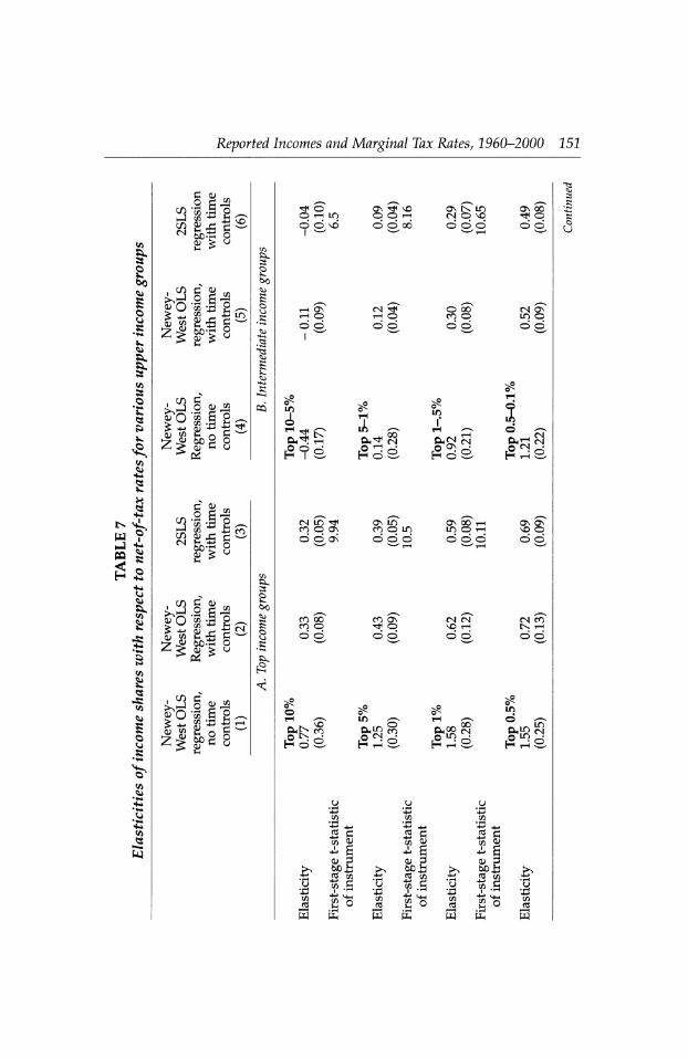
Reported Incomes and Marginal Tax Rates, 1960-2000 151
t? 0) 9 S-3
SR?S' ?J0-1
' 3 .?? ? * ?P LO
"Mr
O? '*
k5>
.6 SR
.So
5 S
o g C? t? c? rt
O) ̂ Jh o ?Tj g
Is o
^ o OH IT)
?;
Os "^ ^D O O rH ? ? 00
OS IN LO
? ? ?
On 00 ^tf O
? ? U
rH O ? CD
I W
CN ̂ rH O
? ?
O 00 CO o CD ?
CN ON LO O
?
H^? rH
CN LC Tt< CO O OS
C^ CN
tS?S
On LO room
LO r
rH ^
^? CN F?S
ON 00 rH LO O rH
T, _ <n
C^CN^ fSrnS
ON ON N?> O
CO 00 CO O
? ? CO ON
^ O ? ?
CN CN V?> rH
CN CO L\ rH
in ^ OhLO S
FrnB
Lfi
rSrnB
u
C? 43
' ? ?
? .5
s C? ' O -M S ci ? s
CTj
C?
w
u 43 C?
w
.S
w Ph
u '43
W
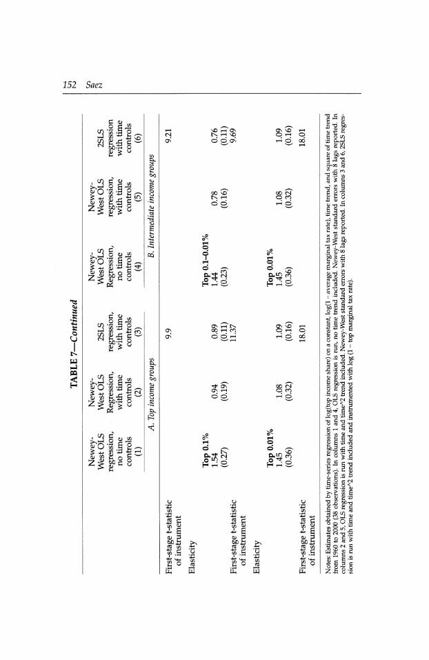
252 Soez
Po O c?
go 53 c?
2|
c? XI S ^
all" ?18
o o> ̂ 3 *c? ? P c? . t?
o
s ? u
^O 'S -S ̂ ^
OjO 55 c?
c? S g. c? x! 43 .
2|8>S?'
?
CN ON n?) rH On
Nh\D On 'vO rH O rH O HO 00
00 v?> LN rH
00 CN O CO
^^ CO
F^o
ON ON
ON rH LN 00 rH CO
? ? rH
On ^0 r-i O rH O
tF On ON rH ? ?
? ^
FrnB
00 CN O CO H ?
O ?* Ce?
F^o
43
t? S ? ?
c? .S
tk^ g
o 43 c?
H
U '43 c?
'5 +*
to a> ? B
S g 43 c?
w
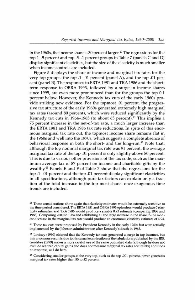
Reported Incomes and Marginal Tax Rates, 1960-2000 153
in the 1960s, the income share is 30 percent larger.40 The regressions for the
top 1-.5 percent and top .5-1 percent groups in Table 7 (panels C and D)
display significant elasticities, but the size of the elasticity is much smaller
when income controls are included.
Figure 5 displays the share of income and marginal tax rates for the
very top groups: the top .1-.01 percent (panel A), and the top .01 per cent (panel B). The responses to ERTA 1981 and TRA 1986 and the short
term response to OBRA 1993, followed by a surge in income shares
since 1995, are even more pronounced than for the groups the top 0.1
percent below. However, the Kennedy tax cuts of the early 1960s pro vide striking new evidence. For the topmost .01 percent, the progres sive tax structure of the early 1960s generated extremely high marginal tax rates (around 80 percent), which were reduced significantly by the
Kennedy tax cuts in 1964-1965 (to about 65 percent).41 This implies a
75 percent increase in the net-of-tax rate, a much larger increase than
the ERTA 1981 and TRA 1986 tax rate reductions. In spite of this enor
mous marginal tax rate cut, the topmost income share remains flat in
the 1960s and well into the 1970s, which suggests a complete absence of
behavioral response in both the short- and the long-run.42 Note that,
although the top nominal marginal tax rate was 91 percent, the average
marginal tax rate of the top .01 percent is only slightly above 80 percent. This is due to various other provisions of the tax code, such as the max
imum average tax of 87 percent on income and charitable gifts by the
wealthy.43 Panels E and F of Table 7 show that the regressions for the
top .1-01 percent and the top .01 percent display significant elasticities in all specifications, although pure tax factors can explain only a frac
tion of the total increase in the top most shares once exogenous time
trends are included.
40 These considerations show again that elasticity estimates would be extremely sensitive to
the time period considered. The ERTA 1981 and OBRA 1993 episodess would produce 0 elas
ticity estimates, and TRA 1986 would produce a sizable 0.93 estimate (comparing 1986 and
1988). Comparing 2000 to 1984 and attributing all the large increase in the share to the mod
est decrease in the marginal tax rate would produce an enormous elasticity estimate of 4.94.
41 These tax cuts were proposed by President Kennedy in the early 1960s but were actually
implemented by the Johnson administration after Kennedy's death in 1963.
42 Lindsey (1990) claimed that the Kennedy tax cuts generated a surge in top incomes, but
this erroneous result is due to his casual examination of the tabulations published by the 1RS.
Goolsbee (1999) makes a more careful use of the same published data (although he does not
exclude realized capital gains and does not measure marginal tax rates accurately) and finds no response, as I do here.
43 Considering smaller groups at the very top, such as the top .001 percent, never generates
marginal tax rates higher than 80 to 82 percent.
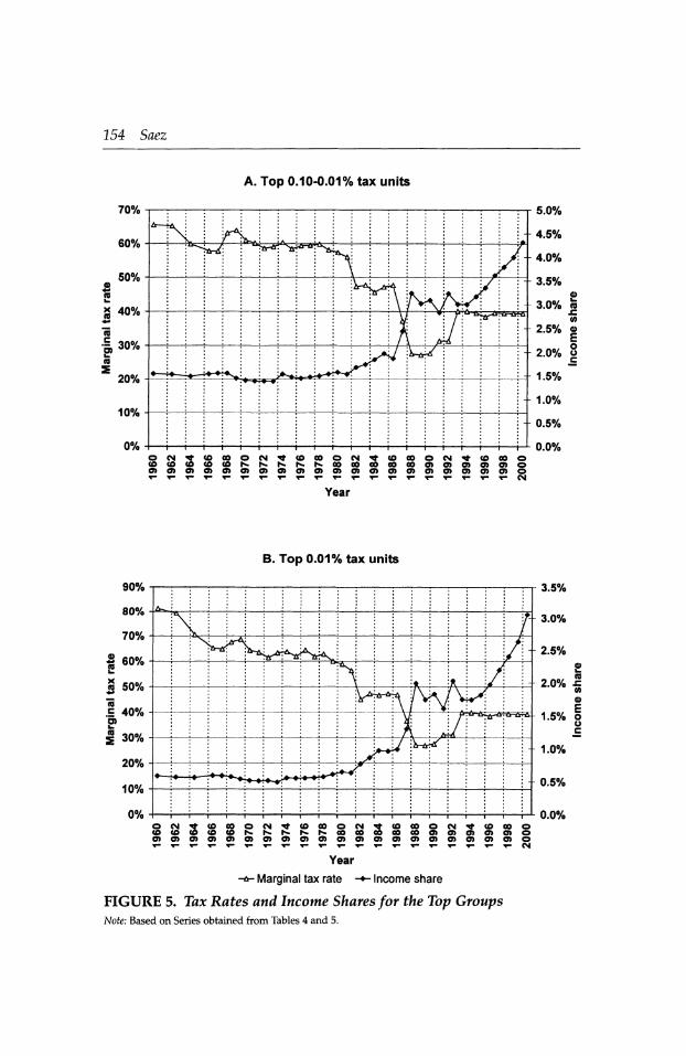
154 Saez
A. Top 0.10-0.01% tax units
? (O CM^<OOOOCM^t<OOOOCMTttOCOOCM^t(OCOO (0<0(0(0SSSSS00000000000)0)O)0)0)O
0)0)0)0>O)O)O)O)0>O)O)OO)0)O>O)OO>0)O T-T-T-T-^T-T-T--r-T-<?-^-T-T--r-T-T-T-T-<M
Year
B. Top 0.01% tax units
90%
-i-1-1?i?i?i?i?i?i?i?i-1?i
OM^tOCOOCM^COOOOCM^COOOOCM^COOOO <0<0<o<0<0N.i^i**h?h?eooocoeoooo>o>0>o>o>o O)0>O>O)O>0)O>O>OO)0>O>0>O>0>OO)0>O)G>O T-*-T-*-T-*-*-T-T-^Y-*-T-*-T-Y-T-*-*-T-<M
Year
-&- Marginal tax rate - -
Income share
FIGURE 5. Tax Rates and Income Shares for the Top Groups Note: Based on Series obtained from Tables 4 and 5.
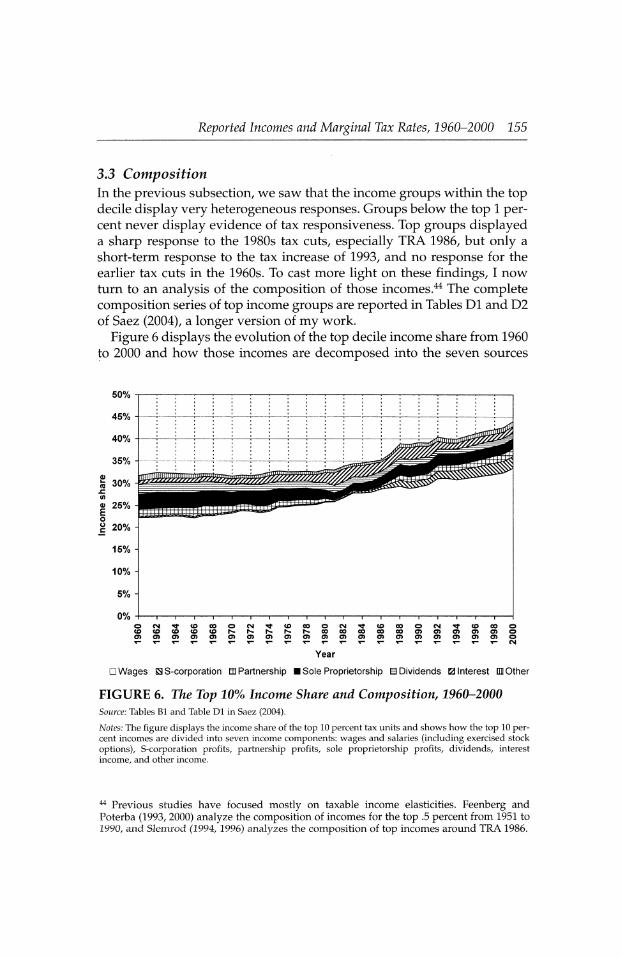
Reported Incomes and Marginal Tax Rates, 1960-2000 155
3.3 Composition In the previous subsection, we saw that the income groups within the top decile display very heterogeneous responses. Groups below the top 1 per cent never display evidence of tax responsiveness. Top groups displayed a sharp response to the 1980s tax cuts, especially TRA 1986, but only a
short-term response to the tax increase of 1993, and no response for the
earlier tax cuts in the 1960s. To cast more light on these findings, I now
turn to an analysis of the composition of those incomes.44 The complete
composition series of top income groups are reported in Tables Dl and D2
of Saez (2004), a longer version of my work.
Figure 6 displays the evolution of the top decile income share from 1960
to 2000 and how those incomes are decomposed into the seven sources
50%
?CN^,COCO?CN'<tCOCOOCN*1' cococococoh-h-r^h-h-cococo cd O CD CD CD CD CD CD CD CD O CD CD
CO CO O CM CO CO O CD CD CD CD CD
Tf CO CO CD CD CD
Wages H S-corporation Efl Partnership
Year
I Sole Proprietorship ?Dividends 0Interest CHOther
FIGURE 6. The Top 10% Income Share and Composition, 1960-2000
Source: Tables Bl and Table Dl in Saez (2004).
Notes: The figure displays the income share of the top 10 percent tax units and shows how the top 10 per cent incomes are divided into seven income components: wages and salaries (including exercised stock
options), S-corporation profits, partnership profits, sole proprietorship profits, dividends, interest
income, and other income.
44 Previous studies have focused mostly on taxable income elasticities. Feenberg and
Poterba (1993, 2000) analyze the composition of incomes for the top .5 percent from 1951 to
1990, and Slemrod (1994, 1996) analyzes the composition of top incomes around TRA 1986.
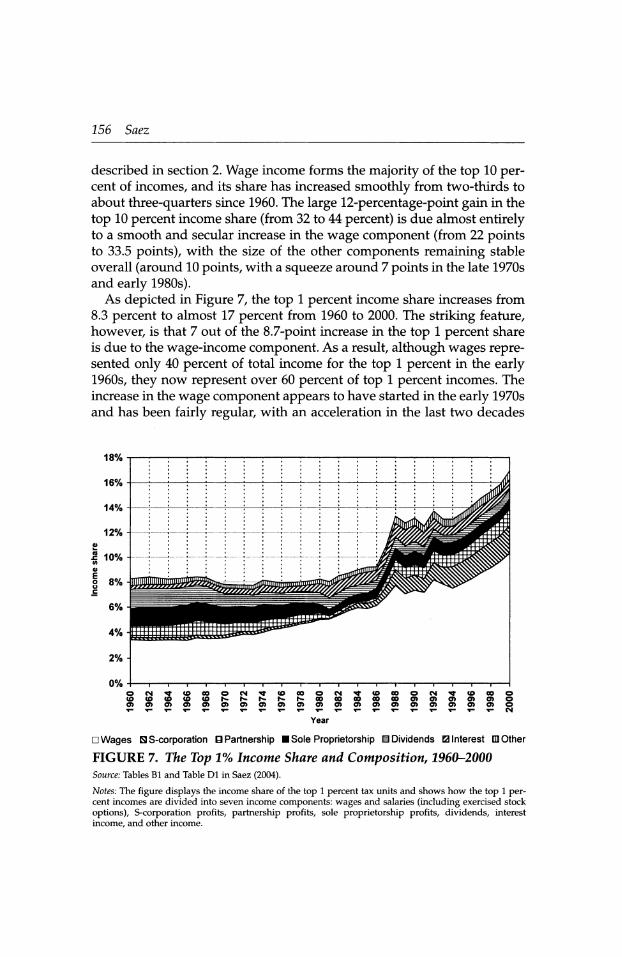
156 Saez
described in section 2. Wage income forms the majority of the top 10 per cent of incomes, and its share has increased smoothly from two-thirds to
about three-quarters since 1960. The large 12-percentage-point gain in the
top 10 percent income share (from 32 to 44 percent) is due almost entirely to a smooth and secular increase in the wage component (from 22 points to 33.5 points), with the size of the other components remaining stable
overall (around 10 points, with a squeeze around 7 points in the late 1970s
and early 1980s). As depicted in Figure 7, the top 1 percent income share increases from
8.3 percent to almost 17 percent from 1960 to 2000. The striking feature,
however, is that 7 out of the 8.7-point increase in the top 1 percent share
is due to the wage-income component. As a result, although wages repre sented only 40 percent of total income for the top 1 percent in the early 1960s, they now represent over 60 percent of top 1 percent incomes. The
increase in the wage component appears to have started in the early 1970s
and has been fairly regular, with an acceleration in the last two decades
Year
D Wages H S-corporation Q Partnership Sole Proprietorship S Dividends 0 Interest DB Other
FIGURE 7. The Top 1% Income Share and Composition, 1960-2000 Source: Tables Bl and Table Dl in Saez (2004).
Notes: The figure displays the income share of the top 1 percent tax units and shows how the top 1 per cent incomes are divided into seven income components: wages and salaries (including exercised stock
options), S-corporation profits, partnership profits, sole proprietorship profits, dividends, interest
income, and other income.
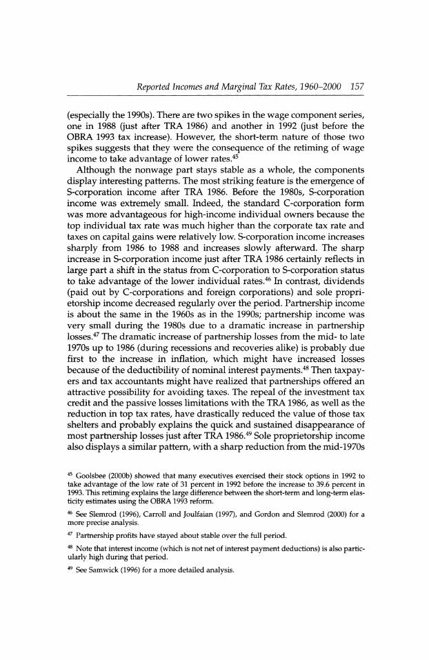
Reported Incomes and Marginal Tax Rates, 1960-2000 157
(especially the 1990s). There are two spikes in the wage component series, one in 1988 (just after TRA 1986) and another in 1992 (just before the
OBRA 1993 tax increase). However, the short-term nature of those two
spikes suggests that they were the consequence of the retiming of wage income to take advantage of lower rates.45
Although the nonwage part stays stable as a whole, the components
display interesting patterns. The most striking feature is the emergence of
S-corporation income after TRA 1986. Before the 1980s, S-corporation income was extremely small. Indeed, the standard C-corporation form
was more advantageous for high-income individual owners because the
top individual tax rate was much higher than the corporate tax rate and
taxes on capital gains were relatively low. S-corporation income increases
sharply from 1986 to 1988 and increases slowly afterward. The sharp increase in S-corporation income just after TRA 1986 certainly reflects in
large part a shift in the status from C-corporation to S-corporation status
to take advantage of the lower individual rates.46 In contrast, dividends
(paid out by C-corporations and foreign corporations) and sole propri
etorship income decreased regularly over the period. Partnership income
is about the same in the 1960s as in the 1990s; partnership income was
very small during the 1980s due to a dramatic increase in partnership losses.47 The dramatic increase of partnership losses from the mid- to late
1970s up to 1986 (during recessions and recoveries alike) is probably due
first to the increase in inflation, which might have increased losses
because of the deductibility of nominal interest payments.48 Then taxpay ers and tax accountants might have realized that partnerships offered an
attractive possibility for avoiding taxes. The repeal of the investment tax
credit and the passive losses limitations with the TRA 1986, as well as the
reduction in top tax rates, have drastically reduced the value of those tax
shelters and probably explains the quick and sustained disappearance of
most partnership losses just after TRA 1986.49 Sole proprietorship income
also displays a similar pattern, with a sharp reduction from the mid-1970s
45 Goolsbee (2000b) showed that many executives exercised their stock options in 1992 to
take advantage of the low rate of 31 percent in 1992 before the increase to 39.6 percent in
1993. This retiming explains the large difference between the short-term and long-term elas
ticity estimates using the OBRA 1993 reform.
46 See Slemrod (1996), Carroll and Joulfaian (1997), and Gordon and Slemrod (2000) for a
more precise analysis. 47
Partnership profits have stayed about stable over the full period. 48 Note that interest income (which is not net of interest payment deductions) is also partic
ularly high during that period.
See Samwick (1996) for a more detailed analysis.
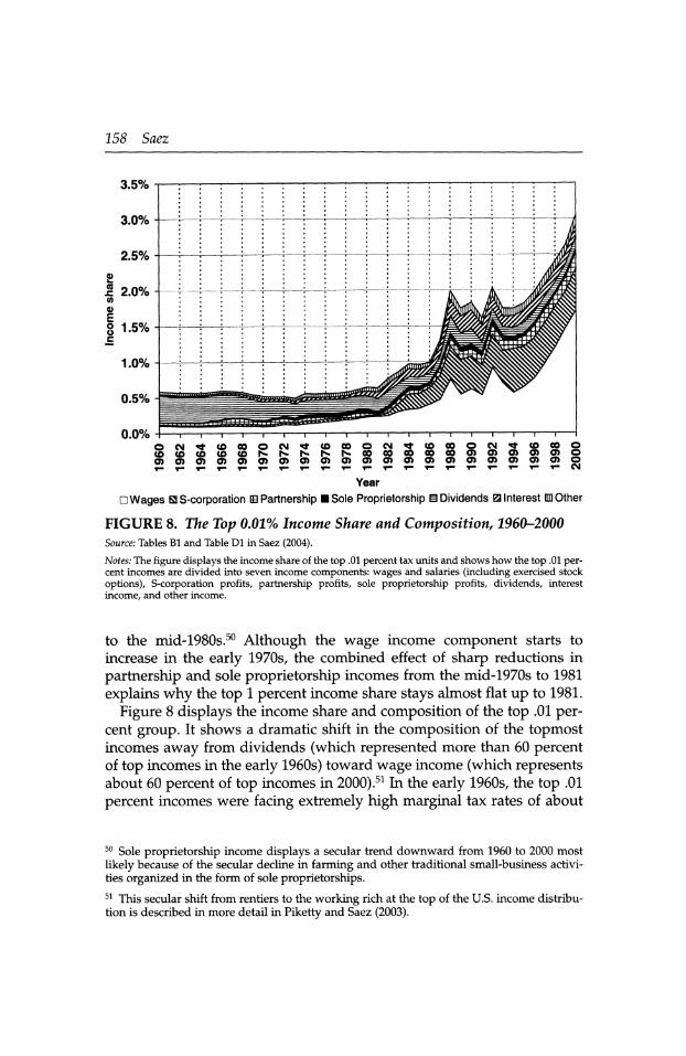
158 Saez
0.0% H-1-1-1-1-i-1-1-1-1-i-1-1-1-1-1-1-1-1-r OCM^COeOOCM^COOOOCM^COOOOCMTrCOCOO
<O<0<0<0<Oh?l^h?h?h?COCOCOOOCOO>O>O>0>O>O O)O)O)O)O)O)O)O)O)O)O)O)(J)O)0)(J)O)O)0)O)O
T-Y-Y-T-T-Y-T-T-Y-Y-Y-Y-T-T-Y-Y-Y-Y-Y-T-CM
Year
D Wages H S-corporation B Partnership ISole Proprietorship S Dividends Sinterest ED Other
FIGURE 8. The Top 0.01% Income Share and Composition, 1960-2000
Source: Tables Bl and Table Dl in Saez (2004).
Notes: The figure displays the income share of the top .01 percent tax units and shows how the top .01 per cent incomes are divided into seven income components: wages and salaries (including exercised stock
options), S-corporation profits, partnership profits, sole proprietorship profits, dividends, interest
income, and other income.
to the mid-1980s.50 Although the wage income component starts to
increase in the early 1970s, the combined effect of sharp reductions in
partnership and sole proprietorship incomes from the mid-1970s to 1981
explains why the top 1 percent income share stays almost flat up to 1981.
Figure 8 displays the income share and composition of the top .01 per cent group. It shows a dramatic shift in the composition of the topmost incomes away from dividends (which represented more than 60 percent of top incomes in the early 1960s) toward wage income (which represents about 60 percent of top incomes in 2000).51 In the early 1960s, the top .01
percent incomes were facing extremely high marginal tax rates of about
50 Sole proprietorship income displays a secular trend downward from 1960 to 2000 most
likely because of the secular decline in farming and other traditional small-business activi
ties organized in the form of sole proprietorships. 51 This secular shift from rentiers to the working rich at the top of the U.S. income distribu
tion is described in more detail in Piketty and Saez (2003).
Reported Incomes and Marginal Tax Rates, 1960-2000 159
80 percent on average (while tax rates on long-term capital gains were
around 25 percent). Thus, dividends were a disadvantageous form of
income for the rich, which suggests that these top-income earners had lit
tle control over the form of payment and thus might have been passive investors. The Kennedy tax cuts did not reduce the top individual rate
enough (the top rate became 70 percent) to make the S-corporation form
attractive relative to the C-corporation form, which explains perhaps the
contrast in behavioral responses between the Kennedy tax cuts and the
tax changes of the 1980s. This situation shows, as argued by Slemrod and
Kopczuk (2002), that the elasticity of reported incomes is not a constant
parameter but may be extremely sensitive to the legal structure and the
complete tax environment for corporations and individuals. The share of
dividends falls regularly over the period, while the share of wage income
starts to increase in 1971. By 1979, the wage component overtakes the div
idend component. Figure 8 shows clearly that ERTA 1981 produced a sud
den burst of S-corporation income (which was negligible up to 1981)
mostly likely because of a shift from C-corporations to S-corporations.52 Note that the increase in S-corporation income is concentrated mostly in
the top .01 percent and does not happen at all for groups below the top .1
percent. This situation is consistent with the tax minimization explana tion: ERTA 1981 decreased marginal tax rates significantly only for groups above the top .1 percent, for whom the Subchapter S status started to
become attractive when the top individual rate was reduced to 50 per cent.53 Figure 8 shows that almost all the increase in top incomes from
1981 to 1984, first documented by Lindsey (1987), is also due to the surge in S-corporation income. The wage component increases as well but with
no noticeable break in the upward trend around ERTA 1981.54 The S
corporation component increases again sharply from 1986 to 1988 and
then stays about stable afterward. The wage component also presents a
spike in 1988 and in 1993, but these spikes seem to be short-term
responses in a generally upward trending curve. The tax cuts of the 1960s,
although extremely large, did not generate any behavioral response per
haps because top individual rates remained substantially higher than the
corporate and capital gains tax rate and thus did not induce top-income
taxpayers to switch corporate income toward individual income.
52 As discussed in section 2.1, this phenomenon has been well documented in the case of
TRA 1986. 53 From 1980 to 1986, the corporate tax rate was 42 percent. 54 Because of the maximum tax of 50 percent on labor income enacted in 1971-1972, the
marginal tax rates for top wage incomes actually did not change much with ERTA; see
section 3.4.
160 Saez
Therefore, to sum up, the dramatic increase in top income shares is due
primarily to a secular increase in the wage income component starting in
the early 1970s, and the large tax changes of TRA 1986 and OBRA 1993
seem to have generated only short-term spikes in the overall upward and
accelerating trend of the wage component.55 The tax cuts of the 1980s have
generated a surge in business income taxed at the individual level. ERTA
1981 created a surge in S-corporation income for the topmost groups of
the income distribution. With TRA 1986, S-corporation income surged for
all upper-income groups. Partnership income also rose dramatically
immediately after TRA 1986 mostly because of the disappearance of part
nership losses. These business income components have remained rela
tively stable after TRA 1986, which suggests they were the consequence of a one-time shift from the corporate sector and the one-time closing of the
partnership loss tax shelters. The top tax rate increase of 1993 to 39.6 per cent (with a corporate tax rate of 35 percent) was not large enough to
induce businessowners to switch back to the C-corporation status. As a
result, OBRA 1993 did not produce any long-term income shifting away from the individual sector, and its only effect seems to have been a short
term retiming of salary income. The surge in business income reported on
individual returns in the 1980s cannot be interpreted as a supply-side suc
cess because most of these individual income gains came either at the
expense of taxable corporate income or could have been obtained from the closing of tax shelters after the imposition of stricter rules on losses
from passive businesses.56 Therefore, the success or failure of the tax cuts
at generating additional economic activity must be deferred to a more
precise analysis of the central wage income component, to which we now
turn.
3.4 Top Wage Incomes
We have seen that most of the increase in top income shares since the
1970s is actually due to a sharp increase in the wage income component. The time pattern of marginal tax rates for wage income is not the same as
the pattern for other forms of income because of the introduction of the
maximum tax rate on earned income in 1971, which reduced the top rate
55 Top income shares are flat before 1981, masking the increase in the wage component,
because of a large decline in partnership and sole proprietorship income, due in turn per
haps to high interest rates and the development of tax shelters in the 1970s. Partnership income and, to a lesser extent, sole proprietorship income increased back to their early 1970s
levels immediately after TRA 1986.
56 It is doubtful that the decrease in tax rates, by reducing the incentives to avoid taxes, was
necessary to eliminate abusive partnership losses (as argued, for example, in Samwick, 1996) because partnership losses were almost nonexistent before the late 1970s, a time when tax
rates were extremely high.
Reported Incomes and Marginal Tax Rates, 1960-2000 161
for earned income from 70 percent (the top rate on other income) to 60
percent in 1971 and then 50 percent starting in 1972.57 This provision became irrelevant in 1982, when the top tax rate for any income source
was reduced from 70 percent to 50 percent. Therefore, analyzing the
wage income component separately is of particular interest. All the top wage income share series and corresponding average marginal tax rates for
wage income are reported in Tables 8 and 9, respectively. As for average income, the evolution of average real wage income
series (for the full population) does not appear to be correlated with the
evolution of marginal tax rates. Figure 9 shows the pattern of real incomes
and marginal tax rates for the bottom 99 percent wage earners (panel A) and the top 1 percent wage earners (panel B). The bottom 99 percent have
experienced no real growth in wage income since 1972, and the pattern of
changes in real wages does not seem to be related to changes in marginal tax rates. In contrast, top 1 percent wage income earners experienced
accelerating growth over the 1960 to 2000 period, with almost a tripling in real wage income since the early 1970s. Consistent with the pattern of
the wage component for overall income, top wage income earners ex
perienced spikes just after TRA 1986 and just before OBRA 1993, clear
evidence of short-term responses (or retiming) of labor income compen sation. However, the long-run pattern seems to be an extraordinary and
accelerating growth independent of the tax developments because mar
ginal tax rates on these wage income earners were about the same, around
40 percent, in the mid-1960s and in the most recent years. Indeed, the sec
ular growth in top wages starts in the early 1970s, a time when marginal tax rates were actually increasing (due mostly to the progressive nature of the income tax structure and the resulting bracket creep). To understand
better this unprecedented increase in top wage incomes, it is useful to
consider smaller groups within the top 1 percent, as I did for overall income.
Table 10 produces the same regressions as Table 7 but for wage incomes
instead of overall income.58 The shares of the bottom groups of the top decile below the top 1 percent (top 10-5 percent and top 5-1 percent) dis
play low elasticities, while all groups within the top 1 percent display sig nificant elasticities when no time trend is included. The elasticities
increase sharply from 0.3 to 2.5 as we move up the wage income distribution
57 As described in Slemrod (1994), the marginal income tax rate on labor income could be
higher than these limits in several cases because of the interaction of this provision with the
regular schedule.
58 I have omitted the IV estimates in the case of wages because the first stage is not as strong as in the case of income and because the estimates are more noisy.
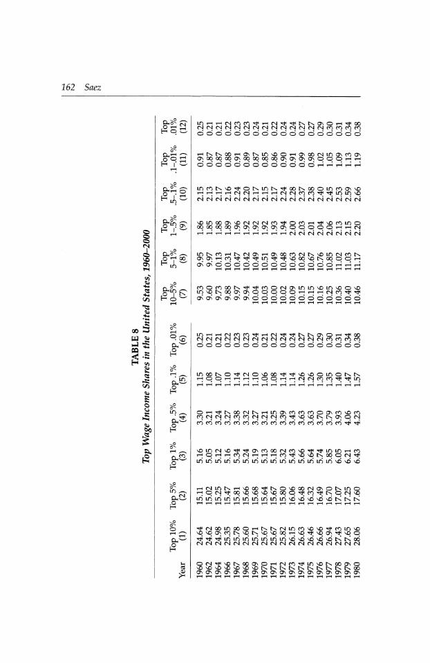
262 Saez
ON.
2
H o O
F I
e3?^
(MfN|fNM(N(MMNMCNCSfM(NNcOCOCOCO ??????????????????
HNN00H0\Mf)v0OHO\00Mlfj0\r0a ONoqoqoqo\oqoqoqoqa\aN(>ONqoqHH ?????????????^-HrHT-HrHT-H
NrN?N(N?HHHNHNHdcN?(N?NcNfSN
^lT)OOON^CN(SCNCO^O^H^M)fOLnO oqoqoqoqoNONO\CT\C\0\qqqqqHHN
ir)NcOHNNO\HO\?cONNv?lONcnN
O^as?????????????T-HrHrH
rooroooN^^cooMOMriin^invoovo in^0N000\0\OOOOOHHHNn^^
^o\o?o\o\o\dddddc)6c)ddd6
GO S
S-s
o
IP a.
Oh"
eS
?
r
eu
e2
<0
2
iDHHMrtfO^Hfsj^^NNONOH^OO
??????????????????
in??NO^(NO\D00^^^\?OinONN HqqHHHHqqHHN(Nicoro^^in
OH^NX(NNHlOONCOCDCOOO\CO^>CO cocNr^cNcoco(N(Nr|fO^^)\?lst\ONqfN
LOLOLOLntriiiSiiSLnioLOLniriinLoiiS^v?vo
H(NinNH^ooo^NovDoofSO\OMno ^prsj^oqvqvqvovqoqo^cn^iNpiNvo
LOlnliSlOliSLfilr)lnlril?S^ov?v?v>?v?^s;I^.*^^s!
^(Nooif)OOOHNNcsinco^)^^mir]vo \?^)ONCON^Nv?\?OOHV?^vOO\^v?O
tNtNCNtN?NtNtN(N(N(NtN(N|tNtNtNtN(N?N
ON^v?N00^OH(Ncn^ir)vON00O\O
OnO\ \G\OnQ\G\OnOnOnQ\OvOnOnOn On On On
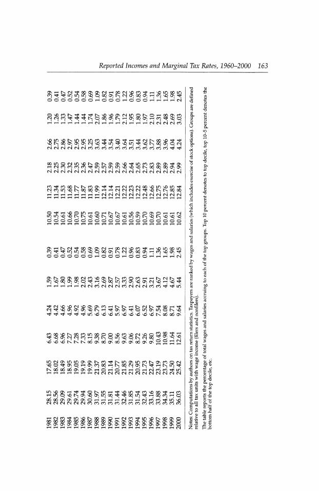
Reported Incomes and Marginal Tax Rates, 1960-2000 163
ON^tNtN^OOONONtNrHOOCNVOCO^rH^DLDOOLO cn^^ir)iniiNvoqoqoNis(NONoqa\Hcoqa\^
???????rH???rH???rHi-HrHr-iH
r^CN^rtrfH^^pOOONlN^ONOqONrHCO^vqp HHHHHHHdrirHHNHHHlNfsiHrjc'i
NO^cxjONONONtN^q^io^^ioT^vqiNjoqoNpcN
xinotNiiNv?NONN^ON^^incocooNON^aN T^rsjcncncocor^ifNLQinLnvqvqvqbvoocsqoqoNON (NJHcN(N?NHdddHNH(McsdH(NH(N?(N?
CO^COOOINlNCOON^^rHrslCOtNOONOLONOLO^ tNCOLONDtNOOCXJONrHrHrslrjC^CNj^vqiNl^C?Oq
HHHHHHHHN(N?N(NCN?(N?(NtN?CNHfN(N?
O^H\?OlOHOHNNH^(J\Oa\OHHM
????????????????????
NHOO(N|vDcn^H\?if)QOir) OqON?s.CNjONOqONrHCON?ON'^
????OO?^CJ??rH???T-HrHT-Hi-HCN
ON ^H IN <N ̂ 00 ON i co ^ ^ m Loin ^? '
O\NO0N00CSc0v0 0NNNc0Oc0HHNfgN^ Ln^^ONONp^rH^oqii^cooNvqoNrNivqrHvqTt
^T^'rHrHrHrsiHcoHcsicsicOCsiCsic^COr?^T^?S
tN^NqONONONNq^rHTfONON^OLnONLOOlN^O ^rt?^^^T^iiSv?s?VsDLn^v?vov?\oKodo6o?
C000^N00Win00OO^C0v0(N^o2S^S ^v?O\^<NriHfONOif)^ON(NOOTl:a)^^
li^r^ONinirsOsoNtNco^iNLnoNirNcoiNONcoocsi ^q^osqHONfOoqHiNoq(Na\N^HNif)^
ISo6oOo6(^ON(J\HdHdHHdH(Nc?c?^I/i
T^ii^pvqtNONvqoNii^oq^rfoqLnr^rHoqcorHp coo?oNONoNONO^T^^rHrvi^THrsicoc?'^Ln^o rvitNr^r^cNtNcncncocncococococotrNc^cncrico
ooooooooooooooooooonononononononononono OnOnOnOnOnONOnOnOnOnOnOnOnOnOnOnOnOnOnO T-HrH^HrHr?lT-HrHrHrHT?It-Ht-Ht?Ir-HrHT-HrHT-Ht?ItN
2 O
t? O
I
O)
.S ?s
t?
bO
a,
Oh p
O
o
eu ?2
CL,
g
1
bC t?
?2
il S'5 O (y
fe t?
* ?
^ 42
S 19 as S n O o
y; ai q3
5"! ?J
cu ?i be a?
cu t3
8 g n .3 2? +
2? ?Si
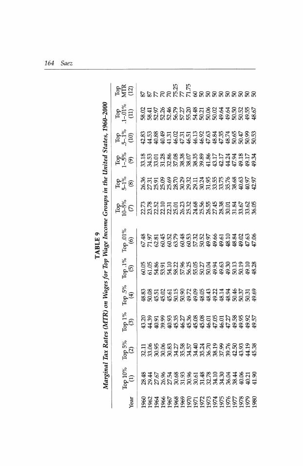
264 Saez
O*}
?5
CO
2
^3
^ lo
H^S
,8^1 ^?;
LO LO (N LN
lNLNLNOOI?Sl>^0000000000 OOOOLNLNLNLNlNLNMDLOLOLOLOLOLOLOLOLO
(N|HN\?vOONNOOOH\?CS^^OCSinN p^ONCN^t^tNtN^cNjppvqvqLqLqLOvq o6odHr4cNvoL<Lo^???oNON??oNcx5 LOLOLOLOLOLOLOLOLOLOLOLO'^f'^LOLO'^'^
cofoxoNHfNiHHfncNcn^in^LONONco ooLooo^coocOLOr-HONvoootrNLNvq^oNLq ri^d?Hvoisvuv?v?No?iso?dddd
HLqq^joqqcoqcooqoqHHtNjONHHco CO^COrHeNLNOOoOoOONrHCOCN^LNONONON COCOCOCOCOCOCOCOCOCO^^T?Hr?HTtHT?HrtHT}H
vDHHOM^OONCNH^iniOLDvO?OCONN cncooNqvqisNcorHfNONLnisN^qvqaNOs v?i\i?inioo?doNO\dHr?foino6dd(N eNCNcNc^tNCNicocNitNcocoerjcococo^^T^
cooo(NOHHcoNoo\?if)inooH^N(sm NKinrHcoqNcovqinio^coqoqvq^oq rsicnHrsitNLovdiiSTfiiSNoKo?o^coco^D e^rsic^CNieNCNieNCsjtNesitNCNc^cococococo
si
Jf>l
?5
?
a.?
e2
Oh
e2
asi
t9
r
CO
2
00 tx ^ ON 00 Ttf I NHCN?ddcndotsdo?o?a\o?o?o\NK
LOrJO\OOfOCN(NN^)HO^tN|fO^) 'LOLNTfLOCOLOONVONOT-HOOONOO
LOLONOrHOtN^LOLOL^^^COOCOONOOO qooooNH{sa\(NiofNO(??^fOHHHN dH^co^oONv?indda\a\ONodoNo6
vovoLoinLOiOLOiniDioin^^Ttinio^^
rOODHCNHinONOMOfOM^^vONHON oqoir>qvprHa\Nqq^(NHO\^coco^D o??lololo??ononooo?ono?oo???on TtlLO^^^LOLO'^'<*Ttt'^TtHr^TjHLOLOLO'^
oc^HONcnLON^ooxHinHNxintNiN rvJCOONONONt^fNCOppppptNLOONONLQ C?^OO?OLO^dLdLOLONULNvdKo?ONONON T^ ^^ ̂ ^ CO ^^ ^i ^^ ^^ ^f ^^ ''?t^ ^^ ^^ "^? ̂̂ ^^ ^?^ ̂ ^
HVOlDvDCONOONO^OONON^OrtONOO HqoNqoqr^inin^(NisHONis?Na\Hco Hc?dddTjHifi^T}?iov?ootsa\(Ncn^io
en co co co co co co co co cococncoco^^rt^t
OO^N^^OOCOV?HOOOOOO^^VOHO ^^vooNinqosos^D^tsHfoq^qNON QOoNN^tsOHOOHN^^voodddH CNicNic^r^tNcocococococococococo^^^
OtN-H^NoOONOHMCO^LO^NOOONO
OnOnOnOnOnOnOnOnOnOnONOnOnOnOnONOnOn
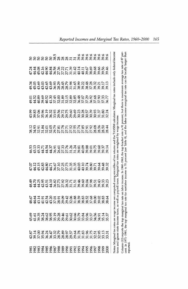
Reported Incomes and Marginal Tax Rates, 1960-2000 165
lo vqvsONqvqv^vqvsO^ OOOOOOO?oOOOOOt-h^hOnOnOnOnOnOnOnO?
LOLOLOLOIi^LOCOCNtNCNCOCOCOCOCOCOCOCOCOCO
^rfoOvOO^OONOtN^HONCM^T-HlNONOONOVsD^O rsj^pTHONoqLOcotNLNjCo^T^rHvqvqvqv^Lq^
N^inH^rfvoNNNHHodaNcxJaNON^aN Tt^^^^^COfN?NCNCOCOr?H^COCOCOCOCOCO
^LOONCOLOONCOONLOONOOLOONtNOOOOCNrHLNCO copNqpvqvqoNCN|rfLNONvqoNCNj^cNco(NrH ONLococoHcovdododod^rHodoNooKo?o?ONON r^rf^^TtrticOCNtNCNCOCOCOCOCOCOCOCOCOcO
t-icmononcmolooonloonlooolnoncnooocoln pLOOOvOLOCO^pOOrHOOOq^pCNON^qONCOlN
'do\dHN(SHfSfN?CN^NNvOlNts'N ^O T^co^^cocococococococococococococo
ON rf I
ONCO^NOONCNCON?CMLOOONCOOOINONCOLXO'^ ONOOpONrHCOO^^LNLN^Nqr^CNLOCOONCOOqCN C?ONLNLOV?NOc?ONONONONO?OOOOOrH^HCN?
^COCOCOCOCOCOCNtNtNfNCNCOCOCOCOCOCOCOCO
MCOH^H?NONHOOHfNLO^lOHtNOO^O^ t-hononoooolnoolnlnlolotnooononololo^ oo^Ht^Hcn?onlnlnlnKlninlnKlno?o?o?o? COCOCOCOCOCOCNCNltNCNCN|CNCNltN(NCNCNCNCN|CN
?.S
H .5 ̂
fOfOrOHrtNrHHCn^)^)^HONOOHinONi< inHcoNincooNvqrtNiNNoqqoqqtsv?rtH
r^^r?H^^^cOtNCNlCNCOCOCO'^COCOCOCOCOCO
lN(NLOCOOrHlNOLOCOLOLOCOOTtlOrHr}HOOCN
IN 33 LO tN ̂ ^ ^Jl TJJ1 T?p T^l ̂ ^i *^1 vOLNLnLNt?i t?lOOONOOONONONON COtNCNCNCOCO^^COCOCOCOCOCO
On ?
ONOLOLOrHOCMCOCMtNT?IrHVOO^OOrHCOCOCO ^N(NONiOHoqiso\rtisift^voqo\in^W(Nj o?^^Hc?^^iNLNo?^^oigNgiLNoigNONgi ^^ ^J^ ̂ ^ ^^ "?T^ "?p COCMCMCNICOCOCOCOCOCOCOCOCOCO
NqNqrHONLqcsjpONprtjpoqLooqLqvqcqpoqNq 06rfCOrHCN?COlN00ONONHrH0d0?0dlNO?o?0600 rf^Tf^r^rfCOCNlCNlCNlCOCOCOCOCOCOCOCOCOCO
ONrHLO^CNLOON00NOrHCNNOONTfvOtNNOT-H"^tN vqvqcocNjNqoNr^tN^NqvqvDLNoqoNLqLOONrHco i?St-hono?o?o?loonono?ooc?c?coco^^l?lo
^^cocococococmtncnlcocococococococococo
OOrHpONCNjr^COlNOqONLqNDLNOqONLNLOONrHCO Ha\Nlf?v?V?f?0?06u?ONONHHHHfN?tNCf5cO ^COCOCOCOCOCOCNCNCMCNCMCOCOCOCOCOCOCOCO
rHtNCO^LOvOLNOOONOrHCMCO^LONOLNOOONO ooooooooooooooooooonononononononononono ONOnOnOnOnOnOnOnOnOnOnonOnOnOnOnOnOnOnO t?It?It?It?It?It?It?It?It?It?It?IrHT?It?It?It?It?It-Ht-HCN
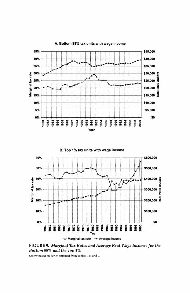
A. Bottom 99% tax units with wage income
OCN^-COCOOCN^-CDOOOCNTj-COOOOCN-^tCOOOO (0(O(O(0(ONSSSS(O(O(OOO(O9)O)O)O)O>O
Year
B. Top 1% tax units with wage income
60%
? CM "^ CO CO ? CM CO CO CO CO CO h- h O) O) O) o o> O) O)
-<* CO CO ? CM N S S 00 00 ._ O) O) O O) O) O) S
(O co 00 00
O CM ^t CO CO O) O) O) O) o o> O) O) o> o>
$600,000
$500,000
$400,000 ?2 (0 o o
$300,000 ?
$200,000 S.
$100,000
$0
Year
-*- Marginal tax rate -*- Average income
FIGURE 9. Marginal Tax Rates and Average Real Wage Incomes for the
Bottom 99% and the Top 1%
Source: Based on Series obtained from Tables 1, 8, and 9.
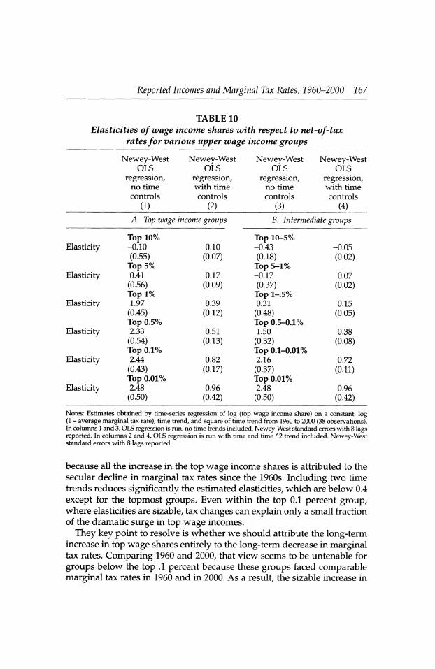
Reported Incomes and Marginal Tax Rates, 1960-2000 167
TABLE 10 Elasticities of wage income shares with respect to net-of-tax
rates for various upper wage income groups
Newey-West OLS
regression, no time
controls
(i)
Newey-West OLS
regression, with time
controls
(2)
Newey-West OLS
regression, no time
controls
(3)
Newey-West OLS
regression, with time
controls
(4)
Elasticity
Elasticity
Elasticity
Elasticity
Elasticity
Elasticity
A. Top wage income groups B. Intermediate groups
Top 10% -0.10
(0.55) Top 5%
0.41
(0.56) Top 1%
1.97
(0.45) Top 0.5%
2.33
(0.54) Top 0.1%
2.44
(0.43) Top 0.01%
2.48
(0.50)
0.10
(0.07)
0.17
(0.09)
0.39
(0.12)
0.51
(0.13)
0.82
(0.17)
0.96
(0.42)
Top 10-5% -0.43
(0.18) Top 5-1% -0.17
(0.37) Top l-.5%
0.31
(0.48) Top 0.5-0.1%
1.50
(0.32) Top 0.1-0.01%
2.16
(0.37) Top 0.01%
2.48
(0.50)
-0.05
(0.02)
0.07
(0.02)
0.15
(0.05)
0.38
(0.08)
0.72
(0.11)
0.96
(0.42)
Notes: Estimates obtained by time-series regression of log (top wage income share) on a constant, log (1
- average marginal tax rate), time trend, and square of time trend from 1960 to 2000 (38 observations).
In columns 1 and 3, OLS regression is run, no time trends included. Newey-West standard errors with 8 lags reported. In columns 2 and 4, OLS regression is run with time and time A2 trend included. Newey-West standard errors with 8 lags reported.
because all the increase in the top wage income shares is attributed to the secular decline in marginal tax rates since the 1960s. Including two time trends reduces significantly the estimated elasticities, which are below 0.4
except for the topmost groups. Even within the top 0.1 percent group, where elasticities are sizable, tax changes can explain only a small fraction of the dramatic surge in top wage incomes.
They key point to resolve is whether we should attribute the long-term increase in top wage shares entirely to the long-term decrease in marginal tax rates. Comparing 1960 and 2000, that view seems to be untenable for
groups below the top .1 percent because these groups faced comparable marginal tax rates in 1960 and in 2000. As a result, the sizable increase in
168 Saez
the top 1-.5 percent and top .5-1 percent wage income shares cannot be
due entirely to marginal tax rates.
The problem is more complicated for the topmost groups (within the
top .1 percent) because these groups experienced much larger gains but
also experienced a nontrivial decline in marginal tax rates. Undoubtedly, a reason for the huge increase in top wage income shares (the top .01 per cent share increased more than tenfold, from .21 percent in 1970 to 2.45
percent in 2000) has been the development of stock options. Stock options also create lumpiness in wage compensation because they are exercised
by executives only once every few years. As a result, the top .01 percent
might be extremely large in recent years because, in any given year, top most wage earners are executives who happen to exercise their stock
options in that particular year. The stock-option phenomenon, however, has clearly increased the average compensation of top executives because
the top 1 percent (which certainly includes almost all the top employees
receiving large option grants, even when they do not exercise stock
options) more than doubles from 5.1 to 12.6 percent from 1970 to 2000.
Thus, the extraordinary increase in top wage incomes, a phenomenon
certainly closely related to the explosion in the compensation of chief
executive officers (CEOs) and other top executives and sports, movie, and
television stars, appears too large to have been solely the direct conse
quence of the tax reductions through supply-side effects. Furthermore, the surge in top wages is not related closely enough to the timing of the
tax cuts to suggest a direct and simple causal link. Particularly surprising is the surge in top wages since 1994, in spite of the significant tax increase
in 1993, which makes the secular reduction in marginal tax rates faced by top wage groups appear rather small.59
A more pertinent issue is whether this surge in top wages could have
occurred had the tax structure remained the same as in the early 1960s, when the working rich had to pay in taxes more than three-quarters of
their compensation. It is plausible to think that the drastic reduction in
top marginal tax rates, which started in the 1960s, opened the possibility of the dramatic increase in top wages that started in the 1970s and accel
erated in the 1980s and 1990s. Of course, it is impossible to provide a con
vincing answer to that important issue by looking only at individual
income tax statistics in the United States. A promising approach would be
to analyze executive compensation data. Many have researched executive
59 Companies might have started granting stock options more aggressively after TRA1986,
however, because of the decrease in individual tax rates. These options can be exercised (and thus appear on individual income tax returns) only several years later. However, Hall and
Murphy (2003) show that grants of stock options, valued using the Black-Scholes formula, increased significantly after the tax increase of 1993.
Reported Incomes and Marginal Tax Rates, 1960-2000 169
compensation; see Murphy (1999) for a survey. Although many studies
explain the disparity of CEO pay in cross-sectional data, no convincing explanation for the time-series evidence seems to have been provided.60 If the dramatic surge in top compensation is not fully explained by a com
parable surge in the marginal productivity of top executives, then this lack is evidence of a market failure, which would certainly change the
welfare and tax policy analysis that I presented above. Perhaps top exec
utive pay may now be aligned with marginal product and was below market value before. Note, however, that the surge in the top 1 percent
salaries since the early 1970s has been accompanied by dismal growth for the bottom 99 percent salary earners and thus does not seem to have
had a positive impact on the vast majority of working families. An alter native way to make progress in our understanding is by looking at com
parable experiences in other countries, a point to which I now turn for the conclusion.
4. CONCLUSION: INTERNATIONAL COMPARISONS
No other country offers such a large body of empirical analysis on behav ioral responses to individual income taxation as does the United States.
Recently, however, several studies have produced series of top income shares using tax return data. Although these studies do not produce cor
responding series of marginal tax rates, as I have shown here, interesting findings emerge.
First, enormous heterogeneity exists in the behavior of top income shares in recent decades across countries. Some countries, such as the
United Kingdom (Atkinson, 2002) or Canada (Saez and Veall, 2003) have
experienced notable increases in top income shares, although these increases have not been as pronounced as in the United States. In contrast, countries from continental Europe, such as France (Piketty, 2003), the
Netherlands (Atkinson and Salverda, 2003), and Switzerland (Dell,
Piketty, and Saez, 2003), have experienced either decline or little change in
top income shares since 1960.
Second, the U.K. experience seems to be the closest to the U.S. experi ence. Top income shares in the United Kingdom started increasing exactly in 1979, when the top rate declined from 98 to 75 percent, although the concomitant increase seems modest relative to the size of the net-of-tax
60 It is quite telling to read in the recent survey of Hall and Murphy (2003), two prominent and conservative researchers in this field, that their best explanation for the surge in stock
option compensation was that "boards and managers falsely perceive stock options to be
inexpensive because of accounting and cash-flow considerations."
170 Saez
increase at the top.61 In 1988, the top rate was further decreased to 40 per cent and has not changed since then. In contrast to the United States, how
ever, the increase in top share has been relatively smooth since 1979, with no break around the tax changes. Studying the composition and estimat
ing precisely the marginal tax rates faced by top U.K. income-taxpayers seems to be a priority in understanding whether the recent increase in top incomes is due to the tax developments.62
Third, Canada has experienced a surge in top incomes significantly
larger than the increase in the United Kingdom (although smaller than
that in the United States) and, as in the United States, this increase has
been due to a dramatic increase in top salaries since the early 1980s. In
contrast to the United States, however, top incomes in Canada have not
experienced, large tax cuts since the 1960s.63 Thus, the dramatic increase
in top incomes in Canada cannot be attributed solely to fiscal develop ments in Canada. Saez and Veall (2003) argue that the threat of emigration
to the United States has forced Canadian companies to increase the pay of
their top employees if they want to retain them, thereby replicating in
Canada the dramatic U.S. increase in top employees' pay. If the migration
explanation is correct, it implies that the surge in top wage incomes in the
United States is a real phenomenon and not a unique consequence of the
repackaging of income to avoid taxes.
Last, France, the Netherlands, and Switzerland have experienced rela
tively small changes in their top tax rates, in contrast to the United States
and the United Kingdom. Piketty (1999) shows that the small changes in
the French top tax rates generated small shortterm responses from top income taxpayers but that those responses do not seem to persist over
time. Switzerland has lower top-income tax rates than does the United
States (around 35 percent when adding federal, cantonal, and local
income taxes), but has much lower top income shares than does the
United States (the top 1 percent share was around 8-9 percent in the
1990s, while it was between 13 and 17 percent in the United States). In sum, high income tax rates do not seem to account for the differences
in top income shares across countries, although it is more debatable
whether they can account for a substantial part of the time-series pattern within countries. Therefore, a systematic analysis of top incomes in countries
61 It might be the case, however, that for the top .1 percent incomes, the average decline in
marginal tax rates has been much more modest.
62 Dilnot and Kell (1988) try to analyze this issue but have access only to a single year of
micro tax returns and have to rely on aggregate numbers for their time-series analysis. 63 The top income tax rate in Canada, including provincial taxes, was about 50 percent in
2000.
Reported Incomes and Marginal Tax Rates, 1960-2000 171
that have experienced drastic cuts in top income tax rates in recent
decades, as in the United States and the United Kingdom, would be of
most interest. Those results could teach us whether a dramatic cut in top rates is necessarily associated with a rise in top incomes.
REFERENCES
Atkinson, Anthony (2002). "Top Incomes in the United Kingdom over the Twentieth Century." Nuffield College, Oxford. Mimeo.
Atkinson, Anthony, and Wiemer Salverda (2003). "Top Incomes in the Netherlands and the United Kingdom over the Twentieth Century." Nuffield
College, Oxford. Mimeo.
Auerbach, Alan (1988). "Capital Gains Taxation in the United States." Brookings Papers on Economic Activity 2:595-631.
Auten, Gerald, and Robert Carroll (1999) "The Effect of Income Taxes on Household Behavior." Review of Economics and Statistics 81(4):681-693.
Bertrand, Marianne, Esther Duflo, and Sendhil Mullaina than (2002). "How Much Should We Trust Differences-in-Differences Estimates?" NBER Working Paper no. 8841. March. Forth-coming in Quarterly Journal of Economics. 119(1), 2004.
Carroll, Robert (1998). "Tax Rates, Taxpayer Behavior, and the 1993 Tax Act." Office of Tax Analysis, U.S. Department of the Treasury. Working paper. November Number 79.
Carroll, Robert, and David Joulfaian (1997). "Taxes and Corporate Choice of
Organizational Form." Office of Tax Analysis, U.S. Department of the Treasury.
Working Paper no. 73. October.
Dell, Fabien, Thomas Piketty, and Emmanuel Saez (2003). "The Evolution of Income and Wealth Concentration in Switzerland over the 20th Century."
University of California. Mimeo.
Dilnot, Andrew, and Michael Kell (1988). "Top-Rate Tax Cuts and Incentives: Some Empirical Evidence." Fiscal Studies 9:70-92.
Eissa, Nada (1995). "Taxation and Labor Supply of Married Women: The Tax Reform Act of 1986 as a Natural Experiment." NBER Working Paper no. 5023.
February. Eissa, Nada, and Jeffrey Liebman (1996). "Labor Supply Response to the Earned
Income Tax Credit." Quarterly Journal of Economics 111:605-637.
Feenberg, Daniel, and Elisabeth Coutts (1993). "An Introduction to the TAXSIM Model." Journal of Policy Analysis and Management 12(1):189-194.
Feenberg, Daniel, and James Poterba (1993). "Income Inequality and the Incomes of Very High Income Taxpayers: Evidence from Tax Returns." Tax Policy and the
Economy 7:145-177.
Feenberg, Daniel, and James Poterba (2000). "The Income and Tax Share of Very High Income Households, 1960-1995". American Economic Review 90(2):264-270.
Feldstein, Martin (1995). "The Effect of Marginal Tax Rates on Taxable Income: A Panel Study of the 1986 Tax Reform Act." Journal of Political Economy 103(3):551-572.
Feldstein, Martin (1999). "Tax Avoidance and the Deadweight Loss of the Income Tax". Review of Economics and Statistics 81(4):674-680.
172 Saez
Feldstein, Martin, and Daniel Feenberg (1996). "The Effect of Increased Tax Rates on Taxable Income and Economic Efficiency: A Preliminary Analysis of the 1993 Tax Rate Increases". Tax Policy and the Economy 10:89-117.
Goolsbee, Austan (1999). "Evidence on the High-Income Laffer Curve from Six Decades of Tax Reform." Brookings Papers on Economic Activity 2:1-47.
Goolsbee, Austan (2000a). "It's Not About the Money: Why Natural Experiments Don't Work on the Rich." In Does Atlas Shrug? The Economic Consequences of Taxing the Rich, J. Slemrod (ed.). Cambridge, MA: Harvard University Press.
Goolsbee, Austan (2000b). "What Happens When You Tax the Rich? Evidence from Executive Compensation." Journal of Political Economy 108(2):352-378.
Gordon, Roger, and Joel Slemrod (2000). "Are 'Real' Responses to Taxes Simply Income Shifting Between Corporate and Personal Tax Bases?" In Does Atlas
Shrug? The Economic Consequences of Taxing the Rich, J. Slemrod (ed.). Cambridge, MA: Harvard University Press.
Gruber, Jonathan, and Emmanuel Saez (2002). "The Elasticity of Taxable Income: Evidence and Implications." Journal of Public Economics 84:1-32.
Hall, Brian, and Kevin Murphy (2003). "The Trouble with Stock Options". NBER
Working Paper no. 9784. June.
Katz, Lawrence, and David Autor (1999). "Changes in the Wage Structure and
Earnings Inequality." In Handbook of Labor Economics, Volume 3 A, O. Ashenf elter and D. Card (eds.). Amsterdam: North-Holland.
Kopczuk, Wojciech (2003). "Tax Bases, Tax Rates and the Elasticity of Reported Income." NBER Working Paper no. 10044. October.
Liebman, Jeffrey, and Richard Zeckhauser (2003). "Schmeduling". Harvard
University. Mimeo.
Lindsey, Lawrence (1987). "Individual Taxpayer Response to Tax Cuts: 1982-1984, with Implications for the Revenue Maximizing Tax Rate." Journal of Public Economics 33:173-206.
Lindsey, Lawrence (1990). The Growth Experiment: How the New Tax Policy Is
Transforming the U.S. Economy. New York: Basic Books, Inc.
Meyer, Bruce, and Daniel Rosenbaum (2001). "Welfare, the Earned Income Tax
Credit, and the Labor Supply of Single Mothers." Quarterly Journal of Economics
116(3):1063-1114. Mirrlees, James A. (1971). "An Exploration in the Theory of Optimal Income
Taxation." Review of Economic Studies 38:175-208.
Murphy, Kevin J. (1999). "Executive Compensation." In Handbook of Labor
Economics, Volume 3B, O. Ashenf elter and D. Card (eds.). Amsterdam: North Holland.
Piketty, Thomas (1999). "Les Hauts Revenus Face aux Modifications des Taux
Marginaux Sup?rieurs de l'Imp?t sur le Revenu en France, 1970-1996." Economie et Pr?vision 138-139:25-60.
Piketty, Thomas (2003). "Income Inequality in France, 1901-1998." Journal of Political Economy 111(5):1004-1042.
Piketty, Thomas, and Emmanuel Saez (2003). "Income Inequality in the United States, 1913-1998." Quarterly Journal of Economics 118(l):l-39. Series updated to
year 2000 at http://www.nber.org/papers/w8467 (accessed March, 2003). Saez, Emmanuel (2001). "Using Elasticities to Derive Optimal Income Tax Rates."
Review of Economic Studies 68:205-229.
Saez, Emmanuel (2002). "Do Taxpayers Bunch at Kink Points?" University of California. Mimeo.
Reported Incomes and Marginal Tax Rates, 1960-2000 173
Saez, Emmanuel (2003). "The Effect of Marginal Tax Rates on Income: A Panel
Study of 'Bracket Creep'." Journal of Public Economics 87:1231-1258. Saez, Emmanuel (2004). "Reported Incomes and Marginal Tax Rates, 1960-2000:
Evidence and Policy Implications." NBER Working Paper no. 10273 February. Saez, Emmanuel, and Michael Veall (2003). "The Evolution of High Incomes in
Canada, 1920-2000." NBER Working Paper no. 9607. April. Sammartino, Frank, and David Weiner (1997). "Recent Evidence on
Taxpayers'
Response to the Rate Increases in the 1990s." National Tax Journal 50(3):683-705. Samwick, Andrew (1996). "Tax Shelters and Passive Losses After the Tax Reform
Act of 1986." In Empirical Foundations of Household Taxation, M. Feldstein and J. Poterba (eds.). Chicago, IL: University of Chicago Press.
Scholes, Myron, and Mark A. Wolf son (1992). Taxes and Business Strategy: A Planning Approach. New York: Prentice Hall.
Slemrod, Joel (1994). "On the High Income Laffer Curve." In Tax Progressivity and Income Inequality, J. Slemrod (ed.). Cambridge, England: Cambridge University
Press, 177-210.
Slemrod, Joel (1995). "Income Creation or Income Shifting? Behavioral Responses to the Tax Reform Act of 1986." American Economic Review 85(2): 175-180.
Slemrod, Joel (1996). "High Income Families and the Tax Changes of the 1980s: The Anatomy of Behavioral Response." In Empirical Foundations of Household Taxation, M. Feldstein and J. Poterba (eds.). Chicago, IL: University of Chicago Press.
Slemrod, Joel (1998). "Methodological Issues in Measuring and Interpreting Taxable Income Elasticities." National Tax Journal 51 (4):773-788.
Slemrod, Joel, and Jonathan Bakija (2001). "Growing Inequality and Decreased Tax Progressivity." In Inequality and Tax Policy, K. Hassett (ed.). Washington DC American Enterprise Institute Press.
Slemrod, Joel, and Wojciech Kopczuk (2002). "The Optimal Elasticity of Taxable Income." Journal of Public Economics 84(1):91-112.
Stewart, Kenneth J., and Stephen B. Reed (1999). "CPI Research Series Using Current Methods, 1978-98." Monthly Labor Review 122(6):29-38.