Report Reconstructing Visual Experiences from Brain Activity ...
17
Current Biology 21, 1641–1646, October 11, 2011 ª2011 Elsevier Ltd All rights reserved DOI 10.1016/j.cub.2011.08.031 Report Reconstructing Visual Experiences from Brain Activity Evoked by Natural Movies Shinji Nishimoto, 1 An T. Vu, 2 Thomas Naselaris, 1 Yuval Benjamini, 3 Bin Yu, 3 and Jack L. Gallant 1,2,4, * 1 Helen Wills Neuroscience Institute 2 Joint Graduate Group in Bioengineering 3 Department of Statistics 4 Department of Psychology University of California, Berkeley, Berkeley, CA 94720, USA Summary Quantitative modeling of human brain activity can provide crucial insights about cortical representations [1, 2] and can form the basis for brain decoding devices [3–5]. Recent functional magnetic resonance imaging (fMRI) studies have modeled brain activity elicited by static visual patterns and have reconstructed these patterns from brain activity [6–8]. However, blood oxygen level-dependent (BOLD) signals measured via fMRI are very slow [9], so it has been difficult to model brain activity elicited by dynamic stimuli such as natural movies. Here we present a new motion-energy [10, 11] encoding model that largely overcomes this limitation. The model describes fast visual information and slow hemo- dynamics by separate components. We recorded BOLD signals in occipitotemporal visual cortex of human subjects who watched natural movies and fit the model separately to individual voxels. Visualization of the fit models reveals how early visual areas represent the information in movies. To demonstrate the power of our approach, we also con- structed a Bayesian decoder [8] by combining estimated encoding models with a sampled natural movie prior. The decoder provides remarkable reconstructions of the viewed movies. These results demonstrate that dynamic brain activity measured under naturalistic conditions can be de- coded using current fMRI technology. Results Many of our visual experiences are dynamic: perception, visual imagery, dreaming, and hallucinations all change continuously over time, and these changes are often the most compelling and important aspects of these experiences. Obtaining a quantitative understanding of brain activity underlying these dynamic processes would advance our understanding of visual function. Quantitative models of dynamic mental events could also have important applications as tools for psychiatric diagnosis and as the foundation of brain machine interface devices [3–5]. Modeling dynamic brain activity is a difficult technical prob- lem. The best tool available currently for noninvasive mea- surement of brain activity is functional magnetic resonance imaging (fMRI), which has relatively high spatial resolution [12, 13]. However, blood oxygen level-dependent (BOLD) signals measured using fMRI are relatively slow [9], especially when compared to the speed of natural vision and many other mental processes. It has therefore been assumed that fMRI data would not be useful for modeling brain activity evoked during natural vision or by other dynamic mental processes. Here we present a new motion-energy [10, 11] encoding model that largely overcomes this limitation. The model separately describes the neural mechanisms mediating visual motion information and their coupling to much slower hemo- dynamic mechanisms. In this report, we first validate this en- coding model by showing that it describes how spatial and temporal information are represented in voxels throughout visual cortex. We then use a Bayesian approach [8] to combine estimated encoding models with a sampled natural movie prior, in order to produce reconstructions of natural movies from BOLD signals. We recorded BOLD signals from three human subjects while they viewed a series of color natural movies (20 3 20 at 15 Hz). A fixation task was used to control eye position. Two separate data sets were obtained from each subject. The training data set consisted of BOLD signals evoked by 7,200 s of color natural movies, where each movie was presented just once. These data were used to fit a separate encoding model for each voxel located in posterior and ventral occipitotemporal visual cortex. The test data set consisted of BOLD signals evoked by 540 s of color natural movies, where each movie was repeated ten times. These data were used to assess the accuracy of the encoding model and as the targets for movie reconstruction. Because the movies used to train and test models were different, this approach provides a fair and objec- tive evaluation of the accuracy of the encoding and decoding models [2, 14]. BOLD signals recorded from each voxel were fit separately using a two-stage process. Natural movie stimuli were first filtered by a bank of neurally inspired nonlinear units sensitive to local motion-energy [10, 11]. L1-regularized linear regres- sion [15, 16] was then used to fit a separate hemodynamic coupling term to each nonlinear filter (Figure 1; see also Sup- plemental Experimental Procedures available online). The regularized regression approach used here was optimized to obtain good estimates even for computational models con- taining thousands of regressors. In this respect, our approach differs from the regression procedures used in many other fMRI studies [17, 18]. To determine how much motion information is available in BOLD signals, we compared prediction accuracy for three different encoding models (Figures 2A–2C): a conventional static model that includes no motion information [8, 19], a nondirectional motion model that represents local motion energy but not direction, and a directional model that repre- sents both local motion energy and direction. Each of these models was fit separately to every voxel recorded in each subject, and the test data were used to assess prediction accuracy for each model. Prediction accuracy was defined as the correlation between predicted and observed BOLD signals. The averaged accuracy across subjects and voxels in early visual areas (V1, V2, V3, V3A, and V3B) was 0.24, 0.39, and 0.40 for the static, nondirectional, and directional encoding models, respectively (Figures 2D and 2E; see Figure S1A for subject- and area-wise comparisons). This *Correspondence: [email protected]
Transcript of Report Reconstructing Visual Experiences from Brain Activity ...
Current Biology 21, 1641–1646, October 11, 2011 ª2011 Elsevier Ltd All rights reserved DOI 10.1016/j.cub.2011.08.031
ReportReconstructing Visual Experiences fromBrain Activity Evoked by Natural Movies
Shinji Nishimoto,1 An T. Vu,2 Thomas Naselaris,1
Yuval Benjamini,3 Bin Yu,3 and Jack L. Gallant1,2,4,*1Helen Wills Neuroscience Institute2Joint Graduate Group in Bioengineering3Department of Statistics4Department of PsychologyUniversity of California, Berkeley, Berkeley, CA 94720, USA
Summary
Quantitative modeling of human brain activity can providecrucial insights about cortical representations [1, 2] and
can form the basis for brain decoding devices [3–5]. Recentfunctional magnetic resonance imaging (fMRI) studies have
modeled brain activity elicited by static visual patterns andhave reconstructed these patterns from brain activity [6–8].
However, blood oxygen level-dependent (BOLD) signalsmeasured via fMRI are very slow [9], so it has been difficult
to model brain activity elicited by dynamic stimuli such asnatural movies. Here we present a new motion-energy [10,
11] encoding model that largely overcomes this limitation.Themodel describes fast visual information and slow hemo-
dynamics by separate components. We recorded BOLDsignals in occipitotemporal visual cortex of human subjects
who watched natural movies and fit the model separatelyto individual voxels. Visualization of the fit models reveals
how early visual areas represent the information in movies.
To demonstrate the power of our approach, we also con-structed a Bayesian decoder [8] by combining estimated
encoding models with a sampled natural movie prior. Thedecoder provides remarkable reconstructions of the viewed
movies. These results demonstrate that dynamic brainactivity measured under naturalistic conditions can be de-
coded using current fMRI technology.
Results
Many of our visual experiences are dynamic: perception, visualimagery, dreaming, and hallucinations all change continuouslyover time, and these changes are often the most compellingand important aspects of these experiences. Obtaining aquantitative understanding of brain activity underlying thesedynamic processes would advance our understanding ofvisual function. Quantitative models of dynamic mental eventscould also have important applications as tools for psychiatricdiagnosis and as the foundation of brain machine interfacedevices [3–5].
Modeling dynamic brain activity is a difficult technical prob-lem. The best tool available currently for noninvasive mea-surement of brain activity is functional magnetic resonanceimaging (fMRI), which has relatively high spatial resolution[12, 13]. However, blood oxygen level-dependent (BOLD)signals measured using fMRI are relatively slow [9], especiallywhen compared to the speed of natural vision and many other
mental processes. It has therefore been assumed that fMRIdata would not be useful for modeling brain activity evokedduring natural vision or by other dynamic mental processes.Here we present a new motion-energy [10, 11] encoding
model that largely overcomes this limitation. The modelseparately describes the neural mechanisms mediating visualmotion information and their coupling to much slower hemo-dynamic mechanisms. In this report, we first validate this en-coding model by showing that it describes how spatial andtemporal information are represented in voxels throughoutvisual cortex.We then use a Bayesian approach [8] to combineestimated encoding models with a sampled natural movieprior, in order to produce reconstructions of natural moviesfrom BOLD signals.We recorded BOLD signals from three human subjects while
they viewedaseries of color naturalmovies (20� 320� at 15Hz).A fixation task was used to control eye position. Two separatedata sets were obtained from each subject. The training dataset consisted of BOLD signals evoked by 7,200 s of colornatural movies, where each movie was presented just once.These data were used to fit a separate encoding model foreach voxel located in posterior and ventral occipitotemporalvisual cortex. The test data set consisted of BOLD signalsevoked by 540 s of color natural movies, where each moviewas repeated ten times. These data were used to assess theaccuracy of the encoding model and as the targets for moviereconstruction. Because the movies used to train and testmodels were different, this approach provides a fair and objec-tive evaluation of the accuracy of the encoding and decodingmodels [2, 14].BOLD signals recorded from each voxel were fit separately
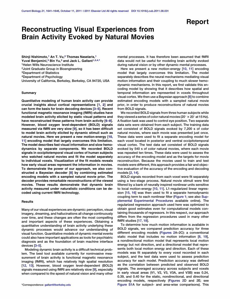
using a two-stage process. Natural movie stimuli were firstfiltered by a bank of neurally inspired nonlinear units sensitiveto local motion-energy [10, 11]. L1-regularized linear regres-sion [15, 16] was then used to fit a separate hemodynamiccoupling term to each nonlinear filter (Figure 1; see also Sup-plemental Experimental Procedures available online). Theregularized regression approach used here was optimized toobtain good estimates even for computational models con-taining thousands of regressors. In this respect, our approachdiffers from the regression procedures used in many otherfMRI studies [17, 18].To determine how much motion information is available in
BOLD signals, we compared prediction accuracy for threedifferent encoding models (Figures 2A–2C): a conventionalstatic model that includes no motion information [8, 19],a nondirectional motion model that represents local motionenergy but not direction, and a directional model that repre-sents both local motion energy and direction. Each of thesemodels was fit separately to every voxel recorded in eachsubject, and the test data were used to assess predictionaccuracy for each model. Prediction accuracy was definedas the correlation between predicted and observed BOLDsignals. The averaged accuracy across subjects and voxelsin early visual areas (V1, V2, V3, V3A, and V3B) was 0.24,0.39, and 0.40 for the static, nondirectional, and directionalencoding models, respectively (Figures 2D and 2E; seeFigure S1A for subject- and area-wise comparisons). This*Correspondence: [email protected]
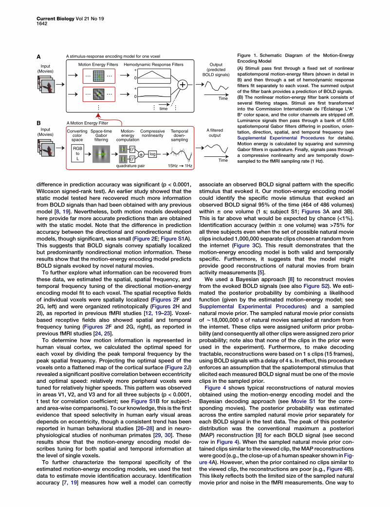
difference in prediction accuracy was significant (p < 0.0001,Wilcoxon signed-rank test). An earlier study showed that thestatic model tested here recovered much more informationfrom BOLD signals than had been obtained with any previousmodel [8, 19]. Nevertheless, both motion models developedhere provide far more accurate predictions than are obtainedwith the static model. Note that the difference in predictionaccuracy between the directional and nondirectional motionmodels, though significant, was small (Figure 2E; Figure S1A).This suggests that BOLD signals convey spatially localizedbut predominantly nondirectional motion information. Theseresults show that the motion-energy encoding model predictsBOLD signals evoked by novel natural movies.
To further explore what information can be recovered fromthese data, we estimated the spatial, spatial frequency, andtemporal frequency tuning of the directional motion-energyencoding model fit to each voxel. The spatial receptive fieldsof individual voxels were spatially localized (Figures 2F and2G, left) and were organized retinotopically (Figures 2H and2I), as reported in previous fMRI studies [12, 19–23]. Voxel-based receptive fields also showed spatial and temporalfrequency tuning (Figures 2F and 2G, right), as reported inprevious fMRI studies [24, 25].
To determine how motion information is represented inhuman visual cortex, we calculated the optimal speed foreach voxel by dividing the peak temporal frequency by thepeak spatial frequency. Projecting the optimal speed of thevoxels onto a flattened map of the cortical surface (Figure 2J)revealed a significant positive correlation between eccentricityand optimal speed: relatively more peripheral voxels weretuned for relatively higher speeds. This pattern was observedin areas V1, V2, and V3 and for all three subjects (p < 0.0001,t test for correlation coefficient; see Figure S1B for subject-and area-wise comparisons). To our knowledge, this is the firstevidence that speed selectivity in human early visual areasdepends on eccentricity, though a consistent trend has beenreported in human behavioral studies [26–28] and in neuro-physiological studies of nonhuman primates [29, 30]. Theseresults show that the motion-energy encoding model de-scribes tuning for both spatial and temporal information atthe level of single voxels.
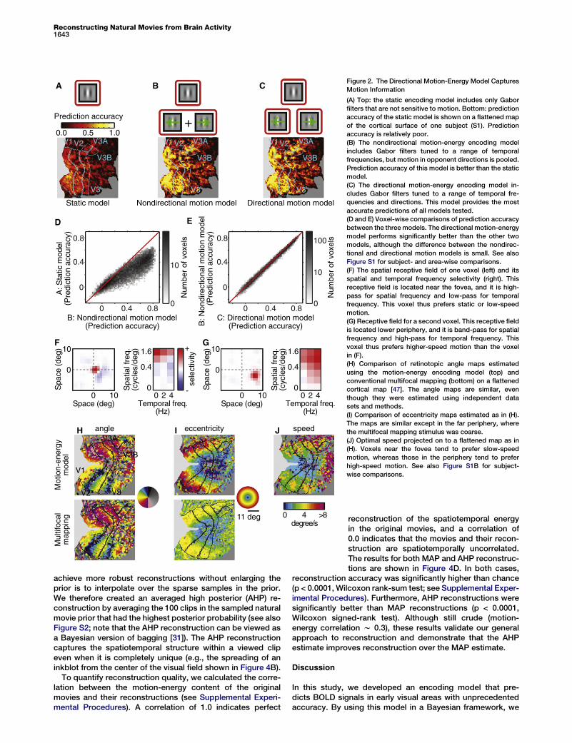
To further characterize the temporal specificity of theestimated motion-energy encoding models, we used the testdata to estimate movie identification accuracy. Identificationaccuracy [7, 19] measures how well a model can correctly
associate an observed BOLD signal pattern with the specificstimulus that evoked it. Our motion-energy encoding modelcould identify the specific movie stimulus that evoked anobserved BOLD signal 95% of the time (464 of 486 volumes)within 6 one volume (1 s; subject S1; Figures 3A and 3B).This is far above what would be expected by chance (<1%).Identification accuracy (within 6 one volume) was >75% forall three subjects even when the set of possible natural movieclips included 1,000,000 separate clips chosen at random fromthe internet (Figure 3C). This result demonstrates that themotion-energy encoding model is both valid and temporallyspecific. Furthermore, it suggests that the model mightprovide good reconstructions of natural movies from brainactivity measurements [5].We used a Bayesian approach [8] to reconstruct movies
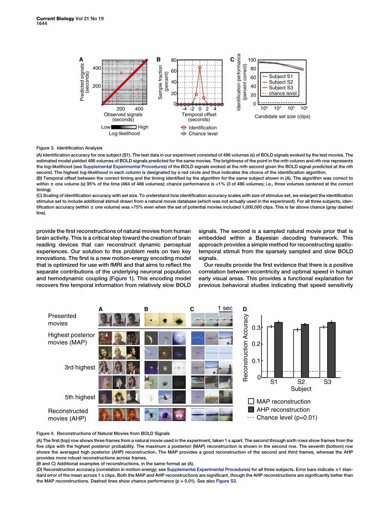
from the evoked BOLD signals (see also Figure S2). We esti-mated the posterior probability by combining a likelihoodfunction (given by the estimated motion-energy model; seeSupplemental Experimental Procedures) and a samplednatural movie prior. The sampled natural movie prior consistsof w18,000,000 s of natural movies sampled at random fromthe internet. These clips were assigned uniform prior proba-bility (and consequently all other clips were assigned zero priorprobability; note also that none of the clips in the prior wereused in the experiment). Furthermore, to make decodingtractable, reconstructions were based on 1 s clips (15 frames),using BOLD signals with a delay of 4 s. In effect, this procedureenforces an assumption that the spatiotemporal stimulus thatelicited each measured BOLD signal must be one of the movieclips in the sampled prior.Figure 4 shows typical reconstructions of natural movies
obtained using the motion-energy encoding model and theBayesian decoding approach (see Movie S1 for the corre-sponding movies). The posterior probability was estimatedacross the entire sampled natural movie prior separately foreach BOLD signal in the test data. The peak of this posteriordistribution was the conventional maximum a posteriori(MAP) reconstruction [8] for each BOLD signal (see secondrow in Figure 4). When the sampled natural movie prior con-tained clips similar to the viewed clip, theMAP reconstructionswere good (e.g., the close-up of a human speaker shown in Fig-ure 4A). However, when the prior contained no clips similar tothe viewed clip, the reconstructions are poor (e.g., Figure 4B).This likely reflects both the limited size of the sampled naturalmovie prior and noise in the fMRI measurements. One way to
A Motion Energy Filter
A stimulus-response encoding model for one voxel
Space-timeGaborfiltering
Motion-energy
computation
Compressivenonlinearity
Temporaldown-
sampling
A filteredoutput
quadrature pair 15Hz 1Hz
Convertingcolorspace
Motion Energy Filters Hemodynamic Response Filters
()2
()2
log+
Input(Movies)
Input(Movies)
0
+
0
+
Output(predicted
BOLD signals)
RGBtoL Time
Time
+
A
B
time
Figure 1. Schematic Diagram of the Motion-Energy
Encoding Model
(A) Stimuli pass first through a fixed set of nonlinear
spatiotemporal motion-energy filters (shown in detail in
B) and then through a set of hemodynamic response
filters fit separately to each voxel. The summed output
of the filter bank provides a prediction of BOLD signals.
(B) The nonlinear motion-energy filter bank consists of
several filtering stages. Stimuli are first transformed
into the Commission Internationale de l’Eclairage L*A*
B* color space, and the color channels are stripped off.
Luminance signals then pass through a bank of 6,555
spatiotemporal Gabor filters differing in position, orien-
tation, direction, spatial, and temporal frequency (see
Supplemental Experimental Procedures for details).
Motion energy is calculated by squaring and summing
Gabor filters in quadrature. Finally, signals pass through
a compressive nonlinearity and are temporally down-
sampled to the fMRI sampling rate (1 Hz).
Current Biology Vol 21 No 191642
achieve more robust reconstructions without enlarging theprior is to interpolate over the sparse samples in the prior.We therefore created an averaged high posterior (AHP) re-construction by averaging the 100 clips in the sampled naturalmovie prior that had the highest posterior probability (see alsoFigure S2; note that the AHP reconstruction can be viewed asa Bayesian version of bagging [31]). The AHP reconstructioncaptures the spatiotemporal structure within a viewed clipeven when it is completely unique (e.g., the spreading of aninkblot from the center of the visual field shown in Figure 4B).
To quantify reconstruction quality, we calculated the corre-lation between the motion-energy content of the originalmovies and their reconstructions (see Supplemental Experi-mental Procedures). A correlation of 1.0 indicates perfect
Prediction accuracy
Nondirectional motion model Directional motion modelStatic model
A
D E
B C
(Prediction accuracy) (Prediction accuracy) B: Nondirectional motion model
(Pre
dict
ion
accu
racy
)
(Pre
dict
ion
accu
racy
)
A: S
tatic
mod
el
Num
ber
of v
oxel
s
Num
ber
of v
oxel
s
V1V2 V3A
V3B
V3
V1V2 V3A
V3B
V3
V1V2 V3A
V3B
V3
0.50.0 1.0
C: Directional motion model
B: N
ondi
rect
iona
l mot
ion
mod
el
+
0
0
0.4
0.4
0.8
0.8
0
0.4
0.8
00
0.4 0.8
10
0
10
100
11 degdegree/s
0 >84
Mul
tifoc
alm
appi
ngM
otio
n-en
ergy
mod
el
angle
V1
V2 V3
V3B
V3Aeccentricity speed
sele
ctiv
ity
H I J
10
10
00
0.4
1.6
0
0.4
1.6
0
10
0
0 2 4
GF
Spa
tial f
req.
(cyc
les/
deg)
Temporal freq.(Hz)
Spa
ce (d
eg)
Spa
tial f
req.
(cyc
les/
deg)
Spa
ce (d
eg)
Space (deg)100 0 2 4
Temporal freq.(Hz)
Space (deg)
+
-
Figure 2. The Directional Motion-Energy Model Captures
Motion Information
(A) Top: the static encoding model includes only Gabor
filters that are not sensitive to motion. Bottom: prediction
accuracy of the static model is shown on a flattened map
of the cortical surface of one subject (S1). Prediction
accuracy is relatively poor.
(B) The nondirectional motion-energy encoding model
includes Gabor filters tuned to a range of temporal
frequencies, but motion in opponent directions is pooled.
Prediction accuracy of this model is better than the static
model.
(C) The directional motion-energy encoding model in-
cludes Gabor filters tuned to a range of temporal fre-
quencies and directions. This model provides the most
accurate predictions of all models tested.
(D and E) Voxel-wise comparisons of prediction accuracy
between the three models. The directional motion-energy
model performs significantly better than the other two
models, although the difference between the nondirec-
tional and directional motion models is small. See also
Figure S1 for subject- and area-wise comparisons.
(F) The spatial receptive field of one voxel (left) and its
spatial and temporal frequency selectivity (right). This
receptive field is located near the fovea, and it is high-
pass for spatial frequency and low-pass for temporal
frequency. This voxel thus prefers static or low-speed
motion.
(G) Receptive field for a second voxel. This receptive field
is located lower periphery, and it is band-pass for spatial
frequency and high-pass for temporal frequency. This
voxel thus prefers higher-speed motion than the voxel
in (F).
(H) Comparison of retinotopic angle maps estimated
using the motion-energy encoding model (top) and
conventional multifocal mapping (bottom) on a flattened
cortical map [47]. The angle maps are similar, even
though they were estimated using independent data
sets and methods.
(I) Comparison of eccentricity maps estimated as in (H).
The maps are similar except in the far periphery, where
the multifocal mapping stimulus was coarse.
(J) Optimal speed projected on to a flattened map as in
(H). Voxels near the fovea tend to prefer slow-speed
motion, whereas those in the periphery tend to prefer
high-speed motion. See also Figure S1B for subject-
wise comparisons.
reconstruction of the spatiotemporal energyin the original movies, and a correlation of0.0 indicates that the movies and their recon-struction are spatiotemporally uncorrelated.The results for both MAP and AHP reconstruc-tions are shown in Figure 4D. In both cases,
reconstruction accuracy was significantly higher than chance(p < 0.0001, Wilcoxon rank-sum test; see Supplemental Exper-imental Procedures). Furthermore, AHP reconstructions weresignificantly better than MAP reconstructions (p < 0.0001,Wilcoxon signed-rank test). Although still crude (motion-energy correlation w 0.3), these results validate our generalapproach to reconstruction and demonstrate that the AHPestimate improves reconstruction over the MAP estimate.
Discussion
In this study, we developed an encoding model that pre-dicts BOLD signals in early visual areas with unprecedentedaccuracy. By using this model in a Bayesian framework, we
Reconstructing Natural Movies from Brain Activity1643
provide the first reconstructions of natural movies from humanbrain activity. This is a critical step toward the creation of brainreading devices that can reconstruct dynamic perceptualexperiences. Our solution to this problem rests on two keyinnovations. The first is a new motion-energy encoding modelthat is optimized for use with fMRI and that aims to reflect theseparate contributions of the underlying neuronal populationand hemodynamic coupling (Figure 1). This encoding modelrecovers fine temporal information from relatively slow BOLD
signals. The second is a sampled natural movie prior that isembedded within a Bayesian decoding framework. Thisapproach provides a simple method for reconstructing spatio-temporal stimuli from the sparsely sampled and slow BOLDsignals.Our results provide the first evidence that there is a positive
correlation between eccentricity and optimal speed in humanearly visual areas. This provides a functional explanation forprevious behavioral studies indicating that speed sensitivity
Temporal offset(seconds)
Observed signals(seconds)
Sam
ple
frac
tion
(pe
rcen
t)
Pre
dict
ed s
igna
ls(s
econ
ds)
Candidate set size (clips)
Iden
tific
atio
n pe
rfor
man
ce(p
erce
nt c
orre
ct)
Subject S1Subject S2Subject S3chance level
100
200
400
CA B
00040020
20
40
60
80
2 4-2-4 103 104 105 106
80
60
40
20
0
Low High IdentificationChance levelLog-likelihood
Figure 3. Identification Analysis
(A) Identification accuracy for one subject (S1). The test data in our experiment consisted of 486 volumes (s) of BOLD signals evoked by the test movies. The
estimatedmodel yielded 486 volumes of BOLD signals predicted for the samemovies. The brightness of the point in themth column and nth row represents
the log-likelihood (see Supplemental Experimental Procedures) of the BOLD signals evoked at the mth second given the BOLD signal predicted at the nth
second. The highest log-likelihood in each column is designated by a red circle and thus indicates the choice of the identification algorithm.
(B) Temporal offset between the correct timing and the timing identified by the algorithm for the same subject shown in (A). The algorithm was correct to
within 6 one volume (s) 95% of the time (464 of 486 volumes); chance performance is <1% (3 of 486 volumes; i.e., three volumes centered at the correct
timing).
(C) Scaling of identification accuracy with set size. To understand how identification accuracy scales with size of stimulus set, we enlarged the identification
stimulus set to include additional stimuli drawn from a natural movie database (which was not actually used in the experiment). For all three subjects, iden-
tification accuracy (within 6 one volume) was >75% even when the set of potential movies included 1,000,000 clips. This is far above chance (gray dashed
line).
Presentedmovies
Reconstructedmovies (AHP)
Highest posteriormovies (MAP)
3rd highest
5th highest
Rec
onst
ruct
ion
Acc
urac
y
S10
0.1
0.2
0.3
S2 S3Subject
A B C D1 sec
MAP reconstructionAHP reconstructionChance level (p=0.01)
Figure 4. Reconstructions of Natural Movies from BOLD Signals
(A) The first (top) row shows three frames from a natural movie used in the experiment, taken 1 s apart. The second through sixth rows show frames from the
five clips with the highest posterior probability. The maximum a posteriori (MAP) reconstruction is shown in the second row. The seventh (bottom) row
shows the averaged high posterior (AHP) reconstruction. The MAP provides a good reconstruction of the second and third frames, whereas the AHP
provides more robust reconstructions across frames.
(B and C) Additional examples of reconstructions, in the same format as (A).
(D) Reconstruction accuracy (correlation in motion-energy; see Supplemental Experimental Procedures) for all three subjects. Error bars indicate61 stan-
dard error of the mean across 1 s clips. Both the MAP and AHP reconstructions are significant, though the AHP reconstructions are significantly better than
the MAP reconstructions. Dashed lines show chance performance (p = 0.01). See also Figure S2.
Current Biology Vol 21 No 191644
depends on eccentricity [26–28]. This systematic variation inoptimal speed across the visual field may be an adaptationto the nonuniform distribution of speed signals induced byselective foveation in natural scenes [32]. From the perspec-tive of decoding, this result suggests that we might furtheroptimize reconstruction by including eccentricity-dependentspeed tuning in the prior.
We found that a motion-energy model that incorporatesdirectional motion signals was only slightly better than amodelthat does not include direction. We believe that this likelyreflects limitations in the spatial resolution of fMRI recordings.Indeed, a recent study reported that hemodynamic signalswere sufficient to visualize a columnar organization of motiondirection in macaque area V2 [33]. Future fMRI experimentsat higher spatial or temporal resolution [34, 35] might thereforebe able to recover clearer directional signals in human visualcortex.
In preliminary work for this study, we explored several en-coding models that incorporated color information explicitly.However, we found that color information did not improvethe accuracy of predictions or identification beyond whatcould be achieved with models that include only luminanceinformation. We believe that this reflects the fact that lumi-nance and color borders are often correlated in natural scenes([36, 37], but see [38]). (Note that when isoluminant, monochro-matic stimuli are used, color can be reconstructed fromevokedBOLD signals [39].) The correlation between luminanceand color information in natural scenes has an interesting sideeffect: our reconstructions tended to recover color borders(e.g., borders between hair versus face or face versus body),even though the encoding model makes no use of color infor-mation. This is a positive aspect of the sampled natural movieprior and provides additional cues to aid in recognition of re-constructed scenes (see also [40]).
We found that the quality of reconstruction could beimproved by simply averaging around the maximum of theposterior movies. This suggests that reconstructions mightbe further improved if the number of samples in the prior ismuch larger than the one used here. Likelihood estimation(and thus reconstruction) would also improve if additionalknowledge about the neural representation of movies wasused to construct better encoding models (e.g., [41]).
In a landmark study, Thirion et al. [6] first reconstructedstatic imaginary patterns from BOLD signals in early visualareas. Other studies have decoded subjective mental states,such as the contents of visual workingmemory [42], or whethersubjects are attending to one or another orientation or direc-tion [3, 43]. The modeling framework presented here providesthe first reconstructions of dynamic perceptual experiencesfrom BOLD signals. Therefore, this modeling framework mightalso permit reconstruction of dynamic mental content such ascontinuous natural visual imagery. In contrast to earlier studiesthat reconstruct visual patterns defined by checkerboardcontrast [6, 7], our framework could potentially be used todecode involuntary subjective mental states (e.g., dreamingor hallucination), though it would be difficult to determinewhether the decoded content was accurate. One recent studyshowed that BOLD signals elicited by visual imagery are moreprominent in ventral-temporal visual areas than in early visualareas [44]. This finding suggests that a hybrid encoding modelthat combines the structural motion-energy model developedhere with a semantic model of the form developed in previousstudies [8, 45, 46] could provide even better reconstructions ofsubjective mental experiences.
Experimental Procedures
Stimuli
Visual stimuli consisted of color natural movies drawn from the Apple Quick-
Time HD gallery (http://trailers.apple.com/) and YouTube (http://www.
youtube.com/; see the list of movies in Supplemental Experimental Proce-
dures). The original high-definition movies were cropped to a square
and then spatially downsampled to 512 3 512 pixels. Movies were then
clipped to 10–20 s in length, and the stimulus sequence was created by
randomly drawing movies from the entire set. Movies were displayed using
a VisuaStim LCD goggle system (20� 3 20� at 15 Hz). A colored fixation spot
(4 pixels or 0.16� square) was presented on top of themovie. The color of the
fixation spot changed three times per second to ensure that it was visible
regardless of the color of the movie.
MRI Parameters
The experimental protocol was approved by the Committee for the Protec-
tion of Human Subjects at University of California, Berkeley. Functional
scans were conducted using a 4 Tesla Varian INOVA scanner (Varian, Inc.)
with a quadrature transmit/receive surface coil (Midwest RF). Scans were
obtained using T2*-weighted gradient-echo EPI: TR = 1 s, TE = 28 ms, flip
angle = 56�, voxel size = 2.0 3 2.0 3 2.5 mm3, FOV = 128 3 128 mm2. The
slice prescription consisted of 18 coronal slices beginning at the posterior
pole and covering the posterior portion of occipital cortex.
Data Collection
Functional MRI scans were made from three human subjects, S1 (author
S.N., age 30), S2 (author T.N., age 34), and S3 (author A.T.V., age 23). All
subjects were healthy and had normal or corrected-to-normal vision. The
training data were collected in 12 separate 10 min blocks (7,200 s total).
The training movies were shown only once each. The test data were
collected in nine separate 10 min blocks (5,400 s total) consisting of 9 min
movies repeated ten times each. To minimize effects from potential adapta-
tion and long-term drift in the test data, we divided the 9 min movies into
1 min chunks, and these were randomly permuted across blocks. Each
test block was thus constructed by concatenating ten separate 1 min
movies. All data were collected across multiple sessions for each subject,
and each session contained multiple training and test blocks. The training
and test data sets used different movies.
Additional methods can be found in Supplemental Experimental
Procedures.
Supplemental Information
Supplemental Information includes two figures, Supplemental Experimental
Procedures, and one movie and can be found with this article online at
doi:10.1016/j.cub.2011.08.031.
Acknowledgments
We thank B. Inglis for assistance with MRI and K. Kay and K. Hansen for
assistance with retinotopic mapping. We also thank M. Oliver, R. Prenger,
D. Stansbury, A. Huth, and J. Gao for their assistance with various aspects
of this research. This work was supported by the National Institutes of
Health and the National Eye Institute.
Received: May 3, 2011
Revised: July 23, 2011
Accepted: August 15, 2011
Published online: September 22, 2011
References
1. Wu, M.C., David, S.V., and Gallant, J.L. (2006). Complete functional
characterization of sensory neurons by system identification. Annu.
Rev. Neurosci. 29, 477–505.
2. Naselaris, T., Kay, K.N., Nishimoto, S., andGallant, J.L. (2011). Encoding
and decoding in fMRI. Neuroimage 56, 400–410.
3. Kamitani, Y., and Tong, F. (2005). Decoding the visual and subjective
contents of the human brain. Nat. Neurosci. 8, 679–685.
4. Haynes, J.D., and Rees, G. (2006). Decoding mental states from brain
activity in humans. Nat. Rev. Neurosci. 7, 523–534.
5. Kay, K.N., andGallant, J.L. (2009). I can seewhat you see. Nat. Neurosci.
12, 245.
Reconstructing Natural Movies from Brain Activity1645
6. Thirion, B., Duchesnay, E., Hubbard, E., Dubois, J., Poline, J.B.,
Lebihan, D., and Dehaene, S. (2006). Inverse retinotopy: inferring the
visual content of images from brain activation patterns. Neuroimage
33, 1104–1116.
7. Miyawaki, Y., Uchida, H., Yamashita, O., Sato, M.A., Morito, Y., Tanabe,
H.C., Sadato, N., and Kamitani, Y. (2008). Visual image reconstruction
from human brain activity using a combination of multiscale local image
decoders. Neuron 60, 915–929.
8. Naselaris, T., Prenger, R.J., Kay, K.N., Oliver,M., andGallant, J.L. (2009).
Bayesian reconstruction of natural images from human brain activity.
Neuron 63, 902–915.
9. Friston, K.J., Jezzard, P., and Turner, R. (1994). Analysis of functional
MRI time-series. Hum. Brain Mapp. 1, 153–171.
10. Adelson, E.H., and Bergen, J.R. (1985). Spatiotemporal energy models
for the perception of motion. J. Opt. Soc. Am. A 2, 284–299.
11. Watson, A.B., and Ahumada, A.J., Jr. (1985). Model of human visual-
motion sensing. J. Opt. Soc. Am. A 2, 322–341.
12. Engel, S.A., Rumelhart, D.E., Wandell, B.A., Lee, A.T., Glover, G.H.,
Chichilnisky, E.J., and Shadlen, M.N. (1994). fMRI of human visual
cortex. Nature 369, 525.
13. Logothetis, N.K. (2008). What we can do and what we cannot do with
fMRI. Nature 453, 869–878.
14. Kriegeskorte, N., Simmons, W.K., Bellgowan, P.S., and Baker, C.I.
(2009). Circular analysis in systems neuroscience: the dangers of double
dipping. Nat. Neurosci. 12, 535–540.
15. Li, Y., and Osher, S. (2009). Coordinate descent optimization for
l1 minimization with application to compressed sensing; a greedy algo-
rithm. Inverse Probl. Imaging 3, 487–503.
16. Tibshirani, R. (1996). Regression shrinkage and selection via the lasso.
J. R. Stat. Soc. B 58, 267–288.
17. Friston, K.J., Frith, C.D., Turner, R., and Frackowiak, R.S. (1995).
Characterizing evoked hemodynamics with fMRI. Neuroimage 2,
157–165.
18. Boynton, G.M., Engel, S.A., Glover, G.H., and Heeger, D.J. (1996). Linear
systems analysis of functional magnetic resonance imaging in human
V1. J. Neurosci. 16, 4207–4221.
19. Kay, K.N., Naselaris, T., Prenger, R.J., and Gallant, J.L. (2008).
Identifying natural images from human brain activity. Nature 452,
352–355.
20. Sereno, M.I., Dale, A.M., Reppas, J.B., Kwong, K.K., Belliveau, J.W.,
Brady, T.J., Rosen, B.R., and Tootell, R.B.H. (1995). Borders of multiple
visual areas in humans revealed by functional magnetic resonance
imaging. Science 268, 889–893.
21. DeYoe, E.A., Carman, G.J., Bandettini, P., Glickman, S., Wieser, J., Cox,
R., Miller, D., and Neitz, J. (1996). Mapping striate and extrastriate visual
areas in human cerebral cortex. Proc. Natl. Acad. Sci. USA 93, 2382–
2386.
22. Wandell, B.A., Dumoulin, S.O., and Brewer, A.A. (2007). Visual field
maps in human cortex. Neuron 56, 366–383.
23. Dumoulin, S.O., and Wandell, B.A. (2008). Population receptive field
estimates in human visual cortex. Neuroimage 39, 647–660.
24. Singh, K.D., Smith, A.T., and Greenlee, M.W. (2000). Spatiotemporal
frequency and direction sensitivities of human visual areas measured
using fMRI. Neuroimage 12, 550–564.
25. Henriksson, L., Nurminen, L., Hyvarinen, A., and Vanni, S. (2008). Spatial
frequency tuning in human retinotopic visual areas. J. Vis. 8, 5.1–13.
26. Kelly, D.H. (1984). Retinal inhomogeneity. I. Spatiotemporal contrast
sensitivity. J. Opt. Soc. Am. A 1, 107–113.
27. McKee, S.P., and Nakayama, K. (1984). The detection of motion in the
peripheral visual field. Vision Res. 24, 25–32.
28. Orban, G.A., Van Calenbergh, F., De Bruyn, B., and Maes, H. (1985).
Velocity discrimination in central and peripheral visual field. J. Opt.
Soc. Am. A 2, 1836–1847.
29. Orban, G.A., Kennedy, H., and Bullier, J. (1986). Velocity sensitivity and
direction selectivity of neurons in areas V1 and V2 of the monkey: influ-
ence of eccentricity. J. Neurophysiol. 56, 462–480.
30. Yu, H.H., Verma, R., Yang, Y., Tibballs, H.A., Lui, L.L., Reser, D.H., and
Rosa, M.G. (2010). Spatial and temporal frequency tuning in striate
cortex: functional uniformity and specializations related to receptive
field eccentricity. Eur. J. Neurosci. 31, 1043–1062.
31. Domingos, P. (1997). Why does bagging work? A Bayesian account and
its implications. In Proceedings of the Third International Conference on
Knowledge Discovery and Data Mining, D. Heckerman, H. Mannila, D.
Pregibon, and R. Uthurusamy, eds., pp. 155–158.
32. Eckert, M.P., and Buchsbaum, G. (1993). Efficient coding of natural time
varying images in the early visual system. Philos. Trans. R. Soc. Lond. B
Biol. Sci. 339, 385–395.
33. Lu, H.D., Chen, G., Tanigawa, H., and Roe, A.W. (2010). A motion direc-
tion map in macaque V2. Neuron 68, 1002–1013.
34. Moeller, S., Yacoub, E., Olman, C.A., Auerbach, E., Strupp, J., Harel, N.,
and U�gurbil, K. (2010). Multiband multislice GE-EPI at 7 tesla, with 16-
fold acceleration using partial parallel imaging with application to high
spatial and temporal whole-brain fMRI. Magn. Reson. Med. 63, 1144–
1153.
35. Feinberg, D.A., Moeller, S., Smith, S.M., Auerbach, E., Ramanna, S.,
Glasser, M.F., Miller, K.L., Ugurbil, K., and Yacoub, E. (2010).
Multiplexed echo planar imaging for sub-second whole brain FMRI
and fast diffusion imaging. PLoS ONE 5, e15710.
36. Fine, I., MacLeod, D.I., and Boynton, G.M. (2003). Surface segmentation
based on the luminance and color statistics of natural scenes. J. Opt.
Soc. Am. A Opt. Image Sci. Vis. 20, 1283–1291.
37. Zhou, C., and Mel, B.W. (2008). Cue combination and color edge detec-
tion in natural scenes. J. Vis. 8, 4.1–25.
38. Hansen, T., and Gegenfurtner, K.R. (2009). Independence of color and
luminance edges in natural scenes. Vis. Neurosci. 26, 35–49.
39. Brouwer, G.J., and Heeger, D.J. (2009). Decoding and reconstructing
color from responses in human visual cortex. J. Neurosci. 29, 13992–
14003.
40. Oliva, A., and Schyns, P.G. (2000). Diagnostic colors mediate scene
recognition. Cognit. Psychol. 41, 176–210.
41. Bartels, A., Zeki, S., and Logothetis, N.K. (2008). Natural vision reveals
regional specialization to local motion and to contrast-invariant, global
flow in the human brain. Cereb. Cortex 18, 705–717.
42. Harrison, S.A., and Tong, F. (2009). Decoding reveals the contents of
visual working memory in early visual areas. Nature 458, 632–635.
43. Kamitani, Y., and Tong, F. (2006). Decoding seen and attended motion
directions from activity in the human visual cortex. Curr. Biol. 16,
1096–1102.
44. Reddy, L., Tsuchiya, N., and Serre, T. (2010). Reading the mind’s eye:
decoding category information during mental imagery. Neuroimage
50, 818–825.
45. Mitchell, T.M., Shinkareva, S.V., Carlson, A., Chang, K.M., Malave, V.L.,
Mason, R.A., and Just, M.A. (2008). Predicting human brain activity
associated with the meanings of nouns. Science 320, 1191–1195.
46. Li, L., Socher, R., and Li, F. (2009). Towards total scene understanding:
Classification, annotation and segmentation in an automatic framework.
In IEEE Computer Science Conference on Computer Vision and Pattern
Recognition, pp. 2036–2043.
47. Hansen, K.A., David, S.V., and Gallant, J.L. (2004). Parametric reverse
correlation reveals spatial linearity of retinotopic human V1 BOLD
response. Neuroimage 23, 233–241.
Current Biology Vol 21 No 191646
Current Biology, Volume 21
Supplemental Information
Reconstructing Visual Experiences from
Brain Activity Evoked by Natural Movies
Shinji Nishimoto, An T. Vu, Thomas Naselaris, Yuval Benjamini, Bin Yu, and Jack L. Gallant
Supplemental Inventory
Figure S1. Encoding Model Details across Visual Areas and Subjects Area- and subject-wise data associated with Figure 2.
Figure S2. Schematic Diagram of Reconstruction Procedures Additional descriptions associated with Figure 4.
Supplemental Experimental Procedures
Method S1. List of movies used as stimuli
Method S2. Data preprocessing
Method S3: Motion-energy encoding model
Method S4. Gabor wavelet basis set
Method S5. Model fitting
Method S6. Selectivity estimation
Method S7. Likelihood estimation
Method S8. Voxel selection
Method S9. Additional notes on reconstruction
Method S10. Evaluating the accuracy of reconstruction
Supplemental References
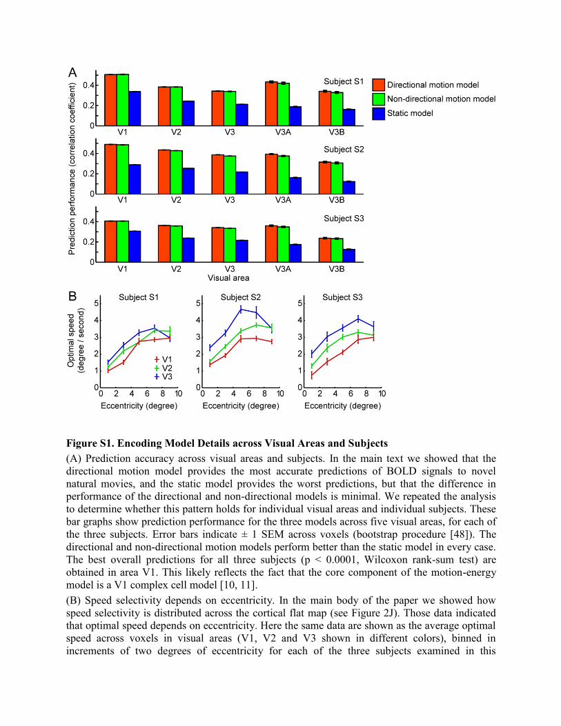
Figure S1. Encoding Model Details across Visual Areas and Subjects
(A) Prediction accuracy across visual areas and subjects. In the main text we showed that the
directional motion model provides the most accurate predictions of BOLD signals to novel
natural movies, and the static model provides the worst predictions, but that the difference in
performance of the directional and non-directional models is minimal. We repeated the analysis
to determine whether this pattern holds for individual visual areas and individual subjects. These
bar graphs show prediction performance for the three models across five visual areas, for each of
the three subjects. Error bars indicate ± 1 SEM across voxels (bootstrap procedure [48]). The
directional and non-directional motion models perform better than the static model in every case.
The best overall predictions for all three subjects (p < 0.0001, Wilcoxon rank-sum test) are
obtained in area V1. This likely reflects the fact that the core component of the motion-energy
model is a V1 complex cell model [10, 11].
(B) Speed selectivity depends on eccentricity. In the main body of the paper we showed how
speed selectivity is distributed across the cortical flat map (see Figure 2J). Those data indicated
that optimal speed depends on eccentricity. Here the same data are shown as the average optimal
speed across voxels in visual areas (V1, V2 and V3 shown in different colors), binned in
increments of two degrees of eccentricity for each of the three subjects examined in this
experiment. Optimal speed is expressed as the optimal temporal frequency divided by the
optimal spatial frequency. (Voxels for which prediction accuracy of the directional motion-
energy model was p > 0.01 or where the optimal spatial frequency was 0 cycles/degree have been
omitted.) Error bars indicate ± 1 SEM across voxels for each bin (bootstrap procedure [48]). In
all three subjects and all three visual areas there is a significant positive correlation between
eccentricity and optimal speed (p < 0.0001, t test for correlation coefficient). Because high
temporal frequency signals in natural movies have low energy, we estimated temporal frequency
selectivity only up to 4Hz. This could bias estimates of the optimal speed toward lower values,
especially for voxels in the visual periphery that are high-pass for temporal frequency (e.g.,
Figure 2G).
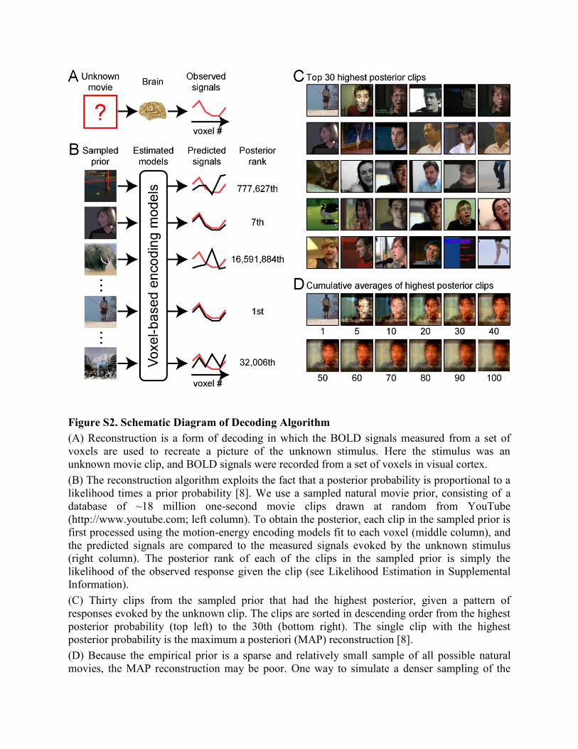
Figure S2. Schematic Diagram of Decoding Algorithm
(A) Reconstruction is a form of decoding in which the BOLD signals measured from a set of
voxels are used to recreate a picture of the unknown stimulus. Here the stimulus was an
unknown movie clip, and BOLD signals were recorded from a set of voxels in visual cortex.
(B) The reconstruction algorithm exploits the fact that a posterior probability is proportional to a
likelihood times a prior probability [8]. We use a sampled natural movie prior, consisting of a
database of ~18 million one-second movie clips drawn at random from YouTube
(http://www.youtube.com; left column). To obtain the posterior, each clip in the sampled prior is
first processed using the motion-energy encoding models fit to each voxel (middle column), and
the predicted signals are compared to the measured signals evoked by the unknown stimulus
(right column). The posterior rank of each of the clips in the sampled prior is simply the
likelihood of the observed response given the clip (see Likelihood Estimation in Supplemental
Information).
(C) Thirty clips from the sampled prior that had the highest posterior, given a pattern of
responses evoked by the unknown clip. The clips are sorted in descending order from the highest
posterior probability (top left) to the 30th (bottom right). The single clip with the highest
posterior probability is the maximum a posteriori (MAP) reconstruction [8].
(D) Because the empirical prior is a sparse and relatively small sample of all possible natural
movies, the MAP reconstruction may be poor. One way to simulate a denser sampling of the

posterior is to simply average over the clips near the peak of the posterior. Here averages over 1-
100 clips are shown. Note that to equalize the contributions from each clip we prenormalized the
pixel values of each clip to have a unit standard deviation before averaging. After averaging we
post-normalized the averaged clip so that its mean and standard deviation were equal to those of
the average of the top 100 clips. We found in practice that averaging over 100 clips near the peak
of the posterior yields robust and stable reconstructions. We call this the averaged high posterior
(AHP) reconstruction (Figure 4).
Supplemental Experimental Procedures
List of Movies Used as Stimuli
To minimize potential biases in the stimulus set, the movies used for the experiment were drawn
from a wide variety of different sources. The bulk of the movies were taken from trailers for the
following movies: “Australia”, “Bolt”, “Bride Wars”, “Changeling”, “Duplicity”, “Fuel”, “Hotel
for Dogs”, “Ink Heart”, “King Lines”, “Mall Cop”, “Madagascar 2”, “Pink Panther 2”, “Proud
American”, “Role Models”, “Shark Water”, “Star Trek”, “The Tale of Despereaux”, “Warren
Miller Higher Ground” and “Yes Man”. Additional movies were taken from following libraries:
“Artbeats HD”, “BBC Motion Gallery”, “Mammoth HD” and “The Macaulay Library”. These
movies were supplemented with high-definition movies drawn from YouTube: “IGN Game of
the Year 2008”, “JAL Boeing 747 landing Kai Tak”, “The American Recovery and
Reinvestment Plan” and “Where the hell is Matt?”.
Data Preprocessing
BOLD signals were preprocessed as described in earlier publications [8, 19]. Briefly, motion
compensation was performed using SPM '99 (http://www.fil.ion.ucl.ac.uk/spm), and
supplemented by additional custom algorithms. For each 10 minute run and each individual
voxel, drift in BOLD signals was first removed by fitting a third-degree polynomial, and signals
were then normalized to mean 0.0 and standard deviation 1.0. Retinotopic mapping data
collected from the same subjects in separate scan sessions was used to assign voxels to visual
areas [47].
To compensate for hemodynamic transients caused by movie onset, we presented 10
seconds of dummy movies before each 10 minute block. The dummy movies were identical to
the final 10 seconds of movies for each block. Data collected during this initial 10 seconds were
excluded from data analysis.
Motion-Energy Encoding Model
Our motion-energy encoding model describes BOLD signals as a linear weighted sum of local,
nonlinear motion-energy filters. The model has two main steps (see Figure 1). Movies first pass
through a bank of nonlinear motion-energy filters, and these transformed signals then pass
through a bank of temporal hemodynamic response filters. The nonlinear motion-energy filter
bank itself consists of several stages of processing (Figure 1A). To minimize the computational
burden all movie frames are first spatially down-sampled to 96x96 pixels. The RGB pixel values
are then converted into Commission internationale de l'éclairage (CIE) L*A*B* color space and
color information is discarded. The luminance patterns then pass through a bank of three-
dimensional spatiotemporal Gabor wavelet filters, where two dimensions represent space and
one represents time (see Gabor Wavelet Basis Set). The output of each quadrature pair of filters
(i.e., filters of two orthogonal phases) is squared and summed to yield local motion-energy
measurements [10, 11]. Motion-energy signals are then compressed by a log-transform and
temporally down-sampled from the original frequency of the movie (15 Hz) to the sampling rate
used to measure BOLD signals (1 Hz). Each motion-energy signal is then normalized across time
by a Z-score transformation so that each has mean 0.0 and standard deviation 1.0. Any motion-
energy signal outliers more than 3.0 standard deviations from the mean are truncated to 3.0 in
order to improve stability in the model estimation procedure. Finally, the output of each motion-
energy filter is temporally convolved with one specific hemodynamic response filter, and all
channels are summed linearly. The shape of each hemodynamic response filter is fit separately
using data from the training set (see Model Fitting). To minimize computational time we
restricted the temporal window of the hemodynamic response filters to a period 3-6 seconds (4
time samples) before BOLD signals. To simplify the association between each BOLD signal and
each one second movie clip during reconstruction we refit the encoding model after shrinking the
window so that it included only the single delay of 4 seconds (one time sample).
Note that in theory the hemodynamic convolution could be applied before down-
sampling the filtered stimuli. Although this would reproduce more faithfully the underlying
process that generates BOLD signals, it is computationally more efficient to perform the
convolution after down-sampling.
Gabor Wavelet Basis Set
One important component of the motion-energy encoding model is a bank of three-dimensional
spatiotemporal Gabor wavelet filters (Figure 1). The complete spatiotemporal Gabor wavelet
basis set contains 6,555 separate three-dimensional Gabor filters. Each filter is constructed by
multiplying a three-dimensional spatiotemporal (2 dimensions for space, 1 dimension for time)
sinusoid by a three-dimensional spatiotemporal Gaussian envelope [49, 50]. Filters occur at six
spatial frequencies (0, 2, 4, 8, 16 and 32 cycles/image), three temporal frequencies (0, 2 and 4
Hz) and eight directions (0, 45,…, 315 degrees). The zero temporal frequency filters occur at
only four orientations (0, 45, 90 and 135 degrees) and the zero spatial frequency filters occur
only once (no orientation). Filters are positioned on a square grid that covers the movie screen.
Grid spacing is determined separately for filters at each spatial frequency so that adjacent Gabor
wavelets are separated by 3.5 standard deviations of the spatial Gaussian envelope. To facilitate
the motion-energy computation [10, 11] each filter occurs at two quadratic phases (0 and 90
degrees).
Two simplified encoding models were also used in this study. The non-directional motion
model is identical to the directional model except the outputs of anti-directional filters (e.g., 0
degrees and 180 degrees) are summed at each spatial position, spatial orientation and temporal
frequency. The static model includes only the subset of filters with zero temporal frequency.
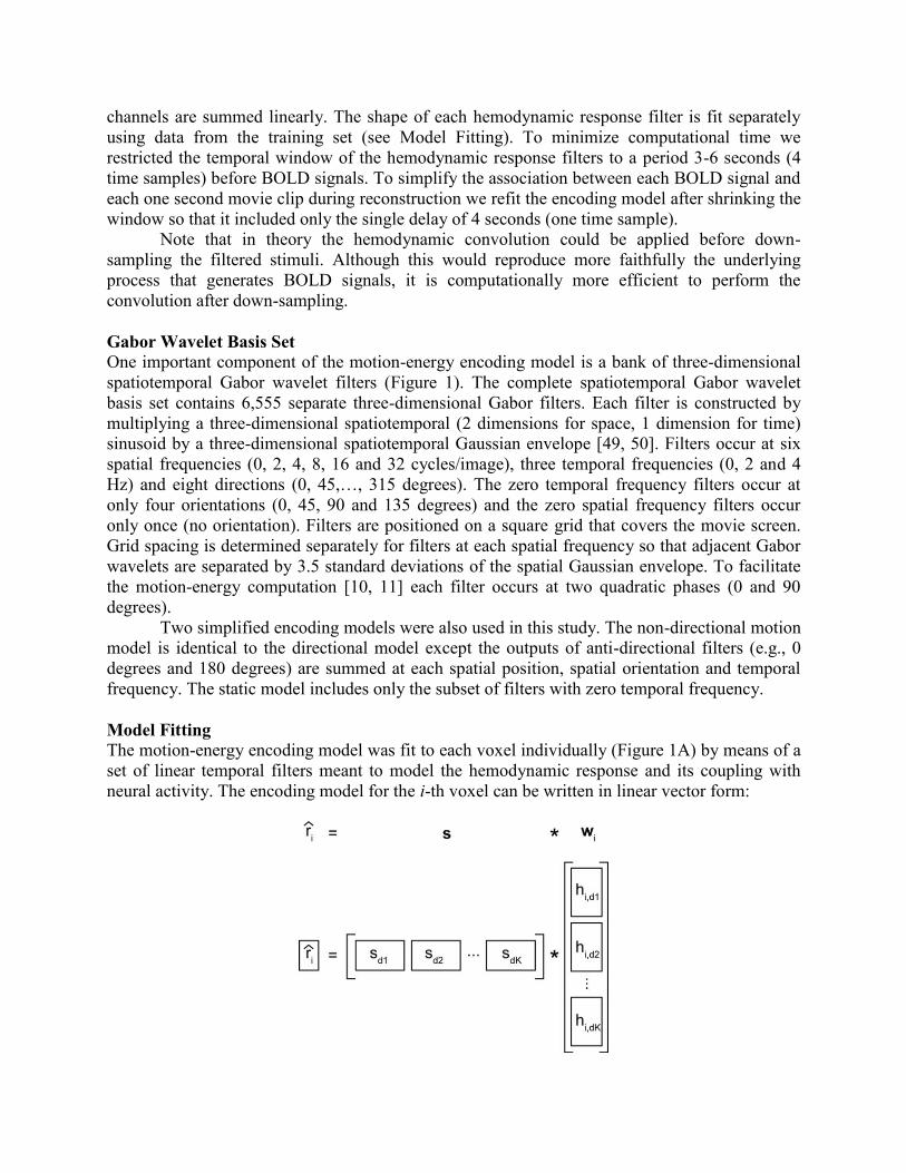
Model Fitting
The motion-energy encoding model was fit to each voxel individually (Figure 1A) by means of a
set of linear temporal filters meant to model the hemodynamic response and its coupling with
neural activity. The encoding model for the i-th voxel can be written in linear vector form:
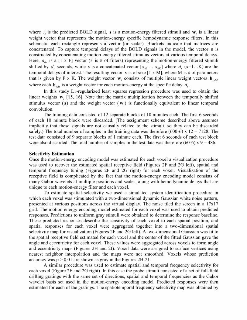
where ˆ r i is the predicted BOLD signal, s is a motion-energy filtered stimuli and wi is a linear
weight vector that represents the motion-energy specific hemodynamic response filters. In this
schematic each rectangle represents a vector (or scalar). Brackets indicate that matrices are
concatenated. To capture temporal delays of the BOLD signals in the model, the vector s is
constructed by concatenating motion-energy filtered stimulus vectors at various temporal delays.
Here, sdx is a [1 x F] vector (F is # of filters) representing the motion-energy filtered stimuli
shifted by dx seconds, while s is a concatenated vector [ sd1 … sdK] where dx (x=1…K) are the
temporal delays of interest. The resulting vector s is of size [1 x M], where M is # of parameters
that is given by F x K. The weight vector wi consists of multiple linear weight vectors hi,dx,
where each hi,dx is a weight vector for each motion-energy at the specific delay dx .
In this study L1-regularized least squares regression procedure was used to obtain the
linear weights wi [15, 16]. Note that the matrix multiplication between the temporally shifted
stimulus vector ( s) and the weight vector ( wi) is functionally equivalent to linear temporal
convolution.
The training data consisted of 12 separate blocks of 10 minutes each. The first 6 seconds
of each 10 minute block were discarded. (The assignment scheme described above assumes
implicitly that these signals are not causally related to the stimuli, so they can be discarded
safely.) The total number of samples in the training data was therefore (600-6) x 12 = 7128. The
test data consisted of 9 separate blocks of 1 minute each. The first 6 seconds of each test block
were also discarded. The total number of samples in the test data was therefore (60-6) x 9 = 486.
Selectivity Estimation
Once the motion-energy encoding model was estimated for each voxel a visualization procedure
was used to recover the estimated spatial receptive field (Figures 2F and 2G left), spatial and
temporal frequency tuning (Figures 2F and 2G right) for each voxel. Visualization of the
receptive field is complicated by the fact that the motion-energy encoding model consists of
many Gabor wavelets at multiple positions and scales, along with hemodynamic delays that are
unique to each motion-energy filter and each voxel.
To estimate spatial selectivity we used a simulated system identification procedure in
which each voxel was stimulated with a two-dimensional dynamic Gaussian white noise pattern,
presented at various positions across the virtual display. The noise tiled the screen in a 17x17
grid. The motion-energy encoding model estimated for each voxel was used to obtain predicted
responses. Predictions to uniform gray stimuli were obtained to determine the response baseline.
These predicted responses describe the sensitivity of each voxel to each spatial position, and
spatial responses for each voxel were aggregated together into a two-dimensional spatial
selectivity map for visualization (Figures 2F and 2G left). A two-dimensional Gaussian was fit to
the spatial receptive field estimated for each voxel and the center of the fitted Gaussian gave the
angle and eccentricity for each voxel. These values were aggregated across voxels to form angle
and eccentricity maps (Figures 2H and 2I). Voxel data were assigned to surface vertices using
nearest neighbor interpolation and the maps were not smoothed. Voxels whose prediction
accuracy was p > 0.01 are shown as gray in the Figures 2H-2J.
A similar procedure was used to estimate spatial and temporal frequency selectivity for
each voxel (Figure 2F and 2G right). In this case the probe stimuli consisted of a set of full-field
drifting gratings with the same set of directions, spatial and temporal frequencies as the Gabor
wavelet basis set used in the motion-energy encoding model. Predicted responses were then
estimated for each of the gratings. The spatiotemporal frequency selectivity map was obtained by
averaging predicted responses across all directions. Predictions of responses to a uniform gray
field were used to determine the response baseline.
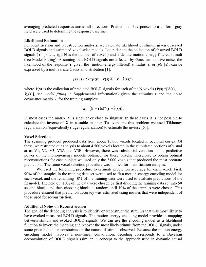
Likelihood Estimation
For identification and recostruction analysis, we calculate likelihood of stimuli given observed
BOLD signals and estimated voxel-wise models. Let r denote the collection of observed BOLD
signals ( r=[ ri, …, rN ], N is the number of voxels) and s denote motion-energy filtered stimuli
(see Model Fitting). Assuming that BOLD signals are affected by Gaussian additive noise, the
likelihood of the response r given the (motion-energy filtered) stimulus s, or p(r | s) , can be
expressed by a multivariate Gaussian distribution [1]:
p(r |s) exp{(r r (s)) 1(r r (s))'},
where ˆ r (s) is the collection of predicted BOLD signals for each of the N voxels ( ˆ r (s)=[ ˆ r i(s) , …,
ˆ r N (s)], see model fitting in Supplemental Information) given the stimulus s and the noise
covariance matrix for the training samples:
(r ˆ r (s))'(r ˆ r (s)) .
In most cases the matrix is singular or close to singular. In these cases it is not possible to
calculate the inverse of in a stable manner. To overcome this problem we used Tikhonov
regularization (equivalently ridge regularization) to estimate the inverse [51].
Voxel Selection
The scanning protocol produced data from about 15,000 voxels located in occipital cortex. Of
these, we restricted our analysis to about 4,500 voxels located in the stimulated portions of visual
areas V1, V2, V3, V3A and V3B. However, there was substantial variation in the predictive
power of the motion-energy models obtained for these voxels. Therefore, to obtain optimal
reconstructions for each subject we used only the 2,000 voxels that produced the most accurate
predictions. The same voxel selection procedure was applied for identification analysis.
We used the following procedure to estimate prediction accuracy for each voxel. First,
90% of the samples in the training data set were used to fit a motion-energy encoding model for
each voxel, and the remaining 10% of the training data were used to evaluate predictions of the
fit model. The held out 10% of the data were chosen by first dividing the training data set into 50
second blocks and then choosing blocks at random until 10% of the samples were chosen. This
procedure ensured that prediction accuracy was estimated using movies that were independent of
those used for reconstruction.
Additional Notes on Reconstruction
The goal of the decoding analysis is to identify or reconstruct the stimulus that was most likely to
have evoked measured BOLD signals. The motion-energy encoding model provides a mapping
between stimuli and evoked BOLD signals. We can use the encoding model as a likelihood
function to invert the mapping and recover the most likely stimuli from the BOLD signals, under
some prior beliefs or constraints on the nature of stimuli observed. Because the motion-energy
encoding model involves a non-linear convolution, decoding corresponds to a Bayesian
deconvolution of BOLD signals (similar in concept to the approach used in dynamic causal

modeling [52-54]). Full Bayesian deconvolution would involve a mapping between a sequence
of movie clips and a sequence of BOLD signals, which would cause a combinatorial explosion
that would make decoding much more difficult. Therefore, to simplify numerical calculation we
assume that the convolution is simply a delay in the hemodynamic response. This assumption
allows us to convert the Bayesian deconvolution problem into a simpler problem, in which the
causes of the current BOLD signal can be expressed in terms of stimuli presented at a fixed
temporal delay (here four seconds). Furthermore, this assumption allows us to decode BOLD
signals on a second by second basis, and to assess the decoding accuracy in terms of short (one
second) movie sequences.
The sampled prior used in this study consisted of many dynamic movies. However, in
some cases the movie was relatively static and did not change for many seconds (e.g., long-
lasting static scenes). In preliminary studies we found that the average high posterior (AHP)
reconstruction sometimes picked up many seconds of these static clips in a row, which visually
biased the reconstruction. To avoid choosing similar clips too many times in succession, once we
chose a clip from a single movie we discarded the subsequent five seconds of that movie from
the selection process.
In preliminary studies we also explored reconstructions in which the 100 clips with the
highest posterior probability were weighted according to their likelihood before averaging.
However, we found that the weighted average tended to be dominated by one or two clips and
the resulting reconstruction was worse than the MAP reconstruction. (This likely occurs because
the sampled movie prior is relatively sparse.) Therefore, in the current study we simply averaged
across all 100 of the clips with the highest posterior probability.
Evaluating the Accuracy of Reconstructions
To evaluate reconstruction accuracy we quantified the structural similarity between the natural
movies used as stimuli in the experiment and their reconstructions. Structural similarity was
quantified by calculating the correlation between the original movie stimuli and reconstructions
within the motion-energy feature space. Although this study is the first to assess similarity in the
motion-energy space, other studies have assessed similarity in a static complex wavelet feature
space [8, 55].
To estimate structural similarity between the test movies and the MAP reconstructions,
we first processed the test movies with the motion-energy filter bank (up to the temporal down-
sampling stage, absent the hemodynamic coupling component used in the encoding models
(Figure 1)). This produced a vector of motion-energy weights for each one second segment of the
movie. The MAP reconstructions were treated the same way, giving a vector of motion-energy
weights for each one second reconstruction. The similarity of the original movie and the MAP
reconstruction was then taken as the motion-energy domain correlation between these two
vectors, at a resolution of one second. The same procedure was applied to AHP reconstruction to
obtain structural similarity between the test movies and the AHP reconstruction. In both cases a
correlation of 1.0 indicates that the reconstruction captures all of the motion energy in the
original stimulus, while a correlation of 0.0 indicates that the reconstruction is unrelated to the
original stimulus.
To test significance of the reconstructions we compared the measured correlations to the
distribution of motion-energy filter-domain correlations between the original movies and a set of
clips drawn at random from the natural movie prior. A Wilcoxon rank-sum test was used to
examine statistical significance between the correlation values from the actual reconstructions

and those from random clips. The Wilcoxon signed-rank test was also used to determine whether
there was any significant difference in quality between MAP and AHP reconstructions. The
chance performance was shown as the 99th percentile of the null distribution (Figure 4D, dashed
line).
Supplemental References
48. Efron, B., and Tibshirani, R. (1993). An Introduction to the Bootstrap (New York: Chapman &
Hall).
49. Jones, J.P., and Palmer, L.A. (1987). An evaluation of the two-dimensional Gabor filter model of
simple receptive fields in cat striate cortex. J Neurophysiol 58, 1233-1258.
50. DeAngelis, G.C., Ohzawa, I., and Freeman, R.D. (1993). Spatiotemporal organization of simple-
cell receptive fields in the cat's striate cortex. I. General characteristics and postnatal
development. J Neurophysiol 69, 1091-1117.
51. Marquardt, D.W. (1970). Generalized Inverses, Ridge Regression, Biased Linear Estimation, and
Nonlinear Estimation. Technometrics 12, 591-612.
52. Friston, K.J., Harrison, L., and Penny, W. (2003). Dynamic causal modelling. NeuroImage 19,
1273-1302.
53. Penny, W., Ghahramani, Z., and Friston, K. (2005). Bilinear dynamical systems. Philosophical
transactions of the Royal Society of London. Series B, Biological sciences 360, 983-993.
54. Makni, S., Beckmann, C., Smith, S., and Woolrich, M. (2008). Bayesian deconvolution of fMRI
data using bilinear dynamical systems. NeuroImage 42, 1381-1396.
55. Brooks, A.C., and Pappas, T.N. (2006). Structural similarity quality metrics in a coding context:
exploring the space of realistic distortions. Proc. SPIE 6057, 299-310.