Office of the Attorney General of Florida

Charlie Crist

0.00

0.50

1.00

1.50

2.00

1st Qt r2002

2nd Qt r2002

3rd Qt r2002

4t h Qt r2002

1st Qt r2003

2nd Qt r2003

3rd Qt r2003

4t h Qt r2003

1st Qt r2004

2nd Qt r2004

3rd Qt r2004

4t h Qt r2004

RREEPPOORRTT OONN GGAASSOOLLIINNEE PPRRIICCIINNGG IINN FFLLOORRIIDDAA June 2005 Prepared by Keith B. Leffler, Ph.D. Department of Economics University of Washington and Peter K. Ashton, President Innovation and Information Consultants, Inc.

i

TABLE OF CONTENTS EXECUTIVE SUMMARY ......................................................................................................... ii

The Attorney General’s Investigation............................................................................... ii The Gasoline Price “Spike” in Spring 2004......................................................................v Summary of Findings...................................................................................................... viii

THE 2004 FLORIDA GASOLINE PRICE SPIKE.....................................................................1 SECTION 1: THE SUPPLY OF GASOLINE TO FLORIDA ....................................................1

Refining of Gasoline ..........................................................................................................1 No Gasoline Is Produced in Florida..................................................................................2 Increasing Concentration in the Refining Industry that Supplies Florida .....................3 Transportation and Wholesale Distribution of Gas to Florida........................................5 Gasoline Terminals and “Racks” in Florida.....................................................................6 Retail Marketing in Florida ..............................................................................................10 Vertical Integration of Supply in Florida ........................................................................12

SECTION 2: COSTS AND MARGINS FOR THE STAGES IN THE SUPPLY CHAIN OF GASOLINE TO FLORIDA .....................................................................................................15

Crude Oil Costs ................................................................................................................15 Refining Costs and Margins ............................................................................................20 Wholesale Distribution Costs and Margins in Florida ..................................................25 Retailing Costs and Margins in Florida ..........................................................................28 Gasoline Taxes .................................................................................................................31 High Crude Oil Costs and Refining Margins Account For the 2004 Price Spike ........33

SECTION 3: WAS THE 2004 PRICE SPIKE SPECIFIC TO FLORIDA? COMPARISONS TO PRICES IN OTHER REGIONS ........................................................................................38 SECTION 4: SUPPLY AND DEMAND ANALYSIS OF FLORIDA GASOLINE PRICES ......46

The Earnings of Integrated Petroleum Refiners ............................................................47 Overall Earnings Are Driven By Crude Oil Revenues................................................47 Earnings from Refining ................................................................................................48

Supply and Demand Factors Impacting the Refining-Shipping Margin ......................52 Gas Demand..................................................................................................................52 Gasoline Supply............................................................................................................54 Gasoline Inventories ....................................................................................................59

Regression Analysis of the Refining-Wholesaling Margin and Florida Gas Prices ...62 SECTION 5: CONCLUSIONS ...............................................................................................67

Exchange Agreements.....................................................................................................68 Gasoline Pricing and Inventories....................................................................................69

Exhibit 1: Curricula Vitae for Keith B. Leffler, Ph.D. and Mr. Peter K. Ashton

ii

EXECUTIVE SUMMARY

The Attorney General’s Investigation It is the responsibility of the Attorney General to investigate and respond to citizen

complaints regarding unexplained price hikes that could be the result of anticompetitive

behavior. In response to consumer complaints, Attorney General Charlie Crist began

voicing his concerns, as early as February 2003, about soaring fuel costs. As the price of

regular gasoline reached an average of $1.70 per gallon, the Attorney General stated:

[t]he recent spike in fuel prices is startling. I am concerned that there are those who would take advantage of the uncertain situation in the Middle East to maintain unjustifiably inflated prices. I am prepared to use the resources of this office, as well as work with the federal government, to make sure that consumers are not being exploited.

On February 18, 2003, the Attorney General sent a letter to the then Chairman of

the Federal Trade Commission, Timothy Muris, formally requesting that the Federal Trade

Commission look into the Florida market for gasoline and compare it to other markets in

the country to determine whether the recent spike in gasoline prices could be explained

by current market conditions. In response to General Crist’s letter, the Federal Trade

Commission pledged to look at the Florida market for gasoline. On February 25, 2003,

the Attorney General met individually with representatives from six major oil companies to

discuss various factors that could have caused the spike in gasoline prices. The industry

representatives stated that gasoline supplies were low due to the uncertainty in

Venezuela, the pending conflict in Iraq, and an unusually cold winter.

Soon thereafter the price of regular gasoline dropped to an average of $1.60 per

gallon. However, by summer prices began to increase again, prompting General Crist to

request the U.S. Department of Energy to assist Florida in obtaining a full explanation of

the most recent spike in gasoline prices. In a letter to Department of Energy Secretary,

Spencer Abraham, dated August 29, 2003, the Attorney General asked the Department of

Energy to direct the oil companies to provide a better explanation than the uncertainty in

Venezuela, the pending conflict in Iraq, and an unusually cold winter for the recent price

hikes for gasoline.

iii

In December 2003, Florida unleaded regular gasoline prices averaged about $1.48

per gallon. Within five months, by May 2004, the average price in Florida had increased

over 30 percent to $1.95 per gallon. While the cost of crude oil increased by about $.19

per gallon from December to May, Florida consumers were paying nearly $.50 more per

gallon at the pump. This price run-up meant that the people of Florida were paying over

$10 million more for gasoline per month at the May 2004 prices than they would have

paid had prices remained at the December 2003 level.1 Florida’s average gasoline price

increased another $.02 in June and then, after a slight decline, peaked at just under $2.00

per gallon in November 2004.

As prices continued to rise in 2004, the Attorney General continued to search for

an explanation. He invited representatives from major oil companies to Tallahassee

again to discuss rising gasoline prices. Seven oil companies accepted his invitation and

in March 2004 representatives from Amerada Hess, BP Corporation, ChevronTexaco,

Conoco-Phillips, Exxon, Marathon Ashland, and Motiva Enterprises, LLC (Shell) met with

the Attorney General. Each oil company explained that rising gasoline prices were due to

shortages caused by greater demand than supply.

At the same time, the Attorney General sought the repeal of The Motor Fuel

Marketing Prices Act (the “Act”) in the Florida Legislature. In a letter dated March 25,

2004, to Senate President Jim King and House Speaker Johnnie Byrd, General Crist

urged the Legislature to repeal the Act, which prohibits below cost fuel prices, because it

is anticompetitive. General Crist also argued that the Act was unnecessary. In his letter,

the Attorney General explained that:

[t]he antitrust laws already exist to ensure that any predatory pricing conduct on the part of a gasoline retailer will be redressed. The antitrust laws are in effect to protect competition (and therefore consumers) and my office has been, and will continue to be, vigilant in enforcing them.

After almost a year of trying to obtain a satisfactory explanation, and as consumer

frustration continued to rise over gasoline prices of more than $2.00 per gallon, General

Crist began a formal investigation. On May 25, 2004, he subpoenaed eleven oil

companies for information and records showing, among other things, the cost of

1 Based on Florida gasoline consumption from Petroleum Marketing Monthly, Tables 31 and 48.

iv

acquisition, production, inventory, wholesale prices, and retail prices for gasoline in

Florida. The subpoenas were issued to the following companies: Amerada Hess

Corporation, BP Products North America, Inc., Chevron USA. Inc., Citgo Petroleum

Corporation, Colonial Oil Industries, Inc., Conoco-Phillips Company, Exxon-Mobil

Corporation, Marathon Ashland Petroleum, LLC, Motiva Enterprises, LLC (Shell), Murphy

Oil USA, and TransMontaigne, Inc. The first subpoenas contained 29 interrogatories and

20 requests for production of documents. In response to these subpoenas, the Attorney

General’s office received approximately 153,000 pages of documents and computer discs

containing more than 44,000 files.

From this initial production, a variety of data was analyzed, including refinery

reports describing gasoline production and crude inputs, wholesale pricing data, dealer

tankwagon prices, and transportation and terminal costs. Current and historical retail

pricing data were also studied, as was refinery capacity, production, and utilization data.

Profit and loss reports for refineries were reviewed. In addition, data measuring inventory

levels and days of supply were compared to consumption.

The requests for production of documents also specifically asked for exchange

agreements, purchase agreements, sales agreements, and matched purchase/sales

agreements between companies. These agreements, which are typically used by oil

companies to acquire additional supply of gasoline in the wholesale or retail market, were

carefully reviewed by the Attorney General’s Office with the assistance of the Offices of

Attorneys General for Ohio and Pennsylvania, whose work we greatly appreciate.

Thousands of communications produced by the oil companies that discussed gasoline

inventories and sales during early 2004 were also reviewed.

During this initial document review, it was determined that additional information

was needed to understand the role of the futures market in the pricing of gasoline in the

United States. To obtain this information, General Crist served a second round of

subpoenas to many of the oil companies on October 22, 2004. These subpoenas

contained 10 interrogatories and four requests for documents and sought information and

documentation regarding each company’s participation in the oil and gas futures market

as well as its use of consultants and participation in industry and trade associations. In

response to this second round of subpoenas, the Attorney General’s office received, and

v

reviewed, approximately 83,000 pages of documents and computer discs containing more

than 15,000 files.

In December 2004, in response to an inquiry about the status of the office’s

investigation, the Attorney General said, “The people of Florida want to know why their

fuel prices are so high . . . Only by obtaining the full picture of the process by which prices

are determined can we give them a true accounting.” To aid in this effort, General Crist

retained two economists: Dr. Keith Leffler and Mr. Peter Ashton. They were asked to

analyze the data received pursuant to the subpoenas and relevant publicly available

information, to study the supply of and demand for gasoline in Florida, and to determine

as completely as possible the cause of the 2004 price spike.

Dr. Leffler is an economist with the Department of Economics, University of

Washington. He has studied the petroleum industry for over twenty-five years and

worked closely with the Florida Attorney General on an investigation of alleged gasoline

price fixing in the early 1970s. He has worked for decades with the Federal Trade

Commission and numerous state attorneys general in evaluating the economic impact on

consumers of proposed mergers of petroleum companies. Dr. Leffler has also provided

expert assistance in investigations into gasoline price spikes and high gasoline prices

conducted by the Attorneys General of Washington, Oregon, California, Arizona, and

Hawaii. Dr. Leffler’s curriculum vita is provided in Exhibit 1 to this report.

Mr. Peter Ashton is President of Innovation and Information Consultants, Inc., an

economic and financial consulting firm specializing in the economics of the petroleum

industry. Mr. Ashton has studied gasoline pricing for over twenty years as a consultant to

various states, the federal government, and private firms. Specifically, Mr. Ashton has

studied gasoline pricing issues in the states of Connecticut, Maine, Massachusetts,

Pennsylvania, West Virginia, California, Oregon, Washington, and Nevada, among

others. Mr. Ashton’s curriculum vita is also provided in Exhibit 1.

The Gasoline Price “Spike” in Spring 2004 This report examines the gasoline price increases that have occurred over the past

year and, in particular, focuses on the price increases experienced in early to mid 2004, in

an effort to determine the likely causes. In December 2003, the average price for regular

vi

gasoline in Florida was $1.48 per gallon. Over the next five months, the price average

increased by $.46, to over $1.94 per gallon in May 2004, a record high at the time.2 This

gasoline price increase was contemporaneous with record high crude oil prices.3 From

December 2003, the price of crude oil used in the Gulf Coast refineries that are the major

supply source for Florida gasoline increased by almost 20 percent to over $35.70 a barrel

in May 2004.4 The increased cost of crude oil, however, accounted for only about a third

of the $.46 per gallon increase in the price of gasoline.

Figure S-1 shows Florida retail prices as compared to the cost of crude oil.

FIGURE S-1: Florida Retail Gasoline Prices and Composite Crude Oil Prices, Monthly 2000-2004

0

50

100

150

200

250

Jan-0

0

Mar-00

May-00

Jul-0

0

Sep-00

Nov-00

Jan-0

1

Mar-01

May-01

Jul-0

1

Sep-01

Nov-01

Jan-0

2

Mar-02

May-02

Jul-0

2

Sep-02

Nov-02

Jan-0

3

Mar-03

May-03

Jul-0

3

Sep-03

Nov-03

Jan-0

4

Mar-04

May-04

Jul-0

4

Sep-04

Nov-04

Cen

ts p

er G

allo

n

Retail Crude Figure S-2 below shows the monthly difference between the retail price of gasoline in

Florida (excluding tax) and the cost of crude oil.

2 Source: Energy Information Administration’s (EIA) publication Petroleum Marketing Monthly, Table 31, various issues. (Data used is for Regular Unleaded Sales to End Users through Retail Outlets. Unless otherwise noted, this data source is used for all Retail data). 3 Adjusting for inflation, crude oil prices were higher in 1981 during the Iran-Iraq war. 4 As discussed below, the Gulf Coast refineries use a mix of crude oil from various regions. We refer to the actual mix of crude used in these refineries as a “composite” barrel.

vii

FIGURE S-2: Price Spread Between Florida Gasoline Prices and Crude Oil Cost. Monthly 2000-2004

40

50

60

70

80

90

100

110

120

130

140

Jan-

00

Mar-0

0

May-0

0

Jul-0

0

Sep-0

0

Nov-0

0

Jan-

01

Mar-0

1

May-0

1

Jul-0

1

Sep-0

1

Nov-0

1

Jan-

02

Mar-0

2

May-0

2

Jul-0

2

Sep-0

2

Nov-0

2

Jan-

03

Mar-0

3

May-0

3

Jul-0

3

Sep-0

3

Nov-0

3

Jan-

04

Mar-0

4

May-0

4

Jul-0

4

Sep-0

4

Nov-0

4

Cen

ts p

er G

allo

n

Even over the entire year of 2004, the increase in the price of gasoline in Florida is

not completely explained by the increase in the price of crude oil. In 2004, Florida

gasoline prices averaged $1.85, which is $.30 more than the $1.55 average price for

2003. But, while crude oil prices in 2004 were also substantially higher in 2004 than in

2003, the cost of crude oil used by Gulf Coast refineries increased by just $.19 per gallon.

Thus, retail gasoline price increases significantly outpaced the crude oil cost increases

during the same period.5

5 The gasoline price increases outpaced the increased price of the composite crude oil by $.11 per gallon over the year 2004. New gasoline price highs were set again in 2005. Much of the recent price surge is clearly related to the cost of crude oil. Since the previous gasoline price high in November of $2.00 per gallon, the costs of crude oil in a gallon of gasoline has increased by about $.21 per gallon. However, like the price increases of April-July 2004, the recent increases in the price of gasoline have exceeded that of the increased cost of crude oil.

viii

Summary of Findings

To examine the possible causes of the spring 2004 gasoline price spike as it

affected Florida, it was necessary to first determine where in the supply chain of gasoline

to Florida the price or cost increases occurred. After the production of crude oil, the

stages in the supply chain include: (i) the refining of gasoline from crude oil (refining), (ii)

the distribution of gasoline from refineries to storage facilities in Florida (shipping and

wholesaling), and (iii) the trucking to and sale of gasoline at retail facilities (retailing).

Prices of gasoline at each of these stages are available and allow us to identify which

stage in the supply chain primarily benefits from the price increase. The “spot price” of

gasoline is the price for gasoline purchased at the refinery gate. The “rack price”

measures the price at the next stage, the purchase of gasoline from storage facilities in

Florida that sell gasoline at wholesale for distribution to retail stations. The last stage is

the “retail price” charged to consumers by retail gas stations. By calculating the

difference between the prices at each of these stages, the gross margin earned at that

supply stage can be determined. For example, the difference between the crude oil price

and spot price is the margin or return earned at the refining stage of the supply chain.

Figure S-3 shows the prices at the different supply chain stages for the period

September 2002 through December 2004.6 The retail price shown in Figure S-3 excluded

federal, state, and local taxes of about $.48 per gallon to make the various prices

comparable. As can be seen from Figure S-3, the prices at the different stages in the

supply chain generally move together, though there are occasional compressions and

expansions of the differences in prices.

6 The composite crude price is used.

ix

FIGURE S-3: Florida Gasoline Prices at the Stages of Supply, Monthly 2000-2004 (excluding taxes)

0

20

40

60

80

100

120

140

160

Sep-02

Oct-02

Nov-02

Dec-02

Jan-03

Feb-03

Mar-03

Apr-03

May-03

Jun-03

Jul-03

Aug-03

Sep-03

Oct-03

Nov-03

Dec-03

Jan-04

Feb-04

Mar-04

Apr-04

May-04

Jun-04

Jul-04

Aug-04

Sep-04

Oct-04

Nov-04

Dec-04

Cen

ts p

er G

allo

n

Crude Rack Spot Retail

In Figure S-4, the differences between these prices at each production and distribution

stage are shown for various periods during the 2003 through 2004 period. This figure

breaks out the various components of the retail gasoline price in Florida for various time

periods, including June 2004, the peak of the spring-summer 2004 price spike and the

post-price spike period of August through December 2004. These components are the

crude oil cost, the margin earned from the refining of gasoline, the margin earned from

the wholesaling and shipping of gasoline to Florida, and the margin from the retailing of

gasoline. Figure S-4 clearly shows that there was a significant increase in the refining

margin during the gasoline price spike in the first half of 2004. Accordingly, it appears

that, in addition to the increase in the cost of crude oil, during this time, the increase in the

cost of gasoline in Florida in early 2004 was also due to an increase in refining margins,

i.e., the amount refiners received for gasoline over their crude oil costs. However, as is

also shown in Figure S-4, this refinery margin did decline significantly in the later half of

2004 to a level near that of 2003.

x

FIGURE S-4: Components of the Florida Gasoline Price

69.00

81.76

66.86

96.16

16.32

35.36

20.35

24.53

5.52

8.80

6.31

8.73

9.27

22.59

13.84

14.22

0

20

40

60

80

100

120

140

160

Dec-03 Jun-04 2003 Average Aug-Dec 2004

Cen

ts p

er G

allo

n

Crude Refining Margin Wholesale Margin Retail Margin

100.10

148.50

107.35

143.64

While the increase in crude oil prices, spot prices and refining margins for gasoline

are the principal factors behind the 2004 gasoline price increases, these factors may not

be specific to Florida. The refineries on the Gulf Coast that serve Florida also serve other

areas of the United States. (There are no refineries in Florida.) Retail and rack prices

reflect local competitive conditions. Therefore, to determine whether other factors

specifically relating to the distribution and sale of gas in Florida also contributed to the

price spike in early 2004, we compared retail and rack prices in Florida to those in other

regions. Our analysis showed that similar retail price increases and pricing patterns for

gasoline occurred throughout the area supplied by the refineries also supplying Florida.

From this finding, we conclude that the price spike in Florida in early 2004 was not due to

distribution and marketing factors specific to Florida.

Having determined that a general increase in the refining margin together with

crude oil price increases were the principal factors accounting for the increase in gasoline

prices in Florida in early 2004, we then examined the reasons for such increases at the

refining level. This examination focused on the supply and demand factors that are

xi

expected to impact gasoline prices. We found that the major factors that contributed to

the high gasoline prices in 2004 are:

• Consumer demand for gasoline - U.S. demand for gasoline has continually increased since 2000 at an annual rate of 1.7 percent. Consumption in Florida has increased by about 2.3 percent per year over the same period.

• Refinery capacity - During the same time that U.S. demand has steadily grown by 1.7 percent per year, refinery capacity has increased by only about six-tenths of one percent (.6 percent) per year. The Gulf Coast refineries which are the major suppliers to Florida have grown by about nine-tenths of one percent (.9 percent) per year over the same period.

• Refinery utilization - As a consequence of the increased supply pressure on refineries, U.S. refineries are operating at very high levels. During the period of the 2004 price spike, the Gulf Coast refineries operated at an unsustainable level of 97.6 percent of rated capacity.

• Inventories - In the petroleum “statistical region” of the United States that includes Florida,7 inventories of gasoline in the first three months of 2004, measured as days of supply, were only 79 percent of the average inventories for 2000-2003. For all of 2004, the inventories were only 83 percent of the prior three years’ average.

• Supply issues - In early 2004, there were a number of planned shutdowns of older refineries that reduced supply to Florida in a period of increasing demand, low inventories and high utilization. These included Marathon and Shell refinery closures in Texas, and Valero and Shell closures of fluid catalytic cracking units at other Texas refineries. In addition, increasingly stringent environmental rules put added pressure on supply by necessitating temporary refinery shutdowns along with higher costs.8

• Lagged response in gasoline imports - Given the increased tightness of the domestic supply of gasoline, the market relies on imports to satisfy demand. However, it takes time for international traders to respond to the profit opportunities from high U.S. prices.

Using a statistical technique called multiple regression analysis, we then examined the

relationship between these supply and demand variables and the price of gasoline and

refining margins in 2004. Specifically, we sought to determine, given the historical

relationship among these variables and gasoline prices and refining margins, whether the

7 The U.S. is divided into five regions, called Petroleum Allocation Defense Districts (PADDs), for statistical reporting purposes. Florida is in PADD I. 8 These included low gasoline sulfur requirements that took effect in 2004 and state restrictions on the use of MTBE to meet oxygenate requirements.

xii

changes in these supply and demand variables during 2004 explained the gasoline price

spike and the increased refining margin experienced in early 2004.

As a result of this analysis, we conclude that while there was an unusual gasoline

price spike in 2004, it was generally consistent with the changes in the supply and

demand variables that occurred in 2004. These changes in supply and demand variables

were clearly the primary contributor to the increase in the price of gasoline during 2004.

However, we also found in our regression analysis that the increase in refining margins

(one component of the price of gas) in early 2004 was greater than that predicted based

on past relationships between refining margins and demand and supply factors. Yet, the

particular circumstances present in early 2004 were, at the time, unique and empirical

analysis is limited to predictions based on past experience, and we cannot therefore

conclude that any artificial limits on competition lie behind the high refinery margins

earned in 2004.

The increased refining margins seen in early 2004 led to substantial increases in

domestic refining utilization. As the U.S. refineries reached their production limits, only

imported gasoline could make up for any imbalance in demand and supply. As expected

in a reasonably competitive system, increased imports of gasoline did follow in the wake

of high refining margins. In July 2004, imports of gasoline reached the second highest

level of any month during the entire period 2000-2004.9 The increased refinery utilization

and the increased importation of gasoline caused, as one would expect, refining margins

to decline and, by December 2004, refining margins were at historic and competitive

levels. Our analysis does not disprove that anticompetitive behavior such as collusion

influenced gasoline prices during 2004. However, this study does not find evidence that

such behavior has occurred or that such behavior or other anomalous behavior is needed

to explain what happened to gasoline prices.

Rather, we find that two aspects of the gasoline industry contributed significantly to

the early 2004 price spike: the high degree of interdependence among petroleum

companies and the fragile levels of gasoline inventories. Interdependence in an industry

9 The highest monthly level of imports during this period was in April 2003. These imports followed the price spike of February-March 2003. See Inquiry into August 2003 Gasoline Price Spike, Office of Oil and Gas Energy Information Administration, November 2003 and http://www.eia.doe.gov/oil_gas/petroleum/data_publications/company_level_imports/cli.html.

xiii

may lead to less aggressive price competition and the close degree of interdependence

fostered by exchange agreements in the oil industry may have provided the oil companies

a greater degree of power over prices than would be implied solely by the moderately

concentrated structure of the industry. Likewise, the decision by oil companies to

consistently maintain low inventories in order to maximize profit also made gasoline

prices more volatile. With the lack of a cushion in inventory, if demand increases beyond

expected levels and/or supply becomes tight, the response is an increase in price.

Unexpected disruptions such as refinery fires and pipeline and barge accidents only

exacerbate this sensitivity in price.

This Executive Summary of this report provides a brief chronology of the Attorney

General’s investigation and the commissioning of this study. In Section 1, we address

background information regarding the factors affecting the supply of gasoline in Florida.

We discuss the source of the gasoline, the various stages of the industry important to the

supply of gasoline to Florida consumers, and the general market structure of each of

these industry stages.

In Section 2, we then study individual supply components that make up the retail

price of a gallon of gasoline. Our goal is to identify which stage or stages of the supply

chain within the industry incurred cost or profit increases that “explain” the large price

increases of early and mid-2004. While we find that the increased cost of crude oil played

an important role in causing higher gasoline prices, we also find that the prices during the

spring-summer price spike period increased substantially more than the cost of crude oil.

These disproportionate increases resulted in petroleum refineries earning relatively high

margins. However, these high margins quickly subsided as crude oil prices continued to

increase, outpacing gasoline prices. As a result, by the last half of 2004, the average

refinery margins were in the general range of historical margins.

In Section 3, we turn to an examination of the extent to which Florida’s price

increases in early 2004 were related to events specific to Florida. We conclude that the

price increases observed in Florida during this time were in line with those incurred by

other regions subject to the same general supply factors, with no anticompetitive or

collusive factors specific to Florida being apparent.

xiv

In Section 4, we explore the profitability of the refineries supplying Florida. We find

that the profits at integrated refineries were high for a period of time in 2004. We then

explore the extent to which basic supply and demand factors lie behind these high

refinery margins and price increases of the spring-summer 2004. We find that the spring-

summer 2004 period was unusual in that the inventory levels going into the peak driving

season were quite low. The high refinery margins that ensued were essentially the result

of high demand when there was little slack in the system. We also find that in response

to the price spike, the refineries supplying Florida and the Southeast region of the United

States operated at record levels, supplying very high amounts of gasoline. In addition,

the high prices provided the incentives for increased imports which in turn lowered the

refinery margins. We conclude that these events are consistent with a reasonably

competitive market in which there are relatively few players. Based on the information we

have received and analyzed to date, we conclude that the price increases of 2004 do not

appear to be attributable to anticompetitive conduct. Section 5 is a summary of our

findings.

1

THE 2004 FLORIDA GASOLINE PRICE SPIKE

SECTION 1: THE SUPPLY OF GASOLINE TO FLORIDA

Refining of Gasoline

All gasoline sold in Florida is refined from crude oil into gasoline outside of

Florida. It is then sent to terminals and distributed by truck to various retail

gasoline outlets. Figure 1-1, from the Energy Information Administration (EIA)

provides a general description of how gasoline is manufactured and distributed to

consumers. What follows is a detailed discussion of each of these stages of

supply.10

FIGURE 1-1: Gasoline Manufacture and Distribution

The first stage of gasoline production is the supply of crude oil to

refineries. Crude oil is the principle raw material used in the production of

gasoline. Gasoline is the major product refined from crude oil. Figure 1-2 shows

the various products typically produced from a barrel of crude oil.11 About 44

percent of crude oil is refined into gasoline.

10 Source: EIA publication, “Where Does My Gasoline Come From?”, http://www.eia.doe.gov/neic/brochure/gas04/gasoline.htm. 11 Source: EIA publication, “Where Does My Gasoline Come From?”, http://www.eia.doe.gov/neic/brochure/gas04/gasoline.htm. Note that while a barrel of crude oil is 42 gallons, the yield from a barrel is over 44 gallons of product. This is because the refined products are less dense with greater average volume than the crude oil.

2

FIGURE 1-2: Average Product Yield per Barrel of Crude Oil (in Gallons)

No Gasoline Is Produced in Florida

Florida has no petroleum refineries. All gasoline consumed in Florida is

produced elsewhere and brought into Florida. The state’s gasoline is supplied

mainly by barge from domestic refineries located in Louisiana, Texas, and

Mississippi (the Gulf Coast) as well as imports from foreign refineries (the

Caribbean, South America, and Europe).12 The domestic Gulf Coast refineries

serving Florida include refineries owned by several of the major integrated

petroleum companies, such as BP, Exxon/Mobil, Chevron/Texaco, Motiva

Enterprises, LLC (Shell), Citgo, Conoco/Phillips, and Valero. In addition, Florida

is dependent on foreign imported gasoline to supply about 20 percent of its

current demand.13

According to EIA data, Hess and Colonial are the two largest importers of

gasoline into Florida. Hess imports gasoline to Florida from its Virgin Islands

refinery and provides supplies for its own retail outlets as well as other marketers

including independents. Colonial is an independent, non-integrated company

12 The majority of the U.S. refineries that supply gasoline to Florida are owned by the so-called “integrated majors.” These companies are vertically integrated and own crude oil production assets as well as refineries, transportation, storage, distribution, and frequently, retailing assets and facilities. 13 Source: EIA website: http://www.eia.doe.gov/oil_gas/petroleum/data_publications/company_level_imports/cli.html

3

that brings in supply from a variety of locations including Argentina, Italy, the

United Kingdom, and the Caribbean. It also supplies independent marketers.

Increasing Concentration in the Refining Industry that Supplies Florida The domestic Gulf Coast refineries that provide the major supply of

gasoline to Florida are located in what is known as PADD III (Petroleum

Allocation Defense District). A recent Federal Trade Commission Report on

mergers in the petroleum industry summarized the concentration of refining

capacity in PADD III.14 This data is reproduced below in Table 1-1.

TABLE 1-1: PADD III Refining Concentration Trends, Annual 1969-2003

1969 1979 1981 1985 1990 1996 2000 2001 2002 2003 4-Firm

(percent) 38.3 37.4 40.1 41.4 39.3 40.9 50.9 51.1 55.3 57.1 8-Firm

(percent) 59.7 60.0 60.8 64.4 65.0 67.3 75.6 76.6 78.2 82.6

HHI \ \ \ 681 675 721 961 976 1019 1063

Table 1-1 reports the percentage of the total refining capacity in PADD III

that is produced by the largest four and largest eight refiners. It clearly

demonstrates that refining capacity has become substantially more concentrated

in recent years. By 2003, over 82 percent of capacity was controlled by the

leading eight firms.

Table 1-1 also reports the Herfindahl-Hirschman measure of industry

concentration (HHI Index). The HHI is the standard economic measure of

concentration in an industry. The U.S. Department of Justice and the Federal

Trade Commission describe this measure as follows:

[m]arket concentration is a function of the number of firms in a market and their respective market shares…. As an aid to the interpretation of market data, the Agency will use the Herfindahl-Hirschman Index ("HHI") of market concentration. The HHI is calculated by summing the squares of the individual market shares

14 Federal Trade Commission, The Petroleum Industry: Mergers, Structural Change, and Antitrust Enforcement, Staff Report, Washington, D.C.: August 2004 (FTC Report), Table 7-7.

4

of all the participants. … The Agency divides the spectrum of market concentration as measured by the HHI into three regions that can be broadly characterized as unconcentrated (HHI below 1000), moderately concentrated (HHI between 1000 and 1800), and highly concentrated (HHI above 1800).15 As shown in Table 1-1, by 2003, refining in PADD III, the major supply

area to Florida, had become moderately concentrated with an HHI of 1063. An

HHI of 1063 can be interpreted as approximately equivalent to having 10 equal

sized suppliers.16 In contrast to a market that is controlled by two to five firms, a

market with an HHI of 1063 is one in which non-competitive cooperation is

relatively difficult to achieve.

Reliance on the 2003 concentration figure of 1063, however, is tempered

by several factors. First, this concentration measure likely overstates the actual

concentration of refinery supply to Florida because it excludes foreign refineries

that are important in supplying gasoline to Florida. Second, any such

overstatement may be offset by the fact that the concentration figure is based on

total refining capacity and not on gasoline refining capacity. Because many of

the smaller independent refineries are less complex than the larger refineries of

the integrated majors, the concentration of gasoline production in PADD III is

likely above the moderate level of 1063.

A third factor concerns the extensive use of exchange agreements among

the major refiners. Exchange agreements are contracts in which one refiner

supplies gasoline to another in one location in return for receiving gasoline at a

different location. As we discuss in detail in the Conclusion, such exchange

agreements can promote efficiencies by lowering transportation costs and

reducing capital investment costs. However, such agreements also create an

atmosphere of cooperation, making the coordination of decisions more likely.

This implies that the standard concentration measure understates the actual

15 Department of Justice/FTC Horizontal Merger Guidelines, §1.5, April 2, 1992 Revised: April 8, 1997. 16 Algebraically, the HHI equals Σ(Si)2 * 10,000, Si is the share of the ith firm. If there are N equal sized firms, the HHI equals N * (1/N)2 * 10000. Hence N = 10000/HHI.

5

likelihood of non-competitive behavior. A final factor that makes the

concentration figure less relevant with regard to the supply of gasoline to Florida

is that, unlike most other states, Florida is not subject to “clean air” rules requiring

the use of specially formulated gasoline. As a result, Florida can accept gasoline

supply from any refinery that may have a surplus, while many other states are

limited to supply from the more sophisticated refineries that can produce the

cleaner “reformulated” gasolines.17

Transportation and Wholesale Distribution of Gas to Florida

Once gasoline has been refined from crude oil, gasoline distribution and

marketing begins at the refinery "gate." The refinery gate is an industry term for

the point where finished petroleum products leave the refinery and enter the

distribution system. When finished gasoline is imported from foreign refineries,

the domestic distribution and marketing begins at the port of entry. From the

refinery or port of entry, gasoline is typically shipped in large quantities by

pipeline, tanker, or barge to distribution centers located near major consuming

areas.

There is no direct pipeline from the Gulf Coast refineries to Florida.18

Other than a limited amount of gasoline that is supplied to the Florida Panhandle

area via truck from Montgomery, Alabama and Albany, Georgia, nearly all

gasoline to Florida is supplied in bulk via barge from the Gulf Coast refineries

and via tanker from foreign refineries.19 The major Florida ports for importation of

17 Another factor implying that Florida should have relatively lower prices than other states is its freedom from dependence on MTBE. MTBE is the major additive used to meet such clean air rules. Recently MTBE has been found itself to have significant environmental issues that have led to calls for the banning of its continued use. This has led to increased cost of gasoline for areas requiring the specially formulated gasoline. Florida is, however, insulated from such cost increases. 18 The Colonial and Plantation pipelines that run from Texas to the New York area serve southern Alabama and Georgia. Spur lines run to Albany, Georgia, which is some 80 miles from Tallahassee, and to Montgomery, Alabama, which is about 140 miles from Pensacola, Florida. 19 Venezuelan and Caribbean refineries are the major non-Gulf Coast refineries supplying Florida. There are occasional shipments from West Coast refineries and Europe to Florida.

6

gasoline, both foreign and domestic, include (in order of volume) Tampa,

Jacksonville, Port Everglades, and Miami.20

Gasoline Terminals and “Racks” in Florida

After reaching the port of entry, gasoline is transferred to “terminals” which

usually consist of a set of storage tanks (“tank farms”) and loading facilities called

"racks."21 The “rack” is used for transferring gasoline from the tanks to trucks or,

occasionally, to rail cars. The gasoline is then trucked to retail gasoline stations.

There is one pipeline used to distribute gasoline in Florida, called the Central

Florida Pipeline. It runs from Tampa to Orlando, providing gasoline to the central

portion of the state.

There are two types of terminals that distribute gasoline in Florida. The first

type is a “proprietary” terminal that is owned and operated by a firm that also has

refining and marketing activities. Such a terminal is an intermediate link in that

company’s supply chain. Proprietary terminals are sometimes available to other

refiners or suppliers. For example, Chevron’s Jacksonville terminal is a

proprietary terminal but, through exchange agreements and other contractual

arrangements, other companies have access to supplies maintained at that

terminal. The second type of terminal is a “public” terminal. This is a terminal

that is owned by a company that does not refine or market gasoline. Public

terminals are generally available to any supplier meeting financial requirements.

An example of a public terminal is the Kinder-Morgan terminal in Tampa. Kinder-

Morgan is an independent, non-integrated energy company that owns and

operates many terminals.22 At its Tampa terminal, Kinder-Morgan supplies

storage, throughput, and terminal services to many other companies.

20 See Waterways Council, Florida’s Waterborne Commerce and America’s Inland Navigation System. 21 Prior to environmental concerns, the truck tank trailers were loaded from the top via nozzles that hung from a rack. Hence, the name “rack.” Today, to prevent emissions from evaporation, the trucks are loaded by sealed pipes so that there is no longer any structure at terminals resembling a rack. 22 Kinder-Morgan owns and operates the Central Florida Pipeline with a terminal at each end of the pipeline (Tampa and Orlando). It also has terminals in Jacksonville and Sarasota.

7

There are approximately 34 product terminals in Florida that store and

distribute gasoline.23 Over the last twenty years, there has been a significant

decline in the number of terminals. While data are not available specific to

Florida, Figure 1-3 shows the general trend of the number of terminals for PADD

I-C which includes Florida, Georgia, North Carolina, South Carolina, Virginia, and

West Virginia.24

FIGURE 1-3: PADD I-C Terminals, Annual 2000-2004

290 284271 261

249

2019

1918

16

0

50

100

150

200

250

300

350

2000 2001 2002 2003 2004

Wholesalers Terminal Suppliers

310303

290279

265

The graph shows that the number of terminals has declined significantly and

steadily since 2000. This is the result of several factors, including a reduction in

the level of inventories held by most companies, the impact of environmental

issues, and a trend toward joint ventures.

The segment of the petroleum industry that includes the shipment,

storage, and dissemination of gasoline at terminals is called the wholesale

segment of the industry. Because many of the same refineries providing

23 As mentioned above, terminals in Southern Alabama and Georgia also supply some gasoline to Florida. 24 Federal Trade Commission, The Petroleum Industry: Mergers, Structural Change, and Antitrust Enforcement, Staff Report, Washington, D.C.: August 2004 report, Table 9-1.

8

gasoline to Florida also own terminals and distribution facilities in Florida, the

concentration of the wholesale segment of the gasoline industry mirrors the

refining segment of the industry. Table 1-2 presents a list of the major terminals

located in Florida and indicates that the integrated majors now own over 60

percent of the terminals in Florida.

TABLE 1-2: Petroleum Product Terminals in Florida

Terminal Location

Chevron Exxon Mobil Marathon-Ashland Murphy Motiva Citgo B P H e s s Trans-

Montaigne Colonial Kinder Morgan Tota l

Jacksonville 1 1 1 1 1 5

Fort Lauderdale/Port Everglades 1 1 1 2 1 1 2 1 10

Panama City 1 1

Tampa/Port Manatee 1 1 1 2 1 1 2 1 1 11

St. Marks 1 1

Freeport 1 1

Niceville 1 1

Pensacola 1 1

Cape Canaveral 1 1

Fisher Island 1 1

Taft/Orlando 1 1

Company Total 4 1 2 3 4 3 1 3 8 3 2 34

The Lundberg Survey, Incorporated, an industry research firm, provides

annual data on market shares for gasoline sales at the wholesale level by state.

Table 1-3 summarizes the Lundberg Survey data for 2002 and 2003. The market

shares from this data indicate a moderately concentrated industry with an eight-

firm concentration ratio of about 85 percent and an HHI of slightly over 1,000.

9

TABLE 1-3: Lundberg Survey Market Share Data Summary, 2002-200325

Company 2002 2003 BP 14.08% 13.34%Chevron 8.80% 8.52%Citgo 13.98% 16.60%Conoco-Phillips 3.05% 3.21%Exxon-Mobil 13.31% 11.24%Hess 8.10% 8.55%Koch 0.79% 0.76%Marathon-Ashland 9.52% 7.58%Murphy 2.04% 2.64%Motiva Enterprises LLC (Shell) 15.03% 13.49%Sunoco 0.70% 1.71%Valero 1.00% 1.83%Colonial 2.70% 2.70%Transmontaigne 5.30% 5.30%Others 1.60% 2.53% CR4 56.40% 54.67%CR8 88.12% 84.62%HHI 1,084 1,031

In its recent study, the Federal Trade Commission confirmed the general

accuracy of these concentration statistics, reporting an HHI for the wholesaling of

gasoline in Florida of 1019 in March 2004.26 By contrast, in eight other states the

HHI is over 2000,27 and in another 24 states, it is over 1200.28 In fact, the

Federal Trade Commission data indicates that only four states have less

concentrated wholesaling of gasoline than Florida.29

In interpreting the market concentration at the wholesale level, however, it

is important to recognize the interdependencies among the major suppliers. The

25 Source: Lundberg Survey . 26 FTC Report, Table 9-6. 27 Alaska, Hawaii, Indiana, Kentucky, Michigan, Montana, North Dakota, and Ohio. 28 California, Connecticut, Delaware, Idaho, Illinois, Kansas, Louisiana, Maine, Massachusetts, Minnesota, Missouri, Nebraska, Nevada, New Jersey, New Mexico, Oklahoma, Oregon, Pennsylvania, Rhode Island, Tennessee, Utah, Washington, West Virginia, and Wyoming. 29 The four states with the lowest levels of wholesale concentration are not significantly different from Florida. These states are Iowa (HHI=910), Mississippi (960), Arkansas (975), and South Carolina (991).

10

contracts between gasoline companies, known as “exchange agreements,”

mentioned earlier, play a major role in sustaining this interdependence. Typically,

the major suppliers cannot supply all of their wholesale or retail requirements in

every region of the country in which they operate; that is, each company does not

have the refineries and/or transportation and terminal systems in all parts of the

country where it sells retail gasoline. As a result, these companies enter into

exchange agreements in which one company agrees to supply another company

in one or more locations and, in return, the second company provides supplies in

other locations to the first company.30 These exchange agreements enhance

efficiency and save costs, but, at the same time, also create and reinforce a

higher degree of interdependence among the major companies and may

enhance the effects of concentration in the industry.

Retail Marketing in Florida

From the terminal, gasoline is typically trucked to retail gasoline stations

for sale to consumers. Gasoline retailing in Florida and throughout the United

States is largely conducted through four alternative channels:

• Refiner-operated retail stations (typically called “company-operated” or co-op stations). These are stations that a refiner owns and operates. The refiner therefore controls the street price at co-op stations, and there is no “price” at which the station is supplied. In some cases, a refiner may operate stations in areas outside its own distribution system, obtaining product by exchange (or rarely by purchase) from another refiner.

• Dealer operated retail stations. These are stations that a refiner owns (or controls a lease for), and leases to a “dealer.” The dealer then operates the station and sets the price at which the gasoline is sold at retail. Dealers are required to market product branded by the refiner. The dealer purchases gasoline at the "dealer tankwagon" (DTW) price. The DTW price includes delivery into storage tanks at the station.

30 To illustrate, suppose Chevron has terminal facilities on the west coast of Florida, but none on the east coast, and BP has just the opposite. Both companies distribute gasoline throughout the state, so they enter into an exchange agreement whereby BP obtains gasoline from Chevron on the west coast of Florida and in return BP agrees to provide Chevron with gasoline from its terminal on the east coast. Each company saves transportation costs as well as eliminates the need to build redundant facilities.

11

• Jobber supplied stations. Refiners frequently enter into arrangements with distributors called jobbers who pick up branded or unbranded gasoline from a terminal. The jobber then can supply stations that it owns and operates, stations at which it has established its own dealers, or stations owned and operated by an independent entrepreneur. Jobbers buy gasoline at the “rack” price. The rack price does not include the cost of transporting the gasoline from the terminal to the retail stations. Most branded and some unbranded jobbers will have contracts with their suppliers that provide some assurance of product availability.

• Independent retailers. This is a fast growing method of marketing gasoline in which retailers purchase gasoline directly from refiners (at the rack, or in some cases, in bulk) for resale to consumers at their own retail outlets. Independent retailers include convenience stores (e.g., Circle K), high volume independent gasoline retailers (e.g., Racetrack), and discount mass merchandisers (e.g., Costco). These marketers sell “unbranded” gasoline.31

There are over 9,000 gasoline stations serving Florida consumers.32 In

Florida, about 77 percent of gasoline is distributed at the rack to jobbers and/or

independent retailers, 21 percent is distributed through company or dealer

stations, and about two percent through bulk sales.33 Nationwide, about 67

percent is distributed through rack sales, 20 percent through company or dealer

stations, with about 13 percent through bulk sales. In contrast, on the West

Coast of United States (PADD V) over 55 percent of gasoline is distributed

through company or dealer stations and only about 35 percent through rack

sales.34 These differences are potentially significant and important to

understanding competitive differences across regions.

31 That is, the gasoline is not identified with any particular refiner. 32 FTC Report, Table 9. 33 EIA, Petroleum Marketing Annual, 2003, Table 43. 34 The EIA notes that “[t]he share of gasoline sold through each of the major channels, and at each price level, represents a significant difference between regional gasoline markets in various parts of the United States….The share of refiner sales made through company operated retail outlets is fairly consistent across regions, and bulk sales represent a relatively small portion of refiner sales except in Petroleum Administration for Defense District (PADD) III, the Gulf Coast. The largest deviation between regions is in the relationship between rack and DTW sales. Rack sales range from as little as 18 percent of refiner gasoline sales in California, to 70 percent in the Midwest (PADD II). Conversely, DTW, which represents 53 percent of refiner sales in California, makes up only two percent of PADD III gasoline sales.” Inquiry into August 2003 Gasoline Price Spike, Office of Oil and Gas Energy Information Administration, November 2003 (EIA Report), at 48.

12

Brand level concentration measured at retail in Florida is very similar to

concentration levels found for refining and for wholesaling. According to the FTC

Report, the HHI calculated from brand sales in Florida was 1,022 for the year

2002.35

A growing phenomenon impacting the retailing of gasoline is the

emergence of “hypermarketers.” Hypermarketers are large retailers of general

merchandise and grocery items, such as grocery supermarkets, mass

merchandisers, and club stores. According to the Federal Trade Commission;

[t]he success of the larger hypermarkets stems from the fact that they sell significantly higher volumes of gasoline at lower prices than their competitors. One reason hypermarkets can under-price more traditional retailers is that the costs associated with constructing and operating hypermarket sites are considerably lower than those of other gasoline retailers. In addition to enjoying lower construction and operating costs, hypermarketers may be willing to sell gasoline at smaller margins as part of a loss-leader or similar marketing strategy.36 Florida has shown a significant growth of retail gasoline sales by

independent “hypermarketers.” These are sales by large retailers that have

begun to branch into selling gasoline. Such sellers tend to be very price-

competitive, pressuring other sellers to maintain low prices. These sellers seek

out the most favorable buying prices and have relatively lower costs of

marketing. The latest data available (March 2002) indicates that Florida had the

largest percentage of such sales of any state in PADD I.37

Vertical Integration of Supply in Florida

Many of the primary suppliers of gasoline into Florida, including BP,

Motiva Enterprises, LLC (Shell), Citgo, Marathon-Ashland, ExxonMobil, and

Chevron are vertically integrated petroleum companies. This means that they

typically own rights to crude oil, the refineries that produce the gasoline sold in 35 FTC Report Table 9-7. Of course, there is not a statewide relevant economic market for the sale of gasoline to consumers, but rather many local markets. The concentrations within the local markets likely range above and below the state average. 36 FTC Report, at 239. 37 FTC Report, Table 9-9.

13

Florida, many of the terminals and distribution facilities that supply gas to Florida,

and the retail outlets that sell their branded gasoline to Florida consumers. The

overall economic impact of substantial vertical integration in any industry is

unclear. On one hand, vertical integration can result in efficiencies and cost

savings which can result in lower prices to consumers.38 However, in some

circumstances, a high degree of vertical integration may have anticompetitive

impact by raising the cost of entry to non-integrated potential rivals because the

vertical integration can reduce the supply options available to those potential

competitors, in this case independent oil companies with no control of crude oil or

refineries.

Vertically integrated firms control the supply of gasoline that flows through

their chain of distribution. In a market where supply is controlled by a small

number of such integrated firms, those firms, through oligopolistic coordination,

may be able to charge high wholesale prices absent the entry threat of an

independent wholesaler. In addition, by controlling a substantial percentage of

retail outlets, through both company-operated stations and dealer-stations, the

vertical integration may aid in cooperation by making pricing decisions more

transparent. Vertically integrated refiner-marketers may also exercise control

over retail prices which is disproportionate to their retail presence. This can

occur because the integrated suppliers represent the threat of a price squeeze

whereby they can charge high wholesale prices and low retail prices, placing

independent marketers in an unprofitable situation. 39 In addition, the integrated

firms’ potential to control supply of unbranded wholesale gasoline may result in

higher average product costs to the non-integrated marketers, especially in times

of rapidly increasing prices due to “scarce supply.” With tight supply, the

38 See, Carlton and Perloff, Modern Industrial Organization, for a discussion of the types of efficiencies that can occur from vertical integration. 39 This will depend on balancing the effects of vertical integration on the demand for wholesale gasoline and the incentives to raise rivals costs. See, Richard Gilbert and Justine Hastings, “Vertical Integration in Gasoline Supply: An Empirical Test of Raising Rivals’ Costs,” Program on Workable Energy Regulation, University of California Energy Institute, PWP-084, July 2001.

14

integrated companies have an incentive to favor their own dealers, supplying

independent marketers only if product is available.40

Economic studies have confirmed that a high degree of vertical integration

can affect wholesale prices. Professors Richard Gilbert and Justine Hastings in

a study of the effect of the Tosco-Unocal merger on gasoline prices in California

found “evidence that vertical integration matters for upstream retail prices and

that wholesale prices tend to be higher in markets with large vertically integrated

firms. This finding is consistent with the strategic incentive and ability of vertically

integrated firms to raise input costs to downstream rivals.41 The same study also

found that unbranded wholesale (rack) prices tended to be higher in markets

where integrated firms had higher market shares. In another study, Professor

Hastings found that when independent marketers left the market, competitors

responded by increasing prices.42 Of significance to this report, when price

spikes occur, it is typically the unbranded wholesale (rack) price that is elevated

first (and to a higher level) than branded wholesale prices. Also, the typical lag

between the increase in rack prices and the increase in street prices puts further

pressure on independent marketers during times of price spikes.

The existence of independent marketers in both the wholesale and retail

segments of the industry are therefore important competitive constraints on the

behavior of the integrated major petroleum companies. However, it does not

appear that this is as significant an issue in Florida as elsewhere given that the

overall level of concentration in the wholesaling of gasoline is relatively low in

Florida.43

40 For example, Exxon-Mobil stopped selling unbranded rack gasoline in Florida in November 2003, thereby eliminating a source of supply for independent gasoline marketers. The phenomenon of “favoring” owned stations in times of scarcity is manifested by DTW prices tending to lag rack prices when prices are rising. 41 Gilbert and Hastings, note 42. 42 Justine Hastings, “Vertical Relationships and Competition in Retail Gasoline Markets, Empirical Evidence from Contract Changes in Southern California,” http://www.nber.org/~confer/2002/iow02/hastings.pdf. 43 The FTC study reports that, “[t]he increase in scale of operations in the petroleum industry has not been accompanied by an increase in vertical integration. Rather, vertical integration between crude oil production and refining has tended to decline for the major oil companies. The incentives for vertical integration have diminished as refineries have become more flexible in the

15

SECTION 2: COSTS AND MARGINS FOR THE STAGES IN THE SUPPLY CHAIN OF GASOLINE TO FLORIDA

As explained in Section 1, the supply of gasoline to Florida involves a

number of stages. Crude oil must be supplied to the Gulf Coast and other

refineries that produce gasoline, the refined gasoline must then be shipped to

Florida, where it is held in terminals for delivery to retail gasoline stations, and

finally the gasoline must be sold at retail to consumers. Costs must be recovered

and reasonable economic profit must be earned at each of these stages to

motivate continued supply. The competitive retail price can be broken into the

following component competitive costs: crude oil supply, refining, wholesale

shipping and distribution, trucking to stations, and retailing.

In this section, we examine each of these component parts of the Florida

gasoline prices with an emphasis on which segments of the industry profited the

most from the high prices paid by Florida consumers for gasoline in the spring-

summer of 2004.

Crude Oil Costs

Gasoline supply begins with the production and transportation of crude oil

to refineries. The Gulf Coast refineries that supply the majority of the gasoline

sold in Florida obtain crude oil from domestic wells in Texas, Louisiana,

Oklahoma and Mississippi, and from foreign imports. Figure 2-1 shows the

sources and percentages of supply of crude oil to PADD III refineries and

illustrates that much of PADD III crude oil input is produced domestically.44

types of crude oil that they can process. The development of spot and future markets also has reduced the risks of acquiring crude oil through market transactions compared to relying upon vertical integration and intra-company transfers. Several significant refiners including Valero/UDS, Sunoco, Tesoro, and Premcor - have no crude oil production, and integrated petroleum companies today tend to depend less on their own crude oil production. Nationally, the share of gasoline distributed by jobbers increased from 55% to 61% between 1994 (the earliest year for which data are available) and 2002. Thus, refiners have sold an increasing share of gasoline at the terminal and a declining share at stations that they own or to which they deliver.” FTC Report at 10-11. 44 Source: EIA, Petroleum Supply Monthly – Tables 26, 28, and 43, various months.

16

FIGURE 2-1: PADD III Sources of Crude Oil, 2004

Domestic, 40.4%

Saudi Arabia, 7.8%

Iraq, 3.7%Venezuela, 9.9%

Nigeria, 4.7%

Mexico, 12.9%

Persian Gulf, 13.3%

Other OPEC, 3.2%

Other non OPEC, 7.2%

Different crude oils from various locales have different chemical

characteristics. The most important differences in the characteristics are those

relating to the density (viscosity) of the crude (heavy or light) and the sulfur

content (low sulfur is called sweet crude while high sulfur is called sour crude).

Heavy, sour crude oil generally sells at a lower price than light, sweet crude oil

because it yields less of the “light” (more valuable) refined products (such as

gasoline, diesel, and jet fuel) and is more expensive to refine.45 While individual

refineries are usually designed in anticipation of a particular type of crude oil

input, refineries can and do substitute among the available crude oils depending

upon their relative prices. Such substitution allows refineries to maximize the

value added from the refining process. The ability of refineries to substitute

among crude oils of different characteristics in response to changing crude oil

price differentials results in long run parity relationships among the prices of

crude oils. 45 FTC Report, page 4.

17

The major types of crude oils used in the Gulf Coast refineries (PADD III)

include light sweet crude oil exemplified by West Texas Intermediate crude oil

(WTI), light sour crude exemplified by Louisiana Island Eugene crude, and heavy

crude exemplified by Mexican Maya crude. Figure 2-2 shows the prices of these

crude oils along with a “composite” of these as a proxy of the overall level of

crude oil used by Gulf Coast refineries for the period 2000-2004.46

FIGURE 2-2: Crude Oil Prices, Monthly 2000-2004

0

20

40

60

80

100

120

140

Jan-0

0

Mar-00

May-00

Jul-0

0

Sep-00

Nov-00

Jan-0

1

Mar-01

May-01

Jul-0

1

Sep-01

Nov-01

Jan-0

2

Mar-02

May-02

Jul-0

2

Sep-02

Nov-02

Jan-0

3

Mar-03

May-03

Jul-0

3

Sep-03

Nov-03

Jan-0

4

Mar-04

May-04

Jul-0

4

Sep-04

Nov-04

Cen

ts p

er G

allo

n

WTI Eugene Island Maya Heavy Composite

Figure 2-3 shows the costs of the Gulf Coast composite crude oil along

with the prices of New York Mercantile (NYMEX) crude oil and Alaska North

Slope (ANS) crude oil.47

46 Source: EIA, Petroleum Marketing Monthly – Table 22, various months, Platt’s Oilgram Price Report. Dollars per barrel were converted to cents per gallon based on 42 gallons per barrel of crude oil. The composite is calculated weighting WTI by 25%, Eugene Island by 40%, and Maya by 35%. 47 Sources: EIA, Petroleum Marketing Monthly – Table 22, various months and http://www.eia.doe.gov/emeu/international/crude2.html. NYMEX is the New York Mercantile Exchange where current and futures contracts, including imported crude oil, are bought and sold. ANS crude oil supplies the west coast PADD V refineries and some Far East refineries.

18

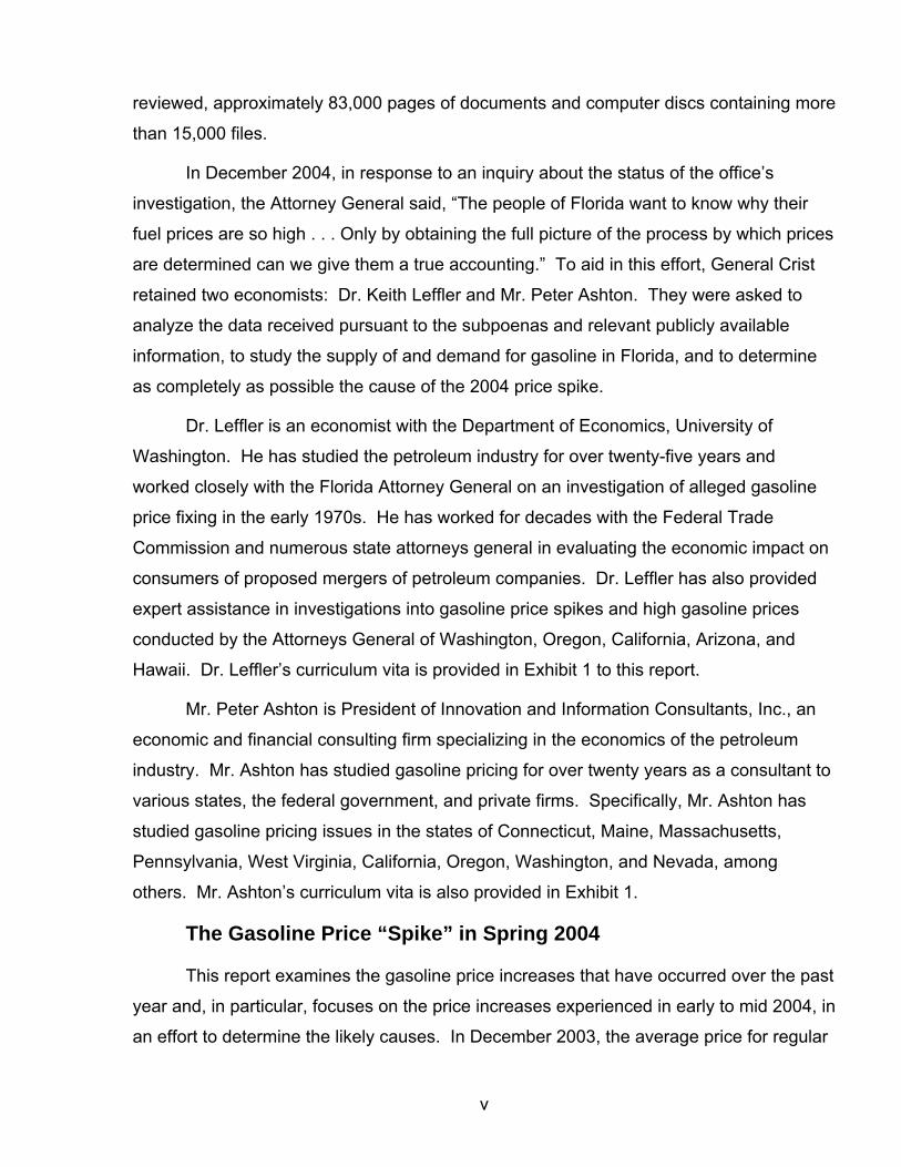
FIGURE 2-3: Gulf Coast Composite, NYMEX, and ANS Crude Oil Price, Monthly 2000-2004

0

20

40

60

80

100

120

140

Jan-0

0

Mar-00

May-00

Jul-0

0

Sep-00

Nov-00

Jan-0

1

Mar-01

May-01

Jul-0

1

Sep-01

Nov-01

Jan-0

2

Mar-02

May-02

Jul-0

2

Sep-02

Nov-02

Jan-0

3

Mar-03

May-03

Jul-0

3

Sep-03

Nov-03

Jan-0

4

Mar-04

May-04

Jul-0

4

Sep-04

Nov-04

Cen

ts p

er G

allo

n

Composite NYMEX ANS The figure shows the close relationships between the prices of these crude oils.

The correlation coefficients between both the composite and NYMEX crude oil

price series and the composite and ANS crude oil price series is .9855. Both

correlations are statistically significant at the one percent level.

Figure 2-3, shows that the composite crude oil costs had a temporary

peak in the fall of 2000 of about $.73 per gallon. The price then drifted down to a

low of about $.40 per gallon by the end of winter of 2001. From there, the prices

generally trended upwards (with a transitory peak in February 2003),48 reaching

the mid to upper seventies by the beginning of 2004. From that point, crude oil

prices climbed to an all time, nominal historic high of $1.086 per gallon in

October 2004. Given the $.35 plus increase in crude oil costs during 2004, it

certainly is no surprise that retail gasoline prices also had substantial increases

during the year.

48 For details on this transitory peak, see, EIA report, Inquiry Into August 2003 Gasoline Price Spike, November 2003.

19

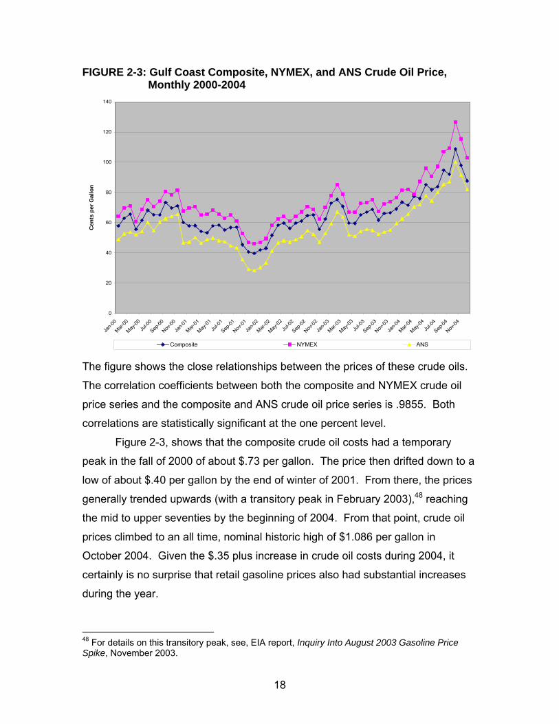
Figure 2-4 shows the WTI crude oil prices for the period 1980 through

2004, converting the crude oil prices to “real” 2004 prices.49

FIGURE 2-4: Inflation Adjusted WTI Crude Oil Price, Annual 1980-2004

0

20

40

60

80

100

120

140

160

1980

1981

1982

1983

1984

1985

1986

1987

1988

1989

1990

1991

1992

1993

1994

1995

1996

1997

1998

1999

2000

2001

2002

2003

2004

Cen

ts p

er G

allo

n

This figure shows that while crude oil prices were relatively high in 2004

compared to the recent past these “high” crude oil prices were substantially lower

than those seen in the early 1980’s. Also, contemporaneous with current retail

gasoline prices that are substantially higher than those during the price spike of

spring-summer 2004, crude oil prices have recently increased to new highs after

the temporary declines of late 2004 and early 2005. An all time high crude price

(at the time this section was prepared) of $1.36 per gallon ($57.27 per barrel)

was reached on April 1, 2005.50

49 We report WTI prices in this figure since we do not have a price series for the Maya crude oil for the 1980s. Sources: EIA, Petroleum Marketing Monthly, Table 21 and http://www.eia.doe.gov/emeu/aer/txt/ptb0518.html. 50 Source: http://www.latimes.com/business/la-fi-gas5apr05,1,606976.story?coll=la-headlines-business.

20

Refining Costs and Margins The next stage in the supply of gasoline to Florida is the refining of crude

oil into gasoline. This component of the gasoline price is measured by the gross

margin obtained by the petroleum refineries supplying Florida. The overall gross

margin earned by a petroleum refinery is the difference between the revenue

received from refined product less the cost of the crude oil used to make the

refined product. Because this report focuses on gasoline prices, we define the

per gallon refinery gasoline gross margin as the difference between (i) the value

of gasoline at the refinery, which is given by the “spot” price of gasoline, and (ii)

the cost per gallon of crude oil. We use the Gulf Coast gasoline spot price as the

measure of the value of gasoline at the refinery gate because the majority of

gasoline sold in Florida comes from Gulf Coast refineries.

Even this simplified measure of the gasoline refinery margin presents

definitional issues since there are different prices for different grades of gasoline,

e.g., regular, mid-grade and premium, and for different types of gasoline, e.g.,

conventional and reformulated gasoline. However, as shown in Figures 2-5 and

2-6 the prices of the various grades and types of gasoline are very closely related

to one another.51

51 Sources: EIA, Petroleum Marketing Monthly, Tables 31, 32, and 34, various months. Data for Conventional and Reformulated gasoline is for PADD I, rather than for Florida since reformulated gasoline is not sold in Florida. The correlation coefficient between Regular and Premium is .9987; and between conventional and reformulated regular gasoline is .9787.

21

FIGURE 2-5: Florida Average Retail Prices by Grade, Monthly 2000-2004

0

20

40

60

80

100

120

140

160

180

200

Jan-0

0

Mar-00

May-00

Jul-0

0

Sep-00

Nov-00

Jan-0

1

Mar-01

May-01

Jul-0

1

Sep-01

Nov-01

Jan-0

2

Mar-02

May-02

Jul-0

2

Sep-02

Nov-02

Jan-0

3

Mar-03

May-03

Jul-0

3

Sep-03

Nov-03

Jan-0

4

Mar-04

May-04

Jul-0

4

Sep-04

Nov-04

Cen

ts p

er G

allo

n

Midgrade Premium Regular FIGURE 2-6: PADD I Average Retail Prices by Formulation,

Monthly 2000-2004

0

20

40

60

80

100

120

140

160

180

Jan-0

0

Mar-00

May-00

Jul-0

0

Sep-00

Nov-00

Jan-0

1

Mar-01

May-01

Jul-0

1

Sep-01

Nov-01

Jan-0

2

Mar-02

May-02

Jul-0

2

Sep-02

Nov-02

Jan-0

3

Mar-03

May-03

Jul-0

3

Sep-03

Nov-03

Jan-0

4

Mar-04

May-04

Jul-0

4

Sep-04

Nov-04

Cen

ts p

er G

allo

n

Conventional Reformulated

22

For simplicity, we can therefore focus on the spot price of regular conventional

gasoline to illustrate the patterns over time in the gasoline gross margins for

petroleum refineries. This gasoline spot price is particularly relevant since

regular is the dominant grade of gasoline in Florida and Florida does not use

reformulated gasoline.52

Figure 2-7 charts the monthly refinery gasoline gross margin (as defined above)

for the period 2000 – 2004.53 The refinery margin is generally in the range of

$.10 - $.30 per gallon. However, there are two obvious “spikes” in this margin

that occurred in April 2001 and in May 2004. Figure 2-8 highlights these refining

margin anomalies by focusing separately on each year 2000 – 2004.

FIGURE 2-7: Gulf Coast Gross Refinery Margin, Monthly 2000-2004

0

10

20

30

40

50

60

Jan-0

0

Mar-00

May-00

Jul-0

0

Sep-00

Nov-00

Jan-0

1

Mar-01

May-01

Jul-0

1

Sep-01

Nov-01

Jan-0

2

Mar-02

May-02

Jul-0

2

Sep-02

Nov-02

Jan-0

3

Mar-03

May-03

Jul-0

3

Sep-03

Nov-03

Jan-0

4

Mar-04

May-04

Jul-0

4

Sep-04

Nov-04

Cen

ts p

er G

allo

n

52 Regular constitutes approximately 70 percent of gasoline sold in Florida. Source: EIA, Petroleum Marketing Monthly – Table 43, various months. Table 34 in the same publication shows that no reformulated gasoline was sold in Florida during this period. 53 Sources: EIA, Petroleum Marketing Monthly, Table 22, various months; http://www.eia.doe.gov/neic/historic/hpetroleum2.htm - link: Gasoline Spot.

23

FIGURE 2-8: Gulf Coast Gross Refining Margins by Year, Monthly 2000-2004

0

10

20

30

40

50

60

Jan Feb Mar Apr May Jun Jul Aug Sep Oct Nov Dec

Cen

ts p

er G

allo

n

2000 2001 2002 2003 2004 Figure 2-9 shows the average annual refining margins for each year 2000

through 2003, with 2004 divided into relevant periods.54

FIGURE 2-9: Average Gulf Coast Refining Margins, by Relevant Period 2000-2004

18.721.1

15.2

20.3

29.2

40.6

24.5

0

5

10

15

20

25

30

35

40

45

2000 2001 2002 2003 Jan-Mar 2004 Apr-Jul 2004 Aug-Dec 2004

Cen

ts p

er G

allo

n

54 The average of $.263 per gallon for 2004 does not include the spike period.

24

The average margin over the entire 2000 - 2004 period is $.213 per gallon.55

However, the price spike period of 2004 resulted in unusually high refining

margins of over $.40 per gallon, almost double the average.

Even though gasoline prices reached a peak for the year 2004 in

November, the refining margins during the latter part of 2004 (August -

December) are only somewhat above those of 2003. By December 2004, the

margin was only $.157 per gallon which was about $.03 per gallon below the

average for 2000-2003.

In addition to examining the refining margins for the Gulf Coast refineries

we have also examined refining margins based on New York Harbor and Los

Angeles prices.56

FIGURE 2-10: Gulf Coast, New York, and Los Angeles Gross Refinery Margins, Monthly 2000-2004

0

10

20

30

40

50

60

70

80

Jan-0

0

Mar-00

May-00

Jul-0

0

Sep-00

Nov-00

Jan-0

1

Mar-01

May-01

Jul-0

1

Sep-01

Nov-01

Jan-0

2

Mar-02

May-02

Jul-0

2

Sep-02

Nov-02

Jan-0

3

Mar-03

May-03

Jul-0

3

Sep-03

Nov-03

Jan-0

4

Mar-04

May-04

Jul-0

4

Sep-04

Nov-04

Cen

ts p

er G

allo

n

Gulf Coast New York Los Angeles

55 The average of $.213 per gallon includes the price spike period (April – July 2004). Eliminating the price spike period from our average, results in an average refining margin over the 2000 – 2004 period of $.199 per gallon. 56 Sources: EIA, Petroleum Marketing Monthly, Table 22, various months; http://www.eia.doe.gov/neic/historic/hpetroleum2.htm - link: Gasoline Spot.

25

Figure 2-10 shows that the refinery margins based on New York prices are nearly

identical to those in the Gulf Coast (correlation coefficient = .9446). However,

margins for Los Angeles refineries are both higher (average margin 2000 - 2003

= $.2996 per gallon as compared to $.1885 per gallon for Gulf Coast) and

relatively independent (correlation coefficient = .8012). The relative

independence of these margins is not surprising given the physical separation of

these supply regions. The very high margins in Los Angeles do suggest

substantial supply issues on the West Coast of the United States that have not

affected Florida.

Wholesale Distribution Costs and Margins in Florida The next stage of production in the supply of gasoline to Florida is the

shipping of product to terminals for distribution to Florida retail gasoline stations.

This “wholesale” margin is simply the difference between the price of the

gasoline at the refinery (the “spot” price) and the price of the gasoline when it is

sold at a terminal in Florida (the “rack” price). We again use the U.S. Gulf Coast

spot price as the measure of the price at the refinery.

There are currently 34 different terminals in Florida.57 At each terminal

there can be many prices as each petroleum company using the terminal may

quote its own prices. We have summarized the many rack prices by taking the

average of the BP Oil and the Chevron (branded) regular unleaded rack prices at

the Panama City and the Miami terminals. We have confirmed that this resulting

average price is highly correlated with the prices of other suppliers and the prices

at other terminals.58 This is demonstrated by Figures 2-11 and 2-12.59 Figure 2-

11 shows the average branded regular unleaded rack prices for Jacksonville, 57 As mentioned in note 26, terminals in Southern Alabama and Georgia also supply some gasoline to Florida. 58 Correlation coefficients between the brands (for branded, regular unleaded gasoline) range from .9982 to .9998 – almost perfectly correlated. Correlation coefficients between the mentioned cities (also for branded, regular unleaded gasoline) range from .9965 to .9998 – again, almost perfect correlations. 59 Source: DTN FastRacks data obtained by Florida AG’s office. This DTN data is electronically gathered for each supplier’s prices and products at 1,200 terminals in 360 cities in the U.S. and Canada. These figures begin in September 2002 because this was the earliest date for which we received consistent DTN data. Monthly average price by brand uses all cities, and averages the daily prices for branded, regular unleaded gasoline. Monthly average price by city uses all suppliers and averages the daily price for branded, regular unleaded gasoline.

26

Miami, Orlando, Panama City, Pensacola, and Tampa for the period September

2002 through December 2004.

FIGURE 2-11: Average Rack Price by City, Monthly Sept. 2002 – Dec. 2004

0

20

40

60

80

100

120

140

160

Sep-0

2

Oct-02

Nov-0

2

Dec-0

2

Jan-

03

Feb-0

3

Mar-0

3

Apr-0

3

May-0

3

Jun-

03

Jul-0

3

Aug-0

3

Sep-0

3

Oct-03

Nov-0

3

Dec-0

3

Jan-

04

Feb-

04

Mar-0

4

Apr-0

4

May-0

4

Jun-

04

Jul-0

4

Aug-0

4

Sep-0

4

Oct-04

Nov-0

4

Dec-0

4

Cen

ts p

er G

allo

n

Tampa Pensacola Panama City Orlando Miami Jacksonville Figure 2-12 shows the average branded regular unleaded price for BP, Chevron,

Citgo, Conoco, Marathon and Shell from September 2002 through December

2004.

FIGURE 2-12: Average Rack Price by Brand, Monthly Sept. 2002-Dec. 2004

0

20

40

60

80

100

120

140

160

Sep-0

2

Oct-02

Nov-0

2

Dec-0

2

Jan-

03

Feb-0

3

Mar-0

3

Apr-0

3

May-0

3

Jun-

03

Jul-0

3

Aug-0

3

Sep-0

3

Oct-03

Nov-0

3

Dec-0

3

Jan-

04

Feb-

04

Mar-0

4

Apr-0

4

May-0

4

Jun-

04

Jul-0

4

Aug-0

4

Sep-0

4

Oct-04

Nov-0

4

Dec-0

4

Cen

ts p

er G

allo

n

BP Chevron Citgo Conoco Marathon Shell

27

Figure 2-13 charts the monthly gasoline wholesale margins, as defined

above, for gasoline supplied to Florida for the period September 2002 through

2004.60

FIGURE 2-13: Florida Gross Wholesale Margin, Monthly Sept. 2002 - Dec. 2004

0

2

4

6

8

10

12

14

16

18

Sep-02

Oct-02

Nov-02

Dec-02

Jan-0

3

Feb-03

Mar-03

Apr-03

May-03

Jun-0

3Ju

l-03

Aug-03

Sep-03

Oct-03

Nov-03

Dec-03

Jan-0

4

Feb-04

Mar-04

Apr-04

May-04

Jun-0

4Ju

l-04

Aug-04

Sep-04

Oct-04

Nov-04

Dec-04

Cen

ts p

er G

allo

n

The wholesale margin generally moves between $.04 and $.09. Figure 2-

14 gives the wholesale margin for the intervals September, 2002 – November,

2003, December, 2003 – March, 2004, April – July, 2004, and August, 2004 –

December, 2004.

60 Sources: http://www.eia.doe.gov/neic/historic/hpetroleum2.htm - link: Gasoline Spot. Rack prices are from DTN as described above.

28

FIGURE 2-14: Florida Gross Wholesale Margin, by Relevant Period Sept. 2002-Dec. 2004

6.495.81

6.54

8.73

0

1

2

3

4

5

6

7

8

9

10

Sep 02 - Nov 03 Dec 03 - Mar 04 Apr 04 - Jul 04 Aug 04 - Dec 04

Cen

ts p

er G

allo

n

The average margin in the September 2002 - March 2004 period was $.0635 per

gallon. The wholesale margin increases minimally during the spring - summer

price spike period to an average of about $.065 per gallon. By the fall - winter of

2004 this margin has increased by over $.02 from the pre-spike average ($.0875

per gallon in the August - December period). However, this small wholesale

margin increase ($.022 per gallon) will not explain the substantial increases in

gasoline prices during this period.

Retailing Costs and Margins in Florida The final stage in the supply of gasoline to consumers in Florida is the

transportation of gasoline to the retail stations and the retailing itself. This margin

can be measured by the difference between the price of gasoline at retail,

excluding taxes, and the price of gasoline at the terminal. The margin reflects

tank wagon delivery costs, labor costs, inventory holding and other costs, plus

profits at the jobber and the retail level combined.

At any time in Florida, there are, of course, hundreds of different retail

prices and hundreds of different rack prices. Our interest is to generally

29

summarize the trends over time in the retailing margins to determine the extent to

which, if any, the spring - summer 2004 price spike is related to retailing. Such

trends should be evident from a comparison of the average rack price series

used in our earlier discussion of the wholesale margins and the average Florida

retail price net of taxes.61

Figure 2-15 charts the rack and retail price trends.62 As can be seen from

the chart, the rack and the retail prices generally move together with a correlation

coefficient over the September 2002 through April 2004 period of .9140.

However beginning in May 2004, the rack and retail price trends are not as

closely related with a correlation coefficient of only .5821.

FIGURE 2-15: Florida Rack and Retail Average Prices, Monthly Sept. 2002 – Dec. 2004

70

80

90

100

110

120

130

140

150

160

Sep-02

Oct-02

Nov-02

Dec-02

Jan-0

3

Feb-03

Mar-03

Apr-03

May-03

Jun-0

3Ju

l-03

Aug-03

Sep-03

Oct-03

Nov-03

Dec-03

Jan-0

4

Feb-04

Mar-04

Apr-04

May-04

Jun-0

4Ju

l-04

Aug-04

Sep-04

Oct-04

Nov-04

Dec-04

Cen

ts p

er G

allo

n

RACK RETAIL Figure 2-16 shows the resulting retailing margins as defined above in

Florida.

61 Margins for individual stations are certainly expected to vary. In particular, smaller volume, more rural stations must charge a higher markup if they are to cover various fixed costs, such as station rent and utilities, and to cover the higher cost of transporting fuel to the station. 62 Sources: EIA, Petroleum Marketing Monthly, Table 31, various months, and DTN data as previously discussed.

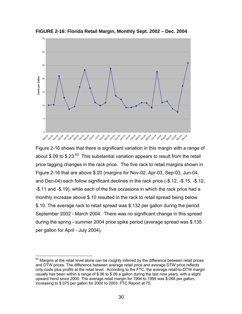
30

FIGURE 2-16: Florida Retail Margin, Monthly Sept. 2002 – Dec. 2004

0

5

10

15

20

25

30

35

Sep-02

Oct-02

Nov-02

Dec-02

Jan-0

3

Feb-03

Mar-03

Apr-03

May-03

Jun-0

3Ju

l-03

Aug-03

Sep-03

Oct-03

Nov-03

Dec-03

Jan-0

4

Feb-04

Mar-04

Apr-04

May-04

Jun-0

4Ju

l-04

Aug-04

Sep-04

Oct-04

Nov-04

Dec-04

Cen

ts p

er G

allo

n

Figure 2-16 shows that there is significant variation in this margin with a range of

about $.09 to $.23.63 This substantial variation appears to result from the retail

price lagging changes in the rack price. The five rack to retail margins shown in

Figure 2-16 that are above $.20 (margins for Nov-02, Apr-03, Sep-03, Jun-04,

and Dec-04) each follow significant declines in the rack price (-$.12, -$.15, -$.12,

-$.11 and -$.19), while each of the five occasions in which the rack price had a

monthly increase above $.10 resulted in the rack to retail spread being below

$.10. The average rack to retail spread was $.132 per gallon during the period

September 2002 - March 2004. There was no significant change in this spread

during the spring - summer 2004 price spike period (average spread was $.135

per gallon for April - July 2004).

63 Margins at the retail level alone can be roughly inferred by the difference between retail prices and DTW prices. The difference between average retail price and average DTW price reflects only costs plus profits at the retail level. According to the FTC, the average retail-to-DTW margin usually has been within a range of $.06 to $.08 a gallon during the last nine years, with a slight upward trend since 2000. The average retail margin for 1994 to 1999 was $.068 per gallon, increasing to $.075 per gallon for 2000 to 2003. FTC Report at 75.

31

Gasoline Taxes Gasoline sold to Florida consumers is taxed by the federal government,

the state government, and local governments. Federal gasoline taxes were

$.184 per gallon throughout the 2000 - 2004 period. Florida state tax on gasoline

increased from $.133 per gallon in 2000 to $.143 per gallon by December 200464.

In addition, local governments imposed taxes that range from $.055 to $.17 per

gallon.65 Such tax differences explain some of the differences in prices paid in

different parts of Florida. However, our interest is in changes in prices over time.

Since the local taxes changed very little over time, the variance across regions

will not be a significant factor in understanding gasoline prices over time.66 We

therefore utilize local taxes paid in Dade County to summarize trends in overall

tax rates in Florida.

Figure 2-17 summarizes the trends in the gasoline tax paid by Florida

consumers of gasoline. This includes the local gasoline taxes paid in Dade

County.

FIGURE 2-17: Florida Motor Fuel Tax Components, Annual 2000-2004 67

18.4 18.4 18.4 18.4 18.4 18.4

13.3 13.6 13.9 14.1 14.3

6.3

15.1 15.3 15.5 15.6 15.7

15.7

0

10

20

30

40

50

2000 2001 2002 2003 2004 Aug-04

Tota

l Tax

- Cen

ts p

er G

allo

n

Federal State Local

46.8 47.3 47.8 48.1 48.4

40.4

64 Source: http://www.myflorida.com/dor/taxes/fuel_tax.html. 65 Source: http://www.floridastategasprices.com/tax_info.aspx. 66 The largest change was in Suwannee county in 2002 where the local tax increased by $.06. 67 Sources: http://www.myflorida.com/dor/taxes/fuel_tax.html and http://sun6.dms.state.fl.us/dor/pdf/2000fuel.pdf.

32

August 2004 is separated out in the figure because in response to the high prices

of May and June, the Florida legislature passed a “gasoline tax relief” bill

temporarily lowering state taxes by $.08 per gallon for this month.68

The overall gasoline tax in Florida is among the highest in the nation. 69

This is shown in Table 2-1 below.

TABLE 2-1: Overall Gasoline Tax by State and Ranking, 2002

STATE Overall Gasoline Tax Ranking STATE Overall Gasoline Tax Ranking Hawaii 53.5 1 Arkansas 40.1 21 Nevada 51.7 2 Massachusetts 39.9 22 California 50.4 3 Kentucky 39.8 23 Wisconsin 49.5 4 Tennessee 39.8 23 Rhode Island 49.4 5 Iowa 39.5 24 New York 48.7 6 Alabama 39.4 25 Illinois 48.4 7 North Dakota 39.4 25 Connecticut 48.1 8 New Hampshire 39.0 26 Florida 48.0 9 Dist. of Columbia 38.4 27 Montana 46.2 10 Louisiana 38.4 27 Pennsylvania 45.1 11 Minnesota 38.4 27 Michigan 44.6 12 Texas 38.4 27 Nebraska 43.8 13 Vermont 38.4 27 West Virginia 43.8 13 Arizona 37.4 28 Idaho 43.4 14 Virginia 37.3 29 Utah 42.9 15 Mississippi 37.2 30 Kansas 42.4 16 Indiana 36.5 31 Oregon 42.4 16 New Mexico 36.4 32 South Dakota 42.4 16 Missouri 35.4 33 Maine 41.9 17 Oklahoma 35.4 33 Maryland 41.9 17 South Carolina 35.2 34 Delaware 41.4 18 New Jersey 32.9 35 Washington 41.4 18 Wyoming 32.4 36 North Carolina 40.8 19 Georgia 30.6 37 Colorado 40.4 20 Alaska 26.4 38 Ohio 40.4 20 US Average 42.0

68 Source: http://www.taxadmin.org/fta/meet/mf04_pres/mcelroy.pdf. 2004 data excludes August which is shown separately. 69 See, http://www.energy.ca.gov/gasoline/statistics/gas_taxes_by_state_2002.html.

33

In mid-2002, the total gasoline tax in Florida was about $.48 per gallon compared

to the U.S. average of about $.42 per gallon. Gasoline taxes in Florida are about

$.17 per gallon higher than in neighboring Georgia. Nonetheless, because our

interest is in understanding the reasons for the price spike of 2004, the relatively

constant (though high) Florida taxes play no role in such understanding.

High Crude Oil Costs and Refining Margins Account For the 2004 Price Spike Figures 2-18 and 2-19 summarize the components of the Florida gasoline

prices by industry stage. Figure 2-18 is for the period September 2002 through

2004 while Figure 2-19 is for the entire 2000-2004 period. We present these two

figures because we cannot separate the shipping and wholesaling margin from

the trucking and retailing margin before September of 2002.

FIGURE 2-18: Components of Florida Gasoline Price, by Relevant Period Sept. 2002 - Dec. 2004

61.9 66.974.2

81.696.2

14.920.3

29.2

40.624.5

6.8

6.3

5.9

6.5 8.7

13.6

13.8

10.1

13.5 14.2

47.8

48.1

48.4

48.4 46.8

0

20

40

60

80

100

120

140

160

180

200

220

2002 2003 Jan-Mar 2004 Apr-Jul 2004 Aug-Dec 2004

Cen

ts p

er G

allo

n

Crude Refining Margin Wholesale Margin Retail Margin Tax

145.0

155.5

167.7

190.6 190.4

34

FIGURE 2-19: Components of Florida Gasoline Price, by Relevant Period 2000-2004

60.374.2

81.696.2

18.8

29.2

40.624.5

18.4

16.0

20.0 22.9

47.5

48.4

48.4 46.8

0

20

40

60

80

100

120

140

160

180

200

220

2000-2003 Jan-Mar 2004 Apr-Jul 2004 Aug-Dec 2004

Cen

ts p

er G

allo

n

Crude Refining Margin Wholesale and Retail Margin Tax

145.0

167.7

190.6 190.4

Table 2-2 shows the changes in the gasoline price components from

period to period.

TABLE 2-2: Changes in Components of Florida Gasoline Price, by Relevant Period 2000-2004

Change over Period CRUDE REFINING MARGIN

WHOLESALE and RETAIL

MARGIN TAXES RETAIL

2000 to 2001 -11.81 2.33 1.41 0.50 -7.57

2001 to 2002 3.76 -5.85 -1.36 0.50 -2.95

2002 to 2003 10.23 5.12 2.82 0.30 18.47

2003 to Jan-Mar 2004 7.32 8.83 -4.17 0.30 12.28

Jan-Mar 2004 to Apr-Jul 2004 7.43 11.42 4.02 0.00 22.87

Apr-Jul 2004 to Aug-Dec 2004 14.55 -16.07 2.95 -1.60 -0.16

35

Crude oil prices decreased by about $.08 per gallon from 2000 to 2002 while the

average retail price decreased by nearly the same amount ($.105 per gallon).

During the 2002 – 2003 period, average annual crude oil prices increased by

$.102 per gallon, while average annual retail prices increased by about $.185.

Increased refining and wholesaling margins lie behind the greater increase in the

retail prices. In early 2004, crude oil prices increased again by more than $.07

per gallon and retail prices were up about $.12.70 By the spring–summer price

spike period, crude oil prices had continued to escalate, up about another $.075

per gallon from January to March. However, the retail price increase of almost

$.23 was more than triple the crude oil cost increase. This difference is

attributable to the increased refining margin (+$.114) and increased wholesale-

retail margin (+$.04). Crude oil prices then soared to record levels during the period August to

December 2004, averaging about $.22 per gallon more than in early 2004. The

average wholesale-retail margin also increased by almost $.03 per gallon later in

2004.71 Nonetheless, retail prices did not rise in late 2004, largely because of the

substantial decline in the average refining margin (-$.161 per gallon) back to

historic competitive levels.

Figure 2-20 shows the components of the Florida gasoline price by industry

stage by month for 2004.

70 Crude oil price in December 2003 was $.69 per gallon and retail price was $1.001 per gallon ($1.482 with tax). By April 2004, crude was $.7585 per gallon and retail was $1.319 per gallon ($1.809 with tax). Sources: EIA, Petroleum Marketing Monthly, Table 31, various months. 71 An increase of more than $.07 per gallon from early 2004.

36

FIGURE 2-20: Components of Florida Gasoline Price, Monthly 2004

73.6 71.5 77.4 75.885.0 81.8 83.8

94.6 92.1

108.697.9

87.6

24.8 31.231.6 39.0

48.4

35.439.5 23.1 31.9

26.1

25.8

15.75.1

5.96.7

6.1

3.5

8.87.8

9.14.7

8.2

10.3

11.39.39.8

11.110.9

9.222.6 11.1

11.5 8.8

7.617.3

25.9

48.448.4

48.4 48.448.4

40.4 48.4

48.4 48.4

48.4

48.448.4

0

20

40

60

80

100

120

140

160

180

200

Jan Feb Mar Apr May Jun Jul Aug Sep Oct Nov Dec

Cen

ts p

er G

allo

n

Crude Refining Margin Wholesale Margin Retail Margin Tax This figure again demonstrates the role of the increased refining-wholesale

margin in explaining the price spike of the spring-summer. From a typical or

average level in January of about $.30, the refining wholesale margin increased

to $.371 in February, then to $.383 in March, and then to $.451 in April, peaking

at over $.52 in May. While the refining-wholesale margin declined somewhat to

$.473 in July and to $.322 in August, these margins were at historically high

levels. However, it is important to note that margins then continued to decline to

normal levels by the end of the year.

This untangling of the Florida retail price indicates that during the spring-

summer gasoline price spike period, we do find significantly increased returns

being earned by the integrated refining and transportation segments of the

supply chain. Yet these high margins were reversed during the rest of the year,

with “average” or “typical” margins being restored by the end of 2004. In order to

better understand the cause of these changes in margins, we examine in the

next section the extent to which events in Florida may have been related to

37

factors specific to Florida (such as transportation bottlenecks, barge accidents or

shortages). We will then turn in Section 4 to an analysis of underlying supply and

demand conditions that impact the refining-wholesaling margins.

38

SECTION 3: WAS THE 2004 PRICE SPIKE SPECIFIC TO FLORIDA? COMPARISONS TO PRICES IN OTHER REGIONS

In the prior section of this report, we confirmed that high Florida gasoline

prices in 2004 were primarily attributable to high crude oil prices and high

refining-wholesale margins. Prices of both crude oil and Gulf Coast spot

gasoline are expected to be independent of events specific to Florida. However,

the rack price in Florida may incorporate factors specific to the transportation of

gasoline from the Gulf Coast to Florida, and both the rack price and the retail

price may result in part from competitive conditions specific to Florida. In this

section, therefore, we examine to what extent the high prices of 2004 are

“general” to the areas supplied by Gulf Coast refineries and/or to what extend the

high prices are related to factors specific to Florida.

Figure 3-1 shows monthly average retail prices by state for Florida, New

York, Illinois, Texas, California and for all of the United States.72

FIGURE 3-1: Average Retail Prices by State, Monthly 2000- 2004

40

60

80

100

120

140

160

180

200

Jan-0

0

Mar-00

May-00

Jul-0

0

Sep-00

Nov-00

Jan-0

1

Mar-01

May-01

Jul-0

1

Sep-01

Nov-01

Jan-0

2

Mar-02

May-02

Jul-0

2

Sep-02

Nov-02

Jan-0

3

Mar-03

May-03

Jul-0

3

Sep-03

Nov-03

Jan-0

4

Mar-04

May-04

Jul-0

4

Sep-04

Nov-04

Cen

ts p

er G

allo

n

Florida (PI) New York (PI) Illinois (PII) Texas (PIII) California (PV) US Average 72 Source: EIA, Petroleum Marketing Monthly, Table 31.

39

In this figure, the overall Florida prices appear to be consistently among the

lowest state prices. Figures 3-2 and 3-3 confirm this by examining the annual

average retail prices by state.

FIGURE 3-2: Average Retail Price by State, Annual 2000-2004

100.7

92.689.2

107.4

137.1

108.7

98.8

91.0

113.3

141.7

111.5108.3

96.5

113.1

140.3

98.8

91.086.4

103.3

130.3

114.9109.3

98.4

130.3

160.7

106.199.4

91.2

111.1

139.4

0

20

40

60

80

100

120

140

160

180

2000 2001 2002 2003 2004

Cen

ts P

er G

allo

n

Florida (PI) New York (PI) Illinois (PII) Texas (PIII) California (PV) US Average FIGURE 3-3: Average Retail Price by State for the Period 2000-2004

105.4110.7 113.9

101.9

122.7

109.5

0

20

40

60

80

100

120

140

Florida (PI) New York (PI) Illinois (PII) Texas (PIII) California (PV) US Average

Ave

rage

Ret

ail P

rice

- Cen

ts p

er G

allo

n

40

Table 3-1 gives the correlation coefficients among these states’ gasoline

prices.

TABLE 3-1: Correlation Coefficients Between Retail Prices by State, 2004 California Florida Illinois New York Texas US Average California n/a 0.9072 0.9042 0.8730 0.8782 0.9257 Florida 0.9072 n/a 0.9516 0.9902 0.9749 0.9782 Illinois 0.9042 0.9516 n/a 0.9421 0.9841 0.9924 New York 0.8730 0.9902 0.9421 n/a 0.9733 0.9697 Texas 0.8782 0.9749 0.9841 0.9733 n/a 0.9919 US Average 0.9257 0.9782 0.9924 0.9697 0.9919 n/a

This table shows a highly statistically significant correlation in prices between

states. The pattern of the correlations for the state prices is in line with economic

expectations. In particular, New York is supplied in substantial part by the same

refineries supplying Florida, and the Texas refineries are a major source of

Florida supply. As would be expected, the Florida prices are most like those in

Texas and New York and least like those in California.

Figure 3-4 shows average retail prices by PADD region and the average

for the entire United States.73

FIGURE 3-4: Average Retail Prices by Region, Monthly 2000-2004

40

60

80

100

120

140

160

180

200

Jan-

00

Mar-0

0

May-0

0

Jul-0

0

Sep-0

0

Nov-0

0

Jan-

01

Mar-0

1

May-0

1

Jul-0

1

Sep-0

1

Nov-0

1

Jan-

02

Mar-0

2

May-0

2

Jul-0

2

Sep-0

2

Nov-0

2

Jan-

03

Mar-0

3

May-0

3

Jul-0

3

Sep-0

3

Nov-0

3

Jan-

04

Mar-0

4

May-0

4

Jul-0

4

Sep-0

4

Nov-0

4

Cen

ts p

er G

allo

n

PADDI PADDII PADDIII PADDIV PADDV US Average 73 Source: EIA, Petroleum Marketing Monthly, Table 31.

41

Figure 3-5 shows the overall average prices by PADD for the entire period.

FIGURE 3-5: Average Retail Price by PADD for the Period 2000-2004

107.5109.5

104.6

112.1

121.6

109.5

95

100

105

110

115

120

125

PADDI PADDII PADDIII PADDIV PADDV US Average

Cen

ts p

er G

allo

n

PADD I, the petroleum region that includes Florida has relatively low prices,

about $.02 per gallon lower than the average for the U.S. PADD III, the PADD

which primarily supplies Florida, is the only region with consistently lower prices

of about $.03 per gallon.

Figure 3-6 compares the Florida average retail price to the overall PADD I

average. The Florida price is consistent with the prices in PADD I, with a

correlation coefficient of .9918. The Florida price is also generally below that of

the PADD I average; overall the Florida price is $.017 per gallon lower. The

correlation coefficient for PADD I and Florida retail prices for 2004, the year of

interest, is identical to the overall correlation of .9918.

42

FIGURE 3-6: Florida Retail Price Compared to PADD I Averages, Monthly 2000-2004

0

20

40

60

80

100

120

140

160

180

Jan-0

0

Mar-00

May-00

Jul-0

0

Sep-00

Nov-00

Jan-0

1

Mar-01

May-01

Jul-0

1

Sep-01

Nov-01

Jan-0

2

Mar-02

May-02

Jul-0

2

Sep-02

Nov-02

Jan-0

3

Mar-03

May-03

Jul-0

3

Sep-03

Nov-03

Jan-0

4

Mar-04

May-04

Jul-0

4

Sep-04

Nov-04

Cen

ts p

er G

allo

n

Florida PADD I The issue of significance in this section concerns not the absolute level of

Florida prices compared to other places but rather the extent to which the price

increases in Florida during the price spike period in 2004 were or were not

specific to Florida. Since the charts presented in this section indicate relative

independence in the prices in PADD V, we focus hereafter on cities and states in

PADDs I-IV. Figure 3-7 shows the average prices, by year, with 2004 broken

into the sub-periods of January through March, April through July, and August

through December, for Miami, Houston, Atlanta, Chicago, and New York City.

43

FIGURE 3-7: Average Retail Prices by City, by Relevant Period 2000-2004

109.3106.2

121.1125.8

108.9

100.5 100.7

118.2

128.2

99.394.5

86.0

98.8

112.5

86.6

115.7 113.5

127.5132.8

107.2

122.8118.9

133.3139.5

119.2

149.2145.0

156.8

167.5

142.3

152.0

134.0

157.9

169.1

139.6

0

20

40

60

80

100

120

140

160

180

Atlanta (PI) Miami (PI) New York (PI) Chicago (PII) Houston (PIII)

Cen

ts p

er G

allo

n

2000 2001 2002 2003 Jan-Mar 2004 Apr-Jul 2004 Aug-Dec 2004

The figure appears to indicate substantial price increases in each of the cities

during the April-July 2004 spike period. This is confirmed in Table 3-2 which

shows the changes in prices between each of these periods.

TABLE 3-2: Change in Retail Prices within Cities, by Relevant Period 2000-2004

Change In Retail Price

Change Over Period Atlanta (PI)

Miami (PI)

New York (PI)

Chicago (PII)

Houston (PIII)

2000 to 2001 -8.8 -5.5 -2.9 2.4 -9.7 2001 to 2002 -6.0 -14.7 -19.5 -15.7 -12.7 2002 to 2003 21.3 27.5 28.7 20.3 20.7

2003 to Jan-Mar 2004 7.1 5.4 5.8 6.7 12.0 Jan-Mar 2004 to Apr-Jul 2004 26.4 26.1 23.4 27.9 23.1 Apr-Jul 2004 to Aug-Dec 2004 2.7 -11.0 1.1 1.6 -2.6

Overall, the prices in other cities increased in similar fashion to those in Miami.

Figure 3-8 shows the average prices for the states of Florida, Texas,

Illinois, and New York broken into the same periods as in Figure 3-7.

44

FIGURE 3-8: Average Retail Prices by State, by Relevant Period 2000-2004

100.7

108.7111.5

98.8

92.6

98.8

108.3

91.089.2 91.096.5

86.4

107.4113.3 113.1

103.3

119.3123.5 123.1

112.3

142.2147.0 146.8

135.3

143.6148.4

145.5

137.0

0

20

40

60

80

100

120

140

160

Florida (PI) New York (PI) Illinois (PII) Texas (PIII)

Cen

ts p

er G

allo

n

2000 2001 2002 2003 Jan-Mar 2004 Apr-Jul 2004 Aug-Dec 2004

Again, as shown in Table 3-3, the price increases of 2004 were general to these

states rather than specific to Florida.

TABLE 3-3: Change in Retail Prices within States, by Relevant Period 2000-2004

Change in Retail Price

Change Over Period Florida New York Illinois Texas 2000 to 2001 -8.1 -9.9 -3.2 -7.8 2001 to 2002 -3.5 -7.7 -11.8 -4.6 2002 to 2003 18.2 22.3 16.7 16.9

2003 to Jan-Mar 2004 12.0 10.3 9.9 9.0 Jan-Mar 2004 to Apr-Jul 2004 22.9 23.4 23.7 22.9 Apr-Jul 2004 to Aug-Dec 2004 1.4 1.4 -1.3 1.7

During the April - July 2004 price spike period, the average retail price in each of

the comparison states and Florida increased by about $.23 per gallon compared

to the pre-spike period. After the price spike period, New York and Texas saw a

similar small price increase like the one experienced in Florida. The price in

Illinois did fall in the latter part of 2004. However, Illinois had the largest increase

45

during the price spike period and it is relatively more isolated from the Gulf Coast

supply effects.

These price comparisons clearly demonstrate that the spring–summer

2004 price spike and the high prices of 2004 are general industry phenomena

and not the result of a problem specific to Florida. As a consequence of this

conclusion, in Section 4 we seek economic explanations for the 2004 increases

in Florida gasoline prices that relate to general economic factors impacting the

spot price of gasoline and the rack price of gasoline. The international factors

impacting the price of crude oil are beyond the scope of this Report.74

Specifically, we will analyze supply and demand factors important in the supply of

gasoline from Gulf Coast refineries in an attempt to understand better the

variations in the refining-wholesale margins that occurred during the price spike

period.

74 International events underlying the precipitous increase in crude oil prices are discussed in the FTC Report, Chapter 5.

46

SECTION 4: SUPPLY AND DEMAND ANALYSIS OF FLORIDA GASOLINE PRICES

We determined in Section 2 that the major cost component of gasoline in

Florida is the price of crude oil. The price of crude oil is determined in an

international market subject to the supply restrictions of OPEC and to

international events that disrupt the flow of crude oil from the Middle East. The

integrated petroleum companies that provide the bulk of gasoline to Florida have

a substantial ownership interest in crude oil. Therefore, the fortunes of the

integrated petroleum companies are closely related to the price of crude oil. For

the purposes of our analysis, we shall take the price of crude oil as given. Our

goal will be to examine the other components of the Florida gasoline price to see

whether competitive supply and demand conditions explain the movements in

these price components.

Under reasonable competition, gasoline prices will generally keep pace

with underlying costs of “production” at each stage of supply, including a normal

level of profit. However, in the short term, gasoline prices can rise above the

long run competitive level as the balance between supply and demand shifts.

From the analysis in Sections 1 and 2 of this Report, we have concluded that the

marketing and retailing of gasoline is relatively competitive with little ability to

significantly impact the market price of gasoline. This conclusion follows from

both the structure of this sector (many terminals, many jobbers, and many

gasoline supply outlets) and from the relatively constant margins earned in this

sector regardless of the overall price of gasoline. Hence, the retail price to

consumers will essentially be the price at the rack plus the competitive costs of

marketing and retailing. In this section, we therefore focus mainly on the extent

to which refining, shipping, and distribution margins are at reasonably

competitive levels both during and after the price spike period. We begin by

briefly examining the overall profitability of the integrated petroleum refiners. We

then turn to an analysis of the relevant supply and demand variables that

determine the price of gasoline in Florida. Our goal is to ascertain the extent to

47

which such supply and demand variables “explain” the high prices of gasoline in

Florida (and other areas) in 2004.

The Earnings of Integrated Petroleum Refiners

Overall Earnings Are Driven By Crude Oil Revenues

The Energy Information Administration collects detailed financial data from

a set of petroleum companies that comprise most of the refining capacity in the

U.S.75 This data allows for the calculation of the return on equity for petroleum

companies. This return on equity provides an index of the overall industry

profitability. The EIA data incorporate profits earned at all vertical stages of

production including of crude oil, refining, transportation, distribution, and

marketing.

The overall rate of return on stockholders' equity for EIA petroleum

companies between 1977 and 2001 was somewhat in excess of 12 percent. In

the more recent period, 2000-2003, the return on equity increased to an average

of 14.5 percent. In 2002, the return on equity was only 9.4 percent as a result of

generally weaker crude oil prices, an economic downturn, and the aftermath of

the September 11 attacks. However, the years 2000 and 2003 show very high

returns on equity of 19.6 percent and 18.1 percent respectively.76 As a general

conclusion, the overall petroleum companies’ return on equity is in the general

range of that achieved by other large companies. According to EIA data, the

reporting petroleum companies' rate of return on equity was 12.6 percent while

the average return for Standard & Poor’s industrials was 13.2 percent.

The return on equity for the petroleum companies is mainly influenced by

changes in the price of crude oil and not by what happens in the domestic

markets for the refining of petroleum and sale of refined products. Thus, the

petroleum companies fared poorly in the late 1980s and early 1990s when crude

oil prices were relatively low. However, in times of high crude oil prices, these 75 See, EIA, Companies Reporting to the Financial Reporting System, 1974-2002, available at http://www.eia.doe.gov/aer/txt/ptb0312.html. These companies represented about 84% of refining capacity in 2003. EIA, Performance Profiles of Major Energy Producers 2003, Table B1. 76 Source: EIA, Performance Profiles of Major Energy Producers 2003, Figure 2 Data.

48

firms did well. In particular, the 2000s have been good years, with 2004 being a

particularly strong year. In 2004, the single most profitable company in the

Fortune 500 was ExxonMobil with ChevronTexaco ranking fifth.77 The petroleum

refining industry had the second highest growth in profits of the 47 industries with

reported data. The petroleum refining industry offered the fourth highest overall

return to stockholders in 2004 of any reported industry.78

Earnings from Refining

From the analysis of Section 2 above, the average “integrated margin”

(Florida rack price minus Gulf Coast crude cost) earned by Gulf Coast refineries

from refining and transportation for the period 2000 through 2003 was $.189 per

gallon. This margin did increase substantially over the period February through

July 2004 to $.395 per gallon with a peak in May of $.485. These high margins

were followed, however, by a decline in margins back to historical and

competitive levels. These margins, as defined and calculated in Section 2, take

into account only the price of gasoline. These margins may not, therefore,

represent an overall accurate picture of refining profitability.

The EIA data provides refining margin information based on the value of

the complete slate of products produced by a typical refinery. The EIA gross and

net refining margins are presented in Figure 4-1.79

77 http://www.fortune.com/fortune/subs/fortune500/topperformers/0,23620,,00.html 78 “Petroleum Refining” as defined by Fortune includes the large integrated companies such as ExxonMobil, ChevronTexaco, ConocoPhillips and Marathon. In the Fortune Global 500, which includes BP and Shell, in addition to the domestic companies, the petroleum refining industry had the 4th highest (of 36) return on assets for 2004. 79 Source: EIA, Performance Profiles of Major Energy Producers 2003, Figure 5. "Gross margin" is defined as total product revenue less crude oil input into refineries. "Operating costs" consist of refinery energy costs, other refinery expenses, and marketing expenses. "Net margins" are the difference between gross margin and operating costs. These data are not strictly indicative of refinery margins, as they do not distinguish between the refinery and marketing operations of the FRS companies.

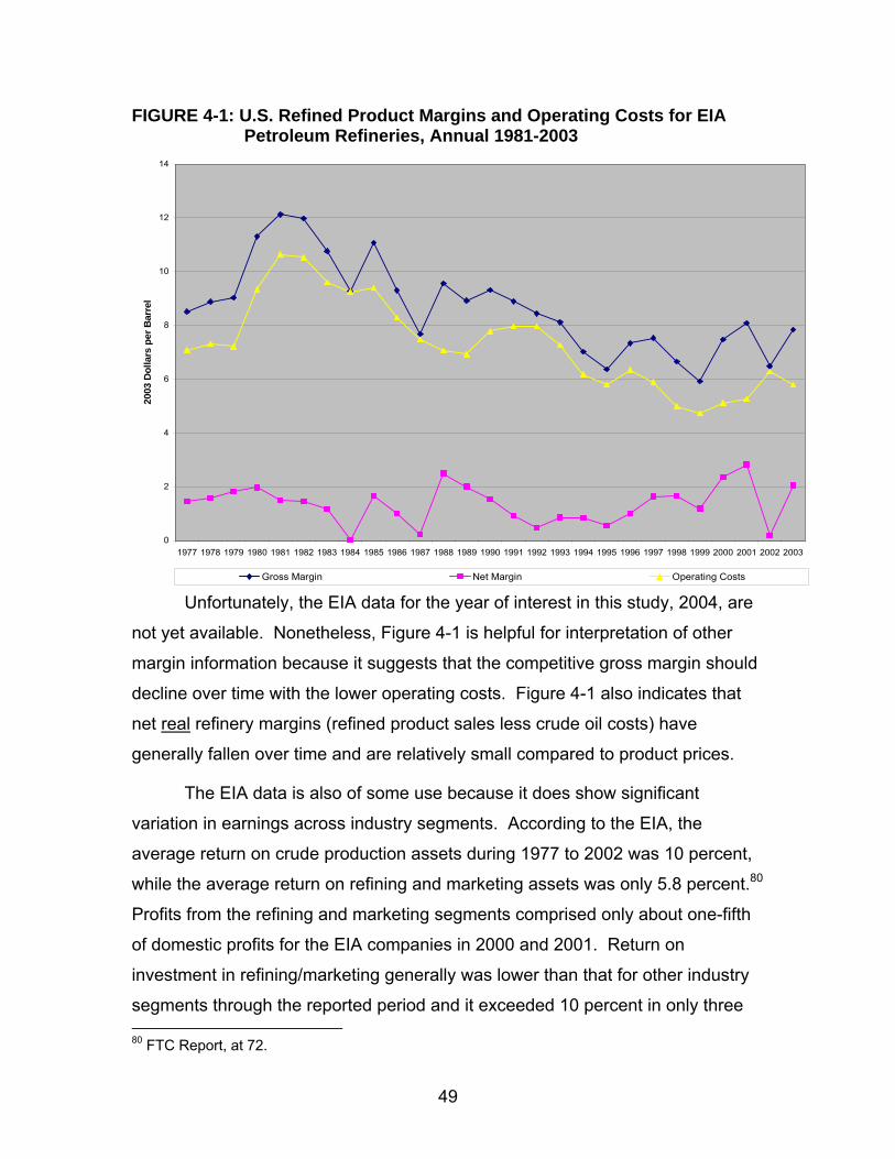
49

FIGURE 4-1: U.S. Refined Product Margins and Operating Costs for EIA Petroleum Refineries, Annual 1981-2003

0

2

4

6

8

10

12

14

1977 1978 1979 1980 1981 1982 1983 1984 1985 1986 1987 1988 1989 1990 1991 1992 1993 1994 1995 1996 1997 1998 1999 2000 2001 2002 2003

2003

Dol

lars

per

Bar

rel

Gross Margin Net Margin Operating Costs Unfortunately, the EIA data for the year of interest in this study, 2004, are

not yet available. Nonetheless, Figure 4-1 is helpful for interpretation of other

margin information because it suggests that the competitive gross margin should

decline over time with the lower operating costs. Figure 4-1 also indicates that

net real refinery margins (refined product sales less crude oil costs) have

generally fallen over time and are relatively small compared to product prices.

The EIA data is also of some use because it does show significant

variation in earnings across industry segments. According to the EIA, the

average return on crude production assets during 1977 to 2002 was 10 percent,

while the average return on refining and marketing assets was only 5.8 percent.80

Profits from the refining and marketing segments comprised only about one-fifth

of domestic profits for the EIA companies in 2000 and 2001. Return on

investment in refining/marketing generally was lower than that for other industry

segments through the reported period and it exceeded 10 percent in only three 80 FTC Report, at 72.

50

years (1988, 1989, and 2001). Of particular note, for the last year with available

data, 2002, the EIA petroleum companies suffered a record $2.2 billion loss on

domestic refining and marketing operations.81 Given this, considered over the

scope of a refinery’s life, any increase in refining margins in the spring and

summer of 2004 certainly cannot be interpreted as indicating excessive long run

economic profit.

We can get some more detailed information on overall refinery margins by

use of the "crack spreads" -- a common measure used to indicate the profitability

of refineries. The "crack spread" is typically based on a hypothetical refinery

producing two gallons of gasoline and one gallon of diesel for every three gallons

of crude oil. Figure 4-2 shows the monthly crack spreads (in current dollars) for

the period 2000 through 2004 for New York harbor spot prices. 82

FIGURE 4-2: Refinery Crack Spreads on NY Spot Prices, Monthly 2000-2004

0

5

10

15

20

25

30

35

Jan-0

0

Mar-00

May-00

Jul-0

0

Sep-00

Nov-00

Jan-0

1

Mar-01

May-01

Jul-0

1

Sep-01

Nov-01

Jan-0

2

Mar-02

May-02

Jul-0

2

Sep-02

Nov-02

Jan-0

3

Mar-03

May-03

Jul-0

3

Sep-03

Nov-03

Jan-0

4

Mar-04

May-04

Jul-0

4

Sep-04

Nov-04

Cen

ts p

er G

allo

n

81 FTC Report, at 72. 82 Sources: http://www.eia.doe.gov/emeu/international/crude2.html; http://www.eia.doe.gov/neic/historic/hpetroleum2.htm - links Gasoline Spot and Diesel Spot.

51

The real crack spread has averaged about $.095 per gallon since 1986.

The spread reached an historical high of over $.20 per gallon in spring 2001, but

then fell to more typical levels in 2002. Figure 4-3 shows the same general

pattern of increased margins during the spring-summer price spike period for

New York Harbor diesel and gasoline spot prices. The crack spread increases

somewhat during the 2004 price spike period, up $.09 from the average January

2000 to March 2004 levels. This is certainly expected since this margin is

dominated by gasoline prices. However, this measure of the refining margin

does not show as great an impact as the margin based solely on gasoline prices.

This is because diesel prices did not exhibit the same price spike as did gasoline

prices.

Figure 4-3 graphs the New York harbor diesel and gasoline spot prices.

FIGURE 4-3: NY Spot Prices of Gasoline and Diesel, Monthly 2000-2004

0

20

40

60

80

100

120

140

160

180

Jan-0

0

Mar-00

May-00

Jul-0

0

Sep-00

Nov-00

Jan-0

1

Mar-01

May-01

Jul-0

1

Sep-01

Nov-01

Jan-0

2

Mar-02

May-02

Jul-0

2

Sep-02

Nov-02

Jan-0

3

Mar-03

May-03

Jul-0

3

Sep-03

Nov-03

Jan-0

4

Mar-04

May-04

Jul-0

4

Sep-04

Nov-04

Cen

ts p

er G

allo

n

Gasoline Diesel

If the price spike were “explained” solely by crude oil price increases, we would

expect the prices of all refined products to show similar increases. Figure 4-3

52

indicates that this is not true for the second most significant refined product -

diesel fuel. NYMEX crude oil prices were up about $.13 per gallon during the

spike period. Diesel prices increased only about $.09 per gallon, while gasoline

prices rose about $.205 per gallon.83

Supply and Demand Factors Impacting the Refining-Shipping Margin Gas Demand

We now turn to examination of the extent to which supply and demand of

gasoline explains the high gasoline prices paid by Florida consumers in 2004.

Figure 4-4 shows U.S. gasoline consumption from 1970 through 2003 measured

in BTUs.84 Figure 4-5 shows U.S. gasoline consumption in gallons 1995-2004.85

Figure 4-6 shows gasoline consumption for Florida in average gallons per day.86

FIGURE 4-4: US Gasoline Consumption, Annual 1970-2003

0

5,000,000

10,000,000

15,000,000

20,000,000

25,000,000

30,000,000

1970

1971

1972

1973

1974

1975

1976

1977

1978

1979

1980

1981

1982

1983

1984

1985

1986

1987

1988

1989

1990

1991

1992

1993

1994

1995

1996

1997

1998

1999

2000

2001

2002

2003

Mill

ion

BTU

83 The diesel prices did increase substantially more rapidly than either crude oil or gasoline prices after the gasoline price spike. Crude oil was up $.19 per gallon August - December as compared to April - July. Over the same period, diesel prices rose $.315, while gasoline prices rose only $.025. 84 EIA, Annual Energy Review, Energy Consumption by Sector, Table 2.1 85 Source: EIA, Petroleum Supply Annual Volume 1, Table 2, various years. 86 Source: EIA, Petroleum Marketing Annual, Table 48, various years.

53

FIGURE 4-5: US Gasoline Consumption, Annual 1995-2004

105,000,000

110,000,000

115,000,000

120,000,000

125,000,000

130,000,000

135,000,000

140,000,000

145,000,000

1995 1996 1997 1998 1999 2000 2001 2002 2003 2004

1000

Gal

lons

FIGURE 4-6: Florida Gasoline Consumption, Annual 1995-2004

15,000

16,000

17,000

18,000

19,000

20,000

21,000

22,000

23,000

24,000

25,000

1995 1996 1997 1998 1999 2000 2001 2002 2003 2004

1000

Gal

lons

per

Day

54

Figure 4-4 reflects a decline in gasoline consumption during the late 1970s and

early 1980s, largely in response to high prices during that time. Domestic

consumption has, however, steadily increased since the mid-1980s. Between

1995 and 2004, U.S. consumption of gasoline increased on average by 1.73

percent per year, from 119.4 billion gallons to 139.3 billion gallons, for a total

increase of 16.7 percent. Florida consumption has been increasing even more

rapidly, increasing about 2.7 percent per year since 1995.

Gasoline consumption is influenced by a number of demand factors

including the population, income, and the characteristics of vehicles. These

“demand” variables are available only on an annual basis and are not yet

available for 2004. Because each of the relevant demand variables are expected

to change only slowly and to change regularly, we include a “trend” variable in

the subsequent analysis to account for the changes in any important demand

factors.

Gasoline Supply

On the supply side, we need to take account of the ability of refineries to

supply gasoline to Florida and how that supply ability may have changed over

time. No successful new petroleum refinery has been built in the United States in

the last thirty years. This is due to the substantial barriers to entry into refining in

the United States. These barriers continue to grow: refineries have become

highly capital intensive and, more importantly, environmental restrictions continue

to become more onerous. Most industry experts do not expect new entry into

U.S. refining in the foreseeable future.87 Some additions to the capacity of

existing refineries are likely, but any future gasoline supply increases will mainly

have to be from imports.

In addition to practical limits to expansions of U.S. gasoline refining

capacity, regulations governing certain environmental characteristics of gasoline

reduce substitutability among refiners' differing gasoline products, which can

mean less ability to moderate price spikes through increased supply from other 87 See, e.g., EIA, Annual Energy Outlook 2003, at 83.

55

refineries. For example, Gulf Coast refineries make substantial amounts of

relatively expensive reformulated gasoline that is not needed in Florida. Only if

there is a very substantial increase in the relative price of gasoline in Florida will

reformulated gasoline be used to moderate that increase.

Figure 4-7 shows the total capacity of U.S. refineries from 1996 through

2003.88

FIGURE 4-7: Total U.S. Refinery Capacity, Annual 1996-2003

14500

15000

15500

16000

16500

17000

17500

1996 1998 1999 2000 2001 2002 2003

1000

Bar

rels

per

Cal

enda

r Day

Since 1998, U.S. refinery capacity increased by 0.7 percent per year. During the

same period, consumption grew by 1.6 percent per year. These facts alone

suggest increasing pressure on refined product prices.

United States refinery production has been by far the primary source for

domestic gasoline products, meeting on average over 94 percent of domestic

demand annually. However, as shown in Figure 4-8, refined gasoline product

88 Source: EIA, Petroleum Supply Annual Volume 1, Table 36, various years. This figure is not available for 1997.

56

imports are playing a somewhat more important role in balancing demand and

domestic supply.89

FIGURE 4-8: Gasoline Imports as a Percent of U.S. Consumption, Annual 1995-2004

3.4%

4.3%3.9% 3.8%

4.5%

5.0%5.3%

5.6% 5.8%

5.3%

0%

1%

2%

3%

4%

5%

6%

1995 1996 1997 1998 1999 2000 2001 2002 2003 2004

While the number of refineries in the U.S. has been decreasing, the

capabilities of the refineries that continue to operate have increased and more

than offset the capacity lost through shutdowns. The average distillation capacity

of operable U.S. refineries increased from about 72 million barrels per day in

1986 to 113 million barrels per day in 2004. Some of this increase is the result of

the closure of smaller, inefficient refineries but much of the increased capacity

per refinery resulted from investments in complex downstream processes that

increase the yield of light products including gasoline. The increasing

sophistication of refineries is indicated by the increased reliance on vacuum

distillation (distillation under reduced pressure), thermal cracking (which converts 89 Sources: EIA, Petroleum Supply Annual, Volume 1, Table 20, various years; EIA, Petroleum Supply Monthly, February 2005, Table 34.

57

heavier, larger molecules into lighter, smaller ones to boost the yields of light

product such as gasoline), catalytic cracking and catalytic hydrocracking

(advanced molecule cracking techniques), and catalytic reforming (use of a

catalyst to rearrange oil molecules to increase octane values).

The trend towards larger refineries90 and mergers among refining

companies has certainly increased the overall concentration of petroleum

refining, though, as discussed in Section 1, the industry is at the lowest threshold

of a “moderately” concentrated industry. PADD III refinery capacity concentration

in 2003 implied an HHI of 1018 (an increase of 419 since 1985). This increase is

mainly attributable to mergers of Exxon and Mobil; Chevron and Texaco; BP and

Amoco; Valero and UDS; and Phillips, Tosco and Conoco. The closure of a

number of small refineries also increased refining concentration.

The output from domestic refineries depends not only on their capacity but

also on the utilization of that capacity. Figure 4-9 shows the average annual

refining utilization for PADD III refineries for the period 1995 through 2004.91

Annual refinery utilization rates have averaged 94.4 percent for that period with a

1998 peak level of 96.7 percent. The utilization rate in 2004 was slightly below

average at 94.3 percent.

90 According to the FTC Report, Table 7-2, average refinery size increased by 53 million barrels per day in PADD I and by 61 million barrels per day in PADD II between 1986 and 2004. The corresponding increases in PADDs III, IV, and V were 49, 10, and 28 million barrels per day, respectively. 91 Sources: EIA, Petroleum Supply Annual, Volume 1, Table 16, various years; EIA, Petroleum Supply Monthly, Tables 28, various months.

58

FIGURE 4-9: PADD III Refining Capacity Utilization, Annual 1995-2004

75%

80%

85%

90%

95%

100%

1995 1996 1997 1998 1999 2000 2001 2002 2003 2004

FIGURE 4-10: PADD III Refining Capacity Utilization, Monthly 2000-2004

80%

82%

84%

86%

88%

90%

92%

94%

96%

98%

100%

Jan-0

0

Mar-00

May-00

Jul-0

0

Sep-00

Nov-00

Jan-0

1

Mar-01

May-01

Jul-0

1

Sep-01

Nov-01

Jan-0

2

Mar-02

May-02

Jul-0

2

Sep-02

Nov-02

Jan-0

3

Mar-03

May-03

Jul-0

3

Sep-03

Nov-03

Jan-0

4

Mar-04

May-04

Jul-0

4

Sep-04

Nov-04

59

Figure 4-10 shows the monthly refining capacity utilization for the period

2000-2004. The first relevant and striking feature of this figure is the unusually

low utilization in early 2004. These low utilizations presumably result from the

requirements to switch to low sulfur gasoline, to switch out of Methyl Tertiary

Butyl Ether (MTBE), and to the seasonal refinery turnaround in the winter.

However, these low utilization rates were shortly followed by unprecedented high

capacity utilizations shortly after the spring-summer 2004 price spike. By May

2004, PADD III refineries were producing refined product equal to 98.9% of their

rated capacity. In May, the output of domestic refineries was higher than ever

before. In June, the refining utilization was at a non-sustainable level of 99.4

percent. Over the four month period May-August 2004, refinery utilization

averaged 98.9 percent. In no other single month was such a high rate of

utilization reached. These very high utilization rates imply essentially no

remaining flexibility in domestic supply to counter any other supply or demand

factors leading to price increases.

Gasoline Inventories

Given the relatively high domestic utilization rates, the major short run

(prior to the movement of imported refined product) industry response to high

gasoline prices will be to increase supply out of inventory. Because consumption

requirements at any point in time are uncertain, and because of the lumpiness of

product supply (e.g., barge shipments), inventories are the mechanism used to

balance gasoline supply and gasoline consumption within a consumption area.

Therefore, the level of inventory in a region will provide a measure of the ability of

“supply” to quickly respond to any factors that otherwise would cause large price

spikes (e.g., refinery disruptions and unexpectedly large demand). Gasoline

inventories and changes in inventories, therefore, both measure and preview

market “tightness” (higher expected prices) or market “slack” (lower expected

prices). Rising and high inventories indicate available supply exceeding

consumption while falling and low inventories indicate consumption exceeding

60

available supply.92 Figure 4-11 shows the monthly inventories of gasoline for the

U.S., 2000 - 2004.93

FIGURE 4-11: U.S. Gasoline Inventories, Monthly 2000-2004

120,000

130,000

140,000

150,000

160,000

170,000

180,000

Jan-

00

Mar-0

0

May-0

0

Jul-0

0

Sep-0

0

Nov-0

0

Jan-

01

Mar-0

1

May-0

1

Jul-0

1

Sep-0

1

Nov-0

1

Jan-

02

Mar-0

2

May-0

2

Jul-0

2

Sep-0

2

Nov-0

2

Jan-

03

Mar-0

3

May-0

3

Jul-0

3

Sep-0

3

Nov-0

3

Jan-

04

Mar-0

4

May-0

4

Jul-0

4

Sep-0

4

Nov-0

4

1000

Bar

rels

Figure 4-12 shows the monthly inventories of gasoline for PADD I, 2000 - 2004.

FIGURE 4-12: PADD I Gasoline Inventories, Monthly 2000-200494

30,000

35,000

40,000

45,000

50,000

55,000

60,000

Jan-

00

Mar-0

0

May-0

0

Jul-0

0

Sep-0

0

Nov-00

Jan-

01

Mar-0

1

May-01

Jul-0

1

Sep-0

1

Nov-0

1

Jan-

02

Mar-02

May-0

2

Jul-0

2

Sep-0

2

Nov-0

2

Jan-

03

Mar-0

3

May-0

3

Jul-0

3

Sep-0

3

Nov-0

3

Jan-

04

Mar-0

4

May-0

4

Jul-0

4

Sep-0

4

Nov-0

4

1000

Bar

rels

92 Gasoline inventories will have a predictable seasonality, building in anticipation of the peak summer demand and falling during the peak driving period. 93 Sources: EIA, Petroleum Supply Annual, Volume 2, Table 2, various years; EIA, Petroleum Supply Monthly, Tables 2, various months. 94 Sources: EIA, Petroleum Supply Annual, Volume 2, Table 4, various years; EIA, Petroleum Supply Monthly, Table 6, various months.

61

Both Figures 4-11 and 4-12 show record low inventories in the period preceding

the price spikes of 2004. The average inventory in PADD I from November 2003

to February 2004 was 9 percent below the average for the same months for the

three prior years. The inventory in February for the U.S. and for PADD I was the

smallest of any month in 2000-2004 even though consumption had steadily

increased throughout this period.95

Figure 4-13 reinforces the very tight supply situation going into the spring

of 2004. This figure compares the PADD I inventory to consumption measured

by the days of supply for the coming month that the inventory could supply. The

figure shows that the inventories for the three months preceding the price spike

of the spring-summer 2004 were at record lows. As noted earlier, this was due to

both a decline in inventories and a spike in consumption. More gasoline was

consumed in March 2004 than ever recorded before in Florida (and PADD I).

The average days of supply inventory for January through March 2004 was 21

percent below that of the prior four years. In the concluding section, we discuss

in further detail the significance of the low inventories to the high gasoline prices

in Florida in early 2004.

95 Given the interdependence in gasoline supply throughout the PADD I region, the overall inventories in the region, rather than the inventory level in any particular state, is the most relevant supply variable.

62

FIGURE 4-13: Days of Supply PADD I Gasoline Inventory, Monthly 2000-200496

0

5

10

15

20

25

Jan-0

0

Mar-00

May-00

Jul-0

0

Sep-00

Nov-00

Jan-0

1

Mar-01

May-01

Jul-0

1

Sep-01

Nov-01

Jan-0

2

Mar-02

May-02

Jul-0

2

Sep-02

Nov-02

Jan-0

3

Mar-03

May-03

Jul-0

3

Sep-03

Nov-03

Jan-0

4

Mar-04

May-04

Jul-0

4

Sep-04

Nov-04

Day

s

Regression Analysis of the Refining-Wholesaling Margin and Florida Gas Prices The various supply and demand variables we have discussed imply a

market that was ripe for a price spike. Crude oil prices were rising; consumption

increases had been exceeding industry capacity increases; and, heading into the

peak spring-summer driving seasons, inventories were at record low levels. The

goal of Section 4 is to determine the extent to which the low inventories and other

standard supply and demand variables explain the spring-summer 2004 price

spike.

Regression analysis is a widely accepted statistical tool frequently used by

economists in research. “Multiple regression analysis is a statistical tool for

understanding the relationship between two or more variables.”97 Multiple

96 Sources: EIA, Petroleum Supply Annual, Volume 2, Table 5, various years; EIA, Petroleum Supply Monthly, Tables 8, various months. 97 Daniel Rubinfeld, “Reference Guide to Multiple Regression,” in Reference Manual on Scientific Evidence, Federal Judicial Center, 1994, at 419. Multiple regression simply refers to multiple

63

regression simply refers to the inclusion of multiple independent or explanatory

variables in the analysis. The “dependent” variables we seek to explain in the

regression analysis are: 1) the price of gasoline to Florida consumers and 2) the

refining margins earned by PADD III refineries.

On the demand side, the first explanatory variable is simply a trend

variable to account for the growth in demand from growing population, increasing

income, and reduced vehicle mileage caused by the SUV boom.

We also include a “seasonal” variable to measure changes in demand

from exogenous changes in driving. Winter is defined as December, January,

and February. Spring and summer are equivalently defined. Fall is the excluded

comparison season.

The supply variables include the inventory level as defined by the monthly

days of supply inventory. We lag this variable in the regression analysis; that is,

we use the month-end inventory measure of the preceding month to explain the

prices and refining margins in the current month.

In our analysis of the Florida gasoline price, we also include the inflation -

adjusted price of crude oil to the Gulf Coast refineries in the prior month. In our

refining margin analysis, the cost of crude oil has been netted out. However, we

do include a variable measuring the change in the cost of crude in order to

measure any lags in the ability of refiners to pass on this cost.

We also include a variable for possible impact of any supply disruptions

due to a barge collision on the Mississippi River that occurred in late February

2004 and a power blackout in late August 2003. We allow for any supply impact

of this via a 0-1 dummy variable with a value of 1 for the months of February and

March 2004 and August 2003.98

variables being used to explain another variable. For example, a multiple regression analysis could be conducted to “explain” people’s weight in which multiple “explanatory” variables might include height, waist size, and wrist size. 98 On February 27, 2004, two vessels collided near the mouth of the Mississippi River, closing the river for four days. On August 24, 2003 there was a power blackout in the North-East that led to wide-spread disruptions.

64

To control for inflation, we measure the dependent variables (the prices

paid for gasoline in Florida and, alternatively, the refining-wholesaling margins) in

real terms by deflating the nominal monthly prices by the Producer Price Index.

Finally, we include a 0-1 dummy variable for the price spike period of April

through July 2004. A positive and statistically significant coefficient on this

variable will indicate that the increase in the Florida gasoline price or in the

PADD III refining margin is not fully explained by the historical relationships

between these variables and the included explanatory variables.

The basic regression equation is a reduced form specification as

summarized in equations 4.1 and 4.2:

4.1. Pi=c+α1*COi+α2*INVi+α3*Ti+α4*BIi+αj*SEASi+αk*SPIKEi+εi

4.2. Ri= c+α1*∆COi+α2*INVi+α3*Ti+α4*BIi+αj*SEASi+αk*SPIKEi+εi

where: Pi is the Florida gasoline price in month i, Ri is the PADD III refining margin in month i, c is the regression constant, COi is the real price of crude oil in month i-1, ∆COi is the change real price of crude oil in month i-1, INV represents the days supply inventory variables for month i-1, T i is the trend variable, BIi is the barge incident dummy variable, SEAS represents the seasonal dummy variables, and εi is the error term.

Table 4-1 summarizes the results of this regression specification.

65

TABLE 4-1: Regression Results Summary Independent Variable: RETAIL PRICE R-Square 0.86352

Variable Co-

Efficient T-Value Intercept 57.95 2.57 Crude Oil Price 1.13 11.09 PADD I Days of Supply -1.90 -1.60 Trending Dummy -0.01 -0.09 Barge Issue Dummy 2.27 0.49 Price Spike Period Dummy 8.50 1.80 Winter Season Dummy 1.95 0.66 Spring Season Dummy 10.71 3.92 Summer Season Dummy 6.93 2.41

Independent Variable: REFINING MARGIN R-Square 0.55894

Variable Co-

Efficient T-Value Intercept 48.97 3.03 Crude Oil Price Change 0.23 1.64 PADD I Days of Supply -1.85 -1.87 Trending Dummy -0.08 -1.13 Barge Issue Dummy 7.23 1.74 Price Spike Period Dummy 13.46 3.18 Winter Season Dummy 2.31 0.87 Spring Season Dummy 7.20 2.97 Summer Season Dummy 2.64 1.01

The independent variables in the retail price regression explain 86 percent of the

variation in the price. The coefficients on the crude oil price, the inventory

measure, and the barge incident are of the expected signs, with the estimated

coefficients statistically significant for the crude oil variable and the inventory

variable. The independent variables in the refining margin regression explain 56

percent of the variation in the margin. The results are otherwise quite similar to

the retail price regression.

66

The major issue of interest is not the regression itself but whether the

supply and demand variables fully “account for” the price spike. This is

measured by the price spike variable. For the retail price regression, we find a

positive impact during the price spike period of about $.085 per gallon. The

estimated impact is statistically significant at the 90 percent level. The refining

margin regression results also support the hypothesis that the refining margins in

April through July 2004 were greater than should be expected given the other

variables. We find an unexpected increase in this margin of $.135 per gallon

during the price spike period and the impact is statistically significant. This is

about half of the actual increase in refining margins that occurred during the April

to July 2004 period.

From this analysis, we conclude that the magnitude of the spring-summer

gasoline price spike was “unusual.” The price spike occurred in the late spring

and early summer, when inventories were unusually low, and crude oil prices

unusually high. These factors all lead to an expectation of high gasoline prices,

but the data indicate the price may have increased more than one would predict

given the values of these variables. It is important to keep in mind that the

inventory levels were at record lows such that past price impacts of low

inventories on prices may understate the 2004 impact. The empirical analysis

does, however, indicate that the refineries were the beneficiaries of the

unexpectedly high gasoline prices of the spring-summer 2004. This apparently

was also partly at the expense of wholesalers and retailers who had lower

returns than those typically earned.99

While the refining segment of the industry prospered during the price spike

period, the large margins of April - July 2004 were followed by declines in the

margins. Crude oil prices continued to soar after July 2004 and neither retail

prices nor refining margins kept pace. Indeed, by the end of 2004, refineries

were earning margins of $.157 per gallon which is in line with “normal” refining

margins throughout this period. 99 We say “partly” because the retail price regression shows an impact of $.085 per gallon though the refining impact is $.135 per gallon.

67

SECTION 5: CONCLUSIONS

Overall, our analysis suggests a market that is “moderately

competitive.” High crude oil prices, growing demand and very tight supply

conditions led to a very delicately balanced marketplace in which any

perturbations to the system were expected to result in rapidly increasing prices.

This is just what happened from April through July 2004. However, the high

returns earned by the refineries in this period resulted in their running the

refineries at record utilization rates. The high prices also led to a higher level of

imports in the fall 2004 than any previous fall.100 As a consequence of the high

utilizations and high imports, refinery margins fell back to historically competitive

levels by the end of the year 2004. From an economics point of view, high prices

and returns signaled a profit opportunity and profit-seeking entrepreneurs took

advantage of the opportunity by increasing supply. However, in the short run,

due to inadequate inventories of gasoline, consumers were harmed by the price

spike that occurred during the four month period from April through July 2004.

This delay in the “competitive response” allowed refiners to reap extraordinary

profits while consumers were forced to pay significantly higher prices at the

pump. Had there been adequate inventories on hand, the rise in retail gasoline

prices would have been considerably less. By carrying lower inventories, refiners

and wholesalers have, in effect, transferred the risk of short-term supply

disruptions away from themselves and placed this risk (and consequent price

effect) squarely on consumers.

In order to understand this “lagged” competitive response, there are two

aspects of the gasoline supply market that require further elaboration. These are

the high degree of interdependence among the petroleum companies because of

extensive exchange agreements and the increasingly tight and fragile level of

gasoline inventories.

100 Imports in October and November 2004 were higher than in any previous October and November. On average, these imports were 18 percent above the averages in the corresponding months of 2000-2003.

68

Exchange Agreements

As part of his investigation, the Attorney General requested information on

the companies’ exchange agreements as well as the companies’ purchases from

and sales of gasoline to one another.101 Our review of the agreements provided

by the companies indicated that most of the major companies maintained large,

geographically diverse exchange agreements covering not only delivery points in

Florida, but many other parts of the country as well.102 These agreements

specify the type of products to be exchanged, product specifications, term of the

agreement, basis for settlement, delivery/receipt locations, volumes, base point

of the agreement against which location differentials are computed, statement of

differentials (location, handling, additives, product, other) as well as matters

related to bookkeeping, billing, amendments, and the like.103

The exchange agreements generally provide operating efficiencies and

cost savings to the companies. Exchanges reduce transportation costs and

reduce the need for duplicative investment in facilities. Inter-company spot 101 Outright purchases and sales reflect an agreement between two companies whereby one company purchases and the other company sells gasoline at an agreed upon price. Exchange agreements often do not contain explicit prices for the products being exchanged, and only provide for “location differentials” reflecting the differential costs of transporting gasoline to the various delivery locations. Some exchange contracts do contain prices which apply, should the deliveries and receipts become out of balance and require settlement. The companies also provided information on transportation agreements and throughput agreements, whereby one company provides access to a terminal or provides transportation services for the other. 102 Several of the agreements we reviewed included various delivery locations to terminals in Florida as well as points along various pipelines and marine terminals throughout the East Coast of United States. Deliveries were also specified for areas along the Gulf Coast of United States. Typically these were at refineries and/or pipeline injection points. 103 To the extent the data permitted, we analyzed the prices specified in the outright purchase and sales contracts and found that typically the pricing terms followed one of two types. In many cases, the contract stipulated a specific price ($/gallon) to be charged. In other cases, the price was pegged to the Platt’s Gulf Coast waterborne spot price for gasoline plus a location differential ranging from $0.02 to $0.035 per gallon. The Platt’s pricing basis was most frequently used when the delivery date spanned a window of several days. The fixed price was used when the delivery date was either known or was limited to a few days. We assessed the prices on these spot purchase and sales contracts to determine whether they reflected going market prices. Obviously, those contracts that referenced Platt’s Gulf Coast spot prices would be considered market-driven prices as Platt’s is the primary price-reporting basis for wholesale spot transactions for gasoline. The prices in the contracts that included stated prices as opposed to a Platt’s basis were compared with Platt’s and generally fell in line with those prices after consideration of transportation charges. For the period January 2004-April 2004, the average price specified in the contracts was less than $0.005 per gallon different from the Platt’s midpoint Gulf Coast waterborne spot price.

69

purchase and sales also allow for more even flow and distribution of product

when one company has a temporary shortfall and another has a surplus.

However, these efficiencies must be viewed in the economic context of the

petroleum refining industry and its concentrated structure.

With a relatively small number of refineries, the companies in this industry

are expected to recognize that their behavior is interdependent, and that actions

taken by one firm will significantly impact others and likely market prices. Within

the context of a concentrated industry, the prevalence of the exchange

agreements as well as other throughput and transportation agreements, create

added interdependence among these companies. This interdependence may

lead to less aggressive competition, particularly when tight supplies allow for

price increases. Absent the high degree of interdependence, during times of

substantial price increases, a company finding itself with relatively greater

supplies has an opportunity to take advantage of its favorable situation by

increasing market share at its competitors’ expense. Such “competitive” efforts

would place downward pressure on the increasing price. However, with

substantial interdependence among the suppliers, companies may be reluctant to

take advantage of such situations in recognition that they are likely dependent on

a competitor to provide needed supply in other markets. The major petroleum

companies, therefore, will have a greater degree of power over prices than

implied solely by the concentrated structure of the industry because of the close

degree of interdependence fostered by the exchange agreements.

Gasoline Pricing and Inventories As we have empirically documented, inventories play an important role in

short-run price fluctuations. In addition to inventories that are operational

necessities, such as line fill in pipelines, tank bottoms, in-transit flow, inventory is

a component of supply that may be used to meet future demand, and thus

provides a balancing element between supply (production) and demand.104

104 In contrast to most other areas of the country, the months of January through April are Florida’s peak driving season. Interestingly this often corresponds to the period of time when many refiners perform maintenance at their refineries, causing a reduction in gasoline production.

70

Inventories are also used as a “strategic” variable to take economic advantage of

high prices. Some companies term this “discretionary” inventory because it

exceeds the level of normal operational needs and is used to enhance the

company’s profits.

The National Petroleum Council (NPC) has defined a “target” operating

inventory level or “lower operational inventory” (LOI) level as “the lower end of

the demonstrated operating inventory range ….”105 The NPC defines the lower

operational inventory range for motor gasoline for the United States to be

approximately 185 million barrels. At today’s demand levels, this is roughly equal

to about 20 days of gasoline supply.106 Various analysts have commented that

20 days of supply is the absolute minimum operational inventory the system can

maintain, and that if inventories fall below this level, the system has little or no

flexibility and one may expect price spikes.107

Prior research has shown that as inventories reach low levels, prices tend

to rise and margins tend to increase. Indeed, each of the studies of recent

episodes of gasoline price spikes performed by the EIA and the FTC, found that

just prior to the onset of a price spike, inventory levels were “abnormally” or

“critically” low. Research has also shown that as inventory levels decline, profit

margins at the wholesale level increase.108 This was clearly the case with the

price spike in Florida during the first half of 2004.

105 This term was first coined by the NPC in its 1998 report, “U.S. Petroleum Product Supply – Inventory Dynamics,” and it is also used in its updated report, “Observations on Petroleum Product Supply: A Supplement to the NPC Reports,” NPC, December 2004. The Energy Information Administration of the Department of Energy also uses this term and notes that the LOI is indicative of a situation where inventory-related supply flexibility could be constrained or non-existent. It is similar to the concept of “minimum operating inventory” (MOI) level. 106 Demand for gasoline is slightly greater than 9 million barrels per day; inventories of 185 million barrels is equivalent to about 20 days of supply (185/9.1). 107 See, e.g., NPC, report at note 108. Simmons & Co., “U.S. Petroleum Inventory: How Much is Enough?” January 2000; The Congressional Research Service has commented that as stocks reach LOI, “there is virtually no extra supply to act as a price cushion, and price spikes, spot shortages, and localized ‘run-outs’ are a likely possibility.” Congressional Research Service, “Gasoline Price Surge Revisited: Crude Oil and Refinery Issues,” May 2004. 108 Simmons & Co. note 110 at 12-13; General Accounting Office, Energy Markets: Effects of Mergers and Market Concentration in the U.S. Petroleum Industry, Report to the Ranking Minority Member, Permanent Subcommittee on Investigations, Committee on Governmental Affairs, U.S. Senate, Washington, D.C., May 2004.

71

As discussed in Section 4, total gasoline inventories in the United States

have been declining since the early to mid-1990s. Figure 5-1 sets out the

gasoline inventories in PADD I for the years 1997 – 2004 and shows that there

was a gradual, yet continual decline in the volumes of gasoline inventory. In

1998 the average inventory level was 52.1 million gallons. As of 2004 it had

fallen to an average of 42.2 million gallons, a decline of 20 percent. The decline

in inventory levels is the result of both efficiencies in the system, utilization of

“just-in-time” inventory methods, and use of sophisticated computer software that

closely monitors demand and supply.

Figure 5-1: Average Annual PADD I Inventory

37,000

39,000

41,000

43,000

45,000

47,000

49,000

51,000

53,000

55,000

1997 1998 1999 2000 2001 2002 2003 2004

1000

Bar

rels

This downward trend in inventory levels is even more serious when

viewed in the context of the increase in demand for gasoline. This is clearly seen

by the “days of supply” inventory measure. Nationally, inventories of gasoline

have fallen from an average of 30 days of supply in 1994 to 22 days of supply in

2004. Since 20 days of supply is considered the minimum level to prevent price

spikes and shortages, the system is clearly at the point where even minor supply

disruptions can lead to significant price impacts.

72

Figure 5-2 shows the days of supply specific to Florida.109 The downward

trend in days of supply of gasoline inventory is even greater in Florida than the

PADD I or national inventories.110 From an average of approximately 18 days of

supply in 1997, the Florida average fell to an average of only 11 days of supply in

2003, and declined to an average of only 10 days of supply during the first four

months of 2004, hitting an all-time low of 7.4 days in February 2004. Thus, there

was a 40 percent decline between 1997 and 2004 of local inventory levels in

Florida.

Figure 5-2: Average Annual Florida Days of Supply Inventory

0

5

10

15

20

25

Jan-9

7

Apr-97

Jul-9

7

Oct-97

Jan-9

8

Apr-98

Jul-9

8

Oct-98

Jan-9

9

Apr-99

Jul-9

9

Oct-99

Jan-0

0

Apr-00

Jul-0

0

Oct-00

Jan-0

1

Apr-01

Jul-0

1

Oct-01

Jan-0

2

Apr-02

Jul-0

2

Oct-02

Jan-0

3

Apr-03

Jul-0

3

Oct-03

Jan-0

4

Apr-04

Jul-0

4

Oct-04

Day

s

The reductions in average inventory levels make consumers much more

susceptible to price spikes.111 Unlike the mid and late 1990s, there is little

109 Sources: EIA, Petroleum Marketing Monthly, Table 48, various months; EIA, Petroleum Supply Monthly, Table 52, various months. 110 Because the state of Florida does not represent a relevant “supply region,” the Florida inventories are relevant only to very short run price behavior. Also, the 20 days operational limit for the U.S. should not be applied to Florida, as Florida can be quickly “re-supplied” from inventories in other regions of PADD I or PADD III. 111 One possible explanation for abnormally low inventory levels prior to a price spike relates to activity in the futures market. When futures prices for deliveries several months into the future

73

cushion of supply to meet any temporary supply problems. With no flexibility in

the system, if demand increases beyond expected levels and/or supply becomes

tight, the response is an increase in price.112 Refinery outages and pipeline and

barge accidents are not unusual events. Prior to the late 1990s, the companies

carried sufficient inventories to act as a buffer to prevent substantial price spikes

when such events occurred. Such disruptions now inevitably lead to large

transitory price increases (price spikes) because of domestic refining capacity

limitations and the lack of domestic inventories to buffer such disruptions.

Figure 5-3 shows the refining margin for Gulf Coast refineries along with

the inventory levels in Florida measured by days of supply.

Figure 5-3: Gulf Coast Refining Margins and Florida Days of Supply Inventory

0

10

20

30

40

50

60

Jan-00 Jul-00 Jan-01 Jul-01 Jan-02 Jul-02 Jan-03 Jul-03 Jan-04 Jul-04

Cen

ts p

er G

allo

n

0

2

4

6

8

10

12

14

16

18

20

Day

s

Refining Margin Days of Supply

are below current prices, companies may have an incentive to draw down stocks because the gasoline is worth less in the future than it is today. However, we analyzed trends in futures prices and the spreads in the gasoline futures market over the last four years and found no correlation between changes in inventory levels and futures prices. 112 In its recent report regarding inventory levels, the NPC states that “while a reduction in this number (inventories) is reflective of improvements in efficiency, it does not reflect a lower level of supply reliability.” However, the evidence shows that each recent price spike was preceded by low inventory levels.

74

This figure illustrates the general fact relationship between low inventory levels

and high prices.

The oligopolistic and interdependent nature of the gasoline industry also

means that each company will recognize that the impact of its lower inventory

levels will not likely have a substantial impact on its market share. If all

companies have relatively low inventories, the likely response to a supply

problem will not be a redistribution of market share among the competitors but

rather higher prices. Collusion is not required in this situation for prices to

increase substantially. Each competitor will recognize that others cannot react

by introducing more supply into the market. Carrying lower inventories reduces

the average cost to the petroleum companies. However, the cost to consumers

of the lower inventories appears to outweigh the cost savings. An example

illustrates this point. The costs of storing gasoline are about $.01-.02 per gallon

per month (FTC Report). The average inventory levels in Florida have been

reduced by approximately 15 million gallons, implying an annual savings of about

$3.6 million. Florida consumers purchase about 17 million gallons a day. Hence,

a one month long price spike of only $.10 per gallon would cost Florida

consumers about $10 million.

As the preceding analysis has shown, the oligopolistic market structure,

with its implicit and well-recognized interdependence among the major gasoline

suppliers, together with an explicit decision by all companies to maintain

decreasing levels of inventory, has contributed significantly to the volatility of

gasoline prices. This is at least partially responsible for the wholesale price and

margin spike observed in 2004. Although these spikes may be “transitory” in

nature, the fact that they seem to be repeating with increasing frequency is a

serious concern. As an oligopoly, the companies in this industry recognize that

their behavior is interdependent, and that actions taken by one firm will impact

another. If one firm raises prices, others are likely to follow. Express collusion

on price is not necessary because each company recognizes that with tight

supply, each would be better off with higher prices, and given inelastic demand,

consumers would have little choice but to pay those higher prices.

EXHIBIT 1:

Curricula Vitae for Keith B. Leffler, Ph.D. and Mr. Peter K. Ashton

Dr. Keith B. Leffler, Ph.D. January 2005 University Office: Department of Economics, DK-30 University of Washington Seattle, WA 98195 Phone (206) 543-5795 e-mail kleffler@u.washington.edu Consulting Office: 15314 Beach Drive NE

Seattle, WA 98155 Phone (206) 367-7335 Fax (206) 367-7482 Email keith.leffler@earthlink.net Education: University of Alaska Anchorage California State University Northridge B.A. 1972 Economics University of California Los Angeles M.A. 1974 Economics Ph.D. 1977 Economics Specialties: Industrial Organization Antitrust Economics Economics of Contracts Academic Associate Professor of Economics Appointment: University of Washington PAPERS, PUBLICATIONS, REPORTS AND PRESENTATIONS: “Static and Dynamic Efficiency Tradeoffs in Patent Settlements: Analysis Gone Astray?,” (with Cris Leffler), to be presented at USF School of Law Conference on Antitrust Law and Patent Rights, November 2004, and to be published in USF Law Journal. “The Choice among Sales Procedures: Auction v. Negotiated Sales of Private Timber,” with Randy Rucker, MSU Working Paper, http:/faculty.washington.edu/kleffler/Auction%20v20 Negotiation.doc, submitted for publication, 2004. “Patent Litigation Settlements: Payments by the Patent Holder Are Anticompetitive and Should Be Per Se Illegal, (with Cris Leffler), Research in Law and Economics, Summer 2004.

“The Probabilistic Nature of Patent Rights,” (with Cris Leffler), Antitrust, Summer 2003. “Want to Pay a Competitor to Exit the Market? Settle a Patent Infringement Case.” (with Cris Leffler), ABA Economics Committee Newsletter, 2002. “Size Matters: The Economics of Produce Pricing,” (with R. Rucker and P. Maliska), University of Washington Working Paper, presented to the Western Economics Association, 2001, and the Conference in Honor of Yoram Barzel, 2001. "The Economics of Presale Measurement: An Analysis of Presale Measurement in Competitive Timber Auctions," (with R. Rucker and I. Munn), Journal of Law, Economics and Organization, Spring 2000, presented to the Western Economic Association 2000. “Preliminary Report to the Attorney General Regarding California Gasoline Prices,” Report to the California Attorney General, (with Barry Pulliam), November, 1999. “The Choice Among Sales Procedures: Auction v. Negotiated Sales of Private Timber,” (with R. Rucker and I. Munn), University of Washington working paper, May, 1999. “Vertical Restraints After State Oil v. Khan,” Washington State Bar Antitrust Newsletter, 1998 “Analysis of the Competitive Impacts of Restrictive Cable InterNet Access,” presented to the King County InterNet Access Panel, 1998. “Analysis of Gasoline Pricing in Arizona,” Report to the Arizona Attorney General’s Office, 1998. “The Competitive Impacts of ATM Surcharges,” presented to the Washington State House and Senate Committees on Financial Institutions, 1997. “Exclusive Dealing as a Facilitating Practice in Coordinated Oligopolistic Pricing,” presented to the National Association of State Attorney Generals and the Antitrust Section of the Washington State Bar Association, 1996. "Competition in Gasoline Markets," presented to the Washington State Senate Law and Justice Committee, 1994. "The Use of Economics in Antitrust Proceedings", 1993, presented to the Antitrust Division of the Washington State Bar.

Information and Pharmaceutical Advertising", 1993, presented at the University of California Los Angeles. "The Price Effects of Entry When Information Is Costly," 1992, presented at the University of Arizona. "Private actions and Proof of Damages in Secondary Line Cases - The Texaco v. Hasbrouck Case," (with R. Whaley), Antitrust Law Journal volume 59, 1991. "Transactions Costs and Economic Organization: A Study of Timber Harvesting Contracts," (with R. Rucker), Journal of Political Economy, October 1991, presented at Clemson University, the University of Chicago and Simon Fraser University, reprinted in various collections. "Prescription Drug Prices and Generic Entry: Bias in Measured Inflation," presented to the Conference on Pharmaceutical Economics, 1991. "Regulating Gasoline Margins by Sector," testimony before the Washington State Senate Law and Justice Committee, 1991. "Did the Federal Trade Commission's Advertising Substantiation Program Promote More Credible Advertising?" (with R Sauer), American Economic Review, March 1990. "The Impact of the Iraqi Invasion on Gasoline Prices," presented on The Compton Report, 1990. "Franchising Contracts and the Protection of Information," 1989, presented to the Marketing Department, University of Washington. "Multigood Pricing and Tie-In Sales," 1989, presented at North Carolina State University. "The Impact of the Exxon Valdez Spill on Gasoline Prices," 1989, Report for the Attorney Generals of Washington, Oregon and Idaho. "Revenue from Public Natural Resource Sales: A Study of Timber Harvest Incentives", (with R. Rucker), Review of Economics and Statistics, May 1988. "Quality Assurance in Retail Markets through Resale Price Maintenance," 1988, presented at the Department of Justice. "Resale Price Maintenance and Retail Shelf Space Competition," 1987, presented at Washington University, St Louis.

"An Analysis of the Theory of Entry Deterrence," 1987, presented to the Antitrust Section of the Washington State Bar. "An Analysis of Gasoline Prices at Company Owned and Independently Owned Branded Stations," 1987, Report for the Washington State Legislature. "Geographic Market Share: An Economist's Perspective of A Legal Quagmire," 1986, presented at the American Bar Association Meetings, San Francisco. "Towards a Reasonable Rule of Reason," Journal of Law and Economics, May 1985, presented at the Hoover Institute, Stanford University. "The Effects of the Advertising Substantiation Program on Advertising Agencies," (with R Sauer), in Regulation and Consumer Protection, presented to the Federal Trade Commission 1985. "Analysis of the Alaska Pulp Company Antitrust Case," 1985, presented to the National Association of Attorney Generals. "Arizona v. Maricopa County Medical Society: Maximum Price Agreements in Markets with Insured Buyers," Supreme Court Economic Review, 1983. "Economic and Legal Analysis of Medical Ethics:The Case of Restrictions on Interprofessional Association," Law and Human Behavior, September 1983. "Ambiguous Changes in Product Quality," American Economic Review, December 1982, presented at the American Economic Association, the University of Chicago, and Ohio State University. "The Prohibition of Billboard Advertising: An Economic Analysis of Metromedia," Supreme Court Economic Review, 1982. "Review of Regulating the Professions," editors Blair and Rubin, Journal of Political Economy, January 1982. "The Role of Market Forces in Assuring Contractual Performance," (with B. Klein), Journal of Political Economy, January 1982, presented at the University of Rochester, the University of Chicago and the University of California at Los Angeles, reprinted in various collections. "Student Discount Rates, Consumption Loans and Subsidies to Professional Training, (with C. Lindsay), Journal of Human Resources, Summer 1981. "Persuasion or Information? The Economics of Prescription Drug Advertising," The Journal of Law and Economics, April 1981, presented to the Western Economics Association.

"A Simple Model of Competitive Industry Equilibrium in New Product Research and Development," Economic Inquiry, January 1981. "The Ignored Issue in Economic Analysis of Minimum Wages," in The Economics of Legal Minimum Wages, 1981, presented to the American Enterprise Institute. "Markets for Medical Care and Medical Education: An Integrated Long Run Structural Approach," (with C. Lindsay), Journal of Human Resources, Winter 1981, presented to the Southern Economics Association. "Why Does Advertising Increase Demand?" presented to the American Advertising Association, 1980. "The Economics of Product Positioning", Journal of Business, August 1980, presented to Conference of Economics in Marketing, University of Rochester. "Markets, Quality Uncertainty, and Professional Licensure," in Occupational Licensure and Regulation, 1980, presented to the American Enterprise Institute. "The Competitive Effects of Advertising," Advertising Age, November 1980. "Signaling: Efficiency and Equilibrium," (with J. Long and T. Russell), Economic Letters, Summer 1979. "How Do Human Capital Investors Form Earnings Expectations?" (with C. Lindsay), Southern Economic Journal, October 1979. "Do Physicians Create Demand?", Patient Care, May 1979. Doctors' Fees and Health Care Costs," guest editorial, The Wall Street Journal, February 2, 1979. Minimum Wages, Welfare and Wealth Transfers to the Poor," Journal of Law and Economics, October 1978. "Government Output and International Income Comparisons," Journal of Monetary Economics, July 1978, presented at Carnegie Mellon University. "Physician Licensure: Competition and Monopoly in American Medicine," Journal of Law and Economics, April 1978, presented at University of Rochester, the National Bureau of Economic Research, Purdue University, and the University of Chicago, reprinted in various collections. "Explanations in Search of Facts: A Critique of the Council of Wage and Price Stability Report on Physician Fees," Occasional Papers, Center for Law and Economics, University of Miami, 1978.

"The Market for Medical Care," (with C. Lindsay) in New Directions in Public Health Care, 1976. PAST EDITORIAL POSITIONS: Associate Editor, Review of Industrial Organization. Associate Editor, Managerial Decision Economics. GRANTS: Earhardt Foundation, dissertation grant. Robert Wood Johnson Foundation, grant to study competition in physician services markets. Pfizer, Inc., fellowship to study competitive issues in the pharmaceutical industry. Center for Research in Political Economy, grant to study public timber contracts. Law and Economics Center, University of Miami, grant to study the pricing of physician services. Pacific Institute, grant to study the effects of licensure on product quality. American Enterprise Institute, grant to study the economics of advertising. The Federal Trade Commission, grant to study the effect of advertising regulation. US Department of Agriculture, grants to study timber contracts and oil leasing. NSF, grant to study the choice of sales techniques; auctions versus negotiations TEACHING: The Economics of Competition and Antitrust, senior and graduate levels. Microeconomic theory, beginning and graduate levels. Industrial Organization, senior and graduate levels. Antitrust economics lectures at the University of Washington Law School, Seattle University Law School, and to the National Association of Attorney Generals.

EXAMPLES OF CONSULTING WORK - Competition and Complex Damage Analysis. MDL150 Coordinated Petroleum Products Litigation Wilk, et.al. v. AMA, et.al. Hasbrouck v. Texaco Coordinated Corrugated Container Antitrust Litigation U.S. v. Brown University et.al. FTC and DOJ Investigations of Microsoft Infant Formula Antitrust Litigation DOJ Investigation of the American Bar Association Law School Accreditation Policies Brand Name Prescription Drug Litigation FTC v. Butterworth - Blodgett Hospitals FTC and State Attorney General’s investigations of SOCAL-Gulf Oil, Tosco-Unocal, Shell-Texaco, Exxon-Mobil, Diamond Shamrock-Phillips, Marathon-Ashland, BP-ARCO, Chevron-Texaco consolidations. U.S. v. Lockheed and Northrop. U.S. v. Computer Associates and Platinum Technology. Microsoft Class Action Litigation. Vitamins Price Fixing Litigation - Indirect Purchaser Case. Flat Glass Price Fixing Litigation. Patent Misuse Pharmaceutical Antitrust Cases (Coumadin, Hytrin, Taxol, Cardizem, Cipro, Remeron, Premarin) Patent damage matters include Heartstream (portable defibrillators), Kimberly Clark (diapers), Charles Machine Works (remote controlled digging devices), ATL (ultrasound scanheads)

Peter K. Ashton Peter K. Ashton is a founder of Innovation & Information Consultants, Inc. and serves as its president. Prior to founding Innovation & Information Consultants, Inc., Mr. Ashton was a senior consultant with Putnam, Hayes & Bartlett, Inc. and Charles River Associates Incorporated. He has directed major consulting projects for private clients as well as in the public sector. Mr. Ashton's primary fields of expertise are antitrust analysis, regulatory studies, analysis of the petroleum industry, and valuation studies. A sample of Mr. Ashton's work includes the following: Expert Testimony

• Mr. Ashton prepared an expert report and testimony on the market value of crude oil produced on federal lands in the United States over the period 1988-1998. He compiled a large database of crude oil transactions that formed the basis for the computation of the arm’s length prices for crude oils produced in the Louisiana Gulf, Texas, the Rocky Mountain area and the West Coast. As part of the work he analyzed rates on various crude oil pipelines in each of the affected regions.

• Mr. Ashton analyzed and critiqued the expert report of another economist

regarding the determination of arm's length transfer prices for natural gas in certain insulated market areas. Mr. Ashton evaluated the data on third-party transactions as well as other market data in developing rebuttal to the other expert's report. He also used the expert's prior written work and testimony to point out inconsistencies in the testimony.

• He has provided testimony in several oil pipeline rate cases before the Federal

Energy Regulatory Commission (FERC) on behalf of various shippers. Mr. Ashton developed cost of service models to show that in recent years the pipelines had been charging rates far in excess of an appropriately calculated cost of service. He analyzed the relative business and financial risks of these pipelines to show that in the future, these pipelines face minimal risk from competing pipelines, and that their rates should reflect this fact.

• Mr. Ashton provided expert analysis relating to the pricing of gasoline in

California and other West Coast markets. He performed various analyses of the relevant markets, pricing trends, reviewed relevant company and third party documents, and assisted counsel in development of the theory of the case. He also assisted other experts in analysis of price and supply data.

• Mr. Ashton assisted several clients in their review and analysis of the competitive

impacts of various mergers in the petroleum industry. These mergers have ranged from Texaco-Getty, and Chevron-Gulf, to Exxon-Mobil and BP-ARCO. His focus was on the downstream competitive implications of these mergers and in

particular potential competitive constraints at the wholesale and refining levels of the market.

• Mr. Ashton prepared an expert report computing the fair market value of crude oil

produced in eastern Montana. His analysis focused on the transactions engaged in by various producers and other sellers of this crude oil to determine the value realized on these various transactions. He also analyzed the trading behavior of these companies as well as the overall market demand and supply conditions affecting the value of this particular type of crude oil.

• Mr. Ashton analyzed the structure and behavior of several major oil companies in

the West Coast petroleum industry, focusing on pricing behavior and alleged anticompetitive activities in the crude oil production and refining segments of the business. Mr. Ashton has assessed the degree to which control of the transportation system by the majors has influenced crude oil pricing behavior in this market area. Mr. Ashton has also examined the crude pricing behavior of various refiners, traders, and others during the 1970s, 1980s and 1990s to assess whether posted prices reflected market value and the role played by spot prices in determining market value. He has also prepared expert analyses regarding the structure of pipeline markets in California and their effect on pricing and on the trend in spot prices.

• Prepared expert testimony before the Maine Public Utilities Commission

regarding the ability of a regulated transportation company to set predatory (below-cost) rates in an unregulated business through cross-subsidization. Analyzed the extent to which the regulated utility had market power in the unregulated industry and whether its decision to add additional capacity in the regulated industry would allow it to unfairly expand its business in the unregulated sector.

• Prepared expert testimony before FERC and the California Public Utilities

Commission on the filings of several newly-regulated common carrier pipeline companies in California. Mr. Ashton assessed the degree to which the pipeline companies may have been able to exercise market power in setting their rates and compared the carriers' rates to the rates of existing alternative non-regulated carriers and other modes of transportation. Analyzed the rates and critiqued the rate-making methods used by the various pipeline companies.

• Provided expert testimony on the effects that the lack of access to a common

carrier pipeline had on the value of various crude oil and natural gas reserves in the San Joaquin Valley in California. He assessed the value of crude oil reserves using comparable transactions during the relevant time period and using independent estimates of the value of the reserves using alternative price pro-jections and reserve estimates.

• Analyzed the extent to which certain waste haulers and trash disposal companies may have been able to exercise market power and foreclose the entry of competing trash haulers. Involved issues of market definition, measurement of market shares, analysis of the record of entry, and review of alleged anticompetitive behavior in the relevant market to determine whether there was a strong possibility that specific waste haulers had been able to exercise market power.

• Examined the market for thermal facsimile paper and allegations that the major

producers conspired to fix prices. Analyzed issues relating to market definition, market shares, barriers to entry and the likelihood that the major manufacturers were able to fix prices. Also examined the chain of distribution of fax paper and the extent to which higher prices might have been passed on to retailers and consumers.

• Provided expert testimony analyzing the claims of a major petroleum refiner and

marketer that it passed on the savings derived from certain alleged illegal crude oil exchange transactions during the period of petroleum price controls. Mr. Ashton examined the pricing policies of this company with respect to various products, and assessed the impact on the company's refining and marketing operations of significant reductions of crude oil throughputs. He performed a detailed analysis of the crude supply options facing the company at this time, and critiqued the econometric modeling approaches utilized by opposing economic experts.

Public Policy and Tax Issues

• Currently Mr. Ashton is engaged in a study of the inventory behavior of the major gasoline refiners and marketers in the United States to determine whether just in time inventory practices have contributed to the increase in gasoline price volatility over the last ten years. This study involves a detailed analysis of the factors influencing gasoline price spikes, changes in inventory behavior, and the relationship between inventory, demand and prices.

• Mr. Ashton is directing a major policy study aimed at providing an improved

understanding of the effects of deepwater royalty relief on leasing and exploration behavior in the Gulf of Mexico. He is estimating the impact of the program on lease sales, bonus bids and exploratory drilling activity in various areas of the Gulf. He is also using IIC, Inc.’s EDP model to project future fiscal impacts of various policy regimes.

• Mr. Ashton assisted in the development of a comprehensive model of the

exploration, development and production (EDP) of oil and gas resources in the Gulf of Mexico for the Minerals Management Service (MMS). He is assisting in

the development of the economic module that models decision-making behavior with regard to when new fields become economic to begin producing.

• Prepared a detailed study of crude oil marketing in the United States and changes

which have occurred in the manner in which crude oil is bought, sold, and traded over the last twenty years. Examined the manner in which crude oil is shipped throughout the country, and the impact of transportation alternatives on marketing options. Also compiled a large database on spot and other relevant crude oil prices and data on quality adjustment factors for use in evaluating various crude oils. Provided supplemental analyses regarding specific market areas in the United States including the Rocky Mountain producing area.

• Mr. Ashton recently completed a forecast of supply and demand factors

influencing future oil and gas development and production activity in the Rocky Mountain states. This work included an analysis of the demand and supply for crude oil and refined products in the Rocky Mountain states, including imports of refined products from states outside the area. He also examined the role of Canadian imports into the Rocky Mountain area and projected the demand for such imports over the next 40 years.

• Performed a detailed analysis of the causes of the increases in gasoline price

volatility in the U.S. during the 1999-2001 period. Mr. Ashton found that the causes of such volatility included lower inventory carrying levels, the advent of boutique fuels that caused some degree of market segmentation, increasing concentration in wholesale and retail gasoline markets and the disappearance of independent, unbranded marketers in several areas of the country.

• Analyzed an expert appraisal of the fair market value of the tangible assets of a

large multinational energy company for purposes of allocation of interest expense. Mr. Ashton developed various criticisms of the methods, data, and assumptions employed by the expert, and has tested the sensitivity of the asset values to changes in these values. Mr. Ashton has also consulted to National Office of the Internal Revenue Service on various policy aspects of this issue.

• Mr. Ashton directed a study concerning the value of an intangible asset related to

the acquisition of a firm in the oil field service business. He analyzed the value of various patents held by the firm and other elements of the technology including proprietary software.

• Assisted in the review and analysis of various proposals to change the method by

which FERC permits pipeline rates to be indexed. Analyzed available data from the Form 6 to measure changes in operating and other costs as well as changes in revenues and operating margins.

• Assisted in the analysis of the transfer pricing policies of a major integrated multi-

national corporation and the relationship between the foreign subsidiary corpora-

tions and the U.S. parent company. Mr. Ashton has developed alternative methods for determining transfer prices that meet the arm's length standard of Section 1.482 of the tax code.

• Mr. Ashton analyzed the economic substance of various “lease-stripping”

transactions and certain alleged IRC 351 transfer transactions. He evaluated the pre-tax economic costs and benefits from engaging in such transactions and compared these with the tax benefits generated by these schemes as well as examined the motivation for entering into such transactions.

• He developed a royalty rate and a buy-in payment under an R&D cost sharing

agreement as alternative methods for valuing certain aspects of foreign software technology purchased by a domestic software company. Critiqued the analysis of the opposing expert and assisted counsel in resolving the matter prior to trial.

• Reviewed FERC’s proposed revisions to oil pipeline companies’ reporting

requirements on the Form 6, and participated in workshops sponsored by FERC regarding revisions to the Form 6. Provided advice with regard to additional information needs of shippers.

• Assisted in the evaluation of a proposed transfer pricing methodology (TPM) for

purposes of negotiating an advanced pricing agreement with the Internal Revenue Service. Mr. Ashton analyzed and critiqued the TPM, and recommended various alternative approaches consistent with the new Section 482 regulation.

• Co-authored a report on the diffusion of electronic data interchange (EDI)

technology and its effects on small business. This work involved the design and implementation of a survey of users of this technology, and how it related to the competitiveness of those users in their respective markets. This report recommended various ways in which the U.S. Small Business Administration could assist small firms in using this technology to compete more effectively with larger users of EDI.

• Analyzed the extent to which certain insurance companies were able to pass on an

unconstitutional tax to their customers. Mr. Ashton assessed potential market share impacts and the regulatory framework that permitted cost-plus pricing. He also utilized tax incidence analysis and econometric studies to derive preliminary estimates of the extent of passthrough of the tax.

Business Strategy Studies

• For an oil producer, Mr. Ashton evaluated a proposed sliding scale royalty agreement that was pegged to future oil prices. Mr. Ashton analyzed the most likely royalty payment under the proposed scheme given information on projections of crude oil prices, inflation and production costs over the next ten

years. He analyzed alternatives to the proposed royalty schedule and quantified the effect of these alternatives on the estimated royalty payments.

• For an independent crude oil producer, evaluated the various options this producer

had to move its crude oil from the field to an ocean terminal in order to be able to qualify for an export license. Mr. Ashton recommended various strategies and performed cost/benefit analyses of each.

• Assisted a major computer manufacturer develop and implement a strategic plan

for marketing its computer technology to law firms and other legal entities. This assignment involved developing an overall understanding of the legal marketplace and the demand for automated litigation support equipment as well as planning a strategy to assist in properly positioning the company's products.

• Conducted a detailed study of the business strategies of the leading manufacturers

in the motorcycle marketplace to test various hypotheses regarding the dramatic shift in market structure that occurred during the 1980s. Mr. Ashton analyzed trends in market growth, the effects of various government policies, and the effects of various macroeconomic effects on the changes in industry structure.

• Analyzed the fair market value of a large, privately-held corporation with

principal operations overseas. Involved assessing the relationship between the host government and the corporation, and providing an estimate of the relative political and environmental stability of conducting business in that country, and its impact on the company's market value.

Mr. Ashton received an A.B. degree in Economics and Political Science from Colby College (magna cum laude and Phi Beta Kappa) in 1976, and received an M.I.A. degree in International Economics and Business from the School of International Affairs at Columbia University in 1978. Mr. Ashton is a member of the American Economic Association and the Southern Economic Association. Publications and Speeches Innovation, Competition and Government Policy in the Semiconductor Industry. Lexington, Mass.: D. C. Heath, Lexington Books, 1981. "The Impacts of Private Voluntary Standards on Industrial Innovation." Prepared for the National Bureau of Standards, U.S. Department of Commerce, Washington, D.C., 1982. "Strategic Behavior and Performance in the Semiconductor Industry," with James A. Dalton, Texas Business Review, Spring 1983.

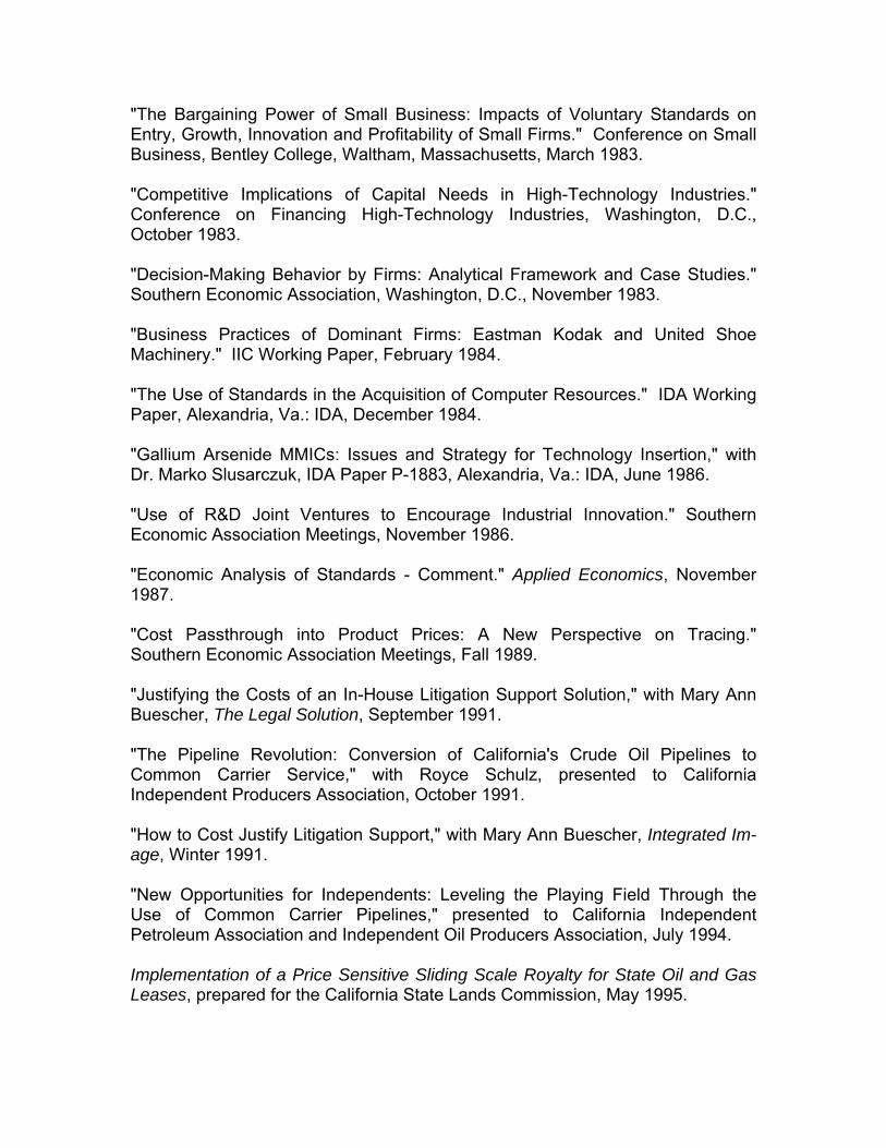
"The Bargaining Power of Small Business: Impacts of Voluntary Standards on Entry, Growth, Innovation and Profitability of Small Firms." Conference on Small Business, Bentley College, Waltham, Massachusetts, March 1983. "Competitive Implications of Capital Needs in High-Technology Industries." Conference on Financing High-Technology Industries, Washington, D.C., October 1983. "Decision-Making Behavior by Firms: Analytical Framework and Case Studies." Southern Economic Association, Washington, D.C., November 1983. "Business Practices of Dominant Firms: Eastman Kodak and United Shoe Machinery." IIC Working Paper, February 1984. "The Use of Standards in the Acquisition of Computer Resources." IDA Working Paper, Alexandria, Va.: IDA, December 1984. "Gallium Arsenide MMICs: Issues and Strategy for Technology Insertion," with Dr. Marko Slusarczuk, IDA Paper P-1883, Alexandria, Va.: IDA, June 1986. "Use of R&D Joint Ventures to Encourage Industrial Innovation." Southern Economic Association Meetings, November 1986. "Economic Analysis of Standards - Comment." Applied Economics, November 1987. "Cost Passthrough into Product Prices: A New Perspective on Tracing." Southern Economic Association Meetings, Fall 1989. "Justifying the Costs of an In-House Litigation Support Solution," with Mary Ann Buescher, The Legal Solution, September 1991. "The Pipeline Revolution: Conversion of California's Crude Oil Pipelines to Common Carrier Service," with Royce Schulz, presented to California Independent Producers Association, October 1991. "How to Cost Justify Litigation Support," with Mary Ann Buescher, Integrated Im-age, Winter 1991. "New Opportunities for Independents: Leveling the Playing Field Through the Use of Common Carrier Pipelines," presented to California Independent Petroleum Association and Independent Oil Producers Association, July 1994. Implementation of a Price Sensitive Sliding Scale Royalty for State Oil and Gas Leases, prepared for the California State Lands Commission, May 1995.

Impact of Electronic Data Interchange Technology on Small Business, U.S. Small Business Administration, July 1995. Crude Oil Marketing, prepared for U.S. Department of the Interior, Minerals Management Service, Valuation and Standards Division, July 1997. “Treasury Regulation 1.861: Interest Allocation Using Fair Market Value Methods,” Internal Revenue Service, CPE Seminars, August and September 2000. “Financial and Economic Indicators of Local Tax Burdens and Incentives to Invest in Various Localities,” November 2000. “Volatility in Gas Prices: Is it the Market or the Marketers?” Prepared for the U.S. Senate Permanent Subcommittee on Investigations, Committee on Governmental Affairs, May 2002. “Cost Sharing Regulations Embodied in the IRS Section 482 Transfer-Pricing Regulations: Recent Experience and Lessons Learned,” Internal Revenue Service, CPE Seminars, August 2002. “Heating Oil Prices in the Northeast: Haven’t We Been Here Before?” IIC, Inc. working paper, January 2004. Modeling Exploration, Development and Production in the Gulf of Mexico, U.S. Department of Interior, Minerals Management Service, Environmental Studies Program, Herndon, VA, OCS Study MMS 2—4-018, March 2004. The Impact of Tax Expenditure Policies on Incorporated Small Businesses, with Justin White, U.S. Small Business Administration, Office of Advocacy, Washington, D.C., April 2004. Trends in Electronic Procurement and E-Commerce and Their Impact on Small Business, with Mary Ann Buescher, June 2004. “Valuation of Intangibles under Section 482 of the Internal Revenue Code,” Internal Revenue Service, IVT Seminar, forthcoming June 2005. Testimony Before the U.S. Department of Energy, Office of Hearings and Appeals, Testimony on behalf of the States of Alabama et al., In the Matter of Cities Service Oil and Gas Corporation, HRO-0285, HRH- 0285, January and February 1987. Work performed on behalf of Lobel, Novins, Lamont, & Flug, Washington, D.C.

The People of the State of California, et al. v. Chevron Corp., et al., Case No. C-587912, Affidavits filed October 1986 and May 1990; oral testimony January 1993; January 1994; November 1994; April 1995; June 1999. Work performed on behalf of McMahon & Spiegel and Gibson, Dunn & Crutcher, Los Angeles, California. Richard A. Morhauser et al. v. Dori Shoe Company et al. Docket No. 85-102, Deposition and live testimony, September 1988 and February 1989. Work performed on behalf of Platz & Thompson, P.A., Lewiston, Maine. Robert N. MacDonald v. Stride Rite Corporation, Civil Action No. 88-0203P, Deposition testimony, June 1989. Work performed on behalf of Jackson, Lewis, Schnitzler & Krupman, New York, New York. John French et al. v. Robert Willman, Civil Action No. CV-89-83, Deposition and live testimony, June 1990 and October 1990. Work performed on behalf of Joseph A. Cloutier & Associates, Rockport, Maine. Exxon Corporation and Affiliated Companies et al. v. Commissioner of Internal Revenue, Docket No. 18618-89, 24855-89, 18432-90, Live testimony, April 1991. Work performed on behalf of the U.S. Internal Revenue Service, Dallas, Texas. Schott Motorcycle Supply, Inc. v. American Honda Motor Co., Inc., Civil Docket No. 90-0232P. Deposition Testimony, June 25-26, 1991. Work performed on behalf of Berman, Simmons & Goldberg, Lewiston, Maine. In Re: Coordinated Products Antitrust Litigation: All States Cases, MDL-150, CV-75-2232 AWT, Deposition testimony, June 16-17, 1992. Work performed on behalf of the States of California, Oregon, Washington, and Arizona, and Spiegel, Liao & Kagay, San Francisco, California. UNOCAL California Pipeline Co., FERC Proceeding, Docket No. IS92-18-000, Written testimony, August 1992. Work performed on behalf of Hoecker, McMahon, & Wade, Los Angeles, California. Chemoil Corp. v. Armstrong Petroleum Corp., Case No. 686767, Superior Court of California, Deposition Testimony, February 1993; Live testimony, May 1993. Work performed on behalf of Kelley, Drye & Warren, Los Angeles, California. City of Long Beach v. UNOCAL California Pipeline Co., CPUC Proceeding, Case No. 91-12-028, Written testimony, February 1993, Live testimony, March 1993. Work performed on behalf of Hoecker, McMahon, & Wade, Los Angeles, California.

The United States of America v. K.T. Derr, et al., Case No. C91-2872BAC, Live testimony, September 1993. Work performed on behalf of the U.S. Internal Revenue Service and U.S. Department of Justice. Market-Based Ratemaking for Oil Pipelines. FERC Proceeding, Docket No. RM94-1-000, February 1994. Work performed on behalf of Hoecker, McMahon & Wade, Los Angeles, California. Mission Resources, Inc.-II v. Texaco, Inc., et al., Case No. CVF-92-5850-REC, Deposition testimony, October 1993 and May 1994; Live testimony, June 1994. Work performed on behalf of Broad, Schulz, Larson & Wineberg, San Francisco, California. Judi Berry v. Harold Bilich, et al., Case No. CV-92-87, Deposition testimony, February 1994; live testimony, December 1994. Work performed on behalf of Cloutier, Barrett, Cloutier & Conley, Portland, Maine. Implementation of a Price Sensitive Sliding Scale Royalty for State Oil and Gas Leases, Testimony before the California State Lands Commission, May 1995. Application of Pacific Pipeline System, Inc., Prepared written testimony before the California Public Utilities Commission, May 1995. Work performed on behalf of Wright and Talisman, San Francisco, California. Farmland Industries, Inc. v. Commissioner of Internal Revenue, Docket No. 11881-93, Written and live testimony, May and June 1995. Work performed on behalf of U.S. Internal Revenue Service, Kansas City, Missouri. Nick C. Rini v. Robert N. Goldman, Docket No. 94-11367-PBS, Deposition and live testimony, February 1996. Work performed on behalf of Welte & Welte, Camden, Maine. Union Oil Company of California v. Pioneer Oil and Gas et al., Case No. SM92229, Deposition testimony, October 1996; Live testimony, January 1997. Work performed on behalf of McMahon & Spiegel, Los Angeles, CA. Blind Design, Inc. v. Hunter Douglas, Inc. et al., Case No. 686230, Deposition testimony, February 1997. Work performed on behalf of Sheppard, Mullin, Richter & Hampton, San Diego, CA. In the Matter of Beacon Oil Company, Contract No. DE-SC01-79-RA-32028, Deposition testimony, February 1997; trial testimony, March 1997. Work performed on behalf of the U.S. Department of Energy. State of Texas, et al. v. Amoco Production Co. et al., No. 95-08680, Deposition testimony, April 1997. Work performed on behalf of Susman Godfrey, L.L.P.

Execu-Tech Business Systems Inc., et al. v. Appleton Papers Inc., et al., Case No. 96-9639, CACE 05, Deposition testimony, September 1997; trial testimony, November-December 1997. Work performed on behalf of Heins, Mills & Olsen, Minneapolis, MN. Olde Port Mariner Fleet, Inc. Complaint re Casco Bay Island Transit District's Tour and Charter Service, Docket No. 98-161, prepared written direct and rebuttal testimony before the Maine Public Utilities Commission, July and September 1998. Oral testimony, October 1998. Work performed on behalf of Edward F. Bradley, Jr., Portland, ME. SouthPort Marine v. Boston Towing & Transport and Gulf Oil Corp., deposition and trial testimony, April 1999, work performed on behalf of Welte & Welte, Camden, ME and Flanagan & Hunter, Boston, MA. Northern Utilities, Inc. Petition for Waivers from Chapter 820, Docket No. 99-254, written testimony filed before the Maine Public Utilities Commission, May 2000. Work performed on behalf of Edward F. Bradley, Jr., Portland, ME. United States ex rel. J. Benjamin Johnson, et al. vs. Shell Oil Company, et al., Case No. 9:96CV66, expert reports and deposition testimony, February, May, and July 2000. Work performed on behalf of the Justice Department, Civil Division, Washington, D.C. Fidelity Oil Co. vs. Shell Western E&P Inc. and Shell Oil Co., Case No. DV-98-5817, expert reports, June 2001 and November 2001. Work performed on behalf of Crowley, Haughey, Hanson, Toole, & Dietrich, P.L.L.P., Billings, MT. Big West Oil Co. v. Frontier Pipeline Company and Express Pipeline Partnership and Chevron Products Company v. Frontier Pipeline Company and Express Pipeline Partnership, Docket Nos. OR01-02-002 and OR01-04-001, prepared direct testimony, November 2001. Worked performed on behalf of Goldstein & Associates, Washington, D.C. Big West Oil Company v. Anschutz Ranch East Pipeline, Inc. and Express Pipeline Partnership, and Chevron Products Company v. Anschutz Ranch East Pipeline, Inc. and Express Pipeline Partnership, Docket Nos. OR01-03-002 and OR01-05-001, prepared direct testimony, November 2001. Work performed on behalf of Goldstein & Associates, Washington, D.C. “Gas Prices: How Are They Really Set?” Hearings before the Permanent Subcommittee of Investigations of the Committee on Governmental Affairs, U.S. Senate, May 2, 2002.

Big West Oil, LLC, Chevron Products Company, and Tesoro Refining and Marketing Company v. Express Pipeline LLC and Platte Pipe Line Company, Docket No. OR02-5-000; Big West Oil, LLC, Chevron Products Company, Sinclair Oil Corporation and Tesoro Refining and Marketing Company v Express Pipeline LLC, Docket No. OR02-8-000; Big West Oil, LLC, Chevron Products Company, and Tesoro Refining and Marketing Company v. Platte Pipe Line Company, Docket No. IS02-384-000. Prepared direct and answering testimony, March 27, 2003. Worked performed on behalf of Goldstein & Associates, Washington, D.C. Sinclair Oil Corporation v. BP Pipelines (N.A.), Inc., Docket No. OR02-6-02; Prepared direct testimony, September 2003; rebuttal testimony, March 2004. Work performed on behalf of Goldstein & Associates, Washington, D.C. Public Hearing on Property Tax Classification, Hearings before Massachusetts Department of Revenue, May 2004, direct testimony on proposed modification to state property tax classification system. Marc Leslie and Mary Leslie v. Winslow Marine, Inc., Docket No. BATSC-CV-2003-00031; Deposition testimony, February 2005. Work performed on behalf of Tompkins, Clough, Hirshon and Langer, P.A.