REPORT DOCUMENTATION PAGE FINE SEDIMENT REGIME...

REPORT DOCUMENTATION PAGE1. Report No. 2. 3. Recipient's Acceslion No.

4. Title end Subtitle 5. Report Date

FINE SEDIMENT REGIME OF LAKE OKEECHOBEE, FLORIDA -November 19896.

7. Author(s) Robert R. Kirby 8. Perfortin Orsanization Report No.Carl. H. HobbsAshish J. Mehta UFL/COEL-89/009

9. Performing Organization Name and Address 10. Project/Task/Work Unit No.

Coastal and Oceanographic Engineering Department Lake Okeechobee PhosphorusUniversity of Florida Dynamics Study. Task 7

336 Wel Hall 11. Contract or Crant No.336 Well HallGainesville, FL 32611

13. Type of Report12. Sponsoring Organization Name and Address

South Florida Water Management District FinalP.O. Box V, 3301 Gun Club RoadWest Palm Beach, FL 33402

14.

15. Supplementary Notes

16. Abstract

The purpose of the study reported herein was to characterize the sediments of LakeOkeechobee through field and laboratory studies, with special emphasis on the fine sedi-ment regime. Continuous seismic profiling information, involving side-scanning and shallowreflection apparatus, was obtained. Despite the exceptionally shallow water depths in thelake, compounded by the presence of gas in the superficial muds, good quality data revealingthe lake bed stratigraphy and indicating suitable sites for later sampling were derived. Thesampling program was designed to establish the complete succession with special emphasison the superficial muds. The underlying geological bedrock succession is consistent in termsof overall thickness and numbers of thin calcareous deposits with that already establishedonshore.

Overlying the bedrock, around the southern and northeastern periphery at least, is athick in situ peat bed. The peat dates from 5,490 yr BP to 2,670 yr BP, a time when proto-Lake Okeechobee had a much more restricted extent than at present. Extending over muchof the northern part of the lake and overlying the peat in places is a thin fan of quartz sand.The sand is most recently of fluviatile origin and its extent and variation in thickness implyinput by streams and rivers from the north.

- Continued -

17. Originator's Key Words 18. Availability Statement

Bottom characterizationFine sedimentLake mudLake Okeechobee

19. U. S. Security Classif. of the Report 20. U. S. Security Classif. of This Page 21. No. of Pages 22. Price

Unclassified I Unclassified 77

The shallowest deposit and the one of greatest interest in respect of nutrient cycling inthe lake is a black, carbonate and organic rich mud. As with the sand, the mud is restrictedto the northern end of the lake, occupying about one third of the area of the lake bed. Itcontains - 193 x 10 6 m3 of material and is offset slightly to the northeast of the central deepof the lake. As a result its surface slopes towards the southwest at a low angle. Mud depthsrange from a few centimeters at the periphery to in excess of 75 cm in the deep center ofthe lake. The deposit has been accumulating for a long period (~ 6300 yr). Its distributionsuggests input of some components from the same northern rivers which supplied the sand.Variation in deposition rate with time remains to be investigated.

Internally the deeper, central mud area shows slight lithological variations interpretedto imply that deposition commenced here. The upper and more extensive part of the mudsuccession looks less differentiated in cut section, but high resolution X-radiography of thinvertical slices showed that the lower horizons exhibit a microscopic interlamination of darkand light bands, thought to arise from periods of algae blooming, death and sedimentation ofskeletal debris, alternating with more normal periods of deposition of organic floc material.The microscopic internal primary fabric is clear evidence that the deeper layers of the mudpatch are not susceptible to frequent reworking. The X-radiographs also show that thereappear to be spherical gas bubbles in the mud in some areas.

In situ density profiles of the upper part of several cores revealed a relatively thin (0-10cm), fluid mud veneer. This material is believed susceptible to resuspension on occasions.Between the submillimeter lower zones and the top-most fluid mud upper zone is often abroad (up to 25 cm) zone apparently with poorly developed internal primary fabric. Thiszone is slightly problematical because whereas shear strength profiles imply the zone to betoo strong to be regularly resuspended, the presence of gas within the zone could lead toconsiderably enhanced susceptibility.

The present results need to be considered along with the nutrient profile data to assistthe understanding of the relationship between sediment entrainment and nutrient cycling.It is concluded that the role of gas merits further close scrutiny.

UFL/COEL-89/009

FINE SEDIMENT REGIME OF LAKE OKEECHOBEE,FLORIDA

by

Robert R. KirbyCarl H. HobbsAshish J. Mehta

Sponsor:

South Florida Water Management DistrictP.O. Box V, 3301 Gun Club RoadWest Palm Beach, FL 33402

November, 1989

UFL/COEL-89/009

FINE SEDIMENT REGIME OFLAKE OKEECHOBEE, FLORIDA

Robert R. KirbyCarl H. Hobbs

Ashish J. Mehta

Coastal and Oceanographic Engineering DepartmentUniversity of FloridaGainesville, FL 32611

November, 1989

ACKNOWLEDGMENT

This investigation was conducted as a part of the Lake Okeechobee Phosphorus Dynamics

Study funded by the South Florida Water Management District, West Palm Beach, Florida

(SFWMD). The authors wish to acknowledge Brad Jones and Dave Soballe of SFWMD

for their assistance and Dr. Ramesh Reddy for coordinating the University of Florida team

effort. Acknowledgement is also due to Dr. Andrew Salkield and Prof. Paul Visser for

their participation in some of the field effort. Thanks are extended to the staff of the

Coastal Engineering Laboratory, particularly Sidney Schofield, whose field study planning

and coordination effort were critical to project execution. Graduate Assistant Xueming Shen

carried out laboratory core analysis.

ii

TABLE OF CONTENTS

ACKNOWLEDGMENT ........................................ . ii

LIST OF FIGURES ..................................... v

LIST OF TABLES . .................. ... .............. . vii

SUM MARY ... ........ .... .................... .......... viii

1 INTRODUCTION 1

2 METHODS 3

2.1 Field Techniques .................. .................. 3

2.2 Laboratory Techniques .............. .................. . 7

3 RESULTS 15

3.1 Introductory Note .................... .............. . 15

3.2 Geophysics ........ .......................... .. ...... 15

3.3 Samples .................. ................... .... 18

3.3.1 Beach rock ..... .......... ................. ...... 18

3.3.2 Peat .................. .... .......... ..... .... . 20

3.3.3 Sand .. ...... .................................. 20

3.3.4 Mud . ........... ...... .. ................ .. . . 21

3.3.4.1 X-radiography ....... ..... ..... .. ............ ........ 24

3.3.4.2 Evidence of Gas in Mud Deposits . ........... . .......... . 26

3.3.4.3 Density and Shear Strength Profiles . . . . . . . . . . . . . . ... . . .. . . . 27

3.3.5 Problematic Substrate ................... ............ 29

4 GEOLOGICAL STRUCTURE 32

5 RECOMMENDATIONS FOR FURTHER WORK 35

6 CONCLUSIONS 37

7 REFERENCES 39

APPENDICES

A REPORT ON GEOPHYSICAL FIELD OPERATION 40

A.1 Introduction ....................................... 40

A.1 Side-scan Sonorgraphy ..... ...................... ..... 50

A.1 Sub-bottom Profiles .......... .... . ... ..... ..... ..... . 51

iii

B REPORT ON CORING SURVEY 57

B.1 Field Operation .................... ................. 57

B.2 Apparatus . .................... ... ................ 57

B.3 Itinerary . . . . . . . . . . . . . . . . . . . . . . . . . . . . . . . . . . . . . . . . . 59

B.4 Equipment Performance .................... ............ 59

C SAMPLE CORE DESCRIPTIONS 61

C.1 Site: OK9 VC ................... .................. . 61

C.2 Site: OK10 VC ..................... ............... . 63

C.3 Site: OK18 VC ..................... ............... . 64

C.4 Site: OK31 VC ..................... ............... . 64

D SEDIMENT SAMPLING IN SPRING, 1988 65

iv

LIST OF FIGURES

1 Bathymetric map of Lake Okeechobee. Depths are relative to a datum which is

3.81 m above msl. ................ . ... . ............ 4

2 Vibracorer being deployed for core collection. . . . . . . . . . . . . . .... .... 6

3 Core OK1 VC. ..................................... 8

4 Core OK2 VC. ...................................... 9

5 Core OK11 VC . . . . . . . . . ........ . . . . . . . ...... . . . . .. 10

6 Vibracore sampling locations. . . . . . . . . . . . . . . ... ............ .. 11

7a Core X-radiograph. X-ray (7 kv; 550 ma) exposure time was 2 seconds. Lower

part of core OK1 VC. Nail image is 5.1 cm in length. . . . . . . . . . . . ... . 12

7b Core X-radiograph. X-ray (7 kv; 550 ma) exposure time was 2 seconds. Upper

part of core OK1 VC. Nail image is 5.1 cm in length. . . . . . . . . . . . ... . 13

8 X-radiograph of core OK11 VC .. ................. ......... 14

9 Surface sediment distribution in Lake Okeechobee including coring grid pattern

(courtesy Ramesh Reddy and Don Graetz, UF Soil Science Department).

Compare with sediment distribution map produced in this study (Fig. 10). .16

10 Sediment distribution map of Lake Okeechobee. . . . . . . . . . . . . . . . .... 19

11 Mud thickness contour map of Lake Okeechobee. . . . . . . . . . . . . . . . ... 23

12 Mud vane shear strength variation with density (after Hwang, 1989). ...... ... 30

13 Schematic showing velocity and concentration fields under wave action and sug-

gested instrumented tower. ................... ......... 30

A.1 Geophysical lines with measurement time markers. . . . . . . . . . . . . . .... 41

A.2 Portion of side-scan record, line 2, October 12, 1988, west-east. . . . . . . . ... 52

A.3 A portion of Line 9 demonstrating a shelly (?) mud layer approximately 60 cm

thick over a harder substrate. The deeper sub-bottom reflector depicts a small

paleochannel ................... ................ . 53

A.4 A portion of Line 4 demonstrating a relatively clean mud layer over a harder

substrate. The sub-bottom reflector depicts a small paleochannel showing

signs of some internal compaction. . . . . . . . . . . . . . . ... ....... 54

A.5 A portion of Line 4 depicting a somewhat shelly (?) mud layer overlying a harder

substrate. The relatively shallow sub- bottom reflector dips toward the right. 55

A.6 A portion of Line 6 depicting both the 7 KHz and 200 KHz bottoms. The

roughness of the bottom surface is due to surface water waves approximately

0.5 m high. The strength of the multiples of the 7 KHz bottom suggests that

the bottom is relatively hard ................... ....... . 56

C.1 Core descriptions: a) OK9 VC, b) OK10 VC, c) OK18 VC, d) OK31 VC. . . . . 62

V

D.1 Sediment/core sampling sites in Spring, 1988. . . . . . . . . . . . . . . . .... . . 66

D.2 Frozen core from site 1 ................................ 67

vi

LIST OF TABLES

3.1 Core/Clamshell Sample Description ................. . ....... .. 28

4.1 Lake Okeechobee Deposit Sequence . . . . . . . . . . . . . . ..... ........ . 32

A.1 Latitude and Longitude as Displayed by Micrologic 7500 LORAN- C ...... .. 42

A.2 Summary of Track Lines ................... . ............ 50

D.1 Bed and Sediment Characteristics . . . . . . . . . . . . . . ..... ........ . 68

vii

SUMMARY

The purpose of the study reported herein was to characterize the sediments of Lake

Okeechobee through field and laboratory studies, with special emphasis on the fine sedi-

ment regime. Continuous seismic profiling information, involving side-scanning and shallow

reflection apparatus, was obtained. Despite the exceptionally shallow water depths in the

lake, compounded by the presence of gas in the superficial muds, good quality data revealing

the lake bed stratigraphy and indicating suitable sites for later sampling were derived. The

sampling program was designed to establish the complete succession with special emphasis

on the superficial muds. The underlying geological bedrock succession is consistent in terms

of overall thickness and numbers of thin calcareous deposits with that already established

onshore.

Overlying the bedrock, around the southern and northeastern periphery at least, is a

thick in situ peat bed. The peat dates from 5,490 yr BP to 2,670 yr BP, a time when proto-

Lake Okeechobee had a much more restricted extent than at present. Extending over much

of the northern part of the lake and overlying the peat in places is a thin fan of quartz sand.

The sand is most recently of fluviatile origin and its extent and variation in thickness imply

input by streams and rivers from the north.

The shallowest deposit and the one of greatest interest in respect of nutrient cycling in

the lake is a black, carbonate and organic rich mud. As with the sand, the mud is restricted

to the northern end of the lake, occupying about one third of the area of the lake bed. It

contains ~ 193 x 10 6 m3 of material and is offset slightly to the northeast of the central deep

of the lake. As a result its surface slopes towards the southwest at a low angle. Mud depths

range from a few centimeters at the periphery to in excess of 75 cm in the deep center of

the lake. The deposit has been accumulating for a long period (- 6300 yr). Its distribution

suggests input of some components from the same northern rivers which supplied the sand.

Variation in deposition rate with time remains to be investigated.

viii

Internally the deeper, central mud area shows slight lithological variations interpreted

to imply that deposition commenced here. The upper and more extensive part of the mud

succession looks less differentiated in cut section, but high resolution X-radiography of thin

vertical slices showed that the lower horizons exhibit a microscopic interlamination of dark

and light bands, thought to arise from periods of algae blooming, death and sedimentation of

skeletal debris, alternating with more normal periods of deposition of organic floc material.

The microscopic internal primary fabric is clear evidence that the deeper layers of the mud

patch are not susceptible to frequent reworking. The X-radiographs also show that there

appear to be spherical gas bubbles in the mud in some areas.

In situ density profiles of the upper part of several cores revealed a relatively thin (0-10

cm), fluid mud veneer. This material is believed susceptible to resuspension on occasions.

Between the submillimeter lower zones and the top-most fluid mud upper zone is often a

broad (up to 25 cm) zone apparently with poorly developed internal primary fabric. This

zone is slightly problematical because whereas shear strength profiles imply the zone to be

too strong to be regularly resuspended, the presence of gas within the zone could lead to

considerably enhanced susceptibility.

The present results need to be considered along with the nutrient profile data to assist

the understanding of the relationship between sediment entrainment and nutrient cycling.

It is concluded that the role of gas merits further close scrutiny.

ix

1 INTRODUCTION

Lake Okeechobee provides many functions for south-central Florida, including drainage,

water supply, flood relief and recreation. The water quality of the lake has deteriorated

over thirty years or more as evidenced by its chemical and biological properties. During this

period farming practices and various other changes in the lake's watershed have occurred.

Should water quality continue to decline, it is likely that plankton blooms will become more

extensive, frequent and severe with the ultimate threat of eutrophication of the system.

Steps need to be taken to reduce nutrient input to the system, but at present the major

factors influencing the deteriorating water quality are not well documented or understood.

One scenario envisages that increasing input of nutrient to the inflowing waters are

largely or entirely responsible for deteriorating water quality and that steps need to be

taken to reduce these. Should this turn out to be the case, it requires a clearly defined

course of action. A different scenario, however, envisages that, notwithstanding present

nutrient loads, a large proportion of nutrients are sorbed onto fine sediment particles, which

are periodically resuspended leading to partial nutrient release. According to this internal

loading dependent scenario, decreasing the fresh nutrient input will have little short-term

impact, because nutrient releases will continue to be dominated by fine sediment entrainment

and nutrient leaching.

The study reported here is aimed at characterizing the bottom sediment regime in the

lake. This has been approached by undertaking a continuous seismic profiling survey followed

by a coring survey to characterize the various acoustic reflectors recognized by the geophysical

instruments. The coring survey involved sampling with a small hand-held vibracorer. The

vibracorer permitted the complete succession to be penetrated, except where indurated rock

is exposed directly at the lake bed. The undisturbed samples were returned to the Coastal

Engineering Laboratory at the University of Florida (UF) for the following sedimentological

and geophysical testing to characterize the deposits. a) cutting, preparation and photography

to determine the sedimentary succession, b) measurement of down-core density and shear

1

strength profiles to determine erosion potential, and c) cutting of thin slices from the axis

of cores for X- radiography to show the primary sedimentary fabric of mud deposits.

In addition to these laboratory studies, where very loosely consolidated "fluid mud" type

deposits were observed to overlay the more consolidated muds in the field, in situ density

profiles of these top-most deposits were performed on board ship at the time of collection

with a vibrating tube-type densimeter. Such in situ measurement was essential as the loosely

consolidated fluid mud deposits would otherwise have dewatered during transport and been

impossible to measure in the laboratory.

Some of the measurements carried out under this study, e.g. core density and shear

strength measurements, were also useful to a companion study on lake sediment resuspension

and deposition (Hwang, 1989). Those measurements therefore are reported in detail in that

study and only summarized in what follows.

2

2 METHODS

2.1 Field Techniques

Classical geological/sedimentological investigations of the type required in this study de-

mand application of a particular suite of techniques which must be deployed in a set order.

Firstly, continuous seismic profiling techniques must be applied. These include two basic

types of instruments. A side-scan sonar allows the surface topography and acoustic char-

acter of sediments exposed at the lake bed to be mapped. At the same time, penetrating

acoustic devices of some kind must be deployed to map the subsurface reflectors. See Ap-

pendix A for a report on the geophysical field operation.

The maps prepared from these two types of system then provide the input and basis upon

which sample localities are chosen to characterize each reflector type and the sedimentary

succession. Arising from this heirachy of techniques it is clearly essential to complete the

geophysical surveys before moving on to the bottom sampling program.

In this case the extremely shallow nature of the lake (maximum depths 4-5 m depending

on water level, see Fig. 1), together with the suspected presence of gas in the sediments,

imposed certain requirements upon the type of seismic device used. Arising from its known

high resolution it was decided to use an E.G. & G side-scan sonar. The extremely shallow

water depth and mud layer thickness indicated that a short pulse-length, variable frequency

pinger was the best high-resolution, shallow-penetration device to chose. By the use of these

devices continuous seismic profiles of a better caliber than any previously available from the

lake have been obtained.

The E.G. & G SMS-960 side-scan sonar employs a towed torpedo-shaped fish with 105

kHz transducers on either side. It produces a fan- shaped pulse of sound (in the vertical

plane with the transducer forming the axis or hinge of the fan). Foreward movement of the

fish ensures that successive strips of the bed are scanned. By this technique two swathes of

the lake bed extending from directly under the survey vessel out to a nominal range of

3

271 ..' 2 3.0'81 00 .1 3 8040

N '. I

26:4§" 2

I\ 1

2

80 40+' , 26045'S80°40

0 5sKm Dbepths In MetersBelow Datum

Fig. 1. Bathymetric map of Lake Okeechobee. Depths are relative to adatum which is 3.81 m above msl.

4

100 m on either side are covered. The E.G. & G SMS-960 employs a signal conditioning unit

which produces digital records are scale corrected to provide an undistorted image.

The Datasonics SBP-5000 pinger employs a piezo-electric crystal to produce the acoustic

pulse which is directed down through the lake bed. A receiving hydrophone collects the

returning acoustic signals from sub-surface reflectors. In addition to the variable frequency

(3.5, 5 or 7 kHz) pinger a high frequency (200 kHz) echo sounder was operated in parallel.

The high and low frequency systems are complementary, permitting precise bottom tracking

and good penetration, respectively.

To complete the mapping a small mechanical vibracorer was developed and deployed

from a davit on the UF research vessel Silver Bullet. The vibracorer basically has a concrete

vibrator powered through a flexible drive from a gasoline motor on board the survey vessel.

The concrete vibrator was clamped onto the top of the drill barrel. The drill barrel was

1.83 m in length and had an i.d. of 9.4 cm. It was fitted with a transparent liner to contain

the sample. To permit core penetration and retention, a steel cutting shoe, plastic, petal-

type core catcher and a non- return valve were fitted. A threaded collar on the top of the

corer permitted a guide tube to be fitted. This was attached after the vessel had anchored

and the corer had been hung over the side and into the water. The guide tube allowed the

vertical position of the corer to be maintained during drilling operations (Fig. 2) as well

as permitting visual monitoring of bed penetration. Sample sites were chosen at localities

where the geophysical records indicated that particular topographic or lithological features

occurred at the surface or within reach of the vibracorer, but below the mud surface. See

Appendix B for a brief report on coring survey.

On recovering the vibracorer, the transparent liner was capped at its base and removed

from the core barrel. The sample was then measured and described on board ship. In

circumstances where the upper surface of the mud deposits was very loosely consolidated

a Paar (DMA 35) densimeter was used in the field to measure the density structure of the

upper, lowly consolidated horizons. The Paar densimeter is a small, battery operated device

5

Fig. 2. Vibracorer being deployed for core collection.

6

for accurate measurement of the density of slurries. It operates on the principle of a vibrating

glass U-tube. The frequency of the vibration is directly influenced by the slurry, which is

converted to density in the instrument and displayed digitally. The core liner was then

capped at the top and numbered before being stored in an upright position for transport to

the laboratory.

2.2 Laboratory Techniques

In the laboratory the cores were laid in a clamp and the liner only was cut down opposite

sides with an electric saw. The core was then halved by drawing a cheese wire down the cuts

and through the sample. The bisected core was then opened so that both halves could be

described and photographed. Illustrative core photographs are included in Figs. 3, 4 and 5.

Core locations are shown in Fig. 6.

No further studies were made on quartz sand, peat or beach rock, but attention was

concentrated on the upper muddy zone, where this was present. Shortly after cutting and

before the sample could dry to any extent, vertical profiles of density and shear strength

were made.

The density profiles were made gravimetrically and the shear strength profiles were mea-

sured with a small calibrated vane (Wykeham Farrance, Model 100). Cone penetrometer

tests were also carried out. Measurements were made at 5 cm increments of depth and the

vane was inserted sideways into the axial (thickest) part of the halved core. This procedure

disrupted the sample, rendering it inappropriate for later non-destructive testing.

The other half of the core was then tipped gently out of the liner to rest with its diameter

flat on a board. The upper, curved section was then removed with the cheese wire and

a palette knife to leave behind a constant thickness (5 mm) undisturbed slice from the

maximum diameter of the core. This slice was then X- radiographed using a standard X-ray

machine with a low powered (75 kV, 550 mA) head. The X-ray films were then processed

to show the very small scale and detailed primary fabric of the mud layers. Illustrative

examples are shown in Figs. 7a, 7b and 8.

7

OKI

vc

Fig. 3. Core OK1 VC.

8

.+* ) . .,


0

OK

11

VC


10

27' 0' \ 27010'81000,' 180040'

k ... -31T - 20 0 19 18

N 2

.A 3

.1 /* *46'5 , 3 0

8 7 6 29 5

17 16 15 14

9 10 28\*

12 13

C', 25 24 23 22 21

26 27

2604265'80040 126-45'180040'

0 5Km

Fig. 6. Vibracore sampling locations.

11

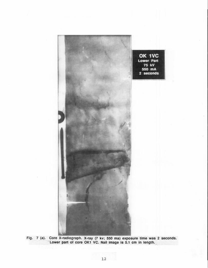
Fig. 7 (a). Core X-radiograph. X-ray (7 kv; 550 ma) exposure time was 2 seconds.Lower part of core OK1 VC. Nail mage is 5.1 cm in length.

12

P F_

Fig. 7 (b). Core X-radiograph. X-ray (7 kv; 550 ma) exposure time was 2 seconds.Upper part of core OK1 VC. Nail Image is 5.1 cm in length.

1il

Fig. 8. X-radiograph of core OK11 VC.

14

3 RESULTS

3.1 Introductory Note

Part of the task of characterizing the sediments is to map their areal and vertical extent.

A map showing the surface sediment distribution is presented as Fig. 9; illustrative core

descriptions are provided as Appendix C. For all core descriptions see Hwang (1989). These

form the basis upon which the geological history is established.

3.2 Geophysics

Sub-bottom profiles were of variable quality, possibly being strongly influenced by weather

conditions experienced during the survey. Some records, i.e. those from lines 2, 3 and

especially Line 4, were particularly good.

The geological history revealed by the continuous seismic profiling records is of well

defined, if shallow, limestone (?) bedrock basins or swallow holes. In the north the basins

are separated by a N-S orientated narrow ridge, which finds no surface expression today.

Further south it appears that the bedrock rises westwards and reaches the lake bed. The

extent and number of the basins is difficult to establish owing to the variable record quality.

The origin of the basins is not clear from the geophysics records alone. In addition to

these series of basins the bedrock surface, at least in the west on Line 4, where record quality

was excellent, is quite irregular and shows a large number of steep, often V- shaped, valleys

or channels which criss-cross the margin of the basin. Similar channels are also incised into

the bed of the basin. The abundance and shape of the channels gives rise to the tentative

suggestion that they may be infilled, possibly tidal, channels.

More recent calcareous deposits overlie much of this ancient topography with the result

that the more accentuated, if low, relief has become muted. In the basins themselves the

overlying calcareous deposits are generally of a sheet-like and extensive nature. In the more

central areas of the lake up to 5 separate layers can be resolved, whereas towards the edge

of the lake it is generally the case that only two layers are present. The depth of the

15

K L1M

;i::.. N

* .* o

G0 F 0 ;*

. . .. ..

o ,t, T ooI4r, . .J. "" -

.... . . . C.,

0. MARSH......

SI, .-D/,H

SMUD

SROCK/MARL

Fig. 9. Surface sediment distribution in Lake Okeechobee including coring gridpattern (courtesy Ramesh Reddy and Don Graetz, UF Soil Science Department).Compare with sediment distribution map produced in this study (Fig. 10).

16

deposits ranges up to a maximum of 4 m, but is more generally in the range 1.5 - 2.5 m.

The complex history of the deposits is illustrated from the fact that deeper layers of these

calcareous rocks are themselves cross-cut by later channels and the channels, in turn, have

been infilled. Apparently a similar environment to that under which the basins and their

incised channels were formed existed during the later period when the basins were becoming

infilled by the calcareous layered deposits.

The vibracorer nowhere reached down more than 30-40 cm into these indurated calcareous

rocks, which are referred to here by the generic term "beach-rock." The highly cemented

nature and presence of marine shell species in samples (e.g. see Fig. 7a) suggests they are

likely to be in part old shallow marine sediments of possible Plio-Pleistocene age. As a result

the deeper layers remain unexplored, other than by these seismic techniques.

Overlying mud deposits are difficult to isolate from the underlying beds on the geophysics

records. Signals from the mud zone are often "acoustically turbid" - possibly indicating the

presence of dispersed gas. At some sites deep-lying strong reflectors may be from shelly

layers, e.g. on Line 7 in the south. Elsewhere, for example on Line 4, in addition to the

acoustic turbidity the signal from the upper horizon showed strong surface or near-surface

reflectors and a phase reversal of the signal. Initial inspection might suggest the presence of

coral boulders at the surface, but the 200 kHz record clearly showed a planar lake bed and

the parabolic reflectors diagnostic of rock debris are absent from the record. Instead it seems

more likely that these signals are due to the presence of gas accumulations in the sediment.

This is also suggested by the weak reflectance of the surface seen on the side- scan records.

These zones of phase reversal are at times several tens of meters in extent on the pinger

records and would undoubtedly be picked up on the side-scan records if there were patches

of shell or rock at the surface. The side-scan records did, however, show a multitude of

small (< 1 m) point-source strong reflectors at the lake bed (see e.g. Fig. 7a). These strong

reflectors could have several origins.

To investigate the character of the unconsolidated sediments at the lake bed and interpret

the geophysics, samples had to be taken.

17

3.3 Samples

The accessible part of the geological succession is rather straightforward. The entire lake

appears to be founded on a whitish, calcareous marine "beach rock" type material. Almost

all cores penetrated into this although in some cases, especially in the south, the beach rock

is so indurated that the vessel could either not anchor or the corer was unable to penetrate.

In a few cases the deposits overlying the beach rock are sufficiently difficult to drill and have

a thickness such that they were not completely penetrated by the corer. Over part of the

area the beach rock is overlain by a peat layer. Above the peat and not quite coincident with

its preservation is a quartz-sand horizon. The shallowest deposit is a blackish, organic-rich

clay layer, which shows both macroscopic and microscopic primary layering. The peat, sand

and mud occur chiefly at the northern end and in the center of the lake, whereas the southern

end is largely free from unconsolidated sediment. The extent and thickness of the various

horizons are shown in the bed sediment distribution map (Fig. 10).

Much of the margin of the lake, especially on the west side, is extremely shallow and

difficult to gain access to as a result of extensive beds of vegetation. This zone could not be

investigated during this survey, but has been investigated by UF's Soils Science Department

in a companion study. The various formations are discussed in the following sections.

3.3.1 Beach rock

A cemented calcareous white deposit forms the basement of the lake, being exposed

at the lake bed for up to 50% of its area. These deposits are of variable lithology and

include indurated lime muds, nodular limestones, calcareous sands and sandstones and shelly

horizons. In places the upper zone shows signs of weathering and the penetration by rootlets

from the overlying peat. The shelly fauna consists of gastropod and bivalve species and has

not been specifically identified. These basal deposits were considered by Gleason and Stone

(1975) and Brooks (1984). The calcareous deposits are probably the complete succession of

the Caloosahatchee-Fort Thompson formation (Plio-Pleistocene).

18

Okeetantier NW

127 \ Marina/'20 7«'

/ o7 : :?. 4

0

8i•oiT6 o- -- 14A'

,, /17 \ W9? Z X .. - a a

Lakeport -30 28

0-

2 : rPortMayaca

24 5 ---- . -"R ,

25 23 2. 2 2)R.

S .-- .- ..* 4 ..- .-- -I

; - r12 0 '

S269? OR oR OR1

Moore Heaven

ORr ePahokee

o80401 Clewiston e80os40'

0 s-m

Depths in Motors8elow Datum

Bathymetry-depth in feet23 Core Stationo Beach Rock in Core

oR Beach Rock at Surface, not Sampled

P Peat in Core or Outcropping at SurfaceConjectured Extent of Peat Deposit

X Quartz Sand--- 0 Marginof Sand Area

--- 40 Sand Patch > 40cm deep[] Black Mud

-. 0.-- Marginof Mud Area----- 30 Mud Patch > 30cm deep---- 60 MudPatch > 60cm deep

? Possible Bed Rock? Possible FuvialSand

Fig. 10 Sediment Distribution Map of Lake Okeechobee.

1919

3.3.2 Peat

One of the more unexpected discoveries of the sampling campaign is the depth and geo-

graphical extent of peat deposits at the northern end of the lake. The authors are not aware

that peat deposits have been recognized at the northern end of the lake before.

The peat deposits are believed to lie in situ. In a number of cases the beach rock

upon which they invariably rest is penetrated by rootlet beds from the vegetation which

originally grew upon the beach rock surface. The fact that the peat is in places layered

and shows a variety of textural features may also support the view that it is in situ and

if the need arose could be sampled for pollen and other evidence of the past environment

around Okeechobee. The relatively thick and layered peats hint at a quite prolonged period

of sub-aerial exposure during which a variety of climatic or environmental changes occurred.

No attempt was made in this study to carry out pollen dating, radiocarbon dating or any

identification of macroscopic plant remains.

Being organic, peat layers are known to generate and hold gas. As such they present

particular difficulties to seismic devices, which generally will characterize them as strong

reflectors, producing a phase reversal of the acoustic signal. Peat layers are thus difficult for

seismic devices to "see through" to what is underneath. In this case what is below is the

beach rock and is of little direct interest to this study.

The extent of the peat suggests that at some stage the entire basin may have been a peat

bog or at least that the water may have occupied a smaller area in the deep center of the

present lake. The oldest previously known peats are 5,490 yr BP and range up to 2,670 yr

BP (Gleason and Stone, 1975).

3.3.3 Sand

In those few cores where the succession is complete the peat is overlain by a grayish

quartz sand. The sand occupies a broader zone than the peat at the northern end of the

lake, although it is generally thin (< 10.0 cm). Only around the entrance to the Kissimmee

20

River does its thickness increase (40-50 cm). Here a series of sand layers with differing grain-

sizes and shell content overlie each other. In the west the sand layers are exposed at the lake

bed and not entirely covered by the more recent black muds.

The northern distribution of the sand patch and the fact that it is thickest in the proximity

of the Kissimmee River, combined with the fact that it overlies the terrestrial peat, are all

indicative of a fluviatile sand supplied by the Kissimmee River drainage basin, as opposed

to a marine beach sand.

At the southern extremity of the fan of sand thin sand layers are interbedded with the

overlying black muds at two sites. This suggests that the sand sheet originally had a rather

greater southerly extent and was reworked back onto the proximal mud deposits at a much

later date.

The sand layer is indicative of a change in source rocks or deposits in the hinterland

compared to that which is presently supplied. The Kissimmee River watershed constitutes

more than 50% of Okeechobee's drainage basin and the Plio-Pleistocene deposits are more

sandy in the north. The sand layer is not directly relevant to the present investigation.

3.3.4 Mud

Black, organic-rich muds form an extensive veneer in the northeast quadrant of the lake,

possibly covering a third of the entire bed. Why the mud should be absent from the southern

end and western sector of the lake is unclear, especially because the western side of the lake is

heavily vegetated and thus provides both more sheltered and possibly more nutrient enriched

waters. Possibly the distribution is linked in some way with inputs of nutrients or inorganic

fine sediment from Taylors Creek or the Kissimmee River in the north. Equally it is not

immediately apparent why the mud is absent in the south, other than to observe that the

distribution of sand and mud are similar in this respect. Maps showing both bathymetric

contours and the extent of the mud patch (Figs. 1 and 10) reveal that the mud patch is offset

to the north-east such that its surface is inclined to the south-west. This is presumed to

reflect a hydrodynamic control. The mud layer is generally less than 30 cm thick, although

21

in two areas it exceeds 30 cm and approaches 75 cm in one. The area of maximum thickness

of mud is almost coincident with the area of deepest water, possibly indicating a link.

The general outline of the edge of the mud patch is closely coincident with that mapped in

greater detail with more samples by UF's Soil Science Dept. (Fig. 9). Most discrepancies are

comparatively minor and probably accounted for by the poor repeatability of the LORAN

positioning system (see Appendix A), added to the fact that the mud area thins to a feather

edge at its margins and probably is patchy. There is a greater discrepancy in the south where

seven stations were attempted during this survey. At five the vessel could not anchor or the

vibracorer would not penetrate, indicating the presence of rock at the surface. The anchors

came up clean. At the remaining two stations the corer produced rock samples. Clearly any

black mud here must be thin and very soft. The southerly limit of mud is probably about

260 54'N whilst the Soil Sciences map shows a greater southerly extent down almost to 260

49'N.

Whereas the boundary of the mud area as mapped by Soil Sciences and this vibracoring

survey are generally coincident the thickness of the mud patch sometimes appeared rather

different. This is largely accounted for by the fact that Soil Science mapped the mud depth

by measuring core length in the field. In contrast, in this study the length is measured from

opened cores. The peat and sand layers omitted from this study result in a smaller mud

thickness. To facilitate core retention the vibracorer used a petal-type core catcher. In the

very lowly consolidated muds encountered this could have given rise to a certain amount of

loss at the top of the sample. Other evidence (below) shows that the amount of disturbance

caused to the sample by the vibration, core-catcher, recovery or removal and capping of the

core was, however, generally slight. In Fig. 11, a mud contour map is presented to highlight

the variability of mud thickness. This variability appears to be considerably greater than

that suggested by Gleason and Stone (1975), although their observations regarding mud

distribution in the lake are confirmed in a qualitative sense. Four sources of information

were integrated in preparing this map: 1) geophysical profiling reported here, 2) vibracoring

reported here, 3) core data derived from sampling undertaken by UF's Soil Science Depart-

22

81000|20 0 0 18 0 40'

S ./20

0 304" 0

S10 20

50

0 10 ^40

20" \ 60; /50

20

S23

10 00

26045' Z \80°40 - 26°45'

80"40'0 5 Km

Mud Thickness In cm

Fig. 11. Mud thickness contour map of Lake Okeechobee.

23

ment in Summer, 1988, and 4) Coastal and Oceanographic Engineering Department's data

collection effort in Spring, 1988 (Appendix D). Using the values of mud thickness and area

from this study, of the order of 193 x 10 6m 3 of mud lie on the bed of Lake Okeechobee.

Cutting the cores revealed the primary fabric of the black, organic-rich muds. The muds

have little by way of a benthic invertebrate fauna; living organisms were largely confined

to an occasional rare and small, highly ribbed, fresh water bivalve. Arising from this the

samples were expected to show a well- preserved primary fabric, although there was little in

the uncut cores to reveal any evidence of any significant change in lithology with depth.

Once the cores were cut the internal structure was more readily apparent and some

lithological contrasts were apparent. Samples OK2, 6, 9, 10, 11 (?), 14, 15, 28 and 29 showed

zones of different colored clay and thin beds of shell or sand. These lithological variations are

important confirmation that the cores are largely undisturbed. These samples with a more

complex stratigraphy occur in the deepest mud zones, suggesting that these are the earliest

deposits, which accumulated slowly and possibly reflect major climatic perturbations in the

lake or hinterland, such as hurricanes (shell and sand layers), forest fires or other short term

events (clay layers). Brooks (1984) has dated these lower muds at as early as 6300 yr BP.

The upper part of the mud zone is invariably formed by a more homogeneous, black

silty clay of wider extent. It appears that following the deposition of varied lithologies and

beds in the deeper areas a period of more uniform, widespread and faster (?) deposition has

commenced. These apparently homogeneous beds can be examined using X-radiography.

3.3.4.1 X-radiography

Unlike sand deposits, which frequently show a variety of internal primary depositional

features in cut section, mud deposits generally appear massive and homogeneous in cut

sections of cores. Such apparent homogeneity hides much of the evidence for how the muds

were deposited and their subsequent history. In this case the apparent homogeneity could

have been real and arisen from intense bioturbation, core disturbance or disruption due to

24

gas generation and release, or it could have been only an artefact of the small size of the

sediment grains and uniformity of the sediment supply over a prolonged period.

To throw light on these issues the 5 mm thick slabs of core were X-rayed. The preparation

technique employed ensured that any primary fabric was displayed with very high resolution.

Arising from the fact that X-radiography was only applied to selected cores as a check on

sample quality only a limited study of the internal primary sedimentary fabric could be

accomplished.

Two features of the few X-radiographs (see Figs. 7a, 7b and 8 as illustrative examples)

completed are worthy of note. These are that in most cases, especially towards the base of

the mud layer, a distinctive alternating sequence of dark and light bands, or layers, is present

on a submillimeter scale. A second significant feature is the apparent presence of gas. These

two features are discussed in turn below.

The very delicate small scale layering is important at two levels. Firstly, it provides

unequivocal evidence that the core samples obtained are largely undisturbed, despite the

vibration process and the poorly consolidated nature of the deposits. This is very consistent

with evidence of this kind of sample from elsewhere. Secondly, the layering shows in preserved

form the history of individual sedimentary events in the lake waters stretching back in this

case over several thousand years. The alternating light and dark bands clearly represent

algal blooms and the detritus resulting from them, (skeletal secretions etc.) interbedded

with organic deposits of more normal sedimentary processes, deposition of inorganic clays,

precipitation of organic flocs etc.

The recognition of the layering has another implication relevant to nutrient cycling too,

namely that any repeated resuspension and re-deposition, on whatever timescale it occurs,

must only affect those sections of the bed deposits which do not show the submillimeter

alternations. Any large-scale entrainment, for example during hurricanes, might be expected

to give rise to single or infrequent graded units, as opposed to the alternations. Regrettably

the frequency and distribution of dark and light alternations in the upper, massive

25

and widespread shallow mud deposits could not be ascertained owing to the absence of X-

radiographs of these materials.

In this study no attempt was made to date the deposits by radiocarbon techniques, or to

examine the succession to discover whether algal blooms have become more common, more

prolific giving rise to thicker bed deposits, or whether the species of algae involved have

remained unchanged.

In the few X-radiographs available for examination there is apparent evidence that the

submillimeter intercalculations become less well defined towards the top of the cores. There

are several reasons why this might be so, core disturbance, lack of consolidation to form

distinctive layers and the generation and expulsion of gas being just three of the possibilities.

One X-radiograph, OK1 VC (Fig. 7a), shows a series of circular or elliptical voids (light

areas). This provides possible evidence of the presence of gas in the sediment. No strong

smells of gas were detected at any time suggesting that H2 S (hydrogen sulphide) was largely

absent and that any gas was likely to be in the odorless form of CH4 (methane). The

apparently spherical nature of the voids makes it unlikely that the voids were artefacts of

the cutting and preparation process.

3.3.4.2 Evidence of Gas in Mud Deposits

The 7 kHz pinger records showed phase reversals of the acoustic signal consistent with

the presence of gas in the sediment. In addition, the surface of muddy deposits shown by the

side-scan sonar show many point-source reflectors (Fig. A.2). The abundance of these point-

source reflectors is unusual for a mud area. The origin of the reflectors is problematical. They

could arise from weed at the lake bed or could be debris and litter jettisoned from pleasure

craft. An alternative possibility is that they could represent gas-seeps. This possibility has

not been investigated further.

In addition to the acoustic evidence for the presence of gas, several of the cores showed

signs of being gassy. Gas generation in recently collected cores can be difficult to distinguish

from expulsion of air from voids created during handling. In this case recognition of the gas is

26

made more difficult by the fact that the change in pressure from the lake bed to atmospheric

is so small. In general terms such physical evidence for gas generation and presence in the

cores was limited. This seems to be borne out by the rather undisturbed nature of the cores

themselves. However, further evidence for the presence of gas seems to be found in the

X-radiographs of some of the muddy cores.

Furthermore, rather strong evidence for the presence of gas in sediment was first obtained

during a sediment sampling cruise in Spring, 1988 (Salkield, 1988). Table 3.1 provides a brief

description of the type of material found at the different sites using a small piston core (with

5 cm dia. PVC pipes varying in length from 0.6 to 1.8 m) or a clamshell grab sampler, and

whether gas was present in the sediment. Site locations are shown in Fig. D.1. Gas was

detected by bubbles which broke the water surface when the clamshell was dropped at the

bottom. Should there be significant gas in the muddy sediment, it could have a measure of

importance in terms of its effect on erosion potential of the muds. This matter is believed

to merit closer scrutiny.

3.3.4.3 Density and Shear Strength Profiles

A most important aspect of characterizing the physical properties of the muddy deposits

was to determine their density and shear strength characteristics with a view to calculating

their erosion potential. Many of the cores had a very loosely consolidated upper zone of

fluid mud in which in situ measurements of density were made. These zones range from

a few to eight centimeters in depth and have densities of 1.01 to 1.03 g cm - 3 . No shear

strength readings are available for these low strength upper zones, firstly because shear

strength measurements were only made in the laboratory and secondly because the strengths

were below the resolution of the instrument. Illustrative core descriptions are provided in

Appendix C. For a more complete description of measurements see Hwang (1989).

The distribution of the low strength fluid mud zones showed no systematic pattern other

than a slight possible tendency for the fluid mud zone to be deeper and more frequent in

the south. In the firmer muds the density and shear strength measurements were generally

27

Table 3.1: Core/Clamshell Sample Description

Site Water Presence ofNo. Material description depth a gas

(m)1 Muddy over soft marl 4.6 Gas released

2 Muddy with small shells 4.6 Gas released

3 Muddyb 4.6 Gas released

4 Muddy, no core 4.9 Gas released

5 No core, not much mud 5.2 No gas

5A No core, not much mud, 4.3 No gashard bottom

6 No core, fine sand and - C No gassmall shells over hardbottom

7 Mud over hard bottom 4.9 Gas released

8 Mud over hard bottom 4.6 Gas released

9 Mud with some sand and 4.6 Gas (large quantity)shell released

aWater depths were about 1.2 m above the chart datum (reported to be 3.81 mabove msl in NOS Chart No. 11428) at the time of measurement.

bCore penetrated about 0.3 m of mud, hit a relatively hard "lens," and then brokethrough into the mud below.eNot recorded.

28

closely related. In unlayered deposits, such as OK2 VC, the density and shear strength values

showed a steady increase with depth consistent with a normally consolidated, undifferentiated

substrate. Other samples with a more complex stratigraphy of interbedded weak and strong

clays or clays, sands and shelly clay layers showed a general gross increase in density and

strength with depth but a detailed profile which shows a series of sharp density and strength

reversals. Again the strength and density peaks and troughs generally were coincident (e.g.

OK10 VC). In this core, however, whilst the shear strength increased with depth the density

of the weak mud layers was lower at 50 cm than at 2 cm below the surface. This type of

behavior arises from the fact that density is not an unambiguous analog for strength, which,

among other factors, depends strongly on mud composition.

Mud densities were in the range that might be expected, ranging up to 1.2 g cm - 3 and a

maximum of 1.3 g cm-3. Sand densities were higher, reaching 1.8 g cm-3. Shear strengths

reached almost 6 kN m - 2 at times. Even close to the surface the shear strengths were

generally up to three times the critical shear stress for erosion. A heuristic explanation for

this difference is provided by Hwang (1989).

A plot of shear strength versus density based on measurements from a large number

of cores (Fig. 12) shows the expected scatter of data points. A best fit curve for the data

intercepts the density axis at 1.065 g cm-3. At density values below 1.065 g cm-3 the shear

strength becomes zero, implying that the mud essentially behaves as a fluid.

The evidence seems to indicate that the fluid mud layers could be regularly resuspended

during windy weather, whilst the underlying mud is relatively resistant to erosion. The

intricate and small scale lamination of the deeper mud layers supports this observation.

In addition, resuspension work carried out by Hwang (1989) as well supports the same

observation, indicating a depth of reworking under storm wave action on the order of 10 cm.

3.3.5 Problematic Substrate

In the west at depths less than ~ 2 m the black mud and peat deposits are absent

and at several OK localities (Fig. 6), 8, 17, 25 and 26 and possibly also at 7, 9, and 16, a

29

Ez

S4 -

I *- 0I- *

Z 3-

I- * ** .*0* *

2 * .* ,*

* . * *

>I 0

V) I -- * *

> o I I I I1 f 1.1 1.2 1.3 1.4

1.065 g cm- 3 BULK DENSITY (g cm- 3)

Fig. 12. Mud vane shear strength variation with density (after Hwang, 1989).

Data AcquisitionPackage

a-SEM 0 - T

Mobi le

Lutocline EM _ - T^,1 ^-------------^- -- -- _--^ __~

Deforming Bed AC

Stationary Bed

Hard Bottom

Fig. 13. Schematic showing velocity and concentration fields under wave actionand suggested instrumented tower.

-n ̂

variable, generally whitish or grayish sand or shelly clay occurs. The layer is believed to

represent either the weathered top of the beach rock or the fluviatile sand. It is unclear

whether sediments of this zone should be considered as the ancient marine foundation of

the lake, as later fluviatile deposits or whether they are a mixture. The latter is considered

unlikely owing to the absence of a mixing mechanism. The geophysical evidence suggests

that the underlying bedrock is exposed in the west. It is unlikely that these materials play

a significant role in nutrient cycling and they are not considered further here.

31

4 GEOLOGICAL STRUCTURE

Lake Okeechobee lies in a stable part of the earth's crust in which the overall configuration

of the basin has not changed since the early Pleistocene. The Okeechobee basin has been

a site of subsidence since at least the early Tertiary and a thick sequence of Miocene clay

in its axis has resulted in slow differential compaction to perpetuate the feature. The other

controlling influence on the geological history has been the pattern of deposition of clastic

sediments during Plio-Pleistocene periods of high sea level (Brooks, 1984).

The Okeechobee Area is underlain by a sequence of Tertiary/Pleistocene Deposits as

follows (Table 4.1):

Table 4.1: Lake Okeechobee Deposit Sequence

Deposit AgeLake Flirt Formation Late Pleistocene(confined to the headwatersof the Caloosahatchee River)

Caloosahatchee-Fort Thompson Formation Plio-Pleistocene(5 or more lithological horizons oneof which is the Coffee Mill HammockFormation. Marine limestones and freshwater marls, 220,000 - 120,000 yrs)

Tamiami Formation Mid-late Pliocene(white-grey sandy limestone to clayeymarl and fossiliferous sands)

Hawthorn Formation Miocene(olive green and grey clays withphosphatic sandy clays > 200 mthick and controls lake position)

Tampa Limestone Lowest Miocene

Suwannee Limestone Oligocene

Ocala Limestone Upper Eocene

32

Only the Caloosahatchee-Fort Thompson Formation is of relevance to this study, as the

sub-bottom profiling data presented here shows an earlier eroded basin within the lake pos-

sibly of Tamiami limestones and marls, which has been progressively infilled by a complex

sequence of calcareous deposits at least 4 in number. Brooks (1984) reported that this

Caloosahatchee-Fort Thompson Formation outcrops on the bottom of Lake Okeechobee,

forms the double row of "reefs" across its southern portion and underlies the peats, marls and

surficial sands in areas surrounding the lake. Brooks recognized 5 typical Caloosahatchee-

Fort Thompson units in canals excavated in the construction of Hoover Levee on the north

eastern section of the lake. Brooks traced these formations over a 24 km distance. In the

north the units were predominantly sand and shelly sands of the "Pipecrest Beds." South-

wards, massive but discontinuous cap rocks, usually sandy freshwater limestones with solu-

tion pipes and laminated caliche crusts occurred at the top of each marine unit. The Coffee

Mill Hammock Formation does not occur around the margins of the lake and may be absent

from the lake bed deposits. The thickness of the Caloosahatchee-Fort Thompson Formation

on shore is generally of the order of 3 m which compares closely with continuous seismic

profiling evidence for the thickness in the lake itself. These 5 units could not be penetrated

during the vibracoring exercise undertaken during this study, but these descriptions from

marginal locations around the coast serve to characterize the deposits. Brooks recognized a

bed of Rangia cuneata overlying the Fort Thompson deposits in South Bay and extending

out into the lake reaching 1 m in thickness. The Rangia beds are estuarine deposits more

than 25,000 yr in age. Brooks sampled a calcitic freshwater mud in the southeastern por-

tion of the lake. This mud overlies in part the Rangia beds as well as the cap rock of the

Caloosahatchee-Fort Thompson Formation.

At Belle Glade, just southeast of the lake, peat deposits have an oldest ages of 4,400 yr

BP (McDowell et al., 1969). It has long been considered that the lacustrine plain of the

Florida peninsula represents in unmodified form the seabed surface at the time of its latest

emergence (Heilprin, 1887; Brooks, 1984).

33

The northern and eastern margins of the lake are enclosed by a series of beach ridges,

finding their best development between Taylor's Creek and Chauncy Bay. The lowest part of

the oldest ridge has been dated by 1 4C on fresh water clams at 1,685 ± 75 yr BP, presumably

at this recent date these were fresh as opposed to salt water beaches formed around the lake

itself.

From dates on the fresh water calcitic muds in the lake of 6,300 yr BP (Brooks, 1984)

and from dates on peats determined by Gleason and Stone (1975) showing ages ranging from

5,490 ± 90 yr BP to 2,670 ± 80 yr BP we can imply that a lake has been present extending

back many millennia. Brooks suggests to at least 12,000 years BP. At around 6,300 yrs ago

the lake was small and the fresh water organic-rich muds were being deposited in the deepest,

central part of the lake. Penecontemporaneously vegetation was growing which ultimately

decayed to form the peats now exposed widely along the southern and north eastern margins

on the exposed Caloosahatchee-Fort Thompson carbonates around the margin.

From this remnant the modern lake, with an ever increasing elevation, resulting from

organic deposition along its southern rim, began to develop just over 4,000 yrs ago (Brooks,

1984). From the beach ridges, Brooks concludes a historic maximum level shortly after 265

AD. Speculative evidence dates the latest of the beach ridges at 900-1200 AD, a warm,

hurricane-prone climatic interval. The organic sill rising at the southern end of the lake

and blocking drainage to the south ponded the lake waters. The sill reached a maximum of

6 m above present sea level. During periods when the lake reached the 6.8 m stage, as in

1886, and again in 1878 (7.1 m) water overflowed the whole southern rim, resulting in high

velocities in the rivers to the south and possibly at the southern end of the lake.

This pattern of steady and progressive ponding, accompanied by episodic overtopping,

may have been typical of the last millennium and continued until the major interference by

man to alter a coastline and canalize and divert the drainage during the present century.

The geophysical and sampling data obtained during this program thus support and con-

tribute more detail on this topic of the evolution and characterization of the bed sediments.

34

5 RECOMMENDATIONS FOR FURTHER WORK

Three aspects of the mud deposits of Lake Okeechobee merit further study. First, both

the continuous seismic profiling records and the samples show evidence for the presence of

a certain amount of gas in the sediment. The continuous seismic profiling records are not

adequate to map the areal distribution of gas and neither are core samples adequate to

determine the vertical distribution of gas. The gas may be relevant to the erodibility of the

mud in two ways, either directly through the entrainment of sediment by gas seeping from

the sediment spontaneously, or indirectly through a weakening of the cohesion of the mud

bed, for example during periods when large waves occur on the lake. Wave cycling at the bed

leads to pressure fluctuations which will be quite large in relative terms in such shallow water.

Arising from this it may be that muds of apparent strength above that normally considered

stable and resistant to erosion could be entrained, should widespread gas liberation occur. A

small scale project definition study is required to investigate these issues further and possibly

indicate any field or laboratory tests which could throw light on the matter.

Second, the recognition of the microfabric of the cores and specifically the submillime-

ter lamination was a bonus to the investigation and indicates the value of applying X-

radiographic monitoring. Its importance is that the alternating black and while bands of the

elemental primary lamination are likely to be skeletal debris from algal blooms and organic-

rich muds, respectively. As such they represent the day by day history of the lake bed and

could provide a longer time record of the evolution of the eutrophic state of the lake.

This could be evaluated by such techniques as Scanning Electron Microscopy to reveal

the small scale lamination in greater detail and to identify algal species present. In addition

to species the thickness and frequency of bloom deposits would also be apparent. The

mineralogy could be studied at the same time using XRF and XRD methods. Such a study

would be enhanced if it could be interpreted in the light of radiocarbon date profiles in

the mud. At shallower depths in the samples any evidence for disruption by gas or for the

presence and source of gas microbubbles would also be deduced.

35

Third, it is important to recognize that under wave action, the top - 10 cm of the bottom

mud appears to fluidize regularly but does not entrain easily into the upper water column

(Hwang, 1989). Fluidization essentially implies destruction of the structural integrity of the

porous solid mud matrix, which may mean new pathways for upward diffusion of soluble

phosphate. A careful study of the response of mud to wave action would require a combined

field/laboratory effort addressing a number of experimental components. A key field test

would involve simultaneous measurements, during periods of significant wave action, of wave

properties (height, period and induced orbital velocities) in the water column, sediment-

related turbidity and bottom mud motion.

Fig. 13 depicts the likely variation of the horizontal wave velocity amplitude (a), the

corresponding concentration (C) profile and a suggested field tower for examining the flow

field and bed response. The significance of the division of the concentration profile into iden-

tifiable sublayers ranging from mobile suspension to hard bed has been discussed elsewhere

(Hwang, 1989). It sufficies to note that one is interested in investigating flow conditions

which lead to the fluidization of the mud bed by waves, and bed reformation by dewatering

after wave action is over. This objective can be achieved by monitoring wave orbital velocities

(using electromagnetic current meters, EM), mud accelerations (using accelerometer, AC),

water surface variation (using pressure gage, P), and turbidity (using electro-optic meters,

T).

36

6 CONCLUSIONS

The geophysical and vibracoring survey has permitted the sediment of Lake Okeechobee

to be characterized. Where the succession is most complete a variable thickness of black

mud overlies a thin veneer of fluviatile sand. The sand rests in the north-east of the lake bed

on an in situ peat deposit, which is rooted into the white, calcareous beach rock forming the

foundation of the lake.

Unconsolidated deposits mainly are found at the northern end of the lake, suggesting a

close affinity with the Kissimmee River. Some 193 x 106 m 3 (0.3 km 3 ) of organic-rich mud

are distributed mainly at the northern end of the lake. It is evident that the earliest mud

deposits infill the deeper central portion of the lake, a fact which may indicate the control on

distribution exerted by waves. Modern mud deposits are progressively spreading wider and

covering more of the lake floor. The deposits are focussed in the northeast sector of the lake

and form an inclined deposit extending into shallower water on the northeast margin of the

lake. This eccentric distribution and sloped surface must be controlled by the hydrodynamics

of the lake. This could influence internal phosphorus cycling. The reason for this eccentric

distribution is unclear. It could be entirely controlled by the input point in the Kissimmee

River or it could be, in part, influenced by a more energetic regime at the southern end of

the lake. However, there is no apparent reason why the southern end of the lake should be

more energetic, either in the past or today. The depth and distribution of the mud could

influence internal phosphorus cycling and the development of blooms, although the location

or intensity of algal blooms is not known to the authors.

The shear strength profiles indicate that only the upper, low- strength fluid mud zone on

the order of 10 cm thickness is susceptible to resuspension, whereas the deeper sections of

core samples, which exhibit submillimeter lamination, confirm that the lower sediment layers

do not participate in any sediment resuspension. An intermediate zone of apparently rather

undifferentiated black mud occurs towards the tops of cores and is of widespread extent in

37

the lake. This is the zone which could be influenced by gas-induced resuspension and there

has been inadequate opportunity in this study to investigate this important zone in detail.

If internal phosphorus cycling in the lake is linked merely with fluid mud resuspension it

will be a much smaller scale process than if part of the upper, more consolidated portion of

the cores could possibly be involved. For this reason investigation of the upper part of the

cores and of the gas content may be instructive.

It is noted that several other lakes may provide evidence relevant to understanding and

managing Lake Okeechobee. For example, "pockmarks" created by gas-seeps are known to

occur in Lake Superior, whilst severe phosphorus enrichment is a problem in several lakes

in Northern Ireland. In Lough Erne, County Fermanagh the phosphorus is mainly from two

sources, fish farms and sewage. Great progress in improving water quality has been achieved

by a phosphorus extraction plant in the local sewage works.

38

7 REFERENCES

Cited

BROOKS H K 1984 Lake Okeechobee. In: Patrick J Gleason (ed) Environments of SouthFlorida, Present and Past II. Miami Geological Society, p36-68.

GLEASON P J and STONE P A 1975 Prehistoric trophic level status and possible culturalinfluences on the enrichment of Lake Okeechobee. Unpublished Report, South FloridaWater Management District, West Palm Beach, 133pp.

HEILPRIN A 1887 Explorations on the west coast of Florida and in the Okeechobee wilder-ness. Wagner Free Institute of Science of Philadelphia, 134pp.

HWANG K-N 1989 Erodibility of fine sediment in wave- dominated environment. M.S.thesis, University of Florida.

McDOWELL L L, STEPHENS T C and STEWARD E H 1969 Radiocarbon chronology ofthe Florida Everglades peat. Soil Sci Soc America Proc, 3, p743-745.

SALKIELD A P 1988 An evaluation of bottom sediment mapping methodologies: Task1.6 of the Lake Okeechobee phosphorus dynamics study. Report submitted to theUniversity of Florida, Gainesville.

Additional

GLEASON P J, COHEN A O, BROOKS H K, STONE P, GOODRICK R, SMITH W Gand SPACKMAN W 1984 Environmental significance of Holocene sediments from theEverglades and saline tidal plain. In: Patrick J Gleason (Ed) Environments of SouthFlorida, Present and Past II. Miami Geological Society, pl-67.

HOVELAND M and JUDD A G 1988 Sea bed pockmarks and seepages: Impact on Geology,Biology, and the Marine Environment. Published by Graham and Trotman.

KAPLAN I R (Ed) 1974 Natural gases in marine sediments. Marine Science, Vol 3, PlenumPress, NY. 324pp.

MOTHERSILL J S 1975 Lake Chad: Geochemistry and sedimentary aspects of a shallowpolymictic lake. J. Sed. Pet., vol 45, No 1, p295-309.

OTSUBO K and MURAOKA K 1987 Field studies on physical properties of sediment andsediment resuspension in Lake Kasumigaura. Japanese Journal of Limnology, vol 48,Special Issue pS131-138.

RAKOCZI L 1983 Resuspension studies in the near-shore zone of Lake Erken, p101-112.

REEBURGH W S 1972 Processes affecting gas distribution in estuarine sediments. Geol.Soc. of America Memoir 133, p 3 8 3 - 3 8 9 .

SOMLYODY L 1983 Major features of the Lake Balaton Eutrophication problem: Approachto the analysis pp9-44 In: Eutrophication of Shallow Lakes Modelling and Management:The Lake Balaton Case Study. Hungarian Acad. Sci., 367pp.

TIPPETT R 1964 An investigation into the nature of the layering of deep-water sedimentsin two eastern Ontario lakes. Can. J. Bot. 42, p1 6 9 3 -1 7 0 9 (from West 1968 PleistoceneGeology and Biology).

39

APPENDIX A

REPORT ON GEOPHYSICAL FIELD OPERATION

A.1 Introduction

Field operations began aboard the University of Florida's R/V Silver Bullet on Octo-

ber 11, 1988 and continued on the 12th, 13th, and 18th. Primary equipment was a Datason-

ics SBP-5000 Sub-Bottom Profiling System which utilizes a Datasonics SBT-220 transceiver,

the transducer set removed from a TTV-120 Transducer Vehicle and remounted in a spe-

cially fabricated catamaran surface tow vehicle, and an EPC-3202 Graphic Recorder. The

transducer set consisted of four, ganged, tunable transducers for sub-bottom profiling and

a single 200 kHz transducer for bottom tracking. The other major instrument systems were

an EG&G SMS-960 side-scan sonar and an EG&G Model 290 side-scan sonar field access

unit as well as an EPC-4800 Graphic Recorder. Both side-scan systems were operated with

the same 105 kHz EG&G Model 272 tow fish. The SMS-960 provides slant-range corrected

and speed adjusted, thus near planimetrically correct, records in real time. The Model 290

yields conventional, i.e. uncorrected, sonographs.

Navigation was by the ship's Micrologic 7500 LORAN-C. Locations were recorded manu-

ally in field logs each five minutes (except on Line 1, see Fig. A.1, where the interval was two

minutes) and at selected other times. All logged location fixes are coincident with annotated

marks on the graphic records. Table A.1 is a listing of the navigation data. The LORAN was

programmed to display an internally calculated latitude and longitude. Empirically, these

geographic coordinates disagree with chart data, albeit unsystematically, the error some-

times approaching 2 km. As no method with which to adjust or correct the LORAN derived

coordinates could be developed, we have used the position data as recorded in the field.

During the course of the study, we collected data over nine separate lines, Line 9 being an

extension of Line 5 (Table A.2). The length of the lines total 177 km (95.5 nautical miles).

40

O CD ****. 0

0

.o :

+ + t I + 27010'

0 5 10km 2

1 , , . .. . . ... . ..0 5 n mi LINE 2

* 1900

Ni.- o n - 27005 '

'. 1830

* '1830

LINE 0 '0 0 ' "-" . . .. * . .27°0'--

*1300

* . ** C.. "1230 cc', M

1200

0 0 o0 "1130

LINE 8 P o - "1100

-- 0 0 0

C-' _D •-

0f 0

Fig. A.1. Geophysical lines with measurement time markers.

4141

Table A.1

LATITUDE AND LONGITUDE AS DISPLAYED BY MICROLOGIC 7500 LORAN-C

Time Longitude Longitude Comment1731 27 10.99 80 47.80 SOL 1 OCT 11, 881733 27 10.96 80 47.691735:30 27 10.96 80 47.581737 27 10.96 80 47.441739 27 10.95 80 47.291741:20 27 10.90 80 47.131743 27 10.89 80 47.001745 27 10.87 80 46.841747 27 10.88 80 46.711749 27 10.91 80 46.561751:10 27 10.85 80 46.361753 27 10.79 80 46.291755 27 10.80 80 46.091757 27 10.79 80 45.96 LONGITUDE 2.8 KM OFF1759 27 10.67 80 45.861800 27 10.64 80 45.73 ABEAM TAYLOR CK LOCKS1802 27 10.61 80 45.601804 27 10.54 80 45.451806 27 10.47 80 45.321808 27 10.48 80 45.151810 27 10.47 80 45.001812 27 10.46 80 44.851814 27 10.49 80 44.691816 27 10.46 80 44.561818 27 10.48 80 44.42 EOL 1 EOD OCT 11, 88

0913:30 27 07.86 80 49.89 SOL 2 OCT 12, 880915 27 07.94 80 49.790920 27 08.14 80 49.430925 27 08.03 80 49.020930 27 07.98 80 48.580935 27 07.92 80 48.180940 27 07.94 80 47.740945 27 07.99 80 47.340950 27 08.04 80 46.920955 27 08.13 80 46.531000 27 08.12 80 46.091005 27 08.11 80 45.681010 27 08.02 80 45.251015 27 08.00 80 44.831020 27 07.94 80 44.40

42

Table A.1


(continued)

Time Longitude Longitude Comment1025 27 07.85 80 43.971030 27 07.96 80 43.571035 27 08.04 80 43.161040 27 08.08 80 42.721042:30 27 08.15 80 42.54 EOL 2

1108 47 04.56 80 40.34 SOL 31110:30 27 04.47 80 40.531115 27 04.45 80 40.891120 27 04.48 80 41.301125 27 04.51 80 41.751130 27 04.53 80 42.151135 27 04.63 80 42.661140 27 04.55 80 43.001145 27 04.53 80 43.431150 27 04.44 80 43.841155 27 04.48 80 44.281200 27 04.47 80 44.691205 27 04.45 80 45.101210 27 04.43 80 45.531215 27 04.40 80 45.971220 27 04.39 80 46.391225 27 04.41 80 46.83

27 04.49 80 47.34 NAV TOWER27 04.48 80 47.63 DATA TOWER

1240 27 04.46 80 48.101245 27 04.46 80 48.531250 27 04.52 80 48.96 CHANGE SIDE-SCAN PAPER1255:15 27 04.46 80 49.38 SIDE-SCAN ON LINE1300 27 04.41 80 49.75 EOL 3

1337 26 59.94 80 56.83 SOL 41340 26 59.97 80 56.571345 26 59.98 80 56.111350 27 00.03 80 55.661355 26 59.98 80 55.211400 26 59.99 80 54.771405 27 00.02 80 54.331410 27 00.02 80 53.891415 26 59.99 80 53.451420 26 59.97 80 53.00

43

Table A.1


(continued)

Time Longitude Longitude Comment1425 26 59.98 80 52.58 CHANGE EPC PAPER1430 27 00.02 80 52.14 SMALL CHANNEL1435 27 00.05 80 51.671440 26 59.95 80 51.231445 27 00.07 80 50.781450 27 00.07 80 50.381455 27 00.01 80 49.911500 27 00.02 80 49.481505 27 00.00 80 49.021510 26 59.96 80 48.581515 27 00.04 80 48.151520 27 00.03 80 47.731525 27 00.01 80 46.851530 27 00.01 80 46.851535 27 00.00 80 46.421540 26 59.97 80 45.991545 26 59.98 80 45.581550 26 59.98 80 45.161555 26 59.96 80 44.701600 26 59.98 80 44.301605 27 00.01 80 43.871610 27 00.02 80 43.46 SIDE-SCAN DOWN1615 27 00.01 80 43.031620 27 00.04 80 42.601625 27 00.05 80 42.171630 26 59.94 80 41.701635 26 59.98 80 41.291640 27 00.07 80 40.811645 27 00.01 80 40.311650 27 00.04 80 39.981655 27 00.01 80 39.461700 27 00.07 80 39.031705 27 00.10 80 38.601710 27 00.07 80 38.151715 27 00.06 80 37.721716:45 27 00.00 80 37.56 EOL 4

44

Table A.1


(continued)

Time Longitude Longitude Comment1754 27 00.03 80 45.05 SOL 51755 27 00.09 80 45.051800 27 00.43 80 45.031805 27 00.76 80 45.011810 27 01.12 80 45.081815 27 01.44 80 45.011820:30 27 01.75 80 44.961825 27 02.13 80 44.971830 27 02.42 80 44.921835 27 02.80 80 44.891840 27 03.07 80 44.981845 27 03.33 80 44.941850 27 03.71 80 44.951855 27 04.02 80 45.021900 27 04.36 80 44.98 SUNSET 18571905:06 27 04.62 80 45.001910 27 04.95 80 44.991915 27 05.37 80 45.001920 27 05.72 80 45.001925 27 05.99 80 45.011930:30 27 06.40 80 45.041935 27 06.72 80 45.021940 27 07.09 80 45.031945 27 07.46 80 45.031950 27 07.85 80 45.051954 27 08.11 80 44.99 EOL 5 EOD OCT 12, 88

1036:02 26 54.90 80 57.93 SOL 6 OCT 13, 881040 26 55.02 80 57.691045 26 55.06 80 57.371050 26 55.04 80 57.031055 26 55.01 80 56.711100 26 54.93 80 56.351105 26 55.01 80 56.011110 26 55.00 80 55.631115 26 55.02 80 55.251120 26 55.01 80 54.861125 26 55.07 80 54.521130 26 55.06 80 54.18

45

Table A.1


(continued)

Time Longitude Longitude Comment1200 26 54.87 80 52.121136 26 54.96 80 53.741140 26 54.98 80 53.471145 26 54.96 80 53.111150 26 55.01 80 52.781155 26 54.95 80 52.451205 26 54.93 80 51.791210 26 54.97 80 51.501215 26 55.04 80 51.191220 26 55.06 80 50.851225 26 55.05 80 50.521230 26 55.04 80 50.151235 26 54.99 80 49.791240 26 54.99 80 49.391245 26 55.02 80 49.041250 26 55.08 80 48.671255 26 55.02 80 48.271300 26 55.00 80 47.901305 26 54.98 80 47.631310 26 54.97 80 47.131315 26 55.01 80 46.771320 26 54.97 80 46.371325 26 54.94 80 45.981330 26 54.90 80 45.611335 26 55.00 80 45.251340 26 54.99 80 44.861345 26 54.95 80 44.471350 26 54.97 80 44.111355 26 54.94 80 43.681400 26 55.04 80 43.351405 26 55.02 80 42.96'410 26 55.07 80 42.621415 26 54.95 80 42.251420 26 54.93 80 41.851425 26 55.02 80 41.491430 26 55.06 80 41.111435 26 54.96 80 40.731440 26 55.04 80 40.361445 26 55.00 80 39.961450 26 55.00 80 39.581455 26 55.05 80 39.24

46

Table A.1


(continued)

Time Longitude Longitude Comment1500 26 54.99 80 38.831505 26 55.00 80 38.441510 26 55.09 80 38.081515 26 54.98 80 37.661520 26 54.96 80 37.261525 26 55.00 80 36.871530 26 55.05 80 36.72 EOL 6 MARKER 22

1602:45 26 51.02 80 38.24 SOL 71605 26 51.04 80 38.391610 26 51.02 80 38.861615 26 50.96 80 39.301620 26 51.03 80 39.751625 26 51.00 80 40.181630 26 50.99 80 40.651635 26 50.97 80 41.091640 26 51.02 80 41.531645 26 50.98 80 41.981650 26 50.96 80 42.421655 26 51.03 80 42.861700 26 51.02 80 43.341705 26 50.97 80 43.791710 26 51.03 80 44.251715 26 50.96 80 44.681720 26 51.00 80 45.161725 26 50.96 80 45.621730 26 51.00 80 46.081735 26 50.93 80 46.511740 26 51.01 80 46.981745 26 51.05 80 47.431750 26 51.03 80 47.891755 26 51.04 80 48.321800 26 51.02 80 48.761806 26 50.93 80 49.381811 26 50.96 80 49.771815 26 50.98 80 50.111820 26 50.99 80 50.581825 26 50.96 80 51.01

47

Table A.1


(continued)

Time Longitude Longitude Comment1830 26 51.04 80 51.491835 26 51.04 80 51.951840 26 51.04 80 52.381845 26 51.03 80 52.841846:37 26 51.00 80 53.00 EOL 7 EOD OCT 13, 88

0914 26 47.98 80 52.87 SOL 8 OCT 18, 880920 26 48.03 80 52.400925 26 48.11 80 51.940930 26 47.97 80 51.480935 26 47.97 80 51.030940 26 47.95 80 50.64 CHANGE STYLUS BELTS0941:30 26 47.93 80 50.43 FINISH CHANGE0945 26 48.00 80 50.090950 26 48.00 80 49.660955 26 48.03 80 49.251000 26 47.97 80 48.861005:30 26 47.99 80 48.431010 26 48.05 80 48.061015 26 47.86 80 47.651020 26 47.99 80 47.261025 26 48.03 80 46.851030 26 48.00 80 46.431035 26 48.15 80 46.061040 26 48.14 80 45.671045 26 47.97 80 45.241048 26 47.98 80 44.98 EOL 8 CONTINUOUS WITH 91050 26 48.07 80 44.95 SOL 91055 26 48.36 80 45.06 MISSED 10551100 26 48.78 80 45.041105 26 49.17 80 45.081110 26 49.58 80 44.981115 26 49.89 80 44.901120 26 50.30 80 44.981125 26 50.67 80 45.011130 26 51.07 80 45.00

48

Table A.1


(continued)

Time Longitude Longitude Comment1135 26 51.48 80 45.041140 26 51.89 80 44.971145 26 52.29 80 44.981150 26 52.64 80 44.98

1155 26 53.15 80 45.00 BEGIN SIDE-SCAN/EPC1200 26 53.47 80 45.001205 26 53.87 80 44.981210 26 54.28 80 45.001215 26 54.69 80 44.991220 26 55.10 80 45.021225 26 55.42 80 45.011230 26 55.87 80 45.001235:30 26 56.30 80 45.001240 26 56.64 80 45.021245 26 57.03 80 45.001250 26 57.36 80 44.981255 26 57.74 80 44.971300 26 58.15 80 44.991306 26 58.60 80 45.001310 26 58.94 80 44.991315 26 59.35 80 45.04 CHANNEL1320 26 59.70 80 45.001325 27 00.05 80 44.94 CHANNEL1326:30 27 00.19 80 45.01 EOL 9 EOD OCT 18, 88

END OF FIELD DEPLOYMENT

49

Table A.2: SUMMARY OF TRACK LINES

Line Length Start and End Positions TimesNo. (km) Start End

1 5.6 27 10.99 80 47.80 27 10.48 80 44.42 1731-18182 12.0 27 07.86 80 49.89 27 08.15 80 42.54 0913-10423 15.7 27 04.56 80 40.34 27 04.41 80 49.75 1108-13004 31.5 26 59.94 80 56.83 27 00.00 80 37.56 1337-17165 14.8 27 00.03 80 45.05 27 08.11 80 44.99 1754-19546 37.0 26 54.90 80 57.93 26 55.05 80 36.72 1036-15307 25.0 26 51.02 80 38.24 26 51.00 80 53.00 1602-18468 13.0 26 47.98 80 52.87 26 47.98 80 44.98 0914-10439 22.2 26 48.07 80 44.95 27 00.19 80 45.01 1045-1326

The sub-bottom profiling system functioned at all times except for the standard, occasional

few minutes to change paper and stylus belts. Due to a combination of equipment failure,

shallow water, and rough conditions, the side-scan sonar was operated for only 67 km,

approximately 37 percent of the total.

A.2 Side-scan Sonography

The side-scan sonar study of the bottom of Lake Okeechobee used both the Model SMS-

960 (54 km) and the Model 290 (13 km). The side-scan systems were operated concurrently

with the sub-bottom profiling system on Lines 2, 3, 4 (partial), and 9 (partial). The water

depths throughout lake either are so shallow as to prohibit deployment of the tow fish or

are so near the instrument's service limits as to engender less than optimum quality records.

Although the SMS-960 failed near the end of Line 4, wave conditions on the following day

would have precluded its use on Lines 6 and 7. The side-scan was operated again, this time

using the Model 290, on the last half of Line 9; the system being deployed as the waves

decreased.

The side-scan sonographs depicted a generally smooth bottom with few major pertur-

bations. There are many "point reflectors" (pepper-flake-like depictions) perhaps indicative

of very local variations in surface texture or hardness or of small (centimeters), hard high

spots. If the point reflectors are the result of topography, the relief is not sufficient to cast

50

an acoustic shadow. They could also indicate the presence of gassy sediment, as elaborated

in the text. There are a very few, isolated items protruding enough above the bottom to

cast an acoustic shadow. These might be fragments of rock or anthropogenic debris. The

dredged and spoil areas on Line 2 are shown very clearly on the sonographs in Fig. A.2.

A.3 Sub-bottom Profiles

The sub-bottom and bottom-tracking (200 kHz) systems functioned excellently through-

out the exercise. Initial empirical experimentation demonstrated that 7 kHz provided the

sharpest record; the other available frequencies being 3.5 and 5 kHz. The superior perfor-

mance probably being a function of the short wave-length, approximately 21 cm. The system

was operated with a trigger rate and a recorder sweep of 31.25 milliseconds, the most rapid

available to the system, yielding a full scale record of 23 meters assuming an acoustic velocity

of 1,500 m s - 1 . In practice, the data seldom exceeded 12.5 milliseconds two-way travel time

(approximately 10 m). In optimum, smooth water conditions it should be possible to resolve

individual, fairly widely separated layers on the order of 10 to 20 cm thick. Graphic resolu-

tion diminished with sea state. Lines 6 and 7 were run in short period, 0.6 m, white-capped

seas; hence, the ability to resolve thin layers on these lines was significantly reduced.

In addition to the thickness of the mud layer, the sub-bottom profiles reveal the presence

of at least two small basins in the sub-bottom underlying the general area of the mud deposit

(Figs. A.3 and A.4) and the great variation in the hardness of the mud-deposit's surface.

In some areas strong reflectors occur within the mud deposits perhaps indicative of a large

quantity of shell on or very near the sediment surface, of partial lithification of that surface,

e.g. Fig. A.5, or of gas. Signatures in Fig. A.6 are indicative of a relatively hard bottom.

51

West East

n e... r . ; Area ... . ...

S . . . ... , D - -

SInterface Propeller/. . D e .- . • " - ' " , "/" ..

Engine Noise

Fig. A.2. Portion of side-scan record, line 2, October 12, 1988, west-east.

I ,

m ' It , , It .i I I I y I, , I O .

LINE 9

U1LpWj

INTERPRETED SECTION

6.25 ms -2

SEDIMENT SURFACE

SHELLYI?) MUD LAY"H'ER-1 5

SUB-BOTTOM REFLECTOR r

PALEOCHANNEL -78

Fig. A.3. A portion of Line 9 demonstrating a shelly (?) mud layer approximately 60 cm thick overa harder substrate. The deeper sub-bottom reflector depicts a small paleochannel.

VM

LINE 4

0

INTERPRETED SECTION6 .2 5 ms

3"SEDIMENT SURFACE-

-4

I_ __'____ -- - ~-

jt. "- ~SUB-BOTTOM REFLECTOR--- 6

-80

Fig. A.4. A portion of Line 4 demonstrating a relatively clean mud layer over a harder substrate. The sub-bottomreflector depicts a small paleochannel showing signs of some internal compaction.

I ,'M I+ ,I' I r_ r + !_ AI " I '! -- ," ,t, I Il ^

INTERPRETED SECTION 6.25ms - E'2 E

-3

SEDIMENT SURFACE

-4

SUB-BOTTOM REFLECTOR .6,

I-

-8

Fig. A.5. A portion of Line 4 depicting a somewhat shelly (?) mud layer overlying a harder substrate. Therelatively shallow sub-bottom reflector dips toward the right.

WATER SURFACE

7 kHz BOTTOM

Ist multiple

6.25 ms

L. ,AQ (4.68m)U.1 tLET

2nd multiple

! ~ ~ ~ ~ - ----------- .^ -- .

S- /3. -00o-- Lit

WATER SURFACE

200 kHz BOTTOM

Fig. A.6. A portion of Line 6 depicting both the 7 KHz and 200 KHz bottoms. The roughness of thebottom surface is due to surface water waves approximately 0.5 m high. The strength of themultiples of the 7 KHz bottom suggests that the bottom is relatively hard.

APPENDIX B

REPORT ON CORING SURVEY

B.1 Field Operation

The coring survey was closely linked with the geophysical survey. The records obtained

during the geophysical survey were interpreted with a view to choosing suitable core sampling

sites within the lake to aid interpretation of the geophysics. Some 20 sites were initially

chosen. A second suite of samples on the same grid as that previously occupied for a survey

by UF's Soil Sience Department was also obtained (again approximately 20 sites of which a

number were coincident with the geophysical survey lines).

For purposes of obtaining the undisturbed samples a large diameter, short barrelled

vibracorer was designed and built. It was necessary to use a small vibracorer because of

the intrinsic properties of the bed substrates of the lake. In many areas very soft and weak

black clays overlie very hard or cemented calcareous, marine "beach-rock" type materials.

To sample both substrates satisfactorily presented a logistic problem. Hand-held and driven

corers were not adequate to the task because they would only penetrate soft mud, leading

to doubt that the complete succession had been penetrated. Gravity corers were rejected

because they would penetrate the mud but then fall over, leading to extreme disturbance of

the upper, weak muddy material. Penetrating beach rock would also prove difficult for such

devices. For these reasons the short barrelled vibracorer, which was hand-held from a boat

moored over the sample site, proved ideal in sampling all substrates, while remaining in the

vertical position and thus minimizing disturbance of the sample.

In addition to obtaining undisturbed samples, disturbed mud samples were also collected

for erosion experiments in the annular flume at the University of Florida.

B.2 Apparatus

The sampling platform used was the university's survey vessel "Silver Bullet." The vessel

is 8 m long and has a top speed of 40 km/hr, making it efficient in steaming between survey

57

sites. Due to the fact that the vibracorer was small and hand-held, the vessel had to be

moored fore and aft at each sample station to provide a stable coring platform. All position

fixing was by the LORAN-C system.

The vibracorer was designed specifically to suite small vessel and shallow water oper-

ations. It comprised a standard concrete vibrator having a flexible drive (7.6 m) to the

vibrator unit. The vibrator unit was bolted to an aluminum core barrel 8.9 cm o.d. and

7.6 cm i.d. The same assembly, mounted at the top of the core barrel was mated to an

internal, thick, flexible, transparent core liner tube (cellulose-acetate-buterate, CAB). These

contained each sample for return to the University of Florida.

At the top of the core barrel a nylon non-return valve expelled supernatant water during

drilling operation and provided a component of the core retaining system. At the lower

end of the barrel a steel cutting shoe provided a hardened edge to penetrate resistance bed

deposits. This also acted as a core liner retainer and at the same time as a mounting for a

petal-type core catcher. Finally, the vibrator assembly was equipped with a threaded collar

to take the detachable aluminum pole used to guide and control coring operations by hand

from the water surface.

In practice the corer was deployed when it was judged that the vessel had achieved a

stable position at anchor. On reaching the lake bed slack was run off the lifting cable and

the vibrator turned on. The vibrator was generally run for between 0.5 and 2.0 minutes and

the vibracorer driven into the lake bed on all occasions to refusal.

On recovery the vessel heeled sharply to starboard and the resulting righting moment

was used to break the corer free from the lake bed. On a number of occasions, the corer had

penetrated material of a stiffness which necessitated judicious use of the vibrator to aid the

withdrawal process. Several cases in which the core catcher had been turned inside out by

the recovery forces indicated the importance of incorporating this device.

On recovery the cores were withdrawn in their liners, capped, cut to size and labelled. A

Paar (model DMA 35) densimeter was used to make density profiles into the surface layers

of the cores on board ship in circumstances where a poorly consolidated mud deposit was

58

present. Finally, the cores were sealed and retained in the vertical position for transport to

the University of Florida.

For purposes of sampling the surficial mud layers for erosion tests a simple dredge (grab)

samples was used.

B.3 Itinerary

The following is the travel summary for the coring survey:

10/19/88 Travel Gainesville - Okeechobee.

10/20/88 Launch vessel at Okee-Tantie and rig vibracorer. Commerce drilling

operations. Steering failure of the vessel and loss of a cutting

shoe caused abandonment of operations. Three stations occupied.

10/21/88 Return to Gainesville.

10/24/88 Travel Gainesville - Okeechobee; two stations occupied.

10/25/88 Nine stations occupied.

10/26/88 Eight stations occupied; 2-1/2 hours lost refueling boat.

10/27/88 Twelve stations occupied.

10/28/88 Five stations occupied; refuel boat and return to Gainesville.

B.4 Equipment Performance

In the 4-1/2 days of survey operation 39 stations were visited resulting in 30 core samples,

and 4 disturbed sediment samples for erosion experiments. The lake presents a number of

significant problems for coring operations including especially the combination of extremely

weak clays and very hard, cemented "beach-rock" deposits. On occasion several attempts

were necessary before the vessel was moored securely. Up to 3 attempts at coring were made

at several stations where substrate conditions were particularly difficult.

59

At 5 stations it proved impossible to anchor the vessel, or the substrate proved to be

sufficiently indurated that no core sample could be obtained. Particular difficulties in this

respect were encountered at the southern end of the lake.

Other than the intrinsic problems of the area, which proved at time difficult and time

consuming to overcome, the only other problem encountered as when grit in the threads of

the cutting shoe led to a core being jammed in the barrel of the corer on 10/26/88. Forcefully

unscrewing the cutting shoe led to the thread on the barrel being partly stripped. A fresh

barrel and cutter were substituted.

60

APPENDIX C

ILLUSTRATIVE CORE SAMPLE DESCRIPTIONS

C.1 Site: OK9 VC

Core Sample Description (Fig. C.la)

Total 35 cm black firm mud with a sharp interface at the top made up of the following

lithological units:

* 6 cm black soft mud, no shells, no smell

* Two layers 2 cm grey sand with fine shells and shell fragments separated by thin

clay layers

* 14 cm white and grey fine, small and large shells and shell fragments with a little

sand

* a,b,c: thin layers of grey color with some very fine shells

* d,e: grey sandy layers with fine shells and shell fragments

* f: 2 cm grey sand with fine shells and shell fragments

Bed Bulk Density and Shear Strength

Depth (cm) Density (g cm - 3 ) Shear strength (Nm - 2 )0- 1 1.013

- 2 1.023- 3 1.048-4 1.035- 9 1.138 8494- 14 1.200 7853- 19 1.183 5681- 24 1.175 5833- 29 1.128 5833- 34 1.195 5578

61

6cm

6cm T 4cma - 8 cm 2cm

18 cm 6cm 8c 15cm 3cm cm

6 c b ý b 1.5cm 3 cm T

a -2 cm -- --

b 2cm 2cm2cm 9cm 2c

c - -- ---- T 1cmcm Tcm

5 cmm

cm 140cm

35cm 14cm 36cm 10cm 40 5cm

d - -

e 9cm -- 18cm

1 7cm 13cm -SC7cm

f 2 cm 8cm

Fig. C.1. Core descriptions: a) OK9 VC, b) OK10 VC, c) OK18 VC, d) OK31 VC.

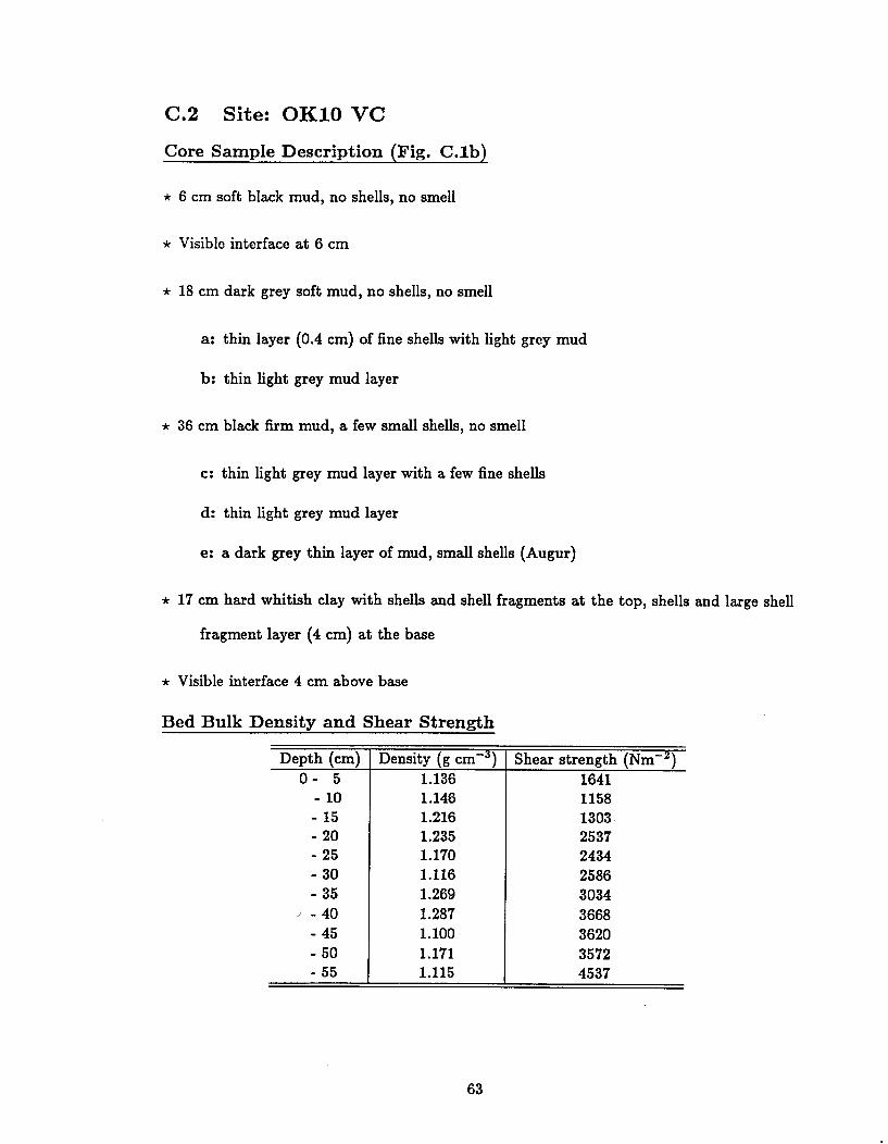
C.2 Site: OK10 VC

Core Sample Description (Fig. C.lb)

* 6 cm soft black mud, no shells, no smell

* Visible interface at 6 cm

* 18 cm dark grey soft mud, no shells, no smell

a: thin layer (0.4 cm) of fine shells with light grey mud

b: thin light grey mud layer

* 36 cm black firm mud, a few small shells, no smell

c: thin light grey mud layer with a few fine shells

d: thin light grey mud layer

e: a dark grey thin layer of mud, small shells (Augur)

* 17 cm hard whitish clay with shells and shell fragments at the top, shells and large shell

fragment layer (4 cm) at the base

* Visible interface 4 cm above base

Bed Bulk Density and Shear Strength

Depth (cm) Density (g cm - 3 ) Shear strength (Nm 2 )0- 5 1.136 1641

- 10 1.146 1158- 15 1.216 1303- 20 1.235 2537- 25 1.170 2434- 30 1.116 2586- 35 1.269 3034- 40 1.287 3668- 45 1.100 3620- 50 1.171 3572- 55 1.115 4537

63

C.3 Site: OK18 VC

Core Sample Description (Fig. C.lc)

* 4 cm black peat with a small amount of sand

* 2 cm light brown peat

a,b: 0.5 cm black peat

* 1.5 cm light brown peat

* 48 cm mottled firm peat with visible plant roots, no shell, no smell

40 cm mottled black and brown peat

8 cm mottled dark grey/light brown peat and sand

C.4 Site: OK31 VC

Core Sample Description (Fig. C.ld)

* 1 to 3 cm dark brown coarse sand, no shell

* Fine shells and fine shell fragments with sand

* 2 cm grey medium sand, no shell

* 1 cm dark grey sand layer

* 5 cm light grey coarse sand with fine or medium shells and small shell fragments

* 5 cm brown medium sand, no shell

* 18 cm sand layer, no shell, varying color from black at the top to mottled black and light

grey at the base, varying sand grain size from fine at the top to coarse at the base

64

APPENDIX D

SEDIMENT SAMPLING IN SPRING 1988

A field visit was undertaken in March 1, 1988 to obtain sample bottom cores using a

hand-held PVC piston corer designed at the Coastal Engineering Laboratory of the Univer-

sity of Florida, and to collect bottom sediment samples with a clamshell grab sampler for

sedimentary analysis. The ten sites visited are shown in Fig. D.1.

The cores were brought to the Coastal Engineering Laboratory where they were frozen

in a mixture of dry ice (frozen CO 2 ) and denatured alcohol, cut, and the bulk density of the

cut pieces were measured. Fig. D.2 shows a frozen, cut core from site 1. The mud/water

interface is fairly clearly defined by the observed color change. It should be pointed out that

the freezing procedure leads to an uneven expansion of the core longitudinally. However,

the procedure is fairly useful for examining the clarity of the low density region near the

mud/water interface.

In Table D.1 the total thickness of mud is given for different sites. The total mud thickness

was found to be generally consistent with what was obtained by Gleason and Stone (1975)

based on their mud thickness contours.

The fine-grained fractions of the collected mud samples were subjected to standard hy-

drometer test for size determination. A modification to the method was that the sediment

was not dried initially, since initial drying prevents complete dispersion of the sediment. In

order therefore to determine the total dry sediment mass required for calculation purposes,

the sediment was dried after the hydrometer test (Hwang, 1989).

The last four columns in Table D.1 give particle size characteristics (sizes d25 , dso and

d75, and sorting coefficient, So = (dis/d 2 5)1 / 2 ) for the fine-grained fractions at five sites.

Sediment samples at these sites were first separated into coarse and fine-grained fractions by

sieving through No. 200 Tyler sieve with an opening of 74 p m. It was found that between

about 75 and 90% of the material was fine-grained. This is generally consistent with the

observation of Gleason and Stone (1975) who found 93% of the mud by weight to be less

65

27- 101 427010'

81 * 0

#7

#2

#5

^ ~ *^ ...'" -' #

#5A

26045'| r80040 26045'

8004 0 '

O 5Km

Fig. D.1. Sediment/core sampling sites in Spring, 1988.

66

Mud/Water

Fig. D.2. Frozen core from site 1.

r 7

than 74 p m. They also found calcium carbonate to be present as a fine silt (2-5 pi m), and

quartz grains to be slightly larger.

The last column in Table D.1 gives loss on ignition (percent by weight) of the sediment

at various sites. The percent loss is fairly uniform, ranging from 36 to 41. This, in general,

is indicative of the high fraction of organic matter present in the sediment.

Table D.1: Bed and Sediment Characteristics

Site Total mud Fine particle characteristics IgnitionNo. thickness d2 5 dso d75 So loss

(cm) (p m) (p m) (p m) (%)1 30 c 15 10 2 2.7 402 36 24 15 1 4.1 363 _a 13 7 0.6 4.5 434 _ a 8 0.4 0.7 3.4 385 0 -a -a -a _a _a

5Ab 0 10 ~ 3 0.6 4.2 416 0 a _a _a _a _a

7 66 _a _a _a _a _ a

8 74 a_ _a _a _a _ a

9 33 a _a _a _a _ a

aNot measured.bAt this site the particle size analysis and ignition loss were obtained from a sample of

thin mud layer above hard bottom.CIncluding soft marl.

68

REPORT DOCUMENTATION PAGE FINE SEDIMENT REGIME...

Documents

Transcript of REPORT DOCUMENTATION PAGE FINE SEDIMENT REGIME...