Report: 2004-04-29 Development of a Test Method to Measure ...

Development of a Test Method to Measure Stationary and Portable Engine Emissions

Project Reference Number: CARB 00-06

Final Project Report April 29, 2004

Prepared for

California Air Resources Board P.O. Box 2815

Sacramento CA 95812

Submitted by:

Department of Mechanical and Aerospace Engineering P.O. Box 6106

West Virginia University Morgantown, West Virginia 26506

Federal or Entity Identification Number: 550665758

Mridul Gautam, Ph.D. (Principal Investigator) Professor

Voice: (304) 293-3111 ext. 2312 Fax: (304) 293-6689

Email: [email protected] Daniel K. Carder, Program Coordinator

Gregory J. Thompson, Assistant Professor Nigel N. Clark, Ph.D., Professor

Gurudutt Nayak, Graduate Research Assistant Mohan Krishnamurthy, Graduate Research Assistant

mailto:[email protected]

1 Disclaimer

The statements and conclusions in this Report are those of the contractor and not necessarily those of the California Air Resources Board. The mention of commercial products, their source, or their use in connection with material reported herein is not to be construed as actual or implied endorsement of such products.

ii

2 Acknowledgements

The researchers would like to thank Mid Atlantic Research Institute, LLC (MARI) for the free loan of the Real-time Particulate Mass Monitor, RPM100, for gravimetric particulate matter analysis. MARI also provided significant technical assistance, free of charge.

This Report was submitted in fulfillment of ARB Contract Number 00-06, “Development of a Test Method to Measure Stationary and Portable Engine Emissions” under the sponsorship of the California Air Resources Board. Work was completed as of December 29, 2003.

iii

3 Table of Contents

1 Disclaimer ....................................................................................................................... ii

6 Abstract........................................................................................................................ xxi 7 Executive Summary.................................................................................................. xxiii

2 Acknowledgements ....................................................................................................... iii 3 Table of Contents .......................................................................................................... iv 4 List of Figures................................................................................................................. x 5 List of Tables ............................................................................................................... xvi

7.1 Background.................................................................................................... xxiii

7.2 Methods.......................................................................................................... xxiv

7.2.1 Approach.................................................................................................xxiv

7.2.2 Test Engines ............................................................................................xxiv

7.2.3 Test Cycles ............................................................................................... xxv

7.2.4 Emissions Measurement Instrumentation................................................ xxv

7.3 Results............................................................................................................ xxvi

8 Nomenclature and Abbreviations............................................................................. xxx 9 Introduction.................................................................................................................... 2

9.1 Emissions Standards ........................................................................................... 5

9.2 Project Objectives ............................................................................................... 6

9.2.1 Original Project Objectives (Taken from the proposal) ............................. 7

9.2.2 Modified Project Objectives (December 2000) .......................................... 8

9.2.2.1 Specific Objectives ................................................................................. 9

9.2.3 Modified Work Plan (February 2003) ...................................................... 12

9.2.3.1 Lab Testing ........................................................................................... 12

9.2.3.1.1 Engines:........................................................................................... 12

9.2.3.1.2 Tests: ............................................................................................... 12

9.2.3.1.3 Fuel ................................................................................................. 13

9.2.3.2 Field Testing. ........................................................................................ 13

10 Previous Research...................................................................................................... 14 10.1 Summary of Literature Review......................................................................... 14

10.1.1 Recommendations from Task I Report (Literature Review and

Recommendations for Measuring In-use Emissions)................................................ 14

11 Experimental Equipment and Procedures .............................................................. 19 11.1 Introduction....................................................................................................... 19

iv

11.2 Approach........................................................................................................... 20

11.3 Test Engines...................................................................................................... 25

11.3.1 DDC Series 60 Engine:............................................................................. 25

11.3.2 Isuzu C240 ................................................................................................ 25

11.3.3 Caterpillar 3408........................................................................................ 27

11.3.4 Mack E7 .................................................................................................... 28

11.4 Test Cycles........................................................................................................ 30

11.5 Test Fuel............................................................................................................ 31

11.6 Candidate In-use Emissions Measurement Systems......................................... 31

11.6.1 Overview of MEMS................................................................................... 31

11.6.1.1 Flow Rate Measurement System ...................................................... 32

11.6.1.2 Gaseous Sampling and Sample Conditioning System...................... 33

11.6.1.2.1 Peltier Coolers............................................................................... 34

11.6.1.3 Engine Speed and Torque Measurement .......................................... 34

11.6.1.4 Data Acquisition, Reduction and Archival Subsystem..................... 35

11.6.1.5 Global Positioning Sensor................................................................. 35

11.6.1.6 Power Supply .................................................................................... 35

11.6.1.7 Transducers ....................................................................................... 35

11.6.1.7.1 Absolute Pressure Transducer....................................................... 36

11.6.1.7.2 Differential Pressure Transducer .................................................. 36

11.6.1.7.3 Relative Humidity Transducer...................................................... 37

11.6.1.8 Exhaust Gas Analyzers ..................................................................... 37

11.6.1.8.1 Carbon Dioxide Analyzer ............................................................. 38

11.6.1.8.1.1 General Features of BE-140 AD............................................ 38 11.6.1.8.1.2 Operating Principle of BE-140 AD........................................ 38

11.6.1.8.2 Oxides of Nitrogen Analyzer ........................................................ 39

11.6.1.8.2.1 General Features of MEXA 120 NOx .................................... 39 11.6.1.8.2.2 Operating Principle of MEXA 120 NOx................................ 40

11.6.1.8.3 General Features of Electrochemical NOx.................................... 41

11.6.1.8.3.1 Operating Principle of Electrochemical NOx......................... 42 11.6.1.9 Component Calibrations ................................................................... 42

11.6.2 Signal Model 3030PM Hydrocarbon Analyzer......................................... 43

11.6.3 Simple Portable On-vehicle Testing (SPOT) ............................................ 45

v

11.6.3.1 Introduction....................................................................................... 45

11.6.3.2 Exhaust Mass Flow rate Measurement ............................................. 47

11.6.4 Horiba OBS-1000 ..................................................................................... 48

11.6.5 Real-Time Particulate Monitor (RPM-100 QCM).................................... 49

11.7 Engine Dynamometer Laboratory..................................................................... 54

11.7.1 Dynamometer/Dynamometer Control....................................................... 54

11.7.1.1 Eddy-Current Dynamometers ........................................................... 54

11.7.1.2 Electric Dynamometers..................................................................... 54

11.7.2 Test Dynamometer Specifications............................................................. 54

11.7.2.1 Mustang Dynamometers PAU-100 (Isuzu C240)............................. 55

11.7.2.2 General Electric DYC-243 DC Dynamometer ................................. 55

11.8 Particulate Matter Sampling and Handling....................................................... 55

11.8.1 Dilution Tunnel ......................................................................................... 57

11.8.2 Critical Flow Venturi................................................................................ 58

11.8.3 Secondary Dilution Tunnel and Particulate Sampling ............................. 58

11.8.4 Gas Analysis System ................................................................................. 59

11.8.4.1 Hydrocarbon Analyzer...................................................................... 59

11.8.4.2 CO/CO2 Analyzer ............................................................................. 60

11.8.4.3 NOx Analyzer .................................................................................... 60

11.8.4.4 Bag Sampling.................................................................................... 60

11.8.5 Instrumentation Control and Data Acquisition ........................................ 60

11.9 Partial-flow Dilution Tunnel............................................................................. 61

11.10 Method 5 Analysis: ....................................................................................... 64

11.10.1 Principle and operation:....................................................................... 64

11.11 Modified Method 5 Test: .............................................................................. 66

11.12 DESIGN OF NOx CONVERTER................................................................. 68

11.12.1 Introduction........................................................................................... 68

11.12.2 Design of the NOx Converter ................................................................ 68

11.12.3 Need for a Converter Catalyst .............................................................. 69

11.12.4 Catalyst for the NOx converter.............................................................. 69

vi

11.12.5 Effect of the Sampling System Configuration on the Conversion

efficiency of the NOx Converter ................................................................................ 70

11.12.6 Inference on the Optimum Conditions for the NOx converter .............. 73

11.13 ON-ROAD ROUTES.................................................................................... 74

11.13.1 Saltwell, WV.......................................................................................... 74

11.13.2 Bruceton Mills, WV............................................................................... 75

11.13.3 Pittsburgh (Washington), PA................................................................ 76

12 Uncertainty Analysis.................................................................................................. 86 12.1 Introduction....................................................................................................... 86

12.2 Assumptions...................................................................................................... 86

12.3 Classification of Measurement Error ................................................................ 86

12.3.1 Random Error ........................................................................................... 86

12.3.2 Systematic Error ....................................................................................... 87

12.4 Classification of Components of Uncertainty................................................... 87

12.4.1 Uncertainty due to Random Error ............................................................ 87

12.4.2 Uncertainty due to Bias Error .................................................................. 87

12.5 Classification of Type of Uncertainty evaluation ............................................. 87

12.5.1 Type A Evaluation..................................................................................... 87

12.5.2 Type B Evaluation..................................................................................... 87

12.6 Measurement Uncertainty Sources ................................................................... 88

12.6.1 Calibration Uncertainty............................................................................ 88

12.6.2 Data Acquisition Uncertainty ................................................................... 88

12.6.3 Data Reduction Uncertainty ..................................................................... 88

12.6.4 Uncertainty due to Methods...................................................................... 88

12.7 Propagation of Uncertainty ............................................................................... 88

12.7.1 Absolute Summation.................................................................................. 89

12.7.2 Root-Sum of Squares Method.................................................................... 89

12.8 Uncertainty in Brake Specific Emissions ......................................................... 90

12.9 Calculating the Uncertainty of Concentration Values ...................................... 96

12.9.1 Calibration Error...................................................................................... 96

12.9.2 Data Reduction Error ............................................................................... 97

vii

12.9.3 Analyzer Error .......................................................................................... 97

12.9.4 Power or Energy Error............................................................................. 97

12.10 Results and Discussions on Uncertainty in Brake-Specific Emissions ...... 103

13 Results & Discussion: .............................................................................................. 104 13.1 Compliance Factor .......................................................................................... 104

13.2 Application of Compliance Factors for ISO 8178 Tests on an Isuzu C240 and a

DDC Series 60 Engine ................................................................................................ 111

13.2.1 Compliance Factor - Field Tests ............................................................ 119

13.2.2 Summary of In-Use Compliance Factor Approach ................................ 121

13.3 Qualification of MEMS .................................................................................. 122

13.3.1 Modal and Weighted Brake Specific NOx and CO2 Emissions for the Isuzu

C240 and DDC Series 60 Engines on ISO 8178 Tests ........................................... 122

13.4 Evaluation of MEMS with the WVU Heavy-duty Vehicle Emissions Testing

Transportable Laboratory............................................................................................ 126

13.5 Summary ......................................................................................................... 127

13.6 WVU Partial Flow-Dilution Tunnel : Determination of Total Particulate Matter

(TPM) 129

13.6.1 Summary ................................................................................................. 129

13.7 METHOD 5: Determination of Total Particulate Matter (TPM):.................. 131

13.7.1 Modified Method 5 Test:......................................................................... 133

13.7.1.1 Summary ......................................................................................... 136

13.8 AEI Simple Portable On-Vehicle Testing (SPOT) Testing ............................ 137

13.8.1 NOx Emissions......................................................................................... 138

13.8.2 Summary ................................................................................................. 140

13.9 Hydrocarbon Analyzer HFID Validation Testing........................................... 142

13.9.1 Response Test.......................................................................................... 143

13.9.2 Drift Test ................................................................................................. 144

13.9.3 Transient Tests: USFTP......................................................................... 147

13.9.4 Steady-State Test..................................................................................... 151

13.10 Horiba OBS-1000 ....................................................................................... 153

13.10.1 Summary ............................................................................................. 157

viii

13.11 COMPLIANCE FACTORS FOR ISO 8178 TESTS ON CATERPILLAR

3408 ENGINE............................................................................................................. 157

13.12 COMPLIANCE FACTORS FOR A MY1997 HEAVY-DUTY DIESEL

ENGINE FROM A CLASS 8 TRACTOR: FTP AND SIMULATED ON-ROAD

CYCLE TESTED ON AN ENGINE DYNAMOMETER.......................................... 158

13.12.1 Quantification of NTE Emissions based on NOx/CO2 Ratios ............. 158

13.13 In-field Testing............................................................................................ 160

14 Conclusions and Recommendations....................................................................... 168 14.1 In-use Emissions Compliance Recommendations .......................................... 169

14.2 In-use Emissions Measurement Tools (Portable and Stationary Engines) ..... 169

14.3 In-field Emissions Measurement Standard Operating Procedure................... 172

14.4 Recommendation of Future Research Activities ............................................ 174

15 References................................................................................................................. 177 Appendix A. Summary of Existing Regulations on Portable and Stationary

Appendix D. West Virginia University’s Quality Control/Quality Assurance Plan

Appendix F. ISO 8178 8-Mode Test for Isuzu C240 and DDC Series 60 Engine

Appendix G. Comparison of Mass Emissions Rates of NOx and CO2 Between MEMS and CVS Laboratory for ISO 8178 8-Mode Tests on DDC Series 60 and on

Engines 182 Appendix B. Review of Particulate Measurement Systems................................. 185 Appendix C. Literature Review ............................................................................. 194

240 Appendix E. Method 5 Theory and Analysis........................................................ 244

251

Isuzu C240 Engines....................................................................................................... 256 Appendix H. ISO 8178 Test Detail Results on Isuzu C240 and DDC Series 60. 260 Appendix I. Calibration Sheet for the Dry Gas Meter ....................................... 267 Appendix J. Procedure to Leak Check the Control Console of the Method 5 Sampling System ........................................................................................................... 268

ix

4 List of Figures

Figure 1 Isuzu C240 Mounted on a Custom Built Engine Test Stand with an Eddy

Current Dynamometer .............................................................................................. 27

Figure 4 Representation of the exhaust flow measurement system fitted to the test engine

Figure 12 Real-Time PM Mass Emissions Signal from CRT Equipped Engine As

Figure 13 Transient Real-Time PM Mass Emissions Signal from CRT Equipped Engine

Figure 14 of West Virginia University’s Engine and Emissions Research Laboratory

Figure 17 Lateral view of the Method 5 sampling system. Pitot tubes used for exhaust

Figure 19 Comparison of the NOx converter efficiency with a flow rate of 3.0 lpm at



Figure 2 Caterpillar 3408 Mounted on a DC Dynamometer Test Bed ............................. 28

Figure 3 Data acquisition and sampling conditioning and analysis systems of MEMS... 32

................................................................................................................................... 33

Figure 5 Schematic of the MEMS sampling system. [13] ................................................ 34

Figure 6 Schematic of the operating principle of the BE-140AD analyzer. ..................... 39

Figure 7 Schematic of the operating principle of NOx sensor .......................................... 41

Figure 8 Signal Model 3030PM portable hydrocarbon analyzer...................................... 44

Figure 9 Simple Portable On-vehicle Testing (SPOT) System ........................................ 46

Figure 10 AEI’s Proprietary Exhaust Flow Rate Measurement System........................... 48

Figure 11: Horiba OBS 1000 Series for in-use measurement,.......................................... 49

Measured by an RPM-100. ....................................................................................... 52

As Measured by an RPM-100................................................................................... 53

Emissions Measurement System............................................................................... 56

Figure 15 Schematic of the Partial-flow Dilution Tunnel (PM Cart) ............................... 63

Figure 16 Front view of the Method 5 sampling system .................................................. 65

flow rate measurement can be seen on the left. ........................................................ 65

Figure 18 WVU-MEMS NOx converter ........................................................................... 69

temperatures of 300° F, 325° F and 350° F using Horiba catalyst. .......................... 71

temperatures of 300° F, 325° F and 350° F using Horiba catalyst. .......................... 72

temperatures of 300° F, 325° F and 350° F using Vitreous Carbon catalyst. ........... 72

x


temperatures of 300° F, 325° F and 350° F using Vitreous Carbon catalyst. ........... 73

Figure 23 The Saltwell Route is indicated by the yellow highlighted section of the map.

The full route was a round-trip drive driven in two legs. The first leg was from

Figure 24 The Bruceton Mills Route is indicated by the yellow highlighted section of the

Figure 25 The Pittsburgh Route consisted of three legs, which are indicated with text

Figure 27 Time traces of vehicle speed, engine load, engine speed, bsCO2 and bsNOx




Figure 36 Comparison of MEMS Vs Lab NOx Mass Emission Rate over a WVU 5 Mile

Figure 37 Comparison of MEMS Vs Lab CO2 Mass Emission Rate over a WVU 5 Mile

Morgantown to the Saltwell Rd. exit and the second leg was the return trip. .......... 75

map. The full route was a round-trip drive driven in two legs. Morgantown to

Bruceton Mills was the first leg and Bruceton Mills to Morgantown was the second

leg.............................................................................................................................. 76

boxes. ........................................................................................................................ 77

Figure 26 Elevation Profile of the Sabraton to Bruceton Mills Route.............................. 79

during a SAB2BM route. .......................................................................................... 80

during a BM2SAB route. .......................................................................................... 82

Figure 29 Altitude profile for the SAB2SW route............................................................ 83

during SAB2SW route. ............................................................................................. 84

during SW2SAB route. ............................................................................................. 85

Figure 32 CO2 Mass Emission Rates For ISO 8178 Tests On Isuzu C 240 ................... 124

Figure 33 NOx Mass Emission Rates For ISO 8178 Tests On Isuzu C 240 ................... 124

Figure 34 CO2 Mass Emission Rates For ISO 8178 Tests On DDC Series 60 .............. 125

Figure 35 NOx Mass Emission Rates For ISO 8178 Tests On DDC Series 60 .............. 125

Transient Cycle ....................................................................................................... 128

Transient Cycle ....................................................................................................... 128

Figure 38 Comparison of Laboratory-Mini-tunnel BSPM Measurements ..................... 130

xi

Figure 39 Percentage Difference between Laboratory-Mini-tunnel BSPM Measurements

................................................................................................................................. 130

Figure 40 : A Multi-hole averaging nozzle on the left and a regular quartz “gooseneck”

nozzle on the right................................................................................................... 133

Figure 41 Comparison of Exhaust Flow Rates Measured by the SPOT and the MEMS on

an Idle Test.............................................................................................................. 138

Figure 42 NOx Concentrations Measured by the SPOT and the MEMS During an....... 139

On-road NOx Test ........................................................................................................... 139

Figure 43 NOx Concentrations Measured by the SPOT and the MEMS (MEXA 120 with

a ZrO2 Sensor, and an Electrochemical Cell) During an On-road NOx Test ......... 140


On-road NOx Test ........................................................................................................... 140

Figure 45 NOx Concentrations Measured by the SPOT and the MEMS During an...... 141

In-Laboratory Test .......................................................................................................... 141





Figure 48 Response Test using a Span Gas of 20 ppm Propane..................................... 143

Figure 49 A small scale time frame of the response test showing the response of the

instruments. ............................................................................................................. 144

Figure 50 Hydrocarbon comparison of the HFID for a zero air drift test, showing a scale

up to 10 ppm. .......................................................................................................... 145

Figure 51 Hydrocarbon comparison of the HFID for a zero air drift test....................... 145

Figure 52 Hydrocarbon comparison of the HFID for a span drift test............................ 146

................................................................................................................................. 146

Figure 53 Hydrocarbon comparison of the HFID for a span gas drift test, reduced scale.

Figure 54 Hydrocarbon comparison of the HFID for transient FTP test-1..................... 148

Figure 55 Hydrocarbon comparison of the HFID for transient FTP test-2..................... 148

Figure 56 A smaller time scale, an 150 second window, of the Hydrocarbon comparison

of the HFID analyzers for transient FTP test-1....................................................... 149

xii

Figure 57 Regression analysis of the HFID analyzers for transient FTP test-1.............. 150

Figure 63 Mass Emission Rates (g/s) of CO2 measured with the Horiba OBS-1000, WVU

Figure 64 Mass Emission Rates (g/s) of NOx measured with the Horiba OBS-1000, WVU

Figure 58 Regression analysis of the HFID analyzers for transient FTP test-2.............. 150

Figure 59 Hydrocarbon comparison of the HFID for steady state 6-mode test-1. ......... 151

Figure 60 Hydrocarbon comparison of the HFID for steady state 6-mode test-2. ......... 151

Figure 61 Regression analysis of the HFID for steady state 6-mode test-1.................... 152

Figure 62 Regression analysis of the HFID for steady state 6-mode test-2.................... 152

MEMS (MEXA 120) and Laboratory; Mack E7 Operated on the FTP.................. 154

MEMS (MEXA 120) and Laboratory; Mack E7 Operated on the FTP.................. 154

Figure 65 Mass Emission Rates (g/s) of CO2 measured with the Horiba OBS-1000, WVU

MEMS (MEXA 120) and Laboratory; Mack E7 Operated on a Simulated On-road

Route ....................................................................................................................... 155

Figure 66 Mass Emission Rates (g/s) of NOx measured with the Horiba OBS-1000, WVU

MEMS (MEXA 120) and Laboratory; Mack E7 Operated on a Simulated On-road

Route ....................................................................................................................... 155

Figure 67 Multiquip-Whisperwatt Diesel Powered AC Generator being tested for In-Use

Emissions ................................................................................................................ 161

Figure 68 Front view of the Generator. At the background is the transportable lab used

Figure 69 Comparison Of CO2 Mass Emission Rates From MEMS & Lab During In-Use

Figure 70 Comparison Of NOx Mass Emission Rates From MEMS & Lab During In-Use




for emissions measurement..................................................................................... 162

Operation Of The Generator. Run 1....................................................................... 163




Operation Of The Air Compressor. Run 1............................................................. 165

xiii





Figure 77 Comparison Of CO2 Mass Emission Rates From MEMS & Lab For a Section

Figure 78 Comparison Of NOx Mass Emission Rates From MEMS & Lab For a Section

Figure 79 SullAir 185 Diesel powered Air Compressor Being Tested For In-use

Appendix G 1 Figure G 1 Comparison of MEMS Vs Lab For ISO 8178 8 Mode Test On



Of The In-Use Test On The Air Compressor. Run 2 .............................................. 167

Of The In-Use Test On The Air Compressor. Run 2 ............................................. 167

Emissions ................................................................................................................ 168

Figure F 1 NOx Brake Specific Emissions For ISO 8178 Test On Isuzu C 240............. 251

Figure F 2 PM Brake Specific Emissions For ISO 8178 Test On Isuzu C 240.............. 251

Figure F 3 HC Brake Specific Emissions For ISO 8178 Test On Isuzu C 240 .............. 252

Figure F 4 CO Brake Specific Emissions For ISO 8178 Test On Isuzu C 240 .............. 252

Figure F 5 CO2 Brake Specific Emissions For ISO 8178 Test On Isuzu C 240............. 253

Figure F 6 NOx Brake Specific Emissions For ISO 8178 Test On DDC Series 60 ........ 253

Figure F 7 PM Brake Specific Emissions For ISO 8178 Test On DDC Series 60 ......... 254

Figure F 8 HC Brake Specific Emissions For ISO 8178 Test On DDC Series 60.......... 254

Figure F 9 CO Brake Specific Emissions For ISO 8178 Test On DDC Series 60.......... 255

Figure F 10 CO2 Brake Specific Emissions For ISO 8178 Test On DDC Series 60 ...... 255

Isuzu C 240 Run 1................................................................................................... 256

Figure G 2 Comparison of MEMS Vs Lab For ISO 8178 8 Mode Test On Isuzu C 240

Run 2 ....................................................................................................................... 256


Run 3 ....................................................................................................................... 257


Run 4 ....................................................................................................................... 257

xiv

Figure G 5 Comparison of MEMS Vs Lab For ISO 8178 8 Mode Test On DDC Series 60

Run.......................................................................................................................... 258


Run 2 ....................................................................................................................... 258


Run 3 ....................................................................................................................... 259

Figure I1: Calibration of the dry gas meter. The meter was calibrated using an 8 cfm

Laminar Flow Element from Meriam Instruments®. .............................................. 267

xv

5 List of Tables

Table 1 California Emissions Standards [5] ....................................................................... 6

Table 2 Federal standards set forth by the US EPA [5]...................................................... 6

Table 3 ISO 8178 Test Schedule For DDC Series 60 Engine .......................................... 24

Table 4 Engine Specifications (DDC Series60)................................................................ 25

Table 5 Engine Specifications (Isuzu C240) .................................................................... 26

Table 6 Engine Specifications (Cat 3408) ........................................................................ 28

Table 7 Specification of the Multiquip –Whisperwatt Diesel Powered Generator .......... 29

Table 8 Specification of the SullAir Air Compressor....................................................... 30

Table 9 ISO 8 Mode Test Cycle ....................................................................................... 31

Table 10 Absolute pressure transducer specifications. ..................................................... 36

Table 11 Differential pressure transducer specifications.................................................. 36

Table 12 Relative humidity transducer specifications ...................................................... 37

Table 13 Analyzers used................................................................................................... 37

Table 14 Specifications of MEXA 120 NOx analyzer ...................................................... 40

Table 15 Specifications of electrochemical NOx analyzer................................................ 42

Table 16: Test Matrix for the Additional Set of Method 5 Tests...................................... 67

Table 17 Catalysts used for the converter testing ............................................................. 70

Table 18 Sampling conditions for the NOx converter....................................................... 71

Table 19 List of instruments used for differential & absolute pressure and temperature

measurement ............................................................................................................. 93

Table 20 Errors in absolute pressure measurement .......................................................... 93

Table 21 Errors in differential pressure measurement ...................................................... 94

Table 22 Error in temperature measurement .................................................................... 94

Table 23 Specifications of instruments used in gaseous concentration measurement...... 96

Table 24 Specifications of gas analyzers used.................................................................. 97

Table 25 : Uncertainty Analysis for NOx , CO2 and PM Measurements On DDC Series

60. Run1.................................................................................................................... 99

Table 26 : Uncertainty Analysis for NOx , CO2 and PM Measurements On DDC Series

60. Run2.................................................................................................................... 99

xvi

Table 27: Uncertainty Analysis for NOx , CO2 and PM Measurements On DDC Series 60.

Run3.......................................................................................................................... 99

Table 28 : Uncertainty Analysis for NOx , CO2 and PM Measurements On Isuzu C 240.




Run1........................................................................................................................ 100

Run2........................................................................................................................ 100

Run3........................................................................................................................ 100

Run3........................................................................................................................ 101

Table 32 : Uncertainty Analysis for PM Measurements Using Method 5 System On Isuzu

C 240. ...................................................................................................................... 101

Table 33: Uncertainty Analysis for PM Measurements Using Method 5 System On DDC

Series 60.................................................................................................................. 102

Table 34 : Uncertainty Analysis for PM Measurements Using Mini-Dilution System On

DDC Series 60. ....................................................................................................... 102

Table 35 Application of the test method to generate compliance factors using In-field

pollutant ratio, I, from MEMS and Certification ratio C from the lab for Isuzu C 240.

Run 1. In-field Pollutant Ratio, I, is obtained using r2............................................ 112











pollutant ratio, I, from MEMS and Certification ratio C from the lab for DDC Series

60. Run 1. In-field Pollutant Ratio, I, is obtained using r2...................................... 114

xvii




























Table 49 In-use test results for 2001 Perkins engine. PM was collected for only two runs.

................................................................................................................................. 119

Table 50 In-use test results for 1990 Isuzu QD 100 engine. PM was collected for only

two runs................................................................................................................... 119

xviii

Table 51 Application of the test method on the 2001 Perkins engine. In field Pollutant

Ratio, I, obtained using r2........................................................................................ 119

Table 52 Application of the test method on the 1990 Isuzu QD 100 engine. In field

Table 53 Application of the test method on the 2001 Perkins engine. In field Pollutant

Table 54 Application of the test method on the 1990 Isuzu QD 100 engine. In field

Table 61 Comparison TPM collected with the Modified Method 5 at I50 Condition.

(Test#5 and #6 are Two Replicates that were conducted with ‘No-Preconditioned

Table 62 Comparison TPM collected with the Modified Method 5 at I75 Condition

(Test#11 and #12 are Two Replicates that were conducted with ‘No-Preconditioned

WVU MEMS, and Engine Laboratory over the Bruceton Mills Route Simulated on

Table 65 Application of the test method to generate compliance factors based on the

concentration values (F), and brake specific values (F’) of NOx and CO2 for ISO

Pollutant Ratio, I, obtained using r2. ....................................................................... 120

Ratio, I, is obtained using r1.................................................................................... 120

Pollutant Ratio, I, is obtained using r1. ................................................................... 121

Table 55 : Average Compliance Factor, F, values using CO2-specific information for

Isuzu C 240 and DDC Series 60 engines. ............................................................... 122

Table 56 : Average Compliance Factor, F, values using Fuel-specific information for

Isuzu c 240 and DDC Series 60 engines. ................................................................ 122

Table 57 ISO 8178 Test Results on Isuzu C240 (Run #1).............................................. 126

Table 58 ISO 8178 Test Results on DDC Series 60 (Run #1)........................................ 126

Table 59 Method 5 Results for two modes of the ISO 8178 tests on Isuzu C 240 ......... 132

Table 60 Method 5 Results for two modes of the ISO 8178 tests on DDC Series 60 ... 132

Filters’).................................................................................................................... 134

Filters’).................................................................................................................... 136

Table 63 Comparison of Brake-specific Emissions Measured with the Horiba OBS-1000,

WVU MEMS, and Engine Laboratory Over the FTP............................................. 156

Table 64 Comparison of Brake-specific Emissions Measured with the Horiba OBS-1000,

an Engine Dynamometer......................................................................................... 156

8178 test on Caterpillar 3408.................................................................................. 157

Table 66 Baseline NOx/CO2 calculations for a MY 1997 engine................................... 159

xix

Table 67 Specification of the Multiquip-Whisperwatt Generator .................................. 160

Table 68 Specification of the SullAir 185 Air Compressor............................................ 161

Table A 1 Existing Regulations for Stationary Engines ................................................. 182

Table A 2 Existing Regulations for Portable Engines ................................................... 183

Table A 3 Existing and Proposed Regulations for Diesel Fuel ...................................... 184

Table C 1 Gaseous Emissions Detection Methods ......................................................... 207

Table C 2 Available Portable Emissions Measurement Systems (Information was

provided by the manufacturers) .............................................................................. 215

................................................................................................................................. 223

Table C 3 Candidate Systems for Mass Measurement Investigated in the EMPA Study

Table H 1 ISO 8178 TEST RESULTS ON ISUZU C 240 RUN 1................................. 260








Table H 9 ISO 8178 TEST RESULTS ON DDC SERIES 60 RUN 1 ........................... 263

Table H 10 ISO 8178 TEST RESULTS ON DDC SERIES 60 RUN 1 ......................... 264





xx

6 Abstract

This study has developed test methods and protocols for determining compliance with emission standards for stationary and portable engines as promulgated by either the California Air Resources Board (CARB) or the U.S. Environmental Protection Agency (EPA). This study has resulted in a simple, cost-effective, yet accurate test method for stationary and portable engines to measure in-use emissions to ensure attainment of emission reduction goals. Additionally, the method will allow determination of compliance with the emission limits established by the Statewide Portable Equipment Registration Program. The method will allow measurement of fuel-specific emissions from both, diesel- and gasoline-fueled portable and stationary engines under real-world conditions. Given the fact that most stationary and portable engines are mechanically controlled engines, measurement of engine speed and load in the field would be not be a viable option, due to the associated complexity of such measurements. Hence, a “Compliance Factor” approach, based upon CO2-specific or fuel-specific emissions-measurements, has been developed and presented to CARB in this report. This method requires measurement of concentration of gaseous pollutants and the mass of particulate matter (PM) emissions. Errors introduced by the measurement of engine load and exhaust flow rate in determining brake-specific emissions are avoided. The Compliance Factor is a ratio of NOx and CO2 concentrations (In-field ratio, I) to the brake-specific mass emissions of NOx and CO2 (Certification ratio, C). The Certification ratio, C, is obtained either from the manufacturer, or from laboratory evaluation of the test engine on an ISO 8178 cycle. The test method presented to CARB was validated by running an extensive series of steady-state 8-mode tests (ISO 8178 cycle) that were conducted on both, mechanically and electronically controlled engines. It was also determined that the front-half of the Method 5 PM measurement methodology is in good agreement with the CVS system based engine certification PM test method. Further, a modified Method 5 sampling train comprising of a multi-hole sampling probe that spans the diameter of the exhaust stack, and a sample transfer tube maintained at ambient temperature could be a likely configuration for measuring PM from stationary and portable diesel engines in the filed. This approach does away with the cumbersome method of modifying the small diameter (2 inches to 6 inches for most applications) exhaust stacks of diesel engines, and traversing the exhaust stack to acquire samples at 8 locations along the stack diameter.

WVU has been involved with in-use, in-field measurements from heavy-duty vehicles for a decade using its transportable chassis dynamometer based emissions measurement laboratories. Today, evaluation of in-use, “real world” emissions from on-highway heavy-duty vehicles is gaining momentum due, in part, to the availability of transportable heavy-duty chassis dynamometer facilities developed by WVU, and the new in-use, on-board Mobile Emissions Measurement System (MEMS). Similar advances are essential for stationary and portable engines. However, it should be noted that measurement of in-use mass emission rates from on-highway vehicles is still an issue, and this is due to a lack of a “suitable” chassis test cycle that could be employed for all heavy duty vehicles (buses, trucks with automatic transmissions, as well as those with unsynchronized transmissions and low power-to-weight ratios). This problem of a lack of a single test cycle for the entire body of vehicles is dwarfed by the absence of any test cycle for “real world” testing of stationary and portable equipment and engines. Development of test

xxi

methods for in-use compliance of stationary and portable engines is now imperative in light of the urgent need to attain emission reduction goals, and develop inspection and maintenance (I/M) programs. The process of development and implementation of the test method presented to CARB for stationary and portable engines tapped into WVU’s experiences and “lessons learned” from the on-highway vehicle in-use emissions measurement exercises.

Recommendations have been made on the most suitable measurement tools for in-use emissions measurements, and Standard Operating Procedures (SOP) for conducting a in-field tests are also presented. WVU has recommended use of exhaust emission analyzers that can accurately and precisely measure gaseous concentrations, and a micro-dilution tunnel for filter-based gravimetric PM emissions measurements. This approach will reduce the cost of portable analyzer equipment by tens of thousands of dollars compared to the currently available commercial portable emissions measurement systems.

xxii

7 Executive Summary

7.1 Background

According to a recent EPA report [1], nonroad diesel engines are responsible for 44 % of total PM emissions and 12 % of total NOx emissions from all diesel sources nationwide. These numbers reflect the contribution of total nonroad diesel engines, which encompasses a vast array of applications, including equipment, vehicles and vessels, as well as stationary and portable diesel engines. It should be noted that throughout the literature nonroad and off-road terms are used quite interchangeably, encompassing the variety of applications referenced in the above-mentioned report. The report also notes that the particulate matter emissions from nonroad engines exceed those emitted by the on-highway engines, while emitting as much NOx as their on highway counterparts. Since 1996, emissions from these off-road engines are regulated and EPA aims at achieving over 60 % reduction in NOx emissions and over 40 % reduction in PM emissions from 1996 levels by the year 2007. Recent developments in exhaust gas after treatment promise 90% reduction in emissions, in conjunction with ultra low sulfur fuel usage. State and local governments, however, continue to regulate emissions from stationary and portable engines.

The objective of this study was to develop a cost-effective in-the-field test method for stationary and portable engines that would be used to determine compliance with emission standards for existing off-road engines. The proposed method and protocols will allow determination of compliance with emission limits established by the Statewide Portable Equipment Registration Program. The method will enable an accurate, cost-effective, and reliable measurement and quantification of fuel-specific mass emissions from both, diesel- and gasoline-fueled portable and stationary engines under real-world conditions. Fuel-specific emissions are defined as a ratio of mass of emitted pollutant per mass of fuel, or as a ratio of brake-specific emissions of the emitted pollutant per brake-specific emissions of carbon dioxide, assuming that the mass of hydrocarbons and carbon monoxide emissions in diesel engines is very small. A more thorough presentation of the equivalency of the fuel-specific and “CO2-specific” terminology is presented in Section 13.1. It should be noted that the mass of fuel can also be calculated as a product of the concentration of carbon dioxide and the molecular weight of fuel per carbon atom (12.01 + 1.008*(Atomic hydrogen to carbon ratio of the fuel)). Measurement tools discussed in this report could also be employed, if engine configurations allow, for determination of brake-specific emissions.

WVU believes that new in-the-field cost-effective test method for stationary and portable engines should be capable of determining compliance with emissions standards for newly manufactured off-road engines as promulgated by either the California Air Resources Board (CARB) or the U.S. Environmental Protection Agency (EPA). While several available, or soon-to-be-available, tools may be available for measuring brake-specific emissions in the field, it should be recognized that most of the stationary and portable engines are mechanically controlled, that is, they do not have any means of broadcasting engine speed and load. Hence, determining brake-specific emissions from these engines would be a daunting task, both from a cost and time perspective. Also, determination of

xxiii

mass emissions would involve measurement of exhaust flow rate, which is the largest source of uncertainty (as shown in a later section) in in-use emissions measurements. Moreover, limited access to exhaust stacks often makes measurements of exhaust flow rates practically infeasible.

7.2 Methods

Given all the constraints imposed upon in-use emissions measurements, WVU developed a method that uses concentration measurements only, and the equipment necessary to conduct such measurements is relatively inexpensive; hence, easily affordable. Compared to costs in excess of $100,000 of currently available on-board emissions measurement systems, the cost of equipment for the proposed method would be less than $10,000, and would require only one technician level individual to conduct the in-field test. Hence, each district could purchase several such units, and conduct large scale compliance testing.

7.2.1 Approach

WVU has developed, and validated a “Compliance Factor” based method for determining in-field compliance of stationary and portable engines. The Compliance Factor concept establishes a factor for the NOx/CO2 ratio that could be used to quantify in-field emissions. The Compliance Factor, F, is a ratio of the Infield pollutant ratio, I to the Certification ratio, C. The Infield pollutant ratio, I, can be obtained either as CO2-specific or as fuel- specific, that is, expressed as either mass of NOx per mass of CO2 or as mass of NOx per mass of fuel quantity. As shown later, the two Infield pollutant ratios, I, differ by a factor of 3.1717 (Equation 12-23). The Certification ratio, C, is a ratio of brake-specific emissions of NOx and CO2, and is obtained either from the manufacturer, or from laboratory evaluation on a ISO 8178 test cycle. The Certification ratio is brake-specific emissions based, since most certification data is available in this format.

The first step of the proposed method is to determine brake-specific emissions of CO2 and NOx, either from engine certification tests, or from manufacturer-supplied data. The ratio of the brake-specific emissions of NOx and CO2 will yield the Certification ratio, C. Concentration values of NOx and CO2, recorded during “in-use” emissions test are then utilized to determine the Infield pollutant ratio, I, either in terms of CO2-specific emissions or in terms of fuel-specific emissions. The ratio of the Infield pollutant ratio, I, to the Certification ratio, C, yields the Compliance factor, F = I/C, that could be used to determine compliance with emissions standards. It should be noted that WVU has made no attempt to establish a pass/fail criteria. Compliance Factor values are presented for various engines and tests, and these could be used by CARB as a guideline to determine a regulatory pass/fail criterion.

7.2.2 Test Engines

Tests were conducted on two different types of engines, namely, naturally aspirated, mechanically controlled engines, which would be typical of most stationary and portable engines, and turbocharged, electronically controlled engines, which are more characteristic of on-road applications. It should be noted that the on-road test engines

xxiv

merely served as a convenient test bed for evaluation of emissions measurement equipment. Although these evaluations were integral to the development of the test method, the intended nature of the engine application was not critical to the performance assessment of the candidate technologies. Listed below are the test engines that were used during this study:

A 1992 DDC Series 60 was tested while operating on a DC dynamometer testbed. The engine was an electronically controlled, turbocharged, 6 cylinder, 12.7 liters, inline configuration that was rated at 350 hp @ 1900rpm.

A 1997 Isuzu C240 was tested while operating on a eddy-current dynamometer test bed. The engine was a mechanically controlled, naturally aspirated, 4 cylinder, 2.4 liters, inline configuration that was rated at 56 hp @ 3000rpm.

A 1987 Caterpillar 3408 was tested while operating on a DC dynamometer testbed. The engine was a mechanically controlled, turbo-charged, 8-cylinder, 18 liters, V-8 configuration that was rated at 450hp @ 1900 rpm.

A 1989 WhisperWatt mode DCA-44SPXI generator, powered by a naturally aspirated 3.9L Isuzu QD-100 (4BD1) with a rating of 56 hp@1800 rpm, was tested in-field

A 2002 Sullair Model 1024-1932 portable air compressor, powered by a naturally aspirated 2001 Perkins 3.9L engine that was rated at 70 hp @ 2200 rpm, was also tested in-field.

7.2.3 Test Cycles

Qualification and validation of the proposed method comprised of extensive steady-state and transient tests that were conducted in the engine test cell, and also on a vehicle using the MEMS. Both batteries of tests included collection and analysis of concentration data, and brake-specific emissions data which included measurement of exhaust flow rates, concentrations, and engine speed and load as broadcast by the engine’s electronic control unit (ECU). Both engines were operated through the ISO 8178 8-mode steady state tests. For the in-field tests the portable equipment engines were tested as the units operated according to typical in-use duty-cycles. Although repeat tests were performed, test-to-test repeatability of the engine operating conditions were not critically investigated, since these were not devised test cycles, but normal in-use operation.

7.2.4 Emissions Measurement Instrumentation

Gaseous pollutants such as NOx, CO, CO2 and HC were measured using laboratory grade instruments. PM was measured gravimetrically using procedures outlined in CFR 40 part 89 subpart N [2]. PM in raw exhaust was measured using a Method 5 based apparatus while NOx and CO2 were measured using a portable emissions measurement system, MEMS (Mobile Emission Measurement System) developed by WVU. In addition, commercially available portable emissions measurement technologies like Analytic Engineering’s SPOT for NOx and CO2, Signal’s HFID based portable analyzer, Mid Atlantic Research Institute’s QCM-SCS for PM measurement and Horiba’s OBS 1000 on board emissions measurement instrument were evaluated at various stages of this study.

xxv

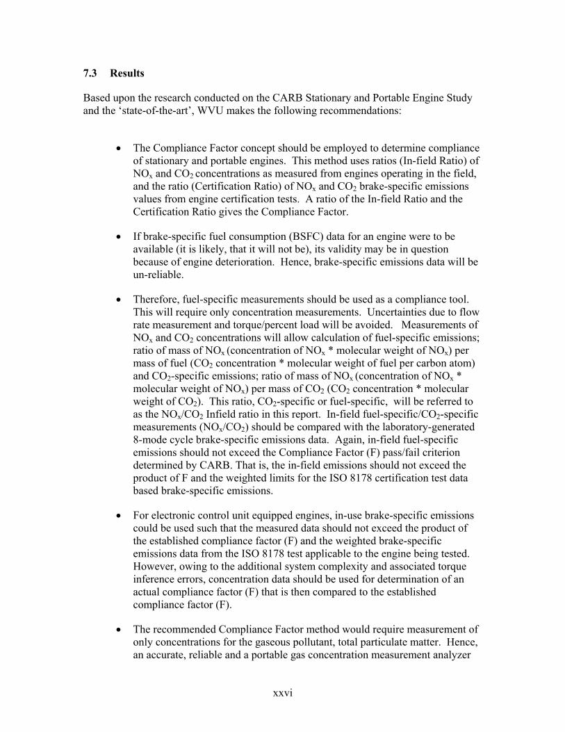
7.3 Results

Based upon the research conducted on the CARB Stationary and Portable Engine Study and the ‘state-of-the-art’, WVU makes the following recommendations:

• The Compliance Factor concept should be employed to determine compliance of stationary and portable engines. This method uses ratios (In-field Ratio) of NOx and CO2 concentrations as measured from engines operating in the field, and the ratio (Certification Ratio) of NOx and CO2 brake-specific emissions values from engine certification tests. A ratio of the In-field Ratio and the Certification Ratio gives the Compliance Factor.

• If brake-specific fuel consumption (BSFC) data for an engine were to be available (it is likely, that it will not be), its validity may be in question because of engine deterioration. Hence, brake-specific emissions data will be un-reliable.

• Therefore, fuel-specific measurements should be used as a compliance tool. This will require only concentration measurements. Uncertainties due to flow rate measurement and torque/percent load will be avoided. Measurements of NOx and CO2 concentrations will allow calculation of fuel-specific emissions; ratio of mass of NOx (concentration of NOx * molecular weight of NOx) per mass of fuel (CO2 concentration * molecular weight of fuel per carbon atom) and CO2-specific emissions; ratio of mass of NOx (concentration of NOx * molecular weight of NOx) per mass of CO2 (CO2 concentration * molecular weight of CO2). This ratio, CO2-specific or fuel-specific, will be referred to as the NOx/CO2 Infield ratio in this report. In-field fuel-specific/CO2-specific measurements (NOx/CO2) should be compared with the laboratory-generated 8-mode cycle brake-specific emissions data. Again, in-field fuel-specific emissions should not exceed the Compliance Factor (F) pass/fail criterion determined by CARB. That is, the in-field emissions should not exceed the product of F and the weighted limits for the ISO 8178 certification test data based brake-specific emissions.

• For electronic control unit equipped engines, in-use brake-specific emissions could be used such that the measured data should not exceed the product of the established compliance factor (F) and the weighted brake-specific emissions data from the ISO 8178 test applicable to the engine being tested. However, owing to the additional system complexity and associated torque inference errors, concentration data should be used for determination of an actual compliance factor (F) that is then compared to the established compliance factor (F).

• The recommended Compliance Factor method would require measurement of only concentrations for the gaseous pollutant, total particulate matter. Hence, an accurate, reliable and a portable gas concentration measurement analyzer

xxvi

would serve well. A filter-based gravimetric method using pre-conditioned and pre-weighed filter cassettes, and a micro-dilution tunnel is recommended for PM measurements. A modified Method 5 (with the front-half extraction) sampling train could be used, but the process could be avoided by using a micro-dilution tunnel because both procedures yield similar results. The modified Method 5 procedure would still require the extraction of the front half i.e. extraction of PM from the sampling probe and the front half of the filter holder plus the filter catch after every test. In addition, Method 5 procedure requires the use of glassware and a delicate, expensive quartz sampling probe. Using such a fragile set up for in-field testing for in-use PM measurements would require very competent handling, since such instruments are prone to breakage. Also, it is likely that many future off-road engines, including the portable & stationary engines, will implement the usage of exhaust after-treatment devices that may significantly change the speciation of PM downstream of the device. The disproportionate amount of soluble organic fraction (SOF) in relation to total particulate matter (on a mass basis) could result in poorer correlation of Method 5/Modified Method 5 with CVS dilution tunnel based methods. The use of micro dilution tunnel will result in condensation of these hydrocarbons on the filter and would also account for the atmospheric reactions of the particulate matter. This method, since it is mimicking the standard CVS dilution system, could likely provide for better comparison with the standard than the modified Method 5 procedure, which omits the dilution principle.

Equipment recommendations to conduct the proposed in-field test are as follows:

• PM Measurement

• Filter-based gravimetric PM measurement (using a portable mini-dilution tunnel, or even more compact micro-dilution tunnel(s))

• Modified Method 5 may be used, if essential. Modifications to the original Method 5 include, (i) multi-hole averaging sampling probe, (ii) ambient temperature probe, (iii) pre-conditioned and pre-weighed filters, and (iv) the front-half extraction should be included in the PM analysis

• Gaseous Emissions Concentrations

• NOx – Zirconium Oxide sensor with NO2-NO converter to measure NOx

• (NOx – Microflow NDIR soon to be available from Horiba; Non-dispersive ultra-violet analyzer from ABB)

• CO2/CO – Solid State NDIR

xxvii

• (CO2/CO – Ultra portable NDIR soon to be available through Horiba)

• HC – Portable HFID for diesel engines, possibly NDIR for spark ignited engines

• If non-sampling type sensors (those mounted directly in the exhaust stack) are not utilized, short heated sample line(s) and heated head pump(s) maintained at temperatures required by CFR 40, Part 89[2], and/or the ISO 8178 should be implemented to deliver exhaust samples to gaseous measurement devices.

• Power Supply

• Portable battery packs

• Data Acquisition

• 10Hz data collection (1 Hz would suffice for steady-state operation)

Authors believe that measurement of mass emissions is not necessary for determining compliance with the emissions standards. However, if mass emissions measurements are essential and desired, the authors’ recommendations are included below. It is noted that some components will be unchanged from those listed above, since concentrations of gaseous and PM emissions must be measured and integrated with additional measurements to arrive at mass emissions data.

• Exhaust Flowrate Measurements

• Annubar averaging pitot tube flowmeter

• (Portable ultra-sonic flow meter expected from Horiba)

• PM Measurement

• Filter-based gravimetric PM measurement (using a portable mini-dilution tunnel, such as the University of Darmstadt system)

• Modified Method 5 may be used, if essential. Modifications to the original Method 5 include, (i) multi-hole averaging sampling probe, (ii) ambient temperature probe, (iii) pre-conditioned and pre-weighed filters, and (iv) only the front-half extraction should be included in the PM analysis


xxviii


• (NOx – Microflow NDIR soon to be available from Horiba)




• If non-sampling type sensors (those mounted directly in the exhaust stack) are not utilized, short heated sample line(s) and heated head pump(s) maintained at temperatures required by CFR 40, Part 89[2], should be implemented to deliver exhaust samples to gaseous measurement devices.

Torque Measurement

• Inference from electronic control unit (ECU) data if available

• From the brake specific fuel consumption (BSFC) data, if available, for the engine. But, this data is always suspect because of engine and fueling system wear and tear, mal-maintenance, and possible engine re-builds since the original engine certification.

Electrical Power Supply

• Portable gasoline-powered generator if house power is unavailable

Data Acquisition


xxix

C

8 Nomenclature and Abbreviations

A Area at the Restriction β Diameter Ratio

Discharge Coefficient ∆P Difference in Pressure (P1 upstream – P2 restriction) gc Gravitational Constant k Specific Heat Ratio cp/cv

ρf Density of Flowing Fluid ρ0 Density of Fluid qm Mass Flow Rate r Ratio of P2 to P1 V0 Fluid Velocity Y Expansion Factor

A/F Air-to-Fuel Ratio ADC Analog-to-Digital Converter AIGER American Industry/Government Emissions Research BAR Bureau of Automotive Repair bhp Brake Horsepower BSFC Brake-Specific Fuel Consumption CFR Code of Federal Regulations CLA Chemiluminescent Analyzer CLD Chemiluminescent Detector CO Carbon Monoxide CO2 Carbon Dioxide DAC Digital-to-Analog Converter DOT United States Department of Transportation EAMP Emissions-Assisted Maintenance Procedure EC Electrochemical Cell ECat Electrocatalytic Cell ECM Electronic Control Module ECU Electronic Control Unit EMI Electro-Magnetic Interference EGS Electrochemical Gas Sensor EMA Emissions Measurement Apparatus FID Flame Ionization Detector FTIR Fourier Transform Infrared FTP Federal Test Procedures g Grams g/bhp-hr grams per brake horsepower-hour. GC Gas Chromatograph GPS Global Positioning System HC Hydrocarbon HFID Heated Flame Ionization Detector Hr Hour

xxx

I/M Inspection and Maintenance I/O Input/Output I.C. Internal Combustion (Engines) lpm Liters per Minute kB KiloByte kW KiloWatt MARI Mid-Atlantic Research Institute MEMS Mobile Emissions Measurement System MTU Michigan Technological University NDIR Non-Dispersive Infrared NDUV Non-Dispersive Ultraviolet NESCAUM Northeast States for Coordinated Air Use Management NIST National Institute of Standards Technology NMHC Non-Methane Hydrocarbons NO Nitrogen Monoxide NO2 Nitrogen Dioxide NOx Oxides of Nitrogen O2 Oxygen O3 Ozone OBD On-Board Diagnostic OS Operating System PC Personal Computer PM Particulate Matter ppm Parts Per Million PREVIEW Portable Real-Time Emission Vehicular Integrated Engineering

Workstation QCM Quartz Crystal Microbalance RF Radio Frequency ROVER Real Time On Road Vehicle Emissions Recorder SCS Sample Conditioning System (MARI Product) SO2 Sulfur Dioxide THC Total Hydrocarbons T90 Time required for response to exceed 90% of final value given a step

change input. T95 Time required for response to exceed 95% of final value given a step

change input. USB Universal Serial Bus U.S. EPA United States Environmental Protection Agency VOEM Vito’s On-the-Road Emission and Energy Measurement System VITO The Flemish Institute for Technological Research WCLA Wet Chemiluminescent Analyzer

xxxi

9 Introduction

Current inventories estimate that non-road engines contribute 20 percent of all nitrogen oxides (NOx) emissions and 50 percent of mobile source particulate (PM) emissions [3]. Construction equipment is estimated to contribute 12 percent of all NOx emissions. Emission inventories have grossly underestimated the emissions from mobile sources (on-highway and off-road), construction equipment, and portable and stationary engines. However, it should be noted that there is very limited in-field, in-use emissions data available from any of these emissions sources. While a significant level of effort is being focused on on-highway heavy-duty diesel engines, off-road equipment (portable, stationary and mobile) has been largely neglected. Limited off-road engines were subjected to emissions standards more than a decade after the on-highway emissions standards were promulgated. It is widely recognized that in-cell certification data is not representative of in-use, “real world” emissions from the same engines. Hence, comparisons between emissions data collected from in-field operations and laboratory testing can result in misleading conclusions. Moreover, emissions inventory models that rely solely upon certification data will most likely provide for unrealistic estimations of actual air inventories. California Air Resources Board (CARB) and the United States Environmental Protection Agency (USEPA) have recognized the need for widespread use of on-board emissions measurements. Recently the United States and the Settling Heavy-Duty Diesel Engine Manufacturers (S-HDDE) entered into “Consent Decrees” that requires a provision for emissions and compliance monitoring through in-use testing of engines. This compliance action demonstrated that mobile engine-powered equipment could be configured to emit low emissions under EPA test conditions (certification tests), yet under “real world” operating conditions, the equipment can emit 2 to 3 times EPA limits. The National Academy of Sciences recently indicated that more real-world data must be collected in order to more accurately predict the effects of the various emissions regulations. In light of recent developments in the emissions reduction programs, I/M programs, emissions compliance programs, and efforts to develop more realistic emission inventory models, the need for reliable emissions data from portable and stationary engines is highlighted by its absence.

Significant advances in combustion technology and reduction of fuel sulfur have resulted in reductions in gaseous and particulate matter emissions. The research team’s experiences in the US support the study by Ozturk et al. [8], in that maintenance practices of off-road equipment, as well as, on-highway equipment result in overfueling and combustion of higher amounts of lubricating oil. Emissions data collected by WVU from a 2-cylinder Lister Petter LPU-2 compressor engine, a John Deere 3049T road sweeper engine, and several other engines earmarked for a wide-variety of non-road applications (including stationary and portable engines) provide evidence that non-road engines do not produced the same levels of emissions as indicated by regulatory steady-state certifications cycles. Of course, there are instances when these engines are mal-maintained, and are very often over-fueled. This study is not aimed at investigating incidences of mal-maintenance.

WVU has recently completed Phases I, II and III of the “Consent Decree” work that required the selection, integration, qualification, correlation and use of portable

2

“suitcase” size emissions measurement equipment, Mobile Emissions Measurement System (MEMS), for use on heavy-duty vehicles. WVU also developed the test procedures and protocols for in-use, on-board emissions measurements from on-highway, heavy-duty vehicles. The Settling Heavy-duty Diesel Engine manufacturers (S-HDDE) have approved the use of WVU’s MEMS for compliance monitoring of their vehicles to fulfill the requirements of the “Consent Decree”. Unlike, commercially available portable emissions measurement systems, the MEMS has undergone major upgrades on a continuing basis. It has been WVU’s intent to continue modifying the MEMS, as sensor technology advances, and making the information available to regulatory and R&D organizations, instrument manufacturers, and engine industry. However, WVU is of the firm opinion that the portable emissions equipment technology is developing extremely rapidly, and now that the EPA and CARB have expressed a need for such equipment, we will see a phenomenal growth in the measurement accuracy, miniaturization of such instruments, and remote access via satellite links to emissions data on a real-time basis.

CARB defines a portable engine as an internal combustion engine which is designed and capable of being carried or moved from one location to another and does not remain at a single location for more than 12 consecutive months (This information may be obtained at http://www.arb.ca.gov/perp/perp.htm. Engines used to propel mobile equipment or a motor vehicle of any kind is not considered as a portable engine, and is not eligible for registration. A portable equipment unit is a portable piece of engine-driven equipment that is associated with, and driven solely by, a portable engine and emits pollutants over and above the emissions of the portable engine.

CARB has adopted a Portable Equipment Registration Program (PERP), which established a uniform program to regulate portable engines and portable engine-driven equipment units (Title 13, Chapter 9, Article 5, Sections 2450 – 2466 of the California Code of Regulations). Once registered in the PERP program, engines and equipment units can operate throughout the State of California without the need for individual permits to be issued by the local air districts. A summary of existing regulations regarding portable and stationary engines is given in Appendix A.

Portable engines include, but are not limited to, internal combustion (I.C.) engines used in the following:

• Cranes

• Pumps

• Welding

• Well Drilling

• Woodchippers

• Tactical support equipment

• Power generation

3

http://www.arb.ca.gov/perp/perp.htm

• Diesel pile-driving hammers

• Service or work-over rigs

• Dredges on boats or barges

• Compressors

Portable equipment units also include, but are not limited to, the following portable engine-associated units:

• Confined and unconfined abrasive blasting operations

• Concrete batch plants

• Sand and gravel screening, rock crushing and pavement crushing and recycling operations

• Tub grinders and trammel screens

• CARB lists specific requirements for portable engines. These requirements are dependent on whether the engine is classified as resident, non-resident, exempt, or meets State or federal non-road standards. Registered engines must comply with technological requirements which may include 4-degree injection timing retard, turbochargers, aftercooler/intercoolers, or catalysts.

In addition, some portable engines may be required to meet established emission limitations (shown in Table 1), visible emission limitations, fuel specification requirements, and recordkeeping and reporting requirements.

Portable equipment units registered in the Statewide Portable Equipment Registration Program are required to comply with established Best Available Control Technology (BACT) requirements. Additional registration requirements include: a daily emission limit of 82 pounds per day of particulate matter smaller than 10 microns, an annual limit of 10 tons per year for any criteria pollutant, and recordkeeping and reporting requirements.

Districts are pre-empted from permitting, registering, or further regulating portable engines and portable equipment units registered with PERP. However, local air districts are responsible for enforcing the Program. As a result, the air permit for a proposed project will require that the applicant maintain a current PERP registration for the generator sets used during construction phase that are 50 hp and greater, and that these generator sets must comply with the requirements of this program.

The design and development of a test method to determine in-use emissions for compliance with emission standards has to take place within the constraints of the State’s enforcement program. The local air districts have the primary enforcement responsibility. CARB or districts may conduct inspections at any time to verify and

4

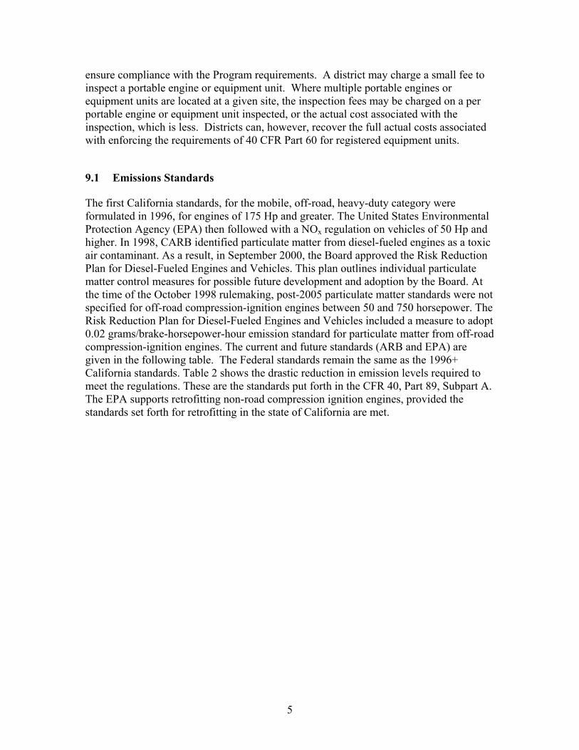
ensure compliance with the Program requirements. A district may charge a small fee to inspect a portable engine or equipment unit. Where multiple portable engines or equipment units are located at a given site, the inspection fees may be charged on a per portable engine or equipment unit inspected, or the actual cost associated with the inspection, which is less. Districts can, however, recover the full actual costs associated with enforcing the requirements of 40 CFR Part 60 for registered equipment units.

9.1 Emissions Standards

The first California standards, for the mobile, off-road, heavy-duty category were formulated in 1996, for engines of 175 Hp and greater. The United States Environmental Protection Agency (EPA) then followed with a NOx regulation on vehicles of 50 Hp and higher. In 1998, CARB identified particulate matter from diesel-fueled engines as a toxic air contaminant. As a result, in September 2000, the Board approved the Risk Reduction Plan for Diesel-Fueled Engines and Vehicles. This plan outlines individual particulate matter control measures for possible future development and adoption by the Board. At the time of the October 1998 rulemaking, post-2005 particulate matter standards were not specified for off-road compression-ignition engines between 50 and 750 horsepower. The Risk Reduction Plan for Diesel-Fueled Engines and Vehicles included a measure to adopt 0.02 grams/brake-horsepower-hour emission standard for particulate matter from off-road compression-ignition engines. The current and future standards (ARB and EPA) are given in the following table. The Federal standards remain the same as the 1996+ California standards. Table 2 shows the drastic reduction in emission levels required to meet the regulations. These are the standards put forth in the CFR 40, Part 89, Subpart A. The EPA supports retrofitting non-road compression ignition engines, provided the standards set forth for retrofitting in the state of California are met.

5

Table 1 California Emissions Standards [5]

California Emission Standards Reference for Non-road CI Engines

Rated Power Year CO

(g/bhp-hr)

HC (g/bhp-

hr)

NOx (g/bhp-

hr)

PM (g/bhp-

hr)

Class I (25 < hp) 1995-98 350 12.0 (HC + NOx) 0.9

1999+ 100 3.2 (HC + NOx) 0.25

Class II (25 < hp) 1995-98 350 10.0 (HC + NOx) 0.9

1999+ 100 3.2 (HC + NOx) 0.25

Class III (175≤hp≤750) 1996-2000 8.5 1.0 6.9 0.4

2001+ 2.6 1.0 5.8 0.16

Class IV (hp = 751+) 2000 8.5 1.0 5.8 0.16

Table 2 Federal standards set forth by the US EPA [5]

Rated Power (KW)

Tier Model Year CO

(g/bhp-hr)

HC (g/bhp-

hr)

NOx (g/bhp-

hr)

PM (g/bhp-

hr)

Tier 1 1996 11.4 1.3 9.2 0.54 25<KW<450 Tier 2 2001 3.5

0.2Tier 3 2006 3.5

In 1998, EPA adopted more stringent emissions standards for non-road diesel engines. Tier 3 of the standards addressed newer technologies for controlling PM. Major engine manufacturing companies have diligently pursued research and development of a wide variety of emission control technologies to meet the standards. These standards are expected to drastically reduce emissions from non-road diesel engines, which are already a major source of particulate matter and ozone-forming compounds. The US EPA and CARB have also taken steps towards curtailing in-use emissions concerns by developing newer standards to take effect in 2004 and even more stringent standards are to take effect in 2007.

9.2 Project Objectives

The original study objectives, as stated in the proposal, were modified as a result of consultations with ARB prior to commencement of work. Furthermore, based upon

6

findings, objectives and the test matrix were modified during the course of the project. Listed below are the original project objectives (as included in the project proposal) and the modified objectives, respectively.

9.2.1 Original Project Objectives (Taken from the proposal)

The objective of the proposed study was to develop a cost-effective in-the-field test method for stationary and portable engines that would be used to determine compliance with emission standards for existing manufactured off-road engines as promulgated by either the California Air Resources Board (CARB) or the U.S. Environmentally Protection Agency (EPA). The focus of this study will be on the development of a surrogate inspection-and-maintenance-type (I&M) test method for stationary and portable engines to measure in-use emissions to ensure attainment of emission reduction goals. The method will allow determination of compliance with emission limits established by the Statewide Portable Equipment Registration Program. The method will enable accurate, cost-effective, and reliable measurement and quantification of brake-specific mass emissions, as well as fuel-specific mass emissions from both, diesel- and gasoline-fueled portable and stationary engines under real-world conditions. Efforts will be directed towards identifying the effects of engine type and usage on mass emission rates.

Specific objectives of the study are:

1. To collect information on applicable test methods for stationary and portable engines, and to conduct an exhaustive literature search on the currently available technologies for monitoring in-use exhaust emissions, and their ability to consistently provide accurate, repeatable, and reliable mass emissions (brake specific in g/bhp-hr, and fuel specific g/kg of fuel) of gaseous (NOx, CO and HC) and particulate matter (PM10 in specific) under all operating and environmental test conditions. The candidate technologies will include on-board emissions measurement devices and certification/laboratory-grade analytical systems. Of particular interest would be the information on all the available methodologies for engine torque (or percent load) measurement. This effort will result in a report, to be submitted to CARB, on the available and potentially viable in-use emissions measurement systems for stationary sources, on-highway engines, and off-road engines. The cost of testing these engines will also addressed in the report.

2. To develop a test method using the information that was gathered in Task 1. The new method will allow emissions compliance testing of a wide range of engines operating in-the-field on different fuel types, using on-board instrumentation. The development and selection of the test method will be based upon WVU’s extensive experience in in-field measurements, and that of all the research and development groups (universities, R&D organizations, regulatory bodies, manufacturers, and instrumentation developers) that are involved in such activity. The development of the new method will closely scrutinize the need for correcting for potential errors in emissions

7

measurements using the same system for a wide range of engines.

3. To develop in-use testing protocols for stationary and portable engines. The protocols will include the total number of engines to be tested, criteria for test engine selection, a complete description of the test engines, and the proposed test schedule. It is proposed that development of these protocols be based upon laboratory evaluations of the selected test method (after CARB approvals) using laboratory grade equipment (such as, the equipment used for certification purposes). WVU is equipped with certification-quality test cells (recently underwent a very successful check by the U.S. EPA), transportable emissions laboratory with laboratory grade equipment and a total exhaust dilution tunnel (for PM measurements), and portable on-board emissions measurement instruments. WVU has also been promised access to the state-of-art emissions measurement instrumentation from leading manufacturers, namely, Horiba and Sensors, and R&D groups, such as, Mid-Atlantic Research Institute.

4. WVU has received both verbal and/or written commitments from industry and the EPA has also expressed a keen interest in providing WVU support if the work is approved. To achieve the fourth objective of the study, WVU will present to CARB the options of using WVU’s transportable emissions laboratory (with the instrumentation trailer and the portable eddy current engine test bed) and on-board emissions measurement instrumentation. Emissions measurements will be conducted under “real-world” conditions. Mass emission rates of particulate matter, oxides of nitrogen, carbon monoxide, total hydrocarbons and carbon dioxide will be determined. In addition, size selective particulate matter (PM10) measurements will be made both gravimetrically, and possibly, on a continuous, second-by-second basis.

The objectives, stated above, from the original proposal were modified in December 2000 based upon feed back from CARB. The modified objectives are listed below.

9.2.2 Modified Project Objectives (December 2000)

To develop a cost-effective in-the-field test method for stationary and portable engines that could be used as a screening tool to relate in-field emissions data with standards for newly manufactured off-road engines as promulgated by either the California Air Resources Board (CARB) or the U.S. Environmental Protection Agency (EPA). The focus of this study is to develop a surrogate inspection and maintenance (I/M) type test method for stationary and portable engines that will assist California in its mission of achieving attainment and continued compliance with federal and state ambient air quality standards.

The proposed study is focused on developing a viable, cost-effective, easy-to-use, and accurate in-field test method for stationary and portable engines that will yield in-use brake specific (or fuel specific) mass emissions data for NOx, PM, CO, HC, and CO2. The currently used steady-state ISO 8178 tests do provide a universally accepted method

8

of certifying these engines, but the mass emissions rates may not be representative of that particular equipment's usage. The in-field data could be compared to the ISO 8178 certification data from the engine manufacturer. It should be noted that WVU has measured brake-specific in-use emissions from small diesel-powered compressor engines, agricultural engines and off-road engines that have been considerably higher than the current applicable emission standards for such engines.

9.2.2.1 Specific Objectives

1. To collect information on applicable test methods for stationary and portable engines, and to conduct an exhaustive literature search on the currently available technologies for monitoring in-use exhaust emissions, and their ability to consistently provide accurate, repeatable, and reliable mass emissions (brake specific in g/bhp-hr, and fuel specific g/kg of fuel) of gaseous (NOx, CO and HC) and particulate matter (PM10 in specific) under all operating and environmental test conditions. The candidate technologies will include on-board emissions measurement devices and certification/laboratory-grade analytical systems. Of particular interest would be the information on all the available methodologies for engine torque (or percent load) measurement. This effort resulted in the Task 1 report, which was submitted to CARB, on the available and potentially viable in-use emissions measurement systems for stationary sources, on-highway engines, and off-road engines. The cost of testing these engines will also addressed in the report.

2. To develop a test method using the information that was gathered in Task 1. This will encompass design, development, and qualification of a portable emissions measurement system. The design and in-field application of this system will be dictated by the constraints as stated by this study. Details of the approach are discussed in the original proposal. Based upon WVU’s extensive experience in the area of mobile emissions measurement systems, it is anticipated that the system that will be designed for this study may include the following major sub-systems:

a. Exhaust mass flow measurement system b. Engine torque measurement (or inference) system c. Engine speed measurement system d. Exhaust gas sampling, and sample conditioning (depending

upon the level of accuracy desired) systems e. Data acquisition, reduction, and archival system

If the system is designed to measure fuel specific mass emissions, then the exhaust mass flow measurement system will be not be needed for gaseous emissions measurements. Simple concentration measurements will yield fuel specific gaseous emissions measurements. However, brake specific measurements of gaseous and PM emissions will require of mass flow measurement system. Engine torque from electronically controlled engines is

9

easily measured using a protocol adaptor. However, torque from mechanically controlled engines operating in the field may have to inferred using the CO2/engine speed method that WVU had developed for another CARB-funded off-road engines study. Concentrations of NOx emissions will be measured using a zirconia sensor, and CO2, CO and THC will be measured using a solid state NDIR. WVU is very familiar with the state-of-the-art in portable exhaust emissions measurement equipment. Concentration measurements of CO and HC will be a challenge with an NDIR. Carbon monoxide and total hydrocarbon concentrations in diesel engine exhaust are very low, and most of the portable analyzers do not yield accurate measurements at such low concentrations levels. Additionally, NDIR detectors do not respond very well to hydrocarbons other than alkanes (with negligible response even to methane). However, Sensors Inc. is currently working on an NDIR that can cover the entire range of hydrocarbons. Depending upon the level of sophistication required, the data acquisition could be a simple in-field data logger or an on-line, continuous data acquisition, reduction, and archival system. WVU has extensive experience with such systems.

The system development will involve extensive testing in the WVU engine and transportable laboratories. It is proposed that this study focus on three different types of applications, namely, generator sets, pumps, and compressors. Additionally, the system will be developed for various engine types (engine technologies), including naturally aspirated, turbocharged engines, mechanically controlled, and electronically controlled.

To achieve the objectives stated above, it is proposed that the system be first tested on two types of engines that will be representative of the engine technologies currently employed in the stationary and portable engines:

a. An Isuzu C240, naturally aspirated, mechanically controlled, six-cylinder, 145 cu. in. engine rated at 56 hp@3000 rpm

b. A MY1999, Cummins ISM, turbocharged, electronically controlled, six-cylinder, 10.9 liter engine rated at 370hp@1800 rpm.

Measurement of emissions from engines employed in different types of applications is discussed under items 3 and 4 of this document.

Testing the emissions on these two engines in the WVU engine test cells will not only allow us to compare the emissions measured by portable measurement system against laboratory grade measurement system, but also help to develop a method to compare emissions measurements on various basis (brake specific, fuel specific, etc.).

The engines will be tested on several steady state modes, on pseudo-transient cycles (emissions will be measured continuously while the engine is

10

operating through the steady state modes), and transient cycles (WVU). This allows us to collect emissions data under various modes of engine operation, and assess the limitations of the measurement system.

3. To further refine the test method on in-field engines using the WVU Transportable Laboratory’s emissions measurement system.

The problem of determining the accuracy and validity of in-field data will be established by measuring emissions from three in-field engines using the new test method, and comparing the data against the WVU Transportable Laboratory data.

It should be noted that WVU, per our proposal, had indicated our desire to meet with the CARB staff prior to selection of engines for emissions testing. We have maintained that selection of engines (of certain rating, given application, etc.) should be based upon the engine population and demographics in California. WVU intended to discuss these issues with the CARB staff prior to selecting the test engines.

It is proposed that the following engines available to this group be used to test the procedures on various engine applications:

a. Perkins 2.6 liter, naturally aspirated, mechanically controlled, 75 hp engine that is employed to drive blowers on the WVU Transportable Laboratory CVS. The engine will be tested while it is in use.

b. An Isuzu QD100, naturally aspirated, mechanically controlled, 3.8 liter engine, rated at 56 hp@1800 rpm.

c. A Cummins 5.9 liter engine, turbocharged, mechanically controlled engine rated at 135 hp@1800 rpm

4. Once the measurement system and the test method has been developed, it is proposed that 6 more engines, in various applications, be tested in the field. The WVU Physical Plant, Halliburton, and local mine equipment manufacturers, such as, Rohmac, Inc. will provide these test engines. The engines have not been specifically identified, but cooperative working agreements have been made that will enable WVU access to test these units. Available engines will range in size from approximately 50 hp to over 1000 hp. The current proposal did not identify any engines with power ratings exceeding 250 hp, but additional units with larger power ratings are available for testing. In-field engine tests involving engines of high power ratings should not necessarily impact the development of testing methodology, however, testing these engines tends to involve significantly more time and cost, particularly if the owner must be compensated for lost productivity or rental fees. Therefore, for the development of the in-field test methodology, the proposed equipment is the priority, while the additional six units will

11

serve, as a test option that could provide additional testing opportunities, should time permit.

9.2.3 Modified Work Plan (February 2003)

In February 2003, the test matrix was modified significantly after consultations with CARB. Inclusion of PM measurement per Method 5 protocols was the major addition to the workplan. WVU purchased the Method 5 sampling train using funds from sources other than CARB, and a significant amount of time was devoted to collecting valid Method 5 samples from diesel engine exhaust stacks. The following test matrix summarizes the changes that were effected on February 28, 2003.

9.2.3.1 Lab Testing

9.2.3.1.1 Engines:

Isuzu C-240 mining engine. The engine is a 4-cylinder, 4-stroke, mechanically controlled, naturally aspirated unit, with a rating of 57 hp @ 3000 rpm.

Mack E7-400 heavy-duty, on-highway engine. The engine is a 6-cylinder, 4-stroke, turbocharged unit, equipped with an electronic vehicle management and control system. The engine has a rating of 400 hp @ 1800 rpm.

WVU used a MY1992 DDC Series 60 heavy-duty, on-highway, 350 hp, electronically controlled, turbocharged, 6 cylinder, 12.7 liters, inline engine instead of the Mack E7. The DDC engine was available to this project for a longer period than the Mack E7. The additional time was needed to develop the Method 5 capability at WVU. The use of the DDC engine was approved by the CARB Program Manager,

9.2.3.1.2 Tests:

The Method 5 measurement procedure for total particulate matter (PM) will be employed for two steady state modes - R100 (rated speed – 100% load) and I75 (intermediate speed - 75% load) on the Isuzu C 240. Additional data from other modes will be collected if deemed necessary. The location of sampling section traverse points and the respective sampling duration times and sampling rates were consistent with procedures outlined in ARB Method 5 and Method 1A.

PM will also be concurrently measured using ISO-8178 gravimetric analysis (with the filter maintained at less than 125 F). Gaseous emissions including NOx, CO2, HC and CO will be measured using the WVU Mobile Emissions Measurement System (MEMS) and laboratory grade equipment operating according to procedures outlined in CFR 40 Part 86, Subpart N[8], and Part 89, Subpart E[2]. All measurement procedures would be in accordance with California emission test standards and test procedures for new 2000 and later off-road compression-ignition engines. These regulations are consistent with CFR 40, Part 89, Subpart E.

12

Engine work will be inferred from CO2 mass emissions rates and BSFC data, if available, for mechanically controlled engines, and from ECU data for electronically controlled engines.

9.2.3.1.3 Fuel

Ultra-low-sulfur fuel, i.e. less than 15-ppm sulfur, or standard on-highway diesel no. 2 fuel will be used for study.

Note:

Two repeats will be performed for each test set-point in order to establish repeatability.

Method 5 will be used for additional modes if required by CARB after reviewing results from the two modes.

A six cylinder, 4-stroke, mechanically controlled, naturally aspirated CAT 3306 may also be tested as part of the engine laboratory tests. The engine, currently being used by the Mining Safety and Health Administration, will be available upon request.

9.2.3.2 Field Testing.

A portable engine (Perkins 2.6 liter, naturally aspirated, mechanically controlled, 75 hp) that is employed to drive blowers on the WVU Transportable Laboratory CVS system will be tested while in use.

A stationary engine (yet-to-be-named, but WVU has received commitments from the WVU Physical Plant, Halliburton, and local mine equipment manufacturers, such as, Rohmac, Inc., to make such engines available for testing) ranging from 50 hp to 300 hp will be tested while in use.

Although the above engines were tentatively proposed as candidates for research, the research team later identified and tested alternative choices. A WhisperWatt mode DCA-44SPXI generator was used to operate a series of thermostatically controlled electric heating units, while emissions were concurrently measured using the WVU MEMS and the WVU Transportable Laboratory CVS system. This generator was powered by a naturally aspirated 3.9L Isuzu QD-100 (4BD1) with a rating of 56 hp@1800 rpm. A 2002 Sullair Model 1024-1932 portable air compressor was used to operate a jack-hammer, while emissions were concurrently measured using the WVU MEMS and the WVU Transportable Laboratory CVS system. The compressor was powered by a naturally aspirated 2001 Perkins 3.9L engine that was rated at 70 hp @ 2200 rpm.

Note:

As a result, Method 5 will be used for field-testing if required by CARB after reviewing results from lab testing.

1. Two repeats would be performed for each test to establish data repeatability.

13

10 Previous Research

A review of literature and recommendations for measuring in-use emissions were presented in the Task 1 report to CARB in early 2002 [7]. An updated, more thorough review is included in Appendix C. This appendix includes discussions of engine testing methods, portable emissions measurement equipment, and classification of emissions tests. A summary of the literature and recommendations for a measurement system for in-field testing of portable and stationary engines are presented below.

10.1 Summary of Literature Review

Portable exhaust emissions measurement systems offer a relatively inexpensive alternative to an emissions laboratory. While data collected with portable systems will likely be of lower quality than that collected in a laboratory with stationary, laboratory-grade equipment, it should be understood that the only way to conduct in-use emissions compliance testing of stationary and portable engines is with well designed portable exhaust emissions measurement systems. Furthermore, the test method developed in this study is independent of the innate uncertainties in measurements made with portable systems. The lower data quality is due, in part, to the limited analyzer technologies capable of operating under the relatively harsh conditions encountered in the in-field testing environment. The “Compliance Factor” concept developed by WVU employs only concentration measurements, which are the most accurate of all measurements made with portable emissions measurement systems. Although several manufacturers have systems designed to provide brake-specific mass emissions results, most of these systems are essentially prototypes. Very few of the complete systems have been sold and development work continues. To-date, WVU’s MEMS and the US EPA’s ROVER are the only two systems that have undergone extensive independent evaluations.

This study has reviewed the currently available methods for measuring emissions gas concentrations, particulate matter, exhaust flow rate, engine torque, engine speed, and ambient conditions. Also, data acquisition systems and factors affecting overall system operation were reviewed. This review is intended to provide information to allow an informed selection of an available portable emissions measurement system or selection of components to design a portable emissions measurement system for specific needs. Information comparing in-use emissions testing to stationary laboratory testing is also included for CARB’s consideration.

10.1.1 Recommendations from Task I Report (Literature Review and

Recommendations for Measuring In-use Emissions)

The following recommendations were made based on the literature search performed by WVU. Multiple recommendations were made where more than one device/method may be suitable. Recommendations that are shown in italics have been employed by WVU and proven to work well on on-highway vehicles.

14

• Exhaust Gas Flow Rate Measurement


• SF6 Tracer Gas with mass flow controller and NDIR detector

• V-Cone flowmeter, pending results of laboratory testing

• PM Measurement

• Tapered Element Oscillating Microbalance (TEOM)

• Filter-based gravimetric PM measurement (using a portable mini-dilution tunnel)

• Quartz Crystal Microbalance (gravimetric) to record real-time PM emissions

• Sample Conditioning System to provide desired dilution ratio


• NOx – Zirconium Oxide sensor with NO2 to NO converter to measure NOx

• CO2 – Solid State NDIR

• CO2/CO – Microflow NDIR


• Heated sample line(s), heated head pump maintained at temperatures required by CFR 40, Part 86

• Torque Measurement

• Inference from ECU data if available

• CO2 and engine speed matrices for mechanically injected diesel engines (This technique was developed for a CARB-funded off-road engine study)

• Electrical Power Supply


15

• Automatic switching device to switch from house power to generator power and vice-versa

• Battery back-up power supply for data acquisition computer and analyzers


• Laboratory-grade data acquisition system

• 10Hz data collection

• Datalogger

• In-use Emissions Limits Recommendations

• In-use brake-specific emissions should not exceed 1.5 times the weighted limits for the ISO 8178 test applicable to the engine being tested (This recommendation is in accordance with the efforts of CARB and EPA in the in-use emissions compliance arena)

• In addition to making in-field brake-specific emission measurements, it is recommended that fuel-specific emissions should also be recorded. It is very likely that an engine manufacturer may not be able to provide CARB with basic engine performance data, and that would be make brake-specific emissions calculations a difficult task. Under such circumstances, in-field fuel-specific measurements may be compared with the laboratory-generated 8-mode cycle fuel-specific emissions data. Again, in-field fuel-specific emissions should not exceed 1.5 times the weighted limits for the ISO 8178 test fuel-specific emissions results.

• In-field Emissions Measurement Standard Operating Procedure

• While it is understood that a Standard Operating Procedure (SOP) will be established in the next phase of the study, a sketch of a tentative SOP is presented below:

• Identify the test engine, and collect engine description (make, model, serial number, etc.) prior to site visit to “check-out” the engine.

• Ensure that the engine is in good working condition.

16

• Collect engine certification and performance data from the manufacturer.

• Transport portable gaseous and PM emissions measurement equipment, sample handling and conditioning systems, exhaust flow rate measurement systems, data acquisition, data archival and data analysis systems to the field.

• Prepare the engine for testing. That is, get access to the exhaust stack; for reasons of safety, request all non-essential (not conducting the test) to clear the area around the engine.

• Install flow meter on the engine exhaust stack.

• Install sampling probes and connect to the sample conditioning system/analyzers using heated lines.

• Connect data acquisition and control system (DAC) to the measurement systems.

• Power-up, warm-up and stabilize the concentration measurement analyzers, PM mass measurement systems, heated lines, DAC, etc.

• Leak-check the systems.

• Zero and span the analyzers

• Calibrate the analyzers.

• Warm-up the engine as follows:

o Idle (10 minutes, at least)

o Increase load in two increments and maintain the engine operating condition at each load for a period of 10 minutes, or until oil and coolant temperatures stabilize. It should be noted that most engines might not have temperature gages. Also, it should be noted that given the engine application, it might not be possible to increase the load on the engine. In such instances, the engine should be allowed to idle for 30 minutes. The actual warm-up procedure will be developed in the next phase of this study.

17

• Operate the engine over steady-state and transient modes of operation and collect emissions data (gaseous concentration, PM data, flow rates, engine speed, etc.). The actual engine operation will be dependent upon its intended application. The engine application may impose limitations upon how the engine may be run for emissions testing purposes.

o Emissions data, especially PM, should be collected for at least 20 minutes.

• Archive the data for off-site analysis.

• Dissemble emissions measurement equipment.

• Conduct final engine/equipment inspection to ensure that no damage was caused to the engine.

18

11 Experimental Equipment and Procedures

11.1 Introduction

This chapter discusses the equipment and procedures that were employed in this study. The chapter provides details of specifications of various sensors and analyzers that were incorporated into WVU’s Mobile Emissions Monitoring System (MEMS), AEI’s Simple Portable On-vehicle Testing (SPOT) system, Horiba’s OBS-1000 system, the total-exhaust double-dilution CVS system in the engine test cell at WVU’s Engine and Emissions Research Laboratory, Method 5 total particulate matter measurement system, the modified Method 5 system, WVU’s mini-dilution tunnel for sampling PM for gravimetric analysis and the portable Signal Model 3030PM heated flame ionization detector. This chapter also discusses the validation process of the suggested concept of a “Compliance Factor”, which uses the in-field NOx/CO2 concentration ratio and the corresponding brake-specific ratio from a certification test. This team of researchers believes that this cost-effective in-the-field test method for stationary and portable engines should be used to determine compliance with emissions standards. While several available or soon-to-be-available tools (such as those whose descriptions follow) may be available for measuring brake-specific emissions in the field, these systems are limited in that they rely upon ECU information to derive engine work output. It should be recognized that most of the stationary and portable engines are mechanically controlled, that is, they do not have any means of broadcasting engine speed and load. Hence, determining brake-specific emissions from these engines would be a daunting task, both from a cost and time perspective. Furthermore, determination of mass emissions would involve measurement of exhaust flow rate, which is the biggest source of uncertainty (as shown in a later section) in in-use emissions measurements. It is very likely that stationary and portable engines may not even offer in the exhaust stack to install the exhaust flowrate measurement sensors.

The design and development of an in-field test method for stationary and portable engines was constrained by the following:

• Mechanically controlled engines

• Inaccuracies in the ECU broadcast of engine load (in electronically controlled engines)

• Engine speed and torque measurements

• Exhaust flow rate measurements

• Size and weight of measurement system

• Ease of use and portability of measurement system

• In-field calibration of the test system

• Access for exhaust flow rate measurements on the target engine

19

• Fuel quality

• Set-up time for the measurement system

• Cost of the measurement system, and the total cost of conducting one in-field test (including personnel requirements)

• Qualifications of personnel conducting the in-field compliance testing

Given the above constraints, WVU developed a method that would use concentration measurements only, and the equipment necessary to conduct such measurements would be inexpensive; hence, easily affordable. These units could then be purchased in larger quantities by various districts interested in conducting compliance testing on stationary and portable engines.

Qualification and validation of the proposed method comprised of extensive tests that were conducted in the engine test cell, and also on an on-highway vehicle using the MEMS. Both battery of tests included collection and analysis of concentration data, and brake-specific emissions data which included measurement of exhaust flow rates, concentrations, and engine speed and load either measured on the engine dynamometer or as broadcast by the engine ECU.

11.2 Approach

In congruence with the objectives of this study, a method was developed that would provide for compliance criteria based upon fuel-specific/CO2-specific emissions measurements. The authors have developed a pollutant concentration-based test method in order to provide for a more compact, cost-effective approach, when compared to currently available test methodologies that would be based upon brake-specific mass emissions data. The resulting approach presented herein will provide an accurate, cost-effective, and reliable quantification of mass emissions from both diesel- and gasoline-fueled portable and stationary engines under real-world conditions.

WVU believes that a new in-the-field, cost-effective test method for stationary and portable engines should be capable of determining compliance for newly manufactured off-road engines, with specific standards and compliance details being promulgated by either the California Air Resources Board (CARB) or the U.S. Environmental Protection Agency (EPA). While several available or soon-to-be-available tools may be available for measuring brake-specific emissions in the field, it should be recognized that most of the stationary and portable engines are mechanically controlled, that is, they do not have any means of broadcasting engine speed and load. Hence, determining brake-specific emissions from these engines would be a daunting task, both from a cost and time perspective. Even determination of mass emissions would involve measurement of exhaust flow rate, which is the biggest source of uncertainty (as shown in chapter 12) in in-use emissions measurements, provided access is available on the engine stack to measure exhaust flow rate; hence qualification of mass emissions will be prone to errors.

The design and development of an in-field test method for stationary and portable engines were guided by consideration of the following factors:

20

• Mechanically controlled engines

• Engine speed and torque measurements

• Exhaust flow rate measurements

• Size and weight of the measurement system

• Ease of use and portability of the measurement system

• In-field calibration of the test system

• Access for exhaust flow rate measurements on the target engine

• Fuel quality

• Set-up time for the measurement system

• Cost of the measurement system, and the total cost of conducting one in-field test (including personnel requirements)

• Qualifications of personnel who will use the method.

Given the above constraints, WVU developed a method that uses concentration measurements only, and the equipment necessary to conduct such measurements could be very inexpensive; hence, easily affordable. Compared to costs in excess of $100,000 of currently available on-board emissions measurement systems, the cost of equipment for the proposed method would be less than $10,000, and would require only one technician level individual to conduct the in-field test. Hence, each district could purchase several such units, and conduct large scale compliance testing.

This chapter discusses the approach that was adopted for development of a viable test method. WVU has developed, and validated a “Compliance Factor” based method for determining in-field compliance of stationary and portable engines. The Compliance Factor concept establishes a factor for the NOx/CO2 ratio that could be used to quantify in-field emissions.

The first step of the proposed method is to determine brake-specific emissions of CO2 and NOx from either engine certification tests or from the manufacturer. The ratio of the brake-specific emissions of NOx and CO2 will yield the Certification ratio, C. Concentration values of NOx and CO2, recorded during “in-use” emissions test are then utilized to determine the Infield pollutant ratio, I, either in terms of CO2-specific emissions or in terms of fuel-specific emissions. The ratio of the Infield pollutant ratio, I, and the Certification ratio, C, yields the Compliance factor, F=I/C, that could be used to determine compliance with emissions standards. It should be noted that WVU has made no attempt to establish a pass/fail criteria. Compliance Factor values are presented for various engines and tests, and these could be used by CARB as a guideline to determine a regulatory pass/fail criterion.

21

Tests were conducted on two different types of engines, namely, a naturally aspirated, mechanically controlled engine, which is most representative of stationary and portable engines, and a turbocharged, electronically controlled engine.

Qualification and validation of the proposed method comprised of extensive tests that were conducted in the engine test cell, and also on a vehicle using the MEMS. Both battery of tests included collection and analysis of concentration data, and brake-specific emissions data which included measurement of exhaust flow rates, concentrations, and engine speed and load as broadcast by the engine ECU.

The approach adopted in this study is presented below:

• Conduct an extensive literature review of portable and laboratory-grade emissions measurement systems, which would allow measurement emissions concentrations, brake specific emissions, and fuel-specific emissions.

• Develop a set of preliminary recommendations on the equipment and protocols that should be used for in-field measurements.

• Acquire the following portable emissions measurement systems:

• AEI’s Simple Portable On-vehicle Testing system (with zirconium oxide sensor for NOx, solid state NDIR for CO2)

• Horiba’s OBS-100 (with solid state NDIR for CO2 & CO, zirconium oxide sensor, HFID for THC)

• Modify the WVU MEMS

• Any other available system for gaseous emissions measurement, such as Signal portable HFID.

• Modify the WVU mini-dilution tunnel for filter-based gravimetric analysis of PM, Method 5 PM measurement system and any other available system for PM emissions measurements.

• Acquire the following engines:

• A mechanically controlled, naturally aspirated diesel engine (Isuzu C240)

• An electronically controlled, turbocharged engine (DDC Series 60)

• A mechanically controlled, turbocharged engine (Caterpillar 3408)

• A Class-8 tractor (Mack) powered by a Mack E7 engine.

22

• Purchase a Method 5 PM sampling system, and make it operational. Adapt the sampling train for diesel exhaust stacks ranging from 2 inches in diameter to 6 inches in diameter.

• Qualify and validate the measurement tools, and methods in the WVU Engine and Emissions Research Laboratory’s engine test cells using steady-state test schedule, transient cycles, such as Federal Test Procedure (FTP) for heavy-duty engines, and cycles based upon in-field operation of heavy-duty vehicles. Compare results from the portable emissions instruments with the laboratory-grade analyzers and the CVS.

• Validate the measurement tools and the proposed approach on a Class-8 tractor over EPA approved test routes (approved on a study not related to this program) using WVU’s past experience in on-road emissions evaluation.

• Develop a set of data that includes Compliance Factors for various engines, and engine operations. These values could be used by CARB to propose a specific pass/fail criterion for in-use compliance testing.

• Modify the Method 5 PM measurement methodology in an attempt to develop a valid, yet simplified test for measuring PM in the field using the Method 5 sampling train.

• Develop a set of recommendations for CARB, which will comprise of:

• In-use emissions measurements – Parameters to be measured and instrumentation/sensors to accomplish the same

• In-use emissions compliance determination methodology

• In-field emissions measurement standard operating procedure

A Method 5 system was employed for gravimetric analysis of Particulate Matter (PM). Mobile Emissions Measurement System (MEMS) was used to measure mass emission rates of gaseous constituents like NOx and CO2 in raw exhaust. The data from the MEMS and Method 5 was compared with the laboratory grade analyzers and a correlation between the MEMS and the lab analyzers was established. All measurements were done in accordance with the requirements placed in CFR 40 part 89, subpart N. This correlation allowed the use of MEMS for in-use measurement purposes.

The MEMS was instrumented on a Class 8 Heavy Duty Mack truck to validate the test method. The truck was driven on different routes and an in-field ratio of NOx over CO2 for each route was developed. Since an On-highway engine was chosen for compliance testing, the in field ratios so obtained were compared against the FTP ratio. In addition to logging the emissions data, torque and speed data were also logged in from the ECU. The engine was then removed from the truck and was operated on the same on-road duty cycle through an engine dynamometer using the torque and speed data gathered from the

23

ECU. The engine was also exercised on the FTP certification cycle to collect the NOx over CO2 ratio information.

The in-laboratory tests on DDC Series 60 and Isuzu C 240 engines as well as the field tests on the Mack truck have led to the development of a set of compliance factors that give a better picture of conformance to emission standards during in use operation of the vehicle. Regulatory bodies, such as, CARB and EPA could utilize this information to develop criterion for in-use emissions compliance. With the added availability of the proposed test method, regulatory bodies should be able to better enforce their regulation and achieve their objective of attaining compliance to emission standards.

Table 3 ISO 8178 Test Schedule For DDC Series 60 Engine

ISO 8178 8-MODE STEADY-STATE CYCLE DDC Series 60

Mode Speed %Load

Weighting

Factor lbs-ft Rpm

1

Rated

100 0.15 1100

1800 2 75 0.15 841

3 50 0.15 561

4 10 0.1 112

5

Intermediate

100 0.1 1350

12006 75 0.1 1050

7 50 0.1 700

8 Idle 0 0.15 0 700

24

11.3 Test Engines

This study employed a naturally aspirated, mechanically controlled engine, typical of most stationary and portable engines in the field, and a turbocharged, electronically controlled engine for developing the test methods for in-field compliance purposes. These tests were conducted to study the amount of variation in the particulate matter emissions data measured using the partial-flow dilution tunnel and the QCM, and the gaseous emissions data measured using the MEMS compared to that measured using the full-flow dilution tunnel and the laboratory grade analyzers.

Given below are brief descriptions for each engine:

11.3.1 DDC Series 60 Engine:

An electronically controlled, turbo-charged, six-cylinder in-line Detroit Diesel Corporation Series 60 on-highway engine was used to generate exhaust for the validation tests. Table 4 lists the specifications of the engine.

Table 4 Engine Specifications (DDC Series60)

Engine Manufacturer Detroit Diesel

Corporation

Engine Model Series 60

Model Year 1992

Displacement 12.7 liters

Power Rating (hp) 360hp @ 1800 rpm

Configuration Inline-6

Bore (m) x Stroke (m) 0.13 m x 0.16 m

Induction Turbocharged

Fuel Type Diesel

Engine Strokes per Cycle Four

Injection Electronically Controlled

11.3.2 Isuzu C240

The Isuzu C240 is a pre-chamber, in-line four-cylinder, mechanically controlled engine that is used extensively in non-road applications, in general, and construction

25

application, in particular. This engine was critical in the development of test methods for mechanically controlled engine that do not allow measurement of engine speed and load without the installation and use of cumbersome and time-consuming instrumentation. Table 5 lists specifications for this engine.

Table 5 Engine Specifications (Isuzu C240)

Engine Manufacturer Isuzu

Engine Model C240

Model Year 1997

Displacement 2.4 liters

Power Rating (kW) 56hp @ 3000 rpm

Configuration Inline-4

Bore (m) x Stroke (m) 0.104 m x 0.12 m

Induction Naturally Aspirated

Fuel Type Diesel

Engine Strokes per Cycle Four

Injection Mechanically Controlled

26

Figure 1 Isuzu C240 Mounted on a Custom Built Engine Test Stand with an Eddy Current Dynamometer

11.3.3 Caterpillar 3408

The Caterpillar 3408 was an 18 liter, V-8 cylinder, mechanically controlled, direct-injection, turbo-charged, after-cooled engine is a parallel manifold design, with two intake and exhaust valves per cylinder. It has two full-flow oil filters and a fuel filter. The camshaft is in the center of the “v” with conventional valve lifters, push rods and rocker arms. This engine was being used in the WVU EERL by the PI in another study (funded by the South Coast Air Quality Management District) for another study that was investigating effectiveness of catalyzed traps in reducing emissions from non-road construction equipment. Tests were conducted on this engine to validate the “Compliance Factor” approach that is being presented to CARB for conducting compliance testing on stationary and portable engines.

27

Figure 2 Caterpillar 3408 Mounted on a DC Dynamometer Test Bed

Table 6 Engine Specifications (Cat 3408)

Engine Manufacturer Caterpillar 3408 DI

Engine Model No. 3408 DI

Engine Serial No. 48W24270

Model Year 1987

Rated Power 400 hp (299 KW) @ 1900 rpm

Peak Torque 375 lb-ft (1865 N-m) @ 1200 rpm

Bore 137.2mm (5.40 in.)

Stroke 152.4mm (6.00 in.)

Number and Arrangement of Cylinders V 8

Fuel/Air ratio 0.025

Firing Order (Injection Sequence) 1,8,4,3,6,5,7,2

11.3.4 Mack E7

Researchers employed a Mack CH613 over-the-road tractor, equipped with a 400 hp E7 engine and a Fuller 10 speed unsynchronized transmission, for on-road testing as well as

28

a second E7 engine, matched to the one in the vehicle, for engine dynamometer testing of Horiba OBS-1000 portable emissions measurement system. WVU operated the Mack tractor in conjunction with a tandem axle trailer that was loaded with concrete road barriers to vary the combination weight. Test weights used were approximately 60,000 lbs., confirmed with weigh tickets for all of the routes. These weights varied slightly during operation, due to fuel consumption and changes in vehicle occupants in the cab during testing.

Throughout operation on the routes, the truck was equipped with the MEMS to determine the engine speed and broadcast percent load from the electronic control unit (ECU) of the truck engine. The Mack tractor was equipped with a SAE J1587 interface; hence, engine load was broadcast by the ECU as a percent load signal. The translation of the “percent load,” broadcast by the engine, into a torque estimate is addressed elsewhere (Gautam et al., 2001). This process required knowledge of the engine lug down (full power) curve and the broadcast percent load under idle conditions throughout the engine speed range. The same methodology was used in the examination of routes to yield torque from the truck engine during operation. The outcome of the on-road study was a set of data that allowed comparison of ratios of brake-specific NOx emissions to the brake-specific CO2 emissions, and ratios of NOx concentrations to CO2 concentrations.

Table 7 Specification of the Multiquip –Whisperwatt Diesel Powered Generator

Multiquip-Whisperwatt Diesel Powered AC Generator

Model DCA-44SPXI

Generator Model DB-0667I

Phase Single

Frequency 60 Hz

Rated output 35 kW

Rated voltage 120 V 240 V

Rated current 182 A 182 A

Power factor 0.8

Engine Model 1990 Isuzu QD-100 (4BD1)

Type 4 cylinders, 4 stroke

Rated Output 56 hp @ 1800 rpm

Displacement 3853 cc

Fuel tank capacity 23.8 gallons

29

Table 8 Specification of the SullAir Air Compressor

SullAir 185 Diesel Powered Air Compressor

Model 2002 SullAir 185

Rated capacity and Pressure 185 CFM @ 100 PSIG (87L/s @ 7 Bar)

Maximum Pressure 125 PSIG @8.5 Bar

Rated Output 51.9 kW @ 2200 rpm

Engine Model 2001 Perkins

Type 4 Stroke 4 cylinders

Displacement 3.9L

Idle 800 RPM

Minimum Idle 1700 RPM

11.4 Test Cycles

Most of the test method development was conducted on different engines in the Engine and Emissions Research Laboratory Test Cells at WVU. The on-road testing of a Class 8 Tractor with WVU MEMS was conducted to validate the proposed “Compliance Factor” concept.

The primary cycle used throughout the course of this program was the ISO 8178 Type C1 8-mode Steady State Cycle for Off-road Vehicles, and Diesel Powered Off-road Industrial Equipment (see Table 10). This program comprised of raw exhaust testing for gaseous emissions using the WVU MEMS and other portable emissions measurements systems, and simultaneous dilute exhaust measurements using laboratory-grade analyzers and CVS; PM measurements using the CVS based method, partial flow dilution tunnel (mini-dilution tunnel), Method 5 and a modified Method 5; evaluations of various portable analyzers and sensors; testing over simulated on-road “real-world” operation of heavy-duty tractors, and the heavy-duty FTP cycle; and MEMS evaluation on the WVU Transportable Laboratory. Hence, the ISO 8178 8-mode cycle was not employed in its entirety for all tests. Details of actual test cycles and test modes are presented in this chapter under specific tasks.

30

Table 9 ISO 8 Mode Test Cycle

ISO 8178

Mode Number

Engine Speed Observed Torque

( Percentage of max.)

Modes Selected

for Testing 1 Rated 100 √

2 Rated 75 √

3 Rated 50 √

4 Rated 10 √

5 Intermediate 100 √



8 Idle 0 √

11.5 Test Fuel

Federal diesel no. 2 was used for all in-lab and in-field testing. Since this study was focused on development of a test method, a decision was made in consultations with the Program Manager that Federal Diesel No. 2 would suffice. The fuel was characterized by a Cetane number of at least 40, and a maximum aromatic content of 35.

11.6 Candidate In-use Emissions Measurement Systems

At the onset of the study WVU identified a number of candidate emissions measurement systems that were available for adaptation to in-field emissions testing of portable and stationary engines. Most of these systems have been developed for on-board testing of on-highway vehicles, however, the requirements of an emissions measurement systems for portable and stationary engines do not differ significantly from those of on-board systems. Included below are the results of evaluation testing conducted on various portable emissions measurement systems. It should be noted that some of these evaluations were performed using engines configured for uses other than portable and stationary vocation, however, for system evaluation purposes this would not affect conclusions drawn concerning test methodology.

11.6.1 Overview of MEMS

The following sections discuss the various components of the MEMS system and their operation. Figure 3 shows the data acquisition and flow conditioning and analysis systems of MEMS.

31

Also discussed are the calibration procedures that were followed for the various transducers, sensors and the analyzers during the testing program. The major components of the MEMS system are the emissions sample conditioning and analysis box; exhaust flow rate measurement system and the data acquisition system

Figure 3 Data acquisition and sampling conditioning and analysis systems of MEMS.

11.6.1.1 Flow Rate Measurement System

Exhaust mass flow rates were measured with a Dietrich Standard AnnubarTM [Figure 4]. The Annubar is a multi-point averaging pitot tube that works on the principle of Bernoulli’s theorem. Of the different configurations of the AnnubarTM, the regular threaded Pak-Lok assembly (Model DCR+15S or Model DCR+25S) was used for the measurement process. Flow rate calculations required accurate measurements of differential and absolute pressures, and the exhaust gas temperature. Transducers that were used for the purposes are listed in detail later in this section. Figure 4 gives a representation of how the flow measurement system was fitted on the engine.

32

Transducer Box

Annubar

Heated Line

Exhaust Stack

Figure 4 Representation of the exhaust flow measurement system fitted to the test engine

11.6.1.2 Gaseous Sampling and Sample Conditioning System

The sampling probe that was placed in the exhaust stream complies with the regulations set by the 40 CFR, Part 89.412.96. The stainless probe, which has nine ports along its periphery, was placed spanwise across the flow so that representative sample is drawn from the exhaust stream. The other components of the exhaust sampling system included: heated Teflon line, heated filter and the pump. The heated Teflon sample line 0.25” outer diameter was used to transfer the sample from the sample probe to the heated filter. Heating the sample prior to any drying device prevents condensation. The MEXA 120 Zirconium Oxide NOx sensor was placed downstream of the heated filter and upstream of the Air Dimensions Inc. Micro Dia-Vac sample pump. A NO2 to NO converter was incorporated with the NOx sensor manifold to minimize space requirements.

A proprietary NOx converter was designed and tested to allow for accurate measurements of NOx emissions. It should be noted that engines without exhaust aftertreatment systems emit NO2 emissons that constitute 3% - 10% of total engine out NOx. However, use of catalyzed traps to control PM emissions could result in NO2 emissions that will constitute nearly 30%-35% of total NOx. Hence, it is imperative that an effective, unlike commercially available NO2 to NO converters, be designed and used for in-field raw exhaust emissions measurements. Details of the NO2 to NOx converter are presented later in this chapter.

33

https://89.412.96

Hubi:dLin:! lnp,it

Hut,d Filter

Zi02NO Seruor

NO2 - NO Converter

Diaph,,gm !,,imp

Come2\$ate Drain

Pressure Regulator

Differential

Logenl for S amp!, - Heated

---Non-Hu t,d

Hom>• EE-140 CO2/CO NDIR

Araly-,,,r

flow Meter

ElectJOchemic&! Control V &Iv,

j

Electro:hemical NO Cell

Exlw.i,t

Downstream of the pump, a custom-designed compact Peltier effect gas chiller removed moisture from the sample stream, and provided an outlet dew point of approximately 40°F. A differential pressure regulator, in conjunction with needle valves, controlled flow rate to the CO2 analyzer and the electrochemical NO sensor to 3.0 LPM and 0.5 LPM respectively. A schematic of the sampling system is shown in Figure 5.

Figure 5 Schematic of the MEMS sampling system. [13]

11.6.1.2.1 Peltier Coolers

Humidity in the exhaust sample was removed in order to quantify the emissions measurements as “dry” measurements. This was achieved by chilling the sample to lower the dew point temperature, and then condensing the moisture in the sample. The gas chiller consisted of a thermo-electric chiller (TEC), which is solid-state heat pump that employs the Peltier effect. During operation, DC current flows through the TEC causing heat to be transferred from one side of the TEC to the other, creating a cold and hot side. The thermal energy is transferred from the hot side to a heat sink, which dissipates the heat to the environment. This dissipation of thermal energy present in the sample helps in lowering the dew point temperature and aids in the condensation.

11.6.1.3 Engine Speed and Torque Measurement

The ECU broadcast was used to record the various engine and vehicle parameters including, engine speed and also vehicle speed. The vehicle speed broadcasted can be used to infer the distance traveled, which was determined with the GPS in the MEMS. The ECU also broadcasts engine load on a percent basis. The engine speed is generally broadcast at 10 Hz with a resolution of 0.25-rpm resolution and the engine percent load at

34

10 Hz with a 0.5% resolution. The broadcast ECU load was derived from fuel consumption, and that was inferred from fuel injector flow rate information. Therefore, ECU engine load is a prediction of total work performed by burning a given quantity of fuel. The ECU load estimation included frictional loads inherent to the mechanical assembly and accessory loads, which had a negative effect in terms of actual work available for use by the vehicle. In some cases the ECU load estimates exceeded 100%, but that was that is largely due to the manufacturer’s desire to utilize all of the system resolution.

11.6.1.4 Data Acquisition, Reduction and Archival Subsystem

The data acquisition system (DAS) used by MEMS was designed to withstand the vibrations encountered during on-road testing. The DAS was so configured that it can adapt to a wide array of test vehicles and variety of signals.

The DAS was controlled by an Advantech PCM-9570/S single board computer (SBC) running at 850 MHz and supported by a 256 MB RAM. The SBS was configured with PC104 capabilities, which allowed the system to be more modular, and reduced the overall size of the system. The signal conditioning of analog signals were done using a SC-2345 National Instruments signal conditioning system. A National Instruments PCMCIA E-Series DAQ Card-6062 read the conditioned signals. The DAQ card can have up to 16 analog input channels and 12 bits resolution. The ECU broadcast information was communicated to the SBC through the use of a Dearborn Group (DG) DPAIII/PC104 Protocol adapter. For some test vehicles, the ECU interface was also alternatively provided by means of a DPA II or DPAIII Serial Port Protocol adapter. These components were integrated and installed into a custom-fabricated aluminum enclosure. The enclosure also housed the control panel for the Horiba MEXA 120, as well as the keyboard, mouse, and the front panel LCD monitor.

11.6.1.5 Global Positioning Sensor

The GPS is not required for stationary and portable engine applications. However, it was incorporated into the MEMS to provide a redundant method for measuring vehicle speed along with the broadcasted ECU speed for on-highway applications. A Garmin GPS35 was mounted on each vehicle as part of the MEMS equipments.

11.6.1.6 Power Supply

The vehicle-mounted generator set will fulfill the power requirements of the current MEMS design. Surge protectors are used for the DAS.

11.6.1.7 Transducers

Various transducers were used as part of flow measurement system of MEMS. It includes transducers for the measurement of pressure, differential pressure, temperature and relative humidity.

35

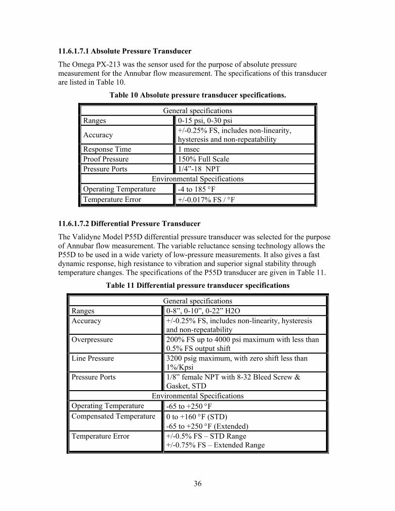
11.6.1.7.1 Absolute Pressure Transducer

The Omega PX-213 was the sensor used for the purpose of absolute pressure measurement for the Annubar flow measurement. The specifications of this transducer are listed in Table 10.

Table 10 Absolute pressure transducer specifications.

General specifications Ranges 0-15 psi, 0-30 psi

Accuracy +/-0.25% FS, includes non-linearity, hysteresis and non-repeatability

Response Time 1 msec Proof Pressure 150% Full Scale Pressure Ports 1/4”-18 NPT

Environmental Specifications Operating Temperature -4 to 185 °F Temperature Error +/-0.017% FS / °F

11.6.1.7.2 Differential Pressure Transducer

The Validyne Model P55D differential pressure transducer was selected for the purpose of Annubar flow measurement. The variable reluctance sensing technology allows the P55D to be used in a wide variety of low-pressure measurements. It also gives a fast dynamic response, high resistance to vibration and superior signal stability through temperature changes. The specifications of the P55D transducer are given in Table 11.

Table 11 Differential pressure transducer specifications

General specifications Ranges 0-8”, 0-10”, 0-22” H2O Accuracy +/-0.25% FS, includes non-linearity, hysteresis

and non-repeatability Overpressure 200% FS up to 4000 psi maximum with less than

0.5% FS output shift Line Pressure 3200 psig maximum, with zero shift less than

1%/Kpsi Pressure Ports 1/8” female NPT with 8-32 Bleed Screw &

Gasket, STD Environmental Specifications

Operating Temperature -65 to +250 °F Compensated Temperature 0 to +160 °F (STD)

-65 to +250 °F (Extended) Temperature Error +/-0.5% FS – STD Range

+/-0.75% FS – Extended Range

36

11.6.1.7.3 Relative Humidity Transducer

The Omega model HX92-A was used for the purpose of monitoring continuous ambient relative humidity and temperature. A thin-film polymer capacitor senses relative humidity. The transmitter output is linearized and temperature compensated. A stainless steel mesh-wire filter that is easily removable for cleaning protects the sensor. The specifications of this transducer are provided in Table 12.

Table 12 Relative humidity transducer specifications

Input Voltage Range 24 Vdc Measuring Range 3 to 95% Temperature -4 to 167 °F

Accuracy +/- 2.5% RH from 20 to 80% RH +/- 3.1% RH below 20 and above 80% RH

Output Voltage 0 to 1Vdc for 0 to 100% RH RH Temperature Compensation -4 to 167 °F RH Time Constant (90% response at 25° C, in moving air at 1m/s)

>10 seconds, 10 to 90% RH

>15 seconds, 90 to 10% RH

Repeatability +/-1% RH, 0.5 °F

11.6.1.8 Exhaust Gas Analyzers

Oxides of nitrogen (NOx) and carbon dioxide were identified as the key gaseous pollutants to be measured. Table 13 gives the list of analyzers used, their operation type, the detection device used and their source.

Table 13 Analyzers used

Source Horiba

Instruments, Inc.

Horiba

Instruments, Inc. Sensors Inc.

Model BE-140 AD MEXA-120 AMB-II

Operation Type NDIR Zirconium oxide

(ZrO2) Electrochemical

Detection Device Solid State Optical Non-Sampling

ZrO2 Solid State optical

Gases Measured CO2 NOx NO

37

11.6.1.8.1 Carbon Dioxide Analyzer

The BE-140 AD five gas analyzer was used for the measurement of carbon dioxide. The features and the operating principle of the analyzer are mention in the following sections.

11.6.1.8.1.1General Features of BE-140 AD

Based on the principle of non-dispersive infrared analysis, BE-140 AD includes:

• Broad-band infrared light source

• Chopper motor

• Four detectors -- one reference and one each for CO, CO2, and HC.

11.6.1.8.1.2Operating Principle of BE-140 AD

Light emission from the broad-band infrared light source is passed through the sample cell containing the gases to be analyzed. The gases absorb some of the intensity of the light beam passing through the sample. The attenuated beam modulated by the chopper motor sequentially passes into each of the four detectors. Each detector has a narrow band-pass filter, which isolates a spectral region specific to the corresponding gas (CO, CO2, or HC). The reference detector is insensitive to all three gases. When a non-absorbing gas (like nitrogen) flows through the sample cell, the same amount of light emission reaches the reference and sample detectors. When absorbing gases (CO, HC, CO2) flow through the sample cell, less intensity reaches the sample detectors than the reference detector. An electrical signal is produced in proportion to the changes in energy absorption. The difference between sample and reference signals represents concentration of the respective components, and an output is generated.

38

c:::==:::J c:::==:::J c:::==:::J c:::==:::J-----

----c=====-====

~

Chop

per

Light

Sour

ce

Samp

le Ce

ll

IR F

ilter

(REF

,CO,

HC,C

O2)

Detec

tor

REF

CO HC CO2

Samp

le Ou

tlet

Samp

le Inl

et

Figu

re 6

Sch

emat

ic o

f the

ope

ratin

g pr

inci

ple

of th

e B

E-1

40A

D a

naly

zer.

Oxi

des o

f Nitr

ogen

Ana

lyze

r 11

.6.1

.8.2

Two

anal

yzer

s wer

e us

ed fo

r the

pur

pose

of m

easu

rem

ent o

f the

oxi

des o

f nitr

ogen

. One

w

as th

e M

EXA

-120

NO

x ana

lyze

r fro

m H

orib

a In

c., a

nd a

noth

er o

ne w

as th

e EC

NO

xfr

om S

enso

rs In

c. T

he g

ener

al fe

atur

es a

nd th

e op

erat

ing

prin

cipl

e ar

e cl

early

des

crib

ed

belo

w.

11.6

.1.8

.2.1

Gen

eral

Fea

ture

s of M

EX

A 1

20 N

Ox

The

mod

el M

EXA

-120

NO

x is a

por

tabl

e an

alyz

er fo

r mea

surin

g th

e N

Ox c

once

ntra

tions

in e

xhau

st g

as st

ream

s with

its u

niqu

e se

nsor

mad

e of

zirc

oniu

m o

xide

cer

amic

s. Th

e m

ain

feat

ures

incl

ude:

• Li

ght w

eigh

t, co

mpa

ct si

ze

• In

-situ

det

ectio

n (n

on-s

ampl

ing

anal

yzer

)

• Fa

st ti

me

resp

onse

(T90

< 1

sec)

• Fl

exib

le p

ower

con

figur

atio

n (1

2 to

24

V D

C, 1

00 to

240

V A

C a

vaila

ble)

39

I I

I I

I I I I

I I

Table 14 Specifications of MEXA 120 NOx analyzer

Ranges 0-5000 ppm

Response Time T90 within 1 s

Accuracy ± 30 ppm or ± 3% of reading, whichever is larger

Warm-up Time 3 minutes

Acceptable Vibration For sensor: 0-294 m/s2 0-30 G

Calibration Gas Calibration gas: NO 50-5000 ppm with H2O

Sample Gas Conditions Measurement gas temperature: -7 to 800°C

Ambient Conditions For main unit: 5 to 45°C; less than 80% R.H.

Dimensions and Weight W x H x D: 5.9 x 6.0 x 11.3 in , 6.6 lbs

Power 85 to 264 V AC, 12 to 24 V DC, 70 VA

Outputs Analog: 0-1 V DC or 0-5 V DC, Digital: RS-232C

Accessories Unit includes: Cable for sensor (10 m)

11.6.1.8.2.2Operating Principle of MEXA 120 NOx

Measured gas flows into the first internal cavity through the first diffusion path. Oxygen concentration inside the first internal cavity is kept low, by pumping out oxygen from the cavity. Then the measured gas diffuses into the second internal cavity. In the second internal cavity, oxygen concentration is kept at a lower value and NO is split into nitrogen and oxygen. Oxygen generated by this reaction is pumped out and NO concentration is calculated by measuring the pumping current.

40

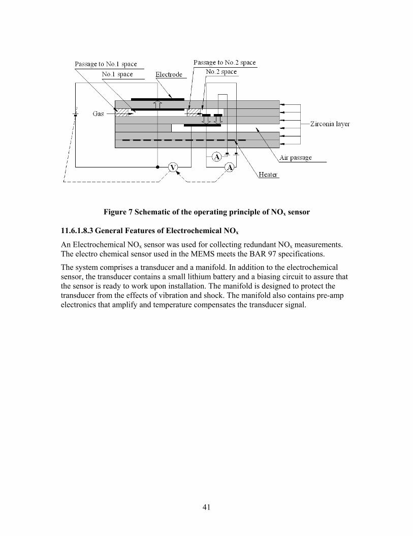
Passage to No.I space

No.I :space

I I I I I I I I

Gas

Electrode

I I I I / L / ------------------~

Passage to No.2 space No.2 space

Heater

Zirconia layer

Air passage

Figure 7 Schematic of the operating principle of NOx sensor

11.6.1.8.3 General Features of Electrochemical NOx

An Electrochemical NOx sensor was used for collecting redundant NOx measurements. The electro chemical sensor used in the MEMS meets the BAR 97 specifications.

The system comprises a transducer and a manifold. In addition to the electrochemical sensor, the transducer contains a small lithium battery and a biasing circuit to assure that the sensor is ready to work upon installation. The manifold is designed to protect the transducer from the effects of vibration and shock. The manifold also contains pre-amp electronics that amplify and temperature compensates the transducer signal.

41

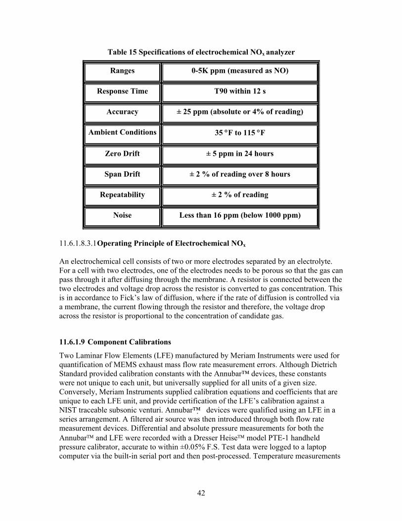
I I

I I

I I

I I

Table 15 Specifications of electrochemical NOx analyzer

Ranges 0-5K ppm (measured as NO)

Response Time T90 within 12 s

Accuracy ± 25 ppm (absolute or 4% of reading)

Ambient Conditions 35 °F to 115 °F

Zero Drift ± 5 ppm in 24 hours

Span Drift ± 2 % of reading over 8 hours

Repeatability ± 2 % of reading

Noise Less than 16 ppm (below 1000 ppm)

11.6.1.8.3.1Operating Principle of Electrochemical NOx

An electrochemical cell consists of two or more electrodes separated by an electrolyte. For a cell with two electrodes, one of the electrodes needs to be porous so that the gas can pass through it after diffusing through the membrane. A resistor is connected between the two electrodes and voltage drop across the resistor is converted to gas concentration. This is in accordance to Fick’s law of diffusion, where if the rate of diffusion is controlled via a membrane, the current flowing through the resistor and therefore, the voltage drop across the resistor is proportional to the concentration of candidate gas.

11.6.1.9 Component Calibrations

Two Laminar Flow Elements (LFE) manufactured by Meriam Instruments were used for quantification of MEMS exhaust mass flow rate measurement errors. Although Dietrich Standard provided calibration constants with the Annubar™ devices, these constants were not unique to each unit, but universally supplied for all units of a given size. Conversely, Meriam Instruments supplied calibration equations and coefficients that are unique to each LFE unit, and provide certification of the LFE’s calibration against a NIST traceable subsonic venturi. Annubar™ devices were qualified using an LFE in a series arrangement. A filtered air source was then introduced through both flow rate measurement devices. Differential and absolute pressure measurements for both the Annubar™ and LFE were recorded with a Dresser Heise™ model PTE-1 handheld pressure calibrator, accurate to within ±0.05% F.S. Test data were logged to a laptop computer via the built-in serial port and then post-processed. Temperature measurements

42

were recorded using J-type thermocouples and Fluke thermocouple readers. The test results substantiated the accuracy figures provided by Dietrich Standard.

The analyzers were calibrated with a Horiba SGD-710C gas divider using gas bottles of know concentrations. The concentrations of gases used were dependent on the maximum concentration in the exhaust of the engine being tested to limit the uncertainty error from the analyzer. Also the calibration gases used were ±1% accurate. A three-way valve was placed at the entrance of the heated sample line, which allowed the calibration line to be connected to the analyzer without removing the heated line. The calibration procedure was performed before each test, which included a zero and a span for the Horiba BE140 and a three-point calibration for the Horiba MEXA 120 and the electrochemical NO cell.

Multi-point calibration curves were developed for the absolute and differential pressure transducers using a Heise™ PTE-1 pressure calibrator. Barometric pressure readings (taken prior to each test) were used to re-set the calibration curve intercepts of the absolute pressure in order to account for sensor drift. Similarly, pre-test calibration also included zeroing the differential pressure transducer.

The relative humidity sensor was calibrated using the RH calibration kit. The procedure used is based on using selected salt solutions to produce a known RH. The method is based on the ASTM standard E104-85 “Standard Practice For Maintaining Constant Relative Humidity by Means of Aqueous Solutions”.

11.6.2 Signal Model 3030PM Hydrocarbon Analyzer

The Signal Model 3030PM is a heated flame ionization detection hydrocarbon analyzer. It was designed to measure organic vapors in combustion stack gases and high dew point samples. The analyzer is equipped with its own sampling pump. A flame ionization detector with a cylindrical collector, flame detector, and igniter are housed in the temperature controlled oven, kept at 675°C. A heated sample line is used to transport the exhaust sample to the analyzer. An electrical signal is produced proportional to the number of carbon atoms present in the sample. For the testing purposes, the analog signal output from Model 3030PM was integrated with the data acquisition system of the EERL. The analog signal was input into the secondary hydrocarbon channel in the EERL data acquisition system. Figure 8 shows a picture of the Signal Model 3030PM.

43

Figure 8 Signal Model 3030PM portable hydrocarbon analyzer

The flame ionization detector works by passing the sample through an ionizing hydrogen flame. The carbon atoms become charged. The ions are then collected onto a polarized electrode outside the combustion zone. The resultant electrical current is proportional to the mass of carbon present in the flame. This electrical current is small and needs to be amplified to produce the signal. The flame fuel is a 40% hydrogen, 60% helium mixture.

The analyzer needs a reference point in order to quantify the concentration of hydrocarbon in the sample. Therefore, a hydrocarbon free sample is provided as the reference. The built-in internal catalyst removes hydrocarbons from ambient air to meet this need. The ambient air is passed over a platinum coated catalyst on an alumina substrate at a high temperature. Zero air is also needed to give a stable signal. The hydrocarbon free air produced by the catalytic process meets this need as well.

There are several features of note for the Signal Model 3030PM. The Model 3030PM has an automatic calibration feature. Signal 3030PM analyzer specifications include 1.5 seconds for 95% response, less than 2% drift in 8 hours, 0.03 ppm propane detector noise, manifold temperature stable at 200°C.

Span gas is provided to the analyzer from a port in the front of the analyzer, and the analyzer generates its own zero air. Zero, span, or both can be re-calculated at any time using the button on the front panel. An automatic calibration can be set, so that zero and span will be re-calculated at a specific time increment. There is also manual zero and span adjustments on the back panel of the analyzer.

The concentration range can be set to values of 0-4, 0-10, 0-40, 0-100, 0-400, 0-1000, 0-4000, and 0-10000ppm ranges. The analog output is from 0-10V. When a specific range

44

is selected, the analyzer automatically sets the low range as 0V, and the high range as 10V. The span gas value must be inputted into the analyzer by setting the span. The value entered must be in methane equivalent form. This is important for the calibration of the analyzer. If the analyzer reads a value for the span gas significantly different from the value that span was set to, it will give an error and the calibration will be aborted. There are also procedures to reset the oven temperature, catalyst temperature, and several other parameters that are not crucial to the operation of the analyzer.

One apparent drawback of the Signal Model 3030PM that is noticeable is that there are lot of features (remote control capabilities, integration capabilities with a RS-232 ports, etc) that are not needed for automotive applications. They are added features that add bulk and unnecessary complexity.

For in-use (in-the-field) applications, power consumption is an important issue. The Signal Model 3030PM is interchangeable between 115VAC and 230VAC +/- 15%, 50 Hz or 60 Hz [9]. The maximum power consumption is 40W. Included in the power specifications are the requirements for the heated line. MEMS currently uses heated lines; therefore, for the integration with MEMS was not a problem.

11.6.3 Simple Portable On-vehicle Testing (SPOT)

11.6.3.1 Introduction

The SPOT system was designed in cooperation with, and under contract to the Assessment and Standards Division of the USEPA, to collect on-vehicle real-time emissions data for use in developing accurate models necessary to define the environmental impact. This information would be useful in determining future emissions regulations.

This unit was designed to be capable of unattended, long duration testing in hostile environmental conditions. These parameters were established to assist in reducing the cost of data collect, allowing a much larger database to be gathered.

The system is comprised of two primary components. The ‘box’ shown in Figure 1, houses the data-logger, cellular modem, GPS, and the sensors for ambient conditions. The box is built from 3/8th inch aluminum, is completely environmentalized, and has 16 rare earth magnets in the base for vehicular attachment. The data-logger utilized 512 Meg flash cards capable of storing the 120 hours of 1hz data.

These units were used, in the recent past, for collecting 100 five-day non-road vehicle tests for the EPA for use in determining new regulations for 2006. The second component is the mass flow detector, pictured below. A single multi-cable connects the box with the mass flow detector.

45

Figure 9 Simple Portable On-vehicle Testing (SPOT) System

Very early in the SPOT developmental stage several devices commercially available for measuring mass flow were tested by AEI. Several of these were based on variations of a Pitot tube. They were found to be inadequate for testing, other than very short-term duration, due to clogging of the small orifices.

The SPOT records the following data:

• Brake-specific NOx

• Exhaust flow rate

• Ambient temperature

• Exhaust temperature

• Relative humidity

• Barometric Pressure

• Engine duty Cycle (engine speed and %load/torque)

• Air-fuel ratio

• GPS tracking

Some of the other features of the SPOT include:

• System installation in less than hour.

46

• Response time (T90) of less than a second

• One week of unattended data acquisition

• Remote monitoring

• OBD-CAN bus J1587, J1939 protocol adaptors

• Rugged construction

• Non-road vehicle data acquisition

• Portable and stationary engine vehicle data acquisition

• On-highway vehicle data acquisition

• Data collection cost could range from $20 to $50.

• Theft resistant.

11.6.3.2 Exhaust Mass Flow rate Measurement

Accurate flow measurement is critical to determining emissions, so AEI developed it’s own proprietary flow device, as shown in Figure 2. This device uses the exhaust flow to create a low-pressure area behind the nosecone, thus inducting outside air. By measuring the flow of “clean” outside air being inducted we are able to utilize a hot wire anemometer and avoid the fouling problem. The induction zone is self-cleaning and has shown no signs of fouling. The measurement of the induction air provides a very accurate determination of exhaust flow. Tests performed at the EPA showed an error factor of only +4% during normal engine operations [10,11].

47

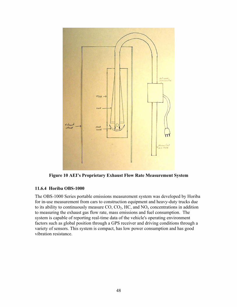
Figure 10 AEI’s Proprietary Exhaust Flow Rate Measurement System

11.6.4 Horiba OBS-1000

The OBS-1000 Series portable emissions measurement system was developed by Horiba for in-use measurement from cars to construction equipment and heavy-duty trucks due to its ability to continuously measure CO, CO2, HC, and NOx concentrations in addition to measuring the exhaust gas flow rate, mass emissions and fuel consumption. The system is capable of reporting real-time data of the vehicle's operating environment factors such as global position through a GPS receiver and driving conditions through a variety of sensors. This system is compact, has low power consumption and has good vibration resistance.

48

Figure 11: Horiba OBS 1000 Series for in-use measurement,

The system includes a non-sampling NOx -A/F analyzer (MEXA 720) and heated NDIR analyzer (MEXA-1170) to measure CO, CO2, and HC. The sampling line for the NDIR analyzer is to be maintained at 120°C. The system utilizes a “tail pipe attachment” that includes a Pitot tube, an exhaust pressure sensor and sensors for longitude, latitude and altitude. A zirconium oxide sensor is used for the NOx-A/F ratio MEXA-720 analyzer, exhaust temperature, air pressure and humidity. A data logger is provided for display. The system comes with a calibration unit for the NOx-A/F sensor. All data are reported on a wet basis and need no water correction. The system does not need an external power supply but requires periodic recharging of the battery pack

Horiba claims that the OBS 1000 Series is compatible with a variety of fuels and vehicle types, including gasoline, diesel, hybrid-fuel, and CNG. The unit requires less than 1 m2

space and weighs around 60 kg.

The OBS-1000 was evaluated using a Mack E7 in an engine test cell. Data was also collected with the WVU MEMS, and laboratory grade analyzers and the CVS in the engine test cell. The engine was operated through the FTP cycle, and over another transient cycle that was developed to faithfully represent on of the on-road routes that were developed for the US EPA and S-HDDE.

11.6.5 Real-Time Particulate Monitor (RPM-100 QCM)

Studies on the RPM-100 resulted in suggestions regarding several modifications to the current RPM-100, which could improve the PM measurement accuracy, repeatability and ‘equivalency’ with the regulatory PM measurement procedures. Following are some of the modifications that need to be made to the system prior to refining the “protocols” for measuring PM with the RPM100 and conducting correlation studies with the CVS and filter-based gravimetric method. However, it was outside the scope of this study to make all the following modifications. The US EPA did accept the following suggestions and requested modifications. Issues related to repeatability will still have to be addressed after the following changes are made.

49

• Operating Temperature: In the current configuration, the operating temperature of the instrument is set at 35 C. However, for the work conducted by US EPA this temperature was raised to 40 C. Although the internal heaters and software would enable higher temperatures to be set at a target of 47 C, the instrument electronics are not currently shielded from the QCM main assembly block and could overheat. Hence, the QCM main assembly needs to be insulated.

• In addition, at these higher operating temperatures, the reference crystal and pressure block need temperature controlling and insulating respectively.

• Automation: The RPM 100 system is currently configured so that it is easy to change from sampling directly into the QCM or from the SCS. However, if heated lines are used (as was the case in the US EPA studies), then the plumbing of the two configurations (direct and from the SCS) needs to be automated by incorporating solenoid controlled valves.

• Additionally, if the test protocol employs the use of humidified air, then a further 2 valves are required to be installed in the system.

• Therefore, the RPM 100 system has to be fitted with 3 controllable valves (utilizing 24 VDC solenoid valves / compressed air) with temperature controlled stainless steel interconnecting lines.

• Flow Measurement: The QCM currently reports volumetric flow. For sampling from the secondary dilution tunnel, it is recommended that the inlet pressure is measured and the flows converted to standard conditions.

• Establish and fine-tune a measurement protocol with the QCM by using HEPA filtered and dew-point generated air to determine mass deposited on the crystal before and after a test. The difference between the pre-test and post-test stabilized mass readings will provide results on the mass of PM. A flavor of measurement protocols for real-time systems is given below.

• The major effort in this task would require several months of bench-top and test cell work. Initially, tests should be conducted on a bench-top to address sensor stabilization, drift, precision and protocol development. This should be followed by an extensive battery of steady-state and transient tests on a CVS tunnel. The results will also highlight the effect of the volatile organics on the QCM mass results. Tests should be conducted on a low-load steady –state mode, possibly a rated speed/10% load.

Preliminary work on protocol development and sensor stabilization was conducted by US EPA with support from MARI. MARI has provided WVU with the RPM 100 and their expertise (time and personnel) at no cost to the project.

Figure 12 and Figure 13 show results from a recent study by the US EPA (at SwRI) on the RPM-100 (QCM). The US EPA purchased the RPM-100 from MARI. Figure 12

50

illustrates the protocol for measuring PM with the RPM-100 (or it could be used with any other real-time PM measurement technique). A considerable amount of work was done at the US EPA, Ann Arbor with the establishing a set of protocols for measuring PM with the TEOM. Figure 13 shows the repeatability of PM data collected with the RPM-100. The following figures illustrate two major points. First, the total PM mass for the complete cycle can be determined by taking a difference of the pre-test and post-test weights. A HEPA filtered sample at a known humidity (22 C and 9.5 C TDew) was drawn across the crystal in the QCM before and after a test, and the mass was allowed to stabilize in both instances. Hence, there exists a strong potential for establishing equivalency with the regulatory requirements where the filters have to be equilibrated before and after each test.

Tests conducted on a backhoe loader (BHL) transient cycle show good test-to-test repeatability with the QCM. The difference between the plateau beyond 1300 seconds and the one before time zero give the total mass collected by the QCM during the test. The steady state plateaus were achieved by passing HEPA filtered air with a known humidity over the crystal. WVU’s experience in other tests has shown that the day-to-day repeatability of the QCM could be a problem. These findings are supported by the Phase II report of the UK PMP Program that was authored by Ricardo, Inc. (2003).

51

-

-

-

-

l

\ \

'

Mas

s (u

g) QCM Real-Time Mass

Low Emission Example, Steady State Mode 3 CRT Trap Emissions

4.5

4.3 1 Protocol 3 4.1

3.9 1 2

Stabilise Mass on QCM at constant Humidity Sample Emissions

3.7 3 Stabilise Mass on QCM at coinstant Humidity

3.5 Sampling Period:

3.3

Slope Derived Concentration 3.1

2 = 0.017 mg/m3 Before / After Mass 2.9

Technigue =0.015 mg/m3

2.7

2.5 6000 6200 6400 6600 6800 7000 7200 7400 7600 7800 8000

Time (s)

Figure 12 Real-Time PM Mass Emissions Signal from CRT Equipped Engine As Measured by an RPM-100.

52

E~::=:::=:::::~::=::;_""'1--_J ___ _J_ ___ _J_ ___ _J_ ___ L _ _J ~ --------+-j

• • X

Mas

s (u

g)

Transient Illustration: BHL "Engine Out" Tests

1 Sampling Period Dilution Ratio 20:1 BHL - 2: Mass 0.61 ug, Conc 1.04 mg/m3

0.5 BHL - 3: Mass 0.61 ug, Conc 1.03 mg/m3 BHL - 4: Mass 0.62 ug, Conc 1.03 mg/m3 BHL-2

BHL-3

0 BHL-4

-0.5

-1

-1.5 -300 -100 100 300 500 700 900 1100 1300 1500

Time

Figure 13 Transient Real-Time PM Mass Emissions Signal from CRT Equipped Engine As Measured by an RPM-100.

53

11.7 Engine Dynamometer Laboratory

This section describes the engine test cell facility at the WVU EERL. The engine facility is in compliance with the requirements of 40 CFR, Part 89, 40 CFR Part 86, the Subpart N-Emission Regulations for Heavy-Duty Diesel Engines and the Gaseous and Particulate Exhaust Test Procedures, 30 CFR, and ISO 8178. Appendix D outlines WVU’s Quality Control and Quality Assurance Plan.

11.7.1 Dynamometer/Dynamometer Control

In order to simulate real-world loading conditions on an engine in a laboratory environment, a dynamometer, or power absorber, is used. Engine testing is generally performed with one of three basic types of dynamometers. In order to familiarize the reader with the basic principles of operation, the following discussion has been included.

11.7.1.1 Eddy-Current Dynamometers

Air-cooled eddy current dynamometers operate by establishing a magnetic field by energizing a set of stationary coils with DC power. Iron rotors, which are attached to the output shaft of the test engine, rotate in the magnetic field and generate eddy currents in the rotors, which produce a counter force to the direction of rotational motion. The power applied to the dynamometer and the speed at which it is rotating. The absorbed energy is converted into heat in the two externally located rotors, which are designed with curvilinear cooling fins for fast heat dissipation. The windage losses associated with this cooling are compensated for during data reduction.

11.7.1.2 Electric Dynamometers

Electric dynamometer operate much like electric motors. In fact, to start the test engine, the dynamometer is operated as an electric motor, while the fuel (for compression-ignition engines) or ignition (for spark-ignition engines) sources for the test engines are disabled. In such a motoring configuration, the parasitic, or fractional, losses of the engine can be measured and simulations of coast-down may be performed. Once the fuel or ignition source for the engine is activated, the dynamometer may be used to load the engine by operating in the same manner as a generator. Torque is developed due to the magnetic coupling between the armature and stator. The engine output is then determined from a side-arm load cell that is attached between the stator housing and the dynamometer-mounting frame. The load applied to the engine is varied by strengthening the field voltage or reducing the load resistance.

11.7.2 Test Dynamometer Specifications

All in-laboratory testing performed in this study utilized both eddy-current and electric (DC dynamometer) dynamometers.

54

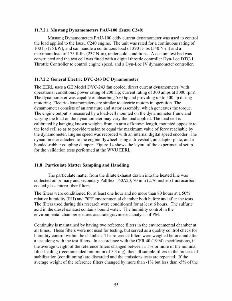
11.7.2.1 Mustang Dynamometers PAU-100 (Isuzu C240)

Mustang Dynamometers PAU-100 eddy current dynamometer was used to control the load applied to the Isuzu C240 engine. The unit was rated for a continuous rating of 100 hp (75 kW), and can handle a continuous load of 390 ft-lbs (540 N-m) and a maximum load of 175 ft-lbs (237 N-m), under cold conditions. A custom test bed was constructed and the test cell was fitted with a digital throttle controller Dyn-Loc DTC-1 Throttle Controller to control engine speed, and a Dyn-Loc IV dynamometer controller.

11.7.2.2 General Electric DYC-243 DC Dynamometer

The EERL uses a GE Model DYC-243 fan cooled, direct current dynamometer (with operational conditions: power rating of 200 Hp; current rating of 300 amps at 3000 rpm). The dynamometer was capable of absorbing 550 hp and providing up to 500 hp during motoring. Electric dynamometers are similar to electric motors in operation. The dynamometer consists of an armature and stator assembly, which generates the torque. The engine output is measured by a load-cell mounted on the dynamometer frame and varying the load on the dynamometer may vary the load applied. The load cell is calibrated by hanging known weights from an arm of known length, mounted opposite to the load cell so as to provide tension to equal the maximum value of force reachable by the dynamometer. Engine speed was recorded with an internal digital speed encoder. The dynamometer attached to the engine flywheel using a driveshaft, an adapter plate, and a bonded-rubber coupling damper. Figure 14 shows the layout of the experimental setup for the validation tests performed at the WVU EERL.

11.8 Particulate Matter Sampling and Handling

The particulate matter from the dilute exhaust drawn into the heated line was collected on primary and secondary Pallflex T60A20, 70 mm (2.76 inches) fluorocarbon coated glass micro fiber filters.

The filters were conditioned for at least one hour and no more than 80 hours at a 50% relative humidity (RH) and 70°F environmental chamber both before and after the tests. The filters used during this research were conditioned for at least 6 hours. The sulfuric acid in the diesel exhaust contains bound water. The humidity control in the environmental chamber ensures accurate gravimetric analysis of PM.

Continuity is maintained by having two reference filters in the environmental chamber at all times. These filters were not used for testing, but served as a quality control check for humidity control within the chamber. The reference filters were weighed before and after a test along with the test filters. In accordance with the CFR 40 (1994) specifications, if the average weight of the reference filters changed between ± 5% or more of the nominal filter loading (recommended minimum of 5.3 mg), then all sample filters in the process of stabilization (conditioning) are discarded and the emissions tests are repeated. If the average weight of the reference filters changed by more than -1% but less than -5% of the

55

CJ 10000000000000000001

Heo. ted Line

00

Fuel Meter

Dilution Air

--I>

~--,~-- M5 Pitot Tube

Engine

Dynar1or1eter

Pririory Dilution TunnelCinsuln ted)

00 @ @

M5 Control Console

Model 955 Cheriiluriinescent N x Analyzer

c=J [[J [[J

77 ~

Heated Line

Heated Line

IEHE I 1EHE~ 00000 [[J O [[J O [[J O [[J O [[J 0

F1ve-'way Valves and Flow Meters

Venturi

Purip

Stec Model SGD-710 GAS Divider

T

P

P

T

P T

P

P

Figure 14 of West Virginia University’s Engine and Emissions Research Laboratory Emissions Measurement System

56

nominal filter loading, then two options are given - either repeat the emissions test or add the amount of weight loss to the net weight of the sample. If the difference in the reference filter weights changed more than 1% but less than 5% of the nominal filter loading, then the option is given of either repeating the emissions test or accepting the measured sample filter weight values. If the weight of the reference filters changed by less than ± 1%, then the measured sample weight was used.

The particulate filters, reference and sample, were stored in glass petri dishes, while conditioning in the environmental chamber. These dishes were covered but not sealed to prevent dust from accumulating on the filters while allowing humidity exchange to take place. WVU uses glass petri dishes instead of plastic petri dishes because the static electric charge carried by the plastic petri dishes could result in the loss of particulate matter from the filter.

Even though the dilution air was filtered before entering the primary or the secondary dilution tunnels, background samples were taken. The procedure required placing a weighed and conditioned filter in the primary position of the filter, holding and pulling a metered sample of the ambient air across the filter, post conditioning and weighing of the filter, and subtracting the weight from the sample filters.

The total particulate matter (TPM) was determined by weighing the filters before and after each test after conditioning. A Cahn 32 microbalance was used for weighing the filters. The microbalance had a remote weighing chamber that was placed inside the environmental chamber on a vibration isolation table, while the electronic unit was left outside of the chamber. The balance had a 3.5 g weighing capacity with three weighing ranges and a sensitivity of 0.1 µg.

11.8.1 Dilution Tunnel

The purpose of the dilution tunnel is to dilute an engine’s raw exhaust gas with fresh ambient air so as to simulate the emission of exhaust in real world conditions and to aid in the emissions sampling process. Since it is necessary to determine what effect this diluted exhaust will have on humans, it is necessary to simulate the real world conditions in a laboratory by using a dilution tunnel. In some instances, the dilution air may be conditioned before it is mixed with the exhaust and it may consist of filtration systems (to remove particulate matter from the air) and humidity and temperature control. An alternative to this is to measure the level of background PM and subtract it from the value obtained from the exhaust sample. Diluting the raw exhaust with fresh ambient air lowers the dew point temperature, which prevents water condensation. Water condensation would cause the loss of certain gaseous components (for example, NO2) and hence, compromise the exhaust emissions results. Water condensation affects certain instruments, such as the non-dispersive infrared analyzers and the particulate matter measurements would also be affected. In a study about laboratory variability in exhaust measurements it was found that in each of the engine laboratories studied, there were a variety of dilution tunnel designs. Differences included tunnel diameter, tunnel length, method of mixing, flow rate, and the length from point of exhaust injection to the sampling zone. The dilution tunnels used in the WVU laboratory are a double dilution type. The dilution tunnel is eighteen inches in diameter and has a total length of twenty

57

feet. The dilution tunnel uses an eight inch orifice placed three feet from the beginning of the tunnel. The orifice insures that the dilute exhaust mixture is thoroughly mixed by the time it reaches the sampling zone; ten diameters downstream, so that the gaseous and particulate probes will pull in a representative sample.

11.8.2 Critical Flow Venturi

In compliance with the 40 CFR Part 86, Subpart N, a constant volume sampler (CVS) was used to draw the diluted exhaust through the dilution tunnel. The CVS system operates based on the theory of critical flow nozzles. A critical flow venturi (CFV) is placed upstream of a blower, which pulls the diluted exhaust mixture at a constant mass flow rate once the venturi is under sonic conditions, or choked flow conditions.

This design was based upon the fact that the flow rate of a gas, under choked conditions, through a critical flow venturi is controlled by the diameter of the throat and the upstream flow conditions. The CFV-CVS system has a critical venturi installed in line with a 55.9 kW (75 hp) centrifugal blower. The constant volume sampling system has four different venturis, three of which have a design flowrate of 28.3 m3/min. (1000 scfm) and the fourth has a design flowrate of 11.32 m3/min. (400 scfm). A maximum tunnel flowrate of 3400 scfm can be achieved by using this system.

The critical flow venturi allows for the measurement of the mass flow rate (flow rate in standard cubic feet per minute at standard conditions of 20°C, 101.3 kPa (68°F, 29.92 in Hg) of diluted exhaust by monitoring the upstream absolute pressure (P) with a Viatran absolute pressure transducer, Model No 1042 AC3AAA20 and temperature (T) with a 3-wire resistive temperature device by Tayco Model No. 68-3839. The mass flow rate was then calculated as a function of CFV calibration coefficient, absolute pressure and absolute temperature at the venturi inlet.

11.8.3 Secondary Dilution Tunnel and Particulate Sampling

The process of measuring the emissions of particulate matter from diesel engines consists of conveying the exhaust to a dilution tunnel (single or double) in which the exhaust is diluted with air and cooled to a temperature not exceeding 51.7°C (125°F), obtaining a representative sample of the particulate matter in the dilute sample by filtration, and then determining the mass collected on the filter or filters. The WVU facility uses the double dilution method for particulate matter sampling. The double dilution method draws a proportional sample of diluted exhaust from the primary tunnel and dilutes it further in the secondary dilution tunnel. The sample then passes through two, a primary and a secondary, Pallflex 70 mm (2.76 inches) fluorocarbon coated micro fiber glass filters, T60A20, which collect the particulate matter.

The particulate sampling system was designed to perform in accordance with the 40 CFR Part 86. The secondary dilution tunnel is required to maintain the double diluted exhaust stream at a temperature of 51.7°C (125°F) or less immediately before the primary particulate filter in the secondary dilution tunnel. Particulate Matter (PM) collected from

58

a dilution tunnel is influenced by the conditions at which the tunnel is operated, most significant being the temperature and dilution ratio.

The exhaust sample is drawn through a 1.3 cm (0.5 inches) diameter transfer tube located at the sampling zone in the primary dilution tunnel. The inlet faces upstream and is approximately 17.8 cm (7 inches) in length. The total flow and the secondary dilution air flow through the secondary tunnel is controlled by two Sierra 740-L-1 series mass flow controllers and two Gast series 1023-101Q-583X rotary vane pumps. A Roots positive displacement flow meter provides an additional check on the total flow through the PM filters. The total flow ranges from 0 lpm to 170 lpm (0 scfm to 6 scfm) while secondary dilution air flow ranges from 0 lpm to 85 lpm (0 scfm to 3 scfm). During testing, flow through the secondary dilution tunnel varies in proportion to the flow through the primary dilution tunnel. The mass flow controllers were calibrated using a Meriam Instruments laminar flow element (LFE) Model No. 50MW20, rated at 0 m3/min to 6.52 m3/min (0 scfm to 23 scfm).

The secondary dilution tunnel is 7.62 cm (3.0 inches) in diameter and 76.2 cm (30 inches) long. This provides sufficient time for the exhaust sample to be mixed with the dilution air and to reach a temperature of 51.7°C (125°F). A stainless steel filter holder with the primary and secondary filters is connected at the end of the secondary dilution tunnel. The filter holder is constructed of stainless steel to prevent reactions with the corrosive exhaust sample and is designed to allow easy access to the filters.

11.8.4 Gas Analysis System

A gas analysis bench was used to measure the concentration of gaseous components in a diluted exhaust gas stream from the heavy-duty diesel engine. The gas analysis bench consists of four major components: CO2 analyzer, CO analyzer, NOx analyzer, and a HC analyzer. The gaseous samples are taken 10 diameters downstream of the mixing zone in the primary dilution tunnel to allow for development of the turbulent duct flow. Four heated stainless steel probes are inserted into the dilution tunnel at the sampling zone at a depth of approximately six inches. These probes are connected to heated lines, which transfer the gaseous samples to their respective analyzers. The hydrocarbon line and probe are kept at a wall temperature of 191°C ± 6°C (375°F ±10°F) while the other probes and lines are kept at 113°C ± 6°C (235°F±10°F) at the wall. The temperatures were kept high in order to prevent water condensation, which would have affected the measurements by the analyzers. In case of hydrocarbon probe and line, the temperature is maintained at 191°C (375°F) to prevent the higher-molecular weight hydrocarbons from condensing out on the walls and other surfaces in the sampling stream.

11.8.4.1 Hydrocarbon Analyzer

The hydrocarbon analyzer is a Rosemount Analytical Model 402 heated flame ionization detector (HFID) and operates on the following principle. The sensor is a burner where a regulated flow of sample gas flows through a flame produced by regulated flows of air and a pre-mixed hydrogen/helium fuel gas. Polarized electrodes then collect the ions that are produced causing current to flow through the associated electronic measuring

59

circuitry. The current flow is proportional to the rate at which carbon atoms enter the burner.

11.8.4.2 CO/CO2 Analyzer

The CO and CO2 analyzers were Horiba Model AIA–210LE and Horiba Model AIA-210 Non-Dispersive Infrared (NDIR) analyzers respectively. The NDIR uses the exhaust gas species being measured to detect itself by the principle of selective absorption, which means that the infrared energy of a particular wavelength, specific to a certain gas, will be absorbed by that gas. Infrared energy of other wavelengths will be transmitted by that gas, just as the absorbed wavelength will be transmitted by other gases.

11.8.4.3 NOx Analyzer

The NO/NOx analyzer used is a Rosemount Model 955 Chemiluminescent Analyzer. The analyzer can determine the concentration of either NO or NO + NO2 which together is called NOx. For the determination of NO, the sample NO is quantitatively converted into NO2 by gas-phase oxidation with molecular ozone which is generated inside the analyzer by an ozone generator, which is supplied with the external bottled air supply. When this reaction takes place, approximately 10% of the NO2 molecules are elevated to an electronically excited state followed by immediate reversion to the non-excited state accompanied by a photon emission. The instrument response is proportional to the total NO in the converted sample. The operation for NOx is identical to that of NO except that the gas sample stream is first passed through a converter, which converts the NO2 into NO. In this case, the instrument response is proportional to the NO present in the original sample plus the NO produced by the dissociation of NO2.

11.8.4.4 Bag Sampling

Although continuous samples were taken of the regulated exhaust gases, bag samples of dilute exhaust and dilution (background concentration) air were also taken. These samples were collected in separate 80-liter Tedlar bags. Once the test was completed, the bag samples were hooked up to the gas analyzers and their respective concentrations were measured and then the bags were evacuated and reset for the next test.

The background or ambient air concentrations of the regulated emissions were used to correct the dilute exhaust bag sample and the continuous sample readings. The dilute sample served only as a quality control/quality assurance check, which provided a way to compare the results with the continuous sample.

11.8.5 Instrumentation Control and Data Acquisition

The software used in the study was already developed and installed in the EERL. The program utilized an RTI-815F data acquisition board and a rack mounted signal conditioning board comprised of a number of Analog Devices 3B series conditioning modules.

60

The data acquisition programs acquired the raw data in the form of ADC codes and another program converted the raw data into proper engineering units. The program then wrote the final data to a file.

11.9 Partial-flow Dilution Tunnel

A portable partial-flow dilution tunnel (mini-tunnel) was used for gravimetric analysis of PM emissions. The exhaust gas is treated the same as in a full-flow CVS system, but only a portion of the total exhaust gas enters the tunnel. Some manufacturers refer to smaller versions of this design as a micro-tunnel, with the only distinction being tunnel size. Additionally, one manufacturer may use the name micro-tunnel where another would use mini-tunnel for the same size system. Therefore, throughout the text, and associated literature, partial-flow dilution, mini-dilution, and micro-dilution may be encountered as interchangeable terminology.

The mini-tunnel used is of a partial-flow design [7], where a known amount of raw exhaust gas sample is routed into the tunnel via a heated line and is mixed with metered HEPA-filtered, and temperature and humidity conditioned dilution air in order to achieve desired dilution ratios. The dilution ratio is controlled via a computer program using inputs from two mass flow controllers (flow based dilution ratio control) or time-aligned raw and dilute CO2 concentrations obtained using a two-channel CO2 analyzer (CO2 based dilution ratio control). The dilution air flow rate and the total diluted exhaust flow rate (sum of raw exhaust sample flow rate and dilution air flow rate) through the mini-tunnel are controlled with Sierra mass flow controllers. In the case of CO2 based dilution ratio control, raw and dilute CO2 measurements are used as inputs to a closed loop control system to obtain the desired dilution ratio. In the case of the validation tests conducted in the lab, some of the tests were conducted using flow based dilution ratio control and some of them were conducted using CO2 based dilution ratio control.

The exhaust, sampling, sample conditioning, and sample dilution systems are mounted on the PM cart. A schematic of the cart is shown in Figure 15.

The dilution tunnel is approximately 0.05m (2”) in diameter and 0.61m (24”) in length and is constructed of stainless steel to prevent corrosion. The mini-tunnel design is in compliance with the requirements of ISO 8178-1:1996(E) 16.1.1. The dilution air is provided to the tunnel by a rotary-vane pump. The dilution air is pumped through a HEPA-filter, and then passed through a heat exchanger and a chiller to regulate its temperature and humidity. Temperature is maintained as close as possible to ambient temperature prior to entering the mass flow controller.

The raw exhaust gas sample enters the tunnel along its centerline and passes through a mixing orifice plate that is close-coupled to the divergent tunnel entrance. The orifice plate creates turbulence in the flow path that promotes thorough mixing. The tunnel flow rates are maintained sufficiently high in order to obtain the fully developed, blunt-shaped turbulent flow profile that reduces the sensitivity of sample probe placement. A second rotary-vane pump draws the entire tunnel flow stream across a stainless steel filter holder which contains two Pallflex 70mm diameter Model T60A20 fluorocarbon coated glass micro fiber filters.

61

The diluted exhaust flow across the filters is metered through a mass flow controller. The diluted sample stream is maintained at temperatures below 125oF, measured at the inlet of the stainless steel filter holder.

A mass flow controller downstream of the filter controls the total flow rate through the tunnel. A 3-way ball valve fitted between the tunnel exit and the stainless steel filter holder serves to bypass the tunnel flow stream for the time during which PM data was not being taken. The two Sierra mass flow controllers provide flow rate control of the total flow and dilution air flow based on computer voltage outputs determined from the raw and dilute CO2 concentrations. The mass flow controllers are routinely recalibrated by the manufacturer and are additionally checked in-house with Merriam Instruments laminar flow element.

The dilution ratio is continuously controlled and maintained at the target value using the dilute and raw CO2 concentration measurements in the dilution tunnel. Exhaust sample flow rate into the tunnel is inferred from this dilution ratio along with the total mass flow rate measured using the mass flow controller.

The PM samples are collected on filters during each mode of engine testing. The PM collected on filters consists primarily of elemental carbon as well as sulfates, soluble organic fraction (SOF), engine wear metal and bound water. The sample filters are conditioned in an environmentally controlled chamber to 70oF and 50% relative humidity, in compliance with requirements of 40 CFR Parts 86 and 89, and weighed before and after sample collection using a Cahn C-32 microbalance, a 40 CFR Part 86 compliant microbalance.

62

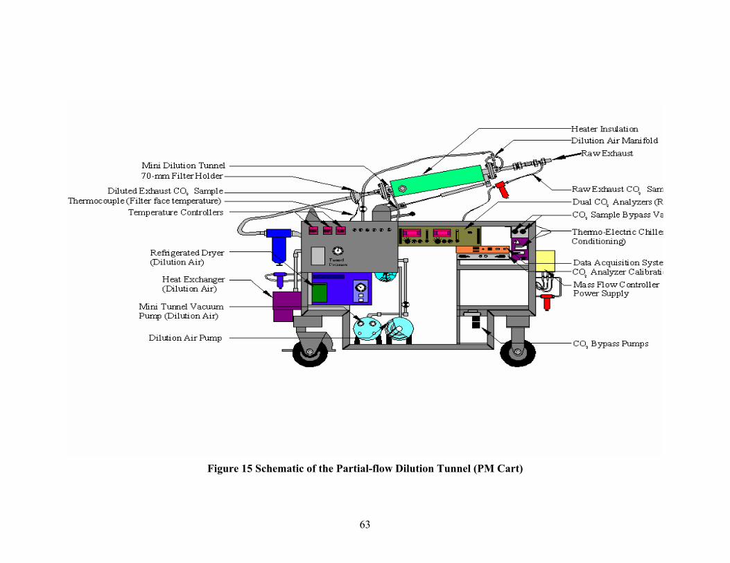
Mini Dilution Tunnel -------------~ 70-mmFilterHolder------~~

Diluted Ex!Bust CO, Sample--------------==:N;--,l/:,~:\.\"L::~Thermoc oupl e (Filter face temperature)

Temperature Controll ers

Refrigerated D,yer ---(Di! ution Air)

Heat Exchanger (Dilution Air)

Mini Tunnel Vacuum ----Pump (Dilution Air)

Dilution Air Pump

~---------Heater Insulation

,------Dilution Air Manifold

RawExlBust cq Sam

,-------Dual CO. Analyzers (R

~~--CO, Sample Bypass Va

Thermo-Electric Chille, Conditioning)

Data Acquisition Syste cq Analyzer Calibrati,

~--- CO, Bypass Pumps

Figure 15 Schematic of the Partial-flow Dilution Tunnel (PM Cart)

63

11.10 Method 5 Analysis:

11.10.1 Principle and operation:

Gravimetric analysis of particulate matter PM emissions from stationary sources, has been performed for regulatory purposes using the Method 5

In this method, PM from engine is sampled isokinetically and collected on a filter which is maintained at 250°F. The water vapor in the exhaust gas along with any condensed organics are removed downstream of the filter - in impingers immersed in an ice bath. The sample gas leaving the impingers is then drawn through a felt filter, to remove any foreign matter, before entering the sampling pump. The outlet of the pump is connected to the control console that comprises a dry gas meter to measure sample volume and a calibrated orifice. The sample gas exits the control console through the calibrated orifice. A U-tube manometer is connected across the calibrated orifice to provide a reference to control sample flowrate. Isokinetic sampling is achieved by comparing the Pitot tube differential pressure (∆P), provided by a type S Pitot tube inserted eight diameters downstream of the sampling nozzle, with the dry gas meter orifice differential pressure reading (∆H) and then adjusting the orifice differential pressure (∆H) to the desired value. Details of the Method 5 sampling train, as well as associated theories and data analysis is included in Appendix E.

It should be noted that other regulatory bodies, such as, the US EPA, do not consider the back half for determination of TPM. Only the front half, that is, “probe catch” and “filter catch” are required to define TPM. It should also be noted that there is a separate method, outlined in Method 202 – “Determination of Condensable Particulate Emissions from Stationary Sources”, that governs the extraction of the back half contents.

It should be noted that proportional sampling was conducted to collect total particulate matter from the CVS. Tests were conducted on Isuzu C240 over the R 100 (Rated speed and 100% load) and I 100 (Intermediate speed and 100% load) mode, and also on the DDC Series 50 engine over the I50 (Intermediate speed and 50% load) and I75 (Intermediate speed and 75% load) modes of engine operation. PM analysis was conducted and with and without the back-half. The filter catch was added to the probe catch to obtain the total PM.

Shown below are the front view and side view of the Method 5 sampling train, which was installed on the exhaust stack of the Isuzu C240 engine.

64

Figure 16 Front view of the Method 5 sampling system

Figure 17 Lateral view of the Method 5 sampling system. Pitot tubes used for exhaust flow rate measurement can be seen on the left.

65

11.11 Modified Method 5 Test:

Based upon results from our Method 5 tests, and subsequent discussions with CARB, this program attempted to determine whether a modification to the Method 5 would yield valid results that could ease the use of Method 5 sampling train in the field. The goal of this exercise was to determine if the existing Method 5 sampling trains could be employed to determine PM emissions in a convenient, yet accurate manner, which would yield results similar to what regulatory PM method used in an engine certification test.

WVU determined that the total PM measured with the CVS, in accordance with the requirements of ISO-8178, and 40 CFR, Part 89, was in very good agreement with the front-half of the Method 5 test protocols. WVU’s findings are supported by the study conducted by researchers at CE-CERT, University of California, Riverside. As a result, WVU employed a multi-hole sampling probe that spanned the entire diameter of the exhaust stack, instead of a gooseneck nozzle, and maintained the sampling probe at ambient temperatures and at 250ºF. The filter holder, which is located inside the filter box of the Method 5 sampling train, was maintained at the recommended temperature of 250º F, and also at ambient conditions. A test matrix for the study is below in Table 16.

A few simple additional tests using the Method 5 sampling system were also performed to investigate the effect of not pre-conditioning the PM filters. A test matrix for the study is below in Table 16 on page 65. For these tests, a DDC Series 60 was operated at the conditions given in Table 16 (intermediate speed and 50% and 75% load). The meaning of the phrase “not preconditioning” for the PM filters is explained in section of 13.7.1 . The filters, placed in unsealed glass petri dishes, were first conditioned according to the regulatory requirements (CFR 40, Part 86, subpart N) in an environmental chamber for 8 hours and weighed. They were then taken outside the environmental chamber and conditioned to the local conditions in the unsealed Petri dishes that permitted humidity exchanges. This was done to mimic the equilibration of in-field test filters in uncontrolled environments (during pre- and post-test). They were then used for testing. After the tests, the filters were then allowed to condition under local conditions for two days (to mimic the time required to ship the filters back) and then taken to environmental chamber to undergo conditioning according to regulatory requirements. The filters were then weighed after they had been conditioned to the set humidity and temperature. Thus, the entire sub-test would approximate remote filter usage of filters that were pre- and post-weighed at a laboratory location.

66

Table 16: Test Matrix for the Additional Set of Method 5 Tests

Mode Test

#

Probe

Temperature

Filter box

Temperature

Sampling

nozzle

Method 5 Filter

conditions

I 50

1

Base

-line

250°F 250°F

Multihole

averaging

nozzle.

Pre-conditioned at 50%

Relative Humidity and

75°F temperature

2 Repeat Test # 1

3 Ambient

temperature

Ambient

temperature

Multihole

averaging

nozzle.



75°F temperature

4 Repeat Test # 3

5 Ambient

temperature

Ambient

temperature

Multihole

averaging

nozzle.

No Pre-conditioning for

filters

6 Repeat Test # 5

I 75

7

Base

line

250°F 250°F

Multihole

averaging

nozzle.



75°F temperature

8 Repeat Test # 7

9 Ambient

temperature

Ambient

temperature

Multihole

averaging

nozzle.



75°F temperature

10 Repeat Test # 9

11 Ambient

temperature

Ambient

temperature

Multihole

averaging

nozzle.

No Pre-conditioning for

filters

12 Repeat Test # 11

67

In the second set of the experiments, the temperature controller for the probe liner and the filter box were turned-off. Other parameters were the same as those in the first set of experiments. The results obtained in this set of experiments could be compared with those obtained in the first set.

The purpose of the third set of tests was to quantify the effect of not pre-conditioning the filters. This information could be used while doing in-field tests where it may not be possible to pre-condition these filters. The results obtained in this set may be compared with the results obtained in the second set.

Tests were then repeated for the I 75 (75 % load at intermediate speed) engine operating condition.

11.12 DESIGN OF NOx CONVERTER

11.12.1 Introduction

The external NOx converter (NO2 to NO) was used in the MEMS to condition the sample stream upstream of the NOx analyzer. In exhaust streams of diesel engines equipped with catalyzed diesel particulate filters (DPFs), NO2 forms a relatively large portion of NOx. In diesel engines without DPFs, NO2 may constitute 3% to 10% of total NOx – possibly more for air/fuel ratios exceeding 60:1. It should be noted that currently exhaust gas analyzers and the MEXA-120 NOx analyzer which is used in the MEMS has a varying response to NO2 depending upon the NO2 concentration. Hence, there arises a need to have a NOx converter to obtain accurate measurements of the total oxides of nitrogen (NOx). Various configurations of the sampling system were tested to obtain highest conversion efficiency for the converter.

11.12.2 Design of the NOx Converter

Various designs were considered for the NOx converter. Some of the problems that were encountered in the design of the converter were maintaining a high flow rate through the converter, proper heating of the catalyst and positioning of the NOx sensor. The final design of the converter that was used in the version of MEMS that was used in this study is shown in Figure 18 below.

68

Figure 18 WVU-MEMS NOx converter

11.12.3 Need for a Converter Catalyst

For a reaction to take place there have to be collisions occurring between reactant molecules or atoms. Collisions only result in a reaction if the particles collide with enough energy to get the reaction started. This minimum energy required is called the activation energy for the reaction. A catalyst affects the rate of reaction, by reducing the activation energy and remains chemically unchanged at the end of the reaction. Converter catalysts are transition metals and their oxides suspended on a matrix of ceramic material designed to offer the exhaust gases an enormous surface area as they pass through. The metal/metal oxide catalysts lower the activation energy necessary to get to the transition state and increase the rate of the reverse reaction.

11.12.4 Catalyst for the NOx converter

There are a number of commercially available catalysts that are used for the conversion of NO2 to NO. Efficiency tests were done on some of the catalysts using the MEMS system. Finally, the Horiba NOx (Mo/Vitreous Carbon) catalyst was chosen for use in the converter. Table 17 lists two of the catalysts that were tested and their sources.

69

Table 17 Catalysts used for the converter testing

Catalyst Name Source

A Horiba Catalyst (Mo/Vitreous

Carbon) Horiba Inc.

B Vitreous Carbon Rosemount Analytical Inc.

11.12.5 Effect of the Sampling System Configuration on the Conversion

efficiency of the NOx Converter

Experiments were performed with the converter to evaluate the effect of the sampling system configuration on the conversion efficiency. This was an effort to determine the optimum operating conditions for the maximum converter efficiency during in-use testing.

The first set of tests was performed to evaluate the effect of varying sampling line temperature on conversion efficiency. The sample flow rate through each catalyst was kept constant (fixed sampling residence time). Tests were repeated on both the catalysts. An NO2 bottle of 600ppm concentration was used for testing purposes. The MEXA 120 analyzer was calibrated using NO with a 1000ppm concentration.

For the next set of tests the sample line temperatures were maintained constant, and the flow rate was varied. The following Table 18 gives the test matrix that was followed in performing the efficiency tests.

70

-.. •

.. • • .. ..

II II II II II II II II II II II II II

' ......

.. ....

II II II II II II II II II II II II II

...

E7 ~

I I I I I I I I I I I I I

Table 18 Sampling conditions for the NOx converter

Catalyst Temperature (°F) Flow rate (lpm) A 300 3.0 A 325 3.0 A 350 3.0 B 300 3.0 B 325 3.0 B 350 3.0 A 300 3.5 A 325 3.5 A 350 3.5 B 300 3.5 B 325 3.5 B 350 3.5

Con

vers

ion

Effic

ienc

y (%

)

100

95

90

85

80

75

300 F 325 F 350 F

100 200 300 400 500 600 700

Input NO2 Concentration (ppm)

Figure 19 Comparison of the NOx converter efficiency with a flow rate of 3.0 lpm at temperatures of 300° F, 325° F and 350° F using Horiba catalyst.

71

E -

- ----. - --- .............. --- ~ ----~

100 C

onve

rsio

n E

ffici

ency

(%)

95

90

85

80

75

300 F 325 F 350 F

100 200 300 400 500 600 700


Figure 20 Comparison of the NOx converter efficiency with a flow rate of 3.5 lpm at temperatures of 300° F, 325° F and 350° F using Horiba catalyst.

100

Con

vers

ion

Effi

cien

cy (%

)

95

90

85

80

75

300 F 325 F 350 F

100 200 300 400 500 600 700


Figure 21 Comparison of the NOx converter efficiency with a flow rate of 3.0 lpm at temperatures of 300° F, 325° F and 350° F using Vitreous Carbon catalyst.

72

75

80

85

90

95

100 C

onve

rsio

n E

ffici

ency

(%)

300 F 325 F 350 F

------------------ ---

100 200 300 400 500 600 700


Figure 22 Comparison of the NOx converter efficiency with a flow rate of 3.5 lpm at temperatures of 300° F, 325° F and 350° F using Vitreous Carbon catalyst.

11.12.6 Inference on the Optimum Conditions for the NOx converter

Results of the various tests discussed in 11.12.5 are shown in Figure 19 to Figure 22 and the results suggest that the NOx converter efficiency is strongly dependent upon catalyst temperature and the residence time (flow rate). The converter efficiency was greater than 95% for NO2 concentrations less than 100 ppm. For concentrations in the range of 100-300 ppm the converter efficiency was close to 90%. For concentrations greater than 300 ppm the efficiency was about 80-85%.

It can be seen from Figure 19 to Figure 22 that the maximum converter efficiencies were obtained with a converter consisting of the Horiba catalyst, which was maintained at a temperature of 350°F, and a sample flow rate of 3.0 lpm.

73

11.13 ON-ROAD ROUTES

In order to validate the proposed fuel-specific emissions based test method, WVU employed its experience in on-road, on-board emissions evaluation from heavy-duty trucks. This validation was performed using on-board testing of on-highway vehicles rather than stationary or portable engines because WVU had concurrent testing which facilitated the data collection. These particular test engines provided WVU with the means to have a more accurate comparison, since measured brake-specific CO2 data (as well as BSFC data) was available, as opposed to advertised or manufacturer reported data. Moreover, the engines could be tested in-field as well as in the emissions laboratory. WVU holds that the use of these on-highway engines does not significantly affect the conclusions and recommendations formed regarding the test methodology developed under this study.

Using the MEMS unit that is capable of measuring brake-specific emissions (that is, capable of measuring exhaust flowrate, engine speed, percent load, and emissions concentrations), and test protocols approved by the US EPA and the S-HDDE, researchers conducted tests on a Class-8 tractor with a MY 1997 engine. Please note that information on the test engine is not provided for confidentiality reasons as requested by Cummins, Inc. Brake-specific emissions of NOx and CO2 were employed to develop ratios of bsNOx/bsCO2 which were then compared with concentration ratios of NOx/CO2. The goal of this exercise was to develop and verify the proposed concept of using a “Compliance Factor” for in-field emissions measurement for compliance purposes. Test routes are briefly described below.

11.13.1 Saltwell, WV

This route was split into inbound and return journeys. The route originated at the WVU Sabraton facility (Greater Morgantown Area) close to an entrance ramp accessing I-68 west. The route proceeded to I-79, and followed I-79 south to the turnaround point at the I-79 Saltwell Rd. Exit (near Clarksburg, WV). The total distance was 58.7 miles. The interstate was posted at 70 mph, but there were two curves with advisory signs below that speed. The outbound leg was designated SAB2SW and the return leg was designated SW2SAB.

74

Figure 23 The Saltwell Route is indicated by the yellow highlighted section of the map. The full route was a round-trip drive driven in two legs. The first leg was from Morgantown to the Saltwell Rd. exit and the second leg was the return trip.

11.13.2 Bruceton Mills, WV

This route was divided into outbound and return journeys. The route originated at the WVU Sabraton facility (Greater Morgantown Area) close to an entrance ramp on I-68 east, and continued on I-68 where a climb of a sustained 5% grade existed, followed by transient road grades to the turnaround point at Bruceton Mills, WV. The total distance was 39.7 miles. The interstate was posted at 70 mph, but the 5% descent on the return journey was posted at 50 mph for trucks and was preceded by a mandatory truck stop for checking brakes. In the high-speed freeway operation, dramatic reductions in vehicle speed were encountered as the vehicle climbed hills along the route. In the case of this route, truck speed restrictions and necessary precautions during steep descent on the return leg of the journey reduced the operating speed on I-68 westbound. The outbound leg was designated as SAB2BM and the return leg was designated as BM2SAB.

75

Figure 24 The Bruceton Mills Route is indicated by the yellow highlighted section of the map. The full route was a round-trip drive driven in two legs. Morgantown to Bruceton Mills was the first leg and Bruceton Mills to Morgantown was the second

leg.

11.13.3 Pittsburgh (Washington), PA

This route originate in Washington PA, which is located near the intersection of I-70 and I-79. The route proceeded from Washington on US Rte. 19 north through suburban areas toward Pittsburgh, followed PA State Rte. 51 (US truck Rte. 19) to I-279 south, to I-79 south, and then returned to the first rest area in West Virginia. For the first and second leg, the interstate speed limit was 55mph and the suburban speed limits varied from 25 to 45 mph. The final leg consisted of all highway driving with a transition from 55 mph to 65 mph. The total distance was 87.4 miles. The first leg was designated as WASHPA1, the second leg as WASHPA2, and the third leg as WASHPA3.

76

( .cuzzar;t

Figure 25 The Pittsburgh Route consisted of three legs, which are indicated with text boxes.

77

The time traces of vehicle speed, engine speed and engine load for the Sabraton to Bruceton route are given in Figure 27. The instantaneous speed ranged from 1 to approximately 70 mph, and the average speed was 40 mph. The maximum time that the engine spends in the NTE zone was during the hill climb starting at Cheat Lake ending at Cooper’s Rock, with the altitude changing from approximately 800 feet to 2250 feet as shown in Figure 26. The distance the vehicle covers during the uphill is approximately 5 miles. It can be noted that the vehicle speed drops drastically during that period, with the average speed being 25 mph. The load factor for the route was found to be 0.54. While operating in the NTE zone, the load factor was 0.92 and slightly higher during continuous 30s windows with the value reaching 0.96.

78

2500

2000

1500

.. -g "" ;i 1000

500

Sabraton Test Facility

Entrance to 1-68

~ Cheat La

Coopers Rock

15

Distance (mile)

Bruceton Mills Exit

20

Figure 26 Elevation Profile of the Sabraton to Bruceton Mills Route

79

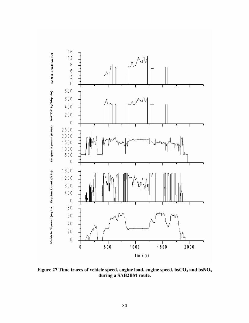
N 0 u ~ .c

:c t 'C ~ 0 ..I ~ ,5 Cl C IIJ

:2 C.

i 'C ~ ~ C. 'II ~

'tl :E ~

1 5 1 2

9 6 3 0

8 0 0

6 0 0

4 0 0

2 0 0

0 2 5 0 0 2 0 0 0 1 5 0 0 1 0 0 0

5 0 0 0

1 6 0 0

1 2 0 0

8 0 0

4 0 0

0 8 0

6 0

4 0

2 0

0

0 500 100 0 1 5 0 0 2000

Time (s)

Figure 27 Time traces of vehicle speed, engine load, engine speed, bsCO2 and bsNOx during a SAB2BM route.

80

On the return journey on the Bruceton Mills route, the average vehicle speed is was 40 mph, with the maximum of approximately 70 mph. The maximum vehicle speed is encountered when the vehicle starts descending the hill from Coopers Rock up to Cheat Lake as shown in Figure 28. The road grade during downhill is 5% as shown in Figure 29.

81

0 z

X

]

-e.:

=-.: J:I

! o" u ]

1 4 1 2 1 0

8 6 4 2 0

7 0 0 6 0 0 5 0 0 4 0 0 3 0 0 2 0 0 1 0 0

0

i 2 5 0 0 C. 2 0 0 0 ~ "C ~ ~

1 5 0 0

: 1000

~ 5 0 0

-~ 0 IIJ

:c 1600 14 0 0

iE. 1200 "C ~ 0 .J ~

.5 Cl : IIJ

1 0 0 0 8 0 0 6 0 0 4 0 0 2 0 0

0

8 0 7 0 6 0 5 0 4 0 3 0 2 0 1 0

0

0 500 100 0 150 0 2000

Time (s)

Figure 28 Time traces of vehicle speed, engine load, engine speed, bsCO2 and bsNOx during a BM2SAB route.

82

1500 Saltwell Exit

1250

1000

g ~ 750

"' ;l:

500

250

0 10 15 20 25 30

Distance (mile)

On the outward journey, except for the starting period from Sabraton test facility to the ramp that connects to I-79, the vehicle speed was approximately 40 mph. The maximum variation in altitude was encountered during the route was about 500 ft over a distance of 5 miles, when the vehicle ascends from an altitude of 750 ft to about 1250 ft as illustrated in Figure 29. The average and maximum vehicle speeds during the route were 50 mph and 70 mph respectively as shown in Figure 30.

Figure 29 Altitude profile for the SAB2SW route

The return journey was very similar to the outbound journey with only very slight changes in average and maximum speed as shown in Figure 31. Also the load factors were similar.

83

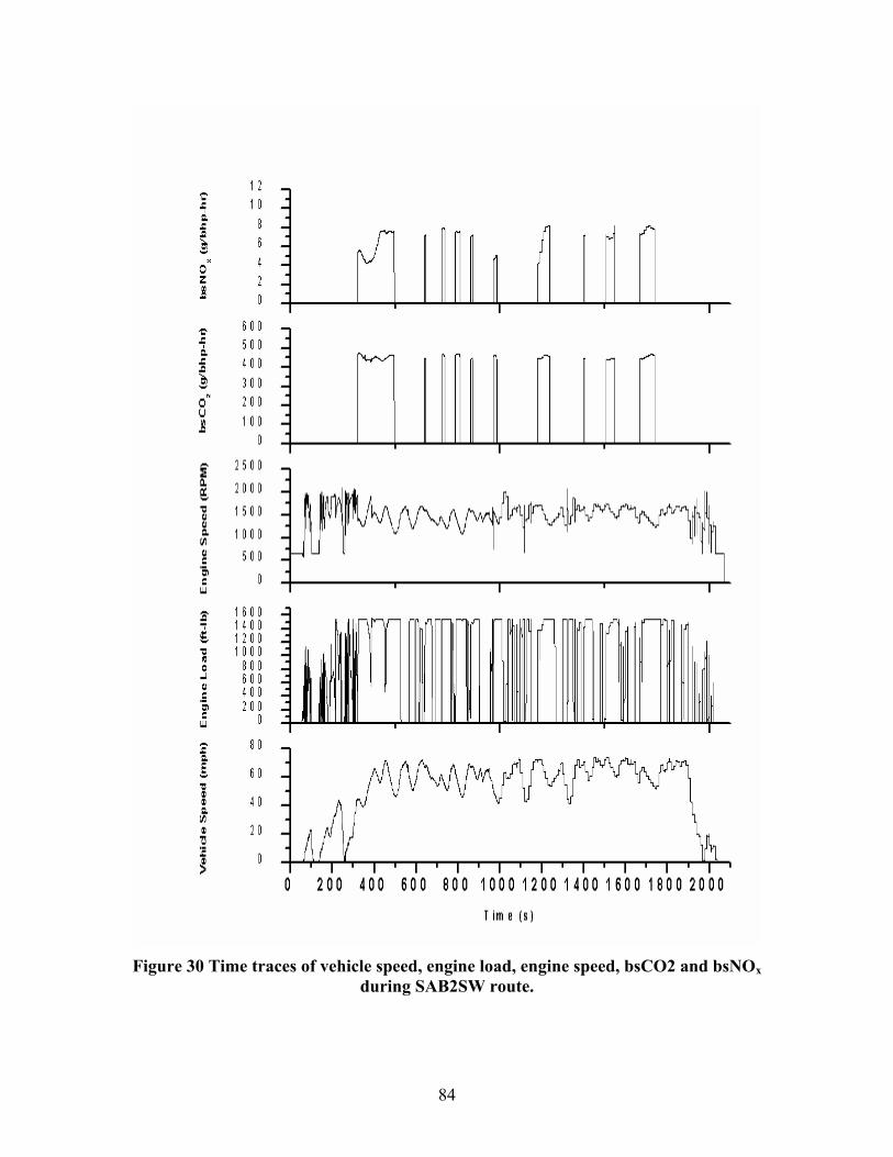
1 2 ,;-

1 0 .:: C.

8 .:: -= s

" 0 z ]

-e- 6 0 0 -.:: 5 0 0 C. .:: 4 0 0 -= s 3 0 0

-~ ..,.

"" --

0 " 2 0 0 u

1 0 0 ]

. --

I I

i 2 5 0 0 Q.

2 0 0 0 ~ -= 1 5 0 0 ~ ~ C. 1 0 0 0 Ill ~ 5 0 0 : ·s,

0 : IIJ

:a 1 6 0 0

i 14 0 0 1 2 0 0

- n,.,...~ - ~ .r J r I' ~! ---= 1 0 0 0 ~

8 0 0 0 .J 6 0 0 ~ 4 0 0 .5 C) 2 0 0

-----: 0 IIJ I I

:2 8 0 C.

i 6 0 -= ~

4 0 ~ C. Ill ~

'O 2 0

:E ~

0 200 400 600 800 1000 1200 1400 1600 1800 2000

Time (s)

Figure 30 Time traces of vehicle speed, engine load, engine speed, bsCO2 and bsNOx during SAB2SW route.

84

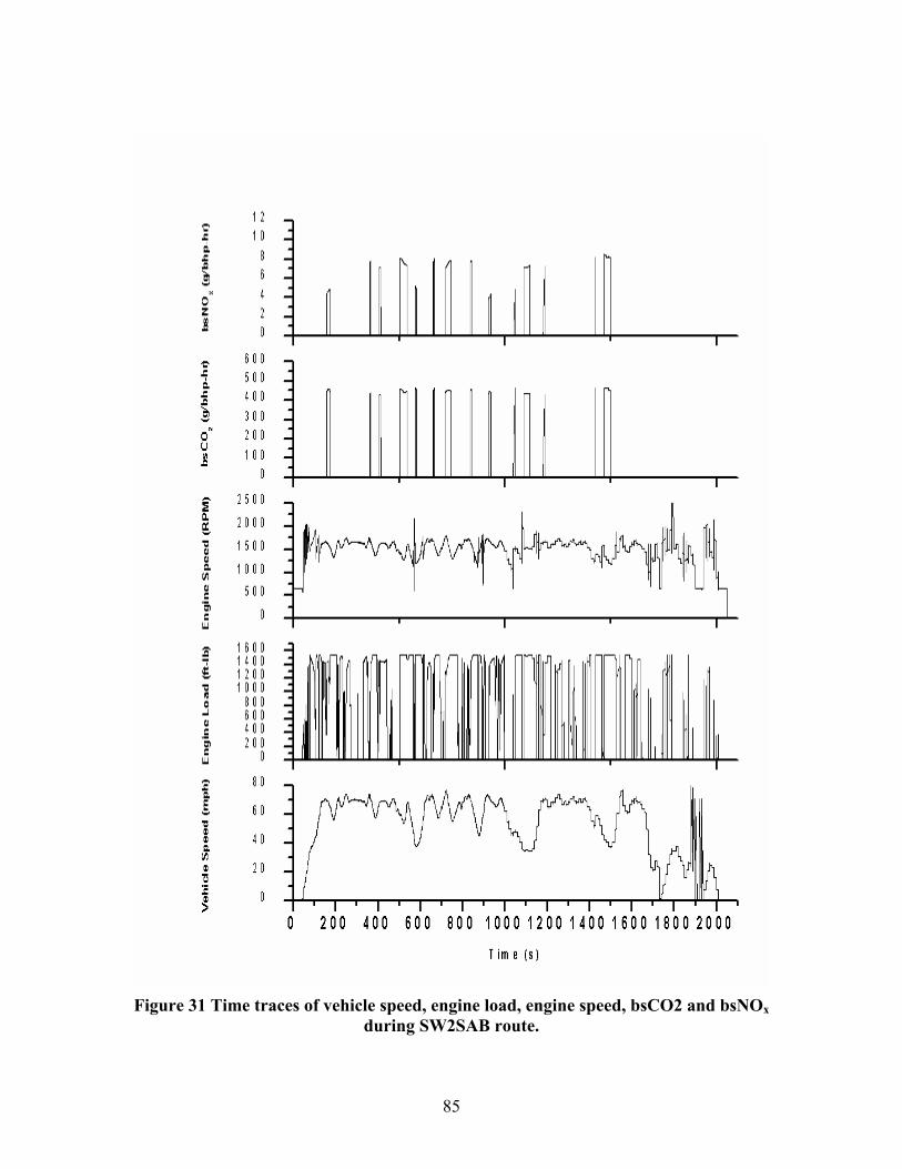
1 2 -~

1 0 .:. C.

8 .:. .c

-- I\

~

I

! -. X

0 z ]

-~

. -

I I

'C' 6 0 0 -.:. 5 0 0 C. .:. 4 0 0 .c ! 3 0 0

-I'- ~

--

0 .

2 0 0 . -u

1 0 0 ] -I I

i 2 5 0 0 C. 2 0 0 0 ~ '!l 15 0 0 ~ ~ C. 1 0 0 0 Ill ~ 5 0 0 : 'ill

0 : U.J

~ 1 6 0 0

t 14 0 0 1 2 0 0

- ~ r rv ,- n J - \ -'!l 1 0 0 0 ~ 8 0 0 0

--.J 6 0 0 ~ 4 0 0 .5 Cl 2 0 0 : 0 U.J

--I II - I

I

:c-C.

8 0

i 6 0 '!l ~

4 0 ~ C. Ill ~ 2 0 '!l :c ~

0 200 400 600 800 1000 1200 1400 1600 1800 2000

Time (s)

Figure 31 Time traces of vehicle speed, engine load, engine speed, bsCO2 and bsNOx during SW2SAB route.

85

12 Uncertainty Analysis

12.1 Introduction

Every measurement is a combination of the true value of the parameter plus the total measurement error. Hence, there is an inherent uncertainty in the use of the measurements to represent a true value. This makes completely accurate measurements impossible. The total uncertainty in a measurement is a combination of uncertainty due to systematic error and uncertainty due to random error. The uncertainty or error analysis is the process of establishing these combined errors.

The analysis presented herein focuses on establishing the uncertainty in measuring brake-specific emissions from portable and stationary engines. As a result of the presentation of the analysis, WVU concluded that flow measurement error was a significant percentage of overall measurement error. Owing to this fact, and to the fact that exhaust flow rate measurement increases system cost, complexity, and limits adaptability, WVU was driven to form recommendations that focused on a concentration ratio-based compliance factor.

12.2 Assumptions

The following are the major assumptions that are made during the measurement uncertainty analysis:

The test process is defined;

The measurement system and test process are controlled;

The appropriate calibration corrections are applied;

The test objectives are specified;

The instrument package and data reduction procedures are defined; and

For purpose of total uncertainty calculations, 95% confidence levels have been used.

12.3 Classification of Measurement Error

The total measurement error consists of two components namely, systematic or bias error and random error.

12.3.1 Random Error

Random error is the portion of the total measurement error that varies in repeated measurements of the true value. The total random error in a measurement is the sum of the contributions of several elemental random error sources. Elemental random errors

86

may arise from non-repeatability in the measurement system, environmental conditions, data reduction techniques and measurement methods.

12.3.2 Systematic Error

Systematic error is the proportion of the total measurement error that remains constant in repeated measurements of the true value. The total bias error in a measurement is the sum of the contributions of several elemental systematic errors. Sources of elemental bias errors are imperfect calibration correction, data acquisition systems, data reduction techniques etc.

12.4 Classification of Components of Uncertainty

The total uncertainty in a measurement is the combination of uncertainty due to systematic error and uncertainty due to random error.

12.4.1 Uncertainty due to Random Error

Random error introduces scatter in repeated measurements of a parameter. The population standard deviation is a measure of the scatter about the true population mean. It is assumed that the random error follows the normal distribution and has been used for the calculation of errors.

12.4.2 Uncertainty due to Bias Error

The uncertainty due to the systematic error cannot be quantified; hence, has to be estimated. The systematic error is an estimate of the systematic error calculated at 95% confidence.

12.5 Classification of Type of Uncertainty evaluation

The uncertainty is evaluated by two methods-Type A and Type B.

12.5.1 Type A Evaluation

The evaluation of uncertainty by the statistical analysis of series of observations is termed as Type A evaluation of uncertainty.

12.5.2 Type B Evaluation

The evaluation of uncertainty by means other than the statistical analysis of series of observations is termed as Type B evaluation of uncertainty.

87

12.6 Measurement Uncertainty Sources

Uncertainty in a measurement process may be introduced from the following sources: calibration, data acquisition, data reduction, and methods.

12.6.1 Calibration Uncertainty

Calibration is the process of feeding known input values into the measurement system and recording the output to use as a reference when reducing data. The main purpose of calibration process is to eliminate large, known systematic errors and thus reduce the measurement uncertainty to some acceptable level.

12.6.2 Data Acquisition Uncertainty

Uncertainty in data acquisition systems can arise from errors in the signal conditioning, the sensors, the recording devices etc. Overall system calibration reduces the effects of these uncertainty sources. The overall uncertainty is evaluated by combining each of the elemental uncertainties.

12.6.3 Data Reduction Uncertainty

Mostly the data is presented in engineering units. Converting the raw data by performing necessary computations does this. Typical uncertainty sources arise from curve fit errors and the computational resolution.

12.6.4 Uncertainty due to Methods

Uncertainties due to methods are defined as those additional uncertainty sources that originate from the techniques or methods inherent in the measurement system. Some of them include:

Uncertainty in the assumptions or constants contained in the calculation routines;

Uncertainty due to intrusive disturbance effects caused by installed instrumentation;

Environmental effects on probes such as heat transfer effects;

Uncertainty due to instability, non-repeatability, and hysteresis of the test process.

The uncertainties may be of either random or bias nature depending on their effect on the measurement.

12.7 Propagation of Uncertainty

The objective of the error model is to assess the contribution of individual measurement uncertainties to the final result. The procedures have been described in National Institute of Standards for the purpose. They are

88

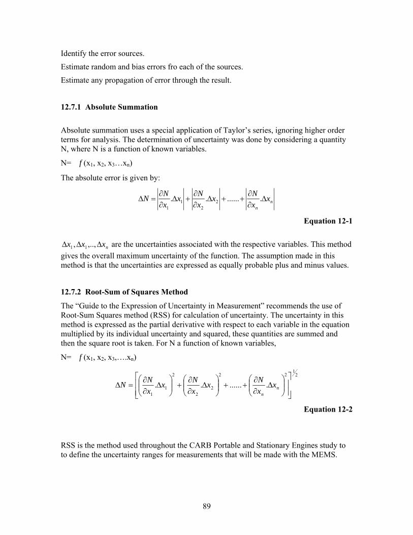
I

Identify the error sources.

Estimate random and bias errors fro each of the sources.

Estimate any propagation of error through the result.

12.7.1 Absolute Summation

Absolute summation uses a special application of Taylor’s series, ignoring higher order terms for analysis. The determination of uncertainty was done by considering a quantity N, where N is a function of known variables.

N= f (x1, x2, x3…xn)

The absolute error is given by:

∂N ∂N ∂N∆N = .∆x1 + .∆x2 + ......+ .∆xn∂x1 ∂x2 ∂xn

Equation 12-1

∆x1 , ∆x1 ,.., ∆xn are the uncertainties associated with the respective variables. This method gives the overall maximum uncertainty of the function. The assumption made in this method is that the uncertainties are expressed as equally probable plus and minus values.

12.7.2 Root-Sum of Squares Method

The “Guide to the Expression of Uncertainty in Measurement” recommends the use of Root-Sum Squares method (RSS) for calculation of uncertainty. The uncertainty in this method is expressed as the partial derivative with respect to each variable in the equation multiplied by its individual uncertainty and squared, these quantities are summed and then the square root is taken. For N a function of known variables,

N= f (x1, x2, x3,….xn)

⎡⎛ ∂N ⎞2

⎛ ∂N ⎞2

⎛ ∂N ⎞2 ⎤

∆N = ⎢⎜⎜ .∆x ⎟⎟ + ⎜⎜ .∆x ⎟⎟ + ...... + ⎜⎜ .∆x ⎟⎟ ⎥1 2 n⎢ ∂x ∂x ∂x ⎥⎣⎝ 1 ⎠ ⎝ 2 ⎠ ⎝ n ⎠ ⎦

Equation 12-2

RSS is the method used throughout the CARB Portable and Stationary Engines study to to define the uncertainty ranges for measurements that will be made with the MEMS.

21

89

I

I

⎟

⎟

⎜

⎜

12.8 Uncertainty in Brake Specific Emissions

To determine the uncertainty in the measurement of brake specific emissions of NOx and CO2, the following equations were used.

NOx) ppm *Qs * * t 106 ρ

bsNOx bhp

Equation 12-3

∂

∂

CO2 ) ppm *Q * * tρ6 s10

∂

Equation 12-4

∂

where,

bsNOx= brake specific emissions of NOx in g/bhp-hr

CO2)ppm= concentration of carbon dioxide in ppm Qs= exhaust flow rate in scfm

= brake specific emissions of CO in g/bhp-hrbsCO2 2 ) = concentration of oxides of nitrogen in ppmNOx ppm

bhp-hr= work done or energy

∂

ρ= density of the gas in lb/ft3

t= time in seconds Using the Root-Mean Square method, and assuming the density to be a constant, the uncertainty in the brake specific emissions may be expressed as:

12

bsNOx bsNOx bsNOx ⎜ ⎟Q bhp

⎛ ⎞⎟ ⎟ ⎟ ⎟

bsCO2 bhp ⎠

2 ⎤2 ⎞⎟ ⎠ ⎥ ⎥⎦

bsNO NOx Q bhp∆ .∆ .∆+ +.∆x sNOx s

Equation 12-5

1222 ⎤

∂

∂

∂

∂

∂

∂bsCO bsCO bsCO2 2 2 ⎟ ⎜ ⎟CO Q bhp

Equation 12-6

where,

90

⎞⎟ ⎠ ⎥ ⎥⎦

bsCO CO Q bhp∆ + +.∆ .∆ .∆2 2 s ⎛⎜ ⎝ ⎢ ⎢⎣ ⎜

2 s

⎞⎟ ⎟ ⎟⎟

⎛

⎠

⎜ ⎜ ⎜⎜⎝

=

⎜ ⎜ ⎜ ⎜⎝

=

⎛⎜ ⎝

⎞⎟ ⎠

⎛⎜ ⎝

⎞⎟⎠

⎛⎜⎝ ∂

⎡ ⎢ ⎢⎣

=

⎛⎜ ⎝

⎞⎟ ⎠

⎛⎜ ⎝

⎞⎟ ⎠

⎡ =

2

I

∆bsNOx= uncertainty in the bsNOx measurement ∆bsCO2= uncertainty in the bsCO2 measurement

∆Qs= uncertainty in the exhaust flow rate measurement ∆bhp-hr= uncertainty in the energy measurement

The first variability considered in the brake specific emissions measurements was the exhaust flow rate. The exhaust flowrate was measured using the Annubar. To determine the uncertainty in the exhaust flow rate, the following equation was used.

2 14.696Q = F *K *D *F *Y *F *F *F *F *F *F *F *F * h * s NA RA A pb tb tf s pv m AA l w 29.92

Equation 12-7 where,

D= Internal Diameter of pipe, inches FAA= Thermal Expansion Factor.

Fg= Specific Gravity Factor. (Assumed constant) Fl= Gage Location Factor. (Assumed constant) Fm= Manometer Factor. (Assumed constant)

FNA= Units Conversion Factor. (Assumed constant) Fpb= Pressure Base Factor. (Assumed constant)

Fpv= Supercompressibility Factor. (Assumed constant) FRA= Reynolds Number Factor. (Assumed constant) Ftb= Temperature Base Factor. (Assumed constant)

Ftf= Flowing Temperature Factor. hw= Differential pressure as measured by the Annubar primary element.

K= Flow Coefficient. Pf= Flowing Pressure. YA= Expansion Factor.

The error associated with the total mass flow rate was calculated as follows. 1

⎡ 2 2 ⎤2 2 2 2 ⎛ ∂Q ⎞ ⎛ ∂Q ⎞ ⎛ ∂Q ⎞ ⎛ ∂Q ⎞ ⎛ ∂Q ⎞ ⎛ ∂Q ⎞

s s s s s∆Qs = ⎢⎜ * ∆K ⎟ + ⎜⎜ * ∆YA ⎟⎟ + ⎜⎜ * ∆FAA ⎟⎟ + ⎜ * ∆Ftf ⎟ + ⎜⎜ * ∆hw ⎟⎟ + ⎜ * ∆Pf

⎟ ⎥⎜ ⎟ ⎜ ⎟⎢⎝ ∂K ⎠ ⎝ ∂YA ⎠ ⎝ ∂FAA ⎠ ⎝ ∂Ftf ⎠ ⎝ ∂hw ⎠ ⎝ ∂Pf ⎠ ⎥

⎣ ⎦

Equation 12-8

The Flow Coefficient K was determined by calibrating the Annubar against the LFE. The uncertainty in the K value was determined as follows.

91

/ 1 ⎡ 2 2 2 ⎤ 2 ⎛ ∂K ⎞ ⎛ ∂K ⎞ ⎛ ∂K ⎞'∆K = ⎢⎜⎜ ' .∆ Q ⎟⎟ + ⎜⎜ .∆ h w ⎟⎟ + ⎜ .∆ P f

⎟ ⎥⎜ ⎟⎢ ∂Q ∂h ∂P ⎥⎝ ⎠ ⎝ w ⎠ ⎝ f ⎠⎣ ⎦

Equation 12-9

where,

Q ' = volumetric flow rate through the LFE in scfm. The flow rate was measured with a Laminar Flow Element (LFE) using the following equation.

Q ' = (B * DP + C * DP 2 )* ⎛⎜ µ std

⎞⎟ *⎜⎛

Tstd ⎟⎞ *⎜⎜

⎛ Pf ⎟⎟⎞

⎜ ⎟⎝ µ f ⎠ ⎝ T ⎠ ⎝ Pstd ⎠

Equation 12-10

where,

B and C = calibration constants for the LFE. DP = differential pressure across the LFE in inches of water.

µ std = viscosity of flowing gas at 70 F in micropoise. µ f = viscosity of flowing gas at flowing temperature in micropoise.

Tstd = standard temperature in Fahrenheit. Tf = flowing gas temperature in Fahrenheit.

Pstd = standard pressure in inches of mercury. Pf = flowing pressure in inches of mercury.

The uncertainty in the flow rate measured using the LFE is given by:

'∆Q = 2⎡ '⎛ ∂Q ⎞⎢⎜⎜ ∆. DP⎟⎟ ⎢ ∂DP⎝ ⎠⎣

'⎛ ∂Q+ ⎜⎜ ∂T⎝

2⎞

∆. T ⎟⎟ ⎠

'⎛ ∂Q+ ⎜⎜ ∂P⎝ f

∆. Pf

2 ⎤⎞⎟ ⎥⎟ ⎥⎠ ⎦

Equation 12-11

where,

∆DP = uncertainty in the differential pressure measurement. ∆T = uncertainty in the temperature measurement.

∆Pf = uncertainty in the absolute pressure measurement.

92

I I

I I

The LFE absolute pressure and the differential pressure were measured using a Digital calibrator type Heise PTE-1.The total error in each of the measurement is listed in Table 19.

The LFE inlet temperature was measured with a Fluke 714 Thermocouple Calibrator. The total error in the measurement of temperature is listed in Table 19.

Table 19 List of instruments used for differential & absolute pressure and temperature measurement

Parameter Manufacturer Model Accuracy

Differential Pressure Heise HQS-1 ± 0.06% of Span

Absolute Pressure Heise HQS-2 ± 0.025% of Span

Temperature Fluke 714 Thermocouple Calibrator

± 0.025% of Reading

The Annubar absolute pressure was measured using a Omega PX-213 pressure transducer. The total error in the measurement is listed in Table 20.

Table 20 Errors in absolute pressure measurement

Source Manufacturer Model Number Applied Error % of Full Scale

Absolute Pressure Sensor Omega Inc. PX213 ±0.25%

Signal Conditioner Module

National Instruments Inc. SCC-AI04 ±0.1%

DAQ Board National Instruments Inc. NI-6024E ±0.0244%

The Annubar differential pressure was measured with a Validyne P55D differential pressure transducer. The total error in the measurement is listed in Table 21.

93

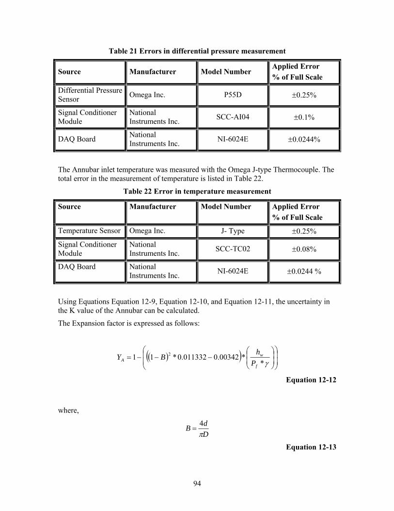
I I I I

Table 21 Errors in differential pressure measurement


Differential Pressure Sensor Omega Inc. P55D ±0.25%


National Instruments Inc. SCC-AI04 ±0.1%

DAQ Board National Instruments Inc. NI-6024E ±0.0244%

The Annubar inlet temperature was measured with the Omega J-type Thermocouple. The total error in the measurement of temperature is listed in Table 22.

Table 22 Error in temperature measurement


Temperature Sensor Omega Inc. J- Type ±0.25%


National Instruments Inc. SCC-TC02 ±0.08%

DAQ Board National Instruments Inc. NI-6024E ±0.0244 %

Using Equations Equation 12-9, Equation 12-10, and Equation 12-11, the uncertainty in the K value of the Annubar can be calculated.

The Expansion factor is expressed as follows:

YA

⎛⎜= 1− (( 1−⎜⎝

2B) ⎛

* 0.011332 − )0.00342 *⎜⎜⎝

hw

P *γf

⎞⎞⎟⎟ ⎟⎟⎠⎠

Equation 12-12

where,

B = 4d Dπ

Equation 12-13

94

I

I ⎜ ⎟

B= Blockage D= Internal pipe diameter

d =0.173 for shape 10 =0.365 for shape 15/16 =0.856 for shape 25/26

hw= Differential pressure as measured by the Annubar primary element. Pf= Flowing pressure.

γ = Ratio of specific heats. The ratio of specific heats is expressed as:

5 4 3γ = −3.34642E −16*(T + 273) + 9.26157E −14(T + 273) − 7.64644E −10*(T + 273) + 6.48889E − 8*(T + 273)2 + 0.0000514974*(T + 273) +1.3927

Equation 12-14

The error in the value of ratio of specific heats is given by:

⎡ 2 ⎤⎛ ∂γ ⎞∆γ = ⎢⎜ .∆T ⎟ ⎥ ⎢⎝ ∂T ⎠ ⎥⎣ ⎦

Equation 12-15

From this the uncertainty in the expansion factor is calculated as :

∆YA

2⎡⎛ ∂Y ⎞A= ⎢⎜⎜ .∆hw ⎟⎟ ⎢ ∂h⎝ w ⎠⎣

⎛ ∂YA+ ⎜ .∆Pf⎜ ∂P⎝ f

2⎞⎟⎟⎠

2 ⎤⎛ ∂Y ⎞A+ ⎜ .∆γ ⎟ ⎥ ∂γ ⎥⎝ ⎠ ⎦

Equation 12-16

The uncertainty in the Annubar absolute pressure, Annubar differential pressure, thermal expansion factor, temperature base factor, and flowing temperature factor can be calculated using Equation 12-17 through Equation 12-20.

∂Qs Qs= ∂F Ftf tf

Equation 12-17

21

21

95

∂Qs Qs= ∂F FAA AA

Equation 12-18

Q∂ s = Qs

h∂ w 2hw

Equation 12-19

∂Qs Qs= ∂Pf 2Pf

Equation 12-20

Inserting the values from Equation 12-9, Equation 12-16 through Equation 12-20, and the values of ∆hw, ∆Pf and ∆T into Equation 12-8 gives the value of the uncertainty in the exhaust flow rate measurement (∆Qs).

12.9 Calculating the Uncertainty of Concentration Values

12.9.1 Calibration Error

The error from the gas analyzer calibration is associated with the uncertainties in the reported calibration gas concentration, the gas divider, the signal conditioner and the conversion of ADC codes to engineering unit values. The manufacturer-supplied values of accuracies of each of them are given the Table 23.

Table 23 Specifications of instruments used in gaseous concentration measurement

Source Manufacturer Model No. Applied Error Calibration Gas Scott Specialty Gases N/A ± 1.0 % Gas Divider STEC Inc. SGD- 710C ± 0.54 % Signal Conditioner National Instruments SCC- AI-04 ± 0.1 % DAQ- Board National Instruments 6024-E ± 0.0244 %

2 2 2 2Rcal = 1.0 + 0.54 + 0.1 + 0.0244 = ±1.14% full scale

Equation 12-21

96

12.9.2 Data Reduction Error

The uncertainty introduced in the data reduction process is from the goodness of fit of the models used from the calibration curves.

Curvefiterror = (yreal

2− y )curvefit

v * tv,95

Equation 12-22

where,

v= n-p+1 n = number of data points summed.

p=order of the fit equation. tv, 95= student t- distribution

12.9.3 Analyzer Error

Table 24 Specifications of gas analyzers used

Analyzer Manufacturer Model % Error

CO2 Horiba Inc. BE-140 ± 2% of Full Scale reading

NOx Horiba Inc. MEXA-120 ± 30 ppm <1000ppm

± 3% reading for 1000-2000 ppm

The total error in the measurement of NOx concentrations is given by 2 2 2∆NO ) = Analyzer _ Error + Calibration _ Error + Curvefit _ Errorx ppm

Equation 12-23

12.9.4 Power or Energy Error

The energy is calculated by integrating the brake horsepower over time. The brake horse power is calculated as follows:

bhp − hr = (torque * rpm)* 2π 550 *60

Equation 12-24

97

_t

⎟ ⎜ ⎟ ⎜

Therefore the equation that determines the error in the calculation of energy is:

⎛∂bhp − hr ⎞2

⎛∂bhp − hr ⎞2

∆bhp − hr =⎜ .∆torque⎟ +⎜ .∆rpm⎟ ⎝∂torque ⎠ ⎝∂rpm ⎠

Equation 12-25

where,

∆torque = the error associated with the torque measurements ∆rpm = the error associated with engine speed measurements

By substituting Equation 12-23 through Equation 12-25 and Equation 12-8 into Equation 12-5 and Equation 12-6, the uncertainty in the brake specific emissions of NOx and CO2 may be calculated.

The following section provides an estimate of the uncertainty in the NOx concentrations measured by zirconium oxide sensor, CO2 concentrations, measured by the BE-140 system, and PM concentrations measured by the CVS and the Method 5 systems.

According to Horiba Inc., the zirconium oxide sensor for NOx has a bias error of ± 30 ppm for concentrations less than 1000 ppm. The bias error is ± 3 % for concentrations above 1000 ppm. The total uncertainty in Zirconium Oxide NOx sensor concentration (including both bias and random errors) is 30.4 (<1000 ppm) and ± 3.36 % of the value, for values above 1000 ppm [64]. The Horiba BE-140 sensor has a bias error of ± 2% of full scale. The total uncertainty for CO2 concentrations measured by the BE-140 sensor has been estimated to be 2.3 % full scale [64]. PM concentrations measured by the CVS method are estimated to have a total uncertainty of 1.95% [65]. The manufacturer reported bias for Method 5 PM sampling system is 6%. The total uncertainty in PM mass measurement from Method 5 system is estimated using the student’s t distribution,

t × STDEV α /2, n−1Randomerror =

n

where tα/2, n-1 represents the student t value for 95% confidence, with (n-1) degrees of freedom. STDEV is the standard deviation of a set of repetitive values from the mean, and n is the number of repeats or runs. Since there were three runs for every Method 5 test mode, n is equal to 3, resulting in a t value of t0.025, 3 = 4.303

The total uncertainty was calculated using the relation,

U95 = 2 2

) ( ) ( error random Bias +

Total uncertainty associated with modified Method 5 could not be performed due to the absence of information on bias errors. Also, the limited number of runs using the modified method 5 system made it difficult to do a statistical analysis of random error.

98

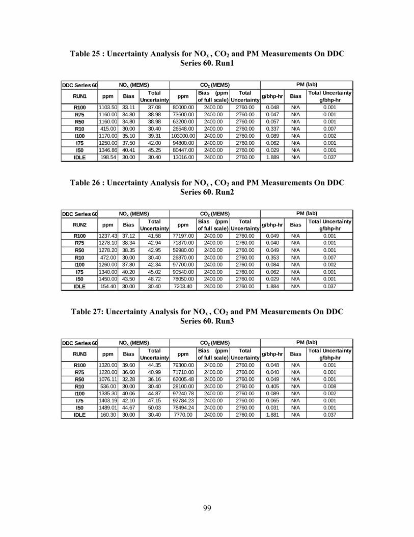
Table 25 : Uncertainty Analysis for NOx , CO2 and PM Measurements On DDC Series 60. Run1

DDC Series 60 NOx (MEMS) CO2 (MEMS) PM (lab)

RUN1 ppm Bias Total Uncertainty

ppm Bias (ppm of full scale)

Total Uncertainty

g/bhp-hr Bias Total Uncertainty g/bhp-hr

R100 1103.50 33.11 37.08 80000.00 2400.00 2760.00 0.048 N/A 0.001 R75 1160.00 34.80 38.98 73600.00 2400.00 2760.00 0.047 N/A 0.001 R50 1160.00 34.80 38.98 63200.00 2400.00 2760.00 0.057 N/A 0.001 R10 415.00 30.00 30.40 26548.00 2400.00 2760.00 0.337 N/A 0.007 I100 1170.00 35.10 39.31 103000.00 2400.00 2760.00 0.089 N/A 0.002 I75 1250.00 37.50 42.00 94800.00 2400.00 2760.00 0.062 N/A 0.001 I50 1346.86 40.41 45.25 80447.00 2400.00 2760.00 0.029 N/A 0.001

IDLE 198.54 30.00 30.40 13016.00 2400.00 2760.00 1.889 N/A 0.037

Table 26 : Uncertainty Analysis for NOx , CO2 and PM Measurements On DDC Series 60. Run2


RUN2 ppm Bias Total Uncertainty ppm Bias (ppm

of full scale) Total

Uncertainty g/bhp-hr Bias Total Uncertainty g/bhp-hr


IDLE 154.40 30.00 30.40 7203.40 2400.00 2760.00 1.884 N/A 0.037

Table 27: Uncertainty Analysis for NOx , CO2 and PM Measurements On DDC Series 60. Run3






IDLE 160.30 30.00 30.40 7770.00 2400.00 2760.00 1.881 N/A 0.037

99

Table 28 : Uncertainty Analysis for NOx , CO2 and PM Measurements On Isuzu C 240. Run1

ISUZU C 240 NOx (MEMS) CO2 (MEMS)

RUN1 ppm Bia s Tota l Uncerta inty

ppm Bia s (ppm of full sca le )

Tota l Uncerta inty

R100 437.56 30.00 30.40 103634.02 2400.00 2760.00 R75 368.87 30.00 30.40 76552.85 2400.00 2760.00 R50 257.37 30.00 30.40 57377.76 2400.00 2760.00 R10 95.90 30.00 30.40 30877.20 2400.00 2760.00 I100 303.26 30.00 30.40 106837.17 2400.00 2760.00 I75 383.44 30.00 30.40 80523.15 2400.00 2760.00 I50 383.27 30.00 30.40 57806.85 2400.00 2760.00

IDLE 16.47 30.00 30.40 2388.96 2400.00 2760.00


ISUZU C 240 NOx (MEMS) CO2 (MEMS) PM (lab)





IDLE 15.67 30.00 30.40 2011.80 2400.00 2760.00 0.240 N/A 0.005







IDLE 16.73 30.00 30.40 2050.56 2400.00 2760.00 0.310 N/A 0.006

100







IDLE 16.28 30.00 30.40 2162.32 2400.00 2760.00 0.290 N/A 0.006 Zirconium Oxide NOx sensor bias from Horiba Inc., = ± 30 ppm < 1000 ppm and ± 3% reading for 1000-2000 ppm.

Table 32 : Uncertainty Analysis for PM Measurements Using Method 5 System On Isuzu C 240.

ISUZU C 240 PM (M5) W/O BHE PM (M5) With BHE

RUN1 g/bhp-hr Bias Total Uncertainty g/bhp-hr


R100 0.119 0.007 0.019 0.205 0.012 0.037 I100 0.149 0.009 0.014 0.235 0.014 0.055

ISUZU C 240 PM (M5) PM (M5)

RUN2 g/bhp-hr Bias Total Uncertainty g/bhp-hr


R100 0.130 0.008 0.019 0.232 0.014 0.037 I100 0.158 0.009 0.015 0.228 0.014 0.055

ISUZU C 240 PM (M5) PM (M5)

RUN3 g/bhp-hr Bias Total Uncertainty g/bhp-hr g/bhp-hr Bias Total Uncertainty

g/bhp-hr

R100 0.132 0.008 0.019 0.225 0.014 0.037 I100 0.154 0.009 0.015 0.268 0.016 0.055

101

Table 33: Uncertainty Analysis for PM Measurements Using Method 5 System On DDC Series 60.

DDC SERIES 60 PM (M5) W/O BHE PM (M5) With BHE


g/bhp-hr I75 0.056 0.003 0.004 0.075 0.005 0.006 I50 0.040 0.002 0.016 0.086 0.005 0.055

DDC SERIES 60 PM (M5) PM (M5)


g/bhp-hr I75 0.058 0.003 0.005 0.072 0.004 0.006 I50 0.040 0.002 0.016 0.084 0.005 0.055

DDC SERIES 60 PM (M5) PM (M5)


g/bhp-hr

I75 0.056 0.003 0.004 0.075 0.005 0.006 I50 0.029 0.002 0.016 0.047 0.003 0.055

The uncertainty associated with PM measurements using the mini-dilution tunnel is shown below. Total uncertainty associated with mini-dilution tunnel based PM measurements is a function of engine speed and the load on the engine [66] and varies between 2.8 % to 10% of the reading. A mean value of 6.4% total uncertainty was chosen for the following analyses.

Table 34 : Uncertainty Analysis for PM Measurements Using Mini-Dilution System On DDC Series 60.

DDC Series 60

PM (Mini-tunnel ) g/bhp-hr Bias Total Uncertainty

R100-1 0.05027

N/A

0.0032 R100-2 0.03443 0.0022 R100-3 0.03923 0.0025 R100-4 0.04386 0.0028 R100-5 0.03587 0.0023 R100-6 0.03875 0.0025 R100-7 0.03918 0.0025

I50 0.02725 0.0017 R75 0.03689 0.0024 R100 0.0343 0.0022 I50 0.027184 0.0017 R75 0.03223 0.0021

102

12.10 Results and Discussions on Uncertainty in Brake-Specific Emissions

The flow measurement system employed in MEMS involved measuring several parameters namely absolute pressure, differential pressure, and temperature. Equation 1.6 gives the error associated with the total exhaust mass flow rate. The uncertainty in bsNOx increases almost linearly with an increase in the total error in the measurement of NOx concentration values. The analysis was applied to an on-road tractor operation, and the uncertainty in the brake-specific emissions of NOx and CO2 in the not-to-exceed zone, using the MEMS was found to be less than 10% and less than 8%, respectively. The analyzers, the exhaust flow rate, pressure transducers, temperature sensors, thermocouples, the flow constant for the Annubar, K were all considered as sources of error in the uncertainty calculations. A sensitivity analysis on the brake-specific emissions measurements, revealed the sources of uncertainty. It was found that exhaust flow uncertainty, a function of errors in measurement of absolute pressure, differential pressure, Annubar flow coefficient goes up to 12%. It can be inferred that the exhaust flow measurement is the major source of uncertainty in the calculation of brake-specific emissions.

103

13 Results & Discussion:

The objective of this study was to develop a cost-effective in-the-field test method for stationary and portable engines that would be used to determine compliance with emission standards for newly manufactured off-road engines. The test method and protocols developed in this study will allow determination of engine compliance with emission limits established by the Statewide Portable Equipment Registration Program. The method has been shown to accurate, cost-effective, and reliable and it allows for quantification of fuel-specific mass emissions from both, diesel- and gasoline-fueled portable and stationary engines under real-world conditions. Measurement tools discussed in this report and some of the commercially available tools could be employed for determination of brake-specific emissions.

WVU has developed an in-the-field cost-effective test method for stationary and portable engines that is capable of determining compliance with emissions standards for newly manufactured off-road engines as promulgated by either the California Air Resources Board (CARB) or the U.S. Environmental Protection Agency (EPA). Recognizing the fact that most stationary and portable engines are mechanically controlled, that is, they do not have any means of broadcasting engine speed and load, the commercially available portable emissions measuring instruments are not equipped to provide brake-specific emissions data from such engines. As stated earlier, determination of mass emissions would involve measurement of exhaust flow rate, which is one of the biggest sources of uncertainty in in-use emissions measurements. Unfortunately, most stationary and portable engines in the field will not allow ready access to the engine stack for measurement of exhaust flow rates.

Constraints that challenged the design and development of an in-field test method for stationary and portable engines were discussed in the Introduction chapter.

Discussed below is data that was generated in the process of evaluating various tools for measuring regulated emissions, conclusions that were drawn from these results, and the development and validation of the “Compliance Factor” approach that is being recommended to CARB as a means of determining compliance of engines in the field.

Given all the limitations, complexities, and uncertainties associated with measuring brake-specific measurements from stationary and portable engines, WVU is recommending a method that uses concentration measurements only, and the equipment necessary to conduct such measurements would be very inexpensive; hence, easily affordable.

Before discussing the results of sensor evaluations, and details of method development, a discussion on the “Compliance Factor” is presented below

13.1 Compliance Factor

The following section provides a basis for the discussion of the compliance factor, F. The section illustrates the application of this methodology to obtain estimates for compliance factor F, using the data gathered from two engines that were exercised on multiple ISO

104

I I

8178 certification test cycles. The test method thus developed, was then applied to two other engines operated on their regular duty cycle (in-use operation) to obtain the values for the compliance factor F during such in-use operation of engines. Using this information it may be possible to simplify the current compliance monitoring procedure for newly manufactured off-road engines.

Let r1 be the ratio of the mass of NOx over mass of CO2. Let r2 be the ratio of mass of NOx over mass of fuel consumed. Hence, r1 is the CO2-specific ratio and r2 the fuel specific ratio.

NOX mass r = 1 CO2 mass

Equation 13-1 Expanding, using the definition of Mass,

Mass = Density x Volume

Equation 13-2

r1

C ×( MW NOx NOx= C ×( MW CO2 CO 2

c.f)×Volume c.f)×Volume

Equation 13-3

Where C NO is the concentration of NOx in ppm, & C

CO2 is the concentration of CO2 in

x

ppm. c.f is the conversion factor that relates molecular weight to density. MWNO is the x

molecular weight of NOx and MWCO2 is the molecular weight of CO2. Volume occupied

by the gas is measured in scf (standard cubic feet).

Canceling common terms in the numerator and denominator, yields,

C ×MW NO NO r = x x 1 C ×MW CO CO 2 2

Equation 13-4

105

NOx mass r2 = fuel mass

Equation 13-5

NOx mass r2 = Massof C + Mass of H

Equation 13-6

The following relation is utilized to calculate the mass of carbon, Gs.

12.011 12.011Gs = R2 ×HC mass + ( )× CO mass + ( )× CO2 mass 28.011 44.011

Equation 13-7

Where,

Gs = Grams of carbon measured during operation cycle. HC mass = Grams of hydrocarbon emissions measured during operation cycle.

CO mass = Grams of carbon monoxide emissions measured during operation cycle. R2 = Grams of carbon in the fuel per gram of fuel.

Neglecting the contributions of HC & CO results in:

12.011Gs = Massof C = ( )×CO2 mass 44.011

Equation 13-8

Continuing, to calculate mass of H, the following relationship is used:

Mass = (Molecular weight × Number of moles)

Equation 13-9

Mass of H = 1.008 × (Number of moles of H).

Equation 13-10

The H/C ratio (α) of the fuel (expressed in moles of H per mole of C) is known and if the total number of moles of C is also known, then the total number of moles of H can be determined. Therefore,

106

I

Mass of H =1.008× α( moles H / moleC)×Moles C

Equation 13-11

Where, α=H/C ratio of the fuel, expressed in moles H/mole C. However,

Mass of C Moles C = MWC

Equation 13-12

12.011 44.011×(C

CO2 × )×Volume Mass C 44.011 c.f =

MWC 12.011

Equation 13-13

Canceling common terms,

Mass C CCO2Moles C = = ×Volume MWC c.f

Equation 13-14

CCO2∴Mass of H =1.008 × α × ×Volume c.f

Equation 13-15

Substituting the values for mass of NOx, mass of C & mass of H in the equation for r2,

C ×( MW c.f )×Volume NO NO r = x x 2 C12.011 CO2( )×CO2 mass +1.008×α× ( )×Volume

44.011 c.f Equation 13-16

Again CO2 mass can now be in turn expressed as,

107

I

MWCOCO mass =C × 2 ×Volume 2 CO2 c.f Equation 13-17

Hence, r2 may be rewritten as

CNO ×( MWNO c.f )×Volume r = x x 2

12.011 MWCO2 CCO2( )×CCO × ×Volume +1.008×α× ( )×Volume

244.011 c.f c.f Equation 13-18

Canceling common terms, yields

C ×MW NO NO r = x x 2 12.011×C +1.008×α×CCO CO2 2

Equation 13-19

that is,

C ×MW NO NO r = x x 2 (12.011+1.008×α )×C

CO2

Equation 13-20

rConsidering the ratio 2 , r1

CNO ×MWNOx x

r (12.011+1.008×α )×CCO2 = 2

r1 CNO ×MWNO

x x

C ×MW CO CO2 2

Equation 13-21

r MW2 CO2= r1 12.011+1.008×α

Equation 13-22

108

Assuming an α of 1.85 and MWCO2

as 44.011,

r2 44.011 = = 3.1717

r1 12.011+1.008×1.85

Equation 13-23

The CO2-specific ratio, r1, may be used to represent a ratio of brake specific mass emissions of the pollutants, and is essentially a ratio of pollutant concentrations. The fuel specific ratio, r2, represents ratio of the mass of NOx emitted per mass of fuel consumed and can be calculated using only pollutant concentrations. The value 3.1717, can be applied to obtain these ratios interchangeably, that is, if the ratio r1 given, then the ratio r2 can be estimated and vice versa. This will be useful if we need to convert the manufacturer reported CO2-specific Certification Ratio, C (ratio of brake specific mass emissions of NOx and CO2) to fuel specific Certification Ratio, C (ratio of NOx mass emissions to mass of fuel consumed).

The following tables provide an illustration of the methodology of the test method. A compliance factor, F, is defined as the ratio of In-field Pollutant Ratio (I) and Certification Ratio (C). The In-field Pollutant Ratio is defined as the ratio of mass emissions of NOx to the mass emissions of CO2, for each in-field operation (or each steady state operation mode, as in the case of an ISO 8178 test cycle). The Certification Ratio (C) is defined as the ratio of brake specific NOx (weighted) mass emissions to brake specific CO2 (weighted) mass emissions, each measured over an entire 8-mode cycle. Hence, C is obtained either from the laboratory evaluation of the engine on the ISO 8178 test cycle or using emissions data from the manufacturer. Hence,

IF= C

Equation 13-24

I = (NOx mass emissions)In−field operation

(CO2 mass emissions)In−field operation

Equation 13-25

C = (NOx mass emissions)ISO 8178 test cycle

(CO2mass emissions)ISO 8178 test cycle

Equation 13-26

The reason for expressing the Certification Ratio, C, as a ratio of brake specific emissions is the difficulty associated in getting concentration specific data from the manufacturer. However, the In-field Pollutant Ratio, I, obtained using either r1 (CO2-specific ratio) or r2

109

https://12.011+1.0081.85

(fuel specific ratio), will be determined using only “in-field”concentration data of NOx and CO2. Concentration data is more reliable than brake specific data due to errors associated in exhaust flow rate and work output measurements. However, if the Certification Ratio, C, is needed as a ratio of pollutant concentrations, it is preferred that this ratio be obtained from raw exhaust concentrations (instead of dilute exhaust concentrations). This is so because raw exhaust emissions are measured during in-use emissions testing in the field. Also, it may be noted that it is easy to switch from fuel specific based Certification Ratio, C, to CO2-specific based Certification Ratio, C, using the constant 3.1717.

Hence, we propose to refine the compliance factor using CO2-specific based (ratio of brake specific mass emissions of NOx and CO2) Certification Ratio, C.

IF= C

Equation 13-27

where,

I = (NOx mass emissions)In−fieldoperation

(CO2 mass emissions)In−field operation

Equation 13-28

where, I is obtained using concentration data from MEMS.

C = (NOx mass emissions)ISO 8178 test cycle

(CO2mass emissions)ISO 8178 test cycle

Equation 13-29

where, C is obtained using brake specific data from the manufacturer or from the laboratory evaluation on ISO 8178 test cycle.

In the following tables, the In-field Pollutant Ratio (I) required for the calculation of the compliance factor, F, has been obtained using the MEMS. The CO2-specific based Certification Ratio (C) is obtained from the lab. Hence, the compliance factor F is the ratio of I (obtained from MEMS) over C (obtained from lab). The In-field Pollutant Ratio, I, is obtained using both r1 (CO2-specific ratio) and r2 (fuel specific ratio). The ratio r1 requires the concentration of CO2 to be multiplied by its molecular weight. The ratio r2 requires the concentration of CO2 to be multiplied by a constant. Accordingly, the compliance factor F, is derived separately using the ratios r1 and r2, and is shown below.

110

As shown above, the fuel specific ratio (r2) of the pollutant concentrations finally reduces to

CNO ×MWNO r = x x 2 (12.011+1.008×α ×) CCO2

Equation 13-30

This ratio r2 is also utilized as the In-field Pollutant Ratio (I). Further, the multiplier for C

CO2 ([12.011+1.008×1.85] ) is now termed as Carbon Molar Weight (CMW) multiplier

and is defined as molecular weight of the fuel normalized by the number of moles of carbon. This is done to distinguish this multiplier from the multiplier used in the denominator of the ratio r1 (molecular weight of CO2). Hence,

CNO ×MWNO

x xr I= = 2 CCO ×CMW

2

Equation 13-31

The Certification Ratio, C, is obtained as a ratio of brake specific NOx (weighted) and the brake specific CO2 (weighted), both measured during an 8-mode test in a laboratory or obtained from the manufacturer.

13.2 Application of Compliance Factors for ISO 8178 Tests on an Isuzu C240 and a

DDC Series 60 Engine

The uncertainty analysis performed on the MEMS system indicated the major uncertainties involved in the flow measurements. Results show that the uncertainty due to flow may be as high as 5% (possibly higher) for exhaust flowrates over engine operation in certain portions of its map. Attempt has been made to find an alternative to reduce or eliminate the error contributed by flow measurement. Analysis has been done to calculate the ratio of NOx and CO2 and create a baseline to quantify the exhaust emissions based on the ratios. It had been found that the uncertainty in emissions decreases significantly when emissions are expressed on a fuel-specific basis or CO2-specific basis, both of which are outlined in this section, as a ratio of NOx and CO2.

WVU proposes the implementation of a Compliance Factor approach, whereby a measured In-field Pollutant Ratio, I, is normalized with a Certification Ratio, C, in order to obtain Compliance Factor as F = I/C. This F-value (Compliance Factor) is, in its simplest form, a ratio of the in-field NOx/CO2 mass emissions (MW * concentrations) concentrations to values of NOx/CO2 brake-specific mass emissions that are averaged over the ISO certification test cycle. The resulting Compliance Factor (F) would then necessarily need to be compared with some established Compliance Criteria, that would

111

https://12.011+1.0081.85

be established by a regulatory agency. The development and implementation of this Compliance Criteria would need to account for methodology errors and various stochastic tolerances so that false test positives would be prevented. The following section provides an illustration of the proposed method.

Table 35 through Table 48 show data from the 8-mode tests that were conducted on the C240 and Series 60 engines. Data presented in each table demonstrates the validity and the viability of a fuel-specific emissions based method that could be implemented to measure in-field engine emissions. Each table includes concentrations of CO2 and NOx for each of the 8 modes. Generally speaking, it could be assumed that one or more of the 8 modes of this steady-state cycle could represent an in-field engine operation, due to the largely steady-state vocations performed by portable and stationary engines. In-field Ratios (I) were calculated for each of the modes, and Certification Ratios (CO2/NOx based upon brake-specific certification test results) were calculated as well. The Compliance Factors, F were then calculated as a ratio of the In-field Ratio and the Certification Ratio (F=I/C). The fuel specific F values in Table 35, for the Isuzu C240, operated over the ISO 8178 cycle were found to range from 1.74 (at Intermediate speed and 100% load) to 4.24 (idle condition). Corresponding F values based upon CO2-specific emissions of NOx and CO2 are also presented in Table 42 through Table 48.

Each table shows multiple F values; one for each mode. The 8-mode test was helpful in that each mode could be considered as an independent in-field operation of the engine. This provided an opportunity to evaluate several F-values for the same engine test run. It should be noted that the fuel-specific and CO2-specific Compliance Factors differ by 3.1717.

Table 35 through Table 48 show multiple repeats and analyses of the 8-mode results for the Isuzu C240 and DDC Series 60 engines. The Certification Ratio used in each table was derived from the actual weighted values in each test; hence, the minor variation, which is within the acceptable margin of error. However, for an in-field test, a manufacturer-supplied (for the particular engine model year) or the emissions standards based Certification Ratio may be used.

Table 35 Application of the test method to generate compliance factors using In-field pollutant ratio, I, from MEMS and Certification ratio C from the lab for Isuzu

C 240. Run 1. In-field Pollutant Ratio, I, is obtained using r2. ISUZU 8 mode Run 1- MEMS Data Fuel Specific Compliance

ISO 8178 mode

CO2 NOx CO2 * CMW NOx * MW I Certification Ratio C

Compliance Factor Fppm ppm

R100 103634.02 437.56 1436968.56 20132.32 0.0140

0.0054

2.59 R75 76552.85 368.87 1061466.50 16971.86 0.0160 2.96 R50 57377.76 257.37 795588.52 11841.58 0.0149 2.76 R10 30877.20 95.90 428137.14 4412.36 0.0103 1.91 I100 106837.17 303.26 1481382.84 13952.81 0.0094 1.74 I75 80523.15 383.44 1116517.83 17642.03 0.0158 2.93 I50 57806.85 383.27 801538.26 17634.14 0.0220 4.07 Idle 2389.0 16.5 33124.84 757.95 0.0229 4.24

Weighted Average for the cycle 881829.87 12819.69

112


C 240. Run 2. In-field Pollutant Ratio, I, is obtained using r2.

ISUZU 8 mode Run 2- MEMS Data Fuel Specific Compliance ISO 8178

mode CO2 NOx CO2 * CMW NOx * MW I Certification

Ratio C Compliance

Factor Fppm ppm R100 102184.07 499.80 1416863.89 22995.95 0.0162

0.0064

2.54 R75 77001.20 432.32 1067683.28 19890.82 0.0186 2.91 R50 55827.67 306.20 774095.30 14088.18 0.0182 2.84 R10 30537.77 99.12 423430.56 4560.43 0.0108 1.68 I100 106425.90 367.02 1475680.30 16886.51 0.0114 1.79 I75 79765.31 461.00 1106009.81 21210.61 0.0192 3.00 I50 59514.95 434.55 825222.43 19993.52 0.0242 3.79 Idle 2011.8 15.7 27895.22 720.98 0.0258 4.04




ISO 8178 mode



R100 102709.78 651.48 1424153.33 29974.48 0.0210

0.0061

3.45 R75 75684.23 605.38 1049422.35 27853.56 0.0265 4.35 R50 55605.79 457.40 771018.81 21044.76 0.0273 4.47 R10 30611.51 159.55 424453.03 7340.75 0.0173 2.84 I100 111309.48 510.44 1543394.95 23485.43 0.0152 2.49 I75 80182.15 575.42 1111789.62 26474.91 0.0238 3.90 I50 58468.23 437.20 810708.76 20115.67 0.0248 4.07 Idle 2050.6 16.7 28432.65 769.75 0.0271 4.44




ISO 8178 mode



R100 101521.10 647.35 1407671.20 29784.68 0.0212

0.0061

3.47 R75 74753.84 591.42 1036521.86 27211.38 0.0263 4.30 R50 55837.77 439.83 774235.33 20236.63 0.0261 4.28 R10 31057.94 157.62 430643.22 7252.05 0.0168 2.76 I100 111316.09 518.64 1543486.62 23862.61 0.0155 2.53 I75 80290.49 554.61 1113291.91 25517.71 0.0229 3.76 I50 58345.57 478.35 809008.00 22008.80 0.0272 4.46 Idle 2162.3 16.3 29982.30 748.89 0.0250 4.09


113

Table 39 Application of the test method to generate compliance factors using In-field pollutant ratio, I, from MEMS and Certification ratio C from the lab for DDC

Series 60. Run 1. In-field Pollutant Ratio, I, is obtained using r2. DDC Series 60 8 mode Run 1- MEMS Data Fuel Specific Compliance

ISO 8178 mode

CO2 NOx CO2 * CMW NOx * MW I C Compliance Factor F ppm ppm

R100 80000.00 1103.50 1109264.00 50772.04 0.0458

0.0170

2.69 R75 73600.00 1160.00 1020522.88 53371.60 0.0523 3.08 R50 63200.00 1160.00 876318.56 53371.60 0.0609 3.58 R10 26548.00 415.00 368109.26 19094.15 0.0519 3.05 I100 103000.00 1170.00 1428177.40 53831.70 0.0377 2.22 I75 94800.00 1250.00 1314477.84 57512.50 0.0438 2.57 I50 80447.00 1346.86 1115462.01 61968.94 0.0556 3.27 Idle 13016.0 198.5 180477.25 9134.88 0.0506 2.98




ISO 8178 mode

CO2 NOx CO2 * CMW NOx * MW I C Compliance Factor Fppm ppm

R100 77197.00 1237.43 1070398.16 56934.06 0.0532

0.0176

3.02 R75 71870.00 1278.10 996535.05 58805.47 0.0590 3.35 R50 59980.00 1278.20 831670.68 58810.05 0.0707 4.02 R10 26870.00 472.00 372574.05 21716.72 0.0583 3.31 I100 97700.00 1260.00 1354688.66 57972.60 0.0428 2.43 I75 90540.00 1340.00 1255409.53 61653.40 0.0491 2.79 I50 78050.00 1450.00 1082225.69 66714.50 0.0616 3.50 Idle 7203.4 154.4 99880.90 7103.94 0.0711 4.04


114



ISO 8178 mode

CO2 NOx CO2 * CMW NOx * MW I C Compliance Factor F ppm ppm

R100 79300.00 1320.00 1099557.94 60733.20 0.0552

0.0182

3.03 R75 71710.00 1220.00 994316.52 56132.20 0.0565 3.10 R50 62005.48 1076.11 859755.55 49511.77 0.0576 3.16 R10 28100.00 536.00 389628.98 24661.36 0.0633 3.48 I100 97240.78 1335.30 1348321.21 61437.01 0.0456 2.50 I75 92784.23 1403.19 1286527.62 64560.96 0.0502 2.76 I50 78494.24 1489.01 1088385.47 68509.30 0.0629 3.46 Idle 7770.0 160.3 107737.27 7375.40 0.0685 3.76


The CO2-specific ratio or the brake specific emissions based ratio (r1) of the pollutant concentrations is known to be,

r =1

C ×MW NOx NOx

C ×MW CO2 CO 2

Equation 13-32

This ratio r1 may also be utilized as the In-field Pollutant Ratio (I). The multiplier for CCO2

, in this case is its Molecular Weight (MW).

C ×MW NO NO

x xr = I = 1 C ×MW CO CO2 2

Equation 13-33

The Certification Ratio, C, is obtained as a ratio of weighted brake specific NOx over weighted brake specific CO2, both measured during an 8-mode test in a laboratory or obtained from the manufacturer. The following tables show the range of the compliance factor, F, using this method.

115


C 240. Run 1. In-field Pollutant Ratio, I, is obtained using r1. ISUZU 8 mode Run 1- MEMS Data CO2 Specific Compliance

ISO 8178 mode

CO2 NOx CO2 * MW NOx * MW I Certification Ratio C

Compliance Factor F ppm ppm

R100 103634.02 437.56 4561036.73 20132.32 0.0044

0.0054

0.82 R75 76552.85 368.87 3369167.44 16971.86 0.0050 0.93 R50 57377.76 257.37 2525252.51 11841.58 0.0047 0.87 R10 30877.20 95.90 1358936.63 4412.36 0.0032 0.60 I100 106837.17 303.26 4702010.73 13952.81 0.0030 0.55 I75 80523.15 383.44 3543904.17 17642.03 0.0050 0.92 I50 57806.85 383.27 2544137.41 17634.14 0.0069 1.28 Idle 2389.0 16.5 105140.52 757.95 0.0072 1.33




ISO 8178 mode

CO2 NOx CO2 * MW NOx * MW I C Compliance Factor F ppm ppm

R100 102184.07 499.80 4497223.15 22995.95 0.0051

0.0064

0.80 R75 77001.20 432.32 3388899.94 19890.82 0.0059 0.92 R50 55827.67 306.20 2457031.56 14088.18 0.0057 0.90 R10 30537.77 99.12 1343997.64 4560.43 0.0034 0.53 I100 106425.90 367.02 4683910.46 16886.51 0.0036 0.56 I75 79765.31 461.00 3510550.97 21210.61 0.0060 0.94 I50 59514.95 434.55 2619312.58 19993.52 0.0076 1.19 Idle 2011.8 15.7 88541.33 720.98 0.0081 1.27


116



ISO 8178 mode


R100 102709.78 651.48 4520360.34 29974.48 0.0066

0.0061

1.09 R75 75684.23 605.38 3330938.49 27853.56 0.0084 1.37 R50 55605.79 457.40 2447266.56 21044.76 0.0086 1.41 R10 30611.51 159.55 1347243.03 7340.75 0.0054 0.89 I100 111309.48 510.44 4898841.42 23485.43 0.0048 0.79 I75 80182.15 575.42 3528896.50 26474.91 0.0075 1.23 I50 58468.23 437.20 2573245.19 20115.67 0.0078 1.28 Idle 2050.6 16.7 90247.20 769.75 0.0085 1.40




ISO 8178 mode


R100 101521.10 647.35 4468044.91 29784.68 0.0067

0.0061

1.09 R75 74753.84 591.42 3289991.46 27211.38 0.0083 1.36 R50 55837.77 439.83 2457476.04 20236.63 0.0082 1.35 R10 31057.94 157.62 1366891.13 7252.05 0.0053 0.87 I100 111316.09 518.64 4899132.38 23862.61 0.0049 0.80 I75 80290.49 554.61 3533664.87 25517.71 0.0072 1.18 I50 58345.57 478.35 2567846.87 22008.80 0.0086 1.41 Idle 2162.3 16.3 95165.87 748.89 0.0079 1.29



Series 60. Run 1. In-field Pollutant Ratio, I, is obtained using r1. DDC Series 60 8 mode Run 1- MEMS Data CO2 Specific Compliance

ISO 8178 mode CO2 NOx CO2 * MW NOx * MW I C Compliance Factor F ppm ppm

R100 80000.00 1103.50 3520880.00 50772.04 0.0144

0.0170

0.85 R75 73600.00 1160.00 3239209.60 53371.60 0.0165 0.97 R50 63200.00 1160.00 2781495.20 53371.60 0.0192 1.13 R10 26548.00 415.00 1168404.03 19094.15 0.0163 0.96 I100 103000.00 1170.00 4533133.00 53831.70 0.0119 0.70 I75 94800.00 1250.00 4172242.80 57512.50 0.0138 0.81 I50 80447.00 1346.86 3540552.92 61968.94 0.0175 1.03 Idle 13016.0 198.5 572847.18 9134.88 0.0159 0.94


117



ISO 8178 mode CO2 NOx CO2 * MW NOx * MW I C Compliance Factor Fppm ppm

R100 77197.00 1237.43 3397517.17 56934.06 0.0168

0.0176

0.95 R75 71870.00 1278.10 3163070.57 58805.47 0.0186 1.06 R50 59980.00 1278.20 2639779.78 58810.05 0.0223 1.27 R10 26870.00 472.00 1182575.57 21716.72 0.0184 1.04 I100 97700.00 1260.00 4299874.70 57972.60 0.0135 0.77 I75 90540.00 1340.00 3984755.94 61653.40 0.0155 0.88 I50 78050.00 1450.00 3435058.55 66714.50 0.0194 1.10 Idle 7203.4 154.4 317028.84 7103.94 0.0224 1.27




ISO 8178 mode CO2 NOx CO2 * MW NOx * MW I C Compliance Factor F ppm ppm

R100 79300.00 1320.00 3490072.30 60733.20 0.0174

0.0182

0.96 R75 71710.00 1220.00 3156028.81 56132.20 0.0178 0.98 R50 62005.48 1076.11 2728923.07 49511.77 0.0181 1.00 R10 28100.00 536.00 1236709.10 24661.36 0.0199 1.10 I100 97240.78 1335.30 4279663.99 61437.01 0.0144 0.79 I75 92784.23 1403.19 4083526.90 64560.96 0.0158 0.87 I50 78494.24 1489.01 3454610.10 68509.30 0.0198 1.09 Idle 7770.0 160.3 341965.47 7375.40 0.0216 1.19


Table 35 through Table 41 show compliance factor, F, using I, which was derived from r1and tables Table 42 through Table 48 were obtained using I, derived from r2. The Certification Ratio, C, is brake specific emissions based and is obtained from the laboratory evaluation of the respective engines on the ISO 8178 cycle. It is rather intuitive that either r1 (CO2-specific emissions based ratio) or r2 (fuel-specific emissions based ratio) could be used interchangeably without sacrificing consistency of the proposed methodology, but merely resulting in a different absolute value for I. Needless to say, each of the corresponding compliance factors in the two sets of tables (Table 35 through Table 41 and Table 42 through Table 48) differ by approximately 3.1717, as supported by Equation 13-23.

118

13.2.1 Compliance Factor - Field Tests

The data shown below was recorded from two in-field test engines (1990 Isuzu QD 100 and 2001 Perkins) during their in-use duty cycle. The application of the test method is shown in Tables Table 51 through Table 54. The In-field Pollutant Ratio (I) is obtained using MEMS. Since certification data for the two in-field test engines was not available from the manufacturer, a Certification Ratio that may be expected to be close to the Certification ratio of the test engines was utilized, for demonstration of the application of the test method. The Certification Ratio (C) was obtained from the laboratory evaluation of the Isuzu C 240 engine. The Isuzu C 240 that was tested has the same horsepower rating as the Isuzu QD 100 (56 hp) and is comparable with the Perkins (70 hp) engine. Actual in-use evaluation of such engines will require the manufacturer to report the brake specific based Certification Ratio (C).

Table 49 In-use test results for 2001 Perkins engine. PM was collected for only two runs.

IN-USE TEST RESULTS ON 2001 Perkins

Engine Run # Laboratory Data MEMS Data Percent diff

CO2 NOx HC CO PM CO2 NOx CO2 NOXg/s g/s g/s g/s g/s g/s g/s

2001 Perkins

Run1 5.278 0.071 0.003 0.009 N/A 5.304 0.067 0.48 -5.42 Run2 5.396 0.071 0.003 0.009 N/A 5.420 0.065 0.45 -8.34 Run3 5.683 0.067 0.004 0.010 0.004 5.396 0.064 -5.06 -4.27 Run4 5.740 0.063 0.004 0.010 0.003 5.692 0.061 -0.82 -3.72

Table 50 In-use test results for 1990 Isuzu QD 100 engine. PM was collected for only two runs.

IN-USE TEST RESULTS ON ISUZU QD 100

Engine Run # Laboratory Data MEMS Data Percent diff

CO2 NOx HC CO PM CO2 NOx CO2 NOXg/s g/s g/s g/s g/s g/s g/s

1990 Isuzu

QD100

Run1 4.808 0.080 0.009 0.012 N/A 4.723 0.077 -1.77 -4.15 Run2 4.701 0.081 0.008 0.013 N/A 4.706 0.072 0.12 -10.85 Run3 5.072 0.081 0.008 0.011 0.008 4.917 0.072 -3.06 -11.19 Run4 4.982 0.079 0.008 0.011 0.004 4.814 0.073 -3.38 -8.33

Table 51 Application of the test method on the 2001 Perkins engine. In field Pollutant Ratio, I, obtained using r2.

Engine Run #

Fuel Based Compliance - MEMS data CO2 NOx

CO2 * CMW NOx * MW In-field

pollutant Ratio I

Certification ratio C

Compliance Factor F ppm ppm

Run1 64100.1 791.6 888799.0 36423.0 0.041 6.830 2001 Run2 64727.0 755.3 897492.3 34750.5 0.039 0.006 6.453

Perkins Run3 66332.5 743.8 919752.7 34220.9 0.037 6.201 Run4 67974.0 736.0 942513.8 33863.7 0.036 5.988

119

Table 52 Application of the test method on the 1990 Isuzu QD 100 engine. In field Pollutant Ratio, I, obtained using r2.

Engine Run #

Fuel Based Compliance - MEMS data CO2 NOx

CO2 * CMW NOx * MW In-field

Pollutant ratio I


Compliance factor F ppm ppm

1990 Isuzu

QD100

Run1 54101.1 869.4 750154.5 40000.6 0.0533

0.006

8.887 Run2 54500.0 812.6 755686.1 37387.3 0.0495 8.246 Run3 57678.9 861.7 799763.7 39648.4 0.0496 8.263 Run4 57500.0 897.0 797283.5 41270.1 0.0518 8.627

In Table 49 and in Table 50, the in-use PM has been measured gravimetrically in conformance with the requirements of 40 CFR, parts 89 and 86. The mass emission rate of all the pollutants is expressed in g/s (grams/second) due to the lack of means to measure power for mechanically controlled engines. Hence, mass emissions data in g/bhp-hr are not presented. Also, the mass emission rate (g/s) of PM, in particular, is derived using the ratio of g/cycle to the total test length. As the in-use operation was a transient cycle (with several steady state modes in between), the unit, g/s, represents average mass emission rate of the pollutant over the entire cycle instead of the average instantaneous mass emission rate (as in the case of a steady state test when emissions are expressed on a modal basis).

Table 51 and Table 52 demonstrate the application of the test method on the two engines. The In-field Pollutant Ratio, I, is calculated using the ratio r2. Table 53 and Table 54 also demonstrate the application of the test method but the In-field Pollutant Ratio is calculated using the ratio r1. Here again, the difference in corresponding compliance factors is about 3.1717.

Table 53 Application of the test method on the 2001 Perkins engine. In field Pollutant Ratio, I, is obtained using r1.

CO2 Based Compliance - MEMS data

Engine Run # CO2 NOx CO2 * MW NOx * MW

In-field pollutant Ratio I



Run1 64100.1 791.6 2821109.0 36423.0 0.013 2.152 2001 Run2 64727.0 755.3 2848702.1 34750.5 0.012 2.033

Perkins Run3 66332.5 743.8 2919358.3 34220.9 0.012 0.006 1.954 Run4 67974.0 736.0 2991603.3 33863.7 0.011 1.887

120

Table 54 Application of the test method on the 1990 Isuzu QD 100 engine. In field Pollutant Ratio, I, is obtained using r1.

Engine Run #

CO2 Based Compliance - MEMS data CO2 NOx

CO2 * MW NOx * MW In-field

Pollutant ratio I


Compliance factor Fppm ppm

1990 Isuzu

QD100

Run1 54101.1 869.4 2381041.9 40000.6 0.0168

0.006

2.800 Run2 54500.0 812.6 2398599.5 37387.3 0.0156 2.598 Run3 57678.9 861.7 2538504.9 39648.4 0.0156 2.603 Run4 57500.0 897.0 2530632.5 41270.1 0.0163 2.718

13.2.2 Summary of In-Use Compliance Factor Approach

The method of deriving an expression for the Compliance Factor, F, for the test method is shown above in Table 38 through Table 48, for “laboratory phase” of the methodology development, and Table 51 through Table 54, for the “in-field” phase of the testing. As a result, two different ranges of Compliance Factor were obtained based on the choice of expression for the In-field Pollutant Ratio. The In-field Pollutant Ratio, I, may be calculated as a CO2-specific emissions based ratio, r1 (see Equation 13-4), or using the fuel-specific emissions based ratio, r2 (see Equation 13-5). Theoretically, the two are interchangeable (see Equation 13-23), but the resultant quantity would have a different absolute value. The CO2-specific based certification ratio, C, may be obtained either from the manufacturer or from ISO 8178 test data from an engine laboratory. With these two values, a ratio is formed, called the Compliance Factor, F = I/C. This F-value (Compliance Factor) is, in its simplest form, a ratio of the in-field NOx/CO2 concentrations to values of NOx/CO2 concentrations that are averaged over the ISO certification test cycle. The resulting Compliance Factor (F), as shown above, would then necessarily need to be compared with some established Compliance Criteria, that would be established by a regulatory agency. Obviously, the establishment of such a value would involve increased future research efforts, which are outlined in Section 14.4 of this report, entitled “Recommendation of Future Research Activities”. The development and implementation of this Compliance Criteria would need to account for various stochastic tolerances of all components involved, namely, testing methodology, test equipment, engine deterioration, and certification laboratory variability. The sensitivity of the Compliance Criteria would need to be studied to prevent false test positives. Only after a thorough investigation of total compliance variability could this Compliance Criteria value be established to which the compliance factor could be compared with to identify non-compliant performance of an in-use engine. This value could be tailor-matched to different engine applications, based on size, vocation, etc.

121

Table 55 : Average Compliance Factor, F, values using CO2-specific information for Isuzu C 240 and DDC Series 60 engines.

CO2 Specific Compliance Factor, F, values for Isuzu C 240 and DDC Series 60

ISO 8178 MODE

ISUZU C 240 DDC SERIES 60 MEAN STDEV MEAN STDEV

R100 0.95 0.16 0.92 0.06 R75 1.14 0.25 1.00 0.05 R50 1.13 0.29 1.13 0.13

R100 0.72 0.18 1.03 0.07 I100 0.67 0.14 0.75 0.05 I75 1.07 0.16 0.85 0.04 I50 1.29 0.09 1.07 0.04

IDLE 1.32 0.06 1.13 0.17

Table 56 : Average Compliance Factor, F, values using Fuel-specific information for Isuzu c 240 and DDC Series 60 engines.

Fuel-specifc C ompliance Factor, F, Values for Isuz u C 240 and D DC Seris 60 engines.

ISO 8178 M ODE

ISUZU C 240 DDC SERIES 60

M EAN STDEV M EAN STDEV

R100 3.01 0.52 2.92 0.19 R75 3.63 0.80 3.18 0.15 R50 3.59 0.92 3.59 0.43 R100 2.30 0.59 3.28 0.21 I100 2.14 0.43 2.38 0.15 I75 3.40 0.51 2.71 0.12 I50 4.10 0.28 3.41 0.12

IDLE 4.20 0.18 3.59 0.55

Table 55and Table 56 show the average compliance factor, F, obtained using the fuel-specific and the CO2-specific relation for the two laboratory phase test engines.

13.3 Qualification of MEMS

13.3.1 Modal and Weighted Brake Specific NOx and CO2 Emissions for the Isuzu

C240 and DDC Series 60 Engines on ISO 8178 Tests

Both, the Isuzu C240 and the DDC Series 60 engines were operated over the ISO 8178 8-Mode Test Cycle and brake specific emissions data was collected by the MEMS and the engine laboratory equipment. All engine laboratory data was acquired from diluted exhaust using laboratory grade analyzers, speed sensors and load cell on the engine, and the critical flow venture related sensors. The MEMS measured raw exhaust mass emissions and combined these with engine speed and load data, acquired from the ECU J1587 broadcast, to produce brake-specific mass emissions data for the DDC Series 60

122

engine. For the Isuzu C240, the MEMS measured raw exhaust mass emissions and combined these with engine speed and load data, retrieved from engine dynamometer sensor data, to arrive at brake-specific mass emissions data.

This section will present only one set of data from one test run each for the Isuzu and the DDC engines. Data from additional runs are presented in Appendix F and Appendix H. Comparisons of continuous mass emissions rates for CO2 and NOx from both engines are shown in Appendix G

Brake-specific emissions data shown below is an average of three runs of each mode for each engine. The error bars represent two standard deviations. The results show that MEMS can measure within 10% of the lab grade analyzers for most of the modes of the 8-mode test, making it a suitable candidate for in-field emissions measurements.

The 8-mode data presented here serves two purposes. First, it validates the use of the MEMS for measuring in-use emissions from stationary and portable engines operating in the field. Figure 32 and Figure 33 show a comparison of brake-specific CO2 and NOx emissions for the Isuzu C240 engines, and Figure 34 and Figure 35show the brake-specific CO2 and NOx emissions data for the DDC Series 60 engine. The corresponding values for the Isuzu and DDC engines are tabulated in Table 57 and Table 58, respectively. Additional data on CO2, NOx, HC, CO, and PM are presented in Appendix H.

The differences between the weighted NOx and CO2 emissions as measured by the MEMS and the WVU CVS system were found to be 0.8% and 6.7% for the Isuzu C240 engine, and 3.7% and 0.56% for the DDC Series 60 engine, respectively. These small differences between the laboratory data and the MEMS data were observed over repeated runs on both engines. Additional data is presented in Appendix G. On a mode-by-mode basis, the differences are similar. In fact, based upon this teams experiences in in-use, on-board emissions measurements, it may be said that differences less than 10% to 12% could be considered acceptable.

Second, the brake-specific emissions data presented above will serve to support the major recommendation of this study, namely, use of a concentration based Compliance Factor to determine whether or not an engine is in compliance the emissions standards.

123

-

~-

T T 11 1

-

-r .... _..,. --r-

1 r+--r~-r+ ~ -

I~ I ~~ --

-f-- ...,.....,..

-

T T I-- T T _r_

++ 1 -

+rt- I l -

1 1 m

0.00

500.00

1000.00

1500.00

2000.00

2500.00

3000.00

3500.00

4000.00

4500.00

5000.00 C

O2

(g/b

hphr

)

Lab CO2

MEMS CO2

R 100 R 75 R 50 R 10 I100 I75 I50 Idle

MODE

Figure 32 CO2 Mass Emission Rates For ISO 8178 Tests On Isuzu C 240

0.00

5.00

10.00

15.00

20.00

25.00

NO

x (g

/bhp

hr)

Lab NOx MEMS NOx

R100 R75 R50 R10 I100 I75 I50 IDLE

MODE

Figure 33 NOx Mass Emission Rates For ISO 8178 Tests On Isuzu C 240

124

i

T --T -

1 ~ -

~+ ~rh -~ T T T _I

_ 1 I ~ J. l ~ - ~ - - - -

~ - ~ - - ~ - - -

--..,..,,.

r+ - T - -

~~ 1 + --+ --+ +117 ._._

-~+-~ - - - - ,_ -

0.00

200.00

400.00

600.00

800.00

1000.00

1200.00

1400.00 C

O2(

g/bh

phr)

Lab CO2 MEMS CO2

R100 R75 R50 R10 I100 I75 I50 IDLE CO2/10

MODE

Figure 34 CO2 Mass Emission Rates For ISO 8178 Tests On DDC Series 60

0.00

5.00

10.00

15.00

20.00

25.00

NO

x (g

/bhp

hr)

Lab NOx MEMS NOx

R100 R75 R50 R10 I100 I75 I50 IDLE NOx/10

MODE

Figure 35 NOx Mass Emission Rates For ISO 8178 Tests On DDC Series 60

125

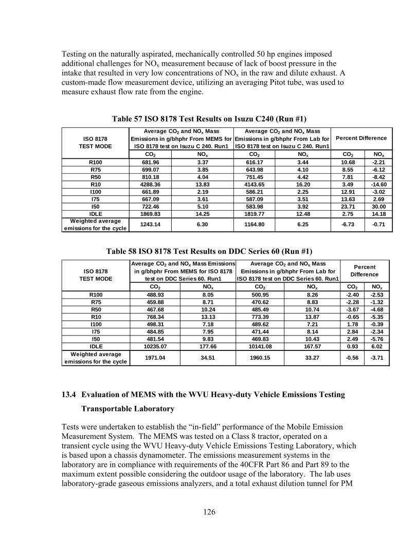
Testing on the naturally aspirated, mechanically controlled 50 hp engines imposed additional challenges for NOx measurement because of lack of boost pressure in the intake that resulted in very low concentrations of NOx in the raw and dilute exhaust. A custom-made flow measurement device, utilizing an averaging Pitot tube, was used to measure exhaust flow rate from the engine.

Table 57 ISO 8178 Test Results on Isuzu C240 (Run #1)

ISO 8178 TEST MODE

Average CO2 and NOx Mass Emissions in g/bhphr From MEMS for

ISO 8178 test on Isuzu C 240. Run1

Average CO2 and NOx Mass Emissions in g/bhphr From Lab for ISO 8178 test on Isuzu C 240. Run1

Percent Difference

CO2 NOx CO2 NOx CO2 NOx

R100 681.96 3.37 616.17 3.44 10.68 -2.21 R75 699.07 3.85 643.98 4.10 8.55 -6.12 R50 810.18 4.04 751.45 4.42 7.81 -8.42 R10 4288.36 13.83 4143.65 16.20 3.49 -14.60 I100 661.89 2.19 586.21 2.25 12.91 -3.02 I75 667.09 3.61 587.09 3.51 13.63 2.69 I50 722.46 5.10 583.98 3.92 23.71 30.00

IDLE 1869.83 14.25 1819.77 12.48 2.75 14.18 Weighted average

emissions for the cycle 1243.14 6.30 1164.80 6.25 -6.73 -0.71

Table 58 ISO 8178 Test Results on DDC Series 60 (Run #1)

ISO 8178 TEST MODE

Average CO2 and NOx Mass Emissions in g/bhphr From MEMS for ISO 8178

test on DDC Series 60. Run1

Average CO2 and NOx Mass Emissions in g/bhphr From Lab for

ISO 8178 test on DDC Series 60. Run1

Percent Difference


R100 488.93 8.05 500.95 8.26 -2.40 -2.53 R75 459.88 8.71 470.62 8.83 -2.28 -1.32 R50 467.68 10.24 485.49 10.74 -3.67 -4.68 R10 768.34 13.13 773.39 13.87 -0.65 -5.35 I100 498.31 7.18 489.62 7.21 1.78 -0.39 I75 484.85 7.95 471.44 8.14 2.84 -2.34 I50 481.54 9.83 469.83 10.43 2.49 -5.76



13.4 Evaluation of MEMS with the WVU Heavy-duty Vehicle Emissions Testing

Transportable Laboratory

Tests were undertaken to establish the “in-field” performance of the Mobile Emission Measurement System. The MEMS was tested on a Class 8 tractor, operated on a transient cycle using the WVU Heavy-duty Vehicle Emissions Testing Laboratory, which is based upon a chassis dynamometer. The emissions measurement systems in the laboratory are in compliance with requirements of the 40CFR Part 86 and Part 89 to the maximum extent possible considering the outdoor usage of the laboratory. The lab uses laboratory-grade gaseous emissions analyzers, and a total exhaust dilution tunnel for PM

126

measurement. Thus, the MEMS was sampling and analyzing raw exhaust samples, and the data generated by the Transportable Lab emanates from dilute samples that are extracted from the total-exhaust dilution tunnel.

Comparing the data from the MEMS with that obtained from a transportable lab completed a major step in the performance evaluation of the MEMS. These tests are imperative for any portable emission measurement system and assist in documenting the response times of the MEMS for in-use testing, in addition to providing a check on the robustness of the MEMS. Although stationary and portable engines are typically thought to operate according to less transient duty cycles than on-road or off-highway engines, most applications would involve significant transient portions of operations, as governors toggle between no-load and loaded conditions, depending upon vocational demands. Moreover, accepting sub-standard transient response performance under the premise that targeted test engines would not likely encounter highly transient operation would be a significant compromise when the research objectives are to develop test methodology, which is inherently related to, and limited by, emissions measurement system performance.

Figure 36 and Figure 37show the continuous mass emission rates (g/sec) of NOx and CO2 over the entire transient chassis dynamometer cycle. The error in mass emission rates of CO2 and NOx as measured by MEMS were within 1% and 5%, respectively. Additional tests were performed to check the precision of the MEMS. The MEMS data was in very good agreement with the laboratory-grade analyzer based system.

13.5 Summary

The WVU MEMS is a proven tool for conducting in-use emissions measurements. The MEMS has been closely scrutinized and extensively evaluated by the US EPA, S-HDDE, and WVU. The MEMS is in a constant state of modifications and improvements as new technology becomes available.

127

1- I

~ ~ Ill'-!, -l ,, """

"'l- - ' ' I,.. I ... Ir" ~

0

0.05

0.1

0.15

0.2

0.25

0.3

0.35 N

Ox (

g/s)

MEMS NOx

Lab NOx

0 100 200 300 400 500 600 700 800 900 1000

Time (sec)

Figure 36 Comparison of MEMS Vs Lab NOx Mass Emission Rate over a WVU 5 Mile Transient Cycle

60

CO

2 (g

/s)

50

40

30

20

10

0

Lab CO2 MEMS CO2

0 100 200 300 400 500 600 700 800 900 1000

Time (sec)

Figure 37 Comparison of MEMS Vs Lab CO2 Mass Emission Rate over a WVU 5 Mile Transient Cycle

128

13.6 WVU Partial Flow-Dilution Tunnel : Determination of Total Particulate

Matter (TPM)

A Detroit Diesel Corporation Series 60 engine was used for the qualification of the mini-dilution tunnel and for the validation runs. As mentioned earlier in this document, partial flow, mini-dilution, and micro-dilution are all terms associated with similar treatment of exhaust gas PM samples. These technologies mimic the interaction of the exhaust sample and, hence, PM formation that is afforded by a full-flow CVS system, but only a portion of the total exhaust gas enters the tunnel. Some manufacturers refer to smaller versions of this design as a micro-tunnel, with the only distinction being tunnel size. The three terms are often encountered in literature interchangeably. Particulate matter measurements were made using the partial flow dilution tunnel and the full-flow double-dilution tunnel at the West Virginia University Engine and Emissions Research Laboratory (WVU EERL) test facility.

Brake-specific particulate matter (BSPM) emissions measurements were obtained by gravimetric analysis of PM samples collected on filters using the partial flow dilution tunnel, and the full flow double-dilution CVS. Results obtained using the mini-tunnel had a difference of approximately ± 15% with that obtained using the full flow dilution tunnel. This is an acceptable error for alternative PM methods. The measurements were more accurate whenever the dilution ratio for the mini-tunnel remained stable for the entire duration of the tests. The instability of the dilution ratio was largely contributed to less-than-optimal performance of the PID control algorithm employed by the system. An optimized system should, therefore, provide improved repeatability and better correlation with the CVS system. Figure 38 shows the comparison of BSPM data obtained using the mini-tunnel and the CVS, and Figure 39 shows the percentage difference between the two.

The error was very high in cases where the dilution ratio could not be held stable. Results seen in Figure 38 and Figure 39 show that the accuracy of the mini-tunnel is very much dependent on the stability of the dilution ratio.

13.6.1 Summary

It is recommended that a partial flow dilution system be used for filter-based gravimetric analysis of PM emissions. Use of pre-packaged and pre-weighed filter cassettes is recommended for in-field measurements. Results to support the use of pre-packaged filters are discussed in the section that presents Method 5 sampling systems.

129

I I I

I I

I I I

I I .I

I I I

C I

I I I

] I .I

I I I

I I I

I I I

I .I

I I I

~ I I

I I I

I I

• I

I I

I I I

I I I

I I I

I I I

I I

r I I

I I

I .d

I I I

% Difference BSPM, g/bhp-hr

0.06

0.05

0.04

0.03

0.02

0.01 0

Figure 39 Percentage Difference betw

een Laboratory-M

ini-tunnel BSPM

M

easurements

130

040903_r100_1

040903_r100_4

041003_r100_3

041103_r100_2

041103_r100_3

041103_r100_4

041303_r100_1

041303_i50_1

041303_m75_1

041303_r100_2

041303_i50_2

041303_m75_2

151050-5

-10

-15

-20

11.5

-17.9

-1.8

0.6

-13.2

-14.8

4.2

-14.5

-10.4

-9.2

-18.0

-15.3

Figure 38 Com

parison of Laboratory-M

ini-tunnel BSPM

Measurem

ents

Test_1

Test_2

Test_3

Test_4

Test_5

Test_6

Test_7

Test_8

Test_9

Test_10

Test_11

Test_12

0.05

0.04

0.04

0.04

0.04

0.05

0.04

0.03

0.04

0.04

0.03

0.04

0.05

0.03

0.04

0.04

0.04

0.04

0.04

0.03

0.04

0.03

0.03

0.03

Lab

Mini-tunnel

13.7 METHOD 5: Determination of Total Particulate Matter (TPM):

Re-iterating the discussion that was presented in the Experimental Equipment and Procedures chapter, the ARB Method 5 document defines PM as “any material that condenses at or above the filtration temperature, determined gravimetrically after removal of uncombined water”. According to the ARB Method 5, matter that is liquid at standard temperature must be included in the determination of TPM. This matter is assumed to pass as gas through the filter and gets condensed in the impingers. Hence, “impinger catch” and “impinger catch extract” are included in the determination of TPM.

It should be noted that other regulatory bodies, such as, the US EPA, do not consider the back half for determination of TPM. Only the front half, that is, “probe catch” and “filter catch” are required to define TPM.

The Method 5 test results are shown below. As mentioned before, the Method 5 data was collected for only two modes of the ISO 8178 test schedule after discussions with the Program Manager. The choice of the two modes was based on the total mass of PM desired, and the limitations imposed by the range of the pressure transducer in the Method 5 system. Additionally, attempts were also made to operate the engine in a “wet mode” (high soluble organic fraction) and a “dry mode” (PM emissions would be dominated by elemental carbon). The results show good correlation with the laboratory procedure of measuring TPM when the back half extraction (BHE) is excluded from PM determination. It may be possible employ the Method 5 analysis for measuring PM from stationary and portable engines operating in the field, but its use for inspection and maintenance type compliance testing appears to be highly impractical.

The following table gives a comparison of the Method 5 data with the laboratory data with and without the back half extraction for the Isuzu C240 and DDC Series 50 engines. Table 59 and Table 60 show that PM emissions captured with the Method 5 sampling train were in good agreement with the regulatory method utilizing the CVS. PM emissions for the two methods were within 8 percent at the R100 operating condition, without the back-half. The R100 mode is expected to generate relatively smaller amounts of SOF. However, with the back-half included in the Method 5 mass calculations, the differences in the two methods deviate by as much as 73% for R100 condition. Similar results were observed at the I100 condition. Without the back-half the PM emissions measured by the Method 5 sampling train, and the CVS based PM samples differed by less than 10%. The differences exceeded 90%, in one of the replicates, when the back-half was included for the I 100 engine operating condition.

PM results from the DDC Series 60 engine show that with the exception of one of the three runs at I50, the brake-specific PM measured by the two methods differed by less than 5%, provided the back-half was not included. The differences were less than 8% for the I75 mode, as well. Again, inclusion of the back-half resulted in differences in excess of 30% between the brake-specific PM emissions measured by the Method 5 sampling train, and the CVS method for the I 75 operating condition.

Results obtained in this study are in good agreement with those obtained by CE-CERT, University of California, Riverside under a CARB funded program. Recognizing the fact

131

I I I I I I I

I I I I I I I

I I I I I I I I I I I I I I I I I I I I I

I I I I I I I I I I I I I I I I I I I I I

that all diesel engines are certified for PM emissions using a diluted exhaust, the following is being suggested for in-field PM emissions measurement:

A diluted exhaust sample may be used to collect samples on a filter for gravimetric analysis. A partial flow dilution tunnel may be used for the purpose.

The Method 5 may be used, if necessary, but only the front half needs to be included to satisfy “equivalency” with the CVS based certification data.

Based upon the results obtained above, the investigators conducted the following tests:

Replaced the gooseneck probe with a multi-hole probe that spanned the diameter of the exhaust stack.

Reduced the probe temperature from 250F to ambient conditions

Investigated the effect of pre-conditioning PM filters, weighing the filters, shipping them out for in-field PM sampling, shipping the ‘shot’ filters back to the laboratory, conditioning them again prior to the post-test weighing. This exercise will be referred to as “No Pre-conditioning of Filters” in the remainder of the text.

The “Modified Method 5” and the test results are discussed below.

Table 59 Method 5 Results for two modes of the ISO 8178 tests on Isuzu C 240

METHOD 5 DATA LAB DATA Percent Error Probe

catch (mg) Filter catch

(mg) Impinger

catch (mg) Impinger catch extract (mg)

Raw exhaust f low rate (scfm)

TPM (g/bhp-hr) W/O BHE

TPM (g/bhp-hr) With BHE TPM (g/bhp-hr) W/O BHE With BHE

R 100 Run 1 7.6 17.8 16.1 2.3 102.01 0.119 0.205 0.129 -7.8 58.9 Run 2 7.9 20 17.1 4.6 101 0.13 0.232 0.134 -3.0 73.1 Run 3 7 22.4 18.6 4.2 103.4 0.132 0.225 0.136 -2.9 65.4

I 100Run 1 6.4 25.5 18.1 0.4 82.53 0.149 0.235 0.155 -3.9 51.6 Run 2 8.4 27.3 14.1 1.5 79.32 0.158 0.228 0.151 4.6 51.0 Run 3 8 20.8 17.3 3.9 88.48 0.154 0.268 0.14 10.0 91.4

Table 60 Method 5 Results for two modes of the ISO 8178 tests on DDC Series 60

METHOD 5 DATA LAB DATA Percent Error Probe

catch (mg) Filter catch

(mg) Impinger

catch (mg) Impinger catch

extract (mg) Raw exhaust

flow rate (scfm) TPM (g/bhp-hr) W/O BHE

TPM (g/bhp-hr) With BHE

TPM (g/bhp-hr) W/O BHE With BHE

I 50 Run 1 2.4 9.1 6.1 7.1 325.57 0.040 0.086 0.038 4.4 124.2 Run 2 3.9 7.2 5.1 6.8 335.503 0.040 0.084 0.040 0.1 107.5 Run 3 2.9 5.3 3.4 2.5 320.28 0.029 0.047 0.036 -19.9 31.9

I 75 Run 1 2.4 14.5 3.8 1.9 430.76 0.056 0.075 0.054 3.3 38.2 Run 2 3.1 15 3.1 1.2 431.72 0.058 0.072 0.063 -7.1 15.0 Run 3 2.4 14.7 4.1 1.4 446.4 0.056 0.075 0.062 -8.3 21.3

132

13.7.1 Modified Method 5 Test:

As shown above, the total PM measured with the CVS, in accordance with the requirements of ISO-8178, and 40 CFR, Part 89, was in very good agreement with the front-half of the Method 5 test protocols. WVU’s findings are supported by the study conducted by researchers at CE-CERT, University of California, Riverside. However, application of the Method 5 PM sampling procedure for in-field / in-use emissions testing of stationary sources can still be challenging. Some of the potential issues that will cause problems during in-field testing are the probe traversal, length of the exhaust pipe (since eight diameters are required upstream of the PM sampling probe and the Pitot tube measurement in accordance with Method 1A), elaborate use of glassware (non-robustness) in M5, unavailability of “conditioned” filters, extraction constrains, etc. Hence, WVU attempted to simplify the current Method 5 procedure and make it user-friendly for stationary sources by employing a multi-hole stainless steel sampling nozzle that spanned the entire diameter of the exhaust stack, instead of a gooseneck nozzle. This measure, if proved successful would not necessitate the traverse of the sampling probe. The sampling probe and the filter box were also maintained at ambient temperatures and at the stipulated temperature of 250ºF. Table 16 on page 67 gives the test matrix for this work. Additionally, a few simple additional tests using this “modified” Method 5 sampling system were also performed to investigate the effect of a modified method of pre-conditioning the PM filters. Instead of following the procedures outlined in 40 CFR, part 89 and ISO 8178, the modified method includes conditioning and weighing of filters in a laboratory, shipping them out to a test site, shipping them back to the laboratory after the test followed by re-conditioning and weighing the filters. The following text refers to this method as “no pre-conditioning of filters”.

Figure 40 : A Multi-hole averaging nozzle on the left and a regular quartz “gooseneck” nozzle on the right.

Figure 40 shows the stainless steel multi-hole averaging nozzle and the regular quartz nozzle that were used for the Method 5 tests on the DDC Series 60 engine.

The aim of the first set of experiments (Test#1 and #2 shown in Table 61, and Test#7 and #8 shown in Table 62) was to determine the effect of a multi-hole sampling nozzle on PM mass analysis. Instead of the regular gooseneck type sampling nozzle, a three-hole

133

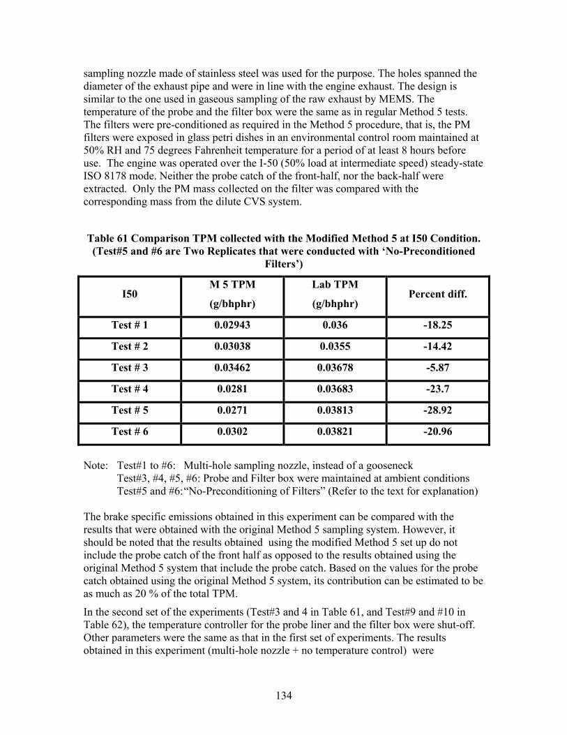
sampling nozzle made of stainless steel was used for the purpose. The holes spanned the diameter of the exhaust pipe and were in line with the engine exhaust. The design is similar to the one used in gaseous sampling of the raw exhaust by MEMS. The temperature of the probe and the filter box were the same as in regular Method 5 tests. The filters were pre-conditioned as required in the Method 5 procedure, that is, the PM filters were exposed in glass petri dishes in an environmental control room maintained at 50% RH and 75 degrees Fahrenheit temperature for a period of at least 8 hours before use. The engine was operated over the I-50 (50% load at intermediate speed) steady-state ISO 8178 mode. Neither the probe catch of the front-half, nor the back-half were extracted. Only the PM mass collected on the filter was compared with the corresponding mass from the dilute CVS system.

Table 61 Comparison TPM collected with the Modified Method 5 at I50 Condition. (Test#5 and #6 are Two Replicates that were conducted with ‘No-Preconditioned

Filters’)

I50 M 5 TPM

(g/bhphr)

Lab TPM

(g/bhphr) Percent diff.

Test # 1 0.02943 0.036 -18.25

Test # 2 0.03038 0.0355 -14.42

Test # 3 0.03462 0.03678 -5.87

Test # 4 0.0281 0.03683 -23.7

Test # 5 0.0271 0.03813 -28.92

Test # 6 0.0302 0.03821 -20.96

Note: Test#1 to #6: Multi-hole sampling nozzle, instead of a gooseneck Test#3, #4, #5, #6: Probe and Filter box were maintained at ambient conditions Test#5 and #6: “No-Preconditioning of Filters” (Refer to the text for explanation)

The brake specific emissions obtained in this experiment can be compared with the results that were obtained with the original Method 5 sampling system. However, it should be noted that the results obtained using the modified Method 5 set up do not include the probe catch of the front half as opposed to the results obtained using the original Method 5 system that include the probe catch. Based on the values for the probe catch obtained using the original Method 5 system, its contribution can be estimated to be as much as 20 % of the total TPM.

In the second set of the experiments (Test#3 and 4 in Table 61, and Test#9 and #10 in Table 62), the temperature controller for the probe liner and the filter box were shut-off. Other parameters were the same as that in the first set of experiments. The results obtained in this experiment (multi-hole nozzle + no temperature control) were

134

comparable with those obtained in the first set where the use of a multi-hole nozzle was the only distinguishing feature.

Tests were performed to investigate the effect of a modified pre-conditioning method for the PM filters. The objective of modifying the filter conditioning procedure was to mimic the time involved in shipping the filters (in filter cassettes or filter holders) when the filters are exposed to ambient temperature and humidity. This exercise could set the pace for shipping out filter cassettes to the in-field site for PM sampling using a mini- or a micro-dilution tunnel, and then shipping the filter cassettes back to a laboratory for gravimetric analysis. To further clarify the “not conditioned” term, all filters actually were conditioned, but not in complete conformance with the requirements of any of the regulatory procedures. The PM filters were first conditioned for 8 hours in an environmental chamber in accordance with requirements of the ISO 8178 and 40 CFR, Part 89, and then weighed. PM filters were placed in filter holders, which were then moved to a location outside the environmental chamber and exposed to ambient temperature and humidity for two days (this would mimic the time required to ship the filters from a laboratory to a test site). Filters were then used in the Method 5 PM sampling routine on the DDC Series 60 engine. After the test, the filters (in the filter holders) were placed outside the environmental chamber for two days again. This would again mimic the time required to ship the filters back to a laboratory. The loaded filters were then conditioned for a standard period of 8 hours, and weighed. Hence, even though the filters were conditioned, authors have adopted the “not conditioned” terminology to distinguish these filters from the others. The data from this set of experiment, test # 5, 6, 11, 12 ( multi hole nozzle + no temperature control over the probe, filter box + “no pre-conditioning) can be compared with test # 3, 4, 9 and 10 ( multi hole nozzle + no temperature control over the probe, filter box ) respectively. Results from the I75 (75 % load at intermediate speed) mode show that the last two replicates, Test#11 and #12, where filters were ‘not conditioned’, the PM results were similar to other tests that used conditioned filters.

In the I75 test series, all tests (#7 through #12) were conducted with the averaging multi-hole sampling nozzle, and Test#9 thru test # 12 were conducted with the probe and filter box at ambient temperature. Conditioned filters were used in Test # 9 and Test # 10 while “No pre-conditioned filters” were used in Test # 11 and Test # 12.The repeatable data from Tests # 9 thru test # 12 suggest that filters may be conditioned and weighed in a lab prior to a test at a remote site; the filters can be packed in filter cassettes that are made of a conducting plastic (or in a regular stainless steel filter holder); shipped out the test site; ‘shot’ in a PM test; shipped back to the chemical laboratory, where the filters are conditioned to the original environmental conditions, and then weighed again.

135

Table 62 Comparison TPM collected with the Modified Method 5 at I75 Condition (Test#11 and #12 are Two Replicates that were conducted with ‘No-Preconditioned

Filters’)

I 75 M5 TPM (g/bhphr) Lab TPM (g/bhphr) Percent diff. Test # 7 0.04285 0.066 -35.07 Test # 8 0.03486 0.066 -47.18 Test # 9 0.04583 0.066 -30.56

Test # 10 0.04535 0.066 -30.23

Test # 11 0.0427 0.066 -33.28

Test # 12 0.04521 0.069 -34.47

Note: Test#7 to #12: Multi-hole sampling nozzle Test#9, #10, #11, #12: Probe and Filter box maintained at ambient conditions Test#11 and #12: “No-Preconditioning of Filters”, plus (Refer to the text for explanation)

13.7.1.1 Summary

All results presented above include brake-specific PM emissions only from the filter catch of the front half. The purpose of modifying the Method 5 was to make the test more ‘user-friendly’ for stationary and portable engines, which may have exhaust stacks as small is 1.5 inches. Extraction of PM from the sampling probe (probe catch) and from the back half were not performed keeping in mind the difficulties associated with such extractions during in-field testing. Results presented in Section 13.7 on Method 5 and CVS-based PM results, highlight the fact the only if the front-half extraction (probe-catch) is included, Method 5 will agree with the CVS-based gravimetric analysis of PM. In addition, results presented in Table 59 and in Table 60, and in Section 13.7 present evidence that any total particulate matter measurement with the Method 5 sampling trains should include the entire front half including the probe catch. Using the information from the regular Method 5 tests, it may be estimated that the front half contribution to TPM is approximately 20%. Hence, it may be concluded that once probe catch were to be included in the analysis, then a multi-hole nozzle along with the probe maintained at ambient temperature could be used for collecting total particulate matter data from stationary and portable engines operating in the field. In fact, if the modified Method 5 results (including the probe catch) are similar to the CVS based and/or mini-tunnel based PM, then the PM measurement may be significantly simplified if a mini-tunnel is used in the field. As mentioned before, the modified Method 5 procedure still requires the use of glass ware, and a delicate, expensive quartz sampling probe. Using such a fragile set up for in-field testing for in-use PM measurements would require very competent handling, since such instruments are prone to breakage. Also, it is likely that many future off-road engines, including the portable & stationary engines, will implement the usage of exhaust after-treatment devices that may significantly change the speciation of PM downstream of the device. The disproportionate amount of soluble organic fraction (SOF) in relation to total particulate matter (on a mass basis) could result in poorer correlation of Method

136

5/Modified Method 5 with CVS dilution tunnel based methods. The use of a mini-dilution tunnel will result in condensation of these hydrocarbons on the filter and would also account for the atmospheric reactions of the particulate matter. This method, since it is mimicking the standard CVS dilution system, could likely provide for better comparison with the standard than the modified Method 5 procedure, which omits the dilution principle.

13.8 AEI Simple Portable On-Vehicle Testing (SPOT) Testing

The exhaust flow rate measurement system of the SPOT is essentially a venturi system. The venturi is inserted in the exhaust exit and secured against the inner wall. Several idle mode tests were performed on a heavy-duty Mack tractor, which was powered by an E7 diesel engine. SPOT’s exhaust flow rate measurement results were compared against MEMS (see Figure 41). The results show that the SPOT unit had clear offset. We believe that this was a software glitch in the system, which can be easily fixed. However, it also highlights that critical importance of implementing a stringent QC/QA protocol for any in-field measurements.

137

I = I

SPOT/MEMS Mass Air Flow Comparison 7/17/03 (MACK) M

ass

Air

Flow

(scf

m)

500.00

450.00

400.00

350.00

300.00

250.00

200.00

150.00

100.00

50.00

0.00 0 0.2 0.4 0.6 0.8 1 1.2

Scaled Time

MEMS SPOT

Figure 41 Comparison of Exhaust Flow Rates Measured by the SPOT and the MEMS on an Idle Test

13.8.1 NOx Emissions

The SPOT uses a Zirconium Oxide (ZrO2) sensor for measurement of NOx emissions. The unit does not include a converter; hence, it measures the entire NO emissions, and upto 83 percent of NO2 emissions [39]. Several on-road tests conducted to evaluate the robustness and accuracy of the SPOT system. These tests produced NOx records, from both MEMS and the SPOT that were in fairly good agreement. A comparison of concentrations is shown Figure 42, Figure 43, and Figure 44. It should be noted that MEMS uses an electrochemical cell for acquiring a redundant QA/QC check for NOx readings. MEMS does include a heated NOx converter immediately downstream of heated filter. Results from the MEMS (using the MEXA 120, and the electrochemical cell), and the SPOT.

MEMS also allows for electrochemical NOx readings. These results are included in Figure 43 and Figure 44.

138

-500

SPOT/MEMS NOx Comparison 7/16/03 (Mack) N

ox (p

pm)

2500

2000

1500

1000

500

0 0 0.1 0.2 0.3 0.4 0.5 0.6 0.7 0.8 0.9 1

Scaled Time

SPOT MEMS

Figure 42 NOx Concentrations Measured by the SPOT and the MEMS During an

On-road NOx Test

SPOT/MEMS NOx Comparison 7/17/03 (MACK)

700.00

NO

x (p

pm)

600.00

500.00

400.00

300.00

200.00

100.00

0.00

MEMS (MEXA)

SPOT

MEMS (Electrochemical)

0 0.1 0.2 0.3 0.4 0.5 0.6 0.7 0.8 0.9 1

Scaled Time

I= I

139

I=

Figure 43 NOx Concentrations Measured by the SPOT and the MEMS (MEXA 120 with a ZrO2 Sensor, and an Electrochemical Cell) During an On-road NOx Test

SPOT/MEMS NOx Comparison (Mack) N

ox (p

pm)

500.00

450.00

400.00

350.00

300.00

250.00

200.00

150.00

100.00

50.00

0.00 0 10 20 30 40 50 60 70 80 90 100

Scaled Time

SPOT NOX MEMS


On-road NOx Test It should be noted that while the MEMS gathers all in-use emissions data at 5 Hz, the SPOT collects data at 1 Hz.

Three, nearly identical, in lab test were preformed on a Mack engine that involved the use of MEMS and SPOT. The results of these three tests can be seen in Figure 45, Figure 46, and Figure 47 below.

13.8.2 Summary

The AEI SPOT system is probably the most portable system that WVU researchers have come across. The system can be attached to the exhaust stack of the engine, and does not require long heated lines, or additional power sources. It should be noted that an ‘end-of-the-stack’ access may not be available, at all, on stationary and portable engines. However, WVU encountered several operational problems with the system, and the calibration files. We understand that AEI is working on a newer design of the SPOT that is more robust, and has significantly expanded capabilities. The newer system, when it is commercially available, should be ideally suited for in-field applications.

140

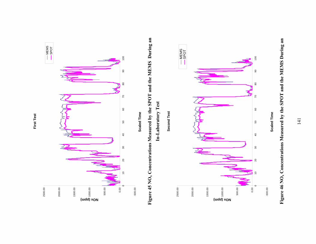
~ ~§ -J

&

~ ~ -J &:

Firs

t Tes

t

-500

.00

0.00

500.

00

1000

.00

1500

.00

2000

.00

2500

.00

0 1

0 20

30 40

50 60

70 80

90 10

0

NOx (ppm) M

EMS

SPO

T

Scal

ed T

ime

Figu

re 4

5 N

Ox C

once

ntra

tions

Mea

sure

d by

the

SPO

T a

nd th

e M

EM

S D

urin

g an

In-L

abor

ator

y T

est

Seco

nd T

est

-500

.00

0.00

500.

00

1000

.00

1500

.00

2000

.00

2500

.00

0 1

0 20

30 40

50 60

70 80

90 10

0

NOx (ppm)

ME

MS

SP

OT

Scal

ed T

ime

Figu

re 4

6 N

Ox C

once

ntra

tions

Mea

sure

d by

the

SPO

T a

nd th

e M

EM

S D

urin

g an

141

I= I

In-Laboratory Test

Third Test

-5.00E+02

0.00E+00

5.00E+02

1.00E+03

1.50E+03

2.00E+03

2.50E+03

0 10 20 30 40 50 60 70 80 90 100

Scaled Time

NO

x (p

pm)

MEMS SPOT


In-Laboratory Test

13.9 Hydrocarbon Analyzer HFID Validation Testing

While diesel engines are known to emit very low levels of hydrocarbons, it is recognized that any regulation requires NOx + HC measurements will require a hydrocarbon analyzer. Only heated flame ionization detectors are considered a valid tool for measuring HC from diesel engines. The Signal Model 3030PM hydrocarbon analyzer was tested at WVU’s Engine and Emissions Research Laboratory (EERL) and the results were compared with a Rosemount Analytical 402 hydrocarbon analyzer, which the EERL is currently using. The Detroit Diesel Corporation Series 60 diesel engine was operated over both the steady state and transient cycles. A 6-mode multipoint steady-state cycle was run for the steady state testing and an USFTP cycle for the transient testing.

Both the Signal and the Rosemount Analytical hydrocarbon analyzers sampled from the same port located in the dilution tunnel. Drawing samples from the same port, allowed for a direct comparison of the analyzers. The Rosemount Analytical 402 analyzer is integrated in the EERL data acquisition system. The system uses a 12 bit analog to digital board to convert the analog signal from the analyzer to a digital output (0 to 2000 ADC code). The analyzers are calibrated with the span value equal to the ADC code of 2000, and the zero value is assigned an ADC code of 0. The EERL assigns channels to each instrument that is used in the Laboratory. The Rosemount Analytical analyzer was

142

-

I --- -- - - ..- - - ,-= -

connected to the permanent hydrocarbon channel in the laboratory, while the Signal was wired into the permanent secondary hydrocarbon channel.

Prior to the test, each analyzer was calibrated. Note that the analyzers display different units of concentration. The Signal analyzer read methane equivalent while the Rosemount Analytical 402 measured percentage of span. Therefore, the Signal read a sample gas of 20 ppm propane as 60 ppm methane equivalent, and the Rosemount Analytical 402 measured the percentage of the span. In the data reduction program, the percent reading of the Rosemount Analytical was converted back to a ppm concentration.

13.9.1 Response Test

A test was run to check the response times for the Rosemount Analytical and Signal hydrocarbon analyzers. A 20 ppm propane span gas was used with helium as the zero air constituent, since helium is hydrocarbon free. A gas divider, Stec, Inc. Model SGD-710C, was used to physically alternate the change in concentration of the sample gas from hydrocarbon free sample to span gas. The sample gas was allowed to stabilize for a minute before the concentration was changed. This step response can be seen in Figure 48 and Figure 49 show a single pulse of the concentration change.

70

65

60

55

50

45

40

ppm35

30

25

20

15

10

5

0

-5 0 200 400 600 800 1000 1200

signal 402 T90 Time

Time (sec)

Figure 48 Response Test using a Span Gas of 20 ppm Propane.

143

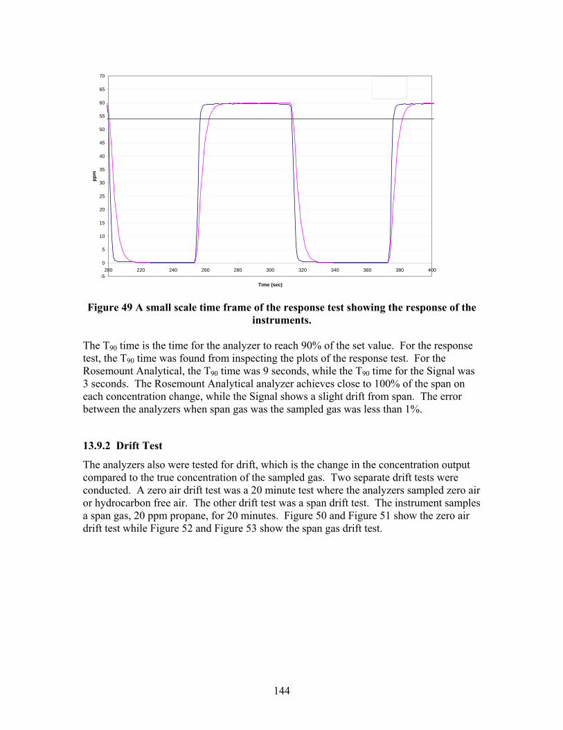
-5

0

5

10

15

20

25

30

35

40

45

50

55

60

65

70

200 220 240 260 280 300 320 340 360 380 400

ppm

signal 402 T90 Time

EJ rr rr I I

\ ,\ Time (sec)

Figure 49 A small scale time frame of the response test showing the response of the instruments.

The T90 time is the time for the analyzer to reach 90% of the set value. For the response test, the T90 time was found from inspecting the plots of the response test. For the Rosemount Analytical, the T90 time was 9 seconds, while the T90 time for the Signal was 3 seconds. The Rosemount Analytical analyzer achieves close to 100% of the span on each concentration change, while the Signal shows a slight drift from span. The error between the analyzers when span gas was the sampled gas was less than 1%.

13.9.2 Drift Test

The analyzers also were tested for drift, which is the change in the concentration output compared to the true concentration of the sampled gas. Two separate drift tests were conducted. A zero air drift test was a 20 minute test where the analyzers sampled zero air or hydrocarbon free air. The other drift test was a span drift test. The instrument samples a span gas, 20 ppm propane, for 20 minutes. Figure 50 and Figure 51 show the zero air drift test while Figure 52 and Figure 53 show the span gas drift test.

144

r r

-2 0 2 4 6 8 10 0 200

400 600

800 1000

1200

ppm

Signal

402 Analyzer

Time (sec)

Figure 50 Hydrocarbon com

parison of the HFID

for a zero air drift test, showing a

scale up to 10 ppm.

-0.12

-0.1

-0.08

-0.06

-0.04

-0.02 0

0.02 0 200

400 600

800 1000

1200

ppm

Signal

402 Analyzer

Time (sec)


parison of the HFID

for a zero air drift test.

145

0 10 20 30 40 50 60

ppm

Signal

402 Analyzer

I

r TT

0 200

400 600

800 1000

1200

Time (sec)


parison of the HFID

for a span drift test.

59.4

59.6

59.8 60

60.2

60.4

60.6

60.8

ppm

Signal

402 Analyzer

0 200

400 600

800 1000

1200

Time (sec)


parison of the HFID

for a span gas drift test, reduced scale.

Figure 50 through Figure 53 show that neither instrum

ent drifts more than 0.6 ppm

. TheSignal M

odel 3030PM analyzer drifts a little m

ore than 0.1ppm during the zero air drift

test and about 0.4ppm for the span gas drift test. The R

osemount A

nalytical 402 analyzer

146

drifts a little more than 0.5ppm for the zero air drift test and a little over 0.4ppm for the span gas drift test. An interesting point is the cyclic drift of the Rosemount Analytical 402 analyzer during the span gas drift test. The Rosemount Analytical has an internal heater that turns on in a cyclic manner to keep the internal oven of the analyzer above the set temperature. This cyclic drift from the Rosemount Analytical 402 is probably a direct result of the cyclic heating of the internal oven.

13.9.3 Transient Tests: USFTP

The USFTP was used to evaluate the Signal Model 3030PM. Several USFTP transient tests were conducted using the Detroit Diesel Corporation Series 60 engine at WVU’s EERL. Hydrocarbon data was collected using both the Rosemount Analytical 402 and Signal Model 3030PM for each test. Figure 54 and Figure 55 show the direct comparison between the Signal and Rosemount Analytical analyzers for two transient tests.

147

ppm

100

90

80

70

60

50

40

30

20

10

0

signal

402

0 200 400 600 800 1000 1200

Time (sec)

Figure 54 Hydrocarbon comparison of the HFID for transient FTP test-1.

0

10

20

30

40

50

60

70

80

90

ppm

signal

402

0 200 400 600 800 1000 1200

Time (sec)

Figure 55 Hydrocarbon comparison of the HFID for transient FTP test-2.

Figure 56 shows a 150 second window of the FTP cycle The Signal Analyzer captured hydrocarbon emissions over most of the transients, where the Rosemount Analytical gave a smoother trace.

148

PPM

0

10

20

30

40

50

60

70

80

90

100 Signal 402

400 420 440 460 480 500 520 540

Time (sec)

I= I

Figure 56 A smaller time scale, an 150 second window, of the Hydrocarbon comparison of the HFID analyzers for transient FTP test-1.

For the transient tests, the R2 values are around 0.70. This value is low when the ideal r-squared value is 1.00. One reason that would account for the low r-squared value is the peak differences between the analyzers. Because of the greater response capabilities of the Signal Analyzer, great differences between the analyzers are found. The peak differences give differences of greater than 100%. If the peak differences are ignored, the mean error between the analyzers would be less than 5%. Therefore, the differences between the Signal and Rosemount Analytical values at peaks and valleys cause data points to be significantly different from the general trend of the data set, thus lowering the r-squared value. The regression analyses, for the two FTP transient tests, are found in Figure 57 and Figure 58.

149

♦

80

R2 = 0.7665 70

Ros

emou

nt A

naly

tical

Mod

el 4

02

60

50

40

30

20

10

0 0 10 20 30 40 50 60 70 80 90 100

Signal Model 3030PM Analyzer

Figure 57 Regression analysis of the HFID analyzers for transient FTP test-1.

70

R2 = 0.7887 60

50

Ros

emou

nt A

naly

tical

Mod

el 4

02

40

30

20

10

0 0 10 20 30 40 50 60 70 80 90

Signal Model 3030PM

Figure 58 Regression analysis of the HFID analyzers for transient FTP test-2.

150

I= I -,.,.. -vv--\rl,J• -~ ..r,....J'

I l

~ _,., . I= I ~ -

- f l

13.9.4 Steady-State Test

Besides FTP transient tests, steady-state test cycles were also run and the hydrocarbon analyzers were compared for these cycles as well. For the steady-state cycles, a DDC Series 60 engine was used, the same engine used for the transient tests. Figure 59 and Figure 60 below show 5 modes in comparison. The 6th mode was idle, and data was not collect over mode-6.

35

30

25

20

15

10

5

0

Signal Model 3030PM Rosemount Analytical Model 402

0 100 200 300 400 500 600 700

time (sec)

ppm

Figure 59 Hydrocarbon comparison of the HFID for steady state 6-mode test-1.

35

30

25

20

15

10

5

0

Signal Model 3030PM Rosemount Analytical Model 402

0 100 200 300 400 500 600

Time (sec)

ppm

Figure 60 Hydrocarbon comparison of the HFID for steady state 6-mode test-2.

From Figure 59 and Figure 60, for a comparison, all the modes matched well except for the second mode, which showed a difference of approximately 6% between the two analyzers. This error is very acceptable.

151

Figure 61 and Figure 62 show that the R-squared value of the regression is above 0.99. The trend line has a slope of around 0.95, which means that that the data from the analyzers do not match exactly, but are close to the same values at each specified time. Note: the trend line is forced through the zero axes, and it is assumed that the trend is a linear trend.

35

R2 = 0.9992 30

25

Ros

emou

nt A

naly

tical

Mod

el 4

02

20

15

10

5

0 0 5 10 15 20 25 30 35

Signal Model 3030PM

Figure 61 Regression analysis of the HFID for steady state 6-mode test-1.

35

R2 = 0.9997 30

25

Ros

emou

nt A

naly

tical

Mod

el 4

02

20

15

10

5

0 0 5 10 15 20 25 30 35

Signal Model 3030PM

Figure 62 Regression analysis of the HFID for steady state 6-mode test-2.

152

13.10 Horiba OBS-1000

Horiba OBS-100 was evaluated using a Mack E7 in an engine test cell. Data was also collected with the WVU MEMS, and laboratory grade analyzers and the CVS in the engine test cell. The engine was operated through the FTP cycle, and over another transient cycle that was developed to faithfully represent on of the on-road routes that were developed for the US EPA and S-HDDE.

Figure 63 through Figure 66 show the continuous NOx and CO2 data as measured with the MEMS, the Horiba OBS 1000 and by the EERL’s laboratory grade equipment. While the MEMS and Horiba OBS1000 measured raw exhaust emissions, the laboratory measured dilute exhaust emissions. While this may introduce some differences in the magnitude of the mass emissions rates due to diffusional and temporal effects associated with the CVS, these differences are not very significant. Also, the Horiba system employed a non-sampling zirconium oxide sensor for NOx measurements. MEMS also uses a zirconium oxide sensor, but the sampled exhaust stream is pre-conditioned through a heated filter and a heated NO2 to NO converter. The WVU system ensures that all of the NOx emissions are measured by the use of the converter, because a zirconium oxide sensor has a 82% response to NO2. Further, WVU measures dry CO2 but report wet reading by using a dry to wet conversion factor. Horiba OBS-100 measures wet CO2 and then corrects for the water using a proprietary wet correction.

Figure 63 and Figure 64 show the continuous (g/s) NOx and CO2, respectively, when the engine was operated over the FTP cycle. Figure 65 and Figure 66 show similar traces for NOx and CO2 when the engine was operated over a cycle that simulated an on-road route. Engine torque and speed were recorded on a continuous basis over an on-road route. This data set was then processed to create an engine dynamometer cycle that was used in this study.

It is evident that the Horiba OBS1000 invariably returned higher mass emission rates than the laboratory or the MEMS. However, the differences are not significant. Table 63 and Table 64 list the mass emission rates (g/s) and brake specific emissions (g/bhp-hr) of NOx and CO2 for the laboratory, MEMS and Horiba OBS1000 when the engine was operated over the FTP and the on-road simulated route. Table 64 highlights a very important aspect of in-use emissions measurements. A comparison of the mass emissions rates shows minimal differences between the laboratory, MEMS and the OBS1000. However, the differences become very significant when the brake specific emissions are reported. The differences arise from the errors in the torque broadcast by the engine ECM. The laboratory torque readings are acquired from a load cell during the cycle operation. However, the torque readings for the portable systems (OBS1000 and MEMS) were acquired from the ECU broadcast, which in itself is a calculated value based upon an estimated fuel consumption. Errors due to inaccurate torque broadcast have been found be significantly greater than those reported in Table 64, particularly for part load engine operating conditions, or over a cycle that does not demand a high average load of the engine.

153

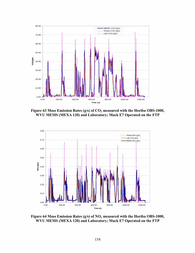
I

'-

I I

..

I , I I

; . ' ) I ' . ' ' ' '

. a•

: . I ' I ' . ~

• •I ' ' ' .,

i ' I I I

ti. & .a...

--- - - .

I -- I

: i ;

,, '

,, ' I

,, ' I ,,

l~ . ,, ,, , ,, • ,, . ,, '

Ji I ' ' ' tel ' '

lffl ' :

; I

;

' ' '

~-I

~ ! L ..at. • I ,.__ - .

80.00 MEMS CO2 (g/s) Horiba CO2 (g/s)

70.00 Lab CO2 (g/s)

60.00

50.00

CO

2 (g

/s)

40.00

30.00

20.00

10.00

0.00 0.00 200.00 400.00 600.00 800.00 1000.00 1200.00

Time (s)

Figure 63 Mass Emission Rates (g/s) of CO2 measured with the Horiba OBS-1000,

WVU MEMS (MEXA 120) and Laboratory; Mack E7 Operated on the FTP

0.80

Horiba NOx (g/s) Lab CO2 (g/s)

0.70 MEMS NOx (g/s)

0.60

0.50

NO

x (g

/s)

0.40

0.30

0.20

0.10

0.00 0.00 200.00 400.00 600.00 800.00 1000.00 1200.00

Time (s )

Figure 64 Mass Emission Rates (g/s) of NOx measured with the Horiba OBS-1000, WVU MEMS (MEXA 120) and Laboratory; Mack E7 Operated on the FTP

154

I

I~ ~~1 l~-t~

'•

,,

I l~

' ~ '• ·• '4

r- I I

h,~ f~

I I

I

Ir :~~ V'i ~-I l-,

0.80

Horiba NOx (g/s)

0.70 Lab CO2 (g/s) MEMS NOx (g/s)

0.60

0.50

NO

x (g

/s)

0.40

0.30

0.20

0.10

0.00 0.00 200.00 400.00 600.00 800.00 1000.00 1200.00

Time (s)

Figure 65 Mass Emission Rates (g/s) of CO2 measured with the Horiba OBS-1000, WVU MEMS (MEXA 120) and Laboratory; Mack E7 Operated on a Simulated On-

road Route

1.20

Horiba NOx (g/s) Lab CO 2 (g/s) Shifted NOx Corr (Mexa) g/s

1.00

0.80

NO

x (g

/s)

0.60

0.40

0.20

0.00 0.00 500.00 1000.00 1500.00 2000.00 2500.00

Time (s)

Figure 66 Mass Emission Rates (g/s) of NOx measured with the Horiba OBS-1000,

WVU MEMS (MEXA 120) and Laboratory; Mack E7 Operated on a Simulated On-road Route

155

Lab MEMS % diff Horiba % diffLab MEMS % diff Horiba % diffLabLab MEMSMEMS % diff% diff HoribaHoriba % diff% diff

Lab MEMS % diff Horiba % diffLab MEMS % diff Horiba % diffLabLab MEMSMEMS % diff% diff HoribaHoriba % diff% diff

IIInnnttteeegggrrraaatttededed W W Wooorkrkrk(((bbbhp-hp-hp-hrhrhr))) 23.823.823.8 232323.1.1.1 3.13.13.1 23.123.123.1 3.13.13.1

AvAvAveeerrraaagggeee CO CO CO222 (g/(g/(g/sss))) 11.311.311.3 101010.4.4.4 7.87.87.8 10.710.710.7 5.35.35.3

AvAvAveeerrraaagggeee NO NO NOxxx ( ( (ggg///sss))) 0.10.10.1 0.10.10.1 -1.9-1.9-1.9 0.120.120.12 -9.1-9.1-9.1

bsCObsCObsCO222 566566566 545454111 4.74.74.7 555555555 2.12.12.1

bsNObsNObsNOxxx 5.55.55.5 5.85.85.8 -5.0-5.0-5.0 6.26.26.2 -12.3-12.3-12.3

InInInttteeegggrrraaattteeeddd W W Wooorrrkkk(((bhpbhpbhp---hhhrrr))) 727272...444 79.79.79.999 9.9.9.888 797979...999 9.9.9.888

AAAvvverereraaaggge Ce Ce COOO222 (g(g(g///sss))) 171717...888 16.16.16.999 -5-5-5...111 16.16.16.989898 4.4.4.999

AAAvvveeerrrageageage N N NOOOxxx ( ( (ggg///sss))) 0.0.0.222 0.0.0.222 1.1.1.888 0.0.0.232323 -1-1-1444...222

bsbsbsCCCOOO222 555555111 474747444 -1-1-1444...999 476476476 141414...666

bsbsbsNNNOOOxxx 6.6.6.222 5.5.5.777 -8-8-8...111 6.6.6.444 -4-4-4...444

Table 63 Comparison of Brake-specific Emissions Measured with the Horiba OBS-1000, WVU MEMS, and Engine Laboratory Over the FTP

Lab MEMS % diff Horiba % diff

Integrated Work (bhp-hr) 23.8 23.1 3.1 23.1 3.1

Average CO2 (g/s) 11.3 10.4 7.8 10.7 5.3

Average NOx (g/s) 0.1 0.1 -1.9 0.12 -9.1

bsCO2 566 541 4.7 555 2.1

bsNOx 5.5 5.8 -5.0 6.2 -12.3

Table 64 Comparison of Brake-specific Emissions Measured with the Horiba OBS-1000, WVU MEMS, and Engine Laboratory over the Bruceton Mills Route

Simulated on an Engine Dynamometer

Lab MEMS % diff Horiba % diff

Integrated Work (bhp-hr) 72.4 79.9 9.8 79.9 9.8

Average CO2 (g/s) 17.8 16.9 -5.1 16.98 4.9

Average NOx (g/s) 0.2 0.2 1.8 0.23 -14.2

bsCO2 551 474 -14.9 476 14.6

bsNOx 6.2 5.7 -8.1 6.4 -4.4

156

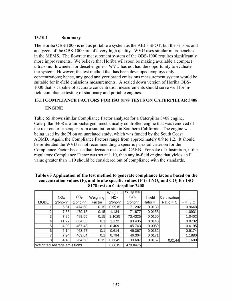
13.10.1 Summary

The Horiba OBS-1000 is not as portable a system as the AEI’s SPOT, but the sensors and analyzers of the OBS-1000 are of a very high quality. WVU uses similar microbenches in the MEMS. The flowrate measurement system of the OBS-1000 requires significantly more improvements. We believe that Horiba will soon be making available a compact ultrasonic flowmeter for diesel engines. WVU has not had the opportunity to evaluate the system. However, the test method that has been developed employs only concentrations; hence, any good analyzer based emissions measurement system would be suitable for in-field emissions measurements. A scaled down version of Horiba OBS-1000 that is capable of accurate concentration measurements should serve well for in-field compliance testing of stationary and portable engines.

13.11 COMPLIANCE FACTORS FOR ISO 8178 TESTS ON CATERPILLAR 3408

ENGINE

Table 65 shows similar Compliance Factor analyses for a Caterpillar 3408 engine. Caterpillar 3408 is a turbocharged, mechanically controlled engine that was removed of the rear end of a scraper from a sanitation site in Southern California. The engine was being used by the PI on an unrelated study, which was funded by the South Coast AQMD. Again, the Compliance Factors range from approximately 0.9 to 1.2. It should be re-iterated the WVU is not recommending a specific pass/fail criterion for the Compliance Factor because that decision rests with CARB. For sake of illustration, if the regulatory Compliance Factor was set at 1.10, then any in-field engine that yields an F value greater than 1.10 should be considered out of compliance with the standards.

Table 65 Application of the test method to generate compliance factors based on the concentration values (F), and brake specific values (F’) of NOx and CO2 for ISO

8178 test on Caterpillar 3408

MODE NOx

g/bhp-hr CO2

g/bhp-hr Weighing

Factor

Weighted NOx

g/bhphr

Weighted CO2

g/bhphr Infield

Ratio = I Certification Ratio = C F = I / C

1 6.61 474.68 0.15 0.9915 71.202 0.0139

0.0144

0.9648 2 7.56 479.18 0.15 1.134 71.877 0.0158 1.0931 3 7.35 489.55 0.15 1.1025 73.4325 0.0150 1.0402 4 11.72 834.35 0.1 1.172 83.435 0.0140 0.9732 5 4.09 457.43 0.1 0.409 45.743 0.0089 0.6195 6 6.14 463.67 0.1 0.614 46.367 0.0132 0.9174 7 7.94 463.04 0.1 0.794 46.304 0.0171 1.1880 8 4.43 264.58 0.15 0.6645 39.687 0.0167 1.1600

Weighted Average emissions 6.8815 478.0475

157

13.12 COMPLIANCE FACTORS FOR A MY1997 HEAVY-DUTY DIESEL

ENGINE FROM A CLASS 8 TRACTOR: FTP AND SIMULATED ON-

ROAD CYCLE TESTED ON AN ENGINE DYNAMOMETER

13.12.1 Quantification of NTE Emissions based on NOx/CO2 Ratios

The uncertainty analysis (described in Chapter 12 ) performed on the MEMS system clearly indicated that the major factor contributing to the total uncertainty is the uncertainty in the flow measurement. With WVU’s experience in on-board, in-use emissions quantification form on-highway vehicles, this team of researchers conducted tests on a MY1997 engine from a Class 8 tractor. The engine was operated on a total of 14 routes, and in-use emissions data were collected with the MEMS to qualify the proposed Compliance Factor method. Both, brake-specific emissions and concentration data were collected. Certification ratio was calculated using the NOx standards for the MY 1997 engine, and the CO2 values were obtained by running the engine on a FTP cycle in the WVU EERL engine laboratory. Analysis was done to calculate the ratio of NOx and CO2 and create a baseline to quantify the NTE emissions based on the ratios. It had been found that the uncertainty in emissions decreases significantly when emissions are expressed as a ratio of NOx and CO2.

The objective of this set of analysis was to establish a factor based upon fuel-specific emissions (for example, NOx/CO2 ratio) that could be used to quantify the not-to-exceed (NTE) emissions. In fact, this on-road investigation was the first in the series of tests and analyses that have been presented in this report. If fuel-specific and brake-specific emissions correlated well, then the approach would be used in this study for the stationary and portable engines. The assumptions and approximations that were adopted in the process are discussed below.

The first step in this analysis was to approximate the certification (heavy-duty FTP cycle) values of CO2. The average value of brake-specific CO2 obtained from the laboratory testing (values published by the manufacturer could be used) was used in calculations. Also, the brake-specific NOx emissions standard corresponding to the engine model year (MY1997) was used. For example, for a MY 1998 engine, a brake-specific NOx value of 4.0 g/bhp-hr would be used whereas for a 1996 engine 5.0 g/bhp-hr should be used. The brake-specific CO2 values used were obtained from the emissions results of FTP cycles when the engine was exercised on the engine dynamometer. The ratio of these two values is the Certification (FTP) NOx/CO2 ratio.

The fuel-specific NOx was calculated as a ratio NOx and CO2 values obtained from the on-road tests for the NTE zone. This ratio was then expressed as a function of the FTP fuel- specific NOx.

To illustrate the determination of the ratio of on-road fuel specific NOx and FTP fuel specific NOx, a MY 1997 engine was considered. The allowable brake-specific NOx value for an FTP test is 5.0 g/bhp-hr. From laboratory testing the average value of brake-specific CO2 obtained for an FTP test was 525 g/bhp-hr. Thus, the FTP fuel-specific NOx (Certification Ratios) was calculated to be 0.0095.

158

As a next step the average value of the fuel-specific NOx (In-field Ratio) was calculated for one of the routes on which the vehicle was tested, and it was found to be 0.0139. The In-field Ratio was then expressed as a function of the Certification Ratio by dividing the In-field Ratio with the Certification Ratio.

On-road (In-field) bsNOx value = 5.85 g/bhp-hr On-road (In-field) bsCO2 value = 487.5 g/bhp-hr In-field Ratio/Certification ratio = 1.26 NTE allowed (per Consent Decrees) limit for bsNOx = 6.25 g/bhp-hr

The calculation of the ratio factor for this MY 1997 engine on different routes is shown in Table 66. Considering the Compliance Factor values (On-road Ratio/FTP Ratio) for the different routes, a pass/fail criterion may be established by a regulatory agency. The value of the Compliance Factor may lie within the range of values calculated from vehicle operation over different routes. In fact, similar tests should be run on a range of engine types, model numbers, model years, and technologies over a wide variety of driving routes, and a database of Compliance Factors should be calculated. The final regulatory pass/fail criterion should be derived from this database.

Table 66 Baseline NOx/CO2 calculations for a MY 1997 engine

Engine Model Year 1997 Allowed FTP bsNOx 5.0000 Allowed FTP bsCO2 525.00

FTP Ratio 0.00950 Allowed NTE bsNOx 6.2500

Route/Leg Maximum On-road ratio/FTP ratio Average On-road ratio/FTP ratioRatio bsNOx Ratio bsNOx

SAB2BM 0.0187 12.73 1.96 0.0139 7.334 1.46 BM2SAB 0.0141 7.241 1.48 0.0141 6.527 1.48 SAB2BM 0.0192 13.52 2.02 0.0144 7.64 1.52 BM2SAB 0.0178 12.10 1.87 0.0149 7.392 1.56 PA1 0.0141 8.722 1.48 0.012 5.851 1.26 PA2 0.0201 10.48 2.11 0.0147 6.808 1.54 PA3 0.0188 9.877 1.97 0.0142 6.844 1.49 PA1 0.0141 7.983 1.46 0.0125 6.110 1.31 PA2 0.0193 13.10 2.02 0.014 7.076 1.47 PA3 0.0189 9.610 1.98 0.0142 6.599 1.49 SAB2SW 0.0139 7.381 1.46 0.0131 6.444 1.38 SW2SAB 0.0149 7.865 1.57 0.0128 6.370 1.34 SAB2SW 0.0152 8.073 1.59 0.0136 6.466 1.43 SW2SAB 0.0167 9.017 1.75 0.0132 6.319 1.39

159

The in-laboratory tests on DDC Series 60 and Isuzu C 240 engines as well as the field tests on a Class 8 Tractor engine have led to the development of a set of Compliance Factors that give a better picture of conformance to emission standards during in use operation. CARB could possibly use the data generated in this report as a basis for, (i) conducting additional tests on a larger population of engines and (ii) develop a pass/fail criterion for in-use compliance of stationary and portable engines.

13.13 In-field Testing

In-use emissions testing were performed to validate the proposed test method. Two engines that fall under the “Portable & Stationary Engines” category were selected. A Multiquip-Whisperwatt diesel powered AC generator and a SullAir 185 diesel powered air compressor were rented for the study. The generator was loaded using a thermostatically controlled room heater while a jack hammer was used to load the air compressor. Thus, both the engines were tested during their “in-use” duty cycle. Emissions data was collected using laboratory grade analyzers mounted on a transportable lab and the MEMS-the portable emission measurement system built by WVU. Both gaseous and particulate matter during “In-use” operation was collected. Two runs were performed for each test engine.

The following tables give the specifications of the test engines.

Table 67 Specification of the Multiquip-Whisperwatt Generator

Multiquip-Whisperwatt Diesel Powered AC Generator

Model DCA-44SPXI

Generator Model DB-0667I

Phase Single

Frequency 60 Hz

Rated output 35 kW

Rated voltage 120 V 240 V

Rated current 182 A 182 A

Power factor 0.8

Engine Model 1990 Isuzu QD-100 (4BD1)

Type 4 cylinders, 4 stroke

Rated Output 56 hp @ 1800 rpm

Displacement 3853 cc

Fuel tank capacity 23.8 gallons

160

Table 68 Specification of the SullAir 185 Air Compressor

SullAir 185 Diesel Powered Air Compressor

Model 2002 SullAir 185

Rated capacity and Pressure

185 CFM @ 100 PSIG (87L/s @ 7 Bar)

Maximum Pressure 125 PSIG @8.5 Bar

Rated Output 51.9 kW @ 2200 rpm

Engine Model 2001 Perkins

Type 4 Stroke 4 cylinders

Rated Output 51.9 @ 2200 rpm

Displacement 3.9L

Idle 800 RPM

Minimum Idle 1700 RPM

Figure 67 Multiquip-Whisperwatt Diesel Powered AC Generator being tested for In-Use Emissions

161

Figure 68 Front view of the Generator. At the background is the transportable lab used for emissions measurement.

The emissions from the two engines have been expressed as grams per unit of time. As mentioned before, measurement of work output from such mechanically controlled engines is fraught with errors and any exercise to quantify these emissions in brake specific terms will result in inaccurate measurements. Hence, emissions have expressed in mass emission rate units. Table 49 and Table 50 give the average emissions recorded for each cycle while Figure 69 through Figure 78 provide a continuous comparison of mass emission rates measured by MEMS versus the Lab. While CO2 was measured within 5 % for all the runs, NOx was measured within 8% of the lab for most of the tests.

Figure 77 and Figure 78 provide an expanded view of the comparison for a section of the test cycle.

Table 51 through Table 54 show the application of the Compliance Factor concept on the two in-field test engines. The Isuzu QD 100 - built in 1990, was not designed to conform to any emissions standards for Off-road engines while the Perkins - built post emissions standards promulgation, was expected to comply with pertinent emissions regulations. However, “In-use” operation can be markedly different from certification cycles and engines certified on certification cycle can emit 2-3 times more during “In-use” condition.

162

I? ';

ll

[ i\

CO2 (g/s)

7654

ME

MS

CO

2 3

Lab CO

2 210 0

200 400

600 800

1000 1200

1400 1600

1800

Time (secs)

Figure 69 Com

parison Of C

O2 M

ass Em

ission Rates From

ME

MS &

Lab D

uring

NOx (g/s)

In-Use O

peration Of T

he Generator. R

un 1

0.12

0.1

0.08

0.06

ME

MS

NO

x 0.04

Lab NO

x

0.02 0 0 200

400 600

800 1000

1200 1400

1600 1800

Time (secs)

Figure 70 Com

parison Of N

Ox M

ass Em

ission Rates From

ME

MS &

Lab D

uringIn-U

se Operation O

f The G

enerator. Run 1

163

I ! I !

0123456

CO2 (g /s )

ME

MS

CO

2La

b C

O2

0 20

0 40

0 60

0 80

0 10

00

1200

14

00

1600

18

00

Tim

e (s

ecs)

Figu

re 7

1 C

ompa

riso

n O

f CO

2 Mas

s Em

issi

on R

ates

Fro

m M

EM

S &

Lab

Dur

ing

In-U

se O

pera

tion

Of

The

Gen

erat

or. R

un 2

0.00

0.02

0.04

0.06

0.08

0.10

0.12

NOx (g /s )

ME

MS

NO

xLa

b N

Ox

0 20

0 40

0 60

0 80

0 10

00

1200

14

00

1600

18

00

Tim

e (s

ecs)

Figu

re 7

2 C

ompa

riso

n O

f N

Ox M

ass E

mis

sion

Rat

es F

rom

ME

MS

& L

ab D

urin

gIn

-Use

Ope

ratio

n O

f T

he G

ener

ator

. Run

2

164

7.0

6.0

CO

2 (g/

s) 5.0

4.0

3.0

MEMS CO2 Lab CO2

2.0

1.0 0 200 400 600 800 1000

Time (secs)

1200 1400 1600 1800

Figure 73 Comparison Of CO2 Mass Emission Rates From MEMS & Lab During

In-Use Operation Of The Air Compressor. Run 1

0.09

0.08

0.07

0.06

NO

x (g/

s)

0.05

0.04

0.03

MEMS NOx Lab NOx

0.02

0.01

0.00 0 200 400 600 800 1000 1200 1400 1600 1800

Time (secs)

Figure 74 Comparison Of NOx Mass Emission Rates From MEMS & Lab During In-Use Operation Of The Air Compressor. Run 1

165

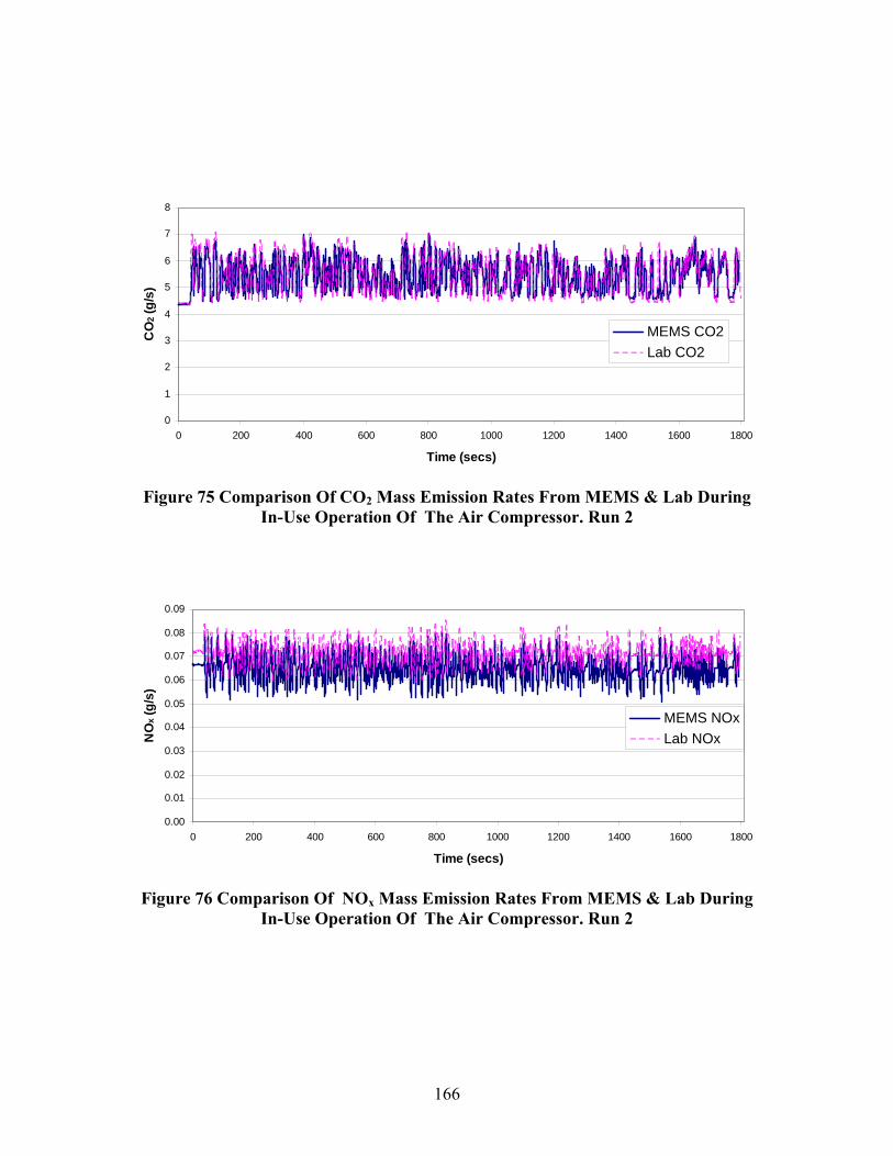
0

1

2

3

4

5

6

7

8

0 200 400 600 800 1000 1200 1400 1600 1800

Time (secs)

CO

2 (g/

s)

MEMS CO2 Lab CO2

Figure 75 Comparison Of CO2 Mass Emission Rates From MEMS & Lab During In-Use Operation Of The Air Compressor. Run 2

0.09

0.08

0.07

0.06

NO

x (g/

s)

0.05

0.04

0.03

0.02

0.01

0.00

MEMS NOx Lab NOx

0 200 400 600 800 1000 1200 1400 1600 1800

Time (secs)

Figure 76 Comparison Of NOx Mass Emission Rates From MEMS & Lab During In-Use Operation Of The Air Compressor. Run 2

166

0

1

2

3

4

5

6

7

8

CO

2 (g

/s)

Lab CO2 MEMS CO2

0 50 100 150 200 250 300 350 400 450 500

Time (secs)

Figure 77 Comparison Of CO2 Mass Emission Rates From MEMS & Lab For a Section Of The In-Use Test On The Air Compressor. Run 2

0.09

0.08

0.07

0.06

NO

x (g

/s)

0.05

0.04

0.03

0.02

0.01

0

Lab NOx MEMS NOx

0 50 100 150 200 250 300 350 400 450

Time (secs)

Figure 78 Comparison Of NOx Mass Emission Rates From MEMS & Lab For a Section Of The In-Use Test On The Air Compressor. Run 2

167

500

The certification ratio (brake-specific) for these two engines is obtained from the brake specific NOx and CO2 emissions observed during laboratory evaluation of the Isuzu C 240 engine on an ISO 8178 test cycle. Since the Isuzu C 240 was of similar size and type as the Isuzu QD 100 and the Perkins engine, the certification ratios for these two engines were chosen to be identical to that of the Isuzu C 240. The certification ratio values were chosen only to illustrate the application of the compliance factor concept. Actual in-use emissions test would require the manufacturer to report the brake specific emissions values for NOx and CO2.

Figure 79 SullAir 185 Diesel powered Air Compressor Being Tested For In-use Emissions

14 Conclusions and Recommendations

Conclusions of this study may presented in the form of recommendations regarding the test method, developed in this study, which CARB could use for determining in-use compliance of stationary and portable engines. These recommendations are listed below:

• In-use Emissions Compliance

• In-use Emissions Measurement Tools (Portable and Stationary Engines)

• In-field Emissions Measurement Standard Operating Procedure

168

14.1 In-use Emissions Compliance Recommendations

Based upon the research conducted on the CARB Stationary and Portable Engine Study and the ‘state-of-the-art’, WVU makes the following recommendations:

The Compliance Factor concept should be employed to determine compliance of stationary and portable engines. This method uses the In-field Ratio of NOx and CO2 concentrations (to obtain mass emissions of NOx and CO2 ) as measured from engines operating in the field, and the Certification Ratio of NOx and CO2 (brake-specific emissions) values from engine certification tests. A ratio of the In-field Ratio and the Certification Ratio gives the Compliance Factor.

In summary,

• If BSFC data for an engine were to be available (it is likely, that it will not be), its validity may be in question because of engine deterioration. Hence, brake-specific emissions data will be un-reliable.

• Therefore, fuel-specific/CO2-specific measurements should be used as a compliance tool. This will require only concentration measurements. Uncertainties due to flow rate measurement and torque/percent load will be avoided. In-field fuel-specific measurements (NOx/CO2) should be compared with the laboratory-generated 8-mode cycle fuel-specific emissions data. Again, in-field fuel-specific emissions should not exceed the Compliance Factor (F) pass/fail criterion determined by CARB. That is the in-field emissions limits should not exceed the product of F and the weighted limits for the ISO 8178 certification test data based fuel-specific emissions.

• For electronic control unit equipped engines, in-use brake-specific emissions should not exceed the product of F and the weighted limits for the ISO 8178 test applicable to the engine being tested.

14.2 In-use Emissions Measurement Tools (Portable and Stationary Engines)

The recommended Compliance Factor method would require measurement of only concentrations for the gaseous pollutant, total particulate matter. Hence, an accurate, reliable and a portable gas concentration measurement analyzer would serve well. A filter-based gravimetric method using pre-conditioned and pre-weighed filter cassettes, and a micro-dilution tunnel is recommended for PM measurements. A modified Method 5 (with the front-half extraction) sampling train could be used, but the tediousness of the process could be avoided by using a micro-dilution tunnel because both procedures yield similar results

Equipment recommendations to conduct the proposed in-field test are as follows:

• PM Measurement

• Filter-based gravimetric PM measurement (using a portable mini-dilution tunnel, or a micro-dilution tunnel)

169




• (NOx – Microflow NDIR soon to be available from Horiba; Non-dispersive ultra-violet analyzer from ABB)




• Short heated sample line(s), heated head pump maintained at temperatures required by CFR 40, Part 89, if non-sampling type sensors are not used.

• Power Supply

• Portable batter packs



Authors believe that measurement of mass emissions is not necessary for determining compliance with the emissions standards. However, if mass emissions measurements are essential and desired, the following recommendations are being made:

• Exhaust Flowrate Measurements


• (Portable ultra-sonic flow meter expected from Horiba)

• PM Measurement

170

• Filter-based gravimetric PM measurement (using a portable mini-dilution tunnel, such as the University of Darmstadt system)




• (NOx – Microflow NDIR soon to be available from Horiba)




• Heated sample line(s), heated head pump maintained at temperatures required by CFR 40, Part 89, if non-sampling type sensors are not used.

Torque Measurement

• Inference from ECU data if available

• From BSFC data, if available, for the engine. But, this data is always suspect because of engine and fueling system wear and tear, mal-maintenance, and possible engine re-builds since the original engine certification.

Electrical Power Supply


Data Acquisition


171

14.3 In-field Emissions Measurement Standard Operating Procedure

A Standard Operating Procedure (SOP) for a complete mass emissions measurement procedure is presented below. If the recommendations made in this report were to be followed, then flowrate measurement, the engine load and speed data are not required:

• Identify the test engine, and collect engine description (make, model, serial number, etc.) prior to site visit to “check-out” the engine.

• Ensure that the engine is in good working condition. This includes inspection of the engine air filter and exhaust system.

• A partially blocked air filter will have an adverse affect on the performance and emissions of an engine. The engine response must be a compromise between de-rating power, or reducing the air/fuel ratio, leading to elevated CO and PM emissions. If there is reason to suspect a problem, the default protocol is to install a new air filter prior to an emissions test.

• Leaking exhaust systems will result in erroneously low reported mass emissions data.

• Collect engine certification and performance data from the manufacturer.

• Transport portable gaseous and PM emissions measurement equipment, sample handling and conditioning systems, data acquisition, data archival and data analysis systems to the field

• (Exhaust flow rate measurement systems also need to be transported, if mass emission rates are to be measured).

• Prepare the engine for testing. That is, get access to the exhaust stack. Implement personnel safety protocols around the engine.

• (Install flow meter on the engine exhaust stack)

Note: Engine exhaust flow rate measurement could be accomplished by approximately two different differential pressure measurement ranges. The compromise in resolution is likely worth the effort afforded to continuously change and recalibrate different sensors (factoring in leakage, calibration errors, etc.)

• Install sampling probes and connect to the sample conditioning system/analyzers using heated lines.

• Connect data acquisition and control system (DAC) to the measurement systems.

• Power-up, warm-up and stabilize the concentration measurement analyzers, PM mass measurement systems, heated lines, DAC, etc.

172

• Leak-check the systems.

• Zero and span the analyzers

• Calibrate the analyzers.

• Warm-up the engine as follows:

• Idle (10 minutes, at least)

• Increase load in two increments and maintain the engine operating condition at each load for a period of 10 minutes, or until oil and coolant temperatures stabilize. It should be noted that some engines may not have temperature gages.

• It should be noted that given the engine application, it might not be possible to increase the load on the engine. In such instances, the engine should be allowed to operate at high idle for 20 minutes.

• Operate the engine over steady-state and transient modes of operation and collect emissions data (gaseous concentration, PM data, flow rates, engine speed, etc.). The actual engine operation will be dependent upon its intended application. The engine application may impose limitations upon how the engine may be operated for emissions testing purposes.

• Emissions data, especially PM, should be collected for at least 20 minutes.

• Multiple tests should be staged such that similar engine pre-test conditioning is afforded.

• Stationary and portable engines in the future will most likely be equipped with exhaust after-treatment devices such as catalytic converters or particulate traps. It should be noted that the effect of previous operating conditions (prior to the beginning of the compliance test) may be observed during an emissions test. For example, a long period of idling the engine prior to a test may result in increase emissions during the test.

• Collect a fuel sample (2 quarts) for standard fuel analysis

• The properties and composition of the fuel can greatly influence emissions levels. WVU performed tests in early 2003 using different commercially available on-road diesel #2 from local fueling stations. NOx emissions varied up to 10% from fuel to fuel over the same test performed in an engine test cell. Fuel analysis should be performed on each new batch of fuel.

173

• Similarly, engine oil properties can influence emissions. In order to assure that in-field emissions tests are comparable and repeatable, it will be necessary to account for or control the influence of varying engine oil properties.

Note: Local fuel quality can be very problematic. WVU has shown that there is a 10% variation in the NOx from one pump to the next. However, fuel analysis will show the reason(s) (aromatics) for this.

• Archive the data for off-site analysis.

• Dissemble emissions measurement equipment.

• Conduct final engine/equipment inspection to ensure that the engine is returned to pre-test condition.

14.4 Recommendation of Future Research Activities

In order to further develop test methods for stationary and portable engine emissions, WVU believes that future research efforts should focus on specific objectives. These objectives have been identified as a result of the research findings reported under the present study.

A larger data base needs to be established in order to validate the proposed compliance factor methodology. Not only does such additional testing and analysis verify the methodology, but this too would assist in identifying a critical value for the compliance factor that could ultimately be used to establish non-compliant in-use engines. More specifically, the compliance factor, as presented herein, merely involves a ratio of the in-field NOx/CO2 concentrations to values of NOx/CO2 concentrations that are averaged over the ISO certification test cycle. This value must then be compared to some established compliance value, that would account for various stochastic tolerances of all components involved. For instance, certification data variability exists, and this could be caused by engine-to-engine emissions production variability as well as laboratory-to-laboratory emission measurement variability. An increased number of tests, as well as analysis of currently available emissions data, could serve to identify the level of accuracy and precision for emissions certification data as well as actual engine emissions production variability. Similarly, the accuracy and precision of the compliance methodology and hardware proposed by this study should also be identified. Only after a thorough investigation of total compliance variability could a value be established to which the compliance factor could be compared with to identify non-compliant performance of an in-use engine.

Specifically, WVU suggests that an inter-laboratory comparison, involving agencies such as MTA/CARB, SWRI, WVU, and Environment Canada be performed in order to quantify the accuracy and precision of current “certification quality” emissions measurement facilities. Such “round-robin” testing would be critical to establishing a compliant standard. In addition, analysis of available manufacturer’s data on new production engines could assist in quantifying variability of new engine emissions data. A proposed survey of emissions from a number of current in-use engines (using the in-

174

field emissions testing methodology prescribed by this study) of various sizes and from a variety of manufacturers could help to establish the variability of in-use engine emissions, owing to various components – wear, maintenance, etc. Finally, a rigorous test of compliance level emissions measurement devices (such as the system used for this project as well as other currently available, comparable systems) must be performed to identify variability of the in-field test equipment. Only after such thorough investigation and integration of the quantitative results, could a value be established with which the compliance factor, prescribed herein, be compared to ultimately identify non-compliant engines in a pass/fail manner.

Extension of the test methodology reported herein to included PM measurements would also need further investigation. WVU would propose a PM methodology based upon a mini-dilution technique. This dilution system would provide for gravimetric-based PM concentrations that could be integrated with engine exhaust flow rate to arrive a PM mass emissions data. The exhaust flowrate could be measured either directly, or by more simply measuring or estimating engine intake air mass flow rates. The methodology would have to be devised with the sampling system as the governing parameter, since in-field compliance tests would inherently necessitate simple and robust measurement systems. With this in mind, the proposed approach would also require an in-depth analysis to identify variability of the methodology before the inevitable development of a compliance criteria could be established. Not only would system limitations need to be identified, but variability associated with limitations of human and equipment performance would need to be quantified.

The WVU investigators have a practical view of the approach for measurement PM, but would propose to take a fundamental approach to describing and understanding the variation in the PM mass measured. PM mass, M, depends on a string of partial derivatives of the relevant variables and on the changes in those variables themselves. For example,

dM = (dM/dP1)dP1 + (dM/dP2)dP2 +……. + (dM/dT1)dT1 + ……(dM/dF1)dF1 +…… + (dM/dx1)dx1 +…

where M is the PM measured mass, where the variables Pi ,Ti and Fi denote pressures, temperatures and flowrates at carefully selected points in the sampling system, and where the xi denote geometric variables. The skill is in selecting reasonable and independent variables. The geometric variables must be chosen carefully to represent all major variations in the size, length and arrangement of the engine exhaust transfer pipe, primary tunnel, secondary tunnel and filter holder. The geometric variables must also be sufficient to identify reasonably the true effects of sampling system geometry, but must be constrained to be easily quantifiable and acceptable in number. Additional variables may be required to describe heat transfer, or perhaps the problem can be treated as two separate cases, such as “uninsulated” and “insulated,” in a section of the sampling system. Other factors also need to be considered as cases, such as the type of filter medium used. Variables such as dilution ratio or face velocity will prove to be dependent on the set of independent temperatures, pressures, flowrates and geometry parameters that are used. Each partial differential in the equation can be determined using dedicated sub-models and careful experimentation, and in this way the variability in mass can be

175

attributed directly to the variabilities in the independent variables. These variabilities may be intentional differences in setpoints and sampling system construction between different laboratories, or they may represent the limits of precision in the control of the variables in a laboratory.

Discernable laboratory-to-laboratory and run-to-run variations in PM mass emissions measurements can be attributed to a number of independent variables. These variables include obvious one-dimensional quantities, such as temperatures, pressures and flowrates at critical points in the sampling system, factors that affect the engine operation, and multi-dimensional quantities that describe geometry and materials. With this in mind, WVU proposes that the major effects that cause variability in PM measurement for any sampling system can be narrowed to three basic components. First, there is deposition of exhaust species on the dilution tunnel walls and throughout the sampling system, coupled with subsequent desorption and shedding of particles from the walls. Second, there are physical, controllable variables such as temperature, humidity, flowrate and pressure that influence particle formation and the filtration process itself. Third, there are unpredictable differences associated both with variability in engine operation and with inaccuracies in the weighing process.

176

15 References

1. Reducing Air Pollution from Nonroad engines-Program update. (EPA 420-F-03-011, April 2003).

2. Code of Federal Regulations, Title 40, Part 89 – Control of Emissions from New and In-Use Nonroad Engines; Gaseous and Particulate Exhaust Test Procedures, 1998.

3. “Control of Air Pollution from New Motor Vehicles: Proposed Heavy-Duty Engine and Vehicle Standards and Highway Diesel Fuel Sulfur Control Requirements,” EPA, 40 CFR parts 69, 80,and 86, June 2, 2000.

4. Diesel Exhaust in the United States. (EPA 420-F-03-022, June 2003). 5. Ozturk, S., McKinnon, D.L., Puliafito, J.L., Irigo, C., and Sans, J., (1994),

"International Experience Using Diesel Catalytic Converters for Urban Buses", SAE 940238.

6. EPA Emission Standards Reference Guide for Heavy-Duty and Nonroad Engines, <http://www.epa.gov/omswww/.

7. Gautam, M., Thompson, G. J., Clark, N. N., Riddle, W. C., Carder, D. K., "Development of a Test Method to Measure Stationary and Portable Engine Emissions,” Task I Report Submitted to California Air Resources Board, Department of Mechanical and Aerospace Engineering, West Virginia University, Morgantown, WV, January 3, 2002.

8. Code of Federal Regulations, Title 40, Part 86, Subpart N – Emission Regulations for New Otto-Cycle and Diesel Heavy-Duty Engines; Gaseous and Particulate Exhaust Test Procedures, 1998.

9. 3030PM Portable Heated VOC Analyser Operating Manual, The Signal Instrument Co, Ltd., First Edition, December 1, 1993, Surrey, England.

10. Czachura,B., (2001), Personal Communications. Analytical Engineering Inc., Columbus, In.

11. Czachura,B., Brandon, L., May, Al., (2001), “ Demonstration of the Simple Portable, On-vehicle Testing (SPOT) system on a class 8 vehicle”, Proceedings of the 11th On-road Vehicle Emissions workshop, San Diego, Ca.

12. "Notice of Filing of Consent Decree Under the Clean Air Act," Federal Register, Vol. 63, No. 212, Office of the Federal Register, National Achieves and Records Administration, Washington DC, November 3, 1998.

13. Riddle, W. C., “Design and Evaluation of the Emissions Measurement Components for a Heavy-Duty Diesel Powered Vehicle Mobile Emissions Measurement System (MEMS),” M.S. Thesis, Department of Mechanical and Aerospace Engineering, West Virginia University, Morgantown, WV, 2001.

14. Mohr, M., and Lehmann, U, (2003), “Comparison Study of Particle Measurement Systems for Future Type Approval Application”, Swiss Contribution to Particle Measurement Programme; GRPE-PMP-CH5.

15. Gautam, M., Clark, N. N., Thompson, G. J., Lyons, D. W., “Assessment of Mobile Monitoring Technologies for Heavy-Duty Vehicle Emissions,” Department of Mechanical and Aerospace Engineering, West Virginia University, Morgantown, WV, 1999.

177

http://www.epa.gov/omswww

16. Branstetter, R., Burrahm, R., and Dietzmann, H., "Relationship of Underground Diesel Engine Maintenance to Emissions," Final Report for 1978 to 1983 to the U.S. Bureau of Mines, Department of the Interior Contract H0292009, 1983.

17. Chan, L., Carlson, D. H., and Johnson, J. H., "Evaluation and Application of a Portable Tailpipe Emissions Measurement Apparatus for Field Use," SAE Technical Paper No. 921647, 1992.

18. Spears, M. W., "An Emissions-Assisted Maintenance Procedure for Diesel-Powered Equipment," University of Minnesota, Center for Diesel Research, Minneapolis, MN, 1997.

19. Englund, M. S., "Field Compatible NOx Emission Measurement Technique," SAE Technical Paper No. 820647, 1982.

20. Human, D.M. and Ullman, T. L., “Development of an I/M Short Emissions Test for Buses,” SAE Technical Paper No. 920727, 1992.

21. Kelly, N. A. and Groblicki, P. J., "Real-world Emissions from a Modern Production Vehicle Driven in Los Angeles," Journal of the Air & Waste Management Association, Vol. 43, No. 10, 1993.

22. Mackay, G. I., Nadler, S. D., Karecki, D. R., Schiff, H. I., Butler, J. W., Gierczak, C. A., and Jesion, G., "Dynamometer Intercomparison of Automobile Exhaust Gas CO/CO2 Ratios and Temperature Between On-Board Measurements and a Remote Sensing Near Infrared Diode Laser System," Phase 1b Report to the Coordinating Research Council and National Renewable Energy Laboratory, 1994.

23. Mackay, G. I., Nadler, S. D., Karecki, D. R., Schiff, H. I., Butler, J. W., Gierczak, C. A., and Jesion, G., "Test Track Intercomparison of Automobile Exhaust Gas CO/CO2 Ratios and Temperature Between On-Board Measurements and a Remote Sensing Near Infrared Diode Laser System," Phase 1c Report to the Coordinating Research Council and National Renewable Energy Laboratory, 1994.

24. Butler, J. W., Gierczak, C. A., Jesion, G., Stedman, D. H., and Lesko, J. M., "On-Road NOx Emissions Intercomparison of On-Board Measurements and Remote Sensing," Final Report, Coordinating Research Council, Inc., Atlanta, GA, CRC Report No. VE-11-6, 1994.

25. Gierczak, C. A., Jesion, G, Piatak, J. W., and Butler, J. W., "On-Board Vehicle Emissions Measurement Program," Final Report, Coordinating Research Council, Inc., Atlanta, GA, CRC Report No. VE-11-1, 1994.

26. Real-Time Emissions Measurement System, AC Propulsion Inc., website, September 22, 2003, <http://www.acpropulsion.com/Products/Emissions_Meas.htm>.

27. Bentz, A. P. and Weaver, E., "Marine Diesel Exhaust Emissions Measured by Portable Instruments," SAE Technical Paper No. 941784, 1994.

28. Bentz, A. P., "Final Summary Report on Project 3310, Marine Diesel Exhaust Emissions (Alternative Fuels)," United States Department of Transportation United States Coast Guard Systems, Report No. CG-D-08-98, 1997.

29. Vojtisek-Lom, M. and Cobb, Jr., J. T., "On-Road Light-Duty Vehicle Mass Emission Measurements Using a Novel Inexpensive On-Board Portable System,"

178

http://www.acpropulsion.com/Products/Emissions_Meas.htm

Proceedings of the Eighth CRC On-Road Vehicle Workshop, San Diego, CA, April 20-22, 1998.

30. Pelkmans, L., De Keukeleere, D., Bruneel, H., and Lenaers, G., “Influence of Vehicle Test Cycle Characteristics on Fuel Consumption and Emissions of City Buses,” SAE Conference Paper No. 01FL-308, 2001.

31. Jimenez, J. L., Mcrae, G. J., Nelson, D. D., Zahniser, M. S., and Kolb, C. E., “ Final Report: Remote Sensing of NO and NO2 Emissions from Heavy-Duty Diesel Trucks Using Tunable Diode Lasers,” National Center for Environmental Research, EPA Grant No. R824794, 1998.

32. "Construction Equipment Retrofit Project," Northeast States for Coordinated Air Use Management, Boston, MA, 1998.

33. Butler, J. W., Kornisk, T. J., Reading, A. R., and Kotenko, T. L., "Generating Dynamometer Quality Data On-board Vehicles for Real-World Emission Measurements," Proceedings of the Ninth CRC On-Road Vehicle Workshop, April 19-21, San Diego, CA, 1999.

34. Gautam, M., Clark, N. N., Thompson, G. J., Carder, D. K., Lyons, D. W., “Evaluation of Mobile Monitoring Technologies for Heavy-Duty Diesel-Powered Vehicle Emissions,” Department of Mechanical and Aerospace Engineering, West Virginia University, Morgantown, WV, 2000.

35. Fulper, C., and Spears, M., “Portable Emission Measurement System (PEMS),” Proceedings of the 11th CRC On-Road Vehicle Emissions Workshop, 2001. NO is measured with a divided detection cell in a dedicated sample tube, using the same principle.

36. Kihara, N., Tsukamoto, T., Mastumoto, K., Ishida, K., Kon, M., and Murase, T., “Real-Time On-Board Measurement of Mass Emission of NOx, Fuel Consumption, Road Load, and Engine Output for Diesel Vehicles,” SAE Technical Paper No. 2000-01-1141, 2000.

37. Jetter, J., Maeshiro, S., Hatcho, S., and Klebba, R., “Development of an On-Board Analyzer for Use on Advanced Low Emission Vehicles,” SAE Technical Paper No. 2000-01-1140, 2000.

38. Czachura, B., (2001), Personal Communications. Analytical Engineering, Inc., Columbus, In.

39. Czachura, B., Brandon, L., May, A., “Demonstration of the ‘Simple, Portable On-Vehicle Testing’ (SPOT) System on a Class 8 Vehicle,” Proceedings of the 11th

CRC On-Road Vehicle Emissions Workshop, 2001. 40. Weaver, C. S., and Balam-Almanza, M. V., “Development of the "RAVEM"

Ride-Along Vehicle Emission Measurement System for Gaseous and Particulate Emissions,” SAE Technical Paper No. 2001-01-3644, 2001.

41. Miller, J. W., Cocker, D., Johnson, K.C.,Shah, S., Norbeck, J. M., “Measuring ‘Real World’ Heavy-Duty Diesel Emissions with a Mobile Lab,” Proceedings of the 8th Diesel Engine Emissions Reduction (DEER) Conference. San Diego, CA, August 29, 2002.

42. Pankratz, D., Johnson, K.C, Smith, M.R, Welch, W.A., Norbeck, J.M, “Develop On-Road System for Emissions Measurement from Heavy-Duty Trucks,” Final Report submitted to South Coast Air Quality Management District, Diamond Bar, CA, May 31, 2001.

179

43. Reading, A., Gideon, E., and Ensfield, C., “The Design and Implementation of a Portable Analytical System (SEMTECH) for the Measurement of In-Use Diesel Engine Emissions,” Proceedings of the 11th CRC On-Road Vehicle Emissions Workshop, 2001.

44. Reading, A., “Technical Advances in Portable Emission Measurement Systems”, Proceedings of the Government/Industry Meeting, Washington D.C., May 12-14, 2003.

45. SEMTECH-D On-Board, In-Use Diesel Vehicle Emissions Analyzer, Sales Brochure, Sensors Inc., 6812 S. State Rd., Saline, MI 48176, 2003.

46. Sensors Inc. website, <www.sensors-inc.com>, September 19, 2003. 47. Lambert, D., Vojtsisek-Lom, M, “OEM 2100” April 2, 2001

<http://www.cleanairt.com/>. 48. Clean Air Technologies International, Inc., website, September 18, 2003,

<http://www.cleanairt.com>. 49. Miyazaki, T., Takada, Y., and Lida, N., “Development of On-Board System to

Measure Running Condition and Actual NOx Emissions From Freight Vehicle,” SAE Technical Paper No. 2002-01-0613, 2002.

50. Hawirko, J. D., and Checkel, D. M., “Real-Time, On-Road Measurement of Driving Behavior, Engine Parameters and Exhaust Emissions,” SAE Technical Paper No. 2002-01-1714, 2002.

51. OBS-1000 Series -- On-Board Emissions Measurement System, HORIBA, Ltd, <http://global.horiba.com/engine_e/engmeas/obs1000/>, September 22, 2003.

52. Nakamura, H., Kihara, H., Adachi, M., and Ishida, K., “Development of a Wet-Based NDIR and Its Application to On-Board Emission Measurement System,” SAE Technical Paper No. 2002-01-0612, 2002.

53. Measuring Diesel Exhaust Particulates by Using Laser-Induced Incandescence, Argonne National Laboratories, website, September 22, 2003, <http://www.transportation.anl.gov/engine/ct16-LII.html>.

54. Artium Technologies, Inc., LII-200, <http://www.artium.com/products.html>, September 22, 2003.

55. Jahnke, J. A., Continuous Emission Monitoring, Van Nostrand Reinhold, New York, 1993.

56. Emission Instrumentation, chapter 13 of Short Courses, Volume II, Spring/Summer 1999 University of Michigan, College of Engineering.

57. Nitric Oxide Sensor - Operating Instructions, City Technology Ltd, Portsmouth, UK, 1999.

58. Instruction Manual - MEXA-120 NOx Analyzer, Horiba, Ltd. First edition, Ver. 1.0, September, 1998, Kyoto, Japan.

59. 3000 Micro GC, Agilent Technologies, Inc., <http://www.chem.agilent.com/Scripts/PDS.asp?lPage=1916>, September 25, 2003.

60. Guenther, M., Vaillancourt, M., Polster, M., “Advancements in Exhaust Flow Measurement Technology,” SAE Technical Paper No. 2003-01-0780, 2003.

61. DataTaker Data Loggers, Datataker Pty. Ltd., <http://www.datataker.com>, September 28, 2003

180

http://www.datataker.com

http://www.chem.agilent.com/Scripts/PDS.asp?lPage=1916

http://www.artium.com/products.html

http://www.transportation.anl.gov/engine/ct16-LII.html

http://global.horiba.com/engine_e/engmeas/obs1000

http://www.cleanairt.com

http://www.cleanairt.com

www.sensors-inc.com

62. Datalogger Product Line, Campbell Scientific, Inc., <http://www.campbellsci.com>, September 28, 2003

63. LogBooks™, Stand-Alone Intelligent PC-Based Data Acquisition Systems, Iotech, Inc., <http://www.iotech.com>, September 28, 2003.

64. Krishnamurthy, M., “Characterization of In-Use Emissions from On-Highway Heavy-Duty Diesel Engines,” M.S. Thesis, Department of Mechanical and Aerospace Engineering, West Virginia University, Morgantown, WV, 2003.

65. Carder, D.K., “Performance Evaluation of Exhaust Aftertreatment Devices Used for Emission Control on Diesel Engines Employed in Underground Coal Mines ,” M.S. Thesis, Department of Mechanical and Aerospace Engineering, West Virginia University, Morgantown, WV, 1999.

66. Mcmillian, M.H., “Combustion Analysis and Particulate Mutagenicity Characterization for a Single-Cylinder Diesel Engine Fueled by Fisher-Tropsch Derived Liquids,” Ph.D Thesis, Department of Mechanical and Aerospace Engineering, West Virginia University, Morgantown, WV, 2002.

67. Booker, D.R., Gautam, M., Carder, D.K., Gautam, S., (2001), ETH Nanoparticle Conference, August 6-8, 2001, Zurich.

68. Brockmann, J.E., Liu, B.Y.H and McMurry, P.H., “A Sample Extraction Diluter for Ultrafine Aerosol Sampling”., Aerosol Science & Technology, 441-451 (1984).

181

http://www.iotech.com

http://www.campbellsci.com

Appendix A. Summary of Existing Regulations on Portable and Stationary Engines

Table A 1 Existing Regulations for Stationary Engines

Regulation Description Reference

Federal The federal Clean Air Act established two distinct preconstruction permit programs (termed New Source Review) governing the construction of major new and modifying stationary sources. Sources constructing in nonattainment areas are required to apply the lowest Achievable Emissions Rate control technology to minimize emissions and to “offset” remaining emissions with reductions from other sources. Sources constructing in attainment or unclassified areas are required by the Prevention of Significant Deterioration requirements to apply the Best Available Control Technology and meet additional requirements aimed at maintaining the region’s clean air.

Nonattainment: CAA Title 1, Section 172 (b) (5) and 40 CFR 51.165

Attainment/Unclassified:

CAA Title 1,

Section 165 (a) and 40CFR 51.166

Federal (cont.)

In addition, the Federal Clean Air Act requires all major sources subject to federal NSR to obtain federal Title V operating permits governing continuing operation.

Operating Permits:

CAA Title V, Section 502 (a) and 40 CFR part 70

State The state Health and Safety Code requires nonattainment areas for CO, NOx , VOC and SOx to design permit programs for new and modified stationary sources with the potential to emit above specified levels to no net increase in emissions. Such areas must also require Best Available Control Technology on new and modified stationary sources.

H&S Code Sections 40918-40920.5

State (cont.) The overall goal of the Air Toxics “ Hot Spots” program is to develop a state wide inventory of toxic emissions, determine individual facilities

H&SC Sections

(44300-44394)

AB 2588 “ health risk, and require the development and Hot Spots” implementation of risk reduction and audit Requirements plans where significant health risks are

identified. ARB works with the local air districts and Cal/EPA’s Office of Environmental Health Hazard Assessment to compile emissions data from individual facilities and assess health risks posed by those emissions. Owners/operators of diesel-fueled engines may be subject to some or all of these requirements.

182

Local The State Health and Safety Code allows local districts to establish a permit system that requires and person who builds, erects, alters, replaces or operates equipment or machinery which may cause the issuance of air containments to obtain a permit from

H&S Code Section 42300 H&S Code Section 40926

the district. All districts in California have adopted permit programs. Generally, the local districts incorporate the state and federal permitting requirements into their preconstruction and operating permit programs. Some districts issue separate federal permits. In addition, for particulate matter, nothing restricts the authority of a district to adopt regulations to control suspended particulate matter or visibility reducing particles.

RACT/BARCT Many air districts in California adopt source or category –specific rules to reduce emissions from existing stationary sources. The required levels of control (RACT or BARCT control technology) for existing stationary sources depends on each air district’s nonattainment classification (i.e., moderate, serious, severe, or extreme).

H&S Code Sections

40918 (a)(2)

40919 (a)(3)

40920 (a) and

40920.5 (a)

Internal Thirteen districts have established H&S Code Combustion regulations for stationary diesel-fueled IC Sections (IC) Engine Regulations

engines and one district has established a regulation for portable engines. All 13 set NOx and CO standards. These regulations do not set standards for diesel PM.

40918 (a)(2)

40919 (a)(3)

40920 (a) and

40920.5 (a)

Table A 2 Existing Regulations for Portable Engines


State/Local

The Statewide portable equipment registration program

A uniform, voluntary statewide program for registration and regulation of portable engines and equipment. Air districts are responsible for enforcing the statewide registration program.

H&SC sections 41750 - 41755

Local Registration Program

A program available in some districts in lieu of New Source Review

183

Table A 3 Existing and Proposed Regulations for Diesel Fuel


Federal

Registration of Fuels and Fuels Additives

All on-road diesel fuels and additives must be registered. 40 CFR part 79

Sale or Supply of Diesel Fuel for use in On-road Motor Vehicles

Prohibits the sale or supply of diesel fuel for use in on-road motor vehicles, unless the diesel fuel meets or exceeds formulation requirements including a sulfur content, by weight, no greater than 500 parts per million (ppmw)

40 CFR 80.29

State

All diesel fuel sold or supplied in California for motor-vehicle use must meet or exceed formulation requirements including sulfur content no greater than 500 ppmw. The average sulfur content of CARB diesel is between 100 and 120 ppmw.

13 CCR 2281

13 CCR 2282

13 CCR

2456(e)2

Fleet Rule for Urban Transit Bus Operators

Beginning July 1, 2002, transit agencies and companies that lease buses to transit agencies must participate in a program to retrofit diesel buses in their fleets, and operate their diesel buses on ultra-low-sulfur diesel fuel (< 15 ppmw).

13 CCR 1956.2

The Statewide portable equipment registration program.

Portable engines registered under this regulation shall use only fuels meeting the standards for California motor vehicles fuel (e.g. CARB diesel) 13 CFR 2456

184

Appendix B. Review of Particulate Measurement Systems

B-1 Gravimetric filter method (System 1) [14].

B-1.1 Robustness

The application as the regulated method for type approval tests for more than twenty years proves the robustness of the gravimetric filter method. No detrimental effects were observed due to the adoption of some specifications of US 2007 Federal Register.

B-1.2 Repeatability

Good repeatability was observed for all test measurements. The COVs of the measurement results were found to be within 10% for the high-emission configuration and 20% for the post-trap (low-emission) configuration.

B-1.3 Response time

The method does not provide time-resolved results.

B-1.4 Limit of detection (LOD)

The LOD was found to be about 60% of the measured ETC low-emission concentration.

The concentration for the ETC high-emission (about 60% of Euro 4) was about 11 times higher than the LOD.

B-1.5 Sensitivity

The gravimetric filter method showed comparatively small differences in concentration

between the two investigated emission levels configuration with and without bypass. For all test cycles, the ratio between high (60% of Euro 4) and low-emission (post-trap) configuration was below 10.

The concentrations for the background and post-trap were measured in the same range as for most instruments.

B-1.6 Linearity No tests for linearity were carried out with CAST due to the high flow rates required for the filter methods.

B-1.7 Comparison with other instruments

Rather poor correlation to other measurement systems was generally observed. For the single- mode B 100, significantly higher concentrations were found in comparison with

185

other instruments probably due to condensed material. Almost perfect correlation was found to the MEXA 1370 PM (System 3) (R2 = 0.96). The regression factor (R2) for the correlation to the other instruments did not exceed 0.56.

B-1.8 Calibration

A calibration procedure is established for the regulated gravimetric filter method which is

based on reference weights.

B-1.9 Summary

The gravimetric filter method as applied in this study was based on EU Directive 1999/96/EC.

However, some specifications of the US 2007 Federal Register were adopted. The main modifications affected the use of a pre-cyclone and filter holders for filters of 47 mm diameter, filters of different quality, the thermal insulation of the sampling system and the conditioning of the dilution air.

The gravimetric filter method performed very well in the repeatability tests. The relatively low sensitivity compared to number/surface-based systems has to be assessed less favorably. The poor correlation to most of the other instruments is probably due to the volatile fraction. Whereas most instrument detect only solid particles, the particle mass collected on the filter also includes volatile material due to the sampling conditions.

B-2 L12SA (System 2)

B-2.1 Robustness

Although the LI2SA is a fairly new measurement instrument, it gave the impression of being very robust during the measurement program.

B-2.2 Repeatability

B-2.3 Very good repeatability was observed for most test cycles. The COV s of the measurement results were found to be within 4% for the high-emission configuration (60% Euro 4) and 8% for the post-trap (low-emission) configuration of the transient ETC. A higher variation up to 30% was only found for some single modes at the low-emission level..

B-2.4 Response time The response of the LI2SA to concentration changes were observed to be fast and stable within a few seconds (t90-10 < 4 s). The LI2SA was able to detect individual peaks in particle concentration during the transient ETC test cycle due to brief load peaks.

186


B-2.6

The LOD was found to be about 22% of the measured ETC low-emission concentration. The concentration for the ETC high-emission was about 45 times above the LOD.

B-2.7 Sensitivity

The LI2SA showed comparatively low differences in concentration between the two investigated emission levels with and without bypass. The ratio between high (60% Euro 4) and low-emission (post-trap) configuration did not exceed 15 for any test cycle.

The concentration for the background and post-trap were measured in the same range as for most instruments.

At the CAST measurements the LI2SA showed insufficient sensitivity for the low-mass settings.

B-2.8 Linearity

During the CAST tests, the LI2SA showed a flawless performance in linearity for the larger size setting (CAST size B). For the size setting (CAST size A), LI2SA did not show any response at all, as the mass concentrations of these samples with smaller particles were too low according to the specification of the instrument (see Appendix).


Good agreement to other mass-based methods was generally observed for the high-emission configuration. Very good correlation was found to EC mass-based instruments (System 3E: R2 = 0.97, System 5: R2 = 0.99) and to the MasMo (System 6: R2 = 0.99). Moreover, the LI2SA showed good correlation to the CPC 3022A (R2 = 0.96). For the high-emission configuration, the agreement of the absolute values was within 12% of the EC values measured by coulometry (RIlE) and 25% for PASS (System 5). Significantly higher concentration compared to coulometry (RIlE) and MEXA (System 3E) were measured for the post-trap configuration. Poor performance was observed in the CAST measurements at CAST size setting A (lower mode of the number size distribution). Here, the LI2SA did not show any response, in contrast to most other instruments.

B-2.10 Calibration

The LI2SA can be calibrated for EC mass by the coulometric reference method.

With regard to the primary particle size, no calibration method is as yet available to the authors' knowledge.

B-2.11 Summary

187

The LI2SA provides time-resolved real mass data including information on the mean size of the primary particles. The instrument performed very well in relation to repeatability and showed good correlation to other instruments. However, the sensitivity is low in comparison with number-based instruments and was not sufficient for some very low concentration settings. It should be mentioned that the LI2SA is able to measure from the raw gas line, which would have increased the sensitivity by the dilution factor. According to the manufacturer, the sensitivity has been improved in the latest version of the instrument.

B-3 MEXA 1370 PM (System 3)

B-3.1 Robustness

The filter sampling and its analysis by the instrument were found not to pose any problems during the measurement program.

B-3.2 Repeatability

Good repeatability was observed for all test measurements. For the ETC, the COV of the measurement results was found to be within 2% for the high-emission configuration (60% Euro 4) and 6% for the post-trap (low-emission) configuration. For the steady-state tests a higher COV of up to 20% was observed for both configurations. Looking at all cycles performed at high-emission level, the COV values of EC tend to have higher values.

B-3.3 Response time

This method does not supply time-resolved results.



The concentration for the ETC high-emission (about 60% of Euro 4) was about 31 times higher than the LOD.

B-3.5 Sensitivity

The MEXA 1370 PM showed comparatively small differences in total mass between the two investigated emission levels with and without bypass. For all test cycles, the ratio between high (60% Euro 4) and low-emission (post-trap) configuration was below 10. Higher ratios of between 13 and 70 were determined by looking only at the EC fraction. For both, total mass and EC mass, the values were measured in the same range for the background and post-trap as for most instruments.

188

B-3.6 Linearity

No tests for linearity were carried out by CAST due to the high flow rates required for the

filter methods.


The MEXA showed almost perfect agreement to the gravimetric filter method (System 1). The deviation of the slope of regression line was within 1% with R2 = 0.96. This is also a result of the identical sampling procedure applied for both filters. With regard to correlation to other instruments, a good result was found for the EC mass (RIlE: R = 0.94, System 2: R2 = 0.97).

However, the MEXA detected about 60% of the EC mass measured by coulometry.

B-3.8 Calibration

The instrument is calibrated by CO2 and SO2 calibration gas.

B-3.9 Summary

The MEXA 1370 PM is a filter-based method where weighing is replaced by gas analysis after vaporization. The method performed very well in the repeatability tests. The very good agreement compared to the gravimetric filter method (System 1) was due to the identical sampling procedure.

The MEXA shows low sensitivity similar to the gravimetric filter method (System 1) and most other mass-based instruments in comparison with the number-, length-, surface-based instruments. Because the method is able to distinguish between different species of particles, the sensitivity can be improved by taking only the EC mass into account for the quantification.

B-4 TEOM (System 4)

The TEOM participated in the measurement program, but EMP A has never received any measurement results for further data evaluation. For this reason, no assessment of the instrument is possible.

PASS (System 5)

B-4.1 Robustness

The PASS tested at EMPA was a prototype, but proved to be very robust during the measurement program.

189

B-4.2 Repeatability

A very good repeatability was observed for most test cycles. The COVs of the measurement results were found to be within 2% for the high-emission configuration (60% Euro 4) and 13% for the post-trap configuration of the transient ETC. A higher variation of up to 32% was only found for some single modes at the low-emission level.

B-4.3 Response time

The response of the PASS to a defined concentration changes was found to be fast and stable within a few seconds (t 90-10 < 4 s). The PASS was able to follow a transient test cycle and to detect individual peaks in particle concentration due to brief load peaks during the transient ETC.


The LOD was found to be about 40% of the measured ETC low-emission concentration. The concentration for the ETC high-emission (about 60% of Euro 4) was about 74 times higher than the LOD.

The PASS showed fairly high noise-to-signal values for the CAST measurements.

B-4.5 Sensitivity

The PASS showed comparatively small differences in the ratios between high (60% Euro 4) and low-emission (post-trap) configuration. Ratios between 8 and 41 were determined for the different test cycles (ETC: 28). These results are significantly lower than for most number /length/surface-based instruments.

B-4.6 Linearity

During the CAST tests the PASS showed flawless performance in linearity for both size settings studied.


Good agreement with other mass-based methods was generally observed for the high- emission configuration. Very good correlation was found to EC mass-based instruments (System 3E: R2 = 0.95, System 2: R2 = 0.99). Moreover, the PASS showed good correlation with the CPC (R2 = 0.94). Looking at the high-emission level, the agreement of the absolute values compared to the EC values measured by the coulometry is within 37%, and agreement in comparison with LI2SA (System 2) is about 25%. Significantly higher concentrations compared with coulometry (RIlE) and MEXA (System 3E) were measured for the post-trap configuration.

190

B-4.8 Calibration

The PASS can be calibrated for EC mass by comparison with the coulometric reference

method.

B-4.9 Summary

The PASS provides time-resolved real mass data. The instrument performed very well in repeatability and showed good correlation with other instruments. However, the sensitivity is low in comparison with number-based instruments. Some discrepancy in absolute values was found for very low concentration compared to EC values. Although the PASS tested at EMPA was a prototype, the instrument showed convincing performance.

B-5 MasMo (System 6))

B-5.1 Robustness

Although the MasMo is a fairly new measurement instrument, it proved to be very robust during the measurement program.

B-5.2 Repeatability

Good repeatability was observed for most test cycles. The COV of the measurement results was found to be within 8% for the high-emission configuration (60% Euro 4) and 24% for the post-trap (low-emission) configuration of the transient ETC. Only for some single modes at the low-emission level was a higher variation of up to 52%.

B-5.3 Response time

The response to a defined concentration change was observed to be fast and stable within a few seconds (t90-10 < 8 s). The MasMo was able to follow a transient test cycle and to detect individual peaks in particle concentration due to brief load peaks during the transient ETC.



The concentration for the ETC high-emission (about 60% of Euro 4) was about 715 times higher than the LOD, which is somewhat high for a mass-based instrument.

The MasMo showed a rather low noise-to-signal value within single CAST measurements.

191

B-5.5 Sensitivity

Relatively high differences between high (60% Euro 4) and low-emission (post-trap) configuration were measured by the MasMo. Ratios between 25 and 3000 were determined for the different test cycles (ETC: 520). The MasMo showed high sensitivity in comparison with other mass-based instruments.

In contrast to most other instruments, the MasMo measured a significantly higher mass concentration for the background than for the post-trap configuration.

B-5.6 Linearity

The CAST tests exhibited flawless performance in linearity for the MasMo.

Comparison with other instruments

Good agreement with other mass-based methods was generally observed for the high- emission configuration. Very good correlation was found to EC mass based instruments

(System 3E: R2 = 0.95, System 2: R2 = 0.99). The agreement of the absolute values was within 37%

compared to the EC values measured by the coulometry (RIlE) and 25% in correlation to the LI2SA (System 2).

The MasMo also benefited from the use of a heated sampling line and the heated dilution unit.

B-5.7 Calibration

A calibration by a traceable standard would be a problem as the mass is calculated from a surface-related size distribution. The calibration of absolute surface area concentration by a traceable standard has not yet been solved.

B-5.8 Summary

The MasMo provides time-resolved mass concentrations including some size information. The mass and size information is calculated using size distribution for the active surface and the particle density. The reliability of the median active surface area diameter was not investigated in this study. The mass median diameter will be calculated in the updated software version.

The instrument performed very well in repeatability and showed good correlation with other instruments for mass concentration. The sensitivity was found to be high in comparison with other mass-calibrated instruments. Although the MasMo is a very new measurement technique, the instrument showed convincing performance. As the algorithms assume a monomodal symmetric distribution of the measured aerosol, more

192

experience has to be gained with aerosols that do not fulfill this condition, e.g. aerosol downstream of a trap, bimodality by additives.

193

Appendix C. Literature Review

C-1 Engine Emissions Testing Methods The ISO 8178 (Type B, C1, C2, D1, D20) and 40CFR, Part 89 for off-road engines specifies that engines be placed on an engine test stand and coupled to a dynamometer, which applies torque to the engine and allows the engine to be loaded during operation. The engine is operated through a prescribed cycle of speed and torque for a test period while the amount of various constituents of emissions as well as the speed and torque are measured. From the measured results, the amount of each regulated emission constituent can be calculated relative to the energy output of the engine. The emissions constituent levels are normally reported in units of mass of emissions per unit of engine energy output averaged over the test period. In the United States, the usual units are grams per brake horsepower hour (g/bhp-hr). The specific constituents normally measured and controlled are carbon monoxide (CO), oxides of nitrogen (NOx), total hydrocarbons (THC), non-methane hydrocarbons (NMHC), and particulate matter (PM). Other emissions constituents may be measured and may be regulated for certain specific situations or may be controlled in future regulations. The amount of each constituent emitted is normally determined by measurement of the total diluted exhaust emission mass flow and the concentration of each constituent in the diluted exhaust. Measuring the instantaneous speed and torque and integrating their product over the test can be used to determine the energy output of the engine over the cycle.

There are three major components to the measurement system used for engine certification, namely the dynamometer component for applying a controlled load and for measuring the engine speed and torque, the exhaust collection and flow measurement component, and the emissions measurement instrumentation component.

The dynamometer component applies a controlled programmable torque and speed profile to the engine in order to establish operation under load. In normal operation, the level of exhaust constituents emitted from diesel engines varies greatly depending upon speed and load and also upon the rate of change of the speed and load. In order for the emissions measured during the test to be representative of normal in-use operations of the engine, it is necessary to load the engine during the test and to operate the engine over a number of different changing conditions of speed and load. The dynamometer component provides the capability to apply a controlled load to the engine and also to provide a measurement of the speed and torque output of the engine.

The second component of a heavy-duty engine emission measurement system is the exhaust collection and flow measurement component. Gaseous sampling can be conducted either in the raw exhaust or diluted exhaust stream. Most test laboratories choose to dilute the engine exhaust with filtered air in a dilution tunnel. The dilution of the exhaust allows cooling of the exhaust so that reactions, which naturally occur in the atmosphere, can take place. The volumetric flow rate of the diluted exhaust is measured using either a positive displacement pump or a critical flow venturi and the temperature and pressure of the flow are measured allowing computation of the total mass flow rate of diluted exhaust. Alternatively, a mini-dilution tunnel may be used to dilute a partial sample of the engine exhaust. This procedure requires accurate measurement of the total

194

engine exhaust flow rate. Raw exhaust may also be sampled for gaseous concentration measurements - again, exhaust flow rates would be required to calculate engine-out mass emissions.

The third component of the emissions measurement system is instrumentation for measuring the levels of the emission constituents. Heated probes extend into the dilution tunnel to sample a small amount of the diluted exhaust on a continuous basis over the period of the test. These samples of the exhaust are either stored in a gas-tight bag for analysis after the completion of the test or are directed to gas analysis instruments for continuous measurement of the concentrations of the constituents. The mass flow of the emissions constituents is computed as the product of the mass flow rate of the total diluted emission stream multiplied by the concentration of each particular constituent in the stream.

The ISO 8178, 40 CFR Part 89 prescribe procedures for the use of precision laboratory-grade gas analysis instruments and instrumental methods. The levels of carbon dioxide (CO2), and CO are generally measured using non-dispersive infrared spectral analysis techniques, NOx using a chemilumenescent method, and THC using a flame ionization detection technique. For measurement of PM, the sample stream is usually further diluted and passed through a filter, which is weighed before and after the test to determine the mass of particulate collected on the filter. All established test methods require elaborate calibration and quality control procedures, which include extensive and frequent zeroing, spanning, and calibration of the instruments with laboratory-grade calibration gases.

C-2 Portable Emissions Measurement Systems

The second method that can be used to load stationary or portable engines for testing is to operate the unit as intended, i.e. powering the generator, pump, compressor etc. This method requires emissions testing equipment that can be transported to the test site. Advantages of in-use testing include reduced downtime and cost compared to dynamometer testing.

A portable emissions measurement system must have certain operational characteristics in order to be practical for in-use testing. Foremost, the system must accurately and reliably measure the levels of certain constituents of the exhaust. The measurements must be repeatable, and correlate with measurements made in an engine laboratory or with a chassis dynamometer laboratory using laboratory-grade instruments and instrumental methods. It is essential that the instruments and methods used to measure the levels of exhaust constituent be reliable and accurate in field use. It is also essential that accurate calibration methods and procedures be incorporated as part of the measurement system.

The time lags and response function in each instrument system component must be understood and accounted for in the analysis of the test results. Some measured parameters, such as speed and torque may be measured instantaneously on the engine itself, while other parameters, such as the exhaust flow or concentration level of exhaust constituents, may be significantly delayed by the time it takes for the engine exhaust to travel from the engine through the exhaust pipe and then through probe lines to the analyzers. In addition, some types of gas analysis sensors utilize measurement technology that results in a finite response time between changes in constituent concentration and output reading of the analyzer. During transient operation of the equipment the measured

195

exhaust emissions are compared to the power output of the engine at any particular time and it is essential that the time lags in the measurement system be accounted for and understood.

In addition to several new approaches that this research team has pursued during the past several months for stationary and portable engines, this report also includes information that was gathered during previous studies conducted by WVU for Settling Heavy-duty Engine Manufacturers and California Air Resources Board. WVU has made recommendations based upon work that has appeared in published literature and WVU research reports. Some of the recommendations that employ new methods/techniques are based upon preliminary investigations that have been conducted at WVU during the past few months.

The primary products of internal combustion engine exhaust emissions are carbon dioxide (CO2) and water (H2O). Excess oxygen (O2), present primarily in diesel engine exhaust, and nitrogen (N2) occupy a large percentage of the exhaust volume. Other exhaust products, although present in much lower concentrations, contribute greatly to air quality problems throughout the world. The U.S. EPA regulates three gaseous emissions; carbon monoxide (CO), oxides of nitrogen (NOx) and hydrocarbons (HC), and particulate matter (PM) from engines used to power portable and stationary off-road equipment. Hydrocarbon emissions are categorized into total hydrocarbons (THC) and non-methane hydrocarbons (NMHC).

C-3 Emissions Reporting Emissions may be reported in many ways, including volume concentration, which is often a direct measurement value from an analyzer. Other commonly used methods for reporting emissions are mass per cycle or route, mass per distance traveled, mass per time, and mass per power-time. Additional equipment and data are required to report mass-based emissions. Some commercially available on-board systems record the necessary parameters, engine speed, engine torque, and exhaust flow rate, for reporting emissions on a brake-specific mass basis.

C-4 Classification of Emissions Tests

Typically, emissions tests are classified into engine dynamometer, chassis dynamometer and on-board tests. Although torque is determined differently for each method, emissions can be reported on a brake-specific mass basis for each type of test. Engine dynamometer tests are performed in a controlled environment, and chassis dynamometer tests are performed in a controlled environment or outdoors, while in-use tests are affected by weather and varying operating conditions.

A stationary or portable engine may be operated coupled to equipment while emissions data is recorded with a portable in-use emissions measurement system. Emissions data, generally from raw exhaust, is recorded with portable instruments installed on a vehicle or stationary equipment. Portable instruments are often less accurate than laboratory-grade instruments due to the limitations on size, cost, and selection of detectors that are tolerant to in-use conditions such as vibration and temperature fluctuations. There are no regulations or standards that govern in-use emissions testing at this time.

196

C-5 Portable Emissions Sampling Equipment

Portable emissions measurement system components may be categorized into emissions analyzers, an emissions sampling system, a data acquisition system, an ECM interface (for electronically controlled engines equipped with an ECU that broadcasts engine speed and load), exhaust flow rate sensors and ambient condition sensors. Most of the available analyzers, complete systems, and components are classified as inspection and maintenance-grade or laboratory-grade, based on their intended use. Many types of sensors are available for measurement of emissions gases, particulate matter, exhaust or intake flow rate, pressure, temperature, and humidity.

C-6 Prior Portable and Mobile Emissions Measurement Systems Portable and mobile emissions measurement systems have been used for emissions inventories and human exposure studies, inspection and maintenance, and engine development. Portable systems may be transported to and operated at a remote test site. Mobile systems may be installed on an engine (or a vehicle) for in-use testing. A literature review of portable and mobile systems of the past 20 years follows [15]. Many of these systems were intended for research purposes only and were not available commercially. Moreover, prior to this study the majority of in-use emissions measurement research had focused on on-board vehicle testing, with particular emphasis on testing on-road vehicles.

C-7 In-Field Measurements

C-7.1 Southwest Research Institute, 1983

Work was performed by Southwest Research Institute from 1978 to 1983 to develop a system to test diesel engines in a mine for an I/M program [16]. The transportable system consisted of a portable engine dynamometer, laboratory-grade emissions instruments, volumetric fuel flow meter, and a laminar flow air meter. The emissions measurement system consisted of a heated flame ionization detector (HFID) for HC, non-dispersive infrared (NDIR) analyzers for CO and CO2, a heated chemilumenescent analyzer (CLA) for NOx, and a polargraphic analyzer for O2. Calibration gases for these analyzers were carried along with the unit. The PM measurement system included a mini dilution tunnel. Although this system was transportable, the level of portability was minimal and therefore, could not be used for in-use emissions measurements for all applications.

C-7.2 Michigan Technological University, 1992 Michigan Technological University (MTU) researchers developed an Emissions Measurement Apparatus (EMA) system and reported results from underground mining equipment tests [17]. The EMA was designed to measure both PM and gaseous emissions. It consisted of a dilute bag sampling system, a mini-dilution tunnel for gravimetric analysis of PM, battery powered portable emissions analyzers (for off-line bag analysis), and heated sample lines (to avoid thermophoresis and condensation related problems). A comparison of the portable emission analyzers with the laboratory-grade analyzers on steady-state engine dynamometer tests showed that the results for CO2 were

197

within 5%, CO within 10%, and NO within 5%. The PM emission results were within 7% of the laboratory equipment. However, the EMA system was too bulky and labor intensive to use for on-board vehicle measurements.

C-7.3 University of Minnesota, 1997 The emissions-assisted maintenance procedure (EAMP) for diesel-powered mining equipment was developed by the University of Minnesota [18]. The EAMP system was designed to be far more portable than the prior systems developed by Southwest Research Institute and MTU, but still very capable of detecting engine faults. Assessments of portability were made for various instruments including NDIR, Fourier transform infrared (FTIR) spectrophotometer, and electrochemical gas sensors (EGS) were examined for portable use. EGS sensor technology was determined to be rugged and portable. In addition, accuracy to within 5% of the measured value was obtained by using a single EGS-based instrument that measured NO, NO2, CO, CO2, and O2. The Ecom-AC and Ecom-E analyzers by ECOM America Ltd. were found to be portable, rugged, and inexpensive. A comparison of the portable system and laboratory-grade instruments, for a diesel engine on a dynamometer, showed that the Ecom-AC analyzer emissions readings were within 5% of the laboratory-grade instruments. The Ecom-E error was slightly higher when compared against the laboratory equipment. A curve fit to known gases was employed to minimize measurement errors. The EAMP was designed to measure on-site emissions concentrations from vehicles that were loaded by stalling either their torque converters or hydrostatic transmissions.

C-8 On-Board Measurements

C-8.1 Caterpillar, 1982 A portable bag collection system was developed by Caterpillar to quantify fuel specific NOx emission levels from in-use diesel engines [19]. A two-bag collection system was designed with the capability of removing water vapor before the bags. The system was powered by an on-board supply and could be operated remotely by the driver. Moreover, the collection system could fit in a "small suitcase." Engine testing showed that the portable system collected bag samples that gave results that were accurate to within 10% of laboratory-grade equipment on a parts per million (ppm) concentration basis.

C-8.2 Southwest Research Institute, 1992 A portable system was developed by Southwest Research Institute to measure exhaust emissions from diesel buses and to compare the data against EPA's database of transient engine emissions [20]. The system was designed to collect information regarding emissions without the use of a chassis dynamometer. Several test cycles were developed to exercise the engine while the vehicle was parked. The cycles ranged from idle, no-load testing to loading the engine against the transmission through prescribed accelerator pedal positions. The prescribed test procedure could only be performed on vehicles with automatic transmissions. An Enerac 2000E was used to measure undiluted concentrations of CO, NOx, O2, and CO2 from a bag sample, and a mini dilution tunnel was used for the PM measurement. Exhaust emissions concentrations measured using the portable

198

("suitcase" size) Enerac 2000E were within 5% of laboratory-grade instruments. However, this system, being based upon an integrated bag approach, was not used to measure continuous on-board exhaust emissions from any vehicles.

C-8.3 General Motors, 1993 A 1989 gasoline-fueled passenger vehicle was instrumented and driven through city and highway routes to obtain real-world emissions data [21]. The 180 kg (400 lbs) data acquisition system (housed in the trunk of the vehicle), consisted of five 12 volt batteries, inverters, computers, and five different emissions analyzers. The analyzers included a Horiba MEXA 311GE for CO2 and HC, a Horiba MEXA 324GE for HC and CO, a Siemens Ultramat 22P for HC and CO, a Siemens analyzer for NO, and a Draeger analyzer for ambient CO. Redundant measurements of CO and HC were made in order to accommodate different emissions levels. Ambient CO measurements were made to monitor the passenger compartment concentration levels.

The exhaust flow was inferred from the intake flow. Exhaust flow rate measurements, made with a Kurz flow meter, were correlated with the intake flow rates, derived from stock mass flow meter signals. The resultant relationship enabled inference of exhaust flow rates from intake flow rates. Some measurements were discounted due to time alignment problems associated with synchronizing the laptop and the diagnostic port. Concerns were also reported regarding the data collection rate (one sample per second) and its subsequent inability to capture transient events. However, the system did provide some in-use emissions data for spark ignited passenger vehicles.

C-8.4 Ford Motor Company, 1994 The emissions results from three different instrumented gasoline-fueled passenger vehicles are detailed in several reports [22,23,24,25]. The impetus of the study was to compare on-board measurements to remote measurement techniques. An On-Board Emissions (OBE) system, housed in an Aerostar van, consisted of an FTIR and a dilution tunnel. The OBE was compared against Horiba laboratory-grade equipment for the vehicle on a chassis dynamometer. The comparison showed that the OBE system was within (on average) 2% for CO2, 3% for CO, 10% for NOx, and 7% for HC. The on-road test showed that the OBE system was within (on average) 10% for CO, 1% for CO2, 6.6% for NOx, and 1% for HC when compared against laboratory-grade equipment. However, the FTIR-based system has very slow transient response and may not be suitable for on-board emissions measurements of transient vehicle operations.

A Ford Taurus was instrumented with infrared-based analyzers (manufactured by MPSI) for measuring CO, HC, O2, and CO2, and an unspecified fast response non-dispersive ultraviolet (NDUV) system for measuring NO. Comparisons were made between the on-board NDIR analyzers and laboratory-grade equipment for measuring NO. A correlation of 0.97, with a slope of 0.8, was found between the fast response NDUV analyzer and a conventional chemilumenscent instrument. All the above systems were designed for gasoline-fueled vehicles.

199

C-8.5 AC Propulsion Inc., 1997

AC Propulsion Inc. developed an on-board system to measure exhaust emissions from their gasoline-powered generator trailer used to extend the range of electric vehicles [26]. Exhaust gas flow rate, emission concentrations, and distance were measured in order to calculate emissions on a g/mile basis. The system operated from the vehicle’s 12-volt battery. Only one prototype was constructed, and data from the system was not available.

C-8.6 U.S. Coast Guard, 1997 A 1992 SAE paper and a 1997 report describe the on-board testing of U.S. Coast Guard Cutters to assess the emissions as part of the 1990 Clean Air Act for non-road air pollution [27,28]. Although the system was recognized as being too bulky and lacking portability, it demonstrated that emissions tests could be performed on-board a ship. The emissions of CO, NO, NO2, sulfur dioxide (SO2), O2, and HC were monitored with an Energy Efficiency Systems, Inc., Enerac 2000E. CO2 was inferred from the measured emissions. The monitoring system incorporated air and fuel flow measurements and provided for inference of engine-out torque via driveshaft-mounted strain gauges. Radio frequency (RF) transmitters were used to record the shaft torque and speed via Wireless Data Corporation power metering equipment.

C-8.7 University of Pittsburgh, 1997

An on-board emissions measurement system for I/M was developed for natural gas-powered passenger vans at the University of Pittsburgh [29]. A RG240 five-gas analyzer from OTC SPX was used to measure the raw gas concentrations of HC, CO, CO2, NOx (actually NO), and O2. Engine data were collected via the OBD-II plug with third-party diagnostic equipment. The emissions measurement equipment was designed for gasoline-fueled vehicles. Thus, the HC results were biased. It was reported that the system did fulfill some of the goals of providing an inexpensive, portable system capable of measuring real-world, in-use emissions from natural gas-fueled vehicles. However, some issues remain unresolved, for example, determination of mass emission rates, time alignment of signals, and analyzer (and the system) response times.

C-8.8 Flemish Institute for Technological Research, 1997

VITO, The Flemish Institute for Technological Research, performed on-board emission measurements with a system called VOEM (Vito’s On-the-road Emission and Energy Measurement system)[30]. The system used NDIR analyzers to measure CO2 and CO, an FID to determine HC concentrations, and a chemilumenescent analyzer to measure NOx. A nitrogen-driven ejector was used to draw a portion of the tailpipe exhaust and dilute it in order to prevent water condensation. A high temperature sampling line (190 °C) prevented the loss of heavy hydrocarbons that are associated with diesel exhaust. Partial dilute exhaust measurements were combined with fuel consumption, engine speed, and lambda value determination (to derive total exhaust flow quantities) in order to present gaseous emissions on a g/km and g/s basis. Tests were performed on both gasoline cars and diesel buses. Data generated by the VOEM were compared against data from a fixed

200

chassis dynamometer laboratory. All errors were reported to be below 10%, with the exception of 20% for CO and 25% for HC for the diesel engine vehicles. The weight of the unit was 230 kg (500 lbs). The unit was powered by a 12-volt battery, which provided one hour of operation.

C-8.9 National Center for Environmental Research, U.S. EPA, 1998

The National Center for Environmental Research, a division of the U.S. EPA, funded a remote NO and NO2 sensing project carried out by Massachusetts Institute of Technology and Aerodyne Inc. from 1995 to 1998 [31]. The investigators used a Tunable Infrared Laser Differential Absorption Spectroscopy (TILDAS) remote sensor to measure emissions from heavy-duty trucks. The instrument was used to measure, from the roadside, NO and NO2 concentrations emitted by moving trucks. This data was combined with vehicle information, fuel consumption and local dispersion to mathematically estimate the emission rates from the vehicles. The data was compared to data collected with an on-board emissions testing system.

C-8.10 NESCAUM, 1998

A study by the Northeast States for Coordinated Air Use Management (NESCAUM) evaluated in-use emissions from diesel-powered off-road construction vehicles and explored the effects of various emissions control devices [32]. To measure the on-board emissions data, a computer controlled sampling system was assembled using a mini dilution tunnel. The system consisted of a heated, raw exhaust sample line to transfer a portion of the raw exhaust to a mini dilution tunnel. A portion of the mixture was extracted through sampling lines to provide continuous emissions monitoring (using an MPSI five-gas portable gas analyzer) and bag (Tedlar) sampling. A 70-mm filter was placed at the outlet of the dilution tunnel for PM collection. Emissions analysis using the five-gas analyzer was found to be unreliable; NOx response time was inadequate and the concentrations of CO and THC were too low to be reliable. Only CO2 was used to infer fuel consumption. Tedlar bags were also analyzed using an off-line Horiba laboratory emissions analyzer for determining emissions levels of NOx, CO and THC.

To verify the accuracy of the on-board system, one of the engines was tested on an engine dynamometer. It was found that there was a 27% difference between the field and laboratory collection systems for CO, a 12% difference for NOx, a 22% difference for HC, and a 9% difference for the fuel consumption calculation.

C-8.11 U.S. EPA, 1999 The Office of Mobile Sources at the EPA developed a mobile measurement system, termed ROVER, for light-duty gasoline vehicles. The ROVER system used an Annubar averaging pitot tube with a differential pressure sensor for exhaust flow rate measurement, and a Snap-On MT3505 multi-gas analyzer for gas analysis. The vehicle speed and distance traveled was measured by sampling the engine control module, using a global positioning system (GPS) receiver, or by using a microwave speed and distance sensor. The ROVER determined exhaust emissions (CO, CO2, HC, O2 and NO) in grams per distance traveled. In addition to gaseous concentrations, the ROVER recorded engine

201

speed (using a read-out connected to the engine's electronic control module (ECM)), A/F ratio, and exhaust mass flow rate.

C-8.12 Ford Motor Company and WPI-Microprocessor Systems, Inc., 1999

Ford Motor Company and WPI-Microprocessor Systems, Inc. developed the Portable Real-Time Emission Vehicular Integrated Engineering Workstation (PREVIEW) on-board system [33]. The system was NDIR based. A comparison of exhaust mass emissions to laboratory data resulted in differences of 1.5% for CO2, 3.4% for CO, 0.4% for NOx and 12.3% for HC.

C-8.13 West Virginia University, 2000

West Virginia University developed an on-board emissions measurement system for heavy-duty diesel trucks in 2000 [34]. The system was refined to reduce the size and weight and five new units were completed in early 2002. The development of this system, the Mobile Emissions Measurement System (MEMS), was a result of the Consent Decrees between the U.S. EPA and the settling heavy-duty diesel engine manufacturers. The system measures CO2 concentrations with a solid-state NDIR sensor and NOx concentrations with a zirconium oxide (ZrO2) sensor. Exhaust flow rate is measured with an Annubar averaging pitot tube in conjunction with differential and absolute pressure transducers and thermocouples. Engine torque is inferred from ECM data. Other parameters recorded include vehicle speed, engine speed, ambient temperature and humidity, and temperatures of sampling system components. The sampling system includes a heated sample line, heated filter, NO2 to NO converter, and a differential pressure regulator to control sample flow. The MEMS is capable of consistently reporting brake-specific mass emissions of NOx and CO2 within 10% of laboratory test cell data. Comparisons to the laboratory test cell average less than 5% difference for NOx and CO2 on a mass basis.

C-8.14 U. S. EPA, 2000

The U.S. EPA developed a portable emissions measurement system (PEMS) to record in-use emissions from on-road and non-road vehicles [35]. Following some of the design concepts of the MEMS, the PEMS incorporates a ZrO2 sensor for NOx measurement, a pressure drop device for flow measurement, and a data acquisition system to record various information such as vehicle speed, engine speed etc. The system can be installed on vehicles in less than one hour and does not interfere with normal operation according to the EPA.

C-8.15 Horiba, Ltd. and NGK, 2001 Horiba, Ltd. and NGK developed an onboard NOx emissions measurement system [36]. The system makes use of a solid-state ZrO2 sensor to measure NOx in the 0-5000 ppm range. Several other parameters are monitored including intake air flow rate with a

202

Karman vortex volumetric flow meter, vehicle speed, engine speed, ambient pressure, intake air temperature, ambient temperature, intake manifold air pressure, excess-air ratio, intake air relative humidity, and engine coolant temperature. Data was reported by the authors to be within 4% of laboratory regulatory compliance tests for NOx mass emissions measurements. Differences of 3% for calculated fuel consumption and 1% for distance were reported.

C-8.16 Honda R&D and Nicolet Instrument Corp., 2001 Honda R&D Americas, Ltd., Honda R&D Co., Ltd., and Nicolet Instrument Corp. developed an FTIR-based system for measuring NMHC, NOx and CO [37]. The system was targeted for measuring in-use emissions from low-emission light-duty gasoline vehicles. Emissions concentrations recorded with the on-board system were compared to laboratory analyzers using engine exhaust and reference gases. Plans for improvement included the implementation of ECM data for calculation of mass based emissions.

C-8.17 Analytical Engineering Inc., 2001 Analytical Engineering, Inc. (AEI) developed the SPOT system under contract with the U.S. EPA, to collect on-vehicle real-time brake-specific NOx emissions data for use in validating models necessary to define the environmental impact of such emissions [38]. Other measured parameters include O2 concentration, engine speed, exhaust mass flow rate, exhaust temperature, ambient temperature, barometric pressure, altitude, and vehicle velocity and position. The NOx emission rate is calculated on a brake-specific mass basis as well as a fuel-specific basis [39]. Particularly interesting is the SPOT’s proprietary exhaust flow rate measurement device. This device uses the exhaust flow to create a low-pressure area behind the nosecone, thus inducting outside air. The flowrate of “clean” outside air being inducted is measured with a hot wire anemometer. AEI reports that the induction zone is self-cleaning and has not shown any signs of fouling [38,39].

C-8.18 Engine, Fuel and Emissions Engineering, Inc., 2001

Engine, Fuel, and Emissions Engineering, Inc. developed the Ride-Along Vehicle Emissions Measurement System (RAVEM) for on-board measurement of CO2, NOx and PM [40]. The system is based on a patented constant volume sampling (CVS) method. A sample probe in the exhaust pipe is fitted with two pressure ports, one inside the probe and one outside the probe. Approximate isokinetic sampling is obtained by balancing the pressures to zero with a closed-loop system controlling the inlet flow and therefore the pressure of the dilution tunnel. The pressure change in the dilution tunnel causes a flow change through the sample probe.

Gaseous measurements were collected continuously with a California Analytical Instruments (CAI) ZRH-2 NDIR CO/CO2 analyzer and a CIA 400S-HCLD heated chemilumenescent NOx analyzer. Bag samples were also collected to verify the integrated emissions values. PM was measured gravimetrically with 37mm filters.

203

Emissions were reported in grams per test. The system was compared to a chassis dynamometer laboratory using multiple vehicles.

C-8.19 University of California, Riverside, CE-CERT, 2001-2002

CE-CERT developed an on-road emissions measurement system contained in a 53-foot box trailer [41,42]. The trailer provides protection for the equipment as well as a load for the heavy-duty tractors being tested. The ample space within the trailer allows the use of laboratory equipment similar to that used in a stationary laboratory. Due to the weight and fifth wheel design of the trailer, this system would be suitable only for testing heavy-duty on-road tractors.

C-8.20 Sensors, Inc., 2001-2003 Sensors Inc. is marketing an on-board system, the SEMTECH-D, (Sensors Emissions Measurement Technology-Diesel) for measurement of diesel emissions including HC, CO, CO2, NO, NO2 and particulate matter [43,44,45]. A heated FID is used for HC, and a non-heated NDIR analyzer is used to measure CO and CO2. A heated sample line is used from the vehicle exhaust to the analyzer enclosure. NO and NO2 were originally measured separately with two NO electrochemical cells in parallel, one of which has an NOx converter upstream. The SEMTECH-D now utilizes an NDUV analyzer for NO and NO2 measurement. Exhaust flow rate can be calculated, based on ECM data, or measured directly with a flow meter in the exhaust pipe. Emissions are reported on a brake-specific or distance specific mass basis. GPS and wireless communication are optional. Sensors Inc. also markets an on-board PM measurement system, the PM-300. A laser light scattering principle is used to measure PM from a micro dilution tunnel with a dilution ratio from 10 to 100. The measurable particulate size range is from 0.3 to over 2 microns and the concentration is up to 1010 particles per liter [46].

C-8.21 Clean Air Technologies International, Inc., 2001-2003 Clean Air Technologies International, Inc. (CATI) developed an on-board emissions testing system for light and heavy-duty vehicles with gasoline or diesel engines [47]. CATI is currently marketing the Montana System, available in four standard versions, the Universal Unit for all vehicles, the Light Duty Unit for 1996 and newer light duty vehicles, the Heavy Duty Unit for electronically controlled heavy-duty diesel vehicles and the Non-Road Unit for non-electronic off-road vehicles [48]. HC, CO and CO2 are NDIR based measurements, while O2 and NOx are electrochemical cell measurements. PM is measured with a light scattering device. The sample line is not heated. Exhaust flow rate is not directly measured, instead it is inferred from parameters output by the vehicle ECM. The manufacturer lists the weight at 44lbs and claims the system is easily installed in 5 to 20 minutes with no vehicle modifications. The system operates on 12 or 24VDC, consuming 8 amps at 12VDC [48].

204

C-8.22 Keio University, 2002

Keio University developed an on-board system to study operating conditions and emissions of diesel-powered freight vehicles [49]. A ZrO2 sensor was used for NOx concentration measurement, and CO2 mass emission rate was calculated from the fuel consumption. A Karman vortices air flow meter was installed in the intake air stream. Exhaust flow rate was calculated using the intake air flow rate and the fuel flow rate, providing for reporting of emissions in grams per second. Power output from the engine was estimated using vehicle speed, rolling resistance, air drag, inclination, and acceleration. The system was compared to a CVS system using a chassis dynamometer. Results in brake-specific mass units from the on-board system varied by 8 to 14% for NOx and 3 to 28% for CO2, when compared to the CVS system over three tests [49].

C-8.23 University of Alberta, 2002

The University of Alberta developed an on-board system to measure driving behavior, emissions, engine parameters and ambient conditions [50]. The system utilized a Vetronix PXA-1100 five-gas analyzer with an integrated sampling system. A lambda sensor was used with the intake flow reading to determine the exhaust flow. A laptop computer with a National Instruments DAQ card was used to record the data. Emissions were reported in mass and mass per distance traveled.

C-8.24 Horiba, Ltd., 2002 Horiba developed the OBS-1000 Series for on-board testing of virtually all vehicles including diesel-powered, heavy-duty trucks [51]. A heated NDIR analyzer measures wet concentrations of CO2, CO and HC. A heated line is used to transport the sample stream from the exhaust stack to the analyzer inlet. NOx and O2 are measured in the exhaust stack with a MEXA 720 ZrO2 analyzer [52]. Exhaust flowrate is obtained using a pitot tube flow meter. A laptop computer with a data acquisition card records gas concentration, pressure and temperature from the exhaust flow meter, ambient conditions, and GPS data. A battery pack and power inverter provide up to 4 hours of run time. Emissions are reported on a mass per time basis. An ECM interface is planned to provide data from heavy-duty vehicles in g/bhp-hr. Use of a HFID for measurement of hydrocarbons from diesel-powered vehicles is being investigated.

C-8.25 Argonne National Laboratory, 2003 Argonne National Laboratories is investigating the use of Laser-Induced Incandescence (LII) for diesel PM mass measurement [53]. A computer code was developed to model the effects of various parameters on the LII signal. Experiments were performed on simulated diesel exhaust with the LII instrument, and a correlation coefficient of 94.7% was obtained compared to an unspecified standard PM measurement method. Their goal is to develop a portable PM system utilizing LII for PM mass and LII combined with similar laser technologies for PM count, concentration, size and soluble organic fraction.

205

C-8.26 Artium Technologies, Inc., 2003

Artium Technologies, Inc. has developed a Laser-Induced Incandescence PM measurement system, the LII-200 [54]. The company plans to market the system following successful prototype testing. Particle size and volume fraction are measured, and data is recorded at 20Hz.

206

C-9 Gaseous Emissions Measurement

C-9.1 Classification of Emissions Measurement Instruments

C-9.1.1 Inspection and Maintenance (I/M)-Grade Analyzers

Inspection and maintenance-grade analyzers are typically used to diagnose engine malfunctions and to measure emissions for state automotive emissions inspections. Inspection and maintenance-grade analyzers are not necessarily designed for mobile operation, but most utilize solid-state sensors that should be resistant to vibration-induced errors. These packaged systems provide emissions gas concentration, and some have optional engine speed and other inputs. Most multi-gas analyzers utilize NDIR detectors for CO, CO2 and HC, and electrochemical cells for NOx and O2 if so equipped. Cost may be as low as a few thousand dollars for a complete multi-gas analyzer with a sampling system. The end user may be required to supply a computer.

C-9.1.2 Laboratory-Grade Analyzers

Laboratory-grade analyzers are intended for certification and research purposes, rather than vehicle maintenance and inspection. These analyzers are normally larger, more expensive and more accurate than I/M-grade analyzers. Size constraints for a system that is reasonably easy to transport and install eliminate most laboratory grade analyzers as candidates for use in an on-board system. Furthermore, laboratory-grade analyzers were designed for stationary operation in a controlled laboratory environment. Laboratory-grade analyzers are most often supplied as single units, and the end user must supply the sampling and data acquisition systems.

C-9.2 Common Detection Methods

Many detector types are available for engine emissions measurement. Some of the most common detection methods for gaseous emissions are shown in Table C1 below. Each type may also have several subtypes as explained in the next section.

Table C 1 Gaseous Emissions Detection Methods

Detection Method

Component NDIR ZrO2 NDUV EC Chemilumenescent FID or

HFID

CO2 X X X

CO X X X

NOx X X X X X

HC X X

207

C-9.3 Principles of Gaseous Emissions Measurement Principles of detector operation are reviewed in order to allow the reader to make an informed decision regarding the use, purchase or construction of an on-board emissions measurement system. The following methods of gas concentration measurement apply to regulated gaseous emissions in engine exhaust, but not all are suitable for in-use emissions testing using portable instruments. The methods most used for in-use emissions measurement are covered in detail [13,15].

C-9.3.3 Non-Dispersive Infrared Analyzers

Non-Dispersive Infrared (NDIR) detection is a principle based on the absorption of energy of unique wavelengths by different gases. An infrared light source provides light energy and a filter allows only a specific wavelength to pass through to a detector at the opposite end of a sample cell. Non-dispersive indicates that the light energy is not dispersed by prisms or other methods, but is completely absorbed. NDIR detection is based on the assumption that the measured gas is the only gas that absorbs a particular wavelength range of light. When the gas being measured is not present, all of the light energy passing through the filter reaches the detector. As the concentration of gas being measured increases, the amount of energy absorbed by the gas increases. Therefore, the amount of energy reaching the detector is reduced causing a change in output from the detector. If a gas that absorbs a similar wavelength is likely to be present in the sample, the analyzer may have some type of compensation for the effect of that gas.

Some analyzers are designed so that the light waves pass alternately through a sample cell and a reference cell filled with inert gas before reaching the detector. Other analyzers contain only a sample cell before the detector, and the light source is switched off and on. Several types of detectors are used in NDIR analyzers. A solid-state photoconductive detector is often used where vibration may be of concern. This type of detector changes conductance based on the IR energy falling on it. A Luft type detector is generally capable of higher accuracy than a solid-state photoconductive detector and is often used in laboratory-grade analyzers that will not be subjected to vibration. Luft type detectors measure pressure through the use of a diaphragm with a capacitor between the moving diaphragm and a stationary object. A Luft detector may be placed between two sealed chambers of the candidate gas, with one chamber receiving energy through a reference cell, and one receiving energy through a sample cell. Another method of detection using a Luft detector is a series arrangement consisting of a sample cell followed by two sealed detection cells containing the candidate gas. A chopper wheel or pulsed light source is used to switch the light path from one cell to the other in the parallel arrangement, while the light is simply switched on and off or periodically blocked off by the chopper wheel in the series arrangement.

A series arrangement of the two detector cells allow the first cell, which is shorter, to absorb energy closest to the ideal wavelength while the second cell absorbs energy in the fringe areas of the wavelength range. The second cell must be longer than the first cell because energy in the fringe wavelengths is absorbed less efficiently. The lengths of the two cells are chosen to result in zero pressure difference when all of the light energy reaches the detection cell. When some of the available energy is absorbed by gas in the sample cell, less energy is absorbed by the first detection cell than by the second

208

detection cell. Therefore, the higher pressure in the second detection cell causes a deflection of the diaphragm. Interference from other gases that absorb light of a similar wavelength is minimized because the pressure in the second cell decreases more than the pressure in the first cell when interfering gases in the fringe wavelengths are present in the sample cell. The same arrangement of sample and detection cells may be used in conjunction with a microflow sensor between the two detection cells. In this case, as the gas is heated or cooled, it flows between the two cells to maintain virtually constant pressure. The output of the capacitor or the microflow sensor is then converted to gas concentration in the sample cell based on calibration with known gas concentrations [55].

A parallel detection scheme, consisting of a reference cell and a sample cell, followed by two detection cells, may also use a photoconductive detector, a Luft detector or a microflow detector. One detection cell absorbs light energy passing through the sample cell and another detection cell absorbs light energy passing through the reference cell. As with the series arrangement, the detection cells are sealed and contain the gas being measured. When there is no candidate gas present in the sample cell, both detection chambers receive the maximum energy given off by the light source. As the concentration of candidate gas increases in the sample cell, more energy is absorbed by that gas, so the energy reaching the detection cell following the sample cell is reduced. This results in a pressure differential for the Luft detector or flow of gas across a microflow sensor. If a single photoconductive detector is used in a parallel arrangement, mirrors may be used to direct the light beams passing through the sample and reference cells to a single detector.

An AC signal is output from the detector due to the pulsing or blocking of the light source by a chopper. An AC signal is desirable because AC amplifiers are less prone to drift than DC amplifiers. The signal is then rectified to DC after being amplified [56].

Sample cell length is chosen based on the expected concentration of the measured gas in the sample stream. Longer cells are used for lower concentrations and shorter cells for higher concentrations. While a longer cell will provide higher resolution, it will be less linear and will have a slower response to transient events [56].

NDIR analyzers are available for measurement of CO2, CO, and HC. Most NDIR analyzers are not heated, and therefore are not suitable for measurement of HC in diesel engine exhaust. Commercially available instruments vary widely in size depending on their intended use. Laboratory-grade analyzers are typically too large for in-use emissions measurement applications. However, accuracy is generally sacrificed as size is decreased because the most accurate designs, such as a sample and reference cell in parallel followed by a series detection cell, require the most space. Single cell analyzers incorporating a solid-state detector may be very compact and lightweight which qualifies them for use in portable systems.

The sample stream for NDIR analyzers must be filtered and conditioned to an acceptable relative humidity. If water condenses out on the inside of the sample cell the walls will become contaminated with deposits, causing errors in the measurement. Also, water interference is often observed with NDIR analyzers. Effects from water interference are minimized as the relative humidity of the sample stream is decreased.

209

C-9.3.4 Electrochemical Sensors

Electrochemical or polarographic analyzers are a relatively simple and inexpensive method of measuring concentrations of emission gases including NO, NO2, NOx, SO2, CO, O2, and CO2. An electrochemical cell consists of two or more electrodes separated by an electrolyte. For a cell with two electrodes, one electrode must be porous so the gas can pass through it after diffusing through a membrane. A resistor is connected between the two electrodes and voltage drop across the resistor is converted to gas concentration. If the rate of diffusion is controlled via a membrane, the current flowing through the resistor and the voltage drop across the resistor is proportional to the concentration of candidate gas, as stated by Fick’s law of diffusion. Fick’s law of diffusion is as follows

I = kc

where

nFADk = d

where i is current, n is the number of exchanged electrons per mole of candidate gas, F is the Faraday constant (96,500 coulombs), A is the surface area of the electrode, D is the diffusion coefficient of the gas through the membrane, c is the gas concentration in the electrolyte, d is the thickness of the diffusion layer and k is a constant [55]. The oxidation reaction for NO at the sensing electrode of an electrochemical cell is shown below [57]

NO + 2H 2 → HNO3 + + 3e−

Notice that water is a reactant and therefore must be available in the sample stream to avoid depletion of water from the electrolyte. The potential of the sensing electrode must be within a certain range for the reaction to occur. If the potential of the sensing electrode is outside the design limits the response will be non-linear. Three electrodes may be used to avoid non-linearity due to the counter electrode becoming polarized as a result of high candidate gas concentrations. The third electrode is a reference electrode that is used to maintain a constant potential between itself and the sensing electrode, so the counter electrode potential is not a factor in the measurement. A fourth electrode may be added to react the products of oxidation, which can interfere with the reference electrode potential [57].

Electrochemical cells typically have a T90 response time of at least 5 seconds for NO, and approximately 30-40 seconds for CO and NO2 [15]. Therefore, electrochemical cells should only be considered for NO measurement due to the transient engine operation of in-use equipment. A NOx converter would be required to obtain an NO + NO2 measurement. The sample must be filtered to avoid clogging of the membrane. A large supplier of NO electrochemical cells recommends that the sample stream be between 15% and 90% relative humidity [57].

210

C-9.3.5 Electrocatalytic Analyzers

Electrocatalytic analyzers measure oxygen concentrations based on a flow of electrons across a solid zirconium oxide (ZrO2) catalytic electrolyte. ZrO2 allows the transfer of O2

- ions when heated to approximately 700°C. A current is generated if the electrolyte is placed between gases of two different concentrations. O2 sensors of this type are the standard in the automotive industry for feedback control of air-fuel ratio. This principle may also be used to measure concentrations of NO, CO and HC. NO is measured by first removing O2 from the sample and then causing the NO to dissociate into N2 and O2. O2 is removed from the sample through a ZrO2 electrolyte coated with platinum to catalyze the transfer process. Current must be supplied in this case because the oxygen is being transferred in the opposite direction of the flow that would be induced by the concentration gradient. The sample then flows into a second cavity where the O2 produced from the dissociation process is measured with a second electrocatalytic device of the same design as the first device [58].

Some disadvantages of electrocatalytic sensors include the negative response to components such as CO and HC if they are oxidized at the high operating temperatures in the presence of oxygen. In fact, a similar type of sensor is used to measure CO and HC by oxidizing the component gases with a heated platinum wire. These sensors are known as catalytic oxidation sensors or pellistors. Gas concentrations are determined based on the resistance change of the wire as its temperature increases due to the combustion of candidate gas. A second platinum wire, poisoned so it does not catalyze the reaction, is used as a reference resistance. The resistance values of the two wires are compared using a Wheatstone bridge to determine the gas concentration [15].

C-9.3.6 Chemilumenescent Analyzers

Chemilumenescent analyzers are commonly used for the measurement of NO concentration. NO concentration is determined from the infrared energy emitted when NO is converted to NO2. The sample gas containing NO is reacted with excess ozone (O3) to produce NO2. About 10% of the NO2 molecules formed are in an electronically-excited state. Photon emissions from the conversion of excited molecules to the non-excited state are directly proportional to the concentration of NO. A light detection sensor is used to provide an electrical signal based on light intensity. The intensity of the light emitted is proportional to the number of NO molecules, so sample flow rate must be accurately controlled in order to determine a volume concentration of NO. An NO2 to NO converter upstream of the analyzer is required for measurement of NOx [55]. Chemilumenescent analyzers may not be suitable for in-use emissions testing due to the size required to contain an ozone generator and NOx converter.

C-9.3.7 Heated Flame Ionization Detectors

Hydrocarbon concentrations from diesel engines are measured with a heated flame ionization detector (HFID). A flame from the reaction of a mixture of hydrogen and

211

helium with air produces little ionization unless hydrocarbons are added to the mixture, in which case the ionization is much greater and easily measurable. Polarized electrodes attract the electrons, causing a current flow, which is proportional to the number of carbon atoms that make up hydrocarbons in the sample stream. As with chemilumenescent analyzers, sample gas flow rate control is critical to determine concentration because the number of carbon atoms is measured. These analyzers are also very sensitive to the flow rate of the hydrogen and helium mixture and the oxygen. Capillary tubes are commonly used to control the flow rate of all three gases [56].

C-9.3.8 Non-Dispersive Ultraviolet Photometers

Non-dispersive ultraviolet (NDUV) photometers operate on a similar principle to NDIR detectors. The ultraviolet light is of shorter wavelength but higher energy than infrared light. The higher energy ultraviolet light is easier to measure accurately then the infrared light energy. Two different wavelengths of ultraviolet energy are transmitted through a single sample cell. Two band-pass filters are used, one to provide energy of a wavelength absorbed by the candidate gas, and one to provide energy of a wavelength that is not absorbed by the candidate gas. The transmitted energy of each wavelength range is measured and compared to determine candidate gas concentration. An advantage of NDUV detectors over NDIR detectors is the ability to sample wet exhaust because water absorbs very little energy in the ultraviolet wavelength range used [15]. NDUV analyzers are available to measure CO2, CO and NOx concentrations.

C-9.3.9 Fourier Transform Infrared Spectroscopy

Fourier transform infrared spectroscopy (FTIR) analyzers are a relatively new method of measuring emissions gases. FTIR devices may be used to measure several gases at once. The infrared energy absorbed over a wide wavelength range, typically 5 to 25 micrometers is recorded. This data is then converted to concentrations with a Fourier transform [55]. Currently available FTIR analyzers capable of measuring emissions gases from engine exhaust are very expensive relative to other available instruments and have a very slow response time if multiple components are measured [15].

C-9.3.10 Miniature Gas Chromatographs

Gas chromatographs are available for measurement of emissions gases, particularly hydrocarbons. Agilent Technologies, Inc. offers a small handheld unit intended for measurement of refinery gases, natural gas, LPG and similar hydrocarbons. However, the time response is not adequate for in-use engine testing, as each measurement requires a minimum of 160 seconds [59].

C-9.3.11 Fluorescence Analyzers

Currently used only for the measurement of SO2, fluorescence analyzers are based upon a photoluminescent process. In principle, the operation of these analyzers involves

212

https://C-9.3.11

https://C-9.3.10

irradiating a gas sample containing SO2 with UV light. The impinging light initiates the fluorescence process, in which SO2 is elevated to an excited state. Accompanying this elevation in energy state is a release of longer-wavelength fluorescent radiation. This radiation is then measured via a photomultiplier tube, and the collected details of the released energy spectrum are used to infer SO2 concentrations in the gas sample stream. In order to prevent interference, commercially available units implement band pass filters to narrow the fluorescence emission spectrum [55]. The released photons can be absorbed by other sample components, such as H2O, O2, CO2, N2, and HC and this effect must be minimized. Commercially available systems have addressed this problem by using lower wavelength UV light, in order to reduce the time for fluorescence to occur, lowering the pressure of the sample cell, and diluting the cell with air to minimize the effects of interfering components in the sample stream.

C-9.3.12 Flame Photometric Analyzers

Using a principle similar to the chemiluminescence technique, these analyzers detect candidate gas concentrations by measuring the light energy released by excited gas molecules. A hydrogen flame is used to excite the sample gas molecules. As with other luminescent technologies, filters and scrubbers may be implemented in order to reduce interference effects generated by photon release from sample constituents other than the candidate gas [55].

Flame photometric analyzers are currently used for the detection of sulfur compounds. For detecting SO2, they offer improved response times over NDIR analyzers. However, the hydrogen gas requirements for the excitation flame tend to disqualify them as a viable option for in-use emissions testing.

C-10 Available Portable Measurement Systems

Most portable emissions measurement systems consist of I/M-grade multi-gas analyzers for CO, CO2, and HC because all three can be measured with the same NDIR system. NO is commonly measured with electrochemical cells due to the relatively low cost. City Technology Limited is a large supplier of electrochemical NO cells for this application. At least one company offers a portable NO analyzer using NDIR detection. Also available is a zirconium oxide solid-state NO sensor from Horiba Instruments, Inc. The majority of microbench analyzers are manufactured by Andros, Horiba Instruments, Inc., Sensors, Inc., and Siemens. Several companies incorporate these microbenches into complete emissions measurement systems for the gasoline automotive garage grade testing market.

Laboratory-grade analyzers have well documented performance concerning the measurement of constituent gases found in diesel engine exhaust. They have proven reliability and reproducibility and are established and accepted by the heavy-duty diesel industry and the regulatory agencies worldwide. The units are not well suited for in-use testing because of their size, although various research-level programs have outfitted vehicles for collecting on-road emissions data. Rosemount Analytical has provided such systems for aircraft, with HFID and unheated chemilumenescent measurement technology. Rosemount NGA series analyzers were used, each housed in a robust aluminum case. The actual Rosemount NGA series analyzers are shoebox sized, operate

213

https://C-9.3.12

on 24 VDC, are modular in design, and are daisy-chained together and connected to a common host computer. Other companies, including Horiba, are investigating the use of laboratory-grade analyzers for in-use testing.

Some of the most recent in-use (on-board) systems combine laboratory-grade and I/M-grade analyzers and sampling systems. For example, the WVU MEMS uses a laboratory-grade heated line and heated filter along with I/M-grade gaseous analyzers. Another example is the heated line and possible use of a HFID on the Horiba OBS-1000 and Sensors SEMTECH-D for diesel exhaust hydrocarbons. Signal Instruments, UK produces a portable HFID that has been extensively evaluated at WVU, and is employed by on-board systems manufacturers. Only a few companies market complete on-board emissions measurement systems capable of providing brake-specific mass emissions data. Information on these systems is shown in Table C2 on the following page. Note that the WVU MEMS and the EPA Rover are shown for comparison purposes only and are not available commercially. However, the systems are available for research and testing purposes on an extended term basis.

214

Table C 2 Available Portable Emissions Measurement Systems (Information was provided by the manufacturers)

Parameter WVU MEMS EPA ROVER AEI SPOT CATI HORIBA SENSORS SEMTECH-D

Developed/On-going R&D for MEMS at WVU

Exhaust Gas Flow Rate Measurement 1. Annubar 2. AEI-SPOT Flow meter 3. Tracer Gas with Mass flow controller

and NDIR detector 4. V-cone Flow meter 5. ECU-Output based calculation 6. Differential Pressure Device 7. Hot Wire Anemometer

PM Measurement 1. Light Scattering Techniques 2. Filter-based Gravimetric PM Measurement 3. Quartz Crystal Micro balance

Gaseous Emissions Concentrations 1. NOx-Zirconium Oxide Sensor 2. NOX-NDUV 3.NOx-NDIR 4. NO with EC Cell 2. CO2-Solid State NDIR 3. CO2/CO- Micro flow NDIR 4. HC-Portable HFID for Diesel Engines 5. HC- NDIR for SI engines.

Torque Measurement 1. ECU Data 2. CO2 /engine speed or bsfc-based method

for mechanically injected diesel engines

Data Acquisition 1. Portable Laboratory- grade data

acquisition system (10 Hz) 2. Data acquisition (1 Hz) 3. Data Logger

Estimated Price $45,000 (Cost) Unknown $80,000 + $100,000 + $100,000 + $100,000 +

Overall Comments 1. Horiba did not respond to the survey. 2. CATI did not respond to the survey. 3. Sensors did not want to publish the cost numbers. 4. AEI did not provide the cost.

215

C-11 Integrated Bag Sampling and Analysis

Several research teams have developed and used bag sampling systems to measure diesel exhaust emissions in the field. While all these systems had several shortcomings, they have contributed a wealth of information to assist in the development of an improved on-board bag sampling system. It is possible that a portable system could include a heated bag sampling system with proportional sampling. The bag sample would be returned to a laboratory for analysis of the levels of various exhaust constituents. Bag sampling could be used as the only method for emissions measurement or used in addition to equipment that will measure exhaust emission concentrations on a continuous basis. The bag sampling and analysis system would provide a measurement of the concentration of exhaust constituents that would serve as a check on the emission rates obtained with the continuous emissions measurement analyzer system [15].

Bag sampling of raw diesel exhaust offers several challenges. Any bag system would consist of a heated sampling line, a heated filter, a sampling pump with a heated and insulated head, and a black Tedlar bag in a heated enclosure. The raw exhaust sample would be analyzed at the end of an in-use test. The bag sample could be analyzed either at the test site, or with laboratory-grade analyzers located at a fixed site or in a trailer brought to the testing site. Black Tedlar bags, with an inner clear Tedlar lining, are available through SKC, Inc. for sampling gases that are reactive in presence of ultraviolet light. In the case of diesel exhaust, the black Tedlar film will preserve the integrity of HC and NOx samples inside the bag. A heated sampling system and a heated container for the bag will prevent condensation of higher hydrocarbons and water. Many of the currently available portable analyzers have slow response times. The analysis of the heated bag exhaust sample using the I/M-grade or laboratory-grade analyzers could provide a method to overcome the need for fast response time instruments [15].

C-12 Particulate Matter Emissions Measurement

Particulate matter measurement is one of the most difficult aspects of in-field, in-use emissions testing. The difficulties are even greater for real-time measurement of PM. A relatively simple, but challenging method is gravimetric analysis using a partial flow sampling system, such as a miniature dilution tunnel, to dilute the exhaust gas with ambient air before it is passed across a pre-weighed filter. The difference between pre and post-weight is the mass of PM collected, which can be used to determine the average mass emission rate of PM from the engine over a test. Acquiring a proportional sample of the exhaust stream is the challenging aspect of this method. PM is presently regulated on a mass basis by means of filter capture and gravimetric weighing. This section will review a broad range of instruments designed to measure PM parameters including opacity (smoke) meters, mass measurement systems, and instruments which characterize particle count and/or size distribution [15]. Each instrument discussed may not be suitable for portable systems for making in-use emissions measurements.

PM mass measurement systems may be classified as integrated or continuous. Particle separation by size can be obtained by use of an appropriate cyclone in the sampling probe. Coarse particles are defined as particles with a diameter of less than 10 µm (PM10), and fine particles are defined as particles with a diameter of less than 2.5 µm (PM2.5). The integrated PM measurement systems involve collection of PM on filter media that undergo gravimetric analyses. This method is handicapped not in its ability to yield accurate information, but rather by its need for cumbersome

216

weighing capability and the associated time requirements that are needed to equilibrate the filters in a controlled environment. Continuous PM measurements would be ideal for in-field emissions measurements from stationary and portable enignes. In the past, the most common dynamic (continuous) instruments for PM mass monitoring have been the Beta Attenuation, and Tapered Element mass monitors such as the Tapered Element Oscillating Microbalance (TEOM).

A number of particle counters exists in the marketplace, but these require assumptions of particle shape, density and confidence in the measured particle size distribution or effective mass mean size to permit their use to predict mass rates of emissions.

C-12.1 Scanning Mobility Particle Sizer Typical SMPS configuration incorporates a single stage inertial impactor, a bipolar charge equilibrator, an electrostatic classifier and a particulate counter (condensation particulate counter). The CPC provides accurate measurements of the size distribution of aerosols in the size range from 0.005 to 1.0 µm and the concentration range from 20 particles/cm3 to 107 particles/cm3 (TSI/SMPS manual, 1996). It should be noted that uncertainties become fairly large for PM less than 0.01 µm. Ideal scan time is at least 2 minutes, but a total scan time of 90 seconds has been found to be adequate. Scan times less than 30 seconds yield a fairly distorted distribution. SMPS accuracy and repeatability results from 14 measurements were; percent coefficient of variance (CV%) was 0.2, random error was 0.1 % and total uncertainty was -3.3 to +3 % (Bischof, 1998).

The SMPS provides excellent sensitivity and size resolution for steady state tests, but is limited to a single size for transient tests. It can be argued that the test-to-test variability in particle size or concentration can skew the distribution for the particular test. However, uncertainties associated with other means (such as bag sampling) during transient testing will yield only an “averaged” distribution due to the inherent dispersion in the sampling system.

Computations of PM mass using a SPMS requires a knowledge of particle density, distribution as a function of particle size (mobility diameter). The weights of all particles detected can then be computed and summed.

C-12.2 Electric Low Pressure Impactor The Electric Low Pressure Impactor (ELPI) was developed using the Berner type multi-jet low-pressure impactor stages. The difference between a conventional impactor and the ELPI is that the ELPI charges the particles prior to entering the stages. The PM size classification is based on aerodynamic diameter. Each stage is connected to an electrometer that measures the current produced by the particles in that stage. The measured current is an indication of the particle concentration in that stage.

When operated in mass mode, the ELPI acts as a low pressure impactor, measuring particle mass distributions on twelve stages from 0.032 to 1.0 µm. The collection substrate is made from tin foil, with the particle mass distribution determined by weighing each foil before and after each test. The ELPI in mass mode is equivalent to a cascade impactor and does not measure real-time PM data. It gives good size discrimination in the size range of interest, and with care can give good mass distribution data.

The instrument has a lower size cutoff of 0.03 µm. However, diesel and gasoline PM from modern low emissions engines has been measured down to 0.01 µm. It may be argued that the after-filter on the ELPI could be used to measure PM mass for particles below 0.03 µm, but the last few stages

217

operate at such low pressures that evaporation of volatile matter (and particles) poses a problem. The ELPI also has diffusion problems in its upper stages. Calibrations with the SMPS have shown that the ELPI measures lower concentrations and yields a larger size distribution. However, the Ford Motor Company presented data that show the ELPI measured distributions and concentrations accurately.

Given the complexity of this unit, and the associated losses, it is unlikely that the ELPI would be appropriate for the in-use PM mass measurement from stationary and portable engines.

C-12.3 Quartz Crystal Microbalance Quartz crystal microbalances were popular in the 1970’s and 1980’s but because the sensor can be easily overloaded the TEOM® and beta gauges became dominant for continuous ambient PM10 dust monitoring and more recently the TEOM® for automotive near-real-time particulate measurement. However, with the current emphasis on engine PM emissions in the environment in which the mass concentrations are typically much lower, the greater sensitivity of the quartz sensors (100-1000 times more sensitive to mass than other harmonic oscillator-based microbalances), the simplicity and mechanical robustness (no vibration or temperature problems), of the technique, makes this solution much more suitable for both fixed and mobile applications of automotive emissions. Quartz crystal microbalances of the past suffered from diffusion losses, long residence times, and inability to hold particles to the collection surface. Since the 1980’s, major technological advancements have been made in area of collection and measurement of very low masses of PM. Preliminary data from heavy-duty engine dynamometer studies clearly show the benefits of the technique with respect to robustness, sensitivity for real-time measurements and equivalency to regulatory filter mass measurements, when compared to other commercially available microbalances. Tests conducted with The Mid-Atlantic Research Institute (MARI), LLC. RPM 100 on a heavy-duty engine dynamometer have shown the PM mass emissions data to be within 10% of the CVS based gravimetric method [67].

The MARI RPM 100 employs a piezoelectric crystal that is used as a sensitive microbalance. A point-to-plane electrostatic precipitator permits for a very efficient collection of aerosol particles on the surface of the piezoelectric crystal. The electrostatic force has been demonstrated as an effective means for collecting aerosol samples, especially in the sub micrometer particle size range (Dixkens and Fissan, 1999; Swift and Lippman, 1989). The crystal is excited in its natural frequency, which decreases with increasing mass load on its surface. Thus, the particulate mass collected on the crystal can be determined by measuring the change in the crystal's natural frequency. A piezoelectric quartz crystal is externally driven by an electronic oscillator attached to two metal plates (usually deposited by vacuum evaporation) placed on both sides of the quartz blank. A MARI Sampling Conditioning System (SCS) may be used with the RPM 100 to provide for dilute PM measurements.

The Sampling Conditioning System is based on the Brockmann et al paper [68]. This paper describes a diluter that was designed for sampling high concentrations (∼1010 cm-3) of ultrafine aerosols. In its design particular care was taken to minimize the effects of coagulation and diffusional deposition within the diluter. Moreover, the diluter was also designed so that the effects of these processes on the size distribution of the sampled aerosol could be calculated and minimized.

RPM100 has undergone evaluations under the U.S. EPA Heavy-duty Engine FTP schedules. In addition, the units have been used for in-cell engine studies, in-field engine emissions measurements, on-road, on-board vehicle applications, chase studies, and cabin air quality studies. The QCM in conjunction with the SCS may be suitable for in-use exhaust sampling, due, in part, to its small size

218

and weight. WVU has collected on-board, in-use data from a Caterpillar D11R bulldozer using this system.

C-12.4 Micro-Orifice Uniform Deposit Impactor The Micro-Orifice Uniform Deposit Impactor (MOUDI), MSP Model 110 is a cascade impactor that classifies particles by their aerodynamic diameter in the range of 0.056 to 18 µm. The model 110 has ten stages with nominal 50% efficiency curve aerodynamic diameters of 0.056, 0.100, 0.180, 0.320, 0.560, 1.0, 1.8, 3.2, 5.6, 10 and 18.0 µm. The MOUDI moderates the pressure drop needed to size sub-micron aerosols by using nozzles of very small diameter (2000 nozzles of 52 µm in diameter in the final stage). It operates at a rather high flow rate of 30 lpm. The flow rate is monitored by measuring the pressure drop between the first and the fifth stage with a differential gage. The differential pressure is adjusted by a needle valve to a pre-calibrated pressure drop corresponding to a flow rate of 30 lpm. The advantage that the MOUDI has over other cascade type impactors is its ability to collect ultra-fine particles with a moderate pressure drop and a uniform deposit.

The MOUDI is well suited to measure diluted engine exhaust PM. It should be noted that most users of the MOUDI and its derivative (the Nano-MOUDI) have failed to follow correct operating procedures. Problems encountered by other MOUDI users can be traced back to improper operation and/or lack of sufficient care in balancing the pressures, and the consequent flow rates through the upper and lower stages of the MOUDI.

Samples from the MOUDI should be collected on greased substrates to prevent bounce problems. The after-filter may be a 37 mm Gelman Sciences Teflo™ filter with a pore size of 2.0 µm. This thin, Teflon-membrane filter with a polyolefin ring collects particles with aerodynamic diameters less than 0.052 µm. These filters have a collection efficiency of 99.98% for particles greater than 0.035 µm at a filter-face velocity of 23 cm/s, or an equivalent sample flow rate of 15 lpm.

Substrate greasing procedures established by the U. S. Bureau of Mines, MN have been found to be very effective. According to the majority of researchers, particle bounce is not an important issue in diesel PM sampling. However, the principal investigators of an NREL-funded study (Gautam et al., 1999) found this claim to be in error. Upon impact, some of the particles may bounce off the substrates and get re-entrained in the sample stream where they will pass to successive stages. This will distort the size distribution toward the smaller diameter regions, with no definitive method to predict or correct for this phenomenon.

Given the tediousness involved in operating the MOUDI, it is not recommended for in-use PM measurement.

C-12.5 High Volume PM 10/2.5/1.0 Trichotomous Sampler The trichotomous sampler consists of a high volume (40 cfm) sampler with a 10 µm cut, omni-directional inlet to remove all particles larger than 10 µm. Two high-volume virtual impactors (HVVI) are mounted in series downstream of the inlet. The first HVVI has a cut-size of 2.5 µm, and the second has a cut-size of 1.0 µm. The sampler collects PM10, PM2.5, and PM1.0 particulate mass fractions. In addition, PM10 to PM2.5 and PM2.5 to PM1.0 can be determined. The sampler has seven, 47 mm filter holders: one to collect particles greater than PM10, two for particles between PM10 and PM2.5, one for PM2.5, two for particles between PM2.5 and PM1.0, and two for PM1.0. In addition, an 8”x10” after-filter is used to collect PM1.0. Filters of different media can be placed in the 47 mm filter holders, allowing for different types of analysis.

219

Again, these samplers are only size-selective units that generate filter-based PM samples for subsequent gravimetric analyses.

C-12.6 Photoelectric Aerosol Sensor The Photoelectric Aerosol Sensor (PAS) can, in principal, measure concentration of sub-micron particles in real-time. The time resolution of a few seconds allows for the monitoring of diesel PM during transient driving cycles. The instrument is sensitive to the surface of aerosol particles and their surface chemistry. Soot particles can be ionized with UV light. This charge, for many aerosols, is proportional to the concentration of particle bound PAH. At the beginning of each test, the instrument initiates a self-test, which lasts approximately 30 seconds. The PC-based software collects data every 6 seconds. The results are displayed and stored to a file with a time stamp for each data point. Burtscher and Siegmann (1994) have observed a correlation between diesel PM and the charge and concentration of elemental carbon (EC).

C-12.7 DustTrak TSI Model 8520

The DustTrak TSI Model 8520 is a laser photometer that has traditionally been used for dust sampling but more recently has gained favor among certain sectors of the diesel PM sampling community. The DustTrak sensing element consists of a laser diode (780 nm) directed at the sampled aerosol stream. A lens at 90o to both the aerosol stream and laser beam collects a portion of the scattered light and focuses it onto a photodetector. The intensity of the scattered light is a function of the particle mass concentration, and light scattering follows the Mie light-scattering theory. The intensity of scattered light is a function of particle size, index of refraction, and light absorbing characteristics. It is well known that light scattering monitors have a linear response to aerosol mass distribution, but this is only true for monodisperse aerosols. The laser diode (with a wavelength of 780 nm) allows measurement of particles in the range of 390 nm to 3900 nm, however the DustTrak literature claims that the device may be recalibrated for specific aerosols types and can measure accurately down to 100 nm. It is well established that diesel PM has a mass median aerodynamic diameter of approximately 100-200 nm and can range from 10 to 1000 nm. These numbers will vary from engine to engine and will also vary as a function of fuel types, engine operating conditions, fuel control strategies, ambient and driving conditions, and aftertreatment devices.

C-12.8 Tapered Element Oscillating Microbalance The Tapered Element Oscillating Microbalance (TEOM) is a PM mass measuring device manufactured by Rupprecht & Patashnick Co., Inc. The TEOM unit measures PM mass, mass rate, and mass concentration from diluted engine emissions. The key component of the TEOM is a hollow, tapered, cantilever element, which is forced to oscillate at its natural frequency via a feedback system. The TEOM filter is mounted onto the free end of the cantilevered tapered element, which is part of the mass transducer. An internal volumetric flow controller maintains a constant sample flow rate of diluted exhaust gas across the TEOM filter. Simplistically, the tapered element and filter can be represented by a spring-mass system, where a change in mass correlates to a change in the system’s natural frequency. As the filter weight changes due to PM accumulation, the oscillation frequency of the element changes. The TEOM measures the frequency of the tapered element oscillation and calculates a change in filter mass approximately five times per second. The TEOM is controlled by a personal computer via counter timer and analog/digital input/output boards.

220

The TEOM is a popular instrument in stationary emissions measurement laboratories, however it must be isolated from possible external mechanical excitations. Therefore, it would not be suitable for in-use PM measurement. It is also generally believed that moisture from combustion adsorbs and desorbs onto/from the filter material causing errors in mass rate magnitude readings but not integrated mass values. Moisture desorption is most evident as negative mass rate data.

C-12.9 Mini-Dilution Tunnel (Partial Flow Sampling System) for Gravimetric Analysis

A portable mini dilution tunnel is a relatively simple method of obtaining in-use PM mass measurements. A small, measured amount of exhaust gas emitted by the test engine is routed into the tunnel and mixed with a regulated amount of conditioned dilution air in order to achieve desired dilution ratios. Mass-flow controllers or solenoid valves may be used to control the total and dilution air flow rates. The dilution ratio may be controlled based on feedback from mass-flow controllers or gas analyzers by comparing the raw and dilute concentrations.

WVU has developed a miniature dilution tunnel that uses CO2 tunnel concentrations to control dilution ratios and exhaust sample inlet flow rates. The dilution tunnel, which is approximately 2 inches in diameter and 24 inches in length, is constructed of stainless steel to prevent oxidation contamination and degradation. The dilution air supply is provided by a rotary-vane pump, and is HEPA-filtered and cooled - to remove water as well as maintain near-ambient temperatures. The exhaust gases enter the tunnel at its centerline and pass through a mixing orifice plate that is close-coupled to the divergent tunnel entrance. The orifice plate creates turbulence in the flow path that promotes thorough mixing, and tunnel flowrates are maintained sufficiently high so as to promote the fully-developed, blunt-shaped turbulent flow profile that reduces the sensitivity of sample probe placement. The full tunnel flow stream is pulled through a stainless steel filter holder that contains two Pallflex 70mm diameter Model T60A20 fluorocarbon-coated glass microfiber filters. Two filters, a primary and a secondary, are used in the filter holder to extract the maximum amount of PM from the sample stream for analysis. The diluted sample stream is maintained at temperatures below 125oF, measured at the inlet of the PM filter holder. The purpose of this is to keep the face of the particulate sampling filter at a sufficiently low temperature as to prevent any damage, and to prevent the stripping of volatile components that would normally condense upon the filter surface.

Sierra mass flow controllers provide flow rate control of the total flow and dilution air based on computer voltage outputs determined from the raw and dilute CO2 concentrations or the mass-flow controller feedback. The mass flow controllers are routinely calibrated with Merriam Instruments laminar flow elements. As aforementioned, the deduction of dilution ratio was provided through the measurement of dilute and raw CO2 concentrations in the dilution tunnel. Exhaust sample flowrate into the tunnel was inferred from this dilution ratio along with the total mass flowrate measured with the mass flow controller.

The sample filter collects the particulate matter from the diluted exhaust to enable the determination of the amount of PM emitted by the engine during a test cycle with a gravimetric analysis. The PM collected consists primarily of elemental carbon as well as sulfates, the soluble organic fractions (SOF), engine wear metals and bound water. The sample filters are conditioned in an environmentally controlled chamber to 70oF and 50% relative humidity, in compliance with requirements of CFR 40 Parts 86 and 89, and weighed before and after sample collection using a Cahn C-32 or similar microbalance.

221

This system is capable of providing PM mass measurements within 10% of laboratory engine dynamometer data. WVU has used this system for on-board PM measurement from natural gas and diesel powered ferry boats.

C-13 Independent Comparison of PM Measurement Systems

Martin and Lehmann (2003) presented results of an experimental study on the comparison of particle measurement instruments. Their study was the Swiss contribution to the GRPE Particle Measurement Program. A total of 21 particle measurement instruments were investigated with the objective of generation a data set for future legislative purposes. All 21 instruments simultaneously sampled and analyzed PM in the exhaust stream of a heavy-duty diesel engine in an engine dynamometer test cell, and also from the outlet of an aerosol generator. The metrics include number, length, surface area, volume and mass. Only mass based instruments will be discussed below. Martin and Lehmann (2003) reported results on robustness, repeatability, linearity, sensitivity, limit of detection, and response of each instrument. The study was undertaken in cooperation with the instrument manufacturers. Manufacturers were given the option to decide where to sample the exhaust, from the full flow tunnel (dilute exhaust) or the engine exhaust transfer tube (raw exhaust). The authors reported that manufacturers applied their own individual strategy for their measurement set-up with the consequence of reduced comparability between the candidate systems.

It should be noted that two instruments that the US EPA is currently focused upon were not included in the Swiss study. The US EPA is actively investigating the Real-time Particulate Mass Monitor, from the Mid-Atlantic Research Institute, and also the newer versions of the TEOM, from Rupprecht & Patashnik. Both these systems are discussed in the main body of the WVU report.

The authors state that a clear assessment and ranking of the systems for the suitability for future legislation was not possible.

Complete measurement systems were investigated in this study, consisting of sampling and a detection unit. Some of the instruments took their sample from the exhaust gas line, others from the primary full-flow CVS tunnel and a third group took it from the secondary dilution tunnel. The use of different sampling systems has to be taken into account by comparing the instruments only to each other.

In order to generate emission values (e.g. in units per kWh), the particle concentrations measured from raw gas exhaust line had to be multiplied by the time-synchronized exhaust gas flow that is measured separately. The separate procedure of exhaust flow measurement had not been taken into account for the assessment of the candidate systems as it is a general requirement for all applications of raw gas measurements.

222

Table C 3 Candidate Systems for Mass Measurement Investigated in the EMPA Study

No. Name Manufacturer Principle Metrics Status

1 Gravimetric Filter Method

Weighting of filters Pre- and post-test)

Mass Current

2 LI2SA ESYTEC Laser Induced Incandescence

Mass Prototype

3 MEXA 1370PM Horiba Filter Evaporation method Gas analysis

Mass Current

4 TEOM 1105 Rupprecht & Patashnick

Harmonic oscillator

Mass Current

5 PASS TU Munich Photoacoustic absorption

Mass Prototype

6 Mass Monitor (DMM 230) “MasMo”

Dekati Electrical mobility, Impaction, Electrical detection

Mass Prototype

7 Coulometry Filter method Electrical-Chemical Titration

Mass Current

8 PAS Matter Eng’g. Diffusion Charging, electrical detection

Active Surface

Current

9 AVL 439 AVL Light extinction opacimeter

Mass Current

10 Dust Monitor Grimm Laser scattering

Mass Current

C-14 Emissions Measurement Sampling System Emissions Measurement Sampling System

C-14.1 Sample Pump The sample pump should be of sufficient size to maintain flow as the filter is loaded over the desired test time. Additionally, the pump should be a diaphragm type constructed with material that will not contaminate the sample stream, as the pump is normally upstream of the analyzers. Some analyzer manufacturers do not recommend placing the pump downstream of the analyzer. Moreover, ambient air would be drawn through the analyzer(s) in the event of a leak anywhere upstream of the

223

analyzer(s) or within the analyzer. The pump should be heated or located in an environment that will not allow condensing of water within the pump.

C-14.2 Temperature Control Controlling ambient air temperature inside the emissions measurement enclosure provides more stable readings from the analyzers and keeps them within their recommended operating temperature range [13]. Temperatures of the filter, NOx converter, pump head, and heated sample lines also should be controlled. CFR 40 standards require that the heated sample line for raw diesel exhaust be maintained at 375°F (191°C) if hydrocarbons are to be measured [8]. This prevents condensation of heavy hydrocarbons in the sample line. Any other components before an HC analyzer must also be maintained at or above 375°F (191°C) for accurate HC measurements. Although accurate HC measurements from raw diesel exhaust are not possible with some of the portable emissions measurement systems, sampling system temperatures should still be maintained to a temperature above the highest dew point of raw exhaust to prevent condensation. Condensation can cause loss of some components of exhaust gas such as NO2. Some components such as pumps, pressure regulators and analyzers may be damaged by water condensation.

C-14.3 Flow Control Control of the sample flow rate is necessary for several reasons. Most emissions analyzers require a stable and constant sample flow for accurate measurements. Filter loading will cause a variation in inlet pressure to the pump and therefore a change in flow rate without some type of active control. If the change in flow rate due to filter loading is minimal, the analyzer readings will not change significantly [13].

The total flow rate requirements through the pump, filter and NOx converter should be minimized in order to minimize the size requirements of the said components. However, low flow rates tend to degrade transient response due to smearing. Smearing is the mixing of exhaust emission gases of different concentrations within the sample system. This leads to lower maximum and higher minimum concentrations at the analyzers compared to concentrations actually emitted from the exhaust system of the engine. Increasing sample flow or reducing the volume of the sampling system improves time response and reduces the effects of smearing. As mentioned previously, there are several disadvantages as flow rate is increased. For example, most analyzers are designed to operate within a specified flow range. Furthermore, flow greatly affects performance of devices used to condition the sample, such as NOx converters, filters, coolers, heated lines, etc. Some of the sample may be bled off upstream of the first flow sensitive components to provide proper flow rates through them along with a higher flow rate up to that point in the sampling system. The user and/or designer of a portable system must compromise based on the intended use of the system.

C-14.4 Humidity Control Water vapor in the exhaust gas occupies considerable volume at higher engine loads. If the exhaust sample is measured with the water vapor present, the concentrations of emissions will be lower than if the sample is dried, simply because the volume of gas is reduced and virtually none of the other gases are removed. Some hydrocarbons present in diesel exhaust will condense out along with the water. However, the total volume of the sample is not noticeably affected because the volume contribution of HC to the total gas mixture is very small. A water removal system should be placed downstream of the NOx converter, as NO2 is water-soluble so a portion would be lost with the condensate.

224

Water vapor in the sample stream should not condense out on components of the sampling system. Therefore, the entire sampling system should be above the dew point of the sample gas or moisture must be removed from the sample stream. The dew point of diesel exhaust is approximately 120°F (49°C) under high load condition [13]. See the equation below for the ideal combustion of diesel fuel with a hydrogen-to-carbon ratio of 1.8,

n n n nC H + (n +1.8 )O + (n +1.8 )*3.76N → nCO +1.8 H O + (n +1.8 )*3.76Nn 1.8n 2 2 2 2 24 4 2 4

The mass distribution is as follows:

n n1.8* *18 H O n44 CO (n +1.8* )*3.76*28 N2 2 22 4

As the number of moles of fuel (n) is cancelled, this results in a mass fraction of H2O of

1.8( *18)2

1.8( *18 + 44 + (1.45)*3.76*28)2

Specific volume of the mixture is determined from the Ideal Gas Law. Specific gas constants are calculated from the molecular weights of H2O and the mixture. The gas constants specific to the mixture and to the water vapor, along with temperature and pressure are used to calculate specific volume of each. Volume fraction is then calculated with those specific volumes and the mass fraction.

Volumetric water concentration can be calculated from the measured CO2 concentration and used to convert dry emissions measurements to wet measurements if desired. Dry measurements eliminate the chance of water interference with the analyzer response and the volume of sample occupied by water vapor remains nearly constant. The volume concentration of H2O produced from the combustion process is 90% of the volume concentration of CO2 produced if the hydrogen to carbon ratio of the fuel is 1.8. The correction factor to convert analyzer readings from a dry to wet basis is as follows [13],

DryConc.Wet Conc. = (H : C)(1+ ( )*(%CO2 in dry sample/100)

2

C-14.5 Sample Filtering

The exhaust gas sample must be filtered upstream of the analyzers, NOx converter, pump and electric gas cooler, if so equipped. A heated filter housing is required to prevent water condensation on the filter media. Water should not be allowed to condense on the filter, as this will increase pressure drop across the filter for a given flow as well as cause the loss of water soluble NO2. Most analyzers require 100% removal of particles greater than 1 µm, so filter media should be selected accordingly. The filter housing should be non-reactive with exhaust gas components.

225

C-14.6 Sample Line

Some portable emissions measurement systems utilize a heated sample line to transfer exhaust gas from the engine exhaust pipe to the emissions analyzers. Others simply use a Teflon tube with a water trap prior to the analyzer. A heated line should be used for diesel engine testing to prevent the loss of NO2 and HC if those components are being measured.

C-14.7 Sample Probe

The exhaust gas sample probe should be designed to provide the best representation of the average composition of the exhaust gas mixture emitted from the engine. WVU recommends a stainless steel probe that is designed in accordance with CFR 40 Part 89.412.96.

C-14.8 NO2 to NO Conversion Electrochemical NO cells only detect NO. Therefore, NO2 must be converted to NO if NOx is to be measured by this device. A similar problem exists with ZrO2 sensors. Past testing at WVU showed that they have a response to NO2, but the response is not 100%; it varies depending on NO2 concentration [13]. The converter should be placed upstream of any device where condensation may occur, so that the water-soluble NO2 is converted to NO. NO2 to NO converters are commercially available from Horiba Instruments and other companies. A heated catalyst is normally used for the conversion.

C-14.9 Calibrations Generally speaking, most I/M-level analyzer manufacturers will report that instrument calibration is necessary, at most, on a weekly basis. However, individuals who have done in-field testing report that these systems require a more frequent schedule for leak-checking, instrument calibration, and verification of zero and span response. The rigors of an in-road-testing program entail a considerable amount of general wear-and-tear. In accordance with BAR-97 Emissions Inspection System Specifications and industry-accepted laboratory standards, gas analyzers should be calibrated using gases traceable to NIST, with blend tolerance and accuracy specified. It is understood that transportation and storage provisions for such calibration gases may pose a challenge to the portability of in-use emissions measurement system, but without such requirements, the collected results will suffer a substantial loss of credibility [15].

It should be stressed that portable, in-use emissions measurement systems should be correlated with laboratory-grade analyzers. Most optical NDIR devices utilize narrow band-pass filters in order to reduce interference and improve instrument response. Such practices could limit the ability of these instruments to accurately detect the wide range of hydrocarbon species inherent to diesel exhaust streams. Such factors, in addition to interference effects caused by water and co-existent gas species, must be identified and qualified [15].

226

https://89.412.96

C-15 Exhaust Mass Flow Rate Measurement

C-15.1 Flow Rate Measurement Requirements

Reporting exhaust mass emission rates in brake specific units (such as g/bhp-hr) using instruments that measure emission concentrations requires that the mass flow rate of exhaust gas from the engine be known. Mass flow rate can be measured directly using momentum devices, or inferentially through volumetric flow meters and separate density measurements or computations. Care must be taken not to degrade engine performance or exceed allowable intake and exhaust absolute pressure requirements through instrumentation choices. This section will discuss problems associated with measuring gas flow rate through an engine including the wide range of measurements necessary, contrast advantages and disadvantages of intake flow rate measurement versus exhaust flow rate measurement, discuss various instruments for their applicability, and make recommendations for both sensor placement and sensor choice.

The mass flow rate could be measured in one of three general areas on the engine: • The intake, prior to any compressor (along with knowledge of the fuel flow rate),

• After the compressor and inter-cooler but before the engine,

• In the exhaust stream.

Each location has advantages and disadvantages. The exhaust is an obvious choice since it is the flow of this section that will contain the emissions to be monitored. Coupling of a flow measurement device to the exhaust can be difficult in some applications. The types of instruments that can be employed in this section are limited due to the elevated temperature (~420°C) and presence of particulates in the exhaust. The intake location is a cleaner, cooler environment, but for accurate exhaust flow rate prediction, care must be taken to estimate blowby effects and mass of fuel added through the injectors. In the unlikely case that the assumption of complete combustion is not adequate, then percent combustion may be inferred from the emissions data. Another issue between intake and exhaust placement is the permitted in-line pressure drop. Typically, the intake can tolerate a total loss of about 18 inches of water while the exhaust may have about 40 inches of water pressure loss without dramatically affecting engine performance. The location between the intercooler and the engine is the least likely to be favored from an instrument installation perspective but has the advantage of a smaller range of fluid velocities between idle and full speed of the engine, thereby permitting a very precise but limited range instrument to be employed. If the advantage is substantial enough, perhaps it could be integrated into future engine designs.

The time delay during transient mass flow variations between a change in intake flow and the corresponding change in exhaust flow is of little concern, being at worst approximately 0.1 seconds.

In the following paragraphs, typical operating parameters are summarized and different measurement technologies are reviewed.

C-15.2 Typical Operating Parameters The exhaust flow rate may be measured directly at the exhaust pipe, or may be inferred from measurement of intake flow, with minor adjustments for blowby and fuel addition. Both cases are considered below.

227

Consider a typical four stroke heavy-duty engine, with a 12-liter displacement and 400 horsepower rating. The range of engine speed, as a ratio of rated speed to idle speed, is about three. The range of turbocharger boost pressures, as a ratio of minimum to maximum absolute pressure delivered, is about three. If one assumes that the volumetric efficiency is invariant with load and speed, this implies that intake mass air flow will vary nine-fold over the full operating range of the engine. Since the intake pressure and temperature will be more or less constant over the duration of any given test, the velocities in the intake will vary by the same amount as the mass flow rates, nine-fold for the full range.

In the exhaust, absolute temperatures can vary by a factor of over 2 between idle and rated conditions. In this case, exhaust velocities can vary by a factor of 16 to 20. The range between minimum and maximum flow rate is important in discussing the dynamic range of the flow measurement instrumentation.

The case of measurement of mass flow at the engine intake manifold, after the turbocharger compressor and the intercooler (if present), has also been considered. In this case mass flow rate varies by a maximum ratio of nine, as discussed above, but the velocity is reduced to a ratio of about four or five, since the pressure in that region varies in sympathy with mass flow (due to turbocharger boost).

The values for flow ratios presented above are typical, rather than conservative. Smaller displacement heavy-duty engines have higher ratios of rated to idle speed. It is conceivable that some future engines may have an exhaust velocity ratio exceeding 30, which would make accurate measurement over the entire range of flow rates rather difficult. Intake flow measurement is therefore an attractive option both to reduce the measurement range and to explore a more benign fluid environment than is present in the exhaust.

The flow measurement device must be configured to deal with a range of engine sizes, and not with one engine. Even if the system has several different interchangeable flow measurement units, each unit will need to serve a range of engine sizes. Therefore, the mass flow measurement system may need to measure flow at the exhaust over a 35-fold range in velocity, or possibly a lesser range at the engine intake. If a measurement system is employed in the exhaust that utilizes differential pressure measurement to infer velocity measurement (as in the case with venturis or pitot tubes), then differential pressures must be measured over a 1200-fold range. It is unlikely that accuracy can be preserved at low flow rate measurements when the flow measurement device must have a span that caters to the largest anticipated flow.

C-15.3 Sensors The field of choices of common sensors may be narrowed by eliminating non-feasible technology. Direct mass flow sensors like Coriolis devices may be eliminated without further discussion due to their inherent sensitivity to vibration. Magnetic metering devices can be eliminated due to the non-conductive nature of the fluid. Sensor technologies, which are discussed below, include pressure drop (through a venturi), pitot tubes (both single and averaging), hot wire, turning vanes, and vortex shedders.

Repeatability and range are the most important attributes of a sensor. However, pressure loss in the fluid stream resulting from the addition of instrumentation should be minimized and rate of response to transient conditions should be maximized. Temperature and PM sensitivity and to some extent the measurement range will determine if the instrument may be used in the exhaust or if it is restricted to

228

intake usage. Many of the sensor technologies discussed below require accompanying pressure and temperature measurements to compensate for varying density effects.

Most flow sensors require a consistent velocity profile free from swirl effects. Ordinarily, this is achieved through a long section of pipe to permit fully developed flow. In a mobile application, straightening vanes could be employed to shorten the lead pipe section. Calibration over the full range of the device can account for nonlinearities associated with upstream obstruction effects.

Many flow sensors employ a differential pressure measurement to sense the flow rate. During transient operation, systems that employ differential pressure transducers fed via probes and lines may fail to respond accurately to changing flow. Firstly, if the "dead volume" of the transducer, probe, and connecting tubing is too large, the response times of these systems will be slow. Secondly, if the two halves of the probe, tubing and dead volume associated with differential pressure measurement are mismatched, then the resulting signal will not faithfully represent differential pressure, but instead will be a corruption of absolute pressure and differential pressure during transients.

If instantaneous flow rate is to be calculated using three sensors to measure simultaneously differential pressure, absolute pressure, and temperature, the three sensor systems must be matched in frequency response, or their differing responses must be considered in calculating the flow. A first order approximate correction may be considered using time lags, but the true behavior is more complex. This issue is compounded further when instantaneous emissions levels are required, because there will be lag times and residence time distributions for the gas analyzers that must be correlated in time with the mass flow rate and torque measurements.

Although it is desirable to consider the composition of the exhaust gas in computing thermodynamic gas properties, these properties do not vary substantially from those of air in the exhaust of a diesel engine. This statement assumes that no substantial condensation of water occurs in the exhaust, which may prove false under cold operating conditions. The most significant variation is in specific heat, which would be of interest only in addressing compressibility effects. Density and viscosity variations are dominated by temperature rather than by composition.

C-15.3.13 Pressure Measurement

Since some instrument strategies are based on pressure measurements and others must be compensated for varying density using pressure measurements, a discussion of pressure sensors is appropriate. A very common, inexpensive, yet precise pressure sensor is based on the concept of piezoresistivity. Sensing elements are printed on wafers and mounted for use as strain gauges. These sensors exhibit quick response with negligible hysteresis. Typically, a single sensor element is used in a family of sensors where only the electronics are changed. This gives sensors with different measurement ranges the same effective overpressure limit thereby permitting several sensors to be employed to cover multiple pressure ranges. The net increase in rangeability of these types of sensors may be important for flow rate measurements on stationary and portable engines.

As an example, Model MPX210 from Motorola has a range of 0-10 kPa but an overpressure limit of 75 kPa, permitting it to be used for low differential pressures at low flow rates in conjunction with another sensor for the higher flow rates. Motorola is currently developing systems with much lower pressure ranges utilizing pulsed techniques, which may provide additional precision at very low flow rates. The sensors have a response time of 1 ms. Their maximum temperature tolerance of 120 °C

229

https://C-15.3.13

-it -~t

(250 °F) would require remote placement for exhaust measurement thereby reducing response time. For inlet placement, the sensor could be mounted very close to the pressure port.

C-15.3.14 Temperature Measurement

Precise linearized temperature measurements for the intake air temperature could include semiconductor sensors like the National Instruments LM35. The LM35 does not require any external calibration or trimming to provide typical accuracies of ±0.25 °C at room temperature and ±0.75 °C over a full -55 to +150 °C temperature range. For exhaust gas temperature measurements, a robust thermocouple with a linear range should be employed. An appropriate sensor would be one that ranges up to 540 °C (1000 °F) with a resolution of 0.5 °C (1 °F). Thermocouples are available in a 1/16-inch sensor that will be physically robust though a smaller shield package may be employed if quicker response is required.

C-15.3.15 Humidity Measurement

Gas composition, and hence density and compressibility relationships for the intake air, will change due to relative humidity changes but this may be neglected since it will contribute less than 0.5% error. In other words, humidity measurements, for flow rate determination, will not be required for the flow rate measurement.

C-15.3.16 Pressure Head Flow Sensors

There are many types of pressure head flow sensors including orifices, flow nozzles, and venturis. The principle behind these pressure differential devices is that the conservation of mass will hold true even when the geometry of the flow passage is changed. The fundamental equation for these types of devices is

P gf c∆ ρ 2 .

qm = CYA

For an adiabatic expansion from P1 to P2, the expansion factor is (k −1) / k 4 2

kk 1− r 1−β Y = r ()()( ) 4 2/ kk −11− r 1− Br .

Though specific devices may have a slightly different form of the algebraic equation, all devices are similar in behavior and share a square root relationship between mass and pressure drop. It is important to note that for an engine application this is a complex relationship due to the changing temperature, pressure, and gas composition of the fluid stream. Intake placement has the advantage over exhaust placement in that it has the lesser variation in these fluid properties.

Of these types of devices, the venturi has the advantage of the lowest total in-line pressure drop while providing a high measurement pressure drop, which improves instrument sensitivity. The permanent pressure loss of a "Herschel type" venturi can be 10-15% of the pressure differential for discharge cone angles of between 5 and 7 degrees or as much as 10-30% for a large discharge cone angle of 15 degrees. The pressure sample points for the venturi are in the sidewalls, upstream of the venturi and in the narrow throat, making for a robust self-cleaning instrument. The typical industry venturi/pressure transducer system has a rangeability of about 3/1. The insufficient range favors intake placement and probably requires multiple pressure sensors with different operating ranges but similar overpressure limits to achieve the necessary full range.

230

WVU has tested a V-cone, which is essentially a differential pressure type flow meter, from McCrometer. The unique feature of the V-cone is its centrally-located cone inside the flow tube. The cone interacts with the fluid flow, reshapes the fluid’s velocity profile and creates a region of lower pressure immediately downstream of itself. The pressure difference, exhibited between the static line pressure and the low pressure created downstream of the cone, is measured via two pressure sensing taps. The primary advantage of this device over a venturi is the shorter length of pipe required upstream and downstream from the measurement points.

The AEI Spot on-board emissions measurement system includes a venturi for exhaust flow measurement [39]. The system is of a partial flow design, that is, only a portion of the exhaust gas passes through the venturi located within the exhaust pipe. This small venturi is used to draw ambient air through a flow meter, thus allowing the measurement of particulate free air. This measurement is then used to calculate exhaust flow rate.

C-15.3.17 Pitot Tubes

The principle of the pitot tube is that the difference between the impact pressure in a flow stream and the static pressure in the flow stream is proportional to the velocity squared as expressed by the equation

2gc (P1 − P2 )Vo = C

ρo

From the measured velocity, the mass flow rates can be computed using cross-sectional area, fluid density and a velocity profile correction factor. Compressibility may be ignored below 60 m/s (200 ft/s) and this is a valid assumption for stationary and portable engine flow measurement devices. The very low differential pressure drop for gases at low velocities may require dual pressure transducers one set for improving precision of the low flow rates and another for full-scale measurements. Rather than base the measurement on a single point sample in the flow stream which is sensitive to a uniform velocity profile, commercially available instruments favor an averaging multiport sensor such as those produced by Annubar, Omega, and Kurz. The FPT 6000 series by Omega reports a repeatability of 0.1% of flow rate with a pressure drop of only 2.75 inches of water. The 93 °C (200 °F) maximum specification limits the use of this probe to the intake. The low sensitivity in the flow rate regime is a limiting factor. It is unknown at this time if a dual set of pressure transducers, each to cover part of the range, can satisfactorily address this concern. The transient time response due to the dead air volume between the ports and the sensors is of additional concern. Placement of pitot tubes in the exhaust has the further concern of PM blockage of the pressure ports. Since port to port flow is possible in these devices, blockage could be a significant source of measurement error.

C-15.3.18 Turbine Sensors

The turbine is a multi-vaned device occupying either the full pipe cross section or a small sampled location within it. The rate of spin is determined through a magnetic type pickup. Turbines are fairly linear with respect to fluid flow rate. Though their rangeability is about 100/1 for gas streams at high pressure, it is only 10/1 near atmospheric pressure. Turbine sensors are likely to be limited to intake air flow measurements due to elevated temperature and particulate sensitivities. Larger sensors will have poor transient response and could cause pressure loss while smaller sensors may not be as

231

https://C-15.3.18

https://C-15.3.17

accurate. Since the turbine is not a low insertion pressure drop device it could cause significant intake pressure drop for engines.

C-15.3.19 Ultrasonic Flow Sensors

There are two types of ultrasonic flow sensors, one is a Doppler device relying on reflections from PM in the flow stream and the second is a time-of-flight type device which requires a transmitting and receiving transducer on opposite ends of a path at an acute angle to the moving fluid. The time of the propagating acoustic wave is proportional to the speed of the medium. Though literature indicates that this technique can be employed for gas streams, there are no commercially available instruments for high temperature exhaust gas streams. Ultrasonic meters enjoy the advantages of no pressure loss, a 25/1 range and 0.5% repeatability. Though the precision of ultrasonic meters may ultimately make it a good calibration tool, elevated temperature near the Curie point (approximately 250°C) of the exhaust gases excludes it from exhaust usage. Flow Technology, Inc introduced an exhaust mass flow measurement system, Vertical E-Flow, that reflected the efforts of American Industry/Government Emissions Research (AIGER) group. However, the E-Flow is applicable only to light-duty gasoline engines and is too large for most in-field applications. More recently, Horiba has developed a compact ultrasonic flow meter that can be mounted directly on the tailpipe. The novel design of Horiba’s new flow meter can withstand temperatures up to 700°C, which qualifies it for direct engine exhaust measurement. Recently, (Guenther et al., 2003) have evaluated the performance of current certification exhaust flow rate measurements (light-duty applications) in terms of accuracy, repeatability, and response characteristics [60]. The authors have also made recommendations to the industry for improving the performance of such systems. The authors identified Flow Technologies’ E-Flow Ultrasonic Flow Meter as the most accurate and robust system.

Horiba, Inc. will soon be marketing a highly compact, novel ultrasonic flowmeter for diesel exhaust applications after overcoming issues related to temperatures and particulate matter contaminations.

C-15.3.20 Vortex Shedding Sensors

A bluff body in a flow stream will shed vortices alternately on either side at a frequency proportional to the fluid velocity. This is a principle known as the Van Karman effect. A vortex shedding meter measures the slight vibrations of the carefully designed bluff body to produce a wide range, linear flow measurement instrument.

Vortex shedding sensors are sensitive to vibration-induced errors near their natural oscillation frequency. However, a frequency of about 160 kHz is reported for one commercially available vortex shedding sensor and the only typical sources of vibrational noise in this frequency range would be turbocharger vane transients or turbocharger shaft speeds.

A commercially available product for engine exhaust streams is available from J-TEC and can tolerate temperatures up to 538°C (1000°F). This company currently only produces 2" and 3" devices with a maximum throughput of 450 ACFM, but they have demonstrated the feasibility in an exhaust stream device with a range of 45/1. The device's rated repeatability of +/- 1% of full scale could indicate significant errors at the lowest flow rates. It has a 300 ms response time for analog output or 10 ms response time for frequency output.

232

https://C-15.3.20

https://C-15.3.19

A general vortex shedding sensor from Omega Engineering requires that the minimal flow velocity correspond to a Reynolds number of 5,000. The repeatability is 0.2% of reading but the maximum temperature of 300°C (572°F) restricts usage to the air intake. A second vortex shedding sensor from J-TEC, which has not been “hardened” for use in an exhaust stream characterizes itself as "Lo-flo." Its rangeability is 70/1 going from 43 m/s (140 ft/s) down to 0.6 m/s (2 ft/s). With repeatability of 0.5% of reading this is an excellent candidate for air intake measurement.

C-15.3.21 Hot Wire Anemometers

A wire heated by electrical current in a flowing stream of cold fluid will tend to be cooled, changing the resistance of the wire. Using an electrical circuit, either the current through the wire is maintained constant and the resistance is measured, or the resistance (and hence the wire temperature) is maintained constant and the current is measured; either result can be related to velocity of the fluid stream. The rangeability can vary from 0.15 m/s (0.5 ft/s) to supersonic with transient responses of about 10 µs. The response time and the ruggedness of the sensor represent a trade-off since a very thin wire is necessary for the highest response times. Fairly rugged quick response systems are commercially available with the latest trend being toward mass integrated flow sensors that already compensate for varying temperature and pressure. The cooling principle limits the usage of hot wire anemometry to the intake unless the wire is heated above the exhaust gas temperature.

A very precise instrument with pressure and temperature options is available from Omega with a repeatability of 0.2% of full scale. It has a fairly quick response time of 500 ms and is currently packaged as a portable instrument that would need to be modified for mounting in a pipe.

C-15.3.22 Tracer Gases

A tracer gas is introduced into the gas stream being measured to determine flowrate. The flowrate is calculated from the concentration of tracer gas, obtained sufficiently downstream of the injection port for thorough mixing, along with the flowrate of tracer gas. An analyzer and sampling system for the tracer gas and a mass flow controller or other means of flow control are required. Water removal from the analyzer sample stream must be accounted for, as with emissions gas sampling, due to the variation in concentration caused by the removal of water. The tracer gas analyzer could be integrated with the emissions gas sampling system, which contains the required sampling system with moisture removal and filtering. The tracer gas must not react with the components of the gas being measured.

233

https://C-15.3.22

https://C-15.3.21

C-16 Engine Speed and Torque Measurement

C-16.1 Engine Speed

Engine speed can be measured accurately and is less complex than most other on-board measurements. However, this is true only if the engine is electronically controlled and equipped with an electronic control module that broadcast engine speed and load data. It should be recognized that most stationary and portable engines are mechanically controlled. The easiest method uses ECM broadcast information in one of the SAE standards such as J1587, J1922, or J1939, provided the engine is electronically controlled. Engine speed sensing is crucial for proper engine operation, to the extent that redundant speed sensors are often employed. J1587 broadcasts engine speed at 10 Hz with 0.25-rpm resolution and a maximum speed of 16383-rpm [34]. The ECM counts the number of teeth over a given time interval with error occurring by not having a tooth present during the start or end of the interval, called jitter. Jitter effects accuracy by ± tooth / (time interval) [15]. Engine speed sensors generally are hall-effect sensors or variable reluctance sensors to count flywheel teeth. Because variable reluctance sensors are cheaper, more robust, and act passively they are often favored over hall-effect sensors.

Tests at WVU have shown that the ECM reported engine speed from a Cummins ISM-370 engine averaged an absolute difference of 0.55% when compared to a laboratory grade engine dynamometer. Steep decelerations and accelerations had maximum errors of –6.2% and 13.6% respectively, with these extremes occurring outside of the NTE zone. Transient error may have been compounded by imperfect time alignment resulting from the different frequencies used in for each measurement. The test was conducted using a Dearborn protocol adapter to allow the ECM to communicate with a computer. [34]

Other forms of engine speed measurement are available. The engine speed sensor signal can be “tapped” and measured without ECM interfacing. Frequency to voltage chips and analog to digital converters can process the data, with some lost resolution. Better resolution can be obtained using the same tapped signal and a timer/counter chip. Engine speed can also be measured by marking an accessory pulley and using a light sensing RPM meter. These work by emitting infrared light or using ambient light that is reflected by the mark on the pulley and counting revolutions over a time interval or timing one revolution. Another method of measuring engine speed involves measuring the output frequency of the alternator. The alternator outputs three almost square waves that fluctuate between ground and bus voltage. Using the ratio of this signal with respect to engine speed, one can calculate engine speed.

Engine speed measurements can be easily verified using a strobe light or other secondary method such as those mentioned herein.

C-16.2 Engine Torque Inference of torque from ECM data is generally the most convenient method for electronically controlled engines. Mechanically controlled engines require a direct measurement of torque with a transducer or the inference of torque from CO2 and engine speed matrices.

Engine torque measurement or estimation is required, along with engine speed, to obtain engine power for reporting of emissions on a brake-specific mass basis. Engine torque is directly measured with a transducer when dynamometer tests are performed in an engine test cell or on a chassis dynamometer. Commercially available load cells are generally the most convenient method of measuring torque transmitted to a dynamometer. This approach is simple because the dynamometer

234

housing and the framework where the opposite end of the load cell is mounted are not rotating. Measurement of torque on a engine is much more difficult, because there is no location where a load cell may be easily installed. A single engine mount does not restrain the rotation of the engine block. Therefore, attaching a load cell anywhere on the engine is not practical. A viable option is measurement of torque at the driveshaft from the engine to the driven equipment. The deformation of the driveshaft is proportional to the torque being transmitted, thus a strain gage could be fitted to the shaft and calibrated. Driveshafts are available commercially that have been fitted with strain gages and calibrated.

Direct measurement of torque from an engine in-service is expensive and time consuming compared to estimation of torque from the engine ECM. Engine fueling rate can be used to estimate torque on many electronically-controlled engines. The estimated torque output from the ECM is based on fuel injection rate, engine rpm, manifold pressure and other parameters. Additionally, engine manufactures can experimentally develop ECM torque output data for multiple operating conditions

C-17 Additional Measured Parameters

C-17.1 Ambient Temperature, Pressure and Humidity

Ambient conditions have a significant effect on in-use exhaust emissions. Any in-field emissions measurement system should record ambient temperature, barometric pressure and humidity. Temperature, pressure and humidity may be used to convert the results of an in-use emissions test to results taken at standard conditions per the CFR 40 Part 86. Ambient pressure and humidity are required if corrected NOx according to the CFR 40 Part 86 is desired. The production of NOx tends to decrease with increasing humidity due to lower cylinder temperatures caused by the diluting effect and possibly the reduction of flame travel speed. Ambient pressure may also be used to calculate changes in altitude over a test route if high accuracy is not required.

C-17.2 System Integration and Data Acquisition The system integration component consists of a computer, data acquisition and signal conditioning hardware, and software for control. The system must be rugged but portable [15]. The sensors have been discussed in the previous sections. Typically, the sensors have analog voltage outputs, which can be read by standard data acquisition boards. Some sensors may also have digital outputs such as the RS-232 serial protocol to communicate with a computer for data transfer and control. For example, a GPS requires power and wires for the digital interface using a serial protocol. Multiple serial devices could be accommodated on a computer through port extenders [15].

There are two approaches normally used for in-field portable emissions measurement data acquisition. A commercially available data acquisition system may be used or components may be integrated and software developed into a custom system for the particular application. Advantages and disadvantages of each are listed below.

Commercial Systems Systems will work “out-of-the-box” Very expensive to have software or hardware modifications Limited flexibility Custom Systems Very flexible, system may be modified based on needs Software may be modified to accommodate additional data inputs Requires in-house expertise and resources for modifications

235

C-17.3 Computers

A wide variety of computers are available to interface the data acquisition system hardware and software. The use of a "lunchbox"-style portable computer has the advantages of being similar to a regular desktop personal computer (PC) with ISA, EISA, PCI, PCMCIA (PC Card), USB, GPIB-IEEE488 and IEEE1394 interfaces in addition to a parallel line printer port. However, the system is bigger and bulkier than a laptop computer and may require 110V AC for its standard power supply, although the power supply could be adapted to employ DC power.

A non-portable system from VXI-Systems is likewise rugged and has a high-speed interface bus. There is proper electro-magnetic interference/radio frequency (EMI/RF) shielding with reliable connector and module access. The system is suitable for more than 100 channels and high acquisition speeds. However, it is restricted to using VXI modules, needs a dedicated VXI controller computer or interface to PC (MXI-Controller, GPIB), and generally requires an AC supply. These systems are expensive, starting at about $25,000 and currently there are only a few vendors.

The semi-portable Compact PCI/PCX system has the advantages of being rugged with a 32 bit PCI bus architecture and supports several plug-in modules, including a PC module. It can be viewed as the industrial, modularized version of the "lunchbox"-style computer. The Compact PCI/PCX system is suitable for an intermediate number of data acquisition channels of around 64 analog inputs and has proper EMI/RF shielding. The system incorporates reliable connectors and easy module access, exchange and mounting, and is compatible with available PC software. Disadvantages of this system, which uses only Compact PCI modules, include limited interface options, a limit of up to 6 Compact PCI Cards in one system. Compact PCI/PCX systems with starting prices of around $15,000, are generally more expensive than conventional PC systems, and have a limited number of suppliers.

A laptop portable computer has the advantages of being compact and lightweight, but is more fragile and has fewer interface options. There are usually no ISA or ESIA slots. Though the original PCMCIA cards were much slower than PCI the advent of a new standard named CardBus allows for the full PCI bus speed to be realized. The parallel interface port is not well suited for fast high data throughput and the newer universal serial bus (USB) does provide for an improved interface, but has limited support with regard to peripherals and drivers. Associated vendor-software may not be reliable. Present laptop interfaces are well suited for a low number of data acquisition channels.

C-17.4 Operating System

DOS is well established, easy to interface to hardware, and has inexpensive development tools. However, disadvantages of DOS include the 640 kiloByte (kB) memory barrier and it may disappear as an operating system (OS) in the future. Manufacturers supporting the ISA and EISA style bus under the DOS platform are becoming fewer, and software support for the older hardware may become unavailable. Networking and programming for networks may have to rely on custom-written software.

The Windows 95/98 OS includes many programming tools for 32-bit operation, has no 640 kB memory barrier for software, but is being phased out. Unlike the Windows NT OS, there is no hardware abstraction layer that prevents direct access to hardware. Networking is fairly trivial and there is substantial support amongst software and hardware developers. The 32-bit programming will cause incompatibility issues with non-32 bit software.

236

The Windows NT OS also includes many programming tools for 32-bit, and similarly has no 640 kB memory barrier for software. Again, it is a "current" OS that is fairly well established, networking is readily available, and there is support from many software and hardware developers. It is a stable preemptive multitasking OS for software so user written applications do not generally crash the entire system. This also means that each program gets a specified slice of CPU time, which makes execution time more predictable. The hardware abstraction layer prevents easy access to low-level hardware input/output (I/O).

Present Windows operating systems include Windows 2000 and Windows XP. Other operating systems, such as Linux could also be used on data acquisition computers.

C-17.5 Data Acquisition Hardware The choice of data acquisition hardware is somewhat dependent on the computer choice and sensor requirements. Most commonly available hardware for desktop computers includes 8 differential or 16 single ended, 16 bit analog-to-digital converter (ADC) inputs at 100 kilo-samples/sec (kS/sec). In higher end boards faster sampling rates up to 5 MS/sec and multiplexers extending the available input channels to 32 or 64, are available. These boards may also contain other hardware to provide digital I/O ports, digital-to-analog converter (DAC) outputs, and counter/timer capabilities.

ISA bus plug-in cards have typical bus transfer rates of 2 to 3 Mega-Bytes/sec (MB/sec). These cards are available with a wide variety of drivers, and custom driver software can easily be written. These cards are available from numerous vendors and are reasonably priced. There may be up to 20 cards in the same system providing significant data acquisition capabilities. Disadvantages of these cards include inefficient or awkward drivers for 32-bit software applications, and diminishing vendor support. They do not fit in laptops, and on faster systems there may be significant limitations on the cards’ bus transfer speeds, thus impacting performance.

PCI bus plug-in cards have typical bus transfer rate of 80 MB/sec. These cards are relatively inexpensive, and are the current standard. Support and drivers are widely available for 32-bit programming. However, there are only 4 PCI card slots available in a standard PC system (although a PCI bridge can be used), and these cards are not available for laptops.

Universal serial bus devices have typical bus transfer rates of 1.5 MB/sec. USB devices have a simple serial interface that does not require the fairly complicated step of setting up bus operating parameters. There is a growing availability of computers with USB ports, and devices usually are fairly inexpensive. USB seems to be an emerging standard and 32-bit programming support and drivers are available for Windows. An external ADC device with a USB cable of up to 15 feet in length provides more room and less electrical noise. Up to 127 such devices can be connected to the same USB controller through adapter hubs. The devices are small but can still provide up to 64 ADC channels. Power can be provided to devices through the USB bus itself. The USB device standard allows "hot" swappable devices, which would avoid time-consuming computer reboots for system reconfigurations. A disadvantage to USB is that it is not as fast as a parallel bus.

The PC card (or PCMCIA) interface designed for laptop computers is essentially the same as the PCI bus but in a smaller package. PCMCIA devices have a fast interface with widespread availability of inexpensive products. This interface is standard for laptop plug-in cards. The cards enjoy 32-bit programming support with drivers widely available. Disadvantages include the lower number of channels, typically up to 16, and fairly fragile connectors, both of which can be attributed to the cards’ small size.

237

Parallel printer port devices have bus transfer rates of 0.5 MB/sec. They have a simple interface that does not require the fairly complicated step of setting up bus operating parameters. They are inexpensive, small, and are an established standard. There is 32-bit programming support and drivers available and programming the interface is simple. Available products are often of the low-end type with limited number of channels and analog-to-digital conversion rates.

C-17.6 Computer Hardware Options

There are numerous hardware and software options available for portable use. The data acquisition and system integration will be dependent upon the specific analyzers and equipment used for the project. The system may consist of off-the-shelf systems with custom user interface software. For example, off-the-shelf portable systems consisting of a portable laptop computer operating under the Windows operating system are available. National Instruments LabView could serve as the software interface for the system. Multiple RS-232 interfaces would be incorporated via a port extension PCMCIA card. A portable SCXI signal conditioner and data acquisition system from National Instruments could be incorporated to read a variety of signals from transducers via the parallel port.

The system could alternatively be built from the ground up using the PC/104 modular computer system, which provides the mechanism to develop a customized design with individual (albeit off-the-shelf) components. These cards are smaller than ISA-bus cards found in regular PC's, and are stacked, eliminating the need for a motherboard, backplane, and case. With this system, overall size may be reduced, and many fragile components can be eliminated. Numerous vendors provide a variety of PC/104 components. For example, Adtech Engineering supplies CPU modules, monitors, communication modules, and hard disk interface modules similar to the ones found in conventional PCs. Solid-state disk modules, multiple RS-232 port modules, and GPS modules are also available. The solid-state disk functions like a hard drive, but has no moving parts and will contribute to the ruggedness of the system, while RS-232 modules can provide effortless integration of instrumentation.

Alternatives to traditional computers exist. Several commercial unites are capable of signal conditioning and data storing, of these the Datataker, several Campbell units, and the LogBook 360 seem suitable. The Datataker is programmed by the host PC thru a simple menu based program that is downloaded into the unit. The system has up to 42 single ended or 24 differential analog to digital channels at 13 to 16 bit resolution at a +/-13 V range. The system is capable of acquiring data at 200 Hz during normal operation or at 100kHz in bursts. It can store 65,000 data points per megabyte with up to 1 gigabyte of storage. The system is capable of receiving RS232 serial data and frequency data. The Datatracker also has the ability to read GPS speed and direction data with added programming. [61]

The Campbell systems have similar capabilities and are considered to have proven robustness, but at much greater expense. Several units exist with different capacities with modules allowing for upgrades and increased capabilities, but at added cost. A typical base model has 12 single ended or 6 differential 13-bit analog to digital channels with a +/- 2.5 V range. The standard model can store 1 million data points with upgrades allowing for 33 million. The system can sample at 64 Hz during normal operation, with bursts of 750 Hz. The unit can receive frequency input and has GPS capabilities with additional programming. The system does not read RS232 serial data. [62]

Another similar system is the LogBook 360. The system is programmed by the host PC and the code is downloaded into the LogBook 360.This unit has 16 single or 8 differential analog to digital channels at 16 bit resolution with a range of +/-10 V. The system can store data at 100kHz

238

with up to 500,000 data points/ MB of PC card. The unit has 4 frequency inputs at 16 bit resolution as well as RS232 serial capabilities. The system is capable of GPS data, but must be programmed at the factory and GPS unit is supplied. This unit is cheaper than the Campbell systems, but more expensive than the DataTaker. [63].

C-18 Additional Equipment

C-18.1 Electrical Power Supply

Some commercially available portable emissions measurement systems operate on 12VDC because it is readily available on in-service engines. More complex systems may require 110VAC. This is due mostly to the use of laboratory-grade components, which are commonly 110VAC. Additionally, the DC power of some systems may exceed the available current from the engine’s alternator or the study may demand that power not be used from the engine. Therefore, an external power supply, such as a generator or battery pack, may be required. If a generator is used, an automatic switching device from house power to generator power and vice-versa and a battery back-up supply is recommended for the data acquisition computer and analyzers.

C-18.2 Calibration Equipment and Supplies

Calibration equipment and supplies will be required to obtain accurate data from portable emissions measurement systems. This should include bottled gases of known concentrations and a gas divider to provide the desired concentrations to the analyzer(s) for calibration. Nitrogen or zero air is recommended to set the zero or reference value for the gaseous analyzers. A pressure calibrator and thermocouple calibrator should also be available to verify and/or calibrate the respective sensors.

239

D-1

D-2

D-3

Appendix D. West Virginia University’s Quality Control/Quality Assurance Plan

Quality control and quality assurance procedures adopted by the WVU engine test cells in the Engine Research Center and the WVU Transportable Heavy Duty Vehicle Emissions Laboratory are given below.

Emissions Testing

The laboratories are capable of measuring regulated and non-regulated vehicle emissions such as carbon monoxide (CO), oxides of nitrogen (NOx), total hydrocarbons (THC), total particulate matter (TPM), carbon dioxide (CO2), oxygen (O2), and unburned alcohols and aldehydes. Reliable sampling is assured through system design, periodic system inspection, and scheduled instrument calibration.

Sampling Lines and Probes

The sampling streams use separate sampling probes and lines with their own pumps (heated in the case of NOx, THC, and also CO/CO2 to avoid condensation of moisture in the lines). This design feature ensures reliable operation of the THC and NOx analyzers.

Because of the nature of the Transportable Laboratory, its components have been designed to withstand a significant mechanical stress during transfer operations. Great care is taken in verifying that emissions measurement equipment is in order before commencement of emissions testing. Prior to the performance of a test schedule, supervisory personnel verify that all sample probes in the dilution tunnel are properly placed (all probes sample at equidistant locations from the center of the tunnel and oriented with their sample inlets facing upstream) and that the integrity of the sampling systems has been maintained. The sampling lines are leak checked (by pressurization) and back-flushed with high pressure air in order to clean the lines of residual particulate matter. Heated sampling lines and their associated control systems (PID temperature controllers and associated thermocouples) are checked to ensure continuity between the controller, heater elements, and thermocouples. The temperature settings also are verified (THC sampling probes and lines are maintained at 375oF for diesel engines and 235oF for methanol engines while NOx lines and probes are maintained at 250oF). Sample line temperatures, at various locations, are sampled and recorded at 10Hz at various locations throughout each test in addition to being displayed on the sampling cabinet for monitoring by the operator.

Pumps and Blowers

Prior to vehicle testing, the secondary dilution air and the secondary tunnel PM sample flow mass flow controllers are calibrated using a Roots-type positive displacement meter and a laminar flow element. Formaldehyde and alcohol mass flow controllers (in case of alcohol fueled vehicles) are calibrated using a Gillian bubble flow meter. The above mentioned flows are also monitored and recorded during testing using a Roots type positive displacement meter.

240

D-4

D-5

D-6

Exhaust Transfer Tube

The exhaust transfer tube, which routes exhaust from the engine exhaust system to the inlet of the primary dilution tunnel, is checked for leaks after assembly. Joints in the tube are sealed using a high-temperature aluminum tape and periodically checked to ensure integrity. The exhaust transfer tube is insulated to minimize errors in PM measurement due to thermophoretic effects.

Calibration and Calibration Gases

The gases used to calibrate the emissions measurement instruments are certified by the supplier to have an accuracy of 1% traceable to NIST. The laboratory uses the same gases for calibration, span and zero gases. All span and calibration gases have concentrations equal to approximately 85% to 95% of full scale. All emissions measurement instruments are calibrated using appropriate ranges of calibration gas for the vehicle being tested. These calibrations are performed before each series of tests and after any instrument maintenance has been performed. HC, CO, NOx, and CO2 instruments are calibrated by sampling a varying mixture of zero air and span gas (calibration gas) through a gas divider from 0 to 100% of their range in 10% increments. The instrument readings are allowed to stabilize at each measurement point and a computer averaged (100 points) reading of the instrument is recorded. The eleven data points and their corresponding gas concentrations are recorded and a second degree (third degree in case of NDIRs) polynomial is fitted to the data to complete the calibration data file. The calibration file overwrites the previous calibration file on the main computer (each test data disk contains the calibration files from that test) to prevent using incorrect calibration files for testing. No gas cylinder is used if the pressure drops below 200 psig.

Additional Calibration and Maintenance Procedures

In addition to the calibration procedures, each analyzer is subjected to a range of checks and maintenance procedures as described below.

D-6.1 Hydrocarbon Analyzer

The THC analyzer is subjected to the ‘FID burner peaking process’ to get the highest flame ionization detector (FID) response. This process involves measuring and recording the response of the instrument to 100% span gas and zero air with various settings of FID burner fuel and air. Upon completion of the FID burner peaking process, the fuel and air settings of the FID are placed at the setting which produced the highest instrument response, and the analyzer is calibrated.

An HC hang-up check, following the procedures outlined in 40 CFR, Pat 86, Subpart N, is also performed on the heated FID. If the differences in the responses are more than two percent, the sampling probe is backflushed (direct injection of zero air into the analyzer and through the ‘overflow’ sampling probe) and steps are taken to rectify the problem.

241

D-6.2 NOx Analyzer

On a monthly basis, a NOx efficiency test is performed on the NOx analyzer. This test is performed to ensure that the analyzer converter (which converts NO2 to NO) is performing satisfactorily. A conversion efficiency of less than 90% is considered a failure and maintenance is performed to rectify the situation. Filters in the NOx sampling are visually inspected and replaced after analyzer maintenance has been performed and whenever necessary.

D-6.3 CO/CO2 Analyzers Since moisture can affect the operation of the NDIR analyzers used for carbon monoxide and carbon dioxide, a water interference check is performed. The sample flow is passed through a refrigerator dryer to lower the dew point of the sample stream before it reaches the NDIR.

D-6.4 Bag Sampling (Dilute Exhaust and Background)

In the WVU Transportable Laboratories two Tedlar bags (80 liters) are used during each test to collect dilute exhaust and background samples for quantitative analysis. This bag analysis of dilute exhaust serves as a check for the continuous gas measurements. Bag sample results from the test are invariably lower than those of the continuous analyzer integrated results. The background sample is used to correct the dilute exhaust reading. This is especially important in regions where background THC is high.

In the engine test cell, a total of six bags are used. Four bags for the FTP cycle (one for each mode); one for the integrated sample for the entire cycle and one bag for the background sample.

Prior to each test, the bags are evacuated and the pressure in the bags is noted. Leaks in the bag sample system are indicated when the vacuum reading is less than 26″ of Hg. Prior to each test, the bags are purged with zero air and evacuated.

D-6.5 Particulate Sampling A 3-inch diameter, 36-inch long secondary dilution tunnel is used for collecting particulate samples on 70-mm fluorocarbon coated glass fiber filters. A proportional sample of the dilute exhaust is drawn from the primary tunnel using a mass flow controller. Mass flow controllers are used to measure and adjust the flow of both secondary dilution air and particulate sample flow. These controllers are calibrated using Roots type positive displacement meters as well as a laminar flow element. Filter face temperature is continuously monitored and recorded using a thermocouple. If the temperature rises above 125oF at any time during a test, that test is voided.

Particulate matter filters are equilibrated in an environmental chamber (maintained at 70°F and 50% relative humidity) before they are weighed prior to and after the test. The filters are gravimetrically analyzed using a CAHN 32 microbalance which has a sensitivity of 0.001 mg. The remote weighing unit of the balance is placed on a vibration isolator inside the environmental chamber. The balance is calibrated using the weights traceable to NIST. Procedures outlined in the 40 CFR for weighing

242

the filters are followed by all the laboratories. The pre-test, post-test, and reference filter weights are part of the permanent record.

D-6.6 Tunnel Injections Tunnel injections are used as an additional quality assurance procedure to check the operation of the whole emissions measurement system including the dilution tunnel, sample lines, and analyzers. These procedures involve the release of a known amount of gas into the dilution tunnel and a comparison of amount injected to amount recovered.

D-6.7 Propane Injection

Propane injection serves primarily as a check on the total dilute exhaust flowrate through the primary tunnel. It also helps in identifying HC hang-up in the tunnel and as a check for the THC sampling line and the heated FID analyzer. Using a calibrated critical orifice and controlled pressure, a known amount of 99.5% propane is injected into the tunnel. During the test, a continuous measurement from the THC analyzer is recorded and dilute and background bag samples are collected. The quantity reported by the continuous and integrated bag sample (minus background) are compared to the known amount of propane injected to determine if the THC sampling system and the tunnel are operating correctly.

D-7 Data Analysis and Reporting Quality assurance for data reported from testing is achieved using multiple checks. First, the operators of the laboratory, including the senior supervisory personnel as well as technicians, have a vast amount of experience in testing a multitude of different vehicle/engine/fuel combinations. This experience is valuable in quality assurance since it allows the laboratory operators to identify problems at the test site.

As a test is performed, data is logged to a local hard disk on the data acquisition computer. After the test is completed, data is transferred to a floppy disk as well as separate backup optical drive. A data reduction program is used to extract emissions data from a binary data file and translate it into the appropriate units using calibration files. On-site examination of the data is done by supervisory personnel to determine the accuracy of the data in order that equipment malfunctions can be identified and promptly corrected.

243

E-1

E-2

E-3

E-4

Appendix E. Method 5 Theory and Analysis

Method 5 Sample Train: The various components of the Method 5 sample train include a quartz nozzle, a heated quartz probe (250°F), a heated filter, four glass impingers connected in series, a rotary vane pump, a dry gas meter to measure sample volumetric flowrate, and a calibrated orifice. Of the four impingers, first, third and fourth are of Greensburg-Smith design with a modified tip while the second is a standard Greensburg-Smith design impinger. A type S Pitot tube, a thermocouple and two U-tube manometers are used to determine the exhaust and the sample flow rates.

Pretest Preparation: The control console was leak checked before the commencement of the tests according to the procedure described in § 5.6 of the ARB Method 5 document (see Appendix J) The dry gas meter was calibrated in accordance with procedure outlined in § 5.3 of the ARB Method 5. The calibration sheet is presented in Appendix I. The calibration of the temperature controller was checked before the start of the study.

Location of the Sampling Port, Pitot Tube, Thermocouple:

Unlike the conventional use of a Method 5 system in a 60” diameter exhaust stack, application of the Method 5 sampling system for engine dynamometer testing presents some major constraints. The size of the exhaust stack is usually limited to less than 5 inches to satisfy requirements placed in CFR 40 part 89, Subpart N. Location of the nozzle, Pitot tube, and the thermocouple at a single port as envisaged in Method 5, in a 4” exhaust stack would result in increased restriction in the stack, thereby hindering isokinetic sampling. It was decided therefore, after consultations with CARB, to separate the exhaust flow rate measurement from PM sampling. This method is outlined in US EPA Method 1A. Also, eight traverse points across the stack diameter were chosen for sampling. Traversing was performed manually.

Selection of Nozzle Size, Differential Gauge, Sampling Time, and Sample Flow Rate

The following equation from Appendix A of ARB Method 5 document was used to estimate the ideal nozzle diameter.

0.0358*Q * P (T + 460)* Mm m s sDn = * (T + 460)*C *(1− B ) P *∆Pm p ws s

It was found that this equation yielded the approximate nozzle diameter to be used. For some of the tests, the next bigger size of nozzle was chosen to have better isokinetic rates. Selection of the right nozzle is critical to maintain isokinetic flow rates. Also, it was observed that using a bigger nozzle could lead to suction of the filter by the CVS blower due to decreased restriction provided by a bigger size nozzle.

The Method 5 system bought from Thermo Anderson® had a differential pressure gauge, manufactured by Dwyer Instruments® with a range of 10 inches H2O. It was observed that for five of the eight modes of the ISO 8178 test on the DDC Series 60, the differential pressure gauge would get over ranged. Only the I50 mode (50 % load @ intermediate speed), I75 mode (75% load at intermediate speed) and the idle mode of the ISO 8178 test were within the range of the gauge. I50 and I75 were chosen for Method 5 analysis. However, in the case of Isuzu C-240 test engine, no such problems with over ranging of pressure gauges were encountered. Hence, R 100 (100 % load @

244

rated speed) and I 100 (100% load @ intermediate speed) modes of the ISO 8178 test were chosen for Method 5 analysis. These modes typically yield higher concentrations of PM.

As recommended in Method 5 document, a desired sampling flow rate (Qm) of 0.75 scfm was chosen. Also, sampling duration of 4 minutes at each traverse point was followed. Method 5 stipulates a minimum of 2 minutes at each traverse point.

E-5 Assembly of the Sampling Train:

E-5.1 Pre-weighing of Impingers.

The first and second impingers were filled with 100 ml of water and weighed. The third impinger was left empty, the fourth impinger was filled with 200 g of silica gel. Weights of the two impingers were recorded. Silica gel was of indicating type with a mesh size of 6-16. A balance from ACCULAB® (model VA series) with a resolution of 0.2 g was used for the purpose.

E-5.2 Pre-weighing of Filters: PALL® 82 mm glass fiber filters without any organic binder were used to collect PM. Filters were conditioned in an environmentally controlled chamber for a period of 24 hours. The chamber temperature and humidity were maintained at 68°±10°F and 50 percent, respectively. Filters were pre-weighed according to the procedure described in § 4.1.1 of the ARB Method 5 document. A Mettler® AE 240 balance with a resolution of 0.1 mg was used for gravimetric analysis.

E-5.3 Leak Check of the Sample Train: Before every test, a vacuum leak check of the sampling train was carried out as detailed in § 4.1.4.1 of the ARB Method 5 document. The leak checks were carried out once the sampling train had stabilized at the desired temperatures. Care was taken to release the vacuum slowly to prevent back flush on the filter.

E-6 Pre-test Calculations: Before start of each test, the manometer was leveled and zeroed. The initial dry gas meter and barometric pressure were noted. In addition, the following parameters were determined using the following equations in Microsoft® Excel™.

E-6.1 Molecular weight of the flue gas, dry pound per pound mole (Md): This parameter represents gas density and is required in calculating the exhaust gas velocity.

M = (% CO *0.44) + (% O *0.32) + (% CO + %N *0.28)d 2 2 2

E-6.2 Static pressure in the stack (Pst): This parameter was determined by placing the Pitot tube perpendicular to the exhaust stream. Only one leg of the Pitot tube was connected to the manometer. The other end of the manometer was open to atmosphere.

245

E-6.3 Absolute Pressure in the Stack. (Ps):

Ps = Pbar Pst+ ( )

13.6

where Pbar is the barometric pressure.

E-6.4 Determination of the Average VelocityHead ( ∆P ): The Pitot tube and the temperature probe, both located 8 diameters (32 inches) downstream

of the sampling port, were traversed to pre-determined locations across the stack diameter. An average of the differential pressure across the Pitot tube at each point, yielded the average velocity head.

E-6.5 Average Flue Gas Velocity, feet per second (vs): The following equation was used to estimate the flue gas velocity.

(460 + Ts )* ∆P vs = 85.49*Cp * Ps * M s

Where Cp is the Pitot tube coefficient. A manufacturer supplied value of 0.84 was used in the calculations.

E-6.6 Absolute Meter Pressure (Pm): The absolute meter pressure was calculated to correct for any pressure on the gas meter. While using the following formula, an average value of 4 inches of water was assumed for ∆H, the differential pressure across the orifice.

∆HP = P + ( )m bar 13.6

E-6.7 Determination of Moisture Content, Molecular Weight of Flue Gas in Wet Pound per Dry Mole (Ms) and Mole Fraction (Mfd):

The following formulae may be used to determine the above parameters.

M = (% CO * 0.44) + (% O *0.32) + (% CO + %N *0.28)d 2 2 2

%H2OMfd =1- ( )100

M = ( M * M ) + (0.18*% H O)s d fd 2

These formulae require the knowledge of stack gas composition; hence, require the use of Fyrite or Orsat instruments. Instead, the above parameters were determined from basic thermodynamic principles. The following equations illustrate this method. Only air-fuel ratio and intake air humidity are required for estimating the above parameters.

246

Y Y YCHY + (1+ + Z )*(3.76N2 + O2 ) + NW (H2 0) → CO2 = (NW + )H 2 0 + ZO2 + (1+ + Z )*3.76N24 2 4 Where,

y = fuel H/C atom ratio z = moles of excess O2 in intake air

Nw = moles of water vapor in intake air Now,

y(4.76*(1+ + z)*28.97)4AFd = dry A/F =

(12.011+1.008y) Therefore

(AFd *(12.011+1.008* y))z = y(4.76*28.97) - (1+ )4

where,

Na,d = number of moles of dry intake air = 4.76 * (1 + y/4 + z) Nw = Ha* Na,d/622

Ha = intake air humidity in grams of water per kg of dry air = (grains/lb)/7.00 NE = Moles of exhaust per mole of fuel = 1 + (Nw + y/2) + z + 3.76* (1 +y/4 + z)

Exhaust mole % wet CO2 = (% CO2wet) = 100 / NE Exhaust mole % wet H2O = (% H2Owet) = 100 * (Nw + y/2) / NE

Exhaust mole % wet O2 = (% O2wet) = 100 * z / NE Exhaust mole % wet N2 = 100 * 3.76 * (1+y/4+z) / NE

r = dry/wet = 1/ (1-% H2Owet /100) Exhaust mole % dry CO2 = r * % CO2wet

Exhaust mole % dry O2 = r * % O2wet Exhaust mole % dry N2 = r * % N2wet

These values are then substituted into equations for Md, Mfd, and Ms. Given the values of air- fuel ratio and the intake air humidity, all the above parameters can be found using an Excel™ spreadsheet.

E-6.8 Determination of K Factor:

The parameter, K-Factor is a number that is used to calculate the desired ∆H setting that would enable isokinetic sampling, that is, the observed ∆P reading at each traverse point is multiplied with this factor to get the desired ∆H value. The following formula is used to calculate the K factor.

∆H@ *(Tm + 460)*Ps *Dn4 *(1- Bws )2

K factor =17,365* P *(Ts + 460)*[29 − (11* B )]bar ws

Where,

Dn is the ideal nozzle diameter, defined above.

247

https://grains/lb)/7.00

https://4.76*28.97

https://z)*28.97

Ps, Pbar are the absolute pressure in the stack (defined above) and the barometric pressure respectively.

Tm and Ts are average meter temperature and stack temperature respectively. Bws = water vapor fraction, %H2O/100

∆H@ = Orifice calibration correction factor (= 1.882), derived after calibration.

E-7 Particulate Sampling Train Operation:

After leak checks on the sampling train were completed, the engine was warmed up following a standard warm-up cycle. The PM sampling nozzle was inserted into the exhaust stack only after the engine was warmed-up to minimize the chances of deposition of unrepresentative PM onto the probe walls and on the filter. The nozzle was positioned in its first location in the stack. During the test period, velocity and temperature traverses were performed after the engine had stabilized at the set load and speed conditions. After recording the values at each point, the PM sampling pump was switched on and the flow rate across the orifice was set to the desired ∆H value (derived by multiplying the ∆P reading at each point with the K factor). PM was sampled at each location for four minutes. Towards the end of the sampling period, at each location, the dry gas meter reading was recorded. All the other relevant details, such as, probe temperature, filter temperature, temperature of gas at the exit of the impinger and the meter temperatures were also recorded at each point. The nozzle was then moved to the second location and the above procedure were repeated. The velocity and temperature profiles from a typical test are presented below.

After the test, the sampling pump was switched off and the probe was withdrawn from the stack and sample recovery was conducted.

E-8 Post Test Isokinetic Calculations:

The following calculations are made to validate the test run.

E-8.1 Volume of Dry Gas Sampled at Standard Conditions (Vm (std)): The following formula corrects the test conditions to standard conditions - 528°R (Tstd) and 29.92 inches of mercury (Pstd).

(Pbar + (∆H / 13.6))V =17.64* Y * V * m (std) m (Tm + 460)

Where, Vm is the total volume collected during sampling period.

Y is the calibration factor for the dry gas meter.

E-8.2 Volume of Water Vapor at Standard Conditions, Dry standard cubic feet (Vw (std)):

(Vw (std) ) = 0.04707 * Vlc

Where, Vlc = Volume of liquid collected, determined after post weighing the impingers.

248

E-8.3 Moisture Content, Percent by Water (% H2O):

100* Vw (std)MC = (Vw (std) + Vm (std) )

E-8.4 Mole Fraction of the Flue Gas (Mfd):

% H2OM =1- ( )fd 100

E-8.5 Isokinetic Sampling Rate (% I):

Pstd *100*(Ts + 460)*Vm(std)% I = T *60*P * vs*M *Θ*Astd s fd n

Where, Θ is the sampling duration in minutes,

An is the nozzle area in square feet.

E-8.6 Sample Recovery and Extraction: The particulate sampling train may be divided into two halves. The front half includes the nozzle, the probe, an ‘L’ connector, the top half of the filter holder assembly and the filter itself. The back half consists of the lower half of the filter assembly, a double ‘L’ connector, three impingers, and three ‘U’ connectors. Particulate matter will be deposited in the front half while in the back half particulate matter gets condensed in the impingers. Hence, two different procedures govern the recovery of the particulate matter from the sampling train.

E-8.7 Recovery of the Front Half Sample:

The filter is removed from the assembly and placed in unsealed petri dishes to permit humidity exchanges. The filter is conditioned for 24 hours in an environmentally controlled room. The filter is weighed using the Mettler® AE 240 balance having a resolution of 0.1 mg. The difference in the pre-test and post-test weights of the filter gives the “filter catch”.

The front half components were washed with acetone at least twice. All the washings were collected in a 500 ml beaker. The contents of the beaker were allowed to evaporate at ambient conditions to about 50 ml under a hood. The sample was then transferred to a tared 25 ml beaker. Care was taken to minimize sample loss. The beaker was then evaporated to dryness and post-weighed. The difference provided the “probe catch”.

E-8.8 Recovery of Back Half Sample:

The liquid present in all three impingers was transferred to a 1000 ml beaker. The impingers were rinsed twice with HPCL grade water. The U-tube connector, the back half of the filter holder assembly and the double L-connector were also rinsed with water. All the washings were transferred to the 1000 ml beaker. All the back half glass wares were then rinsed twice with methylene chloride and the washings were transferred to another beaker. The sample collected in the two beakers was

249

then combined in a 1000 ml separatory funnel. Again, care was taken to minimize sample loss. The funnel was shaken vigorously and the sample was allowed to separate into an organic layer and an aqueous layer. A clear ring was visible after the complete separation. The organic part, being heavier, settled at the bottom, and was drained through the stop cock while the aqueous layer was drained through the top of the funnel to minimize sample contamination. Samples were allowed to evaporate to less than 50 ml and transferred to a tared 25 ml pyrex® beaker. The aqueous portion of the sample was evaporated on a hot plate under a hood to hasten the evaporation process. The beaker containing the organic portion of the sample was evaporated to dryness and post-weighed to give “impinger catch extract” while the beaker containing the aqueous portion of the sample gave the “Impinger catch” after complete evaporation. All samples were weighed to the nearest 0.1 mg.

All the above weights were corrected using field blank residues.

E-9 Determination of Total Particulate Matter (TPM): The ARB Method 5 document defines PM as “any material that condenses at or above the filtration temperature, determined gravimetrically after removal of uncombined water”. According to the ARB Method 5, matter that is liquid at standard temperature must be included in the determination of TPM. This matter is assumed to pass as gas through the filter and gets condensed in the impingers. Hence, “impinger catch” and “impinger catch extract” are included in the determination of TPM.

250

IJ -

~

liiil - -,!l!i ,ljji

--

-- -~- f-

- ~ ---~ -- ,_ - ---- -

- - ,_ -rnt- - -

---

l!!ll

Appendix F. ISO 8178 8-Mode Test for Isuzu C240 and DDC Series 60 Engine

20.00

18.00

16.00

14.00

NO

x (g

/bhp

hr)

12.00

10.00

8.00

6.00

4.00

2.00

0.00

Run1 Run2

Run3 Run4

1 2 3 4 5 6 7 8

Mode number

Figure F 1 NOx Brake Specific Emissions For ISO 8178 Test On Isuzu C 240

0.000

0.200

0.400

0.600

0.800

1.000

1.200

1.400

1.600

1.800

PM (g

/bhp

hr)

Run2 Run3 Run4

1 2 3 4 5 6 7 8

Mode number

Figure F 2 PM Brake Specific Emissions For ISO 8178 Test On Isuzu C 240

251

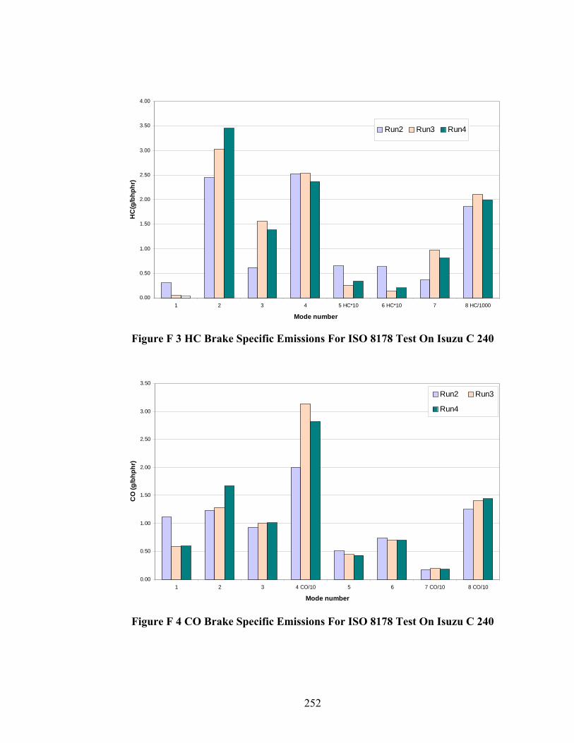
I I

1 li!!II I

-1,,111111,, ,,11111,

~

-

-

--- - -

-- ,_ -

- - -- ,_ ,_ - -

n_ jl =II i -

~

111111

--- --- - -- ---- ,- ,- - -

-~- [I -

3.50

0.00

0.50

1.00

1.50

2.00

2.50

3.00

3.50

4.00

HC

(g/b

hphr

) Run2 Run3 Run4

1 2 3 4 5 HC*10 6 HC*10 7 8 HC/1000

Mode number

Figure F 3 HC Brake Specific Emissions For ISO 8178 Test On Isuzu C 240

CO

(g/b

hphr

)

3.00

2.50

2.00

1.50

1.00

0.50

0.00

Run2 Run3

Run4

1 2 3 4 CO/10 5 6 7 CO/10 8 CO/10

Mode number

Figure F 4 CO Brake Specific Emissions For ISO 8178 Test On Isuzu C 240

252

llii1

I

-~ ---

4500.00

4000.00

3500.00

3000.00

CO

2 (g

/bhp

hr)

2500.00

2000.00

1500.00

1000.00

500.00

0.00

Figure F 5 CO2 Brake Specific Emissions For ISO 8178 Test On Isuzu C 240

Run1 Run2 Run3 Run4

1 2 3 4 5 6 7 8

Mode number

0.00

2.00

4.00

6.00

8.00

10.00

12.00

14.00

16.00

18.00

NO

x (g

/bhp

hr)

Run1 Run2 Run3

1 2 3 4 5 6 7 8 NOx/10

Mode number

Figure F 6 NOx Brake Specific Emissions For ISO 8178 Test On DDC Series 60

253

I~ [3 I -

-

H HI!'

-

-

Ml 1111 Im 1111 I I I I I I I I

[~ I

-

-_ ,..,,,,. ~

>--

-- ----- - -~ - ~ - ~ -

>-- - - --- -~ ~ - ~ - ~ ~

rlJ7

0.000

0.050

0.100

0.150

0.200

0.250

0.300

0.350

0.400

0.450

PM (g

/bhp

hr)

Run1 Run2 Run3

1 2 3 4 5 6 7 8 PM/100

Mode number

Figure F 7 PM Brake Specific Emissions For ISO 8178 Test On DDC Series 60

0.14

HC

(g/b

hphr

)

0.12

0.10

0.08

0.06

0.04

0.02

0.00

Run1 Run2 Run3

1 2 3 4 HC/10 5 6 7 8 HC/1000

Mode number

Figure F 8 HC Brake Specific Emissions For ISO 8178 Test On DDC Series 60

254

0.00

0.50

1.00

1.50

2.00

2.50

3.00

3.50

4.00

4.50

5.00

CO

(g/b

hphr

) Run1 Run2 Run3

lo i:::J ~ - I

- -- -

H IIII•

-

- -- - - -

rm,,-

- - -

- - -- -- J17- - - rn- ~

I I I I Im -

I I I I

I

I

-

---- --

-

- - ---- -- - - - - - ~ - -

- - - - - - ~ - -

1 2 3 4 CO/10 5 6 7 8 CO/100

Mode number

Figure F 9 CO Brake Specific Emissions For ISO 8178 Test On DDC Series 60

1200

CO

2 (g

/bhp

hr)

1000

800

600

400

200

0

Run1 Run2 Run3

1 2 3 4 5 6 7 8 CO2/10

Mode number

Figure F 10 CO2 Brake Specific Emissions For ISO 8178 Test On DDC Series 60

255

I I I I 11 I I

Appendix G

. Com

parison of Mass E

missions R

ates of NO

x and CO

2 Betw

een ME

MS and C

VS

Laboratory for ISO

8178 8-Mode T

ests on DD

C Series 60 and on Isuzu C

240 Engines

0.07

-0.01

Time (sec)

Appendix G

1 Figure G 1 C

omparison of M

EM

S Vs L

ab For ISO 8178 8 M

ode Test O

n Isuzu C

240 Run 1

-2 0 2 4 6 8 10 0 500

1000 1500

2000 2500

3000

CO2 (g/s)

0

ME

MS

CO

2 Trace Lab C

O2 Trace

Lab NO

X Trace

ME

MS

NO

x Trace

0.06

0.05

0.04

0.03

0.02

0.01

NOx (g/sec)

-2 0 2 4 6 8 10 0 500

1000 1500

2000 2500

CO2 (g/sec)

-0.01

0 0.01

0.02

0.03

0.04

0.05

NOx (g/s)

lab CO

2 Trace M

EMS

CO

2 Trace Lab N

Ox Trace

MEM

S N

Ox Trace

Time (sec)

Figure G 2 C

omparison of M

EM

S Vs L

ab For ISO 8178 8 M

ode Test O

n Isuzu C 240 R

un 2

256

... 1 II ---~-. - ...,... . -

'---

--~ - ... , --

II ~

r-1,. . I ---..... ~· B \¼l\v -I"" ,._

-- ~

t,,,/>AJ~N•• I. . . -· I -· I/ ,,. -.. ~ \.;..,.,,

ll'I""

... _ . - ~_z_;rt~"!;-... _ _,, .. ,

T .

. ~

10 0.07

CO

2 (g/

bhph

r)

9

8

7

9

8

7

6

5

4

3

2

1

0 0 500 1000 1500 2000 2500 3000

Time (sec)

MEMS CO2 Trace Lab CO2 Trace MEMS NOx Trace Lab NOx Trace

0.06

0.05

0.04

0.03

0.02

0.01

NO

x (g/

bhph

r)

-1 0

Figure G 3 Comparison of MEMS Vs Lab For ISO 8178 8 Mode Test On Isuzu C 240 Run 3

0.0710

0 500 1000 1500 2000 2500 3000

Time (sec)


-1 0

0.06

0.05

0.04

0.03

0.02

0.01

CO

2 (g/

bhph

r)

6

5

4

3

2

1

0

NO

x (g/

bhph

r)

Figure G 4 Comparison of MEMS Vs Lab For ISO 8178 8 Mode Test On Isuzu C 240 Run 4

257

' ~., --- - -

-

'

-~

- .. ...,._,,,,,_ . ..,.

t~-_j .. , , --

~ ~-

,_,_.

I -r- • • •

0

60 0.9

0 500 1000 1500 2000 2500 3000

Time (s)

0

MEMS CO2 Trace Lab CO2 Trace Lab NOx Trace MEMS NOx Trace

0.8

0.7

0.6

0.5

0.4

0.3

0.2

0.1

CO

2 (g/

bhph

r)

50

40

30

20

10

0

NO

x (g/

bhph

r)

-10 -0.1

Figure G 5 Comparison of MEMS Vs Lab For ISO 8178 8 Mode Test On DDC Series 60 Run

60 0.9

30

0 400 800 1200 1600 2000 2400 2800 3200 3600 400

Time (secs)


0.4

20 0.3

0.210

0.1

0

0.8 50

0.7

0.6

0.5

40

CO

2 (g/

bhph

r)

NO

x (g/

bhph

r)

0

-10 -0.1

Figure G 6 Comparison of MEMS Vs Lab For ISO 8178 8 Mode Test On DDC Series 60 Run 2

258

ll I -.,

-,_ I•

.,

~ l - -..._.- .. - -- .. - -..

L_ ~- - - -- JI

0.000

0.100

0.200

0.300

0.400

0.500

0.600

0.700

0.800

0.900

1.000

NO

x (g/

bhph

r)

-10.000

0.000

10.000

20.000

30.000

40.000

50.000

CO

2 (g/

bhph

r)

MEMS NOx Trace Lab NOx Trace MEMS CO2 Trace Lab CO2 Trace

0.00 500.00 1000.00 1500.00 2000.00 2500.00 3000.00

Time (sec)

Figure G 7 Comparison of MEMS Vs Lab For ISO 8178 8 Mode Test On DDC Series 60 Run 3

259

Appendix H. ISO 8178 Test Detail Results on Isuzu C240 and DDC Series 60.

Table H 1 ISO 8178 TEST RESULTS ON ISUZU C 240 RUN 1

ISO 8178 TEST MODE




Percent Difference


R100 681.96 3.37 616.17 3.44 10.68 -2.21 R75 699.07 3.85 643.98 4.10 8.55 -6.12 R50 810.18 4.04 751.45 4.42 7.81 -8.42 R10 4288.36 13.83 4143.65 16.20 3.49 -14.60 I100 661.89 2.19 586.21 2.25 12.91 -3.02 I75 667.09 3.61 587.09 3.51 13.63 2.69 I50 722.46 5.10 583.98 3.92 23.71 30.00




ISO 8178 TEST MODE

Average HC, CO and PM Mass Emissions in g/bhp-hr From Lab for ISO 8178 test on Isuzu C 240. Run1

HC CO PM R100 0.31 4.78 0.0 R75 2.05 5.37 0.0 R50 0.42 4.29 0.0 R10 3.69 104.76 0.0 I100 0.11 2.32 0.0 I75 0.15 3.59 0.0 I50 1.99 14.38 0.0

IDLE 1964.55 12.62 0.0 Weighted average

emissions for the cycle 295.69 16.56 0.0

260


ISO 8178 TEST MODE




Percent Difference


R100 680.65 4.30 612.33 4.27 11.16 0.71 R75 693.18 4.92 640.27 5.03 8.26 -2.20 R50 779.41 5.30 738.64 5.53 5.52 -4.15 R10 3806.21 14.99 3552.29 17.39 7.15 -13.81 I100 669.97 2.99 572.23 2.66 17.08 12.37 I75 644.06 4.72 575.00 4.33 12.01 9.04 I50 647.91 5.89 606.35 5.67 6.86 3.80




ISO 8178 TEST MODE


HC CO PM R100 0.30 1.12 0.147 R75 2.45 1.24 0.175 R50 0.62 0.93 0.149 R10 2.53 20.06 0.909 I100 0.06 0.51 0.148 I75 0.06 0.74 0.079 I50 0.36 1.80 0.088




ISO 8178 TEST MODE




Percent Difference


R100 624.21 4.11 641.71 3.78 -2.73 8.82 R75 650.23 5.47 661.36 5.19 -1.68 5.56 R50 750.68 6.39 756.60 5.67 -0.78 12.65 R10 4118.55 20.93 4018.61 17.61 2.49 18.86 I100 770.20 3.69 643.67 2.74 19.66 34.60 I75 644.04 4.71 608.91 4.11 5.77 14.53 I50 695.20 5.20 705.76 4.86 -1.50 6.93

IDLE 2124.81 14.05 2034.77 15.49 4.42 -9.30 Weighted average


261


ISO 8178 TEST MODE


HC CO PM R100 0.31 4.78 0.176 R75 2.05 5.37 0.392 R50 0.42 4.29 0.211 R10 3.69 104.76 1.655 I100 0.11 2.32 0.190 I75 0.15 3.59 0.096 I50 1.99 14.38 0.171




ISO 8178 TEST MODE




Percent Difference


R100 622.95 4.12 643.82 3.82 -3.24 7.95 R75 639.97 5.33 657.11 5.06 -2.61 5.14 R50 758.45 6.18 761.09 5.48 -0.35 12.72 R10 3763.56 18.63 3661.21 15.76 2.80 18.23 I100 744.46 3.63 627.42 2.74 18.66 32.35 I75 639.32 4.50 606.00 3.79 5.50 18.81 I50 616.35 5.05 626.97 4.82 -1.69 4.74



262


ISO 8178 TEST MODE

Average HC, CO and PM Mass Emissions in g/bhp-hr From Lab for

ISO 8178 test on DDC Series 60. Run4 HC CO PM

R100 0.31 4.81 0.16 R75 2.03 5.32 0.37 R50 0.42 4.31 0.24 R10 3.32 94.34 1.69 I100 0.11 2.26 0.20 I75 0.15 3.57 0.09 I50 1.77 12.85 0.16



Table H 9 ISO 8178 TEST RESULTS ON DDC SERIES 60 RUN 1

ISO 8178 TEST MODE





Percent Difference


R100 488.93 8.05 500.95 8.26 -2.40 -2.53 R75 459.88 8.71 470.62 8.83 -2.28 -1.32 R50 467.68 10.24 485.49 10.74 -3.67 -4.68 R10 768.34 13.13 773.39 13.87 -0.65 -5.35 I100 498.31 7.18 489.62 7.21 1.78 -0.39 I75 484.85 7.95 471.44 8.14 2.84 -2.34 I50 481.54 9.83 469.83 10.43 2.49 -5.76



263


ISO 8178 TEST MODE



R100 0.05 0.48 0.048 R75 0.06 0.33 0.047 R50 0.08 0.49 0.057 R10 0.44 1.34 0.337 I100 0.12 0.86 0.089 I75 0.05 4.43 0.062 I50 0.05 2.94 0.029




ISO 8178 TEST MODE





Percent Difference


R100 473.31 8.11 493.37 8.11 -4.07 0.00 R75 449.87 8.74 468.48 8.83 -3.97 -0.97 R50 447.99 10.15 482.77 10.84 -7.21 -6.33 R10 702.79 12.92 778.24 14.88 -9.70 -13.18 I100 471.89 6.78 487.64 7.01 -3.23 -3.25 I75 461.34 7.46 471.15 7.77 -2.08 -4.00 I50 467.06 9.46 472.92 9.97 -1.24 -5.13


emissions for the cycle 1593.98 29.90 1603.59 28.30 0.60 -5.65

264


ISO 8178 TEST MODE



R100 0.05 0.47 0.049 R75 0.05 0.32 0.040 R50 0.08 0.32 0.049 R10 0.88 6.71 0.353 I100 0.04 3.32 0.084 I75 0.04 1.84 0.062 I50 0.03 0.54 0.029




ISO 8178 TEST MODE





Percent Difference


R100 428.60 7.00 462.84 8.19 -7.40 -14.61 R75 418.53 6.81 466.00 8.59 -10.19 -20.73 R50 440.85 7.58 482.56 10.29 -8.64 -26.33 R10 769.27 15.71 825.36 16.39 -6.80 -4.15 I100 428.50 5.72 451.28 6.23 -5.05 -8.05 I75 463.08 6.94 469.18 7.53 -1.30 -7.93 I50 505.43 9.36 473.31 9.66 6.79 -3.12


emissions for the cycle 1556.14 25.50 1410.86 29.04 -10.30 12.18

265


ISO 8178 TEST MODE



R100 0.04 0.56 0.048 R75 0.04 0.34 0.040 R50 0.05 0.28 0.049 R10 0.68 4.74 0.405 I100 0.02 3.21 0.089 I75 0.03 2.32 0.065 I50 0.02 0.62 0.031



266

Cc,,ec.~I -, Jq ..

~r<\(510~

------ Barometric Pressure Pb &q, ( b '. I- a Calibration Device# Control Box Number Meter Serial Number ------ Ambient Temperature ______ Calibration Device y

111\l'.l

Orifice sqm

Gas Volume of Calibration

·rn Sc f

Temperature Measurements Calibration I Dry Gas Meter

• R. Meler Outlet

Tc1o s-1

Average Meter

~. '3 (:, ! ,G .. I v,/S: I r,-, .. , · ! J <.J•·r: i 5)] •,)1 '-'O i n1u i ~ I ~97"> 1 .,._-(\.,i i l ....... Y _,... C; •~1q ~e-v l\Y ., ,,,-,4

AH@ -l ·~i, ?-· ·31H -- ,._,

2 Vw Pb (Td + 460)

0.0317 ,\II [ (T.+460)0] V, ~ ,+ : 6 ) (T.+460) Pb (Td + 460) Vw

':,jm~TD") -;:. It· by X f X \Jm. ><. ( Pb~ + L)o/i3-6)

- 1--,

Appendix I.

Calibration Sheet for the D

ry Gas M

eter

Figure I1: Calibration of the dry gas m

eter. The m

eter was calibrated using an 8

cfm L

aminar Flow

Elem

ent from M

eriam Instrum

ents ®.

267

Appendix J. Procedure to Leak Check the Control Console of the Method 5 Sampling System

The following is a positive pressure leak check procedure that will check the metering system from the sample inlet quick connect to the orifice outlet including the inclined manometer.

The orifice meter line downstream of the orifice is disconnected and the pressure tap is plugged. The negative side of the inclined manometer is vented. A one-hole rubber stopper with a tube through its hole is placed into the exit of the orifice.

With the positive side of the manometer enabled, coarse and fine valves open completely, a vacuum pump is connected to the system through the tubing into the one hole rubber stopper. Air is blown into the system until a pressure of 6 inches H2O is seen in the manometer. The pump is then shut to form a closed loop to maintain pressure. The reading on the manometer is noted for a period of one minute. If there is any noticeable movement in the fluid level of the monometer, then Snoop® (bubbling type, soapy water) is used to detect the leak.

268

Report: 2004-04-29 Development of a Test Method to Measure ...

Documents

Transcript of Report: 2004-04-29 Development of a Test Method to Measure ...